CHAPTER 2

SCATTER PLOTS, CORRELATION, LINEAR REGRESSION, INFERENCES FOR REGRESSION

By: Tasha Carr, Lyndsay Gentile, Darya Rosikhina, Stacey Zarko

SCATTER PLOTS Shows the relationship between two

quantitative variables measured on the same individuals

Look at:Direction- positive, negative, noneForm-straight, linear, curvedStrength- little scatter means little association

great scatter means great association

Outliers- make sure there are no major outliers

Measures the direction and strength of the linear relationship

Usually written as rr is the correlation coefficientNot resistant

CORRELATION

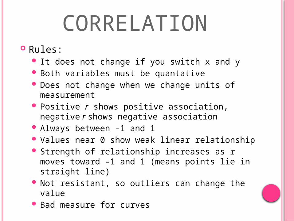
Rules: It does not change if you switch x and y Both variables must be quantative Does not change when we change units of

measurement Positive r shows positive association, negative r

shows negative association Always between -1 and 1 Values near 0 show weak linear relationship Strength of relationship increases as r moves

toward -1 and 1 (means points lie in straight line) Not resistant, so outliers can change the value Bad measure for curves

CORRELATION

Makes the sum of the squares of the vertical distances of the data points from the line as small as possible (not resistant)

Ŷ = b0 + b1 x

b1 x = slope b1 = (sy / sx )(r) Amount by which y changes when x increases by

one unit

b0 = y-intercept Value of y when x=0 b0 = (y-bar) - b1 x

Extrapolation- making predictions outside of the given data ; inaccurate

LEAST-SQUARES REGRESSION

A Regression Line is a straight line that describes how a response variable as an explanatory variable x changes

Based on correlation Used to predict the value of y for a

given value of x R2 = Coefficient of Determination

In the model, R2 of the variability in the y-

variable is accounted for by variation in the x-

variable.

LEAST-SQUARES REGRESSION

Minimized by the LSRL Difference between actual and

predicted dataObserved – ExpectedActual – Guesse = Y – ŶPositive residuals – underestimatesNegative residuals – overestimates

RESIDUALS

A scatter plot of the regression residuals against the explanatory variable or predicted values

Shows if linear model is appropriate If there is no apparent shape or pattern and

residuals are randomly scattered, linear model is a good fit

If there is a curve or horn shape, or big change in scatter, linear model is not a good fit

RESIDUAL PLOT

Variable that has an important effect on the relationship among the variables in a study but is not included among the variables studied Make a correlation or regression misleading

An outlier- point that lies outside the overall pattern of the other observations

Influential point- removing it would change the outcome (outliers in the x- direction)

LURKING VARIABLES

An association between an explanatory and response variable does not show a causation, or cause and effect relationship, even if there is a high correlation

Correlation based on averages is higher than data from individuals

CAUSATION

Used to test if there is an association between two quantitative variables based on the population

To test for an association we check β1 If no association exists this

should be zero

INFERENCE FOR REGRESSION

Hypothesis: H0 : β1 = 0. There is no association HA : β1 ≠ 0. There is an association.

Conditions: Straight Enough: Check for no curves in scatter

plot. Independence: Data is assumed independent. Equal Variance: Check residual plot for changes

in spread Nearly Normal: Create histogram or Normal

Probability plot of the residuals. All conditions have been met to use a student’s

t-model for a test on the slope of a regression model.

INFERENCE FOR REGRESSION

Mechanics Df = n – 2 t= (b1 – 0)/(SE(b1 ) P-value = 2P(tn-2 > or < t)

b0

b1

INFERENCE FOR REGRESSION

Model of House Prices Multiple Regression

Response attribute (numeric): Price

R-Squared: 0.0284526Adjusted R-Squared: 0.0137322Standard Deviation of the Error: 400.242

Std t P

Predictor Coefficient Error Statistic Value R2

Constant 1244.2712 75.4607 16.489 -0.0000

Age -5.3659 3.8596 -1.390 0.1691 0.0285

Regression Equation: Price = Age

SE (b1 )t= (b1 – 0)/(SE(b1 )

P-value

Conclusion If the p-value is less than alpha, reject the

null hypothesisIf we reject H0, there is evidence of an association

If the p-value is greater than alpha, we fail to reject the null hypothesisIf we fail to reject the H0 , there is not enough evidence of an association

INFERENCE FOR REGRESSION