Embed Size (px)
Citation preview
Chapter 2
Linear Algebra
Linear algebra is about linear systems of equations and their solutions. As asimple example, consider the following system of two linear equations withtwo unknowns:
2x1 ! x2 = 1
x1 + x2 = 5.
There is a unique solution, given by x1 = 2 and x2 = 3. One way to seethis is by drawing a graph, as shown in Figure 2.1. One line in the figurerepresents the set of pairs (x1, x2) for which 2x1 ! x2 = 1, while the otherrepresents the set of pairs for which x1 +x2 = 5. The two lines intersect onlyat (2, 3), so this is the only point that satisfies both equations.
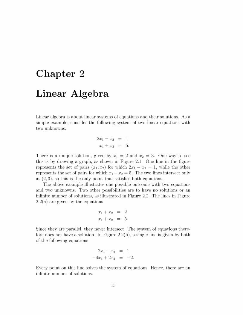
The above example illustrates one possible outcome with two equationsand two unknowns. Two other possibilities are to have no solutions or aninfinite number of solutions, as illustrated in Figure 2.2. The lines in Figure2.2(a) are given by the equations
x1 + x2 = 2
x1 + x2 = 5.
Since they are parallel, they never intersect. The system of equations there-fore does not have a solution. In Figure 2.2(b), a single line is given by bothof the following equations
2x1 ! x2 = 1
!4x1 + 2x2 = !2.
Every point on this line solves the system of equations. Hence, there are aninfinite number of solutions.
15

16
(2, 3)
(-0.5, 0)
(0, -1)
(5, 0)
(0, 5)
x1
x2
Figure 2.1: A system of two linear equations with two unknowns, with a uniquesolution.
There is no way to draw two straight lines on a plane so that they onlyintersect twice. In fact, there are only three possibilities for two lines on aplane: they never intersect, intersect once, or intersect an infinite number oftimes. Hence, a system of two equations with two unknowns can have eitherno solution, a unique solution, or an infinite number of solutions.
Linear algebra is about such systems of linear equations, but with manymore equations and unknowns. Many practical problems benefit from in-sights o!ered by linear algebra. Later in this chapter, as an example of howlinear algebra arises in real problems, we explore the analysis of contingentclaims. Our primary motivation for studying linear algebra, however, is todevelop a foundation for linear programming, which is the main topic of thisbook. Our coverage of linear algebra in this chapter is neither self-containednor comprehensive. A couple of results are stated without any form of proof.The concepts presented are chosen based on their relevance to the rest of thebook.
c"Benjamin Van Roy and Kahn Mason 17
(5, 0)
(0, 5)
x1
x2
(2, 0)
(0, 2)
(-0.5, 0)
(0, -1)
x1
x2
(a) (b)
Figure 2.2: (a) A case with no solution. (b) A case with an infinite number ofsolutions.
2.1 Matrices
We assume that the reader is familiar with matrices and their arithmeticoperations. This section provides a brief review and also serves to definenotation that we will be using in the rest of the book. We will denote the setof matrices of real numbers with M rows and N columns by #M!N . Given amatrix A $ #M!N , we will use the notation Aij to refer to the entry in theith row and jth column, so that
A =
!
""""#
A11 A12 · · · A1N
A21 A22 · · · A2N...
... · · · ...AM1 AM2 · · · AMN
$
%%%%&.
2.1.1 Vectors
A column vector is a matrix that has only one column, and a row vector isa matrix that only has one row. A matrix with one row and one columnis a number. For shorthand, the set of column vectors with M componentswill be written as #M . We will primarily employ column vectors, and assuch, when we refer to a vector without specifying that it is a row vector, it

18
should be taken to be a column vector. Given a vector x $ #M , we denotethe ith component by xi. We will use the notation Ai" for the column vectorconsisting of entries of the ith row. Similarly, A"j will be the column vectormade up of the jth column of the matrix.
2.1.2 Addition
Two matrices can be added if they have the same number of rows and thesame number of columns. Given A, B $ #M!N , entries of the matrix sumA + B are given by the sums of entries (A + B)ij = Aij + Bij. For example,
'1 23 4
(
+
'5 67 8
(
=
'6 810 12
(
.
Multiplying a matrix by a scalar ! $ # involves scaling each entry by !.In particular, given a scalar ! $ # and a matrix A $ #M!N , we have(!A)ij = (A!)ij = !Aij. As an example,
2
'1 23 4
(
=
'2 46 8
(
.
Note that matrix addition is commutative (so, A+B = B+A) and associative((A + B) + C = A + (B + C) =: A + B + C) just like normal addition. Thismeans we can manipulate addition-only equations with matrices in the sameways we can manipulate normal addition-only equations. We denote by 0any matrix for which all of the elements are 0.
2.1.3 Transposition
We denote the transpose of a matrix A by AT . If A is an element of #M!N ,AT is in #N!M , and each entry is given by (AT )ij = Aji. For example,
!
"#1 23 45 6
$
%&
T
=
'1 3 52 4 6
(
.
Clearly, transposition of a transpose gives the original matrix: ((AT )T )ij =(AT )ji = Aij. Note that the transpose of a column vector is a row vectorand vice-versa. More generally, the columns of a matrix become rows of itstranspose and its rows become columns of the transpose. In other words,(AT )i" = A"i and (AT )"j = Aj".
c"Benjamin Van Roy and Kahn Mason 19
2.1.4 Multiplication
A row vector and a column vector can be multiplied if each has the samenumber of components. If x, y $ #N , then the product xT y of the row vectorxT and column vector y is a scalar, given by xT y =
)Ni=1 xiyi. For example,
*1 2 3
+!
"#456
$
%& = 1% 4 + 2% 5 + 3% 6 = 32.
Note that xT x =)N
i=1 x2i is positive unless x = 0 in which case it is 0. Its
square root (xT x)1/2 is called the norm of x. In three-dimensional space,the norm of a vector is just its Euclidean length. For example, the norm of[4 5 6]T is
&77.
More generally, two matrices A and B can be multiplied if B has exactlyas many rows as A has columns. The product is a matrix C = AB that hasas many rows as A and columns as B. If A $ #M!N and B $ #N!K then theproduct is a matrix C $ #M!K , whose (i, j)th entry is given by the productof Ai", the ith row of A and B"j, the jth column of B; in other words,
Cij = (Ai")T B"j =
N,
k=1
AikBkj.
For example,'
1 2 34 5 6
( !
"#456
$
%& =
'3277
(
Like scalar multiplication, matrix multiplication is associative (i.e., (AB)C =A(BC)) and distributive (i.e., A(B + C) = AB + AC and (A + B)C =AC + BC), but unlike scalar multiplication, it is not commutative (i.e., ABis generally not equal to BA). The first two facts mean that much of ourintuition about the multiplication of numbers is still valid when applied tomatrices. The last fact means that not all of it is – the order of multiplicationis important. For example,
*1 2
+ '34
(
= 11, but
'34
( *1 2
+=
'3 64 8
(
.
A matrix is square if the number of rows equals the number of columns.The identity matrix is a square matrix with diagonal entries equal to 1 andall other entries equal to 0. We denote this matrix by I (for any number ofrows/columns). Note that for any matrix A, IA = A and AI = A, given
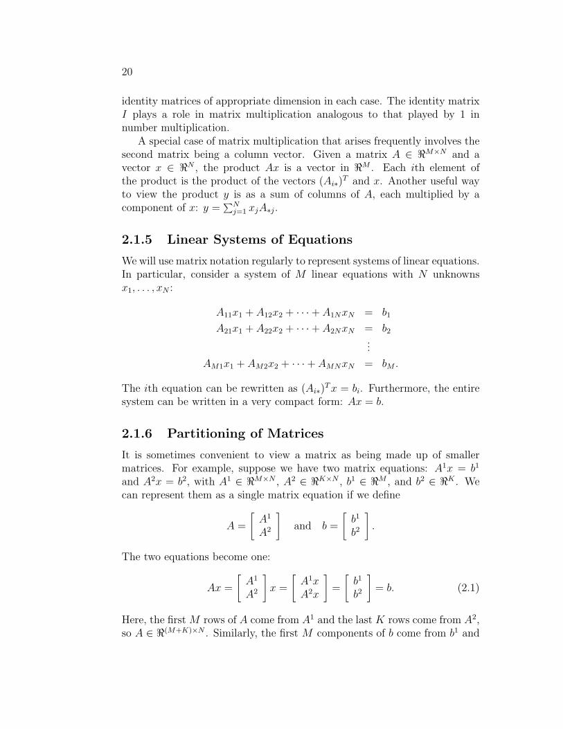
20
identity matrices of appropriate dimension in each case. The identity matrixI plays a role in matrix multiplication analogous to that played by 1 innumber multiplication.
A special case of matrix multiplication that arises frequently involves thesecond matrix being a column vector. Given a matrix A $ #M!N and avector x $ #N , the product Ax is a vector in #M . Each ith element ofthe product is the product of the vectors (Ai")T and x. Another useful wayto view the product y is as a sum of columns of A, each multiplied by acomponent of x: y =
)Nj=1 xjA"j.
2.1.5 Linear Systems of Equations
We will use matrix notation regularly to represent systems of linear equations.In particular, consider a system of M linear equations with N unknownsx1, . . . , xN :
A11x1 + A12x2 + · · · + A1NxN = b1
A21x1 + A22x2 + · · · + A2NxN = b2
...
AM1x1 + AM2x2 + · · · + AMNxN = bM .
The ith equation can be rewritten as (Ai")T x = bi. Furthermore, the entiresystem can be written in a very compact form: Ax = b.
2.1.6 Partitioning of Matrices
It is sometimes convenient to view a matrix as being made up of smallermatrices. For example, suppose we have two matrix equations: A1x = b1
and A2x = b2, with A1 $ #M!N , A2 $ #K!N , b1 $ #M , and b2 $ #K . Wecan represent them as a single matrix equation if we define
A =
'A1
A2
(
and b =
'b1
b2
(
.
The two equations become one:
Ax =
'A1
A2
(
x =
'A1xA2x
(
=
'b1
b2
(
= b. (2.1)
Here, the first M rows of A come from A1 and the last K rows come from A2,so A $ #(M+K)!N . Similarly, the first M components of b come from b1 and
c"Benjamin Van Roy and Kahn Mason 21
the last K components come from b2, and b $ #M+K . The representation ofa matrix in terms of smaller matrices is called a partition.
We can also partition a matrix by concatenating two matrices with thesame number of rows. Suppose we had two linear equations: Ax1 = b1 andAx2 = b2. Note that the vectors x1 and x2 can take on di!erent values,while the two equations share a common matrix A. We can concatenate x1
and x2 because they have the same number of components (they must tobe multiplied by A). Similarly, we can concatenate b1 and b2. If we writeX = [x1 x2] and B = [b1 b2] then we again have AX = B. Note that now Xand B are not vectors; they each have 2 columns. Writing out the matricesin terms of partitions, we have
A*x1 x2
+=
*b1 b2
+. (2.2)
Given the same equations, we could alternatively combine them to forma single equation
'A 00 A
( 'x1
x2
(
=
'Ax1 + 0x2
0x1 + Ax2
(
=
'Ax1
Ax2
(
=
'b1
b2
(
,
where the 0 matrix has as many rows and columns as A.Note that, for any partition, the numbers of rows and columns of com-
ponent matrices must be compatible. For example, in Equation (2.1), thematrices A1 and A2 had to have the same number of columns in order forthe definition of A to make sense. Similarly, in Equation (2.2), x1 and x2
must have the same number of components, as do b1 and b2. More generally,we can partition a matrix by separating rows, columns, or both. All that isrequired is that each component matrix has the same number of columns asany other component matrix it adjoins vertically, and the same number ofrows as any other component matrix it adjoins horizontally.
2.2 Vector Spaces
The study of vector spaces comprises a wealth of ideas. There are a numberof complexities that arise when one deals with infinite-dimensional vectorspaces, and we will not address them. Any vector space we refer to in thisbook is implicitly assumed to be finite-dimensional.
Given a collection of vectors a1, . . . , aN $ #M , the term linear combina-tion refers to a sum of the form
N,
j=1
xjaj,
22
for some real-valued coe"cients x1, . . . , xN . A finite-dimensional vector spaceis the set S of linear combinations of a prescribed collection of vectors. Inparticular, a collection of vectors a1, . . . , aN $ #M generates a vector space
S =
-.
/
N,
j=1
xjaj
000 x $ #M
12
3 .
This vector space is referred to as the span of the vectors a1, . . . , aN used togenerate it. As a convention, we will take the span of an empty set of vectorsto be the 0-vector; i.e., the vector with all components equal to 0.
If a vector x is in the span of a1, . . . , aN , we say x is linearly dependent ona1, . . . , aN . On the other hand, if x is not in the span of a1, . . . , aN , we sayx is linearly independent of a1, . . . , aN . A collection of vectors, a1, . . . , aN iscalled linearly independent if none of the vectors in the collection is linearlydependent on the others. Note that this excludes the 0-vector from any setof linearly independent vectors. The following lemma provides an equivalentdefinition of linear independence.
Lemma 2.2.1. A collection of vectors a1, . . . , aN is linearly independent if)Nj=1 !jaj = 0 implies that !1 = !2 = · · · = !N = 0.
One example of a vector space is the space #M itself. This vector spaceis generated by a collection of M vectors e1, . . . , eM $ #M . Each ei denotesthe M -dimensional vector with all components equal to 0, except for the ithcomponent, which is equal to 1. Clearly, any element of #M is in the spanof e1, . . . , eM . In particular, for any y $ #M ,
y =M,
i=1
yiei,
so it is a linear combination of e1, . . . , eM .More interesting examples of vector spaces involve nontrivial subsets of
#M . Consider the case of M = 2. Figure 2.3 illustrates the vector spacegenerated by the vector a1 = [1 2]T . Suppose we are given another vectora2. If a2 is a multiple of a1 (i.e., a2 = !a1 for number !), the vector spacespanned by the two vectors is no di!erent from that spanned by a1 alone. Ifa2 is not a multiple of a1 then any vector in y $ #2 can be written as a linearcombination
y = x1a1 + x2a
2,
and therefore, the two vectors span #2. In this case, incorporating a thirdvector a3 cannot make any di!erence to the span, since the first two vectorsalready span the entire space.

c"Benjamin Van Roy and Kahn Mason 23
a(1)
Figure 2.3: The vector space spanned by a1 = [1 2]T .
The range of possibilities increases when M = 3. As illustrated in Figure2.4(a), a single vector spans a line. If a second vector is not a multiple of thefirst, the two span a plane, as shown in 2.4(b). If a third vector is a linearcombination of the first two, it does not increase the span. Otherwise, thethree vectors together span all of #3.
Sometimes one vector space is a subset of another. When this is the case,the former is said to be a subspace of the latter. For example, the vectorspace of Figure 2.4(a) is a subspace of the one in Figure 2.4(b). Both ofthese vector spaces are subspaces of the vector space #3. Any vector spaceis a subset and therefore a subspace of itself.
2.2.1 Bases and Dimension
For any given vector space S, there are many collections of vectors that spanS. Of particular importance are those with the special property that theyare also linearly independent collections. Such a collection is called a basis.
To find a basis for a space S, one can take any spanning set, and repeat-edly remove vectors that are linear combinations of the remaining vectors.

24
a(1) a(1) a (2)
(a) (b)
Figure 2.4: (a) The vector space spanned by a single vector a1 $ #3. (b) Thevector space spanned by a1 and a2 $ #3 where a2 is not a multiple of a1.
At each stage the set of vectors remaining will span S, and the process willconclude when the set of vectors remaining is linearly independent. That is,with a basis.
Starting with di!erent spanning sets will result in di!erent bases. Theyall however, have the following property, which is important enough to stateas a theorem.
Theorem 2.2.1. Any two bases of a vector space S have the same numberof vectors.
We prove this theorem after we establish the following helpful lemma:
Lemma 2.2.2. If A = {a1, a2, . . . , aN} is a basis for S, and if b = !1a1 +!2a2 + . . . + !NaN with !1 '= 0, then {b, a2, . . . , aN} is a basis for S.
Proof of lemma: We need to show that {b, a2, . . . , aN} is linearly indepen-dent and spans S. Note that a1 = 1
!1b! !2
!1a2 ! . . . + !NaN
!1.
To show linear independence, note that the ai’s are linearly independent,so the only possibility for linear dependence is if b is a linear combinationof a2, . . . , aN . But a1 is a linear combination of b, a2, . . . , aN , so this wouldmake a1 a linear combination of a2, . . . , aN , which contradicts the fact that

c"Benjamin Van Roy and Kahn Mason 25
a1, . . . , aN are linearly independent. Thus b must be linearly independent ofa2, . . . , aN , and so the set is linearly independent.
To show that the set spans S, we just need to show that it spans a basisof S. It obviously spans a2, . . . , an, and because a1 is a linear combination ofb, a2, . . . , an we know the set spans S.
Proof of theorem: Suppose A = {a1, a2, . . . , aN} and B = {b1, b2, . . . , bM}are two bases for S with N > M . Because A is a basis, we know thatb1 = !1a1 + !2a2 + . . . + !NaN for some !1, !2, . . . ,!N where not all the !i’sare equal to 0. Assume without loss of generality that !1 '= 0. Then, byLemma 2.2.2, A1 = {b1, a2, . . . , aN} is a basis for S.
Now, because A1 is a basis for S, we know that b2 = "1b1 + !2a2 +. . .+!NaN for some "1, !2, . . . ,!N where we know that not all of !2, . . . ,!N
are equal to 0 (otherwise b2 would be linearly dependent on b1, and so Bwould not be a basis). Note the !i’s here are not the same as those for b1
in terms of a1, a2, . . . , aN . Assume that !2 '= 0. The lemma now says thatA2 = {b1, b2, a3 . . . , aN} is a basis for S.
We continue in this manner, substituting bi into Ai#1 and using the lemmato show that Ai is a basis for S, until we arrive at AM = {b1, . . . , bM , aM+1, . . . , aN}this cannot be a basis for S because aM+1 is a linear combination of {b1, . . . , bM}.This contradiction means that N cannot be greater than M . Thus any twobases must have the same number of vectors.
Let us motivate Theorem 2.2.1 with an example. Consider a plane inthree dimensions that cuts through the origin. It is easy to see that sucha plane is spanned by any two vectors that it contains, so long as they arelinearly independent. This means that any additional vectors cannot belinearly independent. Since the first two were arbitrary linearly independentvectors, this indicates that any basis of the plane has two vectors.
Because the size of a basis depends only on S and not on the choice ofbasis, it is a fundamental property of S. It is called the dimension of S. Thisdefinition corresponds perfectly with the standard use of the word dimension.For example, dim(#M) = M because e1, . . . , eM is a basis for #M .
Theorem 2.2.1 states that any basis of a vector space S has dim(S) vec-tors. However, one might ask whether any collection of dim(S) linearlyindependent vectors in S spans the vector space. The answer is provided bythe following theorem:
Theorem 2.2.2. For any vector space S ( #M , each linearly independentcollection of vectors a1, . . . , adim(S) $ S is a basis of S.
Proof: Let b1, . . . , bK be a collection of vectors that span S. Certainly the set

26
{a1, . . . , adim(S), b1, . . . , bK} spans S. Consider repeatedly removing vectors bi
that are linearly dependent on remaining vectors in the set. This will leave uswith a linearly independent collection of vectors comprised of a1, . . . , adim(S)
plus any remaining bi’s. This set of vectors still spans S, and therefore, theyform a basis of S. From Theorem 2.2.1 this means it has dim(S) vectors.It follows that the remaining collection of vectors cannot include any bi’s.Hence, a1, . . . , adim(S) is a basis for S.
We began this section describing how a basis can be constructed by re-peatedly removing vectors from a collection B that spans the vector space.Let us close describing how a basis can be constructed by repeatedly ap-pending vectors to a collection. We start with a collection of vectors in avector space S. If the collection does not span S, we append an element ofx $ S that is not a linear combination of vectors already in the collection.Each vector appended maintains the linear independence of the collection.By Theorem 2.2.2, the collection spans S once it includes dim(S) vectors.Hence, we end up with a basis.
Note that we could apply the procedure we just described even if S werenot a vector space but rather an arbitrary subset of #M . Since there cannot be more than M linearly independent vectors in S, the procedure mustterminate with a collection of no more than M vectors. The set S wouldbe a subset of the span of these vectors. In the event that S is equal to thespan it is a vector space, otherwise it is not. This observation leads to thefollowing theorem:
Theorem 2.2.3. A set S $ #M is a vector space if and only if any linearcombination of vectors in S is in S.
Note that this theorem provides an alternative definition of a vector space.
2.2.2 Orthogonality
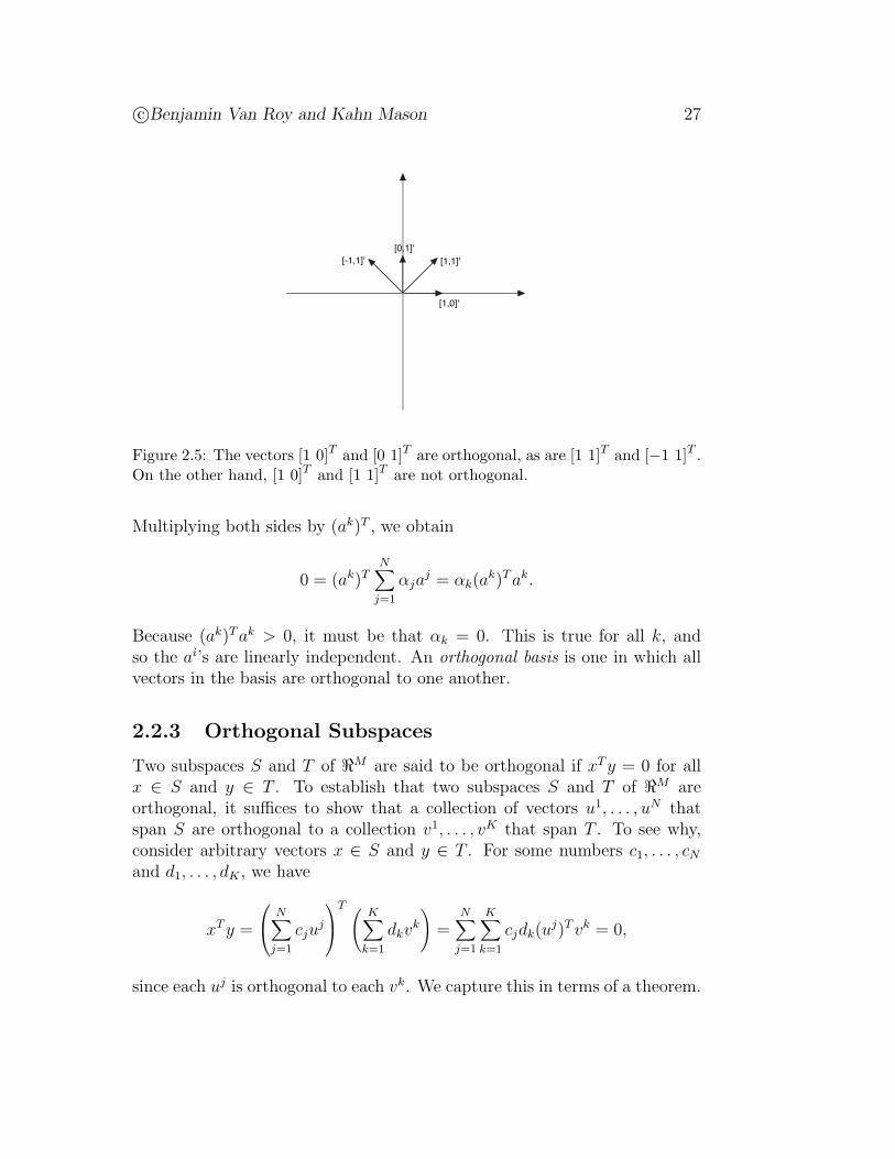
Two vectors x, y $ #M are said to be orthogonal (or perpendicular) if xT y = 0.Figure 2.5 presents four vectors in #2. The vectors [1 0]T and [0 1]T areorthogonal, as are [1 1]T and [!1 1]T . On the other hand, [1 0]T and [1 1]T
are not orthogonal.Any collection of nonzero vectors a1, . . . , aN that are orthogonal to one
another are linearly independent. To establish this, suppose that they areorthogonal, and that
N,
j=1
!jaj = 0.
c"Benjamin Van Roy and Kahn Mason 27
[1,0]'
[1,1]'[0,1]'
[-1,1]'
Figure 2.5: The vectors [1 0]T and [0 1]T are orthogonal, as are [1 1]T and [!1 1]T .On the other hand, [1 0]T and [1 1]T are not orthogonal.
Multiplying both sides by (ak)T , we obtain
0 = (ak)TN,
j=1
!jaj = !k(a
k)T ak.
Because (ak)T ak > 0, it must be that !k = 0. This is true for all k, andso the ai’s are linearly independent. An orthogonal basis is one in which allvectors in the basis are orthogonal to one another.
2.2.3 Orthogonal Subspaces
Two subspaces S and T of #M are said to be orthogonal if xT y = 0 for allx $ S and y $ T . To establish that two subspaces S and T of #M areorthogonal, it su"ces to show that a collection of vectors u1, . . . , uN thatspan S are orthogonal to a collection v1, . . . , vK that span T . To see why,consider arbitrary vectors x $ S and y $ T . For some numbers c1, . . . , cN
and d1, . . . , dK , we have
xT y =
4
5N,
j=1
cjuj
6
7T 8
K,
k=1
dkvk
9
=N,
j=1
K,
k=1
cjdk(uj)T vk = 0,
since each uj is orthogonal to each vk. We capture this in terms of a theorem.
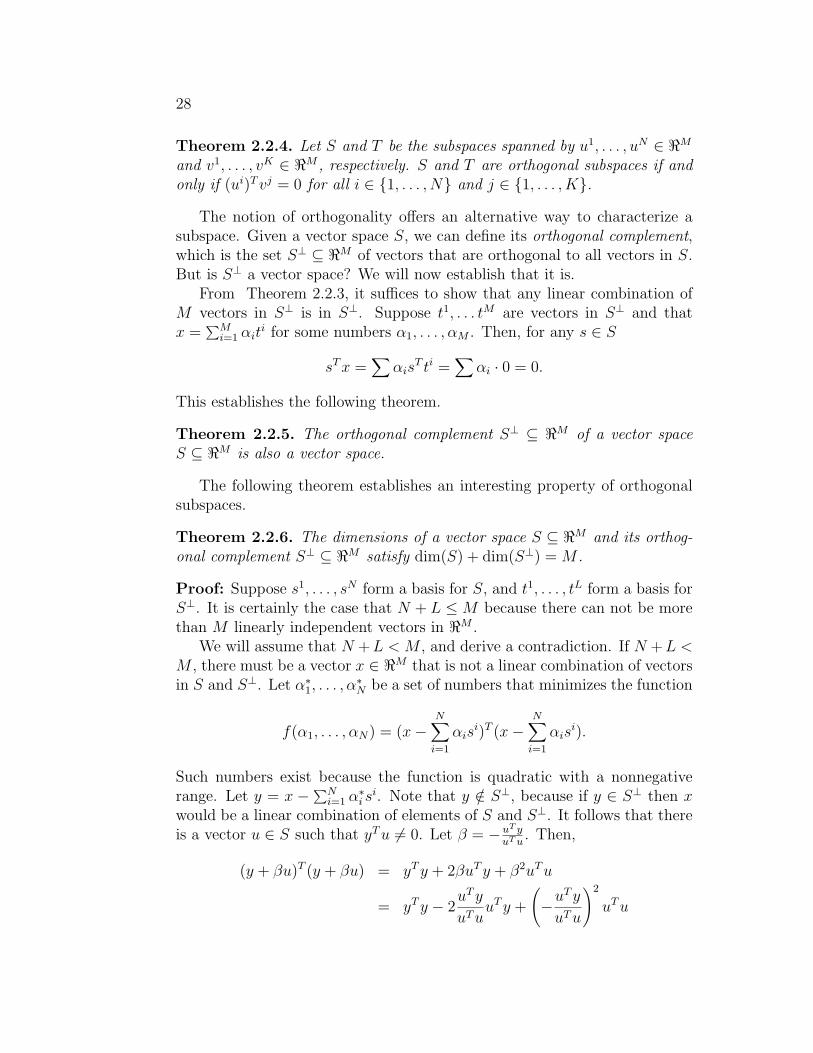
28
Theorem 2.2.4. Let S and T be the subspaces spanned by u1, . . . , uN $ #M
and v1, . . . , vK $ #M , respectively. S and T are orthogonal subspaces if andonly if (ui)T vj = 0 for all i $ {1, . . . , N} and j $ {1, . . . , K}.
The notion of orthogonality o!ers an alternative way to characterize asubspace. Given a vector space S, we can define its orthogonal complement,which is the set S$ ( #M of vectors that are orthogonal to all vectors in S.But is S$ a vector space? We will now establish that it is.
From Theorem 2.2.3, it su"ces to show that any linear combination ofM vectors in S$ is in S$. Suppose t1, . . . tM are vectors in S$ and thatx =
)Mi=1 !iti for some numbers !1, . . . ,!M . Then, for any s $ S
sT x =,
!isT ti =
,!i · 0 = 0.
This establishes the following theorem.
Theorem 2.2.5. The orthogonal complement S$ ( #M of a vector spaceS ( #M is also a vector space.
The following theorem establishes an interesting property of orthogonalsubspaces.
Theorem 2.2.6. The dimensions of a vector space S ( #M and its orthog-onal complement S$ ( #M satisfy dim(S) + dim(S$) = M .
Proof: Suppose s1, . . . , sN form a basis for S, and t1, . . . , tL form a basis forS$. It is certainly the case that N + L ) M because there can not be morethan M linearly independent vectors in #M .
We will assume that N + L < M , and derive a contradiction. If N + L <M , there must be a vector x $ #M that is not a linear combination of vectorsin S and S$. Let !"1, . . . ,!
"N be a set of numbers that minimizes the function
f(!1, . . . ,!N) = (x!N,
i=1
!isi)T (x!
N,
i=1
!isi).
Such numbers exist because the function is quadratic with a nonnegativerange. Let y = x !)N
i=1 !"i si. Note that y /$ S$, because if y $ S$ then x
would be a linear combination of elements of S and S$. It follows that thereis a vector u $ S such that yT u '= 0. Let " = !uT y
uT u . Then,
(y + "u)T (y + "u) = yT y + 2"uT y + "2uT u
= yT y ! 2uT y
uT uuT y +
8
!uT y
uT u
92
uT u

c"Benjamin Van Roy and Kahn Mason 29
= yT y ! 2(uT y)2
uT u+
(uT y)2
uT u
= yT y ! (uT y)2
uT u< yT y
which contradicts that fact that yT y is the minimum of f(!1, . . . ,!N). Itfollows that N + L = M .
2.2.4 Vector Spaces Associated with Matrices
Given a matrix A $ #M!N , there are several subspaces of #M and #N worthstudying. An understanding of these subspaces facilitates intuition aboutlinear systems of equations. The first of these is the subspace of #M spannedby the columns of A. This subspace is called the column space of A, and wedenote it by C(A). Note that, for any vector x $ #N , the product Ax is inC(A), since it is a linear combination of columns of A:
Ax =N,
j=1
xjA"j.
The converse is also true. If b $ #M is in C(A) then there is a vector x $ #N
such that Ax = b.The row space of A is the subspace of #N spanned by the rows of A. It
is equivalent to the column space C(AT ) of AT . If a vector c $ #N is in therow space of A then there is a vector y $ #M such that AT y = c or, writtenin another way, yT A = cT .
Another interesting subspace of #N is the null space. This is the set ofvectors x $ #N such that Ax = 0. Note that the null space is the set ofvectors that are orthogonal to every row of A. Hence, by Theorem 2.2.4, thenull space is the orthogonal complement of the row space. We denote thenull space of a matrix A by N (A).
The left null space is analogously defined as the set of vectors y $ #M
such that yT A = 0, or written in another way, AT y = 0. Again, by Theorem2.2.4, the left null space is the set of vectors that are orthogonal to everycolumn of A and is equivalent to N (AT ), the null space of AT . The followingtheorem summarizes our observations relating null spaces to row and columnspaces.
Theorem 2.2.7. The left null space is the orthogonal complement of thecolumn space. The null space is the orthogonal complement of the row space.
30
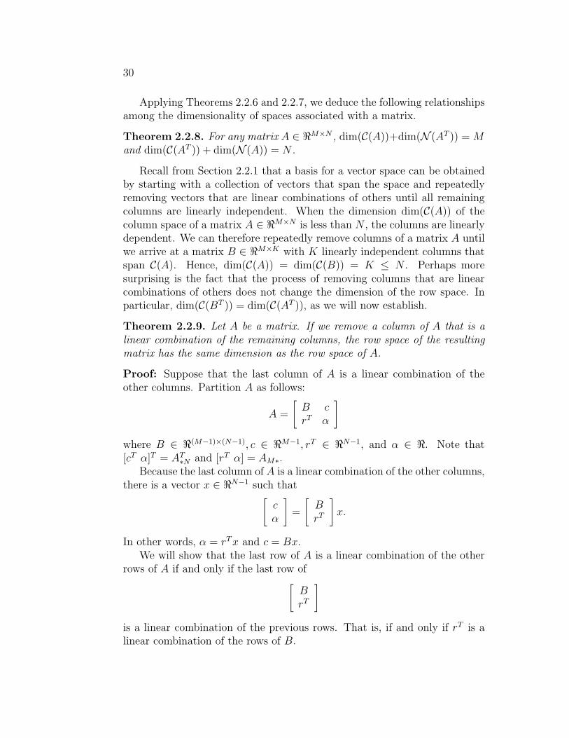
Applying Theorems 2.2.6 and 2.2.7, we deduce the following relationshipsamong the dimensionality of spaces associated with a matrix.
Theorem 2.2.8. For any matrix A $ #M!N , dim(C(A))+dim(N (AT )) = Mand dim(C(AT )) + dim(N (A)) = N .
Recall from Section 2.2.1 that a basis for a vector space can be obtainedby starting with a collection of vectors that span the space and repeatedlyremoving vectors that are linear combinations of others until all remainingcolumns are linearly independent. When the dimension dim(C(A)) of thecolumn space of a matrix A $ #M!N is less than N , the columns are linearlydependent. We can therefore repeatedly remove columns of a matrix A untilwe arrive at a matrix B $ #M!K with K linearly independent columns thatspan C(A). Hence, dim(C(A)) = dim(C(B)) = K ) N . Perhaps moresurprising is the fact that the process of removing columns that are linearcombinations of others does not change the dimension of the row space. Inparticular, dim(C(BT )) = dim(C(AT )), as we will now establish.
Theorem 2.2.9. Let A be a matrix. If we remove a column of A that is alinear combination of the remaining columns, the row space of the resultingmatrix has the same dimension as the row space of A.
Proof: Suppose that the last column of A is a linear combination of theother columns. Partition A as follows:
A =
'B crT !
(
where B $ #(M#1)!(N#1), c $ #M#1, rT $ #N#1, and ! $ #. Note that[cT !]T = AT
"N and [rT !] = AM".Because the last column of A is a linear combination of the other columns,
there is a vector x $ #N#1 such that'
c!
(
=
'BrT
(
x.
In other words, ! = rT x and c = Bx.We will show that the last row of A is a linear combination of the other
rows of A if and only if the last row of'
BrT
(
is a linear combination of the previous rows. That is, if and only if rT is alinear combination of the rows of B.
c"Benjamin Van Roy and Kahn Mason 31
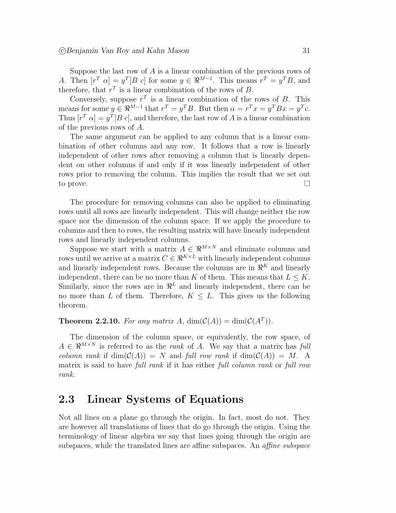
Suppose the last row of A is a linear combination of the previous rows ofA. Then [rT !] = yT [B c] for some y $ #M#1. This means rT = yT B, andtherefore, that rT is a linear combination of the rows of B.
Conversely, suppose rT is a linear combination of the rows of B. Thismeans for some y $ #M#1 that rT = yT B. But then ! = rT x = yT Bx = yT c.Thus [rT !] = yT [B c], and therefore, the last row of A is a linear combinationof the previous rows of A.
The same argument can be applied to any column that is a linear com-bination of other columns and any row. It follows that a row is linearlyindependent of other rows after removing a column that is linearly depen-dent on other columns if and only if it was linearly independent of otherrows prior to removing the column. This implies the result that we set outto prove.
The procedure for removing columns can also be applied to eliminatingrows until all rows are linearly independent. This will change neither the rowspace nor the dimension of the column space. If we apply the procedure tocolumns and then to rows, the resulting matrix will have linearly independentrows and linearly independent columns.
Suppose we start with a matrix A $ #M!N and eliminate columns androws until we arrive at a matrix C $ #K!L with linearly independent columnsand linearly independent rows. Because the columns are in #K and linearlyindependent, there can be no more than K of them. This means that L ) K.Similarly, since the rows are in #L and linearly independent, there can beno more than L of them. Therefore, K ) L. This gives us the followingtheorem.
Theorem 2.2.10. For any matrix A, dim(C(A)) = dim(C(AT )).
The dimension of the column space, or equivalently, the row space, ofA $ #M!N is referred to as the rank of A. We say that a matrix has fullcolumn rank if dim(C(A)) = N and full row rank if dim(C(A)) = M . Amatrix is said to have full rank if it has either full column rank or full rowrank.
2.3 Linear Systems of Equations
Not all lines on a plane go through the origin. In fact, most do not. Theyare however all translations of lines that do go through the origin. Using theterminology of linear algebra we say that lines going through the origin aresubspaces, while the translated lines are a"ne subspaces. An a!ne subspace
32
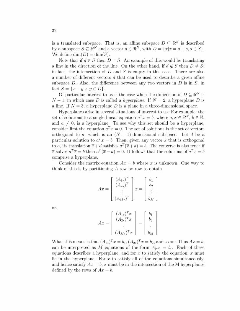
is a translated subspace. That is, an a"ne subspace D ( #N is describedby a subspace S ( #N and a vector d $ #N , with D = {x|x = d + s, s $ S}.We define dim(D) = dim(S).
Note that if d $ S then D = S. An example of this would be translatinga line in the direction of the line. On the other hand, if d /$ S then D '= S;in fact, the intersection of D and S is empty in this case. There are alsoa number of di!erent vectors d that can be used to describe a given a"nesubspace D. Also, the di!erence between any two vectors in D is in S, infact S = {x! y|x, y $ D}.
Of particular interest to us is the case when the dimension of D ( #N isN ! 1, in which case D is called a hyperplane. If N = 2, a hyperplane D isa line. If N = 3, a hyperplane D is a plane in a three-dimensional space.
Hyperplanes arise in several situations of interest to us. For example, theset of solutions to a single linear equation aT x = b, where a, x $ #N , b $ #,and a '= 0, is a hyperplane. To see why this set should be a hyperplane,consider first the equation aT x = 0. The set of solutions is the set of vectorsorthogonal to a, which is an (N ! 1)-dimensional subspace. Let d be aparticular solution to aT x = b. Then, given any vector x that is orthogonalto a, its translation x+d satisfies aT (x+d) = b. The converse is also true: ifx solves aT x = b then aT (x! d) = 0. It follows that the solutions of aT x = bcomprise a hyperplane.
Consider the matrix equation Ax = b where x is unknown. One way tothink of this is by partitioning A row by row to obtain
Ax =
!
""""#
(A1")T
(A2")T
...(AM")T
$
%%%%&x =
!
""""#
b1
b2...
bM
$
%%%%&
or,
Ax =
!
""""#
(A1")T x(A2")T x
...(AM")T x
$
%%%%&=
!
""""#
b1
b2...
bM
$
%%%%&
What this means is that (A1")T x = b1, (A2")T x = b2, and so on. Thus Ax = b,can be interpreted as M equations of the form Ai"x = bi. Each of theseequations describes a hyperplane, and for x to satisfy the equation, x mustlie in the hyperplane. For x to satisfy all of the equations simultaneously,and hence satisfy Ax = b, x must be in the intersection of the M hyperplanesdefined by the rows of Ax = b.
c"Benjamin Van Roy and Kahn Mason 33
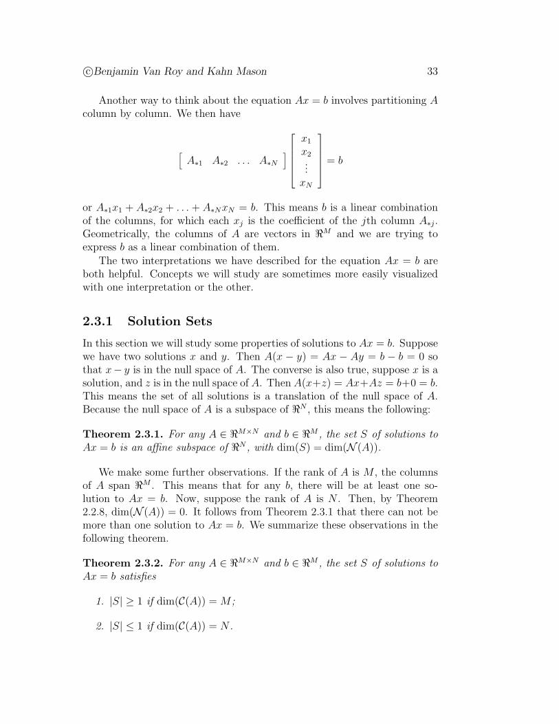
Another way to think about the equation Ax = b involves partitioning Acolumn by column. We then have
*A"1 A"2 . . . A"N
+
!
""""#
x1
x2...
xN
$
%%%%&= b
or A"1x1 + A"2x2 + . . . + A"NxN = b. This means b is a linear combinationof the columns, for which each xj is the coe"cient of the jth column A"j.Geometrically, the columns of A are vectors in #M and we are trying toexpress b as a linear combination of them.
The two interpretations we have described for the equation Ax = b areboth helpful. Concepts we will study are sometimes more easily visualizedwith one interpretation or the other.
2.3.1 Solution Sets
In this section we will study some properties of solutions to Ax = b. Supposewe have two solutions x and y. Then A(x ! y) = Ax ! Ay = b ! b = 0 sothat x! y is in the null space of A. The converse is also true, suppose x is asolution, and z is in the null space of A. Then A(x+z) = Ax+Az = b+0 = b.This means the set of all solutions is a translation of the null space of A.Because the null space of A is a subspace of #N , this means the following:
Theorem 2.3.1. For any A $ #M!N and b $ #M , the set S of solutions toAx = b is an a!ne subspace of #N , with dim(S) = dim(N (A)).
We make some further observations. If the rank of A is M , the columnsof A span #M . This means that for any b, there will be at least one so-lution to Ax = b. Now, suppose the rank of A is N . Then, by Theorem2.2.8, dim(N (A)) = 0. It follows from Theorem 2.3.1 that there can not bemore than one solution to Ax = b. We summarize these observations in thefollowing theorem.
Theorem 2.3.2. For any A $ #M!N and b $ #M , the set S of solutions toAx = b satisfies
1. |S| * 1 if dim(C(A)) = M ;
2. |S| ) 1 if dim(C(A)) = N .
34
Given a matrix A $ #M!N , we can define a function f(x) = Ax, mapping#N to #M . The range of this function is the column space of A. If we restrictthe domain to the row space of A, the function is a one-to-one mapping fromrow space to column space, as captured by the following theorem.
Theorem 2.3.3. For any matrix A $ #M!N , the function f(x) = Ax is aone-to-one mapping from the row space of A to the column space of A.
Proof: Since the columns of A span the column space, the range of f isthe column space. Furthermore, each vector in the column space is givenby f(x) $ #M for some x $ C(AT ). This is because any such y $ #N canbe written as y = x + z for some x $ C(AT ) and z $ N (A), so f(y) =A(x + z) = Ax = f(x). To complete the proof, we need to establish thatonly one element of the row space can map to any particular element of thecolumn space.
Suppose that for two vectors x1, x2 $ C(AT ), both in the row space ofA, we have Ax1 = Ax2. Because x1 and x2 are in the row space of A,there are vectors y1, y2 $ #M such that x1 = AT y1 and x2 = AT y2. Itfollows that AAT y1 = AAT y2, or AAT (y1 ! y2) = 0. This implies that(y1 ! y2)T AAT (y1 ! y2) = 0. This is the square of the norm of AT (y1 ! y2),and the fact that it is equal to zero implies that AT (y1 ! y2) = 0. Hence,x1 ! x2 = 0, or x1 = x2. The result follows
2.3.2 Matrix Inversion
Given a matrix A $ #M!N , a matrix B $ #N!M is said to be a left inverse ofA if BA = I. Analogously, a matrix B $ #N!M is said to be a right inverseof A if AB = I. A matrix cannot have both a left inverse and a right inverseunless both are equal. To see this, suppose that the left inverse of A is Band that the right inverse is C. We would then have
B = B(AC) = (BA)C = C.
Note that if N '= M , A cannot have both a left inverse and a rightinverse. This is because the left inverse is in #N!M , while the right inverseis in #M!N , so they cannot possibly be equal. Hence, only square matricescan have both left and right inverses. If A is a square matrix, any left inversemust be equal to any right inverse. So when a left and right inverse exists,there is a single matrix that is simultaneously the unique left inverse and theunique right inverse. This matrix is simply referred to as the inverse, anddenoted by A#1.
c"Benjamin Van Roy and Kahn Mason 35
How do we find inverses of a matrix A $ #M!N? To find a right inverse B,so that AB = I, we can partition the matrix B into columns [B"1 · · · B"M ]and I into columns [e1 · · · eM ], and solve AB"j = ej to find each jth columnof B. Therefore, the matrix A has a right inverse if and only if each ej is inits column space. Since the vectors e1, . . . , eN span #M , the column space ofA must be #M . Hence, A has a right inverse if and only if it has rank M –in other words, full row rank.
For left inverses, the picture is similar. We first transpose the equationBA = I to get AT BT = IT = I, then partition by column as we did to find aright inverse. Now we see that A has a left inverse if and only if its row spaceis #N . Hence, A has a left inverse if and only if it has full column rank.
We summarize our observations in the following theorem.
Theorem 2.3.4. For any matrix A,(a) A has a right inverse if and only if it has full row rank;(b) A has a left inverse if and only if it has full column rank;(c) if A has full rank, then it has at least one left inverse or right inverse;(d) if A is square and has full rank, then A has an inverse, which is unique.
Note, that in Theorem 2.3.3, we described a function defined by A, andsaw that it was a one-to-one mapping from the row space to the columnspace. If A is has an inverse, then the column space and the row space willboth be #N (remember that A must be square). This gives us the following.
Theorem 2.3.5. Let f(x) = Ax for a matrix A $ #M!N . Then, f is a one-to-one mapping from #N to #M if and only if A has an inverse. Furthermore,this can only be the case if N = M .
One final note on inverses, if A has an inverse then so does AT , and in fact,(AT )#1 = (A#1)T . This is verified by simply multiplying the two together(AT )(A#1)T = (A#1A)T = IT = I, and the check for left inverse is similar.To simplify notation, the inverse of a transpose is often denoted as A#T .
2.4 Contingent Claims
Prices of assets traded in public exchanges fluctuate over time. If we makean investment today, our payo! is subject to future market prices. Manytimes we consider assets whose payo!s are completely determined by otherassets. We refer to these as derivative assets.
For example, we might consider corporate stock, as being fundamental – astock’s value is derived from the state of a company and market expectationsabout its future. Other assets – known as derivatives – are contracts that

36
promise payo!s that are functions of the future price of other assets. In asense, these assets are synthetic.
Whether fundamental or synthetic, assets traded in a market can bethought of abstractly as contingent claims. This term refers to the fact thatthe future payo! from an asset is contingent on the future state of variablesdictated by the market. We present some common examples of contingentclaims.
Example 2.4.1. (Stocks, Bonds, and Options) We describe four types ofcontingent claims. A share of corporate stock entitles its holder to a fractionof the company’s value. This value is determined by the market. A zero-coupon bond is a contract that o"ers the holder a $1 payo" on some futuredate, referred to as the maturity date, specified by terms of the contract. AEuropean put option is a contract that o"ers its holder the option to sell ashare of stock to the grantor at a particular price, referred to as the strikeprice, on an particular future date, referred to as the expiration date. Thestrike price and expiration date are specified by terms of the contract. AEuropean call option, on the other hand, o"ers its holder the option to buya share of stock from the grantor at a strike price on an expiration date.
Consider four assets: a share of stock, a zero-coupon bond maturing inone year, and European put and call options on the stock, both expiring in oneyear, with strike prices of $40 and $60. We could purchase any combinationof these assets today and liquidate in one year to receive a payo". The payo"of each asset will only depend on the price of the stock one year from now.Hence, we can visualize the payo" in terms of a function mapping the stockprice one year from now to the associated payo" from the asset. Figure 2.6illustrates the payo" functions associated with each asset.
Each payo" function provides the value of one unit of an asset one yearfrom now, as a function of the stock price. In the case of the stock, the valueis the stock price itself. For the put, we would exercise our option to sell thestock only if the the strike price exceeds the stock price. In this event, wewould purchase a share of stock at the prevailing stock price and sell it at thestrike price of $40, keeping the di"erence as a payo". If the stock price exceedsthe strike price, we would discard the contract without exercising. The storyis similar for the call, except that we would only exercise our option to buyif the stock price exceeds the strike price. In this event, we would purchaseone share of stock at the strike price of $60 and sell it at the prevailing stockprice, keeping the di"erence as a payo".
Suppose that the price of the stock in the preceding example can onlytake on values in {1, . . . , 100} a year from now. Then, payo! functions areconveniently represented in terms of payo" vectors. For example, the payo!

c"Benjamin Van Roy and Kahn Mason 37
stockprice
payoff
20 40 60 80 100 stockprice
payoff
20 40 60 80 100
(a) (b)
stockprice
payoff
20 40 60 80 100 stockprice
payoff
20 40 60 80 100
(c) (d)
Figure 2.6: Payo! functions of a share of stock (a), a zero-coupon bond (b), aEuropean put option (c), and a European call option (d).
vector a1 $ #100 for the stock would be defined by a1i = i. Similarly, the
payo! vectors for the zero-coupon bond, European put option, and Europeancall option would be a2
i = 1, a3i = max(40 ! i, 0), and a4
i = max(i ! 60, 0),respectively.
More generally, we may be concerned with large numbers of assets drivenby many market prices – perhaps even the entire stock market. Even insuch cases, the vector representation applies, so long as we enumerate allpossible outcomes of interest. In particular, given a collection of N assetsand M possible outcomes for relevant market prices, the payo! functionassociated with any asset j $ {1, . . . , N} can be thought of as a payo! vectoraj $ #M , where each ith component is the payo! of the asset in outcomei $ {1, . . . ,M}.
It is sometimes convenient to represent payo! vectors for all assets interms of a single matrix. Each column of this payo" matrix P is the payo!
38
vector for an asset. In particular,
P =*
a1 . . . aN+.
2.4.1 Structured Products and Market Completeness
Investment banks serve investors with specialized needs. One service o!eredby some banks involves structuring and selling assets that accommodate acustomer’s demands. Such assets are called structured products. We providea simple example.
Example 2.4.2. (Currency Hedge) A company is planning to set up mar-keting operations in a foreign country. It is motivated by favorable sales pro-jections. However, the company faces significant risks that are unrelated to itsproducts or operation. If the Dollar value of the foreign currency depreciates,it may operate at a loss even if sales projections are met. In addition, if theeconomy of the country is unstable, there may be a dramatic devaluation aris-ing from poor economic conditions. In this event, the sales projections wouldbecome infeasible and the company would pull out of the country entirely.
The anticipated profit over the coming year from operating in this foreigncountry is p Dollars, so long as the Dollar value of the currency remains atits current level of r0. However, if the Dollar value were to change to r1, thecompany’s anticipated profit would become pr1/r0. If the exchange rate dropsto a critical value of r1 = r", the company would shut down operations andpull out of the country entirely. The anticipated profit over the coming yearas a function of the exchange rate is illustrated in Figure 2.7(a).
The company consults with an investment bank, expressing a desire tomeet its profit projection during its first year of operation by focusing onproduct sales, without having to face risks associated with the country’s cur-rency and economic conditions. The bank designs a structured product thato"ers a payo" in one year that is contingent on the prevailing exchange rater1. The payo" function is illustrated in Figure 2.7(b). By purchasing thisstructured product, the company can rest assured that its profit over the com-ing year from this foreign operation will be p Dollars, so long as its salesprojections are met.
When selling a structured product, an investment bank may be taking onsignificant risks. For example, if the country discussed in the above exampleturns out to have an economic crisis, the bank will owe a large sum of moneyto the company. This risk can be avoided, however, if the bank is able toreplicate the structured product. It is said that a structured product with a

c"Benjamin Van Roy and Kahn Mason 39
profit
r1r * r0
p
payoff
r1r * r0
p
(a) (b)
Figure 2.7: (a) A company’s profit as a function of the exchange rate. (b) Thepayo! function for a protective structured product.
payo! vector b $ #M can be replicated with assets available in the market if
Px = b,
for some x $ #N . In financial terms, x represents a portfolio that can beacquired by trading in the market, and Px is the payo! vector associatedwith this portfolio. Each nonnegative xj represents a number of units of thejth asset held in the portfolio. Each negative xj represents a quantity soldshort. The term short-sell refers to a process whereby one borrows unitsof an asset from a broker, sells them, and returns them to the broker at alater time after buying an equal number of units of the same asset from themarket.
If Px = b, the payo! from the portfolio equals that of the structuredproduct in every possible future outcome. Hence, by acquiring the portfoliowhen selling the structured product, the bank mitigates all risk. It is simplyintermediating between the market and its customer. To do this right, thebank must solve the equation Px = b.
Can every possible contingent claim be replicated by assets available inthe market? To answer this question, recall that, by definition, a contingentclaim with payo! function b $ #M can be replicated if and only if Px = bfor some x. Hence, to replicate every possible contingent claim, Px = b musthave a solution for every b $ #M . This is true only if C(P ) = #M . In thisevent, the market is said to be complete – that is, any new asset that mightbe introduced to the market can be replicated by existing assets.

40
2.4.2 Pricing and Arbitrage
Until now, we have focussed on payo!s – what we can make from investingin assets. We now bring attention to prices – what we have to pay for assets.Let us represent initial prices of assets in the market by a vector # $ #N .Hence, the unit cost of asset j is #j and a portfolio x $ #N requires aninvestment of #T x.
How should an investment bank price a structured product? The an-swer seems clear: since the investment bank is replicating the product usinga portfolio, the bank should think of the price as being equal that of theportfolio. Of course, the bank will also tack on a premium to generate someprofit.
If an asset in the market can be replicated by others, this should alsotranslate to a price relationship. In particular, the price of a replicatingportfolio should equal that of the replicated asset. If it were greater, onecould short-sell the portfolio and purchase the asset to generate immediateprofits without incurring cost or risk. Similarly, if the price of the replicatingportfolio were lower than that of the asset, one would short sell the assetand purchase the portfolio. In either case, the initial investment is negative(the individual carrying out the transactions receives money) and the futurepayo! is zero, regardless of the outcome.
What we have just described is an arbitrage opportunity. More generally,an arbitrage opportunity is an investment strategy that involves a negativeinitial investment and guarantees a nonnegative payo!. In mathematicalterms, an arbitrage opportunity is represented by a portfolio x $ #N suchthat #T x < 0 and Px * 0. Under the assumption that arbitrage opportuni-ties do not exist, it often possible to derive relationships among asset prices.We provide a simple example
Example 2.4.3. (Put-Call Parity) Consider four assets:(a) a stock currently priced at s0 that will take on a price s1 $ {1, . . . , 100}one month from now;(b) a zero-coupon bond priced at "0, maturing one month from now;(c) a European put option currently priced at p0 with a strike price $ > 0,expiring one month from now;(d) a European call option currently priced at c0 with the same strike price$, expiring one month from now.
The payo" vectors a1, a2, a3, a4 $ #M are given by
a1i = µi, a2
i = 1, a3i = max($! µi, 0), a4
i = max(µi ! $, 0),

c"Benjamin Van Roy and Kahn Mason 41
for i $ {1, . . . ,M}. Note that if we purchase one share of the stock and oneput option and short-sell one call option and $ units of the bond, we areguaranteed zero payo"; i.e.,
a1 ! $a2 + a3 ! a4 = 0.
The initial investment in this portfolio would be
s0 ! $"0 + p0 ! c0.
If this initial investment is nonzero, there would be an arbitrage opportu-nity. Hence, in the absence of arbitrage opportunities, we have the pricingrelationship
s0 ! $"0 + p0 ! c0 = 0,
which is known as the put-call parity.
Because arbitrage opportunities are lucrative, one might wish to deter-mine whether they exist. In fact, one might consider writing a computerprogram that automatically detects such opportunities whenever they areavailable. We have not yet developed the tools to do this – but we will.In particular, linear programming o!ers a solution to this problem. Linearprogramming will also o!er an approach to mitigating risk and pricing whenselling structured products that can not be replicated by assets in the market.Duality theory will also o!er interesting insights about pricing contingentclaims in the absence of arbitrage opportunities. So the story of contingentclaims and arbitrage is not over but to be continued in subsequent chapters.
2.5 Exercises
Question 1
Let a = [1, 2]T and b = [2, 1]T . On the same graph, draw each of the following
1. The set of all points x $ #2 that satisfy aT x = 0.
2. The set of all points x $ #2 that satisfy aT x = 1.
3. The set of all points x $ #2 that satisfy bT x = 0.
4. The set of all points x $ #2 that satisfy bT x = 1.
5. The set all points x $ #2 that satisfy [a b]x = [0, 1]T .
6. The set all points x $ #2 that satisfy [a b]x = [0, 2]T .
In addition, shade the region that consists of all x $ #2 that satisfyaT x ) 0.

42
Question 2
Consider trying to solve Ax = b where
A =
!
"#1 20 32 !1
$
%&
1. Find a b so that Ax = b has no solution.
2. Find a non-zero b so that Ax = b has a solution.
Question 3
Find two x $ #4 that solve all of the following equations.
[0, 2, 0, 0] x = 4
[1, 0, 0, 0] x = 3
[2,!1,!2, 1] x = 0
Write [4, 3, 0]T as a linear combination of [0, 1, 2]T , [2, 0,!1]T , [0, 0,!2]T
and [0, 0, 1]T in two di!erent ways. Note: When we say write x as a linearcombination of a, b and c, what we mean is find the coe"cients of the a, band c. For example x = 5a! 2b + c.
Question 4
Suppose A, B $ #3!3 are defined by Aij = i + j and Bij = (!1)ij for each iand j. What is AT ? AB?
Suppose we now change some elements of A so that A1j = ej1. What is
A now?
Question 5
Suppose U and V are both subspaces of S. Are U+V and U,V subspaces ofS? Why, or why not? Hint: Think about whether or not linear combinationsof vectors are still in the set.
c"Benjamin Van Roy and Kahn Mason 43
Question 6
a =
!
""""""#
14!123
$
%%%%%%&, b =
!
""""""#
120!31
$
%%%%%%&, c =
!
""""""#
02!152
$
%%%%%%&, d =
!
""""""#
102!8!1
$
%%%%%%&, e =
!
""""""#
110!1179
$
%%%%%%&, f =
!
""""""#
!4!21.5272
$
%%%%%%&
1. The span of {a, b, c} is an N dimensional subspace of #M . What areM and N?
2. What is 6a + 5b! 3e + 2f?
3. Write a as a linear combination of b, e, f .
4. write f as a linear combination of a, b, e.
5. The span of {a, b, c, d, e, f} is an N dimensional subspace of #M . Whatare M and N?
Question 7
Suppose I have 3 vectors x, y and z. I know xT y = 0 and that y is not amultiple of z. Is it possible for {x, y, z} to be linearly dependent? If so, givean example. If not, why not?.
Question 8
Find 2 matrices A, B $ #2!2 so that none of the entries in A or B are zero,but AB is the zero matrix. Hint: Orthogonal vectors.
Question 9
Suppose the only solution to Ax = 0 is x = 0. If A $ #M!N what is its rank,and why?
Question 10
The system of equations
3x + ay = 0
ax + 3y = 0
44
always has as a solution x = y = 0. For some a the equations have morethan one solution. Find two such a.
Question 11
In #3, describe the 4 subspaces (column, row, null, left-null) of the matrix
A =
!
"#0 1 00 0 10 0 0
$
%&
Question 12
In real life there are many more options than those described in class, andthey can have di!ering expiry dates, strike prices, and terms.
1. Suppose there are 2 call options with strike prices $ 1 and $ 2. Whichof the two will have the higher price?
2. Suppose the options were put options. Which would now have thehigher price?
3. If an investor thinks that the market will be particularly volatile in thecoming weeks, but does not know whether the market will go up ordown, they may choose to buy an option that pays |S ! K| where Swill be the value of a particular share in one months time, and K is thecurrent price of the share. If the price of a zero coupon bond maturingin one month is 1, then what is the di!erence between a call option anda put option both having strike price K. (Report the answer in termsof the strike price K.)
4. Suppose I am considering buying an option on a company. I am consid-ering options with a strike price of $ 100, but there are di!erent expirydates. The call option expiring in one month costs $ 10 while the putoption expiring in one month costs $ 5. If the call option expiring intwo months costs $ 12 and zero coupon bonds for both time framescost $ 0.8, then how much should a put option expiring in two monthscost?
Question 13
Find a matrix whose row space contains [1 2 1]T and whose null space contains[1 ! 2 1]T or show that there is no such matrix.

c"Benjamin Van Roy and Kahn Mason 45
Question 14
True or False:
1. If U is orthogonal to V then U$ is orthogonal to V $.
2. If U is orthogonal to V and V is orthogonal to W , then it is alwaystrue that U us orthogonal to W .
3. If U is orthogonal to V and V is orthogonal to W , then it is never truethat U us orthogonal to W .
Question 15
Can the null space of AB be bigger than the null space of B? If so, give anexample. If not, why not.
Question 16
Find two di!erent matrices that have the same null, row, column, and left-null spaces.