Embed Size (px)
Citation preview
72 © 2017 Cengage Learning. All Rights Reserved. May not be scanned, copied or duplicated, or posted to a publicly accessible website, in whole or in part.
C H A P T E R 2
Differentiation
Section 2.1 The Derivative and the Slope of a Graph
Skills Warm Up
1. P(3, 1), Q(3, 6)
2 2 3
m = 6 − 1
; m is undefined. 3 − 3
6. lim Δx → 0
3x Δx + 3x(Δx) + (Δx) Δx
Δx 3x2 + 3xΔx + (Δx)2
x = 3 = lim Δx → 0 Δx
2. P(2, 2), Q = (−5, 2) = lim 3x2 + 3xΔx + (Δx)2
Δx → 0
m = 2 − 2
= 0 −5 − 2
= 3x2
m 1
= 1
y − 2 = 0(x − 2) 7. li 0 ( ) 2
y = 2 Δx → x x + Δx x
2 2
3. P(1, 5), Q(4, −1)
8. lim Δx → 0
( x +Δx) − x
Δx
m = −1 − 5
= − 6 = − 2 x 2 + 2 xΔx + (Δx)
2 − x 2
4 − 1 3
y − 5 = −2(x − 1)
y − 5 = − 2x + 2
y = − 2x + 7
4. P(3, 5), Q(−1, − 7)
= lim Δx → 0
= lim
Δx → 0
= lim Δx → 0
Δx
2 xΔx + (Δx)2
Δx
Δx(2 x + Δx) Δx
m = − 7 − 5
= −1 − 3
−12 = 3
− 4
= 2x
9. f (x) = 3x
y − 5 = 3(x − 3)
y = 3x − 4
2
10.
Domain: (−∞, ∞)
f (x) = 1
x − 1
5. lim Δx → 0
2 xΔx + (Δx) =
Δx
lim Δx → 0
Δx(2 x + Δx) Δx
Domain: (−∞, 1) ∪ (1, ∞)
= lim 2 x + Δx Δx → 0
11.
f (x) = 1 x3 − 2x2 + 1 x − 1= 2 x
5 3
Domain: (−∞, ∞)
12. f (x) = 6x
x3 + x
Domain: (−∞, 0) ∪ (0, ∞)
1. y 2.
y
x
x
Full file at https://testbank123.eu/Solutions-Manual-for-Calculus-An-Applied-Approach-10th-Edition-Larson
Full file at https://testbank123.eu/Solutions-Manual-for-Calculus-An-Applied-Approach-10th-Edition-Larson
© 2017 Cengage Learning. All Rights Reserved. May not be scanned, copied or duplicated, or posted to a publicly accessible website, in whole or in part.
.
.
3
3
4
Section 2.1 The De rivativ e and the Slo p e of a Grap h 73
y
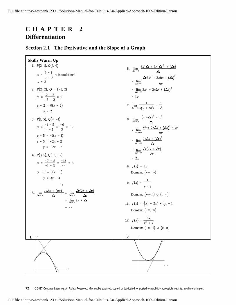
3. 14. 2010: m ≈ 500
2012: m ≈ 500
The slope is the rate of change in millions of dollars
per year of sales for the years 2010 and 2012 for Fossil.
x
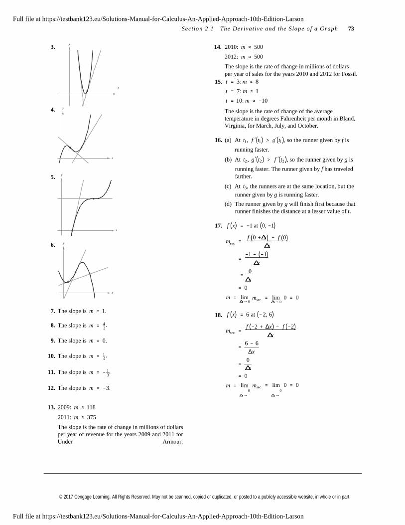
4. y
15. t = 3: m ≈ 8
t = 7: m ≈ 1
t = 10: m ≈ −10
The slope is the rate of change of the average
temperature in degrees Fahrenheit per month in Bland,
Virginia, for March, July, and October.
16. (a) At t1, f ′(t1 ) > g′(t1 ), so the runner given by f is
running faster.
(b) At t2 , g′(t2 ) > f ′(t2 ), so the runner given by g is
5.
y
x
17.
running faster. The runner given by f has traveled
farther.
(c) At t3 , the runners are at the same location, but the
runner given by g is running faster.
(d) The runner given by g will finish first because that
runner finishes the distance at a lesser value of t.
f (x) = −1 at (0, −1)
6. y
msec
f (0 +Δx) − f (0) =
Δx
= −1 − (−1) Δx
= 0 Δx
= 0
m = lim Δx → 0
msec
= lim 0 = 0
Δx → 0
7. The slope is m = 1. 18.
f (x) = 6 at (− 2, 6)
8. The slope is m = 4
msec = f (−2 + Δx) − f (−2)
Δx9. The slope is m = 0.
= 6 − 6
10. The slope is m = 1 Δx
= 0 Δx
11. The slope is m = − 1 . = 0
m = m m
= lim 0 = 0
12. The slope is m = −3. li sec
0 0
Δx → Δx →
13. 2009: m ≈ 118
2011: m ≈ 375
The slope is the rate of change in millions of dollars
per year of revenue for the years 2009 and 2011 for
Under Armour.
Full file at https://testbank123.eu/Solutions-Manual-for-Calculus-An-Applied-Approach-10th-Edition-Larson
Full file at https://testbank123.eu/Solutions-Manual-for-Calculus-An-Applied-Approach-10th-Edition-Larson
© 2017 Cengage Learning. All Rights Reserved. May not be scanned, copied or duplicated, or posted to a publicly accessible website, in whole or in part.
=
=
( )
2 3
( )
x
74 Chapte r 2 Dif ferentiat i on
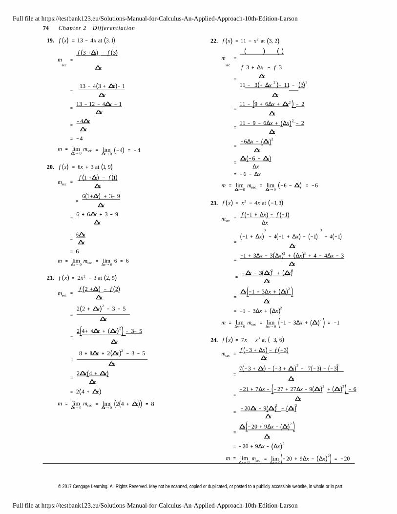
19. f (x) = 13 − 4x at (3, 1) 22. f ( x) = 11 − x2 at (3, 2)
f (3 +Δx) − f (3) m =
( ) ( ) m =
sec Δ
sec f 3 + Δx − f 3
Δx
11 −
3 + Δx 2
− 11 −
3 2
13 − 4(3 + Δ x)− 1
Δ x
= 13 − 12 − 4Δ x − 1
( )
( ) Δx
11 − (9 + 6Δx + Δx 2 ) − 2 =
Δ x
= − 4Δ x Δ x
Δx
11 − 9 − 6Δx + (Δx)2
− 2 =
Δx= − 4
m = lim msec Δx → 0
= lim Δx →0
(− 4) = − 4
− 6Δx − (Δx)2
= Δx
Δx(− 6 − Δx) =
20. f (x) = 6 x + 3 at (1, 9) Δx
= − 6 − Δx
msec
f (1 +Δx) − f (1) =
Δ x
m = lim
Δx →0
msec
= lim Δx →0
(−6 − Δx) = −6
= 6(1 +Δx) + 3− 9
Δ x
23.
f (x) = x3 − 4 x at (−1, 3)
= 6 + 6Δ x + 3 − 9
Δ x
msec
f (−1 + Δx) − f (−1) =
Δx 3 3
= 6Δ x (−1 + Δx) − 4(−1 + Δx) − (−1) − 4(−1)Δ x =
Δx = 6 2 3
m = lim Δx → 0
msec
= lim 6 = 6 Δx → 0
= −1 + 3Δx − 3(Δx) + (Δx) + 4 − 4Δx − 3
Δx 2 3
21. f (x) = 2 x2 − 3 at (2, 5) = −Δx − 3(Δx) + (Δx)
Δx
msec
f (2 +Δx) − f (2) =
Δ x
2(2 + Δ x)2
− 3 − 5
Δx(−1 − 3Δx + (Δx)2 )
= Δx
2
= = −1 − 3Δx + (Δx)Δ x
2(4 + 4Δ x + (Δ x)2 ) − 3− 5
=
m = lim Δx → 0
msec = lim Δx → 0
(−1 − 3Δx + (Δx)2 ) = −1
Δ x 24. f (x) = 7 x − x3 at (− 3, 6)
8 + 8Δ x + 2 Δ x 2
− 3 − 5
= Δ x
msec
f (− 3 + Δx) − f (− 3) =
Δx 3 3
2Δ x(4 + Δ x) =
Δ x
7(− 3 + Δx) − (− 3 + Δx) − 7(− 3) − (− 3) =
Δx
= 2(4 + Δ x) − 21 + 7Δx − (− 27 + 27Δx − 9(Δx) 2
+ (Δx) 3 ) − 6
=
m = lim msec Δx → 0
= lim Δx → 0
(2(4 + Δ x)) = 8 Δx
− 20Δx + 9(Δx) − (Δx) =
Δx
Δx(− 20 + 9Δx − (Δx)2 )
= Δx
= − 20 + 9Δx − (Δx)2
m = lim Δx → 0
msec = lim − 20 + 9Δx − (Δx)2
= − 20 Δx → 0
Full file at https://testbank123.eu/Solutions-Manual-for-Calculus-An-Applied-Approach-10th-Edition-Larson
Full file at https://testbank123.eu/Solutions-Manual-for-Calculus-An-Applied-Approach-10th-Edition-Larson
© 2017 Cengage Learning. All Rights Reserved. May not be scanned, copied or duplicated, or posted to a publicly accessible website, in whole or in part.
Section 2.1 The De rivativ e and the Slo p e of a Grap h 75
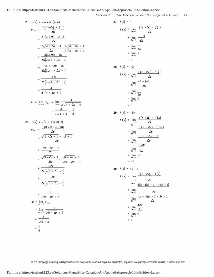
25. f (x) = 2 x at (4, 4) 27. f (x) = 3
msec
f (4 +Δx) − f (4) =
Δx
f ′(x) =
lim Δx → 0
f ( x +Δx) − f ( x) Δx
= 2 4 +Δx − 2 4
Δx
= 2 4 + Δx − 4
⋅ 2 4 + Δx + 4
= lim Δx → 0
= lim Δx → 0
3 − 3
Δx
0
ΔxΔx 2 4 + Δx + 4
= lim 0 4(4+Δx) − 16
= Δx(2 4 + Δx + 4)
= 16 + 4Δx − 16
Δx(2 4 + Δx + 4)
28.
Δx → 0
= 0
f (x) = − 2
f x +Δx − f x
= 4Δx
Δx(2 4 + Δx + 4)
= 4 2 4 + Δx + 4
f ′(x) =
=
=
lim Δx → 0
lim Δx → 0
lim Δx → 0
( ) ( ) Δx
−2 − (−2) Δx
0
Δx
m = lim msec =
lim 4
= lim 0 Δx → 0
Δx →0 Δx →0 2 4 + Δx + 4 = 0
= 4
= 1
2 4 + 4 2 29. f (x) = −5x
26.
f (x) =
x + 1 at (8, 3) f ′(x) =
lim 0
f ( x +Δx) − f ( x) Δx
msec
f (8 +Δx) − f (8) =
Δx
= 8 +Δx + 1 − 8 + 1
Δx
Δx →
= lim Δx → 0
= lim Δx → 0
= lim
−5( x + Δx) − (−5 x) Δx
−5 x − 5Δx + 5 x
Δx
−5Δx
= 9 + Δx − 3 Δx
Δx → 0 Δx
= lim − 5
= 9 +Δx − 3
⋅ 9 + Δx + 3 Δx → 0
Δx
= 9 +Δx − 9
9 + Δx + 3 30.
= −5
f (x) = 4x + 1Δx( 9 + Δx + 3)
′ m f ( x +Δx) − f ( x)
= Δx f (x) = li
0 ΔxΔx( 9 + Δx + 3) Δx →
= lim
4( x +Δx) + 1 − (4 x + 1)
= 1
9 + Δx + 3
Δx → 0
= lim Δx → 0
Δx
4 x + 4Δx + 1 − 4 x − 1
Δxm = lim Δx → 0
= lim
msec
1
= lim
Δx → 0
4Δx
ΔxΔx → 0 9 + Δx + 3 = lim 4
Δx → 0
= 1
= 4 9 + 3
= 1 6
Full file at https://testbank123.eu/Solutions-Manual-for-Calculus-An-Applied-Approach-10th-Edition-Larson
Full file at https://testbank123.eu/Solutions-Manual-for-Calculus-An-Applied-Approach-10th-Edition-Larson
© 2017 Cengage Learning. All Rights Reserved. May not be scanned, copied or duplicated, or posted to a publicly accessible website, in whole or in part.
3
2
3 3
Δs
3 3 3
2 2
− Δt
2 2 2
76 Chapte r 2 Dif ferentiat i on
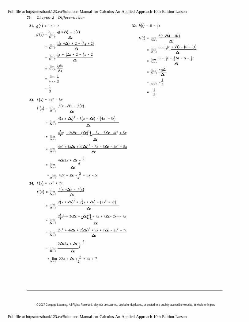
31. g (s) = 1 s + 2 32. h(t ) = 6 − 1 t
g′(s) =
=
=
=
=
lim Δs → 0
lim Δs → 0
lim Δs → 0
lim Δs → 0
lim
g( s+Δs) − g (s) Δs
1 ( s +Δs) + 2 − ( 1 s + 2) Δs
1 s + 1 Δs + 2 − 1 s − 2
Δs
1 3
Δs
1
h′(t ) =
=
=
=
lim Δt → 0
lim Δt → 0
lim Δt → 0
lim Δt → 0
h(t +Δt ) − h(t ) Δt
6 − 1 ( t + Δt ) − (6 − 1 t ) Δt
6 − 1 t − 1 Δt − 6 + 1 t
Δt
1 2
Δt
1Δs → 0 3
= 1
= lim − Δt → 0 2
13 = −
2
33. f (x) = 4 x2 − 5 x
f ′(x) =
=
lim Δ x → 0
lim Δ x → 0
f ( x +Δx) − f ( x) Δ x
4(x + Δ x)2
− 5(x + Δ x) − (4x2 − 5x) Δ x
4( x2 + 2 xΔ x + (Δ x)2 ) − 5x − 5Δ x− 4 x2 + 5x
= lim Δ x → 0 Δ x
= lim
Δ x → 0
= lim
Δ x → 0
4 x2 + 8xΔ x + 4(Δ x)2
− 5x − 5Δ x − 4 x2 + 5x
Δ x
4Δ x 2x + Δ x −
5
4
Δ x
5 = lim 4 2x + Δ x − = 8x − 5 Δ x → 0 4
34. f (x) = 2 x2 + 7 x
f ′(x) =
=
lim Δ x → 0
lim Δ x → 0
f ( x +Δx) − f ( x) Δ x
2(x + Δ x)2
+ 7(x + Δ x) − (2 x2 + 7 x) Δ x
2( x2 + 2 xΔ x + (Δ x)2 ) + 7 x + 7Δ x− 2 x2 − 7 x
= lim Δ x → 0 Δ x
= lim
Δ x → 0
= lim
Δ x → 0
2 x2 + 4 xΔ x + 2(Δ x)2
+ 7 x + 7Δ x − 2 x2 − 7 x
Δ x
2Δ x 2 x + Δ x +
7
2
Δ x
7 = lim 2 2 x + Δ x + = 4 x + 7 Δ x → 0 2
Full file at https://testbank123.eu/Solutions-Manual-for-Calculus-An-Applied-Approach-10th-Edition-Larson
Full file at https://testbank123.eu/Solutions-Manual-for-Calculus-An-Applied-Approach-10th-Edition-Larson
© 2017 Cengage Learning. All Rights Reserved. May not be scanned, copied or duplicated, or posted to a publicly accessible website, in whole or in part.
Section 2.1 The De rivativ e and the Slo p e of a Grap h 77
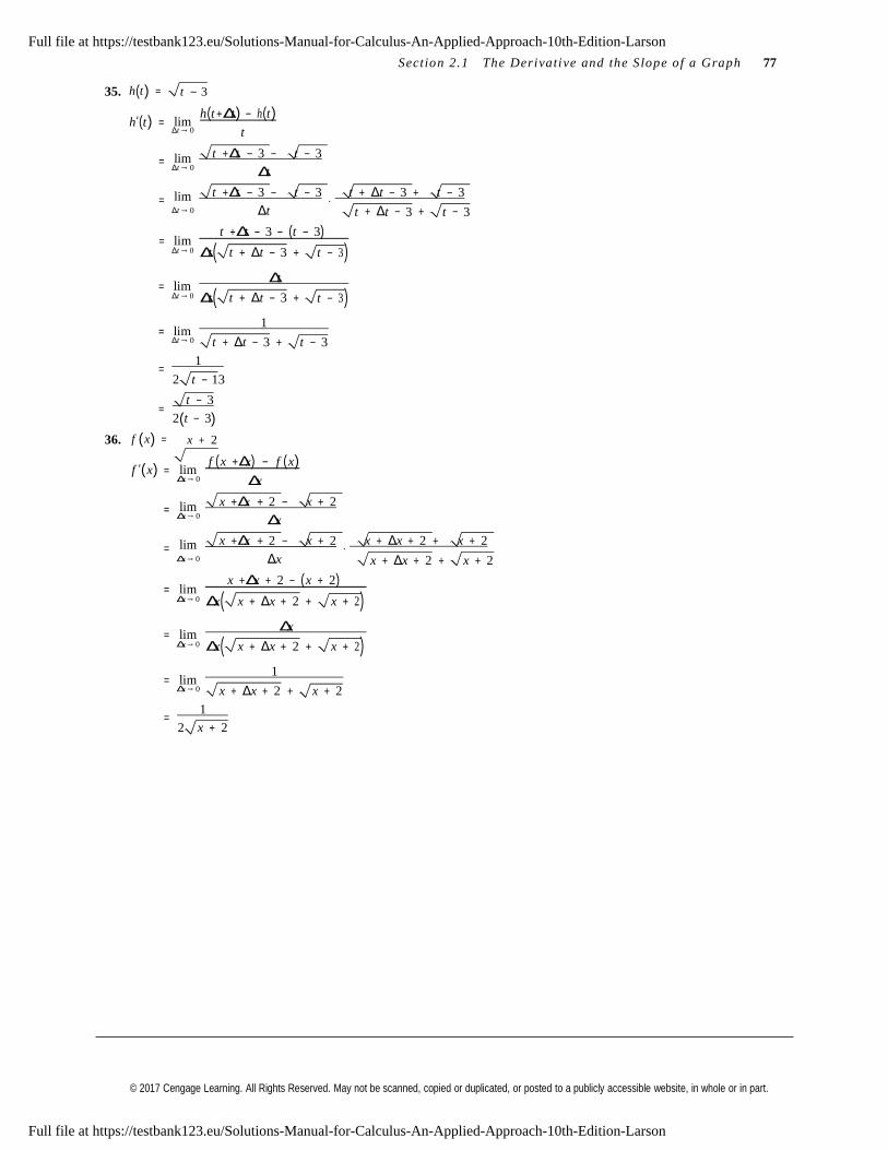
35. h(t ) = t − 3
h′(t ) =
=
=
lim Δt → 0
lim Δt → 0
lim
h(t +Δt ) − h(t ) t
t +Δt − 3 − t − 3
Δt
t +Δt − 3 − t − 3 ⋅
t + Δt − 3 + t − 3
Δt → 0
= lim
Δt t + Δt − 3 +
t +Δt − 3 − (t − 3)
t − 3
Δt → 0 Δt( t + Δt − 3 + t − 3)
= lim Δt
Δt → 0 Δt( t + Δt − 3 + t − 3)
= lim 1
Δt → 0 t + Δt − 3 + t − 3
= 1 2 t − 13
= t − 3 2(t − 3)
36. f (x) = x + 2
f ′(x) =
=
=
lim Δx → 0
lim Δx → 0
lim
f ( x +Δx) − f ( x) Δx
x +Δx + 2 − x + 2
Δx
x +Δx + 2 − x + 2 ⋅
x + Δx + 2 + x + 2
Δx → 0
= lim
Δx x + Δx + 2 +
x +Δx + 2 − ( x + 2)
x + 2
Δx → 0 Δx( x + Δx + 2 + x + 2 )
= lim Δx
Δx → 0 Δx( x + Δx + 2 + x + 2 )
= lim 1
Δx → 0 x + Δx + 2 + x + 2
= 1 2 x + 2
Full file at https://testbank123.eu/Solutions-Manual-for-Calculus-An-Applied-Approach-10th-Edition-Larson
Full file at https://testbank123.eu/Solutions-Manual-for-Calculus-An-Applied-Approach-10th-Edition-Larson
© 2017 Cengage Learning. All Rights Reserved. May not be scanned, copied or duplicated, or posted to a publicly accessible website, in whole or in part.
78 Chapte r 2 Dif ferentiat i on
37. f (t ) = t 3 − 12t
f ′(t ) =
=
=
=
=
=
lim Δt → 0
lim Δt → 0
lim Δt → 0
lim Δt → 0
lim Δt → 0
lim Δt → 0
f (t +Δt ) − f (t ) Δt
(t +Δt )3
− 12(t + Δt ) − (t 3 − 12t ) Δt
t 3 + 3t 2 Δt + 3t (Δt )2
+ (Δt )3
− 12t − 12Δt − t 3 + 12t
Δt
3t 2 Δt + 3t (Δt )2
+ (Δt )3
− 12Δt
Δt
Δt (3t 2 + 3tΔt + (Δt )2
− 12) Δt
(3t 2 + 3tΔt + (Δt)2
− 12)= 3t 2 − 12
38. f (t ) = t 3 + t 2
f ′(t ) =
=
=
=
=
=
lim Δt → 0
lim Δt → 0
lim Δt → 0
lim Δt → 0
lim Δt → 0
lim Δt → 0
f (t +Δt ) − f (t ) Δt
(t +Δt )3
+ (t + Δt )2
− (t 3 + t 2 ) Δt
t 3 + 3t 2 Δt + 3t (Δt )2
+ (Δt )3
+ t 2 + 2tΔt + (Δt )2
− t 3 − t 2
Δt
3t 2 Δt + 3t (Δt )2
+ (Δt )3
+ 2tΔt + (Δt )2
Δt
Δt (3t 2 + 3tΔt + (Δt )2
+ 2t + Δt ) Δt
(3t 2 + 3tΔt + (Δt )2
+ 2t + Δt )
39.
= 3t 2 + 2t
f (x) = 1 x + 2
f ′(x) =
=
=
=
=
lim Δx → 0
lim Δx → 0
lim Δx → 0
lim Δx → 0
lim
f ( x +Δx) − f ( x) Δx
1 −
1 x +Δx + 2 x + 2
Δx
1 ⋅
x + 2 −
1 ⋅
x + Δx + 2 x + Δx + 2 x + 2 x + 2 x + Δx + 2
Δx
x + 2 − (x + Δx + 2) ( x +Δx + 2)( x + 2)
Δx
−Δx
Δx → 0 Δx(x + Δx + 2)(x + 2)
= lim −1
Δx → 0 (x + Δx + 2)(x + 2) 1
= − (x + 2)
2
Full file at https://testbank123.eu/Solutions-Manual-for-Calculus-An-Applied-Approach-10th-Edition-Larson
Full file at https://testbank123.eu/Solutions-Manual-for-Calculus-An-Applied-Approach-10th-Edition-Larson
© 2017 Cengage Learning. All Rights Reserved. May not be scanned, copied or duplicated, or posted to a publicly accessible website, in whole or in part.
2 2
2 2
8
8 8
8 8
4 8
4 8
4 8
− − Δ − (Δ ) +
4
4
Section 2.1 The De rivativ e and the Slo p e of a Grap h 79
40. g (s) = 1
41. ( ) 1 2 ( )
s − 4 f x = 2
x at 2, 2
f ( x +Δx) − f ( x)g′(s) =
lim g(s+Δs) − g (s) f ′(x) = lim
0 Δx
Δs → 0
= lim
Δs → 0
= lim Δs → 0
= lim
Δs
1 −
1 s +Δs − 4 s − 4
Δs
s − 4 − ( s + Δs − 4) (s +Δs − 4)( s − 4)
Δs
s − 4 − ( s + Δs − 4) (s +Δs − 4)( s − 4) 1
⋅
Δx →
= lim
Δx → 0
= lim
Δx → 0
= lim
Δx → 0
= lim Δx → 0
1 ( x + Δx) 2
− 1 x2
Δx
1 ( x2 + 2 xΔx + (Δx)2 ) − 1 x2
Δx
xΔx + (Δx)2
Δx
Δx( x+ Δx) Δx
Δs → 0
= lim
(s + Δs − 4)(s − 4) Δs
−Δs = lim
Δx → 0 (x + Δx)
Δs → 0 Δs(s + Δs − 4)(s − 4) = x
= lim −1 m = f ′(2) = 2
Δs → 0 (s + Δs − 4)(s − 4) y − 2 = 2(x − 2)
= − 1 y = 2x − 2
(s − 4)2
4
(2, 2)
− 6 6
42.
− 4
f (x) = − 1 x2 at (− 4, − 2)
f ′(x) =
=
=
=
=
=
=
lim Δx → 0
lim Δx → 0
lim Δx → 0
lim Δx → 0
lim Δx → 0
lim Δx → 0
lim Δx → 0
f ( x +Δx) − f ( x) Δx
− 1 ( x + Δx)2
− (− 1 x2 ) Δx
− 1 ( x2 + 2 xΔx + (Δx)2 ) + 1 x2
Δx
1 x2 1 x x 1 x 2 1 x2
8 4 8 8
Δx
− 1 xΔx − 1 (Δx)2
Δx
Δx(− 1 x − 1 Δx) Δx
(− 1 x − 1 Δx)= − 1 x
m = f ′(− 4) = − 1 (− 4) = 1
3
−9 9
(−4, −2)
y − (− 2) = 1x − (− 4)y + 2 = x + 4
y = x + 2 −9
Full file at https://testbank123.eu/Solutions-Manual-for-Calculus-An-Applied-Approach-10th-Edition-Larson
Full file at https://testbank123.eu/Solutions-Manual-for-Calculus-An-Applied-Approach-10th-Edition-Larson

© 2017 Cengage Learning. All Rights Reserved. May not be scanned, copied or duplicated, or posted to a publicly accessible website, in whole or in part.
80 Chapte r 2 Dif ferentiat i on
43. f (x) = (x − 1)2
at (− 2, 9)
f ′(x) =
=
=
=
=
=
lim Δx → 0
lim Δx → 0
lim Δx → 0
lim Δx → 0
lim Δx → 0
lim Δx → 0
f ( x +Δx) − f ( x) Δx
( x +Δx − 1)2
− ( x − 1)2
Δx
x 2 + 2 xΔx − 2 x + (Δx)2
− 2Δx + 1 − x 2 + 2 x − 1
Δx
2 xΔx + (Δx)2
− 2Δx
Δx
Δx(2 x + Δx − 2) Δx
(2 x + Δx − 2) 11
= 2 x − 2
m = f ′(−2) = 2(−2) − 2 = −6
(− 2, 9)
y − 9 = −6x − (−2)y = −6 x − 3
− 12 12
− 5
44. f (x) = 2 x2 − 5 at (−1, − 3)
f ′(x) =
=
=
=
=
=
lim Δx → 0
lim Δx → 0
lim Δx → 0
lim Δx → 0
lim Δx → 0
lim Δx → 0
f ( x +Δx) − f ( x) Δx
2( x +Δx)2
− 5 − (2 x2 − 5) Δx
2 x2 + 4 xΔx + 2(Δx)2
− 5 − 2 x2 + 5
Δx
4 xΔx + 2(Δx)2
Δx
Δx(4 x + 2Δx) Δx
(4x + 2Δx)
= 4x
m = f ′(−1) = 4(−1) = − 4
2
−6 6
y − (−3) = − 4(x − (−1))
y + 3 = − 4x − 4
y = − 4x − 7
(−1, −3)
−6
Full file at https://testbank123.eu/Solutions-Manual-for-Calculus-An-Applied-Approach-10th-Edition-Larson
Full file at https://testbank123.eu/Solutions-Manual-for-Calculus-An-Applied-Approach-10th-Edition-Larson
© 2017 Cengage Learning. All Rights Reserved. May not be scanned, copied or duplicated, or posted to a publicly accessible website, in whole or in part.
− 1
Section 2.1 The De rivativ e and the Slo p e of a Grap h 81
45. f (x) = x + 1 at (4, 3)
f ′(x) =
=
=
lim Δx → 0
lim Δx → 0
lim
f ( x +Δx) − f ( x) Δx
x +Δx + 1 − ( x + 1) Δx
x +Δx − x ⋅
x + Δx + x
Δx → 0
= lim
Δx x + Δx + x
x +Δx − x
Δx → 0 Δx( x + Δx + x )
= lim Δx
Δx → 0 Δx( x + Δx + x )
= lim 1
Δx → 0
= 1
x + Δx + x
2 x
m = f ′(4) = 1
= 1 5
2 4 4
y − 3 = 1 (x − 4)
4 − 2
y = 1
x + 2 4
(4, 3)
7
46. f (x) = x + 3 at (6, 3)
f ′(x) =
=
=
lim Δx → 0
lim Δx → 0
lim
f ( x +Δx) − f ( x) Δx
x +Δx + 3 − x + 3
Δx
x +Δx + 3 − x + 3 ⋅
x + Δx + 3 + x + 3
Δx → 0
= lim
Δx x + Δx + 3 +
x +Δx + 3 − ( x + 3) x + 3
Δx → 0 Δx( x + Δx + 3 + x + 3)
= lim Δx
Δx → 0 Δx( x + Δx + 3 + x + 3)
= lim 1
Δx → 0 x + Δx + 3 + x + 3
= 1 2 x + 3
= x + 3 2(x + 3)
m = f ′(6) = 1
= 1
2 6 + 3 6
y − 3 = 1 (x − 6)
6
y − 3 = 1
x − 1 6
y = 1
x + 2 6
7
(6, 3)
−4 8
−1
Full file at https://testbank123.eu/Solutions-Manual-for-Calculus-An-Applied-Approach-10th-Edition-Larson
Full file at https://testbank123.eu/Solutions-Manual-for-Calculus-An-Applied-Approach-10th-Edition-Larson
© 2017 Cengage Learning. All Rights Reserved. May not be scanned, copied or duplicated, or posted to a publicly accessible website, in whole or in part.
(2, −1)
2
5 25
5 (
82 Chapte r 2 Dif ferentiat i on
47.
f (x) = 1
at −
1 , −1
5x
5 f ′(x) =
=
=
=
lim Δx → 0
lim Δx → 0
lim Δx → 0
lim
f ( x +Δx) − f ( x) Δx
1 −
1 5( x +Δx) 5x
Δx
x − (x + Δx) 5 x( x+Δx)
Δx
x − ( x + Δx) ⋅
1
Δx → 0 5x(x + Δx) Δx
= lim −Δx
Δx → 0 5x ⋅ Δx ⋅ (x + Δx)
= lim −1
Δx → 0 5x(x + Δx)
= − 1
5x2
m f 1 1 1
5= ′ −
= − = − = − 5 1
5 −
1 5
y − (−1) = −5 x − − 1
1
5 − 3 3
48.
1 y + 1 = −5 x +
y + 1 = −5x − 1
y = −5x − 2
f (x) = 1
at (2, −1) x − 3
−
1 , − 1
5
− 3
f ′(x) =
=
=
=
=
lim Δ x → 0
lim Δ x → 0
lim Δ x → 0
lim Δ x → 0
lim
f ( x +Δx) − f ( x) Δ x
1 −
1 x +Δx − 3 x − 3
Δ x
1 ⋅
x − 3 −
1 ⋅
x + Δ x − 3 x + Δ x − 3 x − 3 x − 3 x + Δ x − 3
Δ x
x − 3 − (x + Δ x − 3) ( x +Δx − 3)( x − 3)
Δ x
−Δx
Δ x → 0 (x + Δ x − 3)(x − 3)Δ x
= lim −1 = −
1
Δ x → 0 (x + Δ x − 3)(x − 3) (x − 3)2
1 3
m = f ′(2) = −
(2 − 3)2
= −1
y − (−1) = −1(x − 2) y + 1 = − x + 2
y = − x + 1
− 2 7
− 3
Full file at https://testbank123.eu/Solutions-Manual-for-Calculus-An-Applied-Approach-10th-Edition-Larson
Full file at https://testbank123.eu/Solutions-Manual-for-Calculus-An-Applied-Approach-10th-Edition-Larson
© 2017 Cengage Learning. All Rights Reserved. May not be scanned, copied or duplicated, or posted to a publicly accessible website, in whole or in part.
x2
4 4
2 4
2 4
4 2 4 4
x
1
3
3
3 3
3 3
3 3 3
= −
Section 2.1 The De rivativ e and the Slo p e of a Grap h 83
49. f (x) 1 4
50. f (x) = x2 − 7
f ′(x) =
lim Δx → 0
f (x + Δx) −
Δx
f (x) f ′(x) =
lim Δ x → 0
f ( x +Δx) − f ( x) Δ x
= lim Δx → 0
= lim
Δx → 0
= lim
Δx → 0
= lim
Δx → 0
− 1 ( x + Δx)2
− (− 1 x2 ) Δx
− 1 x 2 − 1 xΔx − 1 (Δx)2
+ 1 x2
Δx
− 1 xΔx − 1 (Δx)2
Δx
Δx(− 1 x − 1 Δx) Δx
= lim Δ x → 0
= lim
Δ x → 0
= lim Δ x → 0
= lim Δ x → 0
( x +Δx)2
− 7− ( x2 − 7) Δ x
x2 + 2 xΔ x + (Δ x)2
− 7 − x2 + 7
Δ x
Δ x(2 x + Δ x) Δ x
(2 x + Δ x) = 2x
= lim −
1 x −
1 Δx
Since the slope of the given line is − 2,
Δx → 0 2 4
1 = −
2
Since the slope of the given line is −1,
− 2
x = −1
2x = − 2
x = −1 and f (−1) = − 6.
At the point (−1, − 6), the tangent line parallel to
2x + y = 0 is
x = 2 and f (2) = −1. y − (− 6) = − 2(x − (−1))At the point (2, −1), the tangent line parallel to
x + y = 0 is y − (−1) = −1(x − 2)
y = − x + 1.
y = − 2 x − 8.
51.
f (x) 1
x3= − 3
f ′(x) =
=
=
=
=
=
lim Δ x → 0
lim Δ x → 0
lim Δ x → 0
lim Δ x → 0
lim Δ x → 0
lim Δ x → 0
f ( x +Δx) − f ( x) Δ x
− 1 ( x + Δ x)3
− (− 1 x3 ) Δ x
− 1 ( x3 + 3x 2 Δ x + 3x(Δ x)2
+ (Δ x)3 ) + 1 x3
Δ x
− 1 x3 − x2 Δ x − x(Δ x)2
− 1 (Δ x)3
+ 1 x3
Δ x
Δ x(− x2 − xΔ x − 1 (Δ x)2 )
Δ x
(− x2 − xΔ x − 1 (Δ x)2 ) = − x2
Since the slope of the given line is − 9,
− x2
x2
= −9
= 9
x = ± 3 and f (3) = −9 and f (−3) = 9.
At the point (3, − 9), the tangent line parallel to 9x + y − 6 = 0 is
y − (−9) = −9(x − 3) y = −9x + 18.
At the point (− 3, 9), the tangent line parallel to 9x + y − 6 = 0 is
y − 9 = −9(x − (−3)) y = −9 x − 18.
Full file at https://testbank123.eu/Solutions-Manual-for-Calculus-An-Applied-Approach-10th-Edition-Larson
Full file at https://testbank123.eu/Solutions-Manual-for-Calculus-An-Applied-Approach-10th-Edition-Larson
© 2017 Cengage Learning. All Rights Reserved. May not be scanned, copied or duplicated, or posted to a publicly accessible website, in whole or in part.
2
2
84 Chapte r 2 Dif ferentiat i o n
52. f (x) = x3 + 2
f ′(x) =
=
=
=
=
=
lim Δx → 0
lim Δx → 0
lim Δx → 0
lim Δx → 0
lim Δx → 0
lim Δx → 0
f ( x +Δx) − f ( x) Δx
( x +Δx)3
+ 2 − ( x3 + 2) Δx
x3 + 3x2 Δx + 3x(Δx)2
+ (Δx)3
+ 2 − x3 − 2
Δx
3x2 Δx + 3(Δx)2
+ (Δx)3
Δx
Δx(3x2 + 3xΔx + (Δx)2 )
Δx
(3x2 + 3xΔx + (Δx)2 )
= 3x2
The slope of the given line is
3x − y − 4 = 0
y = 3x − 4
m = 3.
3x2 = 3
x2 = 1
x = ±1
x = 1 and f (1) = 3
x = −1 and f (−1) = 1
At the point (1, 3), the tangent line parallel to 3x − y − 4 = 0 is
y − 3 = 3(x − 1)
y − 3 = 3x − 3
y = 3x.
At the point (−1, 1), the tangent line parallel to 3x − y − 4 = 0 is
y − 1 = 3(x − (−1))
y − 1 = 3(x + 1)
y − 1 = 3x + 3
y = 3x + 4.
53. y is differentiable for all x ≠ −3.
At (−3, 0), the graph has a node.
54. y is differentiable for all x ≠ ± 3.
At (± 3, 0), the graph has a cusp.
55. y is differentiable for all x ≠ − 1 .
At (− 1 , 0), the graph has a vertical tangent line.
56. y is differentiable for all x > 1.
The derivative does not exist at endpoints.
57. y is differentiable for all x ≠ ± 2.
The function is not defined at x = ± 2.
58. y is differentiable for all x ≠ 0.
The function is discontinuous at x = 0.
Full file at https://testbank123.eu/Solutions-Manual-for-Calculus-An-Applied-Approach-10th-Edition-Larson
Full file at https://testbank123.eu/Solutions-Manual-for-Calculus-An-Applied-Approach-10th-Edition-Larson
© 2017 Cengage Learning. All Rights Reserved. May not be scanned, copied or duplicated, or posted to a publicly accessible website, in whole or in part.
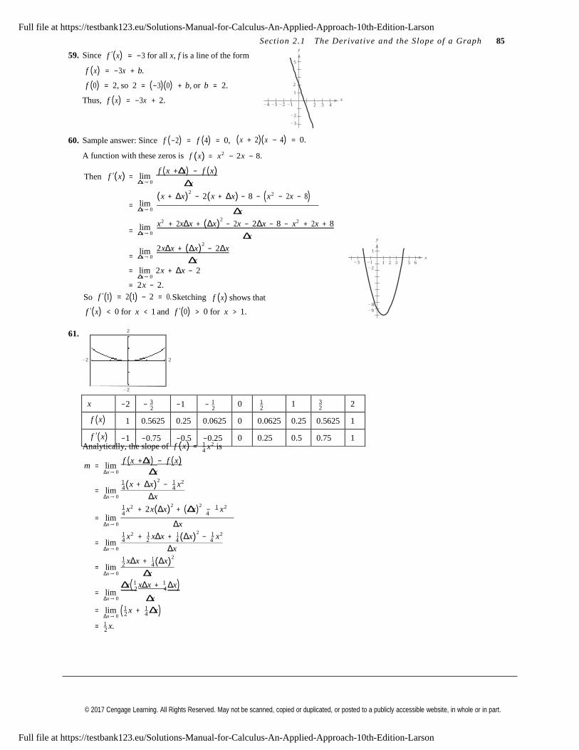
x −2 − 3 −1 − 1 0 1 2
1 3 2
2
f (x) 1 0.5625 0.25 0.0625 0 0.0625 0.25 0.5625 1
f ′(x) −1 −0.75 −0.5 −0.25 0 0.25 0.5 0.75 1
4
2 4
2
Section 2.1 The De rivativ e and the Slo p e of a Grap h 85
59. Since y
f ′(x) = −3 for all x, f is a line of the form 5
f (x) = −3x + b.
f (0) = 2, so 2 = (−3)(0) + b, or b = 2. 2
1
Thus, f (x) = −3x + 2. − 4 − 3 − 2 − 1
x
2 3 4
60. Sample answer: Since
f (−2) =
f (4) = 0,
− 2
− 3
(x + 2)(x − 4) = 0.
A function with these zeros is f (x) = x2 − 2 x − 8.
Then
f ′(x) =
=
=
=
lim Δx → 0
lim Δx → 0
lim Δx → 0
lim Δx → 0
f ( x +Δx) − f ( x) Δx
(x + Δx)2
− 2(x + Δx) − 8 − (x2 − 2 x − 8) Δx
x2 + 2 xΔx + (Δx)2
− 2 x − 2Δx − 8 − x2 + 2 x + 8
Δx
2 xΔx + (Δx)2
− 2Δx
Δx
y
1
− 3 −1
x 1 2 3 5 6
= lim 2x + Δx − 2 − 2
Δx → 0
= 2x − 2.
So f ′(1) = 2(1) − 2 = 0. Sketching
f (x) shows that − 8
f ′(x) < 0 for x < 1 and f ′(0) > 0 for x > 1. − 9
61. 2
− 2 2
− 2
2 2
Analytically, the slope of f (x) = 1 x2 is
f ( x +Δx) − f ( x) m = lim
Δx → 0 Δx 1 (x + Δx)
2 − 1 x2
= lim 4 4
Δx → 0 Δx 1 x2 + 2x(Δx)
2 + (Δx)
2 − 1 x2
= lim 4 4
Δx → 0 Δx 1 x2 + 1 xΔx + 1 (Δx)
2 − 1 x2
= lim 4 2 4 4
Δx → 0 Δx 1 xΔx + 1 (Δx)
2
= lim 2 4
Δx → 0
= lim
Δx → 0
Δx
Δx( 1 xΔx + 1 Δx) Δx
= lim (1 x + 1 Δx) Δx → 0 2 4
= 1 x.
Full file at https://testbank123.eu/Solutions-Manual-for-Calculus-An-Applied-Approach-10th-Edition-Larson
Full file at https://testbank123.eu/Solutions-Manual-for-Calculus-An-Applied-Approach-10th-Edition-Larson
© 2017 Cengage Learning. All Rights Reserved. May not be scanned, copied or duplicated, or posted to a publicly accessible website, in whole or in part.
x − 2 − 3 −1 − 1 0 1 2
1 3 2
2
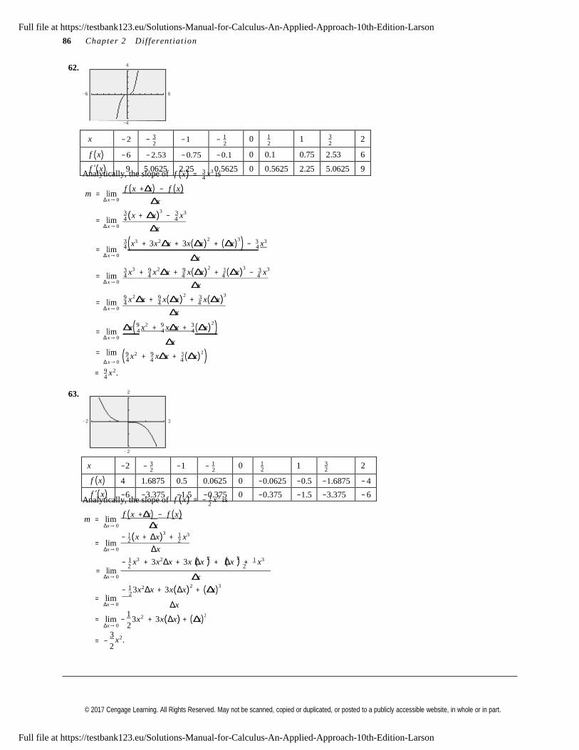
f (x) − 6 − 2.53 − 0.75 − 0.1 0 0.1 0.75 2.53 6
f ′(x) 9 5.0625 2.25 0.5625 0 0.5625 2.25 5.0625 9
x −2 − 3 −1 − 1 0 1 2
1 3 2
2
f (x) 4 1.6875 0.5 0.0625 0 −0.0625 −0.5 −1.6875 − 4
f ′(x) −6 −3.375 −1.5 −0.375 0 −0.375 −1.5 −3.375 − 6
4
4 4
4 4 4
4 4
4 4 4
4 4 4 4 4
2
( ) ( )
= −
86 Chapte r 2 Dif ferentiat i on
62. 4
−6 6
−4
2 2
Analytically, the slope of f ( x) = 3 x3 is
m = lim Δ x → 0
= lim
Δ x → 0
= lim
Δ x → 0
= lim
Δ x → 0
= lim
Δ x → 0
= lim
Δ x → 0
= lim
f ( x +Δx) − f ( x) Δ x
3 (x + Δ x)3
− 3 x3
Δ x
3 ( x3 + 3x 2 Δ x + 3x(Δ x)2
+ (Δ x)3 ) − 3 x3
Δ x
3 x3 + 9 x2Δ x + 9 x(Δ x)2
+ 3 (Δ x)3
− 3 x3
Δ x
9 x2Δ x + 9 x(Δ x)2
+ 3 x(Δ x)3
Δ x
Δ x( 9 x 2 + 9 xΔ x + 3 (Δ x)2 )
Δ x
(9 x2 + 9 xΔ x + 3 (Δ x)2 )
Δ x → 0 4 4 4
9 2
= 4
x .
63. 2
− 2 2
− 2
2 2
Analytically, the slope of f (x) = − 1 x3 is
f ( x +Δx) − f ( x) m = lim
Δx → 0 Δx
− 1 (x + Δx)3
+ 1 x3
= lim 2 2
Δx → 0
= lim
Δx → 0
Δx
− 1 x3 + 3x2Δx + 3x Δx 2
+ Δx 3 + 1 x3
2 2
Δx
− 1 3x2Δx + 3x(Δx)2
+ (Δx)3
= lim 2
Δx → 0 Δx
= lim − 1
3x2 + 3x(Δx) + (Δx)2
Δx → 0
3 x2 .
2
2
Full file at https://testbank123.eu/Solutions-Manual-for-Calculus-An-Applied-Approach-10th-Edition-Larson
Full file at https://testbank123.eu/Solutions-Manual-for-Calculus-An-Applied-Approach-10th-Edition-Larson
© 2017 Cengage Learning. All Rights Reserved. May not be scanned, copied or duplicated, or posted to a publicly accessible website, in whole or in part.
x −2 − 3 −1 − 1 0 1 2
1 3 2
2
f (x) −6 −3.375 −1.5 −0.375 0 −0.375 −1.5 −3.375 −6
f ′(x) 6 4.5 3 1.5 0 −1.5 −3 −4.5 −6
2
2 2
− 4
Section 2.1 The De rivativ e and the Slo p e of a Grap h 87
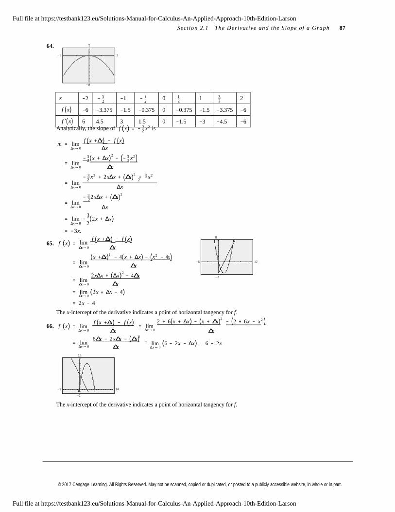
64. 2
− 2 2
− 8
2 2
Analytically, the slope of f (x) = − 3 x2 is
f ( x +Δx) − f ( x) m = lim
Δx → 0
= lim
Δx → 0
Δx
− 3 ( x + Δx)2
− (− 3 x2 ) Δx
− 3 x2 + 2xΔx + (Δx)2 + 3 x2
= lim 2 2
Δx → 0 Δx
− 3 2xΔx + (Δx)2
= lim 2
Δx → 0 Δx
= lim − 3 (2x + Δx)
Δx → 0 2
= −3x.
65.
f ′(x) = f ( x +Δx) − f ( x) 8
limΔx → 0
= lim
Δx → 0
= lim
Δx → 0
Δx
( x +Δx)2
− 4( x + Δx) − ( x2 − 4 x) − 6 12
Δx
2 xΔx + (Δx)2
− 4Δx
Δx
= lim (2x + Δx − 4) Δx → 0
= 2x − 4
The x-intercept of the derivative indicates a point of horizontal tangency for f.
66.
f ′(x) =
lim Δx → 0
f ( x +Δx) − f ( x) Δx
= lim
Δx → 0
2
2 + 6( x + Δx) − ( x + Δx) 2
− (2 + 6 x − x 2 ) Δx
= lim Δx → 0
6Δx − 2 xΔx − (Δx) =
Δx lim (6 − 2 x − Δx) = 6 − 2 x Δx → 0
13
−7 14
−1
The x-intercept of the derivative indicates a point of horizontal tangency for f.
Full file at https://testbank123.eu/Solutions-Manual-for-Calculus-An-Applied-Approach-10th-Edition-Larson
Full file at https://testbank123.eu/Solutions-Manual-for-Calculus-An-Applied-Approach-10th-Edition-Larson
© 2017 Cengage Learning. All Rights Reserved. May not be scanned, copied or duplicated, or posted to a publicly accessible website, in whole or in part.
( )
( )
88 Chapte r 2 Dif ferentiat i on
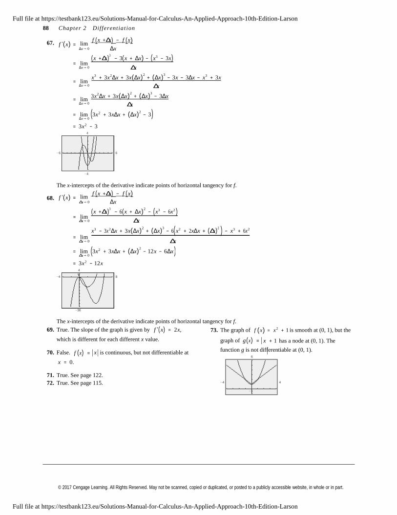
67.
f ′(x) = f ( x +Δx) − f ( x) limΔx → 0
= lim
Δx → 0
= lim
Δx → 0
= lim
Δx → 0
Δx
( x +Δx)3
− 3( x + Δx) − ( x3 − 3x) Δx
x3 + 3x 2 Δx + 3x(Δx)2
+ (Δx)3
− 3x − 3Δx − x3 + 3x
Δx
3x 2 Δx + 3x(Δx)2
+ (Δx)3
− 3Δx
Δx
= lim 3x2 + 3xΔx + (Δx)2
− 3 Δx → 0
= 3x2 − 3 4
− 6 6
− 4
The x-intercepts of the derivative indicate points of horizontal tangency for f.
68.
f ′(x) = f ( x +Δx) − f ( x) limΔx → 0
= lim
Δx → 0
= lim
Δx → 0
Δx
( x +Δx)3
− 6( x + Δx)2
− ( x3 − 6 x2 ) Δx
x3 − 3x2 Δx + 3x(Δx)2
+ (Δx)3
− 6( x2 + 2 xΔx + (Δx)2 ) − x3 + 6 x2
Δx
= lim 3x2 + 3xΔx + (Δx)2
− 12x − 6Δx Δx → 0
= 3x2 − 12x 4
−4 8
−36
The x-intercepts of the derivative indicate points of horizontal tangency for f.
69. True. The slope of the graph is given by f ′(x) = 2x, 73. The graph of f (x) = x2 + 1 is smooth at (0, 1), but the
which is different for each different x value. graph of g (x) = x + 1 has a node at (0, 1). The
70. False.
x = 0.
f (x) =
x is continuous, but not differentiable at function g is not differentiable at (0, 1). 6
71. True. See page 122.
72. True. See page 115. − 4 4
− 1
Full file at https://testbank123.eu/Solutions-Manual-for-Calculus-An-Applied-Approach-10th-Edition-Larson
Full file at https://testbank123.eu/Solutions-Manual-for-Calculus-An-Applied-Approach-10th-Edition-Larson
© 2017 Cengage Learning. All Rights Reserved. May not be scanned, copied or duplicated, or posted to a publicly accessible website, in whole or in part.
4
4
3
−3
2
Section 2.2 Som e Rule s for D i f fe r e nt ia t i on 89
Section 2.2 Some Rules for Differentiation
Skills Warm Up
1. (a) 2 x2 , x = 2
2(22 ) = 2(4) = 8
1 5. x
−3 4 = 1
4x3 4
(b) (5x)2 , x = 2
6. 1(3)x2 1
− 2 x −1 2 + 1
x −2 3 = x2 − x−1 2 + 1
x −2 3
5(2)
2
= 102
= 100
3 2 3 3
= x2 − 1
+ 1
(c)
6x−2 , x = 2
7. 3x2 + 2 x = 0
x 3 3 x2
6(2)−2
= 6(1 ) = 3 x(3x + 2) = 0
x = 02. (a)
1 , x = 2
(3x)2
3x + 2 = 0 → x = − 2
1 1 1
8. x3 − x = 02
= 2
=3(2)
1
6 36 x(x2 − 1) = 0
x(x + 1)(x − 1) = 0(b) , x = 2 4x3
1 =
1 =
1
x = 0
x + 1 = 0 → x = −14(23 ) 4(8) 32
x 1 0 x 1
(c) (2 x)
, x = 2
9. x2
− = → =
+ 8x − 20 = 0
4 x−2
−3
−3 2
(x + 10)(x − 2) = 0
2(2) = 4
= 2
= 1
x + 10 = 0 → x = −10
4(2)−2
4(2)−2
4(43 ) 64 10.
x − 2 = 0 → x = 2
3x2 − 10x + 8 = 0
3. 4(3)x3 + 2(2)x = 12x3 + 4x = 4x(3x2 + 1) ( )( )3x − 4 x − 2 = 0
4
4. 1 ( ) 2
3 1 2
3 2 3 3
1 2 ( 3 2 ) 3x − 4 = 0 → x =
32
3 x − 2
x = 2
x − 2
x = 2
x x − 1
x − 2 = 0 → x = 2
1. y = 3
y′ = 0
2. f (x) = − 8
6. h(x) = 6 x5
h′(x) = 30x4
5x4
f ′(x) = 0
3. y = x5
7. y =
y′ =
3
20 x3
= 10
x3
y′ = 5x4
4. f (x) = 1
= x−6
x6
6 3
3t 2
8. g (t ) = 4
3
f ′(x) = − 6 x−7
6 = −
x7
g′(t ) = t 2
5. h(x) = 3x3
h′(x) = 9x2
9. f (x) = 4x
f ′( x) = 4
Full file at https://testbank123.eu/Solutions-Manual-for-Calculus-An-Applied-Approach-10th-Edition-Larson
Full file at https://testbank123.eu/Solutions-Manual-for-Calculus-An-Applied-Approach-10th-Edition-Larson
© 2017 Cengage Learning. All Rights Reserved. May not be scanned, copied or duplicated, or posted to a publicly accessible website, in whole or in part.
3 3
( )
x
= −
= −
2
4 2
90 Chapte r 2 Dif ferentiat i on
10. g (x) = x =
1 x 17. s(t) = 4t 4 − 2t + t + 3
11.
3 3
g′(x) = 1 3
y = 8 − x3
y = − 3x2
18.
19.
s′(t ) = 16t 2 − 4t + 1
y = 2x3 − x2 + 3x − 1
y′ = 6x2 − 2x + 3
g (x) = x2 3
12. y = t 2 − 6
y′ = 2t
g′(x) = 2
x−1 3 = 2
3 3x1 3
13.
f (x) = 4x2 − 3x
20. h(x) = x5 2
f ′(x) = 8x − 3 h′(x) = 5 x3 2 2
14. g (x) = 3x2 + 5x3
g′(x) = 6x + 15x2
= 15x2 + 6x
21. y = 4t 4 3
y′ = 4( 4 )t1 3 = 16 t1 3
15. f (t ) = − 3t 2 + 2t − 4
f ′(t ) = − 6t + 2
22. f (x) = 10x1 6
f ′(x) = 5
x−5 6 = 5
= 5
16.
y = 7 x3 − 9x2 + 8
y′ = 21x2 − 18x
23.
y = 4x
3 3x5 6
− 2 + 2x2
3 6 x5
y′ = −8x−3 + 4x1 = − 8
+ 4x x3
24. s(t ) = 8t − 4 + t
s′(t ) = 8 − 4t − 6 + 1 = − 32
+ 1 t 6
Function Rewrite Differentiate Simplify
25. y = 2 7 x4
y = 2
x− 4
7
y′ = − 8
x−5
7
8 y′ = −
7 x5
26.
y = 2 3x2
y = 2
x−2
3
4 y′ = − −3
3
4 y′ = −
3x3
27.
28.
y = 1
(4 x)3
y = π
(2 x)6
y = 1
x−3
64
y = π
x−6
64
y′ 3
x−4
64
y′ 6π
x−7
64
y′ = − 3
64x4
y′ = − 3π
32x7
29. y = 4
(2 x)−5
4 x
y = 128x5
4
y′ = 128(5)x4
3
y′ = 640 x4
3
30. y = x−3
y = 4x y′ = 4(4)x y′ = 16x
31.
y = 6 x
y = 6 x1 2
y′ = 6(1 )x−1 2
y′ = 3
x
32.
y = 3 x
y = 3
x1 2
y′ = 3 1
x−1 2
y′ = 3
4 4 8 x
Full file at https://testbank123.eu/Solutions-Manual-for-Calculus-An-Applied-Approach-10th-Edition-Larson
Full file at https://testbank123.eu/Solutions-Manual-for-Calculus-An-Applied-Approach-10th-Edition-Larson
© 2017 Cengage Learning. All Rights Reserved. May not be scanned, copied or duplicated, or posted to a publicly accessible website, in whole or in part.
2 2 2
4
2
= −
Section 2.2 Som e Rule s for D iffe r e ntiat i on 91
Function Rewrite Differentiate Simplify
33.
y = 1
y = 1
x−1 6
y′ =
1 −
1 x− 7 6
y′ = − 1
7 6 x 7
7
6 6 7 42 x
34.
y = 3
y = 3
x−3 4
y′ = 3
− 3
x− 7 4
y′ = − 9
2 4
x3 2
2
4 4 7 8 x
35.
y = 5 8x
y = (8x)1 5
= 81 5 x1 5 y′ = 81 5 1
x− 4 5 1 5 8 5 8
y′ = 81 5 = = 5
5x4 5 5 4 5x 5 x
36.
y = 3 6x2
y = 3 6 (x)2 3
y′ = 3 6 2
x−1 3 3
y′ = 2 3 6 3
3 x
37. y = x3 2 43. f (x) = − 1 x(1 + x2 ) = − 1 x − 1 x3
y′ = 3 x1 2
1 3 2
2 f ′(x) = − 2
− 2
x
At the point (1, 1), y′ = 3 (1)1 2
= 3 = m. f ′(1) = − 1 − 3 = −22 2 2 2
38. y = x−1
y′ = x− 2
1 = −
44. f (x) = 3(5 − x)2
f ′(x) = −30 + 6 x
= 75 − 30x + 3x2
x2
3 4
1 16
f ′(5) = −30 + (6)(5) = 0
At the point , , y′ = − 2
= − = m. 4 3 ( 3 ) 9 45. (a) y = −2x4 + 5x2 − 3
y′ = −8x3 + 10 x
39. f (t) = t − 4
m y′(1)
8 10 2
f ′(t) = − 4t −5 4 t 5
At the point
= = − + =
The equation of the tangent line is
y − 0 = 2(x − 1)
y = 2x − 2. 1 , 16, f
1 = −
4 4 = −128 = m.
′ = − 2 2 1
5
1
32 (b) and (c) 3.1
40. f (x) = x−1 3
− 4.7 4.7
f ′(x) 1
x− 4 3 = − 1
= − 3 3x4 3
− 3.1
1 ′
1 1 46. (a)
y = x3 + x + 4At the point 8, 2
, f (8) = − = − = m. 4 3 48 3(8)
y′ = 3x2 + 1
41. f (x) = 2x3 + 8x2 − x − 4 m = y′(− 2) = 3(− 2)2
+ 1 = 13
42.
f ′(x) = 6x2 + 16 x − 1
At the point
(−1, 3), f ′(−1) = 6(−1)2
+ 16(−1) − 1 = −11 = m.
f (x) = x4 − 2 x3 + 5x2 − 7 x
The equation of the tangent line is
y − (−6) = 13x − (− 2)
y + 6 = 13x + 26
y = 13x + 20.
f ′(x) = 4x3 − 6x2 + 10x − 7
At the point
(−1, 15), f ′(−1) = 4(−1)3
− 6(−1)2
+ 10(−1) − 7
= − 4 − 6 − 10 − 7 = − 27 = m.
(b) and (c)
− 5
50
5
− 50
Full file at https://testbank123.eu/Solutions-Manual-for-Calculus-An-Applied-Approach-10th-Edition-Larson
Full file at https://testbank123.eu/Solutions-Manual-for-Calculus-An-Applied-Approach-10th-Edition-Larson
© 2017 Cengage Learning. All Rights Reserved. May not be scanned, copied or duplicated, or posted to a publicly accessible website, in whole or in part.
3
92 Chapte r 2 Dif ferentiat i on
47. (a) f (x) = 3 x + 5 x = x1 3 + x1 5 50. (a) y = (2 x + 1)
2
f ′(x) = 1
x−2 3 + 1
x−4 5 = 1
+ 1 y = 4 x2 + 4 x + 1
3 5 3x2 3 5x4 5
y′ = 8x + 4
m = f ′(1) = 1
+ 1
= 8
3 5 15 m = y′ = 8(0) + 4 = 4
The equation of the tangent line is
y − 2 = 8
(x − 1) 15
The equation of the tangent line is
y − 1 = 4(x − 0)
y = 4x + 1.
y = 8
x + 22
. 15 15
(b) and (c)
3.1
(b) and (c) 3
− 4 2
− 4.7 4.7
− 1
− 3.1 51. f (x) = x2 − 4 x−1 − 3x−2
f ′ x
= 2x + 4 x−2 + 6 x−3
= 2x + 4
+ 6
48. (a) f (x) = 1
− x = x−2 3 − x 3 x2
( ) x2 x3
f ′(x) 2
x−5 3 − 1 52. f (x) = 6x2 − 5x−2 + 7 x−3
= − 3 10 21
m = f ′(−1) = 2 1
− 1 = − ( )
x x4
f ′ x
3 3
= 12x + 10x−3 − 21x− 4 = 12 x +
3 −
The equation of the tangent line is
y − 2 = − 1 (x + 1)
53. f (x) = x2 − 2x − 2
= x2 − 2x − 2 x−4
x4
8
y = − 1 x + 5. ′( )
2 2 8 −5 2 2
x3 3
(b) and (c) 4 f x = x − + x = x − +
5
1
54. f (x) = x2 + 4x + = x2 + 4x + x−1
x
− 5 4
− 2
55.
f ′(x) = 2 x + 4 − x−2
f (x) = x4 5 + x
= 2x + 4 − 1 x2
f ′ x
= 4
x−1 5 + 1 = 4
+ 1
49. (a)
y = 3x x2 −
2 ( ) 5 5x1 5
x
y = 3x3 − 6
56.
f (x) = x1 3 − 1
y′ = 9x2
f ′(x) 1
x−2 3 1
m = y′ = 9(2)2
= 36
= = 3 3x2 3
The equation of the tangent line is
y − 18 = 36(x − 2)
y = 36x − 54.
57. 58.
f (x) = x(x2 + 1) = x3 + x
f ′(x) = 3x2 + 1
f (x) = (x2 + 2 x)(x + 1) = x3 + 3x2 + 2 x
(b) and (c) 50
f ′(x) = 3x2 + 6 x + 2
− 5 5
− 50
Full file at https://testbank123.eu/Solutions-Manual-for-Calculus-An-Applied-Approach-10th-Edition-Larson
Full file at https://testbank123.eu/Solutions-Manual-for-Calculus-An-Applied-Approach-10th-Edition-Larson
© 2017 Cengage Learning. All Rights Reserved. May not be scanned, copied or duplicated, or posted to a publicly accessible website, in whole or in part.
3
2
Section 2.2 Som e Rule s for D i f fe rentia t i on 93
59.
2x3 − 4x2 + 3 f (x) = = 2x − 4 + 3x−2
x2
f ′(x) = 2 − 6x−3 = 2 − 6
=
2 x − 6 = 2( x 3 − 3)
x3 x3 x3
60. 2x2 − 3x + 1
f (x) = = 2x − 3 + x−1
x
f ′(x) = 2 − x−2 1 2x2 − 1 = 2 − =
x2 x2
61. 4 x3 − 3x2 + 2x + 5
f (x) = = 4x − 3 + 2x−1 + 5x−2
x2
2 10 4x3 − 2 x − 10 f ′(x) = 4 − 2 x−2 − 10 x−3 = 4 − − =
x2 x3 x3
62.
63.
−6 x3 + 3x2 − 2 x + 1 f (x) = = −6x2 + 3x − 2 + x−1
x
f ′(x) = −12x + 3 − x−2 = −12x + 3 − 1 x2
y = x4 − 2 x + 3
y′ = 4x3 − 4 x = 4x(x2 − 1) = 0 when x = 0, ±1
If x = ±1, then y = (± 1)4
− 2(± 1)2
+ 3 = 2.
The function has horizontal tangent lines at the points
(0, 3), (1, 2), and (−1, 2).
67.
68.
y = x2 + 3
y′ = 2x
Set y′ = 4.
2x = 4
x = 2
If x = 2, y = (2)2
+ 3 = 7 → (2, 7).
The graph of y = x2 + 3 has a tangent line with slope
m = 4 at the point (2, 7).
y = x2 + 2 x
64.
y = x3 + 3x2
y′ = 2x + 2
y′ = 3x2 + 6 x = 3x(x + 2) = 0 when x = 0, − 2.
The function has horizontal tangent lines at the points
(0, 0) and (−2, 4).
Set y′ = 10.
2x + 2 = 10
x = 4
x = 4, y =
4 2
+ 2 4
= 24 →
4, 24 .
65. y = 1 x2 + 5x If ( ) ( ) ( )
2
y′ = x + 5 = 0 when x = −5. The graph of y = x + 2 x has a tangent line with slope
The function has a horizontal tangent line at the point m = 10 at the point (4, 24).
( 25 )
−5, − 2
.
66. y = x2 + 2 x
y′ = 2x + 2 = 0 when x = −1.
The function has a horizontal tangent line at the point
(−1, −1).
Full file at https://testbank123.eu/Solutions-Manual-for-Calculus-An-Applied-Approach-10th-Edition-Larson
Full file at https://testbank123.eu/Solutions-Manual-for-Calculus-An-Applied-Approach-10th-Edition-Larson
© 2017 Cengage Learning. All Rights Reserved. May not be scanned, copied or duplicated, or posted to a publicly accessible website, in whole or in part.
94 Chapte r 2 Dif ferentiat i on
69. (a) y
4
2
70. (a) y
5 g f
4
g f
x
− 4 − 2 2 4
− 2
− 4
3
2
− 3 − 2 − 1
− 1
x 1 2 3
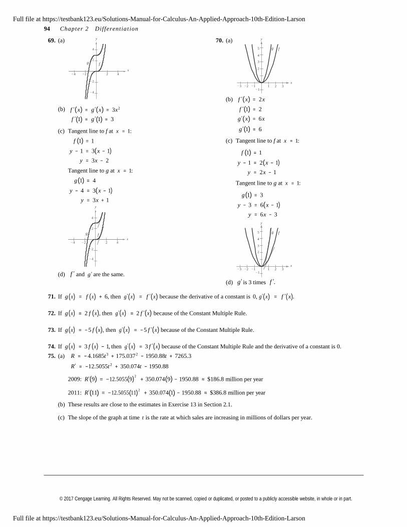
(b)
f ′(x) = g′(x) = 3x2
f ′(1) = g′(1) = 3
(b) f ′(x) = 2 x
f ′(1) = 2
g′(x) = 6 x
(c) Tangent line to f at x = 1:
f (1) = 1
y − 1 = 3(x − 1)
y = 3x − 2
Tangent line to g at x = 1:
g (1) = 4
y − 4 = 3(x − 1)
y = 3x + 1 y
4
2
g f
x
g′(1) = 6
(c) Tangent line to f at x = 1:
f (1) = 1
y − 1 = 2(x − 1)
y = 2 x − 1
Tangent line to g at x = 1:
g (1) = 3
y − 3 = 6(x − 1)
y = 6 x − 3
y
5 g f
4− 4 − 2 2 4
3 − 2
2
− 4
(d) f ′ and g ′ are the same.
− 3 − 2 − 1
− 1
x
1 2 3
(d) g′ is 3 times f ′.
71. If g (x) = f (x) + 6, then g′(x) = f ′(x) because the derivative of a constant is 0, g′(x) = f ′(x).
72. If g (x) = 2 f (x), then g′(x) = 2 f ′(x) because of the Constant Multiple Rule.
73. If g (x) = − 5 f (x), then g′(x) = − 5 f ′(x) because of the Constant Multiple Rule.
74. If g (x) = 3 f (x) − 1, then g′(x) = 3 f ′(x) because of the Constant Multiple Rule and the derivative of a constant is 0.
75. (a) R = − 4.1685t 3 + 175.0372 − 1950.88t + 7265.3
R′ = −12.5055t 2 + 350.074t − 1950.88
2009: R′(9) = −12.5055(9)2
+ 350.074(9) − 1950.88 ≈ $186.8 million per year
2011: R′(11) = −12.5055(11)2
+ 350.074(1) − 1950.88 ≈ $386.8 million per year
(b) These results are close to the estimates in Exercise 13 in Section 2.1.
(c) The slope of the graph at time t is the rate at which sales are increasing in millions of dollars per year.
Full file at https://testbank123.eu/Solutions-Manual-for-Calculus-An-Applied-Approach-10th-Edition-Larson
Full file at https://testbank123.eu/Solutions-Manual-for-Calculus-An-Applied-Approach-10th-Edition-Larson
© 2017 Cengage Learning. All Rights Reserved. May not be scanned, copied or duplicated, or posted to a publicly accessible website, in whole or in part.
Section 2.2 Som e Rule s for D i f fe rentia t i on 95
76. (a) R = − 2.67538t 4 + 94.0568t 3 − 1155.203t 2 + 6002.42t − 9794.2
R′ = −10.70152t 3 + 282.1704t 2 − 2310.406t + 6002.42
2010: R′(10) = −10.70152(10)3
+ 282.1704(10)2
− 2310.406(10) + 6002 ≈ $413.88 million per year
2012: R′(12) = −10.70152(12)3
+ 282.1704(12)2
− 2310.406(12) + 6002 ≈ $417.86 million per year
(b) These results are close to the estimates in Exercise 14 in Section 2.1.
(c) The slope of the graph at time t is the rate at which sales are increasing in millions of dollars per year.
77. (a) More men and women seem to suffer from migraines
between 30 and 40 years old. More females than
males suffer from migraines. Fewer people whose
income is greater than or equal to $30,000 suffer
from migraines than people whose income is less
than $10,000.
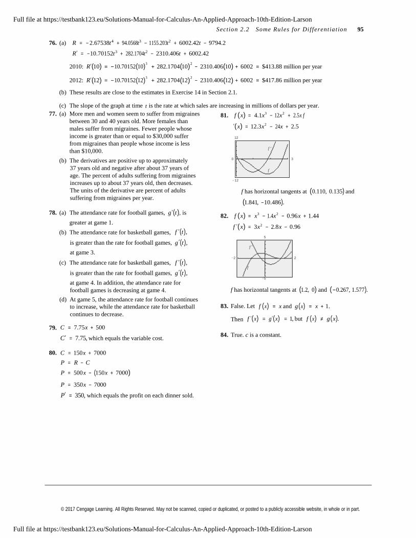
81. f (x) = 4.1x3 − 12 x2 + 2.5x f
′(x) = 12.3x2 − 24 x + 2.5 12
f ′
(b) The derivatives are positive up to approximately
37 years old and negative after about 37 years of
age. The percent of adults suffering from migraines
increases up to about 37 years old, then decreases.
0 3
f
− 12
The units of the derivative are percent of adults
suffering from migraines per year.
78. (a) The attendance rate for football games, g′(t ), is
greater at game 1.
82.
f has horizontal tangents at (0.110, 0.135) and
(1.841, −10.486).
f (x) = x3 − 1.4 x2 − 0.96x + 1.44
f ′(x) = 3x2 − 2.8x − 0.96(b) The attendance rate for basketball games, f ′(t ),
5
is greater than the rate for football games, g′(t ), at game 3.
f ′
−2 2
(c) The attendance rate for basketball games, f ′(t ), f
is greater than the rate for football games, g′(t ), at game 4. In addition, the attendance rate for
football games is decreasing at game 4.
(d) At game 5, the attendance rate for football continues
−5
f has horizontal tangents at (1.2, 0) and (−0.267, 1.577).
to increase, while the attendance rate for basketball
continues to decrease.
83. False. Let f (x) = x and g (x) = x + 1.
79.
C = 7.75x + 500
Then f ′(x) = g′(x) = 1, but f (x) ≠ g (x).
C′ = 7.75, which equals the variable cost. 84. True. c is a constant.
80. C = 150 x + 7000
P = R − C
P = 500 x − (150 x + 7000)
P = 350x − 7000
P′ = 350, which equals the profit on each dinner sold.
Full file at https://testbank123.eu/Solutions-Manual-for-Calculus-An-Applied-Approach-10th-Edition-Larson
Full file at https://testbank123.eu/Solutions-Manual-for-Calculus-An-Applied-Approach-10th-Edition-Larson
© 2017 Cengage Learning. All Rights Reserved. May not be scanned, copied or duplicated, or posted to a publicly accessible website, in whole or in part.
10
10
5 5 2
9
96 Chapte r 2 Dif ferentiat i on
Section 2.3 Rates of Change: Velocity and Marginals
Skills Warm Up
−63 − (−105) 42
8. y = −16 x2 + 54x + 70
1. = 21 − 7 14
= 3
y′ = −32 x + 54
9. A = 1 (−2r 3 + 3r 2 + 5r )2.
−43 − 35 =
6 − (− 7)
− 78
13
A′ = 1 (−6r 2 + 6r + 5)= − 6 A′ = − 3 r 2 + 3 r + 1
3. 24 − 33
= − 9
= − 3
10. y = 1 (6x3 − 18x2 + 63x − 15)9 − 6 3 9
y′ = 1 (18x2 − 36x + 63)4.
40 − 16 = 24 12
= y′ = 2 x2 − 4 x + 718 − 8 10 5
5. y = 4x2 − 2x + 7
y′ = 8x − 2
6. s = − 2t 3 + 8t 2 − 7t
s′ = − 6t 2 + 16t − 7
7. s = −16t 2 + 24t + 30
s′ = −32t + 24
11.
12.
x 2
y = 12 x − 5000
y′ = 12 − 2 x
5000
y′ = 12 − x 2500
y = 138 + 74x −
3x2
x3
10,000
y′ = 74 −
10,000
1. (a) 1980 –1986: 120 − 63
= $9.5 billion yr 6 − 0
(e) 2004–2010: 408 − 305
≈ $17.2 billion yr 30 − 24
(b) 1986–1992: 165 − 120
12 − 6
= $7.5 billion yr (f ) 1980 –2012: 453 − 63
≈ $12.2 billion yr 32 − 0
(c) 1992 –1998: 226 − 165
≈ $10.2 billion yr 18 − 12
(d) 1998–2004: 305 − 226
≈ $13.2 billion yr 24 − 18
(g) 1990 –2012: 453 − 152
32 − 10
(h) 2000 –2012: 453 − 269 32 − 20
≈ $13.7 billion yr
≈ $15.3 billion yr
Full file at https://testbank123.eu/Solutions-Manual-for-Calculus-An-Applied-Approach-10th-Edition-Larson
Full file at https://testbank123.eu/Solutions-Manual-for-Calculus-An-Applied-Approach-10th-Edition-Larson
© 2017 Cengage Learning. All Rights Reserved. May not be scanned, copied or duplicated, or posted to a publicly accessible website, in whole or in part.
= −
= −
Section 2.3 Rates of Change: Velocity and Marginal s 97
2. (a) Imports:
1980 –1990: 495 − 245
= $25 billion yr 10 − 0
6. f (x) = − x2 − 6 x − 5; [− 3, 1]
Average rate of change:
Δf =
f (1)− f (−3) = −12 − 4
= − 4(b) Exports:
1980–1990: 394 − 226
10 − 0
= $16.8 billion yr
Δx
f ′(x)
1 − (−3) 4
= − 2 x − 6
(c) Imports:
1990 –2000: 1218 − 495
≈ $72.3 billion yr 20 − 10
(d) Exports:
Instantaneous rates of change:
7. f (x) = 3x4 3 ; [1, 8]
Average rate of change:
f ′(−3) = 0, f ′(1) = −8
1990–2000: 782 − 394
= $38.8 billion yr Δy f (8)− f (1)
= = 48 − 3 =
45
20 − 10 Δx 8 − 1 7 7
(e) Imports:
2000–2010: 1560 − 1218
= $38.0 billion yr 29 − 20
f ′(x) = 4 x1 3
Instantaneous rates of change:
f '(1) = 4,
f ′(8) = 8
(f ) Exports: 8. f ( x) = x3 2 ; [1, 4]
2000–2010: 1056 − 782
29 − 20 = $30.4 billion yr
Average rate of change:
(g) Imports: Δy f (4)− f (1)
= = 8 − 1
= 7
1980 –2013: 2268 − 245
≈ $61.3 billion yr 33 − 0
(h) Exports:
Δx
f ′(x) =
4 − 1 3 3
3 x1 2
2
3
1980–2013: 1580 − 226
33 − 0
3. f (t ) = 3t + 5; [1, 2]
Average rate of change:
≈ $41.0 billion yr Instantaneous rates of change:
9. f (x) = 1 ; [1, 5]
x
Average rate of change:
f ′(1) = , 2
f ′(4) = 3
Δy f (2)− f (1) = =
11 − 8 = 3
( ) ( ) 1 − − 4
Δy = f 5 − f 1 1
= 5 =
5 = − 1
Δt
f ′(t ) = 3
2 − 1 1 Δx
f ′(x)
5 − 1 3 4 5
1
x2Instantaneous rates of change: f ′(1) = 3, f ′(2) = 3
= −
Instantaneous rates of change:
4. h(x) = 7 − 2x; [1, 3]
Average rate of change:
f ′(1) = −1, f ′(5) 1 25
Δh = h(3)− h(1)
= 1 − 5
= − 2 10.
f (x) = 1
; [1, 9]Δt 3 − 1 2 x
h′(t ) = − 2
Average rate of change:
Instantaneous rates of change: h(1) = −2, h(3) = −2
Δy ( ) ( ) 1 2 1f 9 − f 1
= = 3 − 1
= −
3 = −
5. h(x) = x2 − 4 x + 2; [− 2, 2]
Average rate of change:
Δx
f ′(x) =
9 − 1 8 4 6
1
2 x3 2
Δh = h(2)− h(−2)
= −2 − 14
= −4 Instantaneous rates of change:
Δx 2 − (−2) 4 f ′(1) 1
, 2
f ′(9) = 1
54h′(x) = 2x − 4
Instantaneous rates of change: h′(−2) = −8, h′(2) = 0
Full file at https://testbank123.eu/Solutions-Manual-for-Calculus-An-Applied-Approach-10th-Edition-Larson
Full file at https://testbank123.eu/Solutions-Manual-for-Calculus-An-Applied-Approach-10th-Edition-Larson
© 2017 Cengage Learning. All Rights Reserved. May not be scanned, copied or duplicated, or posted to a publicly accessible website, in whole or in part.
98 Chapte r 2 Dif ferentiat i on
11. f (t ) = t 4 − 2t 2 ; [− 2, −1] (c) Average: [2, 3]:
Average rate of change: s(3)− s(2) 196 − 246 = = − 50 ft sec
Δy f (−1) − f (− 2) = =
Δx −1 − (− 2) −1 − 8
= − 9 1
3 − 2 1
v(2) = s′(2) = − 34 ft sec
f ′(t ) = 4t 3 − 4t
Instantaneous rates of change:
v(3) = s′(3) = − 66 ft sec
(d) Average: [3, 4]:
f ′(− 2) = − 24, f ′(−1) = 0 s(4)− s(3) 114 − 196 =
= −82 ft sec
12.
g (x) = x3 − 1; [−1, 1]
Average rate of change:
4 − 3 1
v(3) = s′(3) = − 66 ft sec
v(4) = s′(4) = − 98 ft sec
Δy = g (1)− g (−1)
= 0 − (− 2)
= 1
1
5 Δx 1 − (−1) 2
16. (a)
H ′(v) = 3310
v−1 2 − 1 = 33
− 1
2
v
g′(x) = 3x2 Rate of change of heat loss with respect to wind speed.
Instantaneous rates of change:
(b)
H ′(2) = 33 5
− 1
g′(−1) = 3, g′(1) = 3 2
kcal m2 hr
13. (a)
0 − 1400 ≈
≈ −467
≈ 83.673
m sec
3 = 83.673
kcal ⋅
sec
The number of visitors to the park is decreasing
at an average rate of 467 people per month from
September to December.
(b) Answers will vary. Sample answer: [4, 11]
m3 hr
= 83.673 kcal
⋅ 1
m3 3600
= 0.023 kcal m3
Both the instantaneous rate of change at t = 8 and H ′(5) = 33
5 − 1
the average rate of change on [4, 11] are about zero. 5
kcal m2 hr
14. (a) ΔM 800 − 200
= 600 = = 300 mg hr
≈ 40.790 m sec
Δt 3 − 1 2
= 40.790 kcal
⋅ sec
(b) Answers will vary. Sample answer: [2, 5] Both the instantaneous rate of change at t = 4 and
m3 hr
kcal 1
15.
the average rate of change on [2, 5] is about zero.
s = −16t 2 + 30t + 250
Instantaneous: v(t ) = s′(t) = − 32t + 30
17.
= 40.790 m3
= 0.11 kcal m3
s = −16t 2 + 555
⋅ 3600
(a) Average: [0, 1]:
(a) Average velocity = s(3)− s(2)
3 − 2s(1)− s(0)
= 264 − 250
= 14 ft sec
411 − 4911 − 0 1 =
1v(0) = s′(0) = 30 ft sec = −80 ft sec
v(1) = s′(1) = − 2 ft sec
(b) Average: [1, 2]:
(b) v = s′(t ) = −32t,
v(3) = −96 ft sec
v(2) = −64 ft sec,
s(2)− s(1) = 246 − 264
= −18 ft sec (c) s = −16t 2 + 555 = 0
2 − 1 1
v(1) = s′(1) = − 2 ft sec
v(2) = s′(2) = − 34 ft sec
16t 2
t 2
= 555
= 555 16
(d)
t ≈ 5.89 seconds
v(5.89) ≈ −188.5 ft sec
Full file at https://testbank123.eu/Solutions-Manual-for-Calculus-An-Applied-Approach-10th-Edition-Larson
Full file at https://testbank123.eu/Solutions-Manual-for-Calculus-An-Applied-Approach-10th-Edition-Larson
© 2017 Cengage Learning. All Rights Reserved. May not be scanned, copied or duplicated, or posted to a publicly accessible website, in whole or in part.
Section 2.3 Rates of C han ge: Velocity a nd Ma rgin al s 99
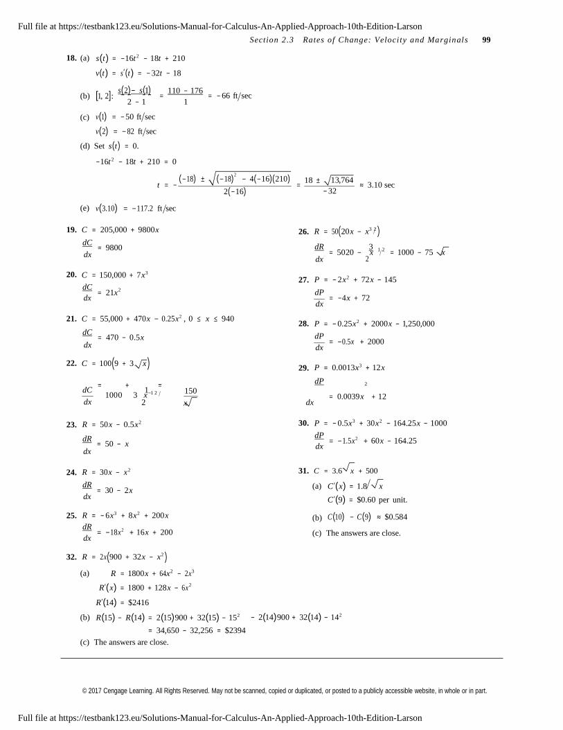
18. (a) s(t) = −16t 2 − 18t + 210
v(t ) = s′(t ) = − 32t − 18
s(2)− s(1) (b) [1, 2]:
110 − 176 = = − 66 ft sec
(c)
2 − 1 1
v(1) = − 50 ft sec
v(2) = −82 ft sec
(d) Set s(t ) = 0.
−16t 2 − 18t + 210 = 0
(−18) ±
(−18)2
− 4(−16)(210)
18 ±
13,764
t = − = ≈ 3.10 sec
(e)
v(3.10) = −117.2 ft sec
2(−16) − 32
19. C = 205,000 + 9800x 26. R = 50(20 x − x3 2 )dC
= 9800 dR 3 1 2
dx dx
= 5020 − 2 x
= 1000 − 75 x
20.
C = 150,000 + 7 x3
27.
P = − 2x2 + 72x − 145
dC = 21x2
dx
dP = −4 x + 72
dx
21.
C = 55,000 + 470 x − 0.25x2 , 0 ≤ x ≤ 940 28.
P = − 0.25x2 + 2000x − 1,250,000
dC = 470 − 0.5x
dx
dP = −0.5x + 2000
dx
22. C = 100(9 + 3 x ) 29.
P = 0.0013x3 + 12x
=
+
=
dP 2
dC 1 1000 3 x
−1 2 150 = 0.0039 x
+ 12
dx
2 x dx
23. R = 50 x − 0.5x2 30. P = − 0.5x3 + 30 x2 − 164.25x − 1000
dR
= 50 − x dx
dP = −1.5x2 + 60x − 164.25
dx
24. R = 30 x − x2 31. C = 3.6 x + 500
dR = 30 − 2 x (a) C′(x) = 1.8 x
25.
dx
R = − 6 x3 + 8x2 + 200x
(b)
C′(9) = $0.60 per unit.
C(10) − C(9) ≈ $0.584
dR = −18x2 + 16 x + 200
dx
(c) The answers are close.
32.
R = 2x(900 + 32x − x2 )
(a)
(b)
R = 1800x + 64 x2 − 2x3
R′(x) = 1800 + 128x − 6x2
R′(14) = $2416
R(15) − R(14) = 2(15)900 + 32(15) − 152
= 34,650 − 32,256 = $2394
− 2(14)900 + 32(14) − 142
(c) The answers are close.
Full file at https://testbank123.eu/Solutions-Manual-for-Calculus-An-Applied-Approach-10th-Edition-Larson
Full file at https://testbank123.eu/Solutions-Manual-for-Calculus-An-Applied-Approach-10th-Edition-Larson
© 2017 Cengage Learning. All Rights Reserved. May not be scanned, copied or duplicated, or posted to a publicly accessible website, in whole or in part.
100 Chapte r 2 Differentiat i on
33. P = − 0.04 x2 + 25x − 1500
(a)
dP = − 0.08x + 25 = P′(x)
dx
P′(150) = $13
(b)
Δ P = P(151) − P(150)
1362.96 − 1350 =
= $12.96
Δ x 151 − 150 1
(c) The results are close.
34.
P = 36,000 + 2048 x − 1
, 150 ≤ x ≤ 275 8x2
dP 1 = 2048 x
−1 2
− 1(−2x−3 )
dx 2
8
= 1024
+ 1
x 4x3
(a) When x = 150, dP dx
(d) When x = 225, dP dx
≈ $83.61.
≈ $68.27.
(b) When x = 175, dP dx
(e) When x = 250, dP dx
≈ $77.41.
≈ $64.76.
(c) When x = 200, dP dx
(f ) When x = 275, dP dx
≈ $72.41.
≈ $61.75.
35.
P = 1.73t 2 + 190.6t + 16,994
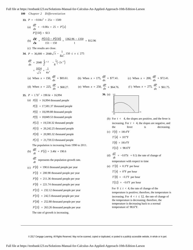
36. (a) 103
(a) P(0) = 16,994 thousand people
P(3) = 17,581.37 thousand people
P(6) = 18,199.88 thousand people
0 15
98
P(9) = 18,849.53 thousand people
P(12) = 19,530.32 thousand people
P(15) = 20,242.25 thousand people
(b) For t < 4, the slopes are positive, and the fever is
increasing. For t > 4, the slopes are negative, and
the fever is decreasing.
P(18) = 20,985.32 thousand people
P(21) = 21,759.53 thousand people
The population is increasing from 1990 to 2011.
(c) T (0) = 100.4°F
T ′(4) = 101°F
T (8) = 100.4°F
T (12) = 98.6°F
(b)
(c)
dP = P′(t) = 3.46t + 190.6
dt
dP represents the population growth rate.
dt
P′(0) = 190.6 thousand people per year
P′(3) = 200.98 thousand people per year
P′(6) = 211.36 thousand people per year
P′(9) = 221.74 thousand people per year
P′(12) = 232.12 thousand people per year
P′(15) = 242.5 thousand people per year
P′(18) = 252.88 thousand people per year
P′(21) = 263.26 thousand people per year
The rate of growth is increasing.
(d)
(e)
dT
= −0.075t + 0.3; the rate of change of dt
temperature with respect to time
T ′(0) = 0.3°F per hour
T ′(4) = 0°F per hour
T ′(8) = −0.3°F per hour
T (12) = −0.6°F per hour
For 0 ≤ t < 4, the rate of change of the
temperature is positive; therefore, the temperature is
increasing. For 4 < t ≤ 12, the rate of change of
the temperature is decreasing; therefore, the
temperature is decreasing back to a normal
temperature of 98.6°F.
Full file at https://testbank123.eu/Solutions-Manual-for-Calculus-An-Applied-Approach-10th-Edition-Larson
Full file at https://testbank123.eu/Solutions-Manual-for-Calculus-An-Applied-Approach-10th-Edition-Larson
© 2017 Cengage Learning. All Rights Reserved. May not be scanned, copied or duplicated, or posted to a publicly accessible website, in whole or in part.
Q 0 2 4 6 8 10
Model 160 120 80 40 0 −40
Table − 130 90 50 10 −30
x 600 1200 1800 2400 3000
dR dx 3.8 2.6 1.4 0.2 −1.0
dP dx 2.3 1.1 −0.1 −1.3 −2.5
P 1705 2725 3025 2605 1465
Section 2.3 Rates of C han ge: Velocity a nd Ma rgin al s 101
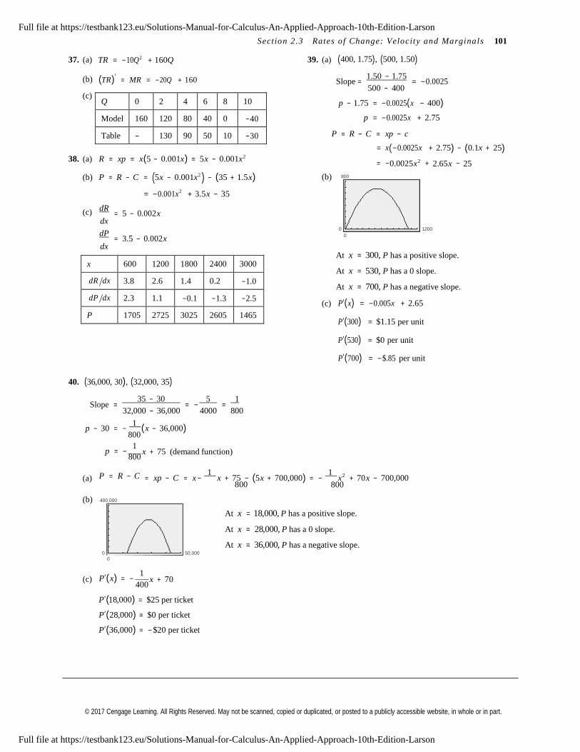
37. (a) TR = −10Q2 + 160Q 39. (a) (400, 1.75), (500, 1.50)
(b) (TR)′ = MR = −20Q + 160
(c)
Slope = 1.50 − 1.75
= −0.0025 500 − 400
p − 1.75 = −0.0025(x − 400)
p = −0.0025x + 2.75
P = R − C = xp − c
= x(−0.0025x + 2.75) − (0.1x + 25)38. (a) R = xp = x(5 − 0.001x) = 5x − 0.001x2
0.0025x2
2.65x 25
(b) P = R − C = (5x − 0.001x2 ) − (35 + 1.5x)
= −0.001x2 + 3.5x − 35
(b)
800
= − + −
(c)
dR
= 5 − 0.002 x dx
dP = 3.5 − 0.002 x
dx
0 1200
0
(c)
At x = 300, P has a positive slope.
At x = 530, P has a 0 slope.
At x = 700, P has a negative slope.
P′(x) = −0.005x + 2.65
P′(300) = $1.15 per unit
P′(530) = $0 per unit
P′(700) = −$.85 per unit
40. (36,000, 30), (32,000, 35)
Slope = 35 − 30
= − 5
= 1
32,000 − 36,000 4000 800
p − 30 = − 1
(x − 36,000) 800
(a)
p = − 1
800
P = R − C
x + 75 (demand function)
= xp − C = x −
1 x + 75
− (5x + 700,000) = −
1 x2 + 70 x − 700,000
800
800 (b)
400,000
At x = 18,000, P has a positive slope.
At x = 28,000, P has a 0 slope.
At x = 36,000, P has a negative slope.0 50,000
0
(c)
P′(x) = − 1
400
x + 70
P′(18,000) = $25 per ticket
P′(28,000) = $0 per ticket
P′(36,000) = − $20 per ticket
Full file at https://testbank123.eu/Solutions-Manual-for-Calculus-An-Applied-Approach-10th-Edition-Larson
Full file at https://testbank123.eu/Solutions-Manual-for-Calculus-An-Applied-Approach-10th-Edition-Larson
© 2017 Cengage Learning. All Rights Reserved. May not be scanned, copied or duplicated, or posted to a publicly accessible website, in whole or in part.
x 10 15 20 25 30 35 40
C 3900 2600 1950 1560 1300 1114.29 975
dC dx − 390 −173.33 − 97.5 − 62.4 − 43.33 − 31.84 − 24.38
102 Chapte r 2 Differentiat i on
41. (a)
C(x) = 15,000 mi 1 gal 2.60 dollars
yr
x mi
1 gal
C(x) = 39,000 dollars
x yr
dollars
dC 39,000 yr(b) = −
dx x2
mpg
(c)
The marginal cost is the change of savings for a 1-mile per gallon increase in fuel efficiency.
(d) The driver who gets 15 miles per gallon would benefit more than the driver who gets 35 miles per gallon.
The value of dC dx is a greater savings for x = 15 than for x = 35.
42. (a) f ′(2.959) is the rate of change of the number of gallons of gasoline sold when the price is $2.959 gallon.
(b) In general, it should be negative. Demand tends to decrease as price increases. Answers will vary.
43. (a) Average rate of change from 2000 to 2013: Δ p Δt
= 16,576.66 − 10,786.85
≈ $445.37 yr 13 − 0
(b) Average rate of change from 2003 to 2007: Δ p Δt
= 13,264.82 − 10,453.92
7 − 3
≈ $702.73 yr
So, the instantaneous rate of change for 2005 is p′(5) ≈ $702.73 yr.
(c) Average rate of change from 2004 to 2006: Δ p Δt
= 12,463.15 − 10,783.01
≈ $840.07 yr 6 − 4
So, the instantaneous rate of change for 2005 is p′(5) ≈ $840.07 yr.
(d) The average rate of change from 2004 to 2006 is a better estimate because the data is closer to the years in question.
44. Answers will vary. Sample answer:
The rate of growth in the lag phase is relatively slow when compared with the rapid growth in the acceleration phase.
The population grows slower in the deceleration phase, and there is no growth at equilibrium. These changes could be
explained by food supply or seasonal growth.
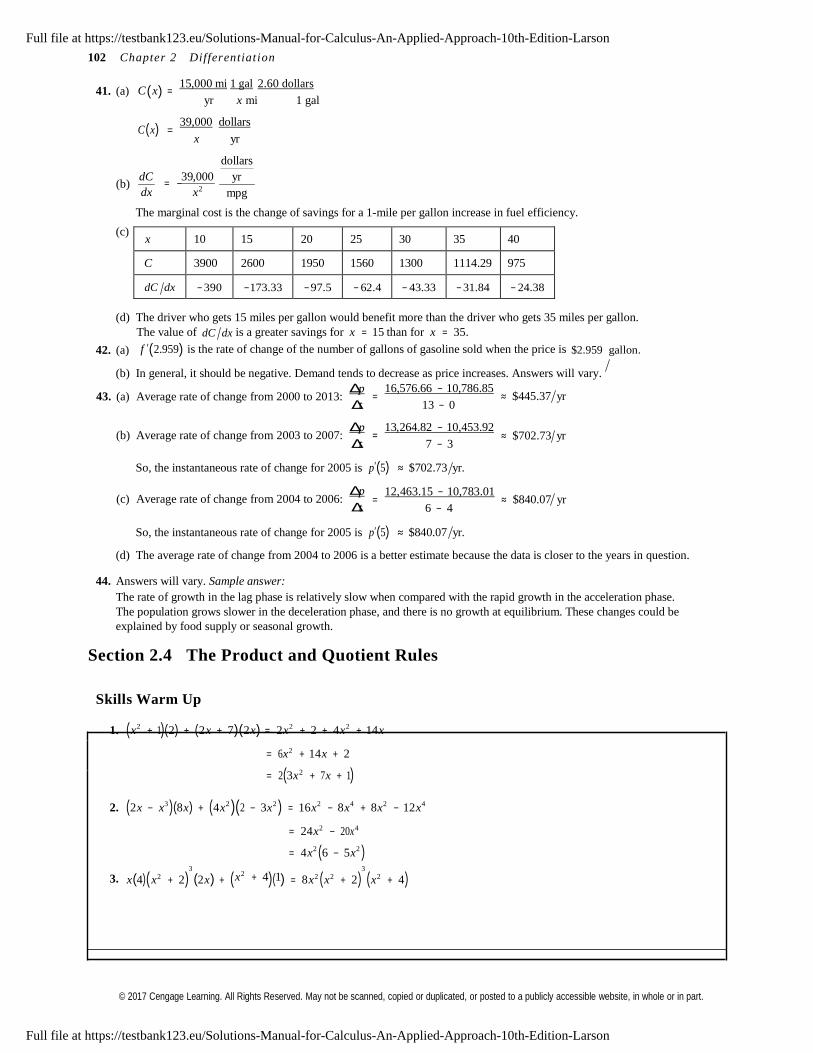
Section 2.4 The Product and Quotient Rules
Skills Warm Up
1. (x2 + 1)(2) + (2 x + 7)(2x) = 2x2 + 2 + 4x2 + 14x
= 6 x2 + 14x + 2
= 2(3x2 + 7 x + 1)
2. (2x − x3 )(8x) + (4x2 )(2 − 3x2 ) = 16x2 − 8x4 + 8x2 − 12x4
= 24x2 − 20 x4
= 4x2 (6 − 5x2 ) 3
x 4 x2 + 2 2 x + x2 + 4 1 3
= 8x2 x2 + 2 x2 + 43. ( )( ) ( ) ( )( ) ( ) ( )
Full file at https://testbank123.eu/Solutions-Manual-for-Calculus-An-Applied-Approach-10th-Edition-Larson
Full file at https://testbank123.eu/Solutions-Manual-for-Calculus-An-Applied-Approach-10th-Edition-Larson
© 2017 Cengage Learning. All Rights Reserved. May not be scanned, copied or duplicated, or posted to a publicly accessible website, in whole or in part.
2
2
2
2 2
Section 2.4 The Product and Quotient Rules 103
Skills Warm Up —continued—
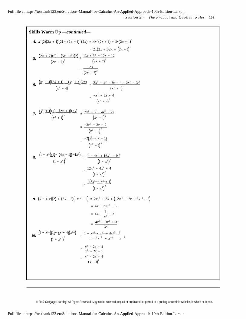
4. x2 (2)(2 x + 1)(2) + (2 x + 1)4 (2 x) = 4x2 (2x + 1) + 2 x(2x + 1)
4
= 2x(2x + 1)2 x + (2x + 1)3
5. (2 x + 7)(5) − (5 x + 6)(2)
(2x + 7)2
= 10 x + 35 − 10 x − 12
(2x + 7)2
= 23
(2 x + 7)2
( x2 − 4)(2 x + 1) − ( x2 + x)(2 x) 6.
2 =
2 x3 + x2 − 8 x − 4 − 2 x3 − 2 x2
2
(x2 − 4) (x2 − 4) − x2 − 8x − 4
=
(x2 − 4)
( x2 + 1)(2)− (2 x + 1)(2 x) 7.
2 =
2 x2 + 2 − 4 x2 − 2 x
2
(x2 + 1) (x2 + 1) −2x2 − 2 x + 2
=
(x2 + 1)
−2( x2 + x − 1)=
(x2 + 1)
(1 − x4 )(4)− (4 x − 1)(−4 x3 ) 8.
2 =
4 − 4 x4 + 16 x4 − 4 x3
2
(1 − x4 ) (1 − x4 ) 12 x4 − 4x3 + 4
=
(1 − x4 )2
4(3x4 − x3 + 1) =
(1 − x4 )2
9. (x−1 + x)(2) + (2 x − 3)(− x−2 + 1) = 2x−1 + 2x + (−2x−1 + 2 x + 3x−2 − 3) = 4x + 3x−2 − 3
= 4x + 3
− 3 x2
4x3 − 3x2 + 3 =
x2
(1 − x−1 )(1) − ( x − 4)( x−2 )
1 − x−1 − x−1 + 4 x−2 x2
10.
(1 − x−1 ) =
1 − 2x−1 + x−2
x
x2 − 2 x + 4 =
x2 − 2 x + 1
x2 − 2 x + 4 =
(x − 1)2
Full file at https://testbank123.eu/Solutions-Manual-for-Calculus-An-Applied-Approach-10th-Edition-Larson
Full file at https://testbank123.eu/Solutions-Manual-for-Calculus-An-Applied-Approach-10th-Edition-Larson
© 2017 Cengage Learning. All Rights Reserved. May not be scanned, copied or duplicated, or posted to a publicly accessible website, in whole or in part.
104 Chapte r 2 Differentiat i on
Skills Warm Up —continued—
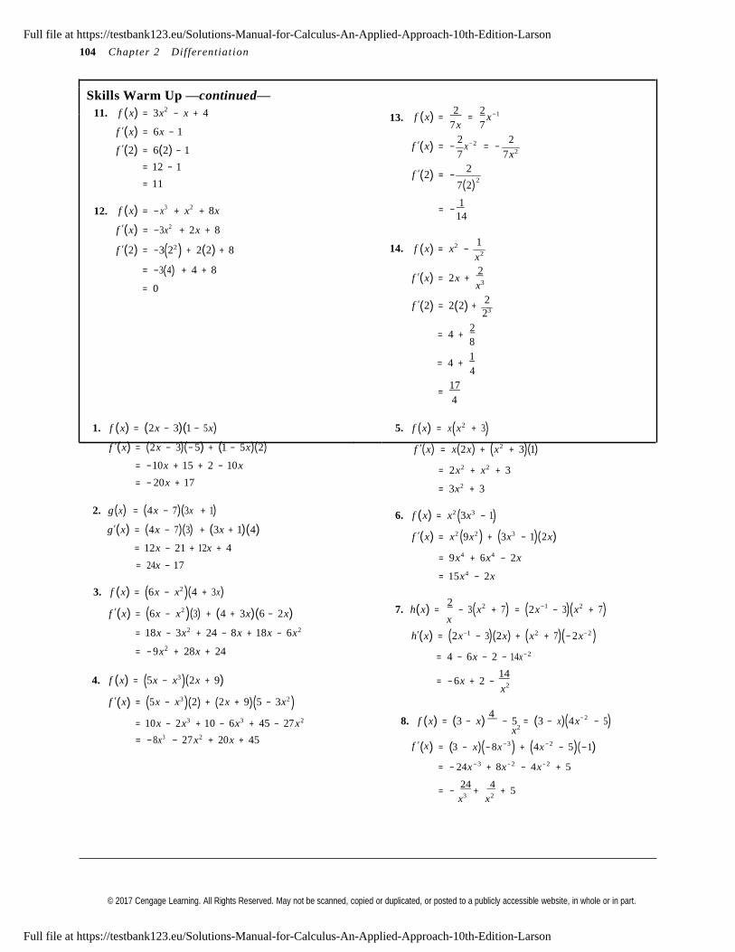
11. f (x) = 3x2 − x + 4
f ′(x) = 6x − 1
13. f (x) = 2
= 7 x
2 x−1
7
2 2f ′(2) = 6(2) − 1
f ′(x) = − x− 2 = −
= 12 − 1 7 7 x2
2f ′(2) = −
2
12.
= 11
f (x) = −x3 + x2 + 8x
f ′(x) = −3x2 + 2x + 8
7(2)
1 = −
14
f ′(2) = −3(22 ) + 2(2) + 8 14. f (x) = x2 − 1 x2
= −3(4) + 4 + 8
= 0 f ′(x) = 2x +
2 x3
2f ′(2) = 2(2) +
23
= 4 + 2 8
= 4 + 1 4
= 17 4
1. f (x) = (2x − 3)(1 − 5x)
f ′(x) = (2 x − 3)(− 5) + (1 − 5x)(2)
= −10 x + 15 + 2 − 10 x
= − 20x + 17
2. g (x) = (4 x − 7)(3x + 1)
g′(x) = (4 x − 7)(3) + (3x + 1)(4)
= 12x − 21 + 12 x + 4
= 24 x − 17
3. f (x) = (6 x − x2 )(4 + 3x)
f ′(x) = (6 x − x2 )(3) + (4 + 3x)(6 − 2 x)
5. f ( x) = x(x2 + 3) f ′(x) = x(2 x) + (x2 + 3)(1)
= 2x2 + x2 + 3
= 3x2 + 3
6. f (x) = x2 (3x3 − 1)
f ′(x) = x2 (9 x2 ) + (3x3 − 1)(2 x)
= 9x4 + 6 x4 − 2 x
= 15x4 − 2 x
7. h(x) = 2
− 3(x2 + 7) = (2 x−1 − 3)(x2 + 7) x
= 18x − 3x2 + 24 − 8x + 18x − 6 x2
= − 9 x2 + 28x + 24
4. f (x) = (5x − x3 )(2x + 9)
f ′(x) = (5x − x3 )(2) + (2 x + 9)(5 − 3x2 ) = 10 x − 2 x3 + 10 − 6 x3 + 45 − 27 x2
h′(x) = (2x−1 − 3)(2x) + (x2 + 7)(− 2 x− 2 ) = 4 − 6x − 2 − 14 x− 2
= − 6x + 2 − 14 x2
8. f (x) = (3 − x) 4
− 5
= (3 − x)(4x− 2 − 5) x2
= −8x3 − 27 x2 + 20 x + 45 ( ) ( )(
3 ) ( 2
)( )f ′ x = 3 − x − 8x− + 4 x−
− 5 −1
= − 24 x−3 + 8x− 2 − 4 x− 2 + 5
24 4 = − + + 5
x3 x2
Full file at https://testbank123.eu/Solutions-Manual-for-Calculus-An-Applied-Approach-10th-Edition-Larson
Full file at https://testbank123.eu/Solutions-Manual-for-Calculus-An-Applied-Approach-10th-Edition-Larson
© 2017 Cengage Learning. All Rights Reserved. May not be scanned, copied or duplicated, or posted to a publicly accessible website, in whole or in part.
2
2
2
2
2
2
Section 2.4 The Product and Quotient Rules 105
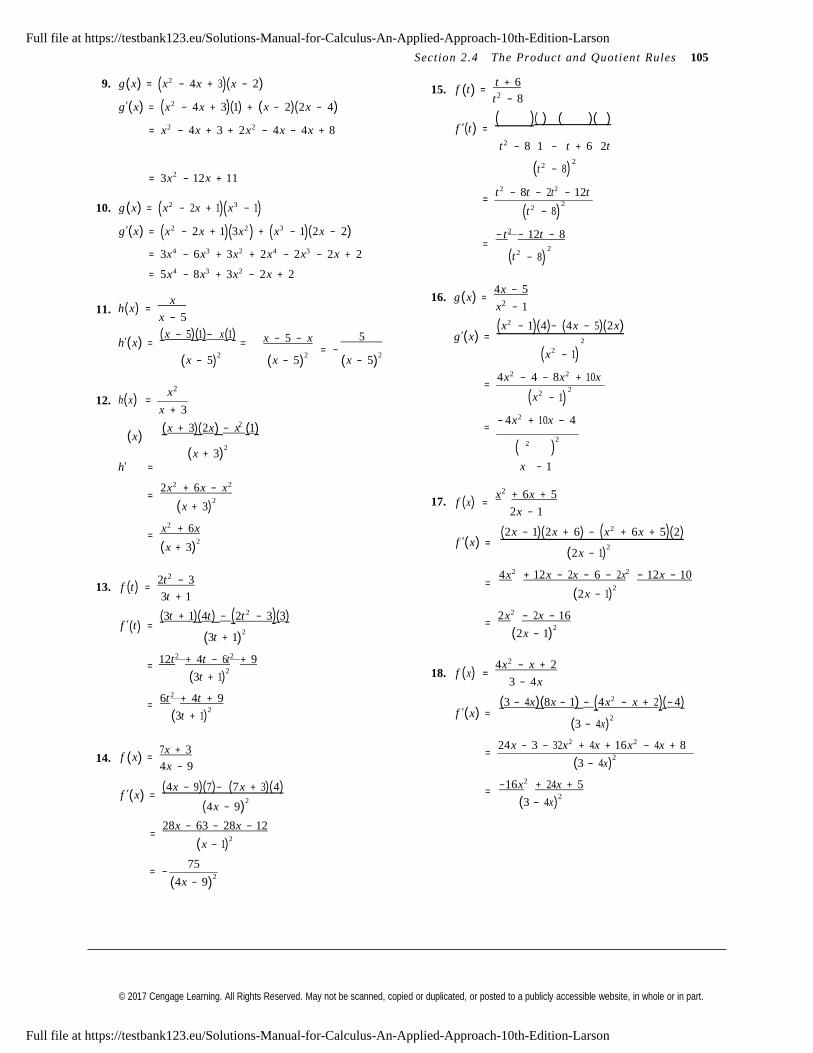
9. g (x) = (x2 − 4x + 3)(x − 2)
g′(x) = (x2 − 4x + 3)(1) + (x − 2)(2 x − 4)
= x2 − 4 x + 3 + 2x2 − 4x − 4x + 8
15. f (t) = t + 6 t 2 − 8
f ′(t ) = ( )( ) ( )( )
t 2 − 8 1 −
2
t + 6 2t
2
= 3x2 − 12x + 11 (t − 8)
10.
g (x) = (x2 − 2 x + 1)(x3 − 1)
g′(x) = (x2 − 2x + 1)(3x2 ) + (x3 − 1)(2x − 2)
t 2 − 8t − 2t 2 − 12t =
(t 2 − 8) − t 2 − 12t − 8
= 3x4 − 6x3 + 3x2 + 2x4 − 2 x3 − 2x + 2
= 5x4 − 8x3 + 3x2 − 2x + 2
=
(t 2 − 8)
11.
h(x) = x
x − 5
h′(x) = ( x − 5)(1)− x(1)
=
x − 5 − x
5
= −
16. g(x) =
g′(x) =
4 x − 5
x2 − 1
( x2 − 1)(4)− (4 x − 5)(2 x) 2
(x − 5)2
(x − 5)2
(x − 5)2
(x2
− 1)
4x2 − 4 − 8x2 + 10 x
12.
h(x) = x2
x + 3
=
(x2 − 1)
− 4 x2 + 10 x − 4
(x) ( x + 3)(2 x) − x (1) =
( 2 )h′ =
(x + 3)2
x − 1
13.
=
=
f (t ) =
2 x 2 + 6 x − x 2
(x + 3)2
x 2 + 6 x
(x + 3)2
2t 2 − 3
3t + 1
17.
f (x) =
f ′(x) =
=
x 2 + 6 x + 5
2x − 1
(2 x − 1)(2 x + 6) − ( x2 + 6 x + 5)(2)
(2x − 1)2
4 x 2 + 12 x − 2 x − 6 − 2 x 2 − 12 x − 10
(2x − 1)2
( ) (3t + 1)(4t ) − (2t − 3)(3) 2 x 2 − 2 x − 16
f ′ t =
(3t + 1)2
= (2x − 1)
2
12t 2 + 4t − 6t 2 + 9 =
(3t + 1)2
6t 2 + 4t + 9 =
(3t + 1)2
18.
f (x) =
f ′(x) =
4 x2 − x + 2
3 − 4x
(3 − 4 x)(8x − 1) − (4 x 2 − x + 2)(− 4)
(3 − 4 x)2
24 x − 3 − 32 x2 + 4 x + 16x2 − 4 x + 814. f (x) =
7 x + 3
4x − 9
f ′(x) = (4 x − 9)(7)− (7 x + 3)(4)
(4 x − 9)2
= (3 − 4 x)
2
−16 x 2 + 24 x + 5 =
(3 − 4 x)2
= 28x − 63 − 28x − 12
(x − 1)2
= − 75
(4x − 9)2
Full file at https://testbank123.eu/Solutions-Manual-for-Calculus-An-Applied-Approach-10th-Edition-Larson
Full file at https://testbank123.eu/Solutions-Manual-for-Calculus-An-Applied-Approach-10th-Edition-Larson
© 2017 Cengage Learning. All Rights Reserved. May not be scanned, copied or duplicated, or posted to a publicly accessible website, in whole or in part.
x
106 Chapte r 2 Dif ferentiat i on
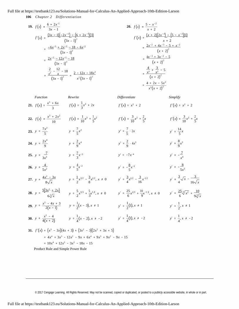
19. f (x) = 6 + 2x−1
3x − 1
20. f (x) = 5 − x− 2
x + 2
′(x) = (3x − 1)(− 2 x ) − (6 + 2 x )(3)
( x + 2)(2 x ) − (5 − x )(1) − 2 −1
f
(3x 1)2 f ′(x) =
−3 − 2
x + 2− − 2 −3 − 2
− 6 x −1 + 2 x − 2 − 18 − 6 x −1
= (3x − 1)
2
= 2 x + 4 x − 5 + x
(x + 2)2
−3 − 2
2 x − 2 − 12 x −1 − 18 =
(3x − 1)2
= 4 x + 3x − 5
(x + 2)2
4 +
3 − 52
− 12
− 18 3 2
= x 2 x
=
(3x − 1)2
2 − 12 x − 18 x2
x2 (3x − 1)2
= x x
(x + 2)2
4 + 2 x − 5x3
= x3 (x + 2)
2
Function Rewrite Differentiate Simplify
21.
f (x) = x3 + 6 x
3
f (x) = 1
x3 + 2x 3
f ′(x) = x2 + 2
f ′(x) = x2 + 2
22. f (x) = x3 + 2x2
10
f (x) = 1
x3 + 1 x2
10 5
f ′(x) = 3
x2 + 2 x
10 5
f ′(x) = 3
x2 + 2 x
10 5
23.
7 x2
y = 5
2x4
y = 7
x2
5
2
y' = 7
⋅ 2x 5
2
y′ =
14
x 5
8
24. y = 9
7
y = x4
9
7 −3
y′ = ⋅ 4x3
9
−4
y′ = x3
9
7 25. y =
3x3
y = x 3
y' = −7 x y′ = − x4
26.
y = 4 5x2
y = 4
x−2
5
8 y′ = − −3
5
8 y′ = −
5x3
27.
4 x2 − 3x
y =
y = 1 x3 2 −
3
x1 2
, x ≠ 0
y′ =
3
x1 2 −
3
x−1 2
y′ =
3
x − 3
8 x 2 8 4 16 4 16 x
5(3x2 + 2 x)
25 10 28. y = y =
5 x5 3 +
5 x5 3 , x ≠ 0 y′ = 25
x2 3 + 10
x−1 3 , x ≠ 0 y′ = 3 x2 +
29.
6 3 x
x2 − 4 x + 3 y =
2(x − 1)
2 3
y = 1 (x − 3), x ≠ 1
2
y′ =
6 9 1 (1), x ≠ 1
2
y′ =
6 9 3 x
1 , x ≠ 1
2
30. x2 − 4
y = 4(x + 2)
y = 1 4
(x − 2), x ≠ − 2
y′ = 1 (1), x ≠ − 2
4
y′ = 1
, x ≠ − 2 4
31. f ′(x) = (x3 − 3x)(4x + 3) + (3x2 − 3)(2 x2 + 3x + 5) = 4x4 + 3x3 − 12 x2 − 9x + 6x4 + 9x3 + 9 x2 − 9x − 15
= 10x4 + 12x3 − 3x2 − 18x − 15
Product Rule and Simple Power Rule
Full file at https://testbank123.eu/Solutions-Manual-for-Calculus-An-Applied-Approach-10th-Edition-Larson
Full file at https://testbank123.eu/Solutions-Manual-for-Calculus-An-Applied-Approach-10th-Edition-Larson
© 2017 Cengage Learning. All Rights Reserved. May not be scanned, copied or duplicated, or posted to a publicly accessible website, in whole or in part.
3
2
3
2
2
2
2
2
2
Section 2.4 The Product and Quotien t Rules 107
32. h′(t ) = (t 5 − 1)(8t − 7) + (5t 4 )(4t 2 − 7t − 3) 35.
(x 2 − 1) (3x2 + 3) − (x3 + 3x + 2) (2 x) f ′(x) =
= 8t 6 − 7t 5 − 8t + 7 + 20t 6 − 35t 5 − 15t 4 (x2 − 1)
33.
= 28t 6 − 42t 5 − 15t 4 − 8t + 7
Product Rule and Simple Power Rule
h(t ) = 1 (6t − 4)
3x4 − 3 − 2x4 − 6 x2 − 4x =
(x2 − 1) x4 − 6 x2 − 4 x − 3
=
h′(t ) = 1 (6) = 2 (x2 − 1)
Constant Multiple and Simple Power Rules Quotient Rule and Simple Power Rule
34.
f (x) =
1 (3x − 8)
2 x 3 − 4 x 2 − 9
f x =
f ′(x) = 2
1 (3) = 3
36. ( ) x3 − 5
2 2
Constant Multiple and Simple Power Rules ( x 3 − 5)(3x 2 − 8x) − (2 x 3 − 4 x 2 − 9)(3x 2 ) f ′(x) =
(x3 − 5)
3x5 − 8x4 − 15x2 + 40x − 6 x5 + 12 x4 − 27 x2
=
(x3 − 5)
−3x5 + 4x4 − 42x2 + 40x=
(x3 − 5)
37.
f (x) = 20
= ( )( )
= x − 5, x ≠ − 4
Quotient Rule and Simple Power Rule
x2 − x − x − 5 x + 4
f ′(x) = 1
x + 4 (x + 4)
38.
Simple Power Rule
h(t) = 3 22 7
= ( )( )
= 3t + 1, t ≠ − 7
t 2 + t +
t + 7
3t + 1 1 + 7
t + 7
h′(t) = 3, t ≠ −7
Simple Power Rule
39. g (t) = (2t 3 − 1) = (2t 3 − 1)(2t 3 − 1)
g′(t) = (2t 3 − 1)(6t 2 ) + (2t 3 − 1)(6t 2 )
= 12t 2 (2t 3 − 1)
Product Rule and Simple Power Rule
f x = 2
4 x3 − 2 x − 3 = 4 x3 − 2 x − 3 4 x3 − 2 x − 340. ( ) ( ) ( )( )
f ′(x) = (4x3 − 2x − 3)(12 x2 − 2) + (4x3 − 2x − 3)(12 x2 − 2)
= 48x5 − 24x3 − 36 x2 − 8x3 + 4 x + 6 + 48x5 − 24 x3 − 36x2 − 8x3 + 4 x + 6
= 96 x5 − 48x3 − 72x2 − 16x3 + 8x + 12
Product Rule and Simple Power Rule
Full file at https://testbank123.eu/Solutions-Manual-for-Calculus-An-Applied-Approach-10th-Edition-Larson
Full file at https://testbank123.eu/Solutions-Manual-for-Calculus-An-Applied-Approach-10th-Edition-Larson
© 2017 Cengage Learning. All Rights Reserved. May not be scanned, copied or duplicated, or posted to a publicly accessible website, in whole or in part.
2
2
108 Chapte r 2 Dif ferentiat i on
41.
g (s) = s 2 − 2s + 5
= s
s 2 − 2s + 5
s1 2
45. f (x) = (x + 4)(2 x + 9)(x − 3)
( )
s1 2(2s − 2) − ( s 2 − 2s + 5)( 1 s −1 2 ) = 2 x2 + 17 x + 36 (x − 3)
g′(s) = 2
s f ′(x) = (2x2 + 17 x + 36)(1) + (x − 3)(4 x + 17)
2s3 2 − 2s1 2 − 1 s3 2 + s1 2 − 5 s−1 2
= 2 2
s
3 5 3s2 − 2s − 5
= (2x2 + 17 x + 36) + (4 x2 + 5x − 51) = 6 x2 + 22x − 15
= s1 2 − s −1 2 − s−3 2 = Product Rule and Simple Power Rule2 2 2s3 2
Quotient Rule and Simple Power Rule
x3 − 5 x2 − 6 x x3 − 5x2 − 6 x
46. f (x) = (3x3 + 4x)(x − 5)(x + 1)
= (3x3 + 4x)(x2 − 4x − 5) 3 2 242. f (x) = =
x x1 2
f ′(x) = (3x + 4x)(2 x − 4) + (x − 4 x − 5)(9 x + 4)
= x5 2 − 5x3 2 − 6x1 2
= (6 x4 − 12 x3 + 8x2 − 16 x)
f ′(x) = 5
x3 2 − 15
x1 2 − 3x−1 2
+ (9 x
− 36 x
− 41x
− 16 x − 20)2 2
= 5
x3 2 − 15
x1 2 − 3
4 3 2
= 15x4 − 48x3 − 33x2 − 32x − 20
Product Rule and Simple Power Rule2 2
5 x 2 − 15 x − 6 =
2 x1 2
x 1 2
47.
f (x) = (5x + 2)(x2 + x)
Constant Multiple and Simple Power Rules f ′(x) = (5x + 2)(2 x + 1) + (x2 + x)(5)
= 10 x2 + 9 x + 2 + 5x2 + 5x
43. f (x) = ( x − 2)( 3x + 1) 3x 2 − 5x − 2
= 10
= 15x2 + 14 x + 24x + 2 4x + 2
( ) (4 x + 2)(6 x − 5) − (3x − 5 x − 2)(4)
m = f ′(−1) = 3
(− 1, 0) − 5 5
f ′ x = (4 x + 2)
2
y − 0 = 3(x − (−1))
24x2 − 8x − 10 − 12x2 + 20x + 8 =
(4 x + 2)2
12 x 2 + 12 x − 2 =
48.
y = 3x + 3
f (x) = (x2 − 1)(x3 − 3x)
− 10
4(2x + 1)2
( ) ( 2
)( 2
) ( 2
)( )f ′ x = x − 1 3x − 3 + x − 3x 2 x
2(6x 2 + 6 x − 1) =
2(2x + 1)2
= 3x4 − 6x2 + 3 + 2 x4 − 6x2
4 2
6 x2 + 6x − 1
= 5x − 12x + 3
= 2(2x + 1)
2
m = f ′(− 2) = 5(− 2)4
− 12(− 2)2
+ 3 = 35
Quotient Rule and Simple Power Rule y − (− 6) = 35(x − (− 2))
y + 6 = 35x + 70
44. f (x) = ( x + 1)( 2x − 7)
= 2 x 2 − 5x − 7 y = 35x + 64
2x + 1 2x + 1
( ) (2 x + 1)(4 x − 5) − (2 x − 5x − 7)(2)
2
−6 6
f ′ x = (2 x + 1)
2
8x2 − 6x − 5 − 4x2 + 10x + 14 =
(2 x + 1)2
4x2 + 4 x + 9 =
(2x + 1)2
(−2, −6)
−8
Quotient Rule and Simple Power Rule
Full file at https://testbank123.eu/Solutions-Manual-for-Calculus-An-Applied-Approach-10th-Edition-Larson
Full file at https://testbank123.eu/Solutions-Manual-for-Calculus-An-Applied-Approach-10th-Edition-Larson
© 2017 Cengage Learning. All Rights Reserved. May not be scanned, copied or duplicated, or posted to a publicly accessible website, in whole or in part.
(9, 18)
2
2 2
−
2
10
=
Section 2.4 The Product and Quotien t Rules 109
49. f (x) = x3 (x2 − 4) 50. f (x) = x (x − 3) = x1 2 (x − 3)
f ′(x) = x2 (2x) + (x2 − 4)(3x2 )
= 2 x4 + 3x4 − 12 x2
f ′(x) = x1 2 (1) + (x − 3)(1 x−1 2 )
= x1 2 + 1 x1 2 − 3 x−1 2
= 5x4 − 12 x2
m = f ′(1) = − 7 − 5
3 x1 2 3 x− 1 2 2 2
5(1, − 3) m = f ′(9) = 3 (9)
1 2 − 3 (9)
−1 2 = 9 − 1 = 4
y − (−3) = − 7(x − 1)
y = − 7 x + 4
− 10
2 2 2 2
y − 18 = 4(x − 9)
y = 4 x − 18
10
51.
f (x) = 3x − 2 x + 1
f ′(x) = ( x + 1)(3) − (3x − 2)(1)
0 20
0
= 3x + 3 − 3x + 2
= 5
f ′(4) = 1
5
(x + 1)2 (x + 1)
2 (x + 1)
2
y − 2 = 1 (x − 4)
5
y − 2 = 1 x −
4 5 5
y = 1
x + 6
5 5
4
(4, 2)
− 2 10
− 4
52.
f ′(x) =
( x − 1)2 − (2 x + 1) =
−3 53. (x)
(3x − 2)(6 x + 5) 18x 2 + 3x − 10f = =
(x − 1)2
(x − 1)2 2x − 3 2x − 3
f ′(2) = −3
( ) (2 x − 3)(36 x + 3) − (18 x + 3x − 10)(2)
y − 5 = −3(x − 2) f ′ x =
(2x − 3)2
y = −3x + 11
8
(2, 5)
72 x2 − 102 x − 9 − 36 x2 − 6 x − 20 =
(2x − 3)2
36x2 − 108x + 11 =
(2x − 3)2
−7 8
36(−1) 2
− 108(−1) + 11 31 m = f ′(−1) = =
−2 (2(−1) − 3)2 5
y − (−1) = 31
(x − (−1)) 10
5
y = 31
x + 26
5 5 − 5 (− 1, − 1)
5
− 10
Full file at https://testbank123.eu/Solutions-Manual-for-Calculus-An-Applied-Approach-10th-Edition-Larson
Full file at https://testbank123.eu/Solutions-Manual-for-Calculus-An-Applied-Approach-10th-Edition-Larson
© 2017 Cengage Learning. All Rights Reserved. May not be scanned, copied or duplicated, or posted to a publicly accessible website, in whole or in part.
2 3 2
2 2
2 3 4
− 2 2
2
2
110 Chapte r 2 Dif ferentiat i on
54. f (x) =
( x + )( x + x) =
2 2 x3 + 3x2 + 2 x
x − 4 x − 4
( ) ( x − 4)(3x + 6 x + 2) − ( x + 3x + 2 x)(1)
f ′ x = (x − 4)
2
3x3 − 12x2 + 6 x2 − 24 x + 2x − 8 − x3 − 3x2 − 2x =
(x − 4)2
2 x3 − 9x2 − 24x − 8 =
(x − 4)2
m = f ′(1) =
2(1)3 − 9(1)
2 − 24(1)− 8 13
= − 4
(1 − 4)2
y − (− 2) = − 13
(x − 1) 3
y = 13
x + 7
3 3
3
− 8 4
(1, −2)
− 4
55. ( ) ( x − 1)(2 x) − x (1)
x − 2 x
59. f (x) = x(x + 1) = x + x
2 2 2
f ′ x = =(x − 1)
2 (x − 1)
2 f ′(x) = 2x + 1
f ′(x) = 0 when x2 − 2 x = x(x − 2) = 0, which
implies that x = 0 or x = 2. Thus, the horizontal
tangent lines occur at (0, 0) and (2, 4).
6
f
− 2 2
56. ( ) ( x + 1)(2 x) − ( x )(2 x)
f ′
2 x − 3f ′ x = 2
2 =
2 2
(x + 1) (x + 1)
60.
f (x) = x2 (x + 1) = x3 + x2
f ′(x) = 0 when 2x = 0, which implies that x = 0.
Thus, the horizontal tangent line occurs
at (0, 0).
f ′(x) = 3x2 + 2x = x(3x + 2) 3
f ′ f
57. ( ) ( x + 1)(4 x ) − x (3x )
x + 4 x −2 2
3 3 4 2 6 3
f ′ x = 2
= 2
(x3 + 1) (x3 + 1)
f ′(x) = 0 when x6 + 4 x3
implies that x = 0 or x =
= x3 (x3 + 4) = 0, which
3 −4. Thus, the horizontal
61.
−1
f (x) = x(x + 1)(x − 1) 11
3
tangent lines occur at (0, 0) and ( 3 −4 , − 2.117).
58. ( ) ( x + 1)(4 x ) − ( x + 3)(2 x)
= x − x f ′
f ′(x) = 3x2 − 1
f
f ′ x =
(x2
− 6
+ 1)
2 x( x2 + 3)( x2 − 1) 62. f (x) = x2 (x + 1)(x − 1) = x4 − x2
=
(x2 + 1) f ′(x) = 4x
3 − 2x = 2 x(2 x2
3
− 1)
f ′(x) = 0 when 2 x(x2 + 3)(x2 − 1) = 0, which
implies that x = 0 or x = ±1. Thus, the horizontal
tangent lines occur at (0, 3), (1, 2), and (−1, 2).
f ′ f
−2 2
−1
Full file at https://testbank123.eu/Solutions-Manual-for-Calculus-An-Applied-Approach-10th-Edition-Larson
Full file at https://testbank123.eu/Solutions-Manual-for-Calculus-An-Applied-Approach-10th-Edition-Larson
© 2017 Cengage Learning. All Rights Reserved. May not be scanned, copied or duplicated, or posted to a publicly accessible website, in whole or in part.
2
2
2
2
2 2
2 2
Section 2.4 The Product and Quotien t Rules 111
63.
3 p x = 2751 −
66.
dP 50(t + 2)(1) − (t + 1750)(50) =
2
5 p + 1 dt 50(t + 2)
dx (5 p + 1)3 − (3 p)(5)
275 3
275 50(t + 2) − (t + 1750)
= − = − =dp (5 p + 1)
2
(5 p + 1) 2500(t + 2)2
= −1748
When
p = 4, dx 3
= −275 2
≈ −1.87 units dp (21)
50(t + 2)2
= −874
64.
per dollar.
dx
= 0 − 1 − dp
( p + 1)(2) − (2 p)(1)
( p + 1)2
25(t + 2)2
(a) When t = 1, dP dt
= −874
≈ −3.88 percent day. 225
= −1 − 2
( p + 1)2
−( p + 1)2
− 2
(b) When t = 10, dP dt
= −874 3600
437
= ( p + 1)
2
− p2 − 2 p − 3 =
( p + 1)2
67.
t 2 − t + 1 P =
t 2 + 1
= − 1800
≈ −0.24 percent day.
When
p = 3, dx
= −9 − 6 − 3
≈ −1.13 units
(t 2 1)(2t 1) (t 2 t 1)(2t ) dp 16 P′ = + − − − + t 2 − 1 =
per dollar. (t 2 + 1) (t 2 + 1)
(50 + t 2 )(4) − (4t )(2t ) 200 − 4t 2
(a) P′(0.5) = − 0.480 week
65. P′ = 500 = 500 (50 + t 2 ) (50 + t 2 ) (b) P′(2) = 0.120 week
184 When t = 2, P′ = 500 ≈ 31.55 bacteria hour.
(c)
P′(8) = 0.015 week
(54) Each rate in parts (a), (b), and (c) is the rate at which the
level of oxygen in the pond is changing at that particular
time.
68. T 4t 2 + 16t + 75 = 10
t 2 + 4t + 10
Initial temperature: T (0) = 75°F
2 2
′( )
(t + 4t + 10)(8t + 16) − (4t + 16t + 75)(2t + 4) − 700(t + 2) T t = 10
(t 2 + 4t + 10)
= (t 2
+ 4t + 10)
(a)
(b)
(c)
(d)
T ′(1) ≈ − 9.33°F hr
T ′(3) ≈ − 3.64°F hr
T ′(5) ≈ −1.62°F hr
T ′(10) ≈ − 0.37°F hr
Each rate in parts (a), (b), (c), and (d) is the rate at which the temperature of the food in the refrigerator
is changing at that particular time.
Full file at https://testbank123.eu/Solutions-Manual-for-Calculus-An-Applied-Approach-10th-Edition-Larson
Full file at https://testbank123.eu/Solutions-Manual-for-Calculus-An-Applied-Approach-10th-Edition-Larson
© 2017 Cengage Learning. All Rights Reserved. May not be scanned, copied or duplicated, or posted to a publicly accessible website, in whole or in part.
8
75
8 4
4 4
2
x
112 Chapte r 2 Dif ferentiat i on
69. C = x3 − 15x2 + 87 x − 73, 4 ≤ x ≤ 9 72. (a) P = ax2 + bx + c
Marginal cost: dC dx
= 3x2 − 30x + 87 When x = 10, P = 50: 50 = 100a + 10b + c.
When x = 12, P = 60: 60 = 144a + 12b + c.
Average cost: C = x2 − 15x + 87 −
73 When x = 14, P = 65: 65 = 196a + 14b + c.
x x Solving this system, we have
(a) 60
dC
dx
a = − 5 , b = 4
, and c = −75.
Thus, P = − 5 x2 + 75 x − 75.
C (b) 80
4 9
0
(b) Point of intersection:
3x2 − 30 x + 87 = x2 − 15x + 87 − 73 x
0 20
0
2 x2 − 15x + 73
= 0 x
(c) Marginal profit: P′ = − 5 x + 75 = 0 x = 15
2 x3 − 15x2 + 73 = 0
x ≈ 6.683
73.
This is the maximum point on the graph of P, so
selling 15 units will maximize the profit.
f (x) = 2 g (x) + h(x) When x = 6.683,
C =
dC ≈ 20.50.
x dx
Thus, the point of intersection is (6.683, 20.50).
At this point average cost is at a minimum.
70. (a) As time passes, the percent of people aware of the
product approaches approximately 95%.
(b) As time passes, the rate of change of the percent of
people aware of the product approaches zero.
74.
75.
f ′(x) = 2 g′(x) + h′(x)
f ′(2) = 2(−2) + 4 = 0
f (x) = 3 − g (x)
f ′(x) = −g′(x)
f ′(2) = −(−2) = 2
f (x) = g(x)h(x) 200 x
71. C = 100 x2
+ ,
x + 30
x ≥ 1 f ′(x) = g (x)h′(x) + h(x)g′(x)
C′ 100 2(200x−3 ) ( x + 30) − x
f ′(2) = g (2)h′(2) + h(2)g′(2)
= − +
(x + 30)2
= (3)(4) + (−1)(− 2)
= 14100
400 30
= − +
x3
′
(x + 30)2
400 30
76. f (x) = g(x) h(x)
(a) C (10) = 100 − 103
+ = −38.125 402
f ′ x h( x) g ′(x)− g (x)h′( x)
=(b) C′(15) ≈ −10.37
( ) h(x)
(c) C′(20) ≈ −3.8
Increasing the order size reduces the cost per item.
An order size of 2000 should be chosen since the
cost per item is the smallest at x = 20.
f ′(2) = (−1)(−2) − (3)(4)
(−1)2
77. Answers will vary.
= −10
Full file at https://testbank123.eu/Solutions-Manual-for-Calculus-An-Applied-Approach-10th-Edition-Larson
Full file at https://testbank123.eu/Solutions-Manual-for-Calculus-An-Applied-Approach-10th-Edition-Larson
© 2017 Cengage Learning. All Rights Reserved. May not be scanned, copied or duplicated, or posted to a publicly accessible website, in whole or in part.
Chapte r 2 Quiz Y oursel f 113
Chapter 2 Quiz Yourself 1. f (x) = 5x + 3 2. f (x) = x + 3
f ′(x) =
lim f ( x +Δx) − f ( x)
f ′(x) = f ( x +Δx) − f ( x) lim
Δx → 0 Δ x Δx → 0 Δx
= lim 5( x +Δx) + 3− (5x + 3) = lim x +Δx + 3 − x + 3
Δx → 0 Δ x Δx → 0 Δx
= lim 5x + 5Δ x + 3 − 5 x − 3 = lim
( )
x + Δx + 3 − x + 3Δx → 0 Δ x
Δx → 0 Δx( x + Δx + 3 + x + 3)
= lim 5Δ x = lim
1 Δx → 0 Δ x Δx → 0 x + Δx + 3 + x + 3
= lim 5 = 5 1 Δx → 0 =
At (− 2, − 7): m = 5 2 x + 3
At (1, 2): m = 1
= 1
2 1 + 3 4
3. f (x) = 3x − x2
f ′(x) =
=
=
=
=
=
=
lim Δx → 0
lim Δx → 0
lim Δx → 0
lim Δx → 0
lim Δx → 0
lim Δx → 0
lim Δx → 0
f ( x +Δx) − f ( x) Δ x
3(x + Δ x) − (x + Δ x)2 − (3x − x2 )
Δ x
3x + 3Δ x − ( x2 + 2 x(Δ x) + (Δ x)2 ) − (3x − x2 )
Δ x
3x + 3Δ x − x2 − 2 x(Δ x) − (Δ x)2
− 3x + x2
Δ x
3x − 2 x(Δ x) − (Δ x)2
Δ x
Δ x(3 − 2 x − Δ x) Δ x
(3 − 2x − Δ) = 3 − 2x
At (4, − 4): m = 3 − 2(4) = 3 − 8 = −5
4. f (x) = 12
f ′(x) = 0
5. f (x) = 19 x + 9
f ′(x) = 19
8. f (x) = 4x− 2
f ′(x) = −8x−3
9. f (x) = 10 x−1 5
8 = −
x3
+ x−3
6. f (x) = x4 − 3x3 − 5x2 + 8
f ′(x) = 4x3 − 9 x2 − 10 x
f ′(x) = −2 x− 6 5 − 3x− 4 = −
2 −
3 x− 6 5 x4
7. f (x) = 12x1 4
f ′(x) = 3x−3 4 = 3 x3 4
Full file at https://testbank123.eu/Solutions-Manual-for-Calculus-An-Applied-Approach-10th-Edition-Larson
Full file at https://testbank123.eu/Solutions-Manual-for-Calculus-An-Applied-Approach-10th-Edition-Larson
© 2017 Cengage Learning. All Rights Reserved. May not be scanned, copied or duplicated, or posted to a publicly accessible website, in whole or in part.
2
2
2
2
114 Chapte r 2 Dif ferentiat i on
10. f (x) = 2 x + 3
3x + 2
16. f (x) = 1
; [−5, − 2] 3x
f ′(x) = (3x + 2)(2) − (2 x + 3)(3)
(3x + 2)2
Average rate of change: 1 1 3
− − − − − −
= 6 x + 4 − 6 x − 9 ( ) ( )
Δy =
f 2 f 5 =
6 15 = 30 = −
1
(3x + 2)2
5
Δx − 2 − (−5) 3 3 30
1= −
(3x + 2)2
f ′(x) = − 3x2
Instantaneous rates of change:
11. f (x) = (x2 + 1)(− 2x + 4)
f ′(x) = (x2 + 1)(−2) + (−2x + 4)(2x)
f ′(− 2) = − 1
, 12
f ′(−5) = − 1 75
= −6x2 + 8x − 2 17. ( ) [ ]
f x = 3 x ; 8, 27
Average rate of change:12. f (x) = (x2 + 3x + 4)(5x − 2) y f (27) − f (8)
3 2 1 Δ = =
− =
f ′(x) = (x2 + 3x + 4)(5) + (5x − 2)(2x + 3) Δx 27 − 8 19 19
= 5x2 + 15x + 20 + 10 x2 + 11x − 6 f (x) =
x = x
= 15x2 + 26x + 14
4 x
3 1 3
f ′(x) = 1
x−2 3 = 1
3 3x2 3
113. f (x) =
x2 + 3 Instantaneous rates of change: f ′(8) = ,
12
2
f ′ 27 = 1
f ′(x) = (x
+ 3)(4) − 4x(2 x) ( )
27
( 2 )x + 3
4x2 + 12 − 8x2 18. P = −0.0125x2 + 16 x − 600=
(x2 + 3)
(a)
dP = −0.025x + 16
dx− 4x2 + 12
=
(x2 + 3)
When x = 175, dP
= $11.625. dx
− 4( x 2 − 3)
(b) P(176) − P(175) = 1828.8 − 1817.1875=
(x2 + 3)
= $11.6125
(c) The results are approximately equal.14. f (x) = x2 − 3x + 1; [0, 3]
Average rate of change:
19.
f (x) = 5x2 + 6x − 1
Δy f (3)− f (0) =
1 − 1 ( ) = = 0
f ′ x = 10x + 6Δx 3 − 0 3 At (−1, − 2), m = −4.
f ′(x) = 2x − 3
Instantaneous rates of change:
f ′(0) = −3,
f ′(3) = 3
y + 2 = −4(x + 1)
y = −4x − 6
15. f (x) = 2x3 + x3 − x + 4; [−1, 1]
Average rate of change:
2
− 5 4
Δy f (1) − f (−1) = Δx 1 − (−1)
Full file at https://testbank123.eu/Solutions-Manual-for-Calculus-An-Applied-Approach-10th-Edition-Larson
Full file at https://testbank123.eu/Solutions-Manual-for-Calculus-An-Applied-Approach-10th-Edition-Larson
© 2017 Cengage Learning. All Rights Reserved. May not be scanned, copied or duplicated, or posted to a publicly accessible website, in whole or in part.
6 − 4 = = 1
2
(− 1, − 2)
− 4
f ′(x) = 6x2 + 2x − 1
Instantaneous rates of change:
f ′(−1) = 3,
f ′(1) = 7
Full file at https://testbank123.eu/Solutions-Manual-for-Calculus-An-Applied-Approach-10th-Edition-Larson
Full file at https://testbank123.eu/Solutions-Manual-for-Calculus-An-Applied-Approach-10th-Edition-Larson
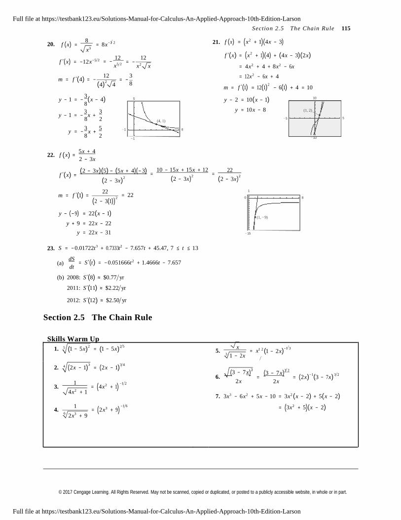
© 2017 Cengage Learning. All Rights Reserved. May not be scanned, copied or duplicated, or posted to a publicly accessible website, in whole or in part.
= −
x +
−1 3 2
8 2
Section 2.5 The C hain Ru le 115
20. f (x) = 8
= 8x−3 2
x3
21. f (x) = (x2 + 1)(4x − 3)
f ′(x) = (x2 + 1)(4) + (4x − 3)(2x)
f ′(x) = −12x−5 2 12 12
= − x5 2 x2 x
12 3 = 4x2 + 4 + 8x2 − 6 x
= 12 x2 − 6 x + 4m = f ′(4) = − = −
(4)2
4 8
m = f ′(1) = 12(1)2
− 6(1) + 4 = 10
y − 1 = − 3(x − 4)
8
y − 1 = − 3
x + 3
8 2
5
(4, 1)
y − 2 = 10(x − 1)
y = 10 x − 8
− 5
10
(1, 2)
5
3 5 − 1 8
y = − − 1
− 10
22. f (x) = 5x + 4 2 − 3x
f ′(x) = (2 − 3x)(5) − (5x + 4)(− 3)
(2 − 3x)2
22
= 10 − 15x + 15x + 12
(2 − 3x)2
= 22
(2 − 3x)2
1
m = f ′(1) = (2 − 3(1))
2
= 22 0 8
y − (−9) = 22(x − 1)
y + 9 = 22 x − 22
y = 22 x − 31
− 15
(1, − 9)
23. S = − 0.01722t 3 + 0.7333t 2 − 7.657t + 45.47, 7 ≤ t ≤ 13
(a)
dS = S ′(t ) = − 0.051666t 2 + 1.4666t − 7.657
dt
(b) 2008: S ′(8) ≈ $0.77 yr
2011: S ′(11) ≈ $2.22 yr
2012: S ′(12) ≈ $2.50 yr
Section 2.5 The Chain Rule
Skills Warm Up
1. 5 (1 − 5x)2
= (1 − 5x)2 5 x 1 2
−1 3
2. 4 (2 x − 1)
3
= (2 x − 1)
3 4
5. = x 3 1 − 2x
(1 − 2x)
3. 1
4x2 + 1
= (4x2
+ 1)
−1 2
( 3 − 7 x)3
6. 2 x
(3 − 7 x)3 2
= = (2 x) (3 − 7 x) 2 x
4. 1
6 2x3 + 9
= (2 x3
+ 9)
−1 6
7. 3x3 − 6x2 + 5x − 10 = 3x2 (x − 2) + 5(x − 2)
= (3x2 + 5)(x − 2)
Full file at https://testbank123.eu/Solutions-Manual-for-Calculus-An-Applied-Approach-10th-Edition-Larson
Full file at https://testbank123.eu/Solutions-Manual-for-Calculus-An-Applied-Approach-10th-Edition-Larson
© 2017 Cengage Learning. All Rights Reserved. May not be scanned, copied or duplicated, or posted to a publicly accessible website, in whole or in part.
2 3
−1 3
3
2
2
2 1 2
3
4 ( ) ( )
3
2
116 Chapte r 2 Dif ferentiat i on
Skills Warm Up —continued—
8. 5x x − x − 5 x + 1 = x(5 x − 1) − 1(5 x − 1) 10. − x5 + 6 x3 + 7 x2 − 42 = − x3 (x2 − 6) + 7(x2 − 6)
2
2 2
= (x − 1)(5
3
2 2
x − 1)
2
= (− x3 + 7)(x2 − 6)
= − (x3 − 7)(x2 − 6)
9. 4(x + 1) − x(x + 1) = (x + 1) 4 − x(x + 1)
2 2
3= (x + 1) (4 − x − x)
y = f (g (x)) u = g (x) y = f (u)
11. y = (5x4 − 2 x)
1. y = (6x − 5)4
2
u = 6x − 5
3
2
y = u 4
3
y′ = 2
(5x4
3
2
− 2 x) (20 x3 − 2)
−1 3 2. y = (x − 2 x + 3) u = x − 2 x + 3 y = u y′ = (5x4 − 2 x) (2)(10 x3 − 1) 3
3. y =
4. y =
5x − 2
3 9 − x2
u = 5x − 2
u = 9 − x2
y = u
y = 3 u
y′ = 4
(5x4 − 2 x)−1 3
(10x3 − 1)
4(10 x3 − 1) 40x3 − 4′ = =
y 4
1 3 3 x4 x5. y = (3x + 1)−1
u = 3x + 1 y = u −1
3(5x − 2x) 3 5 − 2
6. y = (x2 − 3)
−1 2
u = x2 − 3 y = u −1 2
12. y = (x 3 + 2 x2 )−1
3 2 − 2
2
7. y = (4x + 7)2
y′ = 2(4x + 7)1 (4)
y′ = (−1)(x
3x2
y′ = −
+ 2 x ) (3x
+ 4 x
+ 4x)
y′ = 8(4x + 7)
= 32x + 56
(x3 + 2x2 )2
f x = 2
= 2 1 − x3 −1
; (c) General Power Rule
8. y = (3x2
− 2) 13. ( )
1 − x3 ( )
y′ = 3(3x2 − 2) (6 x)
14. f (x) = 7
(1 − x)3
= 7(1 − x)−3
; (c) General Power Rule
y′ = 18x(3x2 − 2)
15.
f (x) =
3
82 ; (b) Constant Rule
9. y = 3 − x 2 = (3 − x2 )1 2
16.
f (x) = 3 x2
= x2 3 ; (a) Simple Power Rule
y′ = 1 (3 − x2 )
−1 2
(− 2x)
2 −1 2
x
17.
f (x) =
x2 + 9
; (d) Quotient Ruley′ = − x(3 − x ) = −
(3 − x ) x3 + 4x2 − 6
1 2
y′ = − x 18. f (x) =
x ; (d) Quotient Rule
3 − x2
x + 2 x − 5
y′ = 3 2x − 7 2
2
= 6 2x − 7 2
10. y = 4 4 6x + 5 = 4(6x + 5)1 4
19. ( ) ( ) ( )
1 −5 4
y′ = 4 6x + 5 6
20.
y = (3 − 5x)4
3 3
y′ = 6(6x + 5)−5 4
= 6
(6x + 5)5 4
21.
y′ = 4(3 − 5x) (−5) = − 20(3 − 5x)
h′(x) = 2(6x − x3 )(6 − 3x2 ) = 6x(6 − x2 )(2 − x2 )
Full file at https://testbank123.eu/Solutions-Manual-for-Calculus-An-Applied-Approach-10th-Edition-Larson
Full file at https://testbank123.eu/Solutions-Manual-for-Calculus-An-Applied-Approach-10th-Edition-Larson
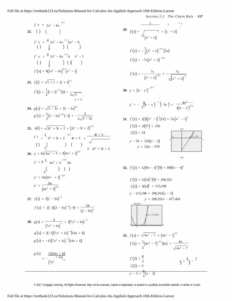
© 2017 Cengage Learning. All Rights Reserved. May not be scanned, copied or duplicated, or posted to a publicly accessible website, in whole or in part.
1 3
−
2
)
−
3
1 2
7
7 3
2
)
5
6
Section 2.5 The C h ain Ru le 117
f x = 4 3
2 x3 − 6x 1 2
− 7 2
22. ( ) ( ) 29.
f (x) = = (x + 11)
f ′ x
= 4
2x3 − 6x 1 3
6x2 − 6
(x2 + 11)
( ) ( ) ( ) 3
f ′(x) = −
7 (x2 + 11)−9 2
(2x)
f ′ x
= 4
2x3 − 6x 1 3
6
x2 − 1 2
( ) ( ) ( )( ) 3
f ′(x) = − 7 x(x2 + 11) −9 2
f ′(x) = 8(2x3 − 6x) (x2
− 1) f ′(x) = −
7 x
2
7 x 9 2
= − 9
2
23. f (t ) = t + 1 = (t + 1)1 2
(x + 11) (x + 11)
4 3
y = 4 − x3
f ′(t) = 1 (t + 1)
−1 2 (1) =
2 2 1
t + 1
30. ( )
4
3 −7 3
2
4 x2
24.
g (x) =
5 − 3x
= (5 − 3x)1 2
y′ = −
(4 − x ) (− 3x ) = 3
3(4 − x2 )
g′(x) = 1 (5 − 3x)
−1 2 (−3) = −
3 2 2 5 − 3x
31.
f ′(x) = 2(3)(x2
− 1) (2 x) = 12x(x2
− 1)
25.
s(t) =
2t 2 + 5t + 2 = (2t 2
1 2
+ 5t + 2 f ′(2) = 24(32 ) = 216
200
s′ t
1 −1 2
= 2t 2 + 5t + 2 4t + 5 4t + 5
=
f (2) = 54 (2, 54)
( ) ( ) ( ) 2 2 2t 2 + 5t + 2
y − 54 = 216(x − 2) − 2 4
y = 216 x − 378
3 2 2 1 3
26. y = 9 4x
y′ = 9 1
+ 3 = 9(4 x
2 3
4x2 + 3 8x
+ 3) − 400
( ) ( )
32. f ′(x) = 12(9x − 4)3 (9) = 108(9 x − 4)
3
y′ = 24 x(4x2 + 3)
− 2 3
f ′(2) = 12(14)3 (9) = 296,352
y′ = 24 x
4
(4 x2
2 3
+ 3 f (2) = 3(14) = 115,248
27.
f (x) = 2(2 − 9x)−3
y − 115,248 = 296,352(x − 2)
y = 296,352x − 477,456
f ′(x) = 2(− 3)(2 − 9 x)− 4
(− 9) = 54
(2 − 9 x)4
200,000
(2, 115,248)
g x = 3
= 3 7 x2 + 6x −5
28. ( ) ( ) (7 x2 + 6x)
2 −6
− 1 5
0
g′(x) = 3(−5)(7 x
2
+ 6x) (14 x + 6) − 6
33. f (x) =
4x2 − 7 = (4 x2 − 7)g′(x) = −15(7 x + 6x) (14 x + 6) f ′(x) =
1 (4 x2 − 7)
−1 2
(8x) = 4 x
2 4x2 − 7
g′(x) 15(14 x + 6)= −
(7 x2
+ 6 x) f ′(2) = 8
3
f (2) = 3
y − 3 = 8(x − 2)
3
y = 8
x − 7
3 3
Full file at https://testbank123.eu/Solutions-Manual-for-Calculus-An-Applied-Approach-10th-Edition-Larson
Full file at https://testbank123.eu/Solutions-Manual-for-Calculus-An-Applied-Approach-10th-Edition-Larson
© 2017 Cengage Learning. All Rights Reserved. May not be scanned, copied or duplicated, or posted to a publicly accessible website, in whole or in part.
10
(
2
,
3
)
− 1 4
− 4
Full file at https://testbank123.eu/Solutions-Manual-for-Calculus-An-Applied-Approach-10th-Edition-Larson
Full file at https://testbank123.eu/Solutions-Manual-for-Calculus-An-Applied-Approach-10th-Edition-Larson
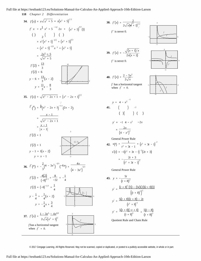
© 2017 Cengage Learning. All Rights Reserved. May not be scanned, copied or duplicated, or posted to a publicly accessible website, in whole or in part.
)
)
−
2 − 2
−
−2
2
3
2 2
x + 4
( 3
(
−1
4
5 3
1
2
118 Chapte r 2 Differentiat i on
34. f (x) = x x 1 2
2 + 5 = x x2 + 5 38. f ′(x) =
2
f ′ x
= x1
x2 + 5 −1 2
2x +
1 2
x2 + 5 1
2 x (x + 1)3 2
( ) ( ) ( ) 2
( ) ( ) f ′ is never 0. f
f ′ − 1 3
= x2 (x2 + 5)
−1 2 1 2
+ x2 + 5 −1
= (x2 + 5)
−1 2
x 2 + (x2
+ 5) 4
2 x2 + 5 =
x2 + 5
39.
(x + 1) x f ′(x) = −
2x(x + 1) f
f ′ is never 0. − 5 4
f ′(2) = 13 10
3
f (2) = 6
f ′
− 3
2 − 5x2 4
y − 6 = 13
(x − 2) 3 − 1
40.
4
f ′(x) = 2 x
y = 13
x − 8 f has a horizontal tangent −1 4
3 3
2 2
1 2
when f ′ = 0. f
f ′
− 4
35. f (x) = x − 2x + 1 = (x − 2x + 1) 1
y = 4 − x2
f ′ x = 1
x2 − 2 x + 1 −1 2
2x − 2 41. ( )( ) ( ) ( ) x − 1
=
( )( ) ( )
x2 − 2x + 1
x − 1 =
x − 1 3
f ′(2) = 1
y′ = −1 4 − x2
= 2 x
(4 − x2 )2
General Power Rule
− 2x
(2, 1)
s t = 1
=
1
t 2 + 3t − 1f (2) = 1 − 2 42. ( ) t 2 + 3t − 1
( )
y − 1 = 1(x − 2)
y = x − 1 − 3
s′(t ) = −1(t 2 + 3t − 1) (2t + 3)
= − 2t + 3
f ′ x
2 4 − 3x2
−5 3
−6 x
4 x
=
(t 2 + 3t − 1)36. ( ) = − ( ) ( )
(4 − 3x2 ) General Power Rule
4(2) 8 1 f ′(2) = = = −
43.
y = − 5t
(−8)5 3
−32 4 (t + 8)2
f (2) = (−8)−2 3
= 1
4
2
(2 , 1
y′ = (t + 8)
2 (5) − (5t )(2)(t + 8)(1)
((t + 8) )y −
1 4
= − (x − 2) − 2 4
4 4 y′ = 5(t + 8)(t + 8) − 2t
1 3 y = −
4 4 − 2
1 − 3x2 − 4 x3 2 2
(t 2 + 8) 5(t + 8)(− t + 8)
y′ = (t + 8)
4
5(t − 8) =
(t + 8)3
37. f ′(x) = 2 x (x2 + 1) f
Quotient Rule and Chain Rule
f has a horizontal tangent − 1 5
when f ′ = 0. f ′
− 2
Full file at https://testbank123.eu/Solutions-Manual-for-Calculus-An-Applied-Approach-10th-Edition-Larson
Full file at https://testbank123.eu/Solutions-Manual-for-Calculus-An-Applied-Approach-10th-Edition-Larson

© 2017 Cengage Learning. All Rights Reserved. May not be scanned, copied or duplicated, or posted to a publicly accessible website, in whole or in part.
−
) )
)
3
Section 2.5 The C hain Ru le 119
2
f x = 3x x3 − 4 50. f (x) = x3 (x − 4)2
44. ( ) ( )
3 −3
2 3 − 2
= x3 (x2 − 8x + 16)f ′(x) = 3x(− 2)(x − 4) (3x )
+ (x − 4) (3) = x5 − 8x4 + 16 x3
= −18x3 (x3
−3
− 4 + 3(x3
− 2
− 4 f ′(x) = 5x4 − 32 x3 + 48x2
= − 3(x3 −3
− 4 6x 3 − (x3
− 4) = x2 (5x2 − 32 x + 48)
− 3(5x3 + 4)
= x2 (5x − 12)(x − 4)=
(x3 − 4)
Simple Power Rule
Product Rule and Chain Rule
51.
y = x 2 x + 3 = x(2x + 3)1 2
45. f (x) = (2x − 1)(9 − 3x2 ) y′ = x
1 (2 x + 3)
−1 2 (2)
+ (2 x + 3)
1 2
2
f ′(x) = (2 x − 1)(− 6x) + (9 − 3x2 )(2)
= (2x + 3)−1 2
x + (2x + 3)
= −12x2 + 6 x + 18 − 6 x2
= 18 + 6x − 18x2
3( x + 1) =
2x + 3
= − 6(3x2 − 2 x − 3) Product and General Power Rule
Product Rule and Simple Power Rule 52.
y = 2t t + 6
= 2t(t + 6)1 2
46. y = (7 x + 4)(x3 − 2x2 ) y′ = 2t 1 (t + 6)
−1 2 (1)
+ (t + 6)
1 2 (2) 2
y′ = (7 x + 4)(3x2 − 4x) + (x3 − 2x2 )(7)
= 21x3 − 16 x2 − 16x + 7 x3 − 14x2
= t(t + 6)−1 2
( )−1 2
+ 2(t + 6)1 2
( )
= 28x3 − 30x2 − 16x = t + 6 t + 2 t + 6
−1 2
Product Rule and Simple Power Rule = (t + 6) (3t + 12)
47.
y = 1
= (x + 2)−1 2
= 3t + 12
= t + 6
3(t + 4) t + 6
x + 2
y′ 1 (x
2)
−3 2
1
Product and General Power Rule
= − + = − 2 2(x + 2)
3 2
53.
y = t 2
t − 2
= t 2 (t − 2)1 2
General Power Rule
48. g (x) = 3
= 3(x3 − 1)−1 3
y′ = t 2 1
2
1
(t − 2)−1 2
(1) + 2t(t − 2)
1 2
−1 2 23 x3 − 1 = (t − 2)
2 t + 4t(t − 2)
1 3
−4 3
2
3x 2
2g′(x) = 3 − (x − 1) (3x ) = −
4 3 t + 4t (t − 2)
= 3 (x3 − 1) 2 t − 2
General Power Rule =
t (5t − 8)
49.
f (x) = x(3x − 9)3
2 t − 2
f ′(x) = x(3)(3x − 9)2 (3) + (3x − 9)
3 (1)
= (3x − 9)2 9x + (3x − 9)
= 9(x − 3)2 (12 x − 9)
= 27(x − 3)2 (4 x − 3)
Product and General Power Rule
Product and General Power Rule
Full file at https://testbank123.eu/Solutions-Manual-for-Calculus-An-Applied-Approach-10th-Edition-Larson
Full file at https://testbank123.eu/Solutions-Manual-for-Calculus-An-Applied-Approach-10th-Edition-Larson
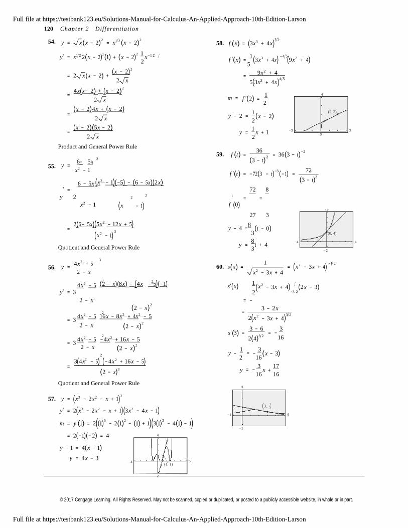
© 2017 Cengage Learning. All Rights Reserved. May not be scanned, copied or duplicated, or posted to a publicly accessible website, in whole or in part.
1 5
=
2
y = 6 5x
3
2 2
( −3 2
2
)
2
)
3
2
− 1
120 Chapte r 2 Dif ferentiat i on
54. y = x (x − 2)2 = x1 2 (x − 2)
2
58. f (x) = (3x3 + 4x)
y′ = x1 2 2(x − 2)1 (1) + (x − 2)
2 1 x−1 2
1 − 4 5
2
f ′(x) = (3x3 + 4x) (9x2 + 4) 5
2 2
= 2 x (x − 2) + ( x − 2) 9 x + 4
=2 x 5(3x3
4 5
+ 4x
4 x( x− 2) + ( x − 2)2
= 1 4
2 x m = f ′(2) = 2
( x − 2)4 x + ( x − 2)
1 (2, 2)
2 x y − 2 = (x − 2) 2
= ( x − 2)(5x − 2)
y = 1
x + 1 − 3 3
2 x 2 0
Product and General Power Rule
59.
f (t) = 36
= 36(3 − t )−2
55.
2
− x2 − 1
6 − 5x ( x2 − 1)(−5) − (6 − 5x)(2 x)
′ =
(3 − t )
f ′(t) = −72(3 − t )−3
(−1) =
72 8
72
(3 − t )3
y 2
x2 − 1
2 2 ′ = =
(x
− 1)
f (0) 12
27 3
2(6− 5x)(5x2 − 12 x + 5) 8=
(x2
− 1) y − 4 = (t − 0)
3 (0, 4)
Quotient and General Power Rule
4x2 − 5
y = 8
t + 4 3
1
− 4 4
− 2
−1 2
56. y = 60. s(x) = = (x2 − 3x + 4) 2 − x x2 − 3x + 4
4 x2 − 5 (2 − x)(8 x) − (4 x − 5)(−1)
y′ = 3
s′(x) 1
x2
2 − 3x + 4) (2 x − 3)
2 − x = −
(2 − x)2
4 x2 − 5 16 x − 8x2 + 4 x2 − 5= 3
=
2(x2
3 − 2x 3 2
− 3x + 4
2 − x (2 − x)2
s′ 3
= 3 − 6
= − 3
4 x2 − 5 − 4 x2 + 16 x − 5= 3
( ) 2(4)
3 2 16
2 − x
2
2
(2 − x)
2
2
y − 1
= − 3
2 16
(x − 3)3(4x − 5) (− 4 x + 16 x − 5)
= (2 − x)
3 y 3
x + 17 = −
Quotient and General Power Rule
16 16
3
57. y = (x
3 − 2 x2
− x + 1)
(3 , 1
y′ = 2(x3 − 2 x2 − x + 1)(3x2 − 4x − 1) 2
− 1 5
m = y′(1) = 2((1)3 − 2(1)
2 − (1) + 1)(3(1)
2 − 4(1) − 1)
= 2(−1)(− 2) = 4
y − 1 = 4(x − 1)
y = 4x − 3 − 4
4
5
(1, 1)
− 2
Full file at https://testbank123.eu/Solutions-Manual-for-Calculus-An-Applied-Approach-10th-Edition-Larson
Full file at https://testbank123.eu/Solutions-Manual-for-Calculus-An-Applied-Approach-10th-Edition-Larson
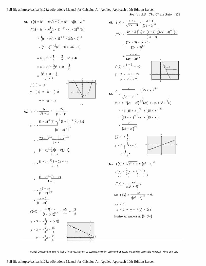
© 2017 Cengage Learning. All Rights Reserved. May not be scanned, copied or duplicated, or posted to a publicly accessible website, in whole or in part.
2
2 2
−
3
3 2
x +
1
5
)
8 8
Section 2.5 The C hain Ru le 121
61.
f (t) = (t 2 − 9)
t + 2
= (t 2 − 9)(t + 2)1 2
63.
f (x) x + 1 x + 1
f ′(t) = (t 2 − 9)1 (t + 2)
−1 2 + (t + 2)
1 2 (2t)
= = 2 x − 3 (2x − 3)
1 2
2
2x − 3 1 2
1 − x + 1 1 2 x − 3
−1 2 2
= 1 (t 2 − 9)(t + 2)
−1 2 + 2t(t + 2)
1 2
= (t + 2)−1 2 1 (t 2 − 9) + 2t(t + 2)
f ′(x) =
=
( ) ( ) ( )( 2 )( ) ( ) (2x − 3)
(2 x − 3) − ( x + 1)
(2x − 3)3 2
2
= (t + 2)−1 2 1
t 2 − 9
+ 2t 2 + 4t x − 4
= 3 2
2 2 (2x − 3) 6
= (t + 2)−1 2 5
t 2 + 4t − 9
5 t 2 + 4t − 9
= 2 2
t + 2 2
f ′(2) = 1 − 3
= −2 1
y − 3 = −2(x − 2)
y = −2x + 7
(2, 3)
− 4 8
− 2
f ′(−1) = −6 − 4
4
y x
1 2
x x2
y − (−8) = −6t − (−1) (− 1, − 8) 64. = =
25 + x2
(25 + )
y = −6t − 14 y′ = x− 1 (25 + x2 )
−3 2
(2 x) + (25 + x2 )−1 2
(1) − 16 2
2 2 −3 2
2
−1 2
62. y = − 2 x 2 x
= − 1 2
= − x (25 + x ) + (25 + x )1 − x (1 − x)
= (25 + x2 )
−3 2
− x2 + (25 + x2 )(1 − x)
1 2 (2) −
1 (1 − x)
−1 2 (−1)(2 x)
y′ = − 2
1 2 2
= 25
2 3 2
((1 − x) )
y′ 0
(25 + x )
= 1
2(1 − x)1 2
+ x(1 − x)−1 2 ( )
= − 1 − x
y − 0 = 1 (x − 0) − 3 3
(1 − x)−1 2(2(1 − x) + x)
5
= − 1 1 − x y = x
−1
(1 − x)−1 2
(2 − 2 x + x)
5
3 2 2
1 3 = − 65. f (x) = x + 4 = (x + 4)
1 − x f ′ x
= 1
x2 + 4 − 2 3
2 x
(1 − x)−1 2
(2 − x) = −
( ) ( ) ( )
1 − x f ′(x) =
2 x
(2 − x) = −
3(x2
2 3
+ 4
(1 − x)
Set f ′(x) = 2 x 2 3
= 0.
x − 2 =
(1 − x)3 2
2 x = 0
3(x2 + 4)
y′(−3) = (− 3) − 2
= − 5
= − 5 x = 0 → y = f (0) = 3 4
(1 − (−3))3 2
y − 3 = − 5(x − (− 3))
8
y − 3 = − 5
x − 15
8 8
43 2 8
6
(−3, 3)
Horizontal tangent at: (0, 3 4 )
5 9 y = − −7 1
−1
Full file at https://testbank123.eu/Solutions-Manual-for-Calculus-An-Applied-Approach-10th-Edition-Larson
Full file at https://testbank123.eu/Solutions-Manual-for-Calculus-An-Applied-Approach-10th-Edition-Larson

© 2017 Cengage Learning. All Rights Reserved. May not be scanned, copied or duplicated, or posted to a publicly accessible website, in whole or in part.
)
2
2
( )
2
f =
501
59
501
59
501
59
1 2
122 Chapte r 2 Dif ferentiat i on
66. f (x) = 5x2 + x − 3 = (5x2
1 2
+ x − 3
68. f (x) = 5x
= 3x − 2
5x
(3x − 2)1 2
f ′ x
= 1
5x2 + x − 3 −1 2
10x + 1
( ) ( ) ( )
(3x − 2)1 2
(5) − 5x 1
(3x − 2)−1 2
(3)
f ′(x) = 10 x + 1 1 2
f ′(x) = 2
1 2
2(5x2 + x − 3) (3x − 2)
Set
f ′(x) =
10 x + 1
1 2 = 0.
2(5x2 + x − 3)
f ′(x) =
5(3x − 2)1 2
− 15
x(3x − 2)−1 2
2 (2x + 1)
10x + 1 = 0
x 1
y f
1 61
5 (3x − 2)
−1 2 2(3 − x2) − 3x
f ′(x) = 2 = − → =
10 −
10 = −
20
f ′ x
(2x − 1)
5(3x − 4) =
Because − 61
20
is not a real number, there is no point ( )
2(3x − 2)3 2
67.
of horizontal tangency.
f (x) = x
= x
Set f ′(x) = 5(3x − 4)
= 0.
2(3x − 2)3 2
2 x − 1 (2x − 1) 5(3x − 4) = 0
f ′(x) =
(2x − 1)1 2
(1) − x 1
(2x − 1)−1 2
(2)
1 2 2
2 x + 1
3x − 4 = 0
x = 4
→ y = 3
4 3
20
3 2
1 2 −1 2 4 10
f ′(x) = (2 x − 1) − x(2 x − 1)
(2 x + 1) −1 2
Horizontal tangent at: 3
, 3 2
59 59
f ′(x) = (2 x − 1) (2 x − 1) − x
69. A′ = 1000(60) 1 + r
1
= 5000 1 + r
(2x − 1)
12
12
12
f ′(x) = x − 1
(2x − 1)3 2
(a)
A′(0.08) =
+
0.08
12
Set
f ′(x) = x − 1
3 2 = 0.
≈ $74.00 per percentage point
x − 1 = 0
(2 x − 1) (b) A′(0.10) =
+
0.10
12
x = 1 → y = f (1) = 1
= 1 ≈ $81.59 per percentage point
1
Horizontal tangent at: (1, 1)
(c) A′(0.12) =
+ 0.12
12
≈ $89.94 per percentage point
Full file at https://testbank123.eu/Solutions-Manual-for-Calculus-An-Applied-Approach-10th-Edition-Larson
Full file at https://testbank123.eu/Solutions-Manual-for-Calculus-An-Applied-Approach-10th-Edition-Larson
© 2017 Cengage Learning. All Rights Reserved. May not be scanned, copied or duplicated, or posted to a publicly accessible website, in whole or in part.
2
2
2
3
dt
Section 2.6 Highe r- Orde r Derivative s 123
70. N = 4001 − 3(t + 2) − 2
71. V = k
t + 1
dN
2 −3
When t = 0, V
= 10,000.= N ′(t) = 400(− 3)(− 2)(t + 2) (2t)
dt
= 4800t
(t 2 + 2)
10,000 = k
k 0 + 1
10,000
= 10,000
(a)
N ′(0) = 0 bacteria day
V = t + 1
−1 2
(b) N ′(1) ≈ 177.8 bacteria day V = 10,000(t + 1)
dV 5000 t
1
−3 2 1 5000
(c) N ′(2) ≈ 44.4 bacteria day = − ( dt
+ ) ( ) = − 3 2
(t + 1)(d) N ′(3) ≈ 10.8 bacteria day
When t = 1,
(e) N ′(4) ≈ 3.3 bacteria day dV 5000 2500 $1767.77 per year.= −
3 2 = − ≈ −
(f ) The rate of change of the population is decreasing as
time passes.
dt (2)
dV
2
5000When t = 3,
dt = − = −$625.00 per year.
(4)3 2
72. (a) From the graph, the tangent line at t = 4 is steeper than the tangent line at t = 1. So, the rate of change after
4 hours is greater.
(b) The cost function is a composite function of x units, which is a function of the number of hours, which is not a linear function.
4 3 2 1 2
73. (a) r = (0.3017t − 9.657t + 97.35t − 266.8t − 242)dr
= r′ t
= 1
0.3017t 4 − 9.657t 3 + 97.35t 2 − 266.8t − 242 −1 2
⋅
1.2068t 3 − 28.971t 2 + 194.7t − 266.8( ) ( ) ( )
(b)
=
Chain Rule
4
1.2068t 3 − 28.971t 2 + 194.7t − 266.8
2 0.3017t 4 − 9.657t 3 + 97.35t 2 − 266.8t − 242
8 13
− 2
(c) The rate of change appears to be the greatest when t = 8 or 2008.
The rate of change appears to be the least when t ≈ 9.60, or 2009, and when t ≈ 12.57, or 2012.
Section 2.6 Higher-Order Derivatives
Skills Warm Up
1. −16t 2 + 292 = 0 2. −16t 2 + 88t = 0
−16t 2
t 2
= − 292
= 73 4
−8t(2t − 11) = 0
−8t = 0 → t = 0
2t − 11 = 0 → t = 11
t = ± 73 2
Full file at https://testbank123.eu/Solutions-Manual-for-Calculus-An-Applied-Approach-10th-Edition-Larson
Full file at https://testbank123.eu/Solutions-Manual-for-Calculus-An-Applied-Approach-10th-Edition-Larson
© 2017 Cengage Learning. All Rights Reserved. May not be scanned, copied or duplicated, or posted to a publicly accessible website, in whole or in part.
2
3
4
2
124 Chapte r 2 Dif ferentiat i on
Skills Warm Up —continued—
3. −16t 2 + 128t + 320 = 0
−16(t 2 − 8t − 20) = 0
−16(t − 10)(t + 2) = 0
t − 10 = 0 → t = 10
t + 2 = 0 → t = −2
4. −16t 2 + 9t + 1440 = 0
7. y =
dy
= dx
=
x 2
2x + 7
(2 x + 7)(2 x) − ( x 2 )(2)
(2x + 7)2
4x2 + 14 x − 2 x2
(2x + 7)2
2x2 + 14 x−9 ±
t = 92 − 4(−16)(1440)
2(−16) =
(2 x + 7)2
= −9 ± 92241
−32
2 x( x+ 7) =
(2 x + 7)2
= 9 ± 3 10249
32
8. y =
x2 + 3x 2
t ≈ − 9.21 and t ≈ 9.77 2x − 5
5. y = x2 (2 x + 7) dy (2 x2 − 5)(2 x + 3) − ( x2 + 3x)(4 x)
= dx (2x2 − 5)
dy = x2 (2) + 2x(2 x + 7)
dx 4 x3 + 6 x2 − 10 x − 15 − 4 x3 − 12 x2
= 2
= 2 x2 + 4x2 + 14x (2x2 − 5)
= 6x2 + 14x −6 x 2 − 10 x − 15 =
6. y = (x2 + 3x)(2x2 − 5) (2x2
− 5)
dy = (x2 + 3x)(4 x) + (2x + 3)(2x2 − 5)
9. ( )
f x = x2 − 4
dx
= 4 x3 + 12x2 + 4x3 − 10x + 6 x2 − 15
= 8x3 + 18x2 − 10 x − 15
Domain: (−∞, ∞)
Range: [− 4, ∞)
10. f (x) = x − 7
Domain: [7, ∞)
Range: [0, ∞)
1. f (x) = 9 − 2x
f ′(x) = −2
f ′′(x) = 0
2. f (x) = 4x + 15
f ′(x) = 4
f ′′(x) = 0
4. f (x) = 3x2 + 4x f
′(x) = 6 x + 4
f ′′(x) = 6
5. g (t) = 1 t 3 − 4t
2 + 2t
g′(t) = t 2 − 8t + 2
g′′(t) = 2t − 8
3. f (x) = x2 + 7 x − 4 6. f (x) = − 5 x 4 + 3x2 − 6 x
f ′(x) = 2x + 7
f ′′(x) = 2
f ′(x) = − 5x3 + 6x − 6
f ′′(x) = −15x2 + 6
Full file at https://testbank123.eu/Solutions-Manual-for-Calculus-An-Applied-Approach-10th-Edition-Larson
Full file at https://testbank123.eu/Solutions-Manual-for-Calculus-An-Applied-Approach-10th-Edition-Larson
© 2017 Cengage Learning. All Rights Reserved. May not be scanned, copied or duplicated, or posted to a publicly accessible website, in whole or in part.
= −
4
3
= −
3
3
2
Section 2.6 Highe r- Orde r Derivative s 125
7. f (t ) = 2
= 2t −3 13. f (x) = x5 − 3x4
t ( ) 4 3
f ′(t ) = − 6t − 4 f ′ x = 5x − 12x
f ′′(t) = 24t −5
= 24
f ′′(x) = 20x3 − 36x2
2
t 5 f ′′′(x) = 60x − 72x
8. g (t ) = 5
= 6t 4
5 t − 4
6
14.
f (x) = x4 − 2 x3
g′(t ) 10
t −5 f ′(x) = 4 x
3 − 6x2
3
g′′(t ) = 50
t − 6
= 50
f ′′(x) = 12x2 − 12x
f ′′′(x) = 24 x − 12 = 12(2x − 1)3 3t 6
9. f (x) = 3(2 − x2 )3
f ′(x) = 9(2 − x ) (−2x) = −18x(2 − x )
15.
f (x) = 5x(x + 4)3
= 5x(x3 + 12x2 + 48x + 64)2 2
2 2
f ′′(x) = (−18x)2(2 − x2 )(−2x) + (2 − x2 )2
(−18)
= 18(2 − x2 )4x2 − (2 − x2 )
= 5x4 + 60x3 + 240x2 + 320 x
f ′(x) = 20x3 + 180x2 + 480 x + 320
f ′′(x) = 60x2 + 360x + 480
= 18(2 − x2 )(5x2 − 2) f ′′′(x)
120x
360= +
10. y = 4(x2 + 5x)
2 2
16. f (x) = (x3 − 6)
y′ = 4(3)(x + 5x) (2x + 5) f ′(x) = 4(x3 − 6) (3x2 )= (24x + 60)(x4 + 10x3 + 25x2 ) = 24x5 + 300x4 + 1200x3 + 1500x2
y′′ = 120x4 + 1200x3 + 3600x2 + 3000 x
= 12x11 − 216 x8 + 1296x5 − 2592x2
f ′′(x) = 132x10 − 1728x7 + 6480x4 − 5184 x
f ′′′(x) = 1320x9 − 12,096x6 + 25,920x3 − 5184
11. f (x) = x + 1 17. f ( x) =
3 =
3 x− 4
x − 1
f ′(x) = ( x − 1)(1)− ( x + 1)(1)
f ′( x)
8x4 8
3 x−5
(x − 1)2
= −
15= −
2 = −2( x − 1)
−2 f ′′( x) = x−6
(x − 1)2
f ′′′ x
2
= − 45x−7 45
12.
f ′′(x) = 4(x − 1)−3
(1) = 4
(x − 1)3
g (x) = 1 − 4 x
x − 3
18.
( ) = − x7
f (x) = − 2
25x5
2
g′( x) = ( x − 3)(− 4) − (1 − 4 x)(1)
f (x) = − 25
x−5
( x − 3)2
f ′(x) = 2
x− 6
5
= − 4 x + 12 − 1 + 4 x
(x − 3)2
f ′′(x) 12 5
x− 7
= 11
= 11(x − 3)− 2
( x − 3)2
g′′( x) = − 22(x − 3)−3
(1) = − 22
f ′′′(x) = 84
x−8
5 =
84 5x8
(x − 3)3
Full file at https://testbank123.eu/Solutions-Manual-for-Calculus-An-Applied-Approach-10th-Edition-Larson
Full file at https://testbank123.eu/Solutions-Manual-for-Calculus-An-Applied-Approach-10th-Edition-Larson
© 2017 Cengage Learning. All Rights Reserved. May not be scanned, copied or duplicated, or posted to a publicly accessible website, in whole or in part.
= −
f ′′
4
126 Chapte r 2 Dif ferentiat i o n
19.
20.
g (t) = 5t 4 + 10t 2 + 3
g′(t) = 20t 3 + 20t
g′′(t) = 60t 2 + 20
g′′(2) = 60(4) + 20 = 260
f (x) = 9 − x2
26. 27.
f ′′(x) = 20x3 − 36x2
f ′′′(x) = 60x2 − 72x = 12x(5x − 6)
f ′′′(x) = 4x− 4
f (4) (x) = −16x−5
f ′(x) = −2x
f ′′(x) = −2
f (5) (x) = 80x− 6 =
80 x6
1 2
f ′′(− 5 ) = −2 28. f ′′(x) = 4 x − 2 = 4(x − 2)
f ′′′(x) = 4 1 (x − 2)−1 2 (1) = 2(x − 2)−1 2
21. f (x) =
4 − x
= (4 − x)1 2 2
f 4 x
= 2 − 1
x − 2 −3 2
1
= − x − 2
−3 2
f ′(x) 1 (4 − x)
−1 2
( ) ( ) ( ) ( ) ( )
= − 2
f 5 x
2
= 3
x − 2 −5 2
1
= 3
f ′′(x) 1 (4 − x)
−3 2
( ) ( ) ( ) ( ) = − 2 2(x − 2)5 2
f ′′′(x) 3
(4 − x)−5 2
= −3
= − 8 8(4 − x)
5 2
29. f (5) (x) = 2(x2 + 1)(2x)
3
f ′′′(−5) = −3 1 5 2
= − 648
= 4 x + 4x
22.
f (t) =
8(9)
2t + 3 = (2t + 3)1 2
30.
f (6) (x) = 12x2 + 4
f ′′′(x) = 4x + 7
f ′(t) = 1 (2t + 3)
−1 2 (2) = (2t + 3)
−1 2
2 f (4) (x) = 4
f (5) (x) = 0
f ′′(t) 1 (2t + 3)
−3 2 (2) = −(2t + 3)
−3 2
2
31.
f ′(x) = 3x2 − 18x + 27
f ′′′(t) = 3
(2t + 3)−5 2
(2) = 3
1 ′ = 2
2
3
32
(2t + 3)5 2
f ′′(x) = 6x − 18
f ′′(x) = 0 6x = 18
x = 3
f x =
3
x3 − 2x
= x9 − 6x7 + 12 x5 − 8x323. ( ) ( )
f ′(x) = 9x8 − 42x6 + 60x4 − 24x2
32.
f (x) = (x + 2)(x − 2)(x + 3)(x − 3)
= (x2 − 4)(x2 − 9) 4 2
f ′′(x) = 72x7 − 252x5 + 240x3 − 48x
f ′′(1) = 12
= x
f ′(x) = 4 x
− 13x
3 − 26x
+ 36
g x =
4
x2 + 3x = x8 + 12 x7 + 54 x6 + 108x5 + 81x4
f ′′(x) = 12x2 − 26
24. ( ) ( ) g′(x) = 8x7 + 84x6 + 324x5 + 540x4 + 324x3
f ′′(x) = 0 12 x2
= 26 13 78
g′′(x) = 56x6 + 504x5 + 1620x4 + 2160x3 + 972x2
g′′(−1) = −16
x = ± = ± 6 6
25. f ′( x) = 2x2
f ′′(x) = 4x
Full file at https://testbank123.eu/Solutions-Manual-for-Calculus-An-Applied-Approach-10th-Edition-Larson
Full file at https://testbank123.eu/Solutions-Manual-for-Calculus-An-Applied-Approach-10th-Edition-Larson
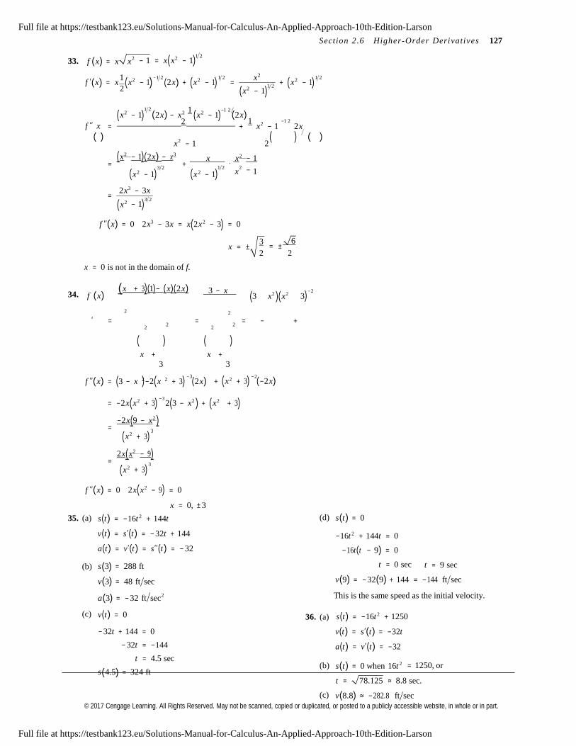
© 2017 Cengage Learning. All Rights Reserved. May not be scanned, copied or duplicated, or posted to a publicly accessible website, in whole or in part.
)
) 1 2
)
3
(
1 2
)
−2
−3
3
Section 2.6 Highe r- Orde r Derivative s 127
33. f (x) = x x 1 2 2 − 1 = x x2 − 1
1 −1 2 1 2 x2 1 2 f ′(x) = x (x2 − 1) (2 x) + (x2 − 1) = + (x2 − 1)
2 (x2 − 1
(x2 − 1) (2x)
− x2 1 (x2 − 1)
−1 2
(2x)f ′′ x
= 2 + 1
x2 − 1 −1 2
2x
( ) x2 − 1 2
( ) ( )
( x 2 − 1)(2 x) − x3 x x 2 − 1=
3 2 +
2 2 1 2
⋅ 2 −(x − 1) (x − 1) x 1
2x3 − 3x=
(x2
3 2
− 1
f ′′(x) = 0 2 x3 − 3x = x(2x2 − 3) = 0
x = ± 3
= ± 6
34.
x = 0 is not in the domain of f.
f (x) ( x + 3)(1)− ( x)(2 x)
3 − x
2 2
(3 x2 )(x2 3
2 2
′ = = = − + 2
2 2
2
( ) ( ) x + x +
3 3
2 2
−3
2
−2f ′′(x) = (3 − x )−2(x
+ 3) (2 x) + (x + 3) (−2 x)
= −2x(x2 + 3) 2(3 − x2 ) + (x2 + 3)
−2 x(9 − x2 )=
(x2 + 3)
2 x( x2 − 9)=
(x2 + 3)
f ′′(x) = 0 2 x(x2 − 9) = 0
x = 0, ± 3
35. (a)
(b)
s(t ) = −16t 2 + 144t
v(t ) = s′(t ) = − 32t + 144
a(t ) = v′(t ) = s′′(t ) = − 32
s(3) = 288 ft
(d) s(t) = 0
−16t 2 + 144t = 0
−16t(t − 9) = 0
t = 0 sec
t = 9 sec
(c)
v(3) = 48 ft sec
a(3) = − 32 ft sec2
v(t ) = 0
− 32t + 144 = 0
− 32t = −144
t = 4.5 sec
36. (a)
v(9) = − 32(9) + 144 = −144 ft sec
This is the same speed as the initial velocity.
s(t ) = −16t 2 + 1250
v(t ) = s′(t) = −32t
a(t ) = v′(t ) = −32
s(4.5) = 324 ft (b) s(t) = 0 when 16t 2 = 1250, or
t = 78.125 ≈ 8.8 sec.
(c) v(8.8) ≈ −282.8 ft sec
Full file at https://testbank123.eu/Solutions-Manual-for-Calculus-An-Applied-Approach-10th-Edition-Larson
Full file at https://testbank123.eu/Solutions-Manual-for-Calculus-An-Applied-Approach-10th-Edition-Larson
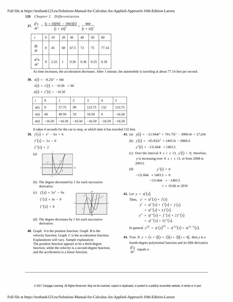
© 2017 Cengage Learning. All Rights Reserved. May not be scanned, copied or duplicated, or posted to a publicly accessible website, in whole or in part.
f
128 Chapte r 2 Dif ferentiat i on
37.
d2 s = (t + 10)(90) − (90t )(1)
= 900
dt 2
(t 10)2
(t 10)2
+ +
t 0 10 20 30 40 50 60
ds
dt
0
45
60
67.5
72
75
77.14
d 2 s
dt 2
9
2.25
1
0.56
0.36
0.25
0.18
38.
As time increases, the acceleration decreases. After 1 minute, the automobile is traveling at about 77.14 feet per second.
s(t ) = −8.25t 2 + 66t
v(t ) = s′(t ) = −16.50t + 66
a(t ) = s′′(t ) = −16.50
t 0 1 2 3 4 5
s(t) 0 57.75 99 123.75 132 123.75
v(t) 66 49.50 33 16.50 0 −16.50
a(t) −16.50 −16.50 −16.50 −16.50 −16.50 −16.50
It takes 4 seconds for the car to stop, at which time it has traveled 132 feet.
39. f (x) = x2 − 6x + 6
f ′(x) = 2x − 6
f ′′(x) = 2
41. (a)
(b)
y(t ) = − 21.944t 3 + 701.75t 2 − 6969.4t + 27,164
y′(t) = − 65.832t 2 + 1403.5t − 6969.4
y′′(t) = −131.664t + 1403.5
(a) 7 (c) Over the interval 8 ≤ t ≤ 13, y′(t) > 0; therefore,
f ″ f ′
− 5 10
f
− 3
(d)
y is increasing over 8 ≤ t ≤ 13, or from 2008 to
20013.
y′′(t) = 0
−131.664t + 1403.5 = 0
(b) The degree decreased by 1 for each successive
derivative.
−131.664t = −1403.5
t ≈ 10.66 or 2010
(c) f (x) = 3x2 − 9x
10
f ′ f ″
42. Let y = xf (x).
f ′(x) = 6 x − 9 − 4
f ′′(x) = 6
Then, 4
y′ = xf ′(x) +
y′′ = xf ′′(x) +
f (x) f ′(x) +
f ′(x) = xf ′′(x) + 2 f ′(x)
− 10 y′′′ = xf ′′′(x) + f ′′(x) + 2 f ′′(x) (d) The degree decreases by 1 for each successive
derivative.
40. Graph A is the position function. Graph B is the
velocity function. Graph C is the acceleration function.
Explanations will vary. Sample explanation:
The position function appears to be a third-degree
function, while the velocity is a second-degree function,
and the acceleration is a linear function.
= xf ′′′(x) + 3 f ′′(x).
In general y(n) = xf (x)
(n) = xf
(n) (x) + nf (n −1) (x).
43. True. If y = (x + 1)(x + 2)(x + 3)(x + 4), then y is a
fourth-degree polynomial function and its fifth derivative
d5 y equals o.
dx5
Full file at https://testbank123.eu/Solutions-Manual-for-Calculus-An-Applied-Approach-10th-Edition-Larson
Full file at https://testbank123.eu/Solutions-Manual-for-Calculus-An-Applied-Approach-10th-Edition-Larson
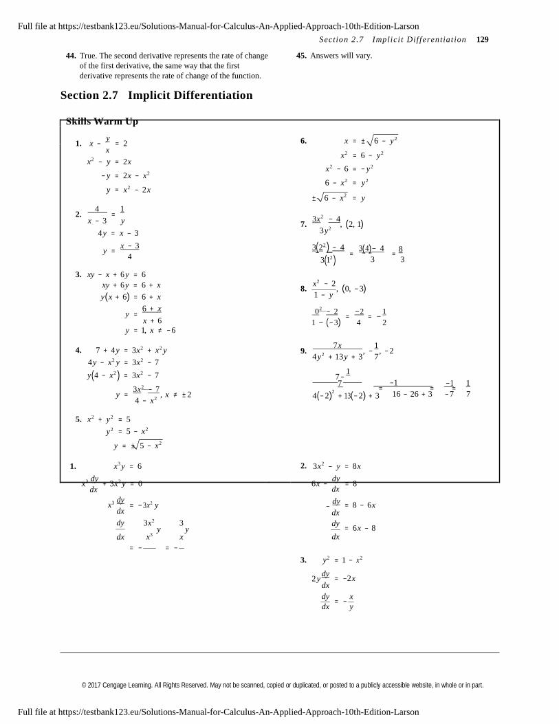
© 2017 Cengage Learning. All Rights Reserved. May not be scanned, copied or duplicated, or posted to a publicly accessible website, in whole or in part.
2
Section 2.7 Implici t Dif fe rentiat i on 129
44. True. The second derivative represents the rate of change
of the first derivative, the same way that the first
derivative represents the rate of change of the function.
Section 2.7 Implicit Differentiation
45. Answers will vary.
Skills Warm Up
1. x − y
= 2
6. x = ±
6 − y 2
x
x2 − y = 2 x x2 = 6 − y 2
− y = 2 x − x2 x2 − 6 = − y 2
y = x2 − 2x 6 − x2 = y 2
± 6 − x2 = y
2. 4
= 1
x − 3 y
4 y = x − 3
3x 2 − 4
7. 3 y2
, (2, 1)
y = x − 3
4
3. xy − x + 6 y = 6
3(22 ) − 4 3(4)− 4 8 = =
3(12 ) 3 3
x2 − 2xy + 6 y = 6 + x
y(x + 6) = 6 + x 8.
1 − y , (0, − 3)
y = 6 + x
02 − 2 −2 1
x + 6
y = 1, x ≠ − 6
= = − 1 − (− 3) 4 2
4. 7 + 4 y = 3x2 + x2 y
9. 7 x
, −
1 , − 2
4 y 2 + 13 y + 3
7 4 y − x2 y = 3x2 − 7
y(4 − x2 ) = 3x2 − 7
7 −
1
7 −1
−1 1
3x 2 − 7 = = =y = , x ≠ ± 2
4 − x2
4(− 2) + 13(− 2) + 3 16 − 26 + 3 − 7 7
5. x2 + y 2
y 2
= 5
= 5 − x2
y = ± 5 − x2
1. x3 y = 6 2. 3x2 − y = 8x
x3 dy + 3x2 y = 0
dx 6x −
dy = 8
dx
x3 dy
dx
dy
= −3x2 y
3x2 3
− dy
dx
dy
= 8 − 6 x
y y dx x3 x
= 6 x − 8 dx
= − = −
3. y 2
2 y dy
dx
= 1 − x2
= −2x
dy x = −
dx y
Full file at https://testbank123.eu/Solutions-Manual-for-Calculus-An-Applied-Approach-10th-Edition-Larson
Full file at https://testbank123.eu/Solutions-Manual-for-Calculus-An-Applied-Approach-10th-Edition-Larson
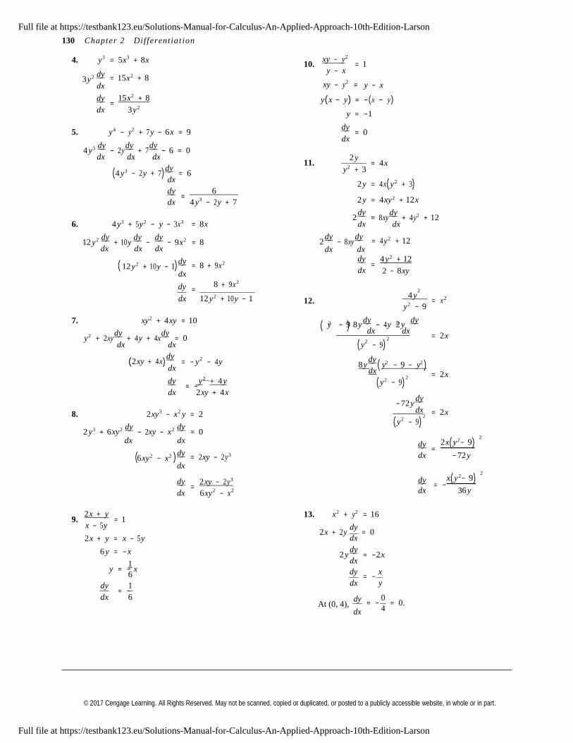
© 2017 Cengage Learning. All Rights Reserved. May not be scanned, copied or duplicated, or posted to a publicly accessible website, in whole or in part.
( )
2 2
2
( )
x
2
130 Chapte r 2 Dif ferentiat i on
4. y3 = 5x3 + 8x
10. xy − y 2
= 1
3 y 2 dy
dx
= 15x2 + 8 y − x
xy − y 2 =
y − x
dy =
dx
15 x2 + 8
3 y 2
y(x − y) = −(x − y)
y = −1
5. y4 − y 2 + 7 y − 6x = 9
4 y3 dy − 2 y
dy + 7
dy − 6 = 0
dy = 0
dx
dx dx dx
(4 y3 − 2 y + 7)dy = 6
11. 2 y
y 2 + 3 = 4x
dx
dy =
6 2 y = 4x( y 2 + 3)
2dx 4 y3 − 2 y + 7 2 y = 4xy + 12x
2 dy = 8xy
dy + 4 y 2 + 12
6. 4 y3 + 5 y2 − y − 3x3 = 8x dx dx
12 y 2 dy + 10 y
dy −
dy − 9x2 = 8
dx dx dx
2 dy
− 8xy dy
dx dx
= 4 y2 + 12
2
12 y 2 + 10 y − 1 dy
dx
dy
= 8 + 9x2
8 + 9x2
=
dy =
dx
4 y + 12
2 − 8xy
2
dx 12 y2 + 10 y − 1 12. 4 y
= x2
y 2 − 9
7. xy 2 + 4xy = 10 ( 2 )
dy 2 dy y − 9 8 y − 4 y 2 y
y2 + 2xy dy
+ 4 y + 4 x dy
= 0 dx dx
dx dx
( y − 9) = 2x
(2xy + 4x) dy
= − y2 − 4 y dy
(
2 2 )dx
dy y 2 + 4 y = −
8 y y − 9 − y dx
( y 2 − 9)
= 2x
dx 2 xy + 4x
− 72 y dy
dx 8. 2 xy3 − x2 y = 2
( y2 − 9) = 2x
2 y3 + 6xy2 dy − 2 xy − x2 dy
= 0
2 2
dx dx
6 xy2 − x2 dy
dx
= 2 xy − 2 y3
dy 2 x( y − 9) =
dx − 72 y
2 2
dy =
dx
2 xy − 2 y3
6xy 2 − x2
dy x( y − 9) = −
dx 36 y
9. 2 x + y
= 1 x − 5 y
13. x2 + y 2
dy
= 16
2x + y = x − 5 y 2 x + 2 y = 0
dx
6 y = − x 2 y dy
dx
= −2x1
y = − 6
dy 1 = −
dy x = −
dx y
dx 6 At (0, 4),
dy
dx
0 = − = 0.
4
Full file at https://testbank123.eu/Solutions-Manual-for-Calculus-An-Applied-Approach-10th-Edition-Larson
Full file at https://testbank123.eu/Solutions-Manual-for-Calculus-An-Applied-Approach-10th-Edition-Larson
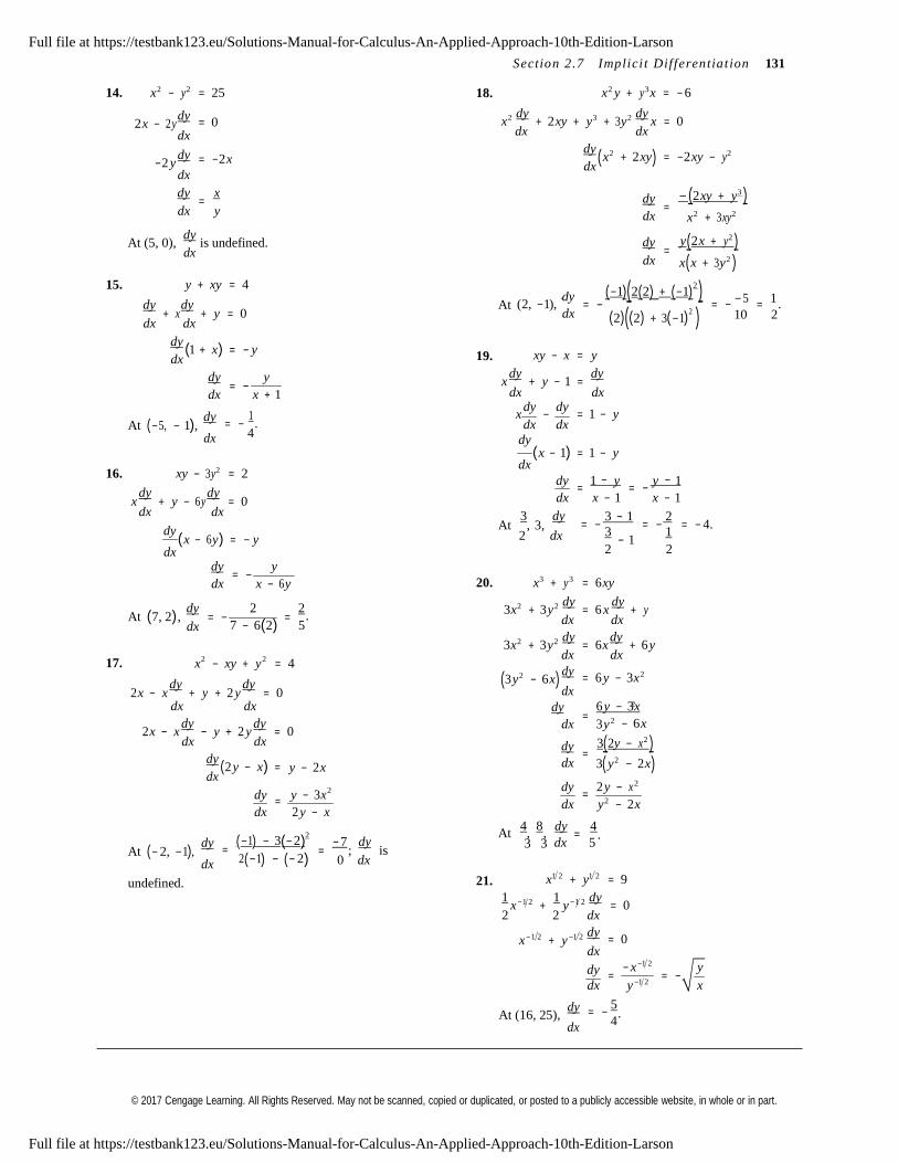
© 2017 Cengage Learning. All Rights Reserved. May not be scanned, copied or duplicated, or posted to a publicly accessible website, in whole or in part.
( )
−5 1
( )
=
3 3
.
= −
Section 2.7 Implici t Dif fe rentiat i on 131
14. x2 − y 2
2 x − 2 y dy
dx
−2 y dy
dx
= 25
= 0
= −2x
18. x2 y + y3 x = − 6
x2 dy + 2xy + y3 + 3 y2 dy
x = 0 dx dx
dy x2 + 2xy = −2 xy − y 2
dx
dy =
x dy − (2 xy + y3 )dx y
At (5, 0), dy
is undefined. dx
= dx
dy =
dx
x2 + 3xy 2
y(2 x + y 2 ) x(x + 3 y2 )
15. y + xy = 4 dy (−1)(2(2) + (−1)
2 ) dy
+ x dy
+ y = 0 dx dx
dy (1 + x) = − y
At (2, −1), dx (2)((2) + 3(−1)
2 ) = − = .
10 2
dx
dy = −
y
19. xy − x = y
x dy
+ y − 1 = dy
dx x + 1 dx dx dy dy
At (−5, − 1), dy
dx = −
1 .
4
x − dx dx
dy
= 1 − y
(x − 1) = 1 − y dx
16. xy − 3 y 2 = 2 dy 1
y y 1
= −
= − −
x dy
+ y − 6 y dy
= 0 dx x − 1 x − 1dx dx 3 dy 3 − 1 2
dy
(x − 6 y) = − y dx
At 2
, 3, dx
= − = − 3
− 1 1
2 2
= − 4.
dy = −
y
dx x − 6 y 20. x3 + y3
2 2 dy = 6 xy
dy dy
= − 2
= 2
3x + 3 y
dx = 6 x
dx + y
At (7, 2), dx
. 7 − 6(2) 5
3x2 + 3 y 2 dy
= 6 x dy
+ 6 y
17. x2 − xy + y 2 = 4 dx dx
2 x − x
dy + y
+ 2 y
dy = 0
3 y 2 − 6x dy
dx = 6 y − 3x2
dx
dx 2 dy 6 y − 3x
2
2 x − x dy
− y + 2 y dy
= 0 dx 3 y − 6x
dx dx
dy (2 y − x) =
dx
y − 2 x
dy 3(2y − x 2 ) =
dx 3( y 2 − 2x) dy 2 y − x2
dy y − 3x2
= = dx y 2 − 2 x
dx 2 y − x
4 8 dy 4.
At (− 2, −1), dy
dx
(−1) − 3( − 2) 2
= 2(−1) − (− 2)
= − 7
; dy
is 0 dx
At , , = dx 5
undefined. 21. x1 2 + y1 2 = 9
1 x−1 2 +
1 y−1 2 dy
= 02 2 dx
x−1 2 + y−1 2 dy
dx
dy
= 0
− x−1 2 y = = −
At (16, 25), dy
dx
dx y−1 2 x
5 = −
4
Full file at https://testbank123.eu/Solutions-Manual-for-Calculus-An-Applied-Approach-10th-Edition-Larson
Full file at https://testbank123.eu/Solutions-Manual-for-Calculus-An-Applied-Approach-10th-Edition-Larson

© 2017 Cengage Learning. All Rights Reserved. May not be scanned, copied or duplicated, or posted to a publicly accessible website, in whole or in part.
. ( )
( )
132 Chapte r 2 Dif ferentiat i on
22. x2 3 + y 2 3 = 5 25. y 2 (x2 + y2 ) = 2 x2
2 x−1 3 +
2 y −1 3 dy
= 0
y 2 2 x + 2 y dy
+ (x2 + y 2 ) 2 y dy
= 4 x3 3 dx
dx
dx
dy − x −1 3
y1 3 y
dy dy dy= = − = − 3 2 xy2 + 2 y3 + 2 x2 y + 2 y3 = 4 x
At (8, 1), dy
dx
dx y −1 3
1 = −
2
x1 3 x dx dx dx
dy 4 y3 + 2x2 y = 4 x − 2xy 2
dx
dy 2 x(2 − y 2 ) 23. xy = x − 2 y
x y = x − 2 y
x 1
y−1 2 dy + y
1 x−1 2 = 1 − 2
dy
= dx 2 y(2 y 2 + x2 ) dy x(2 − y 2 )
= dx y(2 y2 + x2 )
2 dx
2
dx
x dy dy + 2
y
= 1 −
At (1, 1),
dy
dx
= 1
. 3
2 y dx dx 2 x 2 2
2 2
1 − y
dy = 2 x ⋅
2 x y
26. (x
2 2
+ y ) dy
= 8x y
2 dydx x 2 x y
+ 2 2(x + y ) 2x + 2 y = 8x
dx + y(16 x)
dx2 y
4 x3 + 4x2 y dy
+ 4xy 2 + 4 y3 dy = 8x2 dy
+ 16xy2 xy − y
= x + 4 xy
dx dx dx
dy (4x2 y + 4 y3 − 8x2 ) = 16 xy − 4x3 − 4xy2
2( x − 2 y) − y =
x + 4(x − 2 y)
dx
dy =
4(4xy − x3 − xy 2 )2 x − 5 y
=
dx 4(x y + y
− 2x )
At (4, 1),
dy
dx
= 1
. 4
5x − 8 y
At (2, 2), dy
= 0.
2 3 2
dy x(4 y − x2 − y 2 ) =
dx x2 y + y3 − 2 x2
24. (x + y)3
= x3 + y3
3(x + y)2 1 +
dy = 3x2 + 3 y 2
dy
27.
3x2
dx
− 2 y + 5 = 0
dx dx 6x − 2
dy = 0
3(x + y)2
+ 3(x + y)2 dy
= 3x2 + 3 y 2 dy
dx dx
(x + y)2 dy
− y 2 dy
= x2 − (x + y)2
dx dx dy
(x + y)2
− y 2 = x2 − x2 + 2xy + y 2
dx
dx
dy = 3x
dx
At (1, 4), dy
= 3. dx
dy −(2 xy + y 2 ) = = − y(2 x + y)
28.
4x2 + 2 y − 1 = 0
At (−1, 1), dy
dx
= −1.
dx x2 + 2 xy x(x + 2 y)
8x + 2 dy
dx
dy
= 0
8x = −4x= −
dx 2
dy (−1) = −4(−1) = 4
dx
Full file at https://testbank123.eu/Solutions-Manual-for-Calculus-An-Applied-Approach-10th-Edition-Larson
Full file at https://testbank123.eu/Solutions-Manual-for-Calculus-An-Applied-Approach-10th-Edition-Larson
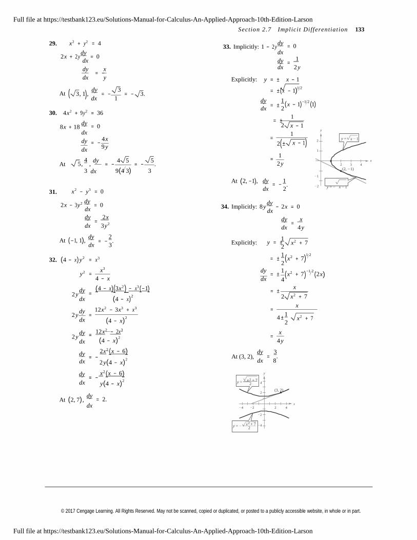
© 2017 Cengage Learning. All Rights Reserved. May not be scanned, copied or duplicated, or posted to a publicly accessible website, in whole or in part.
) = ±
4
.
.
= ± ( )
4
4
= −
( )
Section 2.7 Im plici t D i ffe r e ntiat i on 133
29. x2 + y 2 = 4
2 x + 2 y dy
= 0 dx
33. Implicitly: 1 − 2 y dy
dx
dy
= 0
= 1
dy x = −
dx 2 y
dx y Explicitly: y = ± x − 1
1 2
At ( 3, 1 , dy
= − 3
dx 1 = − 3.
= ±(x − 1)
dy 1 (x − 1)
−1 2 (1)
dx 230. 4 x2 + 9 y 2
8x + 18 dy
dx
dy
dx
= 36
= 0
4 x = −
9 y
= ± 2
= 2(±
1
1
x − 1 y
1
x − 1) 2
1
y = x − 1
At dy 5, ,
3
4 5 5 = − = − .
= 2 y 2
x
3 4
(2, − 1) dx 9(4 3) 3
At (2, −1), − 1
dy 1 = − − 2
31. x2 − y3 = 0 dx 2 y = − x − 1
2 x − 3 y2 dy = 0
dx
34. Implicitly: 8 y dy
− 2x = 0 dx
dy =
2 x dx 3 y 2
dy =
x dx 4 y
At (−1, 1), dy 2 dx 3
Explicitly:
1 y = ±
2
x2 + 7
32. (4 − x) y 2
= x3
1 x2 + 7
1 2
2
x3 dy 1
−1 2 y 2 =
4 − x = ± x2 + 7 (2 x)
dx
2 y dy
dx
dy
(4 − x)(3x2 ) − x3 (−1) =
(4 − x)2
12x2 − 3x3 + x3
= ± x
2 x2 + 7
= x
2 y = dx (4 − x)
2 1
4 ± 2 x2 + 7
2 y dy
dx
dy
12 x2 − 2 x3
= (4 − x)
2
2 x2 ( x − 6)
= x
4 y
dy 3= −
dx 2 y(4 − x)2
dy x2 ( x − 6)
= −
At (3, 2),
2
= . dx 8
y
dx y(4 − x)2
y = x + 7 2
2
(3, 2)
At (2, 7), dy
dx = 2.
x − 4 − 2 2 4
− 2
y = − x 2 + 7 − 4 2
Full file at https://testbank123.eu/Solutions-Manual-for-Calculus-An-Applied-Approach-10th-Edition-Larson
Full file at https://testbank123.eu/Solutions-Manual-for-Calculus-An-Applied-Approach-10th-Edition-Larson
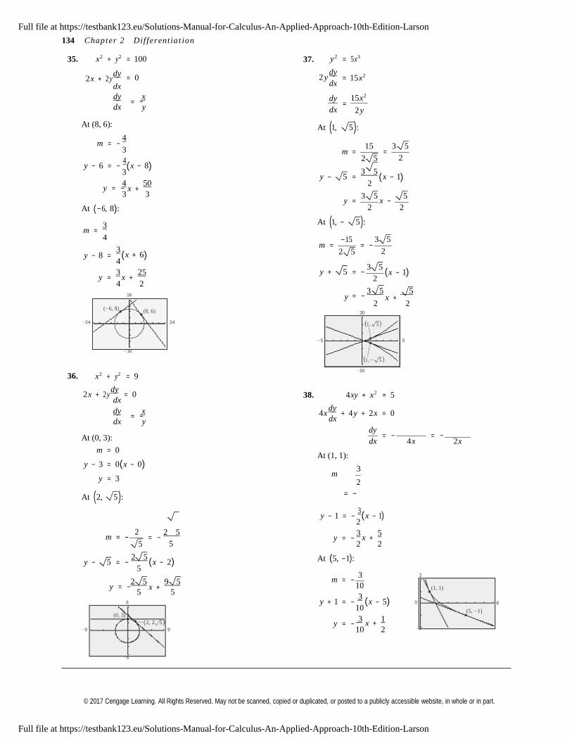
© 2017 Cengage Learning. All Rights Reserved. May not be scanned, copied or duplicated, or posted to a publicly accessible website, in whole or in part.
x +
x +
x +
x +
x +
= −
4
134 Chapte r 2 Dif ferentiat i on
35. x2 + y 2
2 x + 2 y dy
dx
= 100
= 0
37. y2
2 y dy
dx
= 5x3
= 15x2
dy x = −
dx y dy
= dx
15x2
2 y
At (8, 6):
m 4
At (1, 5 ):
3 m = 15
= 3 5
y − 6 = − 4 (x − 8)
2 5 2
3
4 50 y = −
3 3
y − 5 = 3 5
(x − 1) 2
3 5 5
At (−6, 8): y = x −
2 2
m = 3
At (1, − 5 ):
m = −15
= − 3 5
y − 8 = 3 (x + 6)
4
2 5 2
3 5
y = 3
x + 25
4 2
y + 5 = − (x − 1) 2
16 y 3 5 5
= −
(− 6, 8) 2 2
(8, 6) 30
− 24 24 (1, 5 )
− 5 5
− 16
(1, − 5 )
36.
x2 + y 2 = 9
2 x + 2 y dy
= 0 dx
dy x = −
dx y
38.
− 30
4 xy + x2 = 5
4 x dy
+ 4 y + 2x = 0 dx
dyAt (0, 3):
m = 0
y − 3 = 0(x − 0)
y = 3
At (1, 1):
m 3
2
= − = − dx 4x 2 x
At (2, 5): = −
y − 1 = − 3 (x − 1)
2
m = − 2 5
= − 2 5
5
3 5 y = −
2 2
y − 5 = − 2 5
(x − 2) 5
At (5, −1):
3 2
2 5 9 5 y = −
5 5 6
(0, 3)
m = − 10
y + 1 = − 3
(x − 5) 10
(1, 1)
0
8
(5, − 1)
( 2, 2 5 ) − 9 9
3 1 y = −
10 2 − 2
− 6
Full file at https://testbank123.eu/Solutions-Manual-for-Calculus-An-Applied-Approach-10th-Edition-Larson
Full file at https://testbank123.eu/Solutions-Manual-for-Calculus-An-Applied-Approach-10th-Edition-Larson
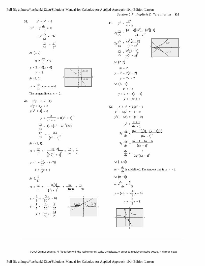
© 2017 Cengage Learning. All Rights Reserved. May not be scanned, copied or duplicated, or posted to a publicly accessible website, in whole or in part.
(− 1, 0)
(0, − 1)
( )
5
= −
x +
0
( )
(
2
2
Section 2.7 Implici t Diffe r entiat i o n 135
39. x3 + y3 = 8
3x2 + 3 y 2 dy = 0
41.
y 2 = x3
4 − x
dx
3 y 2 dy
= −3x2
2 y dy
dx
(4 − x)(3x 2 ) − ( x3 )(−1) =
(4 − x)2
dx
dy x2 = −
dx y 2
2 y dy
dx
3
2 x 2 (6 − x) =
(4 − x)2
(2, 2)
4
At (0, 2):
m = dy
= 0
dy x 2 (6 − x) =
dx y 4 − x 2
− 3
(2, − 2)
dx
y − 2 = 0(x − 0)
y = 2
At (2, 0): − 8
5
(0, 2)
8
(2, 0)
At (2, 2):
m = 2
y − 2 = 2(x − 2)
y = 2 x − 2
m = dy
is undefined. dx − 5
At (2, − 2):
m = −2
40.
The tangent line is x = 2.
x2 y − 8 = − 4 y
y + 2 = −2(x − 2)
y = −2 x + 2
x2 y + 4 y = 8
y(x2 + 4) = 8
42.
x + y3
y3 − 6xy3
= 6xy3 − 1
= −1 − x
y = 8
= 8 x2 + 4 −1
y3 (1 − 6x) = − (1 + x)x2 + 4
( ) dy 2
− 2
y3 =
x + 1
= 8(−1) x dx
+ 4) (2x) 6x − 1
dy 16 x 3 y 2 dy (6 x − 1)(1) − ( x + 1)(6) =
= − dx (x2
+ 4) dx (6 x − 1)
2
At (− 2, 1): 3 y 2 dy
dx =
6 x − 1 − 6 x − 6
(6x − 1)2
m = dy 16(− 2) 32 1
= − = =
dy 7dx ((− 2)
2
+ 4) 64 2 = −
dx 3 y 2 (6 x − 1)2
y − 1 = 1 (x − (− 2))
2 At (−1, 0):
y = 1
x + 2 2
m = dy
is undefined. The tangent line is x = −1. dx
At 6,
1 : At (0, −1):
5
dy 7
m = dy 16(6) 96 3
= − = − = − m = = −
dx 3dx 6
2 + 4
2
1600 50
y − (−1) = −
7 (x − 0)
y − 1
= − 3
(x − 6) 5 50
y − 1
= − 3
x + 9
5 50 25
5
(− 2, 1) (6,
1 ) − 8 8
3
y 7
x − 1 3
2
3 14 y = −
50 25 − 5
− 3 3
− 2
Full file at https://testbank123.eu/Solutions-Manual-for-Calculus-An-Applied-Approach-10th-Edition-Larson
Full file at https://testbank123.eu/Solutions-Manual-for-Calculus-An-Applied-Approach-10th-Edition-Larson
© 2017 Cengage Learning. All Rights Reserved. May not be scanned, copied or duplicated, or posted to a publicly accessible website, in whole or in part.
( )
136 Chapte r 2 Dif ferentiat i o n
43. p = 2
, x ≥ 0 0.00001x3 + 0.1x
46. p =
500 − x , 0 < x ≤ 500
2x
0.00001x3 + 0.1x = 2
2 xp2 = 500 − x
p 2 x(2 p) + p2
2
dx = −
dx
0.00003x2 dx + 0.1
dx = − 2 dp dp
dp dp p2 dx
(2 p2 + 1) = −4xp
(0.00003x2 + 0.1) dx = −
2 dp
dp p2 dx
= − 4xp 2
dx = −
2 dp 2 p + 1
44.
dp p2 (0.00003x2 + 0.1)
p = 4
, x ≥ 0
47. (a)
100x0.75 y0.25 = 135,540
100x0.75 0.25 y −0.75 dy + y0.25 (75x−0.25 ) = 0
0.000001x2 + 0.05x + 1
dx
0.000001x2 + 0.05x + 1 = 4 p
25x0.75
y0.75
⋅ dy
= − dx
dy
75 y0.25
x0.25
3 y
0.000002 x dx
+ 0.05 dx = −
4 = − dx x
dp dp p2
(0.000002x + 0.05) dx
dp
dx
= − 4 p2
= − 4
(b)
When x = 1500 and y = 1000, dy
dx 100,000
= −2.
dp p2 (0.000002x + 0.05)
45. p = 200 − x
, 0 < x ≤ 200 2 x
0 2,000
0
2 xp2 = 200 − x
If more labor is used, then less capital is available.
2 x(2 p) + p2 2 dx
= − dx If more capital is used, then less labor is available.
dp
dp
2 p2 + 1 dx
dp
dx
= −4xp
= − 4xp
48. (a) As price increases, the demand decreases.
(b) For x > 0, the rate of change of demand, x, with
respect to the price, p, is always decreasing; that is,
dxdp 2 p2 + 1 for x > 0, is never increasing.
dp
49. (a) y 2 − 35,892.5 = − 27.0021t 3 + 888.789t 2 − 9753.25t
y 2 = − 27.0021t 3 + 888.789t 2 − 9753.25t + 35,892.5
y = ± − 27.0021t 3 + 888.789t 2 − 9753.25t + 35,892.5
40
8 12 0
The numbers of cases of Chickenpox decreases from 2008 to 2012.
(b) It appears that the number of reported cases was decreasing at the greatest rate during 2008, t = 8.
Full file at https://testbank123.eu/Solutions-Manual-for-Calculus-An-Applied-Approach-10th-Edition-Larson
Full file at https://testbank123.eu/Solutions-Manual-for-Calculus-An-Applied-Approach-10th-Edition-Larson
© 2017 Cengage Learning. All Rights Reserved. May not be scanned, copied or duplicated, or posted to a publicly accessible website, in whole or in part.
Section 2.8 Related Rates 137
(c) y2 − 35,892.5 = − 27.0021t 3 + 888.789t 2 − 9753.25t
2 y dy
dt
= − 81.0063t 2 + 1777.578t − 9753.25t
y′ = dy
= dt
− 81.0063t 2 + 1777.578t − 9753.25
2 y
t 8 9 10 11 12
y 30.40 20.51 15.39 14.51 13.40
y′ −11.79 − 7.71 − 2.54 − 0.06 − 3.26
The table of values for y′ agrees with the answer in part (b) when the greatest value of y′ is −11.79 thousand cases
per year.
Section 2.8 Related Rates
Skills Warm Up
1. A = π r 2 9. x2 + 2 y + xy = 12
2. V
= 4π r3 d x2 + 2 y + xy =
d (12)
3
3. SA = 6s2
dx dx
2 x + 2 dy
+ y + x dy
= 0 dx dx
4. V
5. V
= s3
= 1π r 2h
dy dy 2 + x
dx dx
= − y − 2x
6. A =
3
1 bh
dy (2 + x) = − y − 2x
dx2
7. x2 + y 2 = 9
dy =
− y − 2 x
dx 2 + x
d x2 + y2 =
d [9]
10. x + xy 2 − y 2 = xy
dx dx
2x + 2 y dy
= 0
d x + xy2 − y2 =
d [xy]
dx dx
dx 1 + y 2 + 2 xy dy
− 2 y dy = y + x
dy
2 y dy
= −2x dx dx dx
dx
dy =
−2 x 2xy
dy − 2 y
dy − x
dy
dx dx dx = y − y 2 − 1
dx 2 y
= − x
dy (2 xy − 2 y − x) =
dx y − y 2 − 1
2
y
8. 3xy − x2 = 6
dy y − y − 1 =
dx 2 xy − 2 y − x
d 3xy − x2 =
d [6]
dx dx
3 y + 3x dy
− 2 x = 0 dx
3x dy
dx
= 2x − 3 y
dy =
2 x − 3 y
dx 3x
Full file at https://testbank123.eu/Solutions-Manual-for-Calculus-An-Applied-Approach-10th-Edition-Larson
Full file at https://testbank123.eu/Solutions-Manual-for-Calculus-An-Applied-Approach-10th-Edition-Larson
© 2017 Cengage Learning. All Rights Reserved. May not be scanned, copied or duplicated, or posted to a publicly accessible website, in whole or in part.
2 4
= −
= −
= −
= −
)
138 Chapte r 2 Dif ferentiat i on
1. y = x , dy =
1 x−1 2
dx 1 dx dx = , = 2 x
dy
dt 2 dt 2 x dt dt dt
(a) When x = 4 and dx
dt
dy = 3,
dt
= 1
(3) = 3
. 4
(b) When x = 25 and dy
dt
= 2, dx
dt
= 2 25(2) = 20.
2. y = 3x2 − 5x, dy
= 6x dx
− 5 dx
, dy
dy
= (6x − 5) dx
, dt = dx
dt dt dt dt dt 6x − 5 dt
(a) When x = 3 and dx
dt
= 2, dy
dt
= (6(3) − 5(2)) = 26.
(b) When x = 2 and dy
= 4, 4
= 4
=
dx.
3. xy = 4, x dy
+ y dx
dt
= 0, dy
6(2) − 5 7
= −
y dx ,
dx
dt
x dy
= −
dt dt dt x dt dt
y
dt
(a) When x = 8, y =
1 , and
dx
= 10,
= − (10) = − .2 dt
dy 1 2 5
dt 8 8
(b) When x = 1, y = 4, and dy
= − 6, dx 1
(− 6) = 3
.dt dt 4 2
4. x2 + y 2
= 25, 2 x dx
+ 2 y dy
dt dt = 0,
dy x dx ,
dt y dt
dx y dy = −
dt x dt
(a) When x = 3, y = 4, and dx
dt
= 8, dy
dt
3 (8) = − 6.
4
(b) When x = 4, y = 3, and dy
= −2, dx 3
(−2) = 3
.
5. A = π r 2 , dr
= 3,
dt
dA
= 2π r dr
dt
= 6π r
4 2
8. V
= 4π r 3 ,
dV
= 4π r 2 dr
dt dt dt 3 dt dt
(a) When r = 6, dA
= 2π (6)(3) = 36π in.2 min.
If dr
is constant, dV
is not constant since it isdt dt dt
(b) When r = 24, dA
= 2π (24)(3) = 144π in.2 min. dt
proportional to the square of r.
9. V = 4π r 3 ,
dV = 10, dV = 4π r 2 dr
,
6. V
= 4π r 3 ,
dr = 3,
dV = 4π r 2 dr
= 12π r 2
3 dt dt dt
3 dt dt dt dr =
1 dV
dt 4π r 2 dt
(a) When r = 9, dV dt
= 12π (9)2 = 972π in.3 min.
(a) When r = 1, dr
=
1 5
2 (10) =
ft min.
(b) When r = 16, dV
= 12π (16)2
= 3072π in.3 min. dt 4π (1) 2π
dt
7. A = π r 2 ,
dA = 2π r
dr
dt dt
If dr
is constant, then dA
is not constant; dA
is
(b) When r = 2, dr
dt
1 5 =
4π (2 2 (10) =
8π ft min.
dt dt dt
proportional to r.
Full file at https://testbank123.eu/Solutions-Manual-for-Calculus-An-Applied-Approach-10th-Edition-Larson
Full file at https://testbank123.eu/Solutions-Manual-for-Calculus-An-Applied-Approach-10th-Edition-Larson
© 2017 Cengage Learning. All Rights Reserved. May not be scanned, copied or duplicated, or posted to a publicly accessible website, in whole or in part.
13
Section 2.8 Related Rates 139
10. V = 1π r 2 h =
1π r 2 (3r ) = π r 3
14. R = 510x − 0.3x2 , dR = 510
dx − 0.6 x
dx ,
3 3 dt dt dt
dV = 3π r 2
dr
= 6π r 2
dR = (510 − 0.6x)
dx
dt dt dt dt
dx(a) When r = 6,
dV dt
= 6π (6)2 = 216π in.3 min. (a) When
dt
dR
= 9 units day and x = 400 units,
(b) When r = 24, dV dt
= 6π (24)2 = 3456π in.3 min.
= 510 − 0.6(400)(9) = $2430 per day. dt
11. (a)
dC
= 0.75 dx
= 0.75(150) (b) When
dx
dt = 9 units day and x = 600 units,
dt dt
= 112.5 dollars per week
dR = 510 − 0.6(600)(9) = $1350 per day.
dt
(b)
dR = 250
dx −
1 x
dx dx dV dx
dt dt 5 dt 15. V = x3 , = 6, = 3x2
= 250(150) − 1 (1000)(150)
dt dt dt
(c)
5
= 7500 dollars per week
P = R − C
(a) When x = 2,
(b) When x = 10,
dV = 3(2)
2 (6) = 72 cm3 sec.
dt
dV = 3(10)
2 (6) = 1800 cm3 sec.
dtdP dR dC
= − = 7500 − 112.5dt dt dt dx dA dx
16. A = 6 x2 , = 6, = 12 x= 7387.5 dollars per week dt dt dt
dA = 12 2 6
= 144 cm2 sec.
12. (a) dC
= 1.05 dx = 1.05(250) = 262.5 dollars week (a) When x = 2,
dt ( )( )
dt dt
dA = 12 10 6
= 720 cm2 sec.
(b) dR
= 500 − 2 x dx 2(5000)
= 500 − (250)
(b) When x = 10,
dt ( )( )
dt 25 dt 25
(c)
= 25,000 dollars week
P = R − C
17. Let x be the distance from the boat to the dock and y be
the length of the rope.
dP dR dC = −
= 25,000 − 262.5
122 + x2 = y 2
dydt dt dt
= 24,737.5 dollars week
dt
2 x dx
= − 4
= 2 y dy
13. R = 1200 x − x2 , dR
= 1200 dx
− 2 x dx
, dt dt
dt dt dt dx y dy =
dR = (1200 − 2 x)
dx dt x dt
dt dt When y = 13, x = 5 and
(a) When dx
dt
= 23 units day and x = 300 units, dx
= (− 4) = −10.4 ft sec. dt 5
dR = 1200 − 2(300)(23) = $13,800 per day.
dt As x → 0,
dx increases.
dt
(b) When dx
dt
= 23 units day and x = 450 units,
dR = 1200 − 2(450)(23) = $6900 per day.
dt
Full file at https://testbank123.eu/Solutions-Manual-for-Calculus-An-Applied-Approach-10th-Edition-Larson
Full file at https://testbank123.eu/Solutions-Manual-for-Calculus-An-Applied-Approach-10th-Edition-Larson
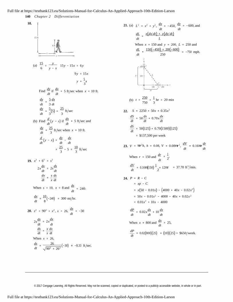
© 2017 Cengage Learning. All Rights Reserved. May not be scanned, copied or duplicated, or posted to a publicly accessible website, in whole or in part.
5
2
10
y
dt
140 Chapte r 2 Dif ferentiat i on
18.
21. (a)
L 2 = x2 + y 2 , dx
dt
= − 450, dy
dt
= − 600, and
dL x(dx dt ) + y(dy dt ) =
15 ft 6 ft
dt L
When x = 150 and y = 200, L = 250 and
dL x
dt
150(− 450) + 200(− 600) =
250 y
= −750 mph.
(a) 15
= y
15 y − 15x = 6 y6 y − x
9 y = 15x
y = 5
x 3
200
y 100
L
x 100 200
Find dy
if dx = 5 ft sec when x = 10 ft. x
dt dt
dy 5 dx (b)
t = 250
1
= hr = 20 min=
dt 3 dt 750 3
dy = (5) = 25
ft sec
22.
S = 2250 + 50 x + 0.35x2
dt 3 3
dS dx dx
(b) Find d
( y − x) if dx = 5 ft sec and
= 50 dt dt
+ 0.70 x dt
dt dt dS
dy =
25 ft sec when x = 10 ft.
dt 3
= 50(125) + 0.70(1500)(125) dt
= $137,500 per week d
( y − x) = dy −
dx
dt dt dt
23. V
= π r 2h, h = 0.08, V
= 0.08π r 2 , dV
= 0.16π r dr
19.
x2 + 62
= s2
= 25
− 5 = 10
ft sec 3 3
When r = 150 and dr
dt
= 1 ,
2
dt dt
2 x dx
= 2s ds dV
= 0.16π (150) 1
= 12π
= 37.70 ft3 min.dt dt
dx s ds =
dt x dt
When s = 10, x = 8 and ds
= 240:
24.
P = R − C
= xp − C
dt = x(50 − 0.01x) − (4000 + 40 x − 0.02 x2 ) 2 2dx
= (−240) = 300 mi hr. = 50 x − 0.01x − 4000 − 40 x + 0.02 x
dt 8 = 0.01x2 + 10 x − 4000
20.
s 2 = 902 + x2 , x = 26, dx
= −30
dP
= 0.02 x dx
+ 10 dx
2s ds
dt
= 2 x dx
dt dt dt
When x = 800 and dx
= 25,
dt dt
ds x dx =
dt s dt
When x = 26,
dt
dP = 0.02(800)(25) + (10)(25) = $650 week.
dt
ds 26 = (−30) ≈ −8.33 ft sec.
dt 902 + 262
Full file at https://testbank123.eu/Solutions-Manual-for-Calculus-An-Applied-Approach-10th-Edition-Larson
Full file at https://testbank123.eu/Solutions-Manual-for-Calculus-An-Applied-Approach-10th-Edition-Larson
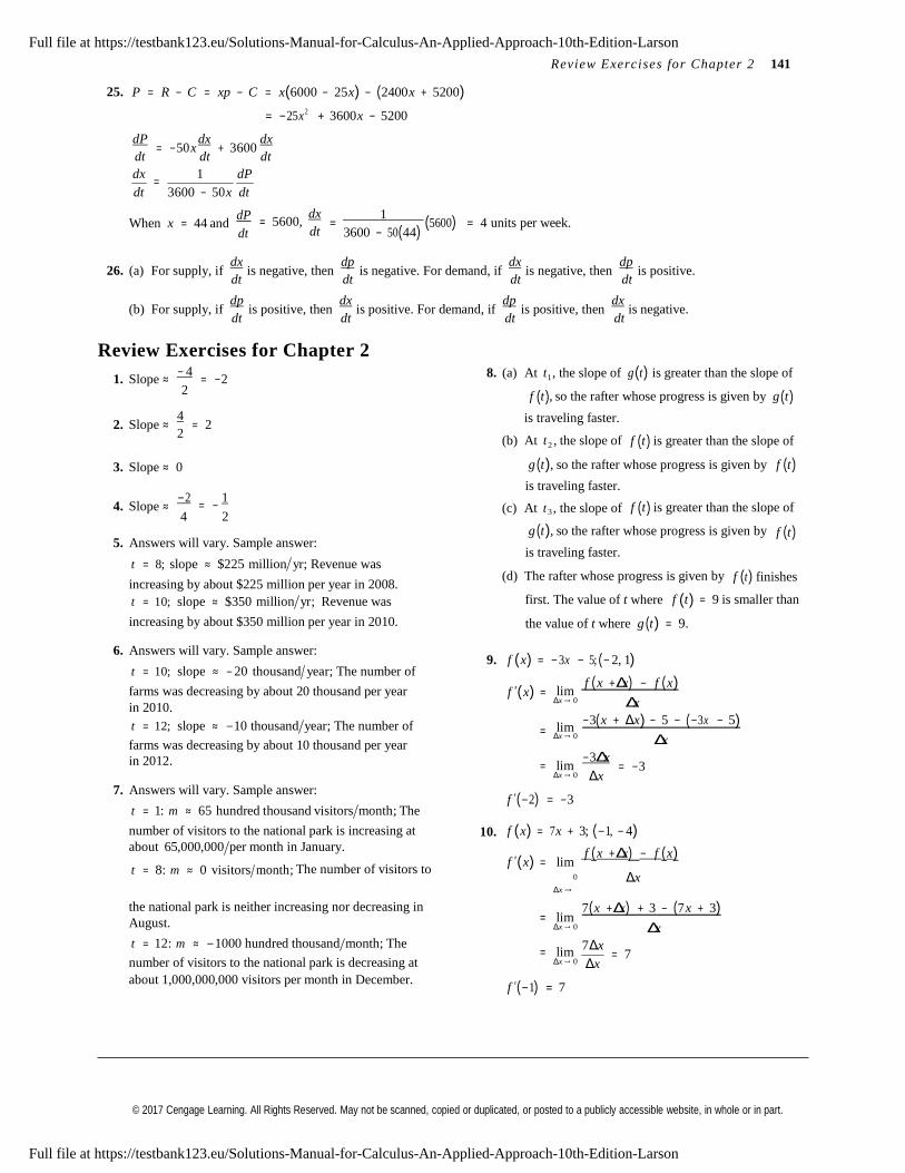
© 2017 Cengage Learning. All Rights Reserved. May not be scanned, copied or duplicated, or posted to a publicly accessible website, in whole or in part.
Review Exercises for Chapter 2 141
25. P = R − C = xp − C = x(6000 − 25x) − (2400 x + 5200)
= −25x2 + 3600x − 5200
dP = −50 x
dx + 3600
dx dt dt dt
dx 1 dP =
dt 3600 − 50 x dt
When x = 44 and dP dt
dx = 5600,
dt
1 = (5600) = 4 units per week.
3600 − 50(44)
26. (a) For supply, if dx
is negative, then dp
is negative. For demand, if dx
is negative, then dp
is positive.dt dt dt dt
(b) For supply, if dp
is positive, then dx
is positive. For demand, if dp
is positive, then dx
is negative.dt dt dt dt
Review Exercises for Chapter 2
1. Slope ≈ − 4
2
= −2 8. (a) At t1 , the slope of g(t) is greater than the slope of
f (t ), so the rafter whose progress is given by g(t)
2. Slope ≈ 4
= 2 2
is traveling faster.
(b) At t 2 , the slope of
f (t) is greater than the slope of
3. Slope ≈ 0 g (t ), so the rafter whose progress is given by
is traveling faster.
f (t)
4. Slope ≈ −2 1 = −
(c) At t , the slope of f (t) is greater than the slope of4 2
5. Answers will vary. Sample answer:
t = 8; slope ≈ $225 million yr; Revenue was
3
g (t ), so the rafter whose progress is given by
is traveling faster.
f (t)
increasing by about $225 million per year in 2008. (d) The rafter whose progress is given by f (t) finishes
t = 10; slope ≈ $350 million yr; Revenue was first. The value of t where f (t) = 9 is smaller than
increasing by about $350 million per year in 2010.
6. Answers will vary. Sample answer:
t = 10; slope ≈ − 20 thousand year; The number of
the value of t where g (t ) = 9.
9. f (x) = −3x − 5; (− 2, 1)
farms was decreasing by about 20 thousand per year
in 2010.
t = 12; slope ≈ −10 thousand year; The number of
farms was decreasing by about 10 thousand per year
f ′(x) =
=
lim Δx → 0
lim Δx → 0
f ( x +Δx) − f ( x) Δx
−3( x + Δx) − 5 − (−3x − 5) Δx
in 2012.
7. Answers will vary. Sample answer:
= lim Δx → 0
−3Δx
Δx = −3
t = 1: m ≈ 65 hundred thousand visitors month; The
number of visitors to the national park is increasing at
about 65,000,000 per month in January.
10.
f ′(−2) = −3
f (x) = 7 x + 3; (−1, − 4)
f ( x +Δx) − f ( x)t = 8: m ≈ 0 visitors month; The number of visitors to
f ′(x) = lim 0 Δx
the national park is neither increasing nor decreasing in
August.
t = 12: m ≈ −1000 hundred thousand month; The
number of visitors to the national park is decreasing at
Δx →
= lim Δx → 0
= lim Δx → 0
7( x +Δx) + 3 − (7 x + 3) Δx
7Δx = 7
Δx
about 1,000,000,000 visitors per month in December. f ′(−1) = 7
Full file at https://testbank123.eu/Solutions-Manual-for-Calculus-An-Applied-Approach-10th-Edition-Larson
Full file at https://testbank123.eu/Solutions-Manual-for-Calculus-An-Applied-Approach-10th-Edition-Larson
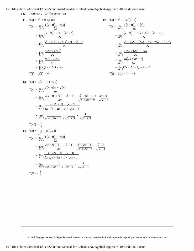
© 2017 Cengage Learning. All Rights Reserved. May not be scanned, copied or duplicated, or posted to a publicly accessible website, in whole or in part.
142 Chapte r 2 Dif ferentiat i on
11. f (x) = x2 + 9; (3, 18) 12. f (x) = x2 − 7 x; (1, − 6)
f ′(x) = f ( x +Δx) − f ( x) lim
f ′(x) = f ( x +Δx) − f ( x) lim
Δx → 0
= lim
Δx → 0
= lim
Δx → 0
= lim
Δx → 0
Δx
( x +Δx)2
+ 9 − ( x2 + 9) Δx
x2 + 2 xΔx + (Δx)2
+ 9 − x2 − 9
Δx
2 xΔx + (Δx)2
Δx
Δx →0
= lim Δx →0
= lim Δx →0
= lim Δx →0
Δx
( x +Δx)2
− 7( x + Δx) − ( x2 − 7 x) Δx
x2 + 2 xΔx + (Δx)2
− 7 x − 7Δx − x2 + 7 x
Δx
2 xΔx + (Δx)2
− 7Δx
Δx
= lim Δx(2 x + Δx) Δx(2 x + Δx − 7) = lim
Δx → 0 Δx Δx →0 Δx
= lim (2x + Δx) = 2x Δx → 0
= lim (2x + Δx − 7) = 2x − 7 Δx →0
f ′(3) = 2(3) = 6 f ′(1) = 2(1) − 7 = −5
13. f (x) =
f ′(x) =
x + 9; (−5, 2)
f ( x +Δx) − f ( x) limΔx → 0 Δx
= lim x +Δx + 9 − x + 9
⋅ x + Δx + 9 + x + 9
Δx → 0 Δx x + Δx + 9 + x + 9
= lim ( x +Δx + 9) − ( x + 9)
Δx → 0 Δx x + Δx + 9 + x + 9
= lim 1
= 1
Δx → 0 x + Δx + 9 + x + 9 2 x + 9
f ′(− 5) = 1 4
14. f (x) =
f ′(x) =
x − 1; (10, 3)
f ( x +Δx) − f ( x) limΔx → 0 Δx
= lim x +Δx − 1 − x − 1
⋅ x + Δx − 1 + x − 1
Δx → 0 Δx x + Δx − 1 + x − 1
= lim ( x +Δx − 1) − ( x − 1)
Δx → 0 Δx x + Δx − 1 + x − 1
= lim 1
= 1
Δx → 0
f ′(10) = 1 6
x + Δx − 1 + x − 1 2 x − 1
Full file at https://testbank123.eu/Solutions-Manual-for-Calculus-An-Applied-Approach-10th-Edition-Larson
Full file at https://testbank123.eu/Solutions-Manual-for-Calculus-An-Applied-Approach-10th-Edition-Larson
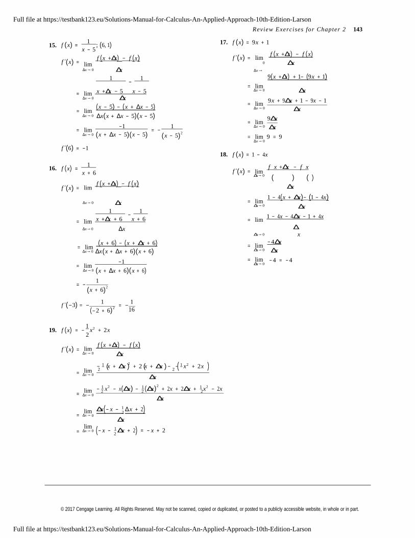
© 2017 Cengage Learning. All Rights Reserved. May not be scanned, copied or duplicated, or posted to a publicly accessible website, in whole or in part.
2
2
( ) ( ) ( )
2 2 2
Review Exer cis e s for Chapter 2 143
15. f (x) = 1
; (6, 1) x − 5
17. f (x) = 9x + 1
f ′(x) = f ( x +Δx) − f ( x)
lim
f ′(x) =
lim 0
f ( x +Δx) − f ( x) Δ x
Δx → 0 Δx
1 −
1
Δx →
= lim
9( x +Δx) + 1− (9 x + 1)
= lim x +Δx − 5 x − 5 Δx → 0 Δ xΔx → 0
= lim
Δx
( x − 5) − ( x + Δx − 5)
= lim Δx → 0
9x + 9Δ x + 1 − 9 x − 1
Δ xΔx → 0 Δx(x + Δx − 5)(x − 5)
= lim −1
= − 1
= lim Δx → 0
9Δ x
Δ xΔx → 0 (x + Δx − 5)(x − 5) (x − 5)
2
f ′(6) = −1
= lim 9 = 9 Δx → 0
16.
f (x) = 1
18. f (x) = 1 − 4 x
f x +Δx − f x
f ′(x) =
x + 6
f ( x +Δx) − f ( x) lim
f ′(x) = lim Δx → 0 ( ) ( )
Δ x
1 − 4( x + Δ x)− (1 − 4 x)Δx → 0 Δx
1 −
1
= lim Δx → 0 Δ x
1 − 4 x − 4Δ x − 1 + 4 x= lim x +Δx + 6 x + 6 = lim
ΔΔx → 0 Δx Δx → 0 x
= lim ( x + 6) − ( x + Δx + 6)
Δx → 0 Δx(x + Δx + 6)(x + 6)
= lim −1
Δx → 0 (x + Δx + 6)(x + 6)
= lim Δx → 0
= lim Δx → 0
− 4Δ x
Δ x
− 4 = − 4
= − 1
(x + 6)2
1 1f ′(−3) = − = −
(− 2 + 6)2 16
19.
f (x) 1
x2 + 2x= − 2
f ′(x) =
=
=
=
=
lim Δx → 0
lim Δx → 0
lim Δx → 0
lim Δx → 0
lim Δx → 0
f ( x +Δx) − f ( x) Δ x
− 1 x + Δ x 2
+ 2 x + Δ x − − 1 x2 + 2x 2 2
Δ x
− 1 x2 − x(Δ x) − 1 (Δ x)2
+ 2 x + 2Δ x + 1 x2 − 2 x
Δ x
Δ x(− x − 1 Δ x + 2) Δ x
(− x − 1 Δ x + 2) = − x + 2
Full file at https://testbank123.eu/Solutions-Manual-for-Calculus-An-Applied-Approach-10th-Edition-Larson
Full file at https://testbank123.eu/Solutions-Manual-for-Calculus-An-Applied-Approach-10th-Edition-Larson
© 2017 Cengage Learning. All Rights Reserved. May not be scanned, copied or duplicated, or posted to a publicly accessible website, in whole or in part.
4
144 Chapte r 2 Dif ferentiat i on
20. f (x) = 3x2 − 1
x 4
f ′(x) =
lim Δx → 0
f ( x +Δx) − f ( x) Δ x
3(x + Δ x)2 −
1 (x + Δ x)
− 3x2 − 1
x = lim
Δx → 0
= lim Δx → 0
= lim Δx → 0
= lim
Δx → 0
= lim
4 4
Δ x
3x2 + 6 x(Δ x) + 3(Δ x)2
− 1
x − 1 Δ x − 3x2 +
1 x
4 4 4 Δ x
6x(Δ x) + 3(Δ x)2
− 1 Δ x
4 Δ x
Δ x 6x + 3(Δ x) −
1
Δ x
6x + 3(Δ x) −
1 = 6 x −
1
Δx → 0 4
4
21. f (x) = x − 5
f ′(x) =
=
lim Δx → 0
lim
f ( x +Δx) − f ( x) Δ x
x + Δ x − 5 −
x − 5 ⋅
x + Δ x − 5 +
x − 5
Δx → 0
= lim
Δ x x + Δ x − 5 +
( x +Δx − 5) − ( x − 5)
x − 5
Δx → 0 Δ x( x + Δ x − 5 + x − 5 )
= lim 1
= 1
22.
f (x) =
Δx → 0
x + 3
x + Δ x − 5 + x − 5 2 x − 5
23.
f (x) = 5 x
f ′(x) =
lim f ( x +Δx) − f ( x)
f x + Δ x
− f x Δx → 0
= lim
Δx → 0
Δ x
x +Δx + 3− ( x + 3) Δ x
f ′(x) =
=
lim Δx → 0
lim
( ) ( ) Δ x
5 −
5 x + Δ x x
= lim x + Δ x − x x + Δ x + x ⋅
Δx → 0 Δ x
Δx → 0
= lim
Δ x x + Δ x + x
( x +Δx) − x
= lim
5x − 5( x + Δ x) x( x + Δ x)
Δ xΔx → 0 Δ x(
x + Δ x + x )
x 0
Δ →
= lim
− 5Δ x
= lim 1
= 1 Δx → 0 Δ xx(x + Δ x)
Δx → 0 x + Δ x + x 2 x
= lim
− 5
= − 5
Δx → 0 x(x + Δ x) x2
Full file at https://testbank123.eu/Solutions-Manual-for-Calculus-An-Applied-Approach-10th-Edition-Larson
Full file at https://testbank123.eu/Solutions-Manual-for-Calculus-An-Applied-Approach-10th-Edition-Larson
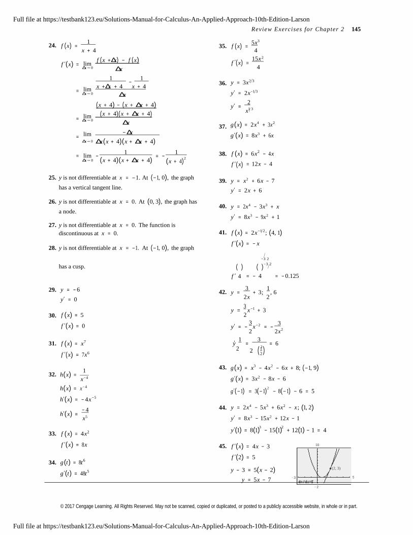
© 2017 Cengage Learning. All Rights Reserved. May not be scanned, copied or duplicated, or posted to a publicly accessible website, in whole or in part.
′ (1 )
− 3 5
Review Exer cis e s for Chapter 2 145
24.
f (x) = 1
35. ( ) 5x 3
x + 4 f x =
4 2
f ′(x) =
=
=
=
lim Δx → 0
lim Δx → 0
lim Δx → 0
lim
f ( x +Δx) − f ( x) Δ x
1 −
1 x +Δx + 4 x + 4
Δ x
( x + 4) − ( x + Δ x + 4) ( x + 4)( x + Δ x + 4)
Δ x
−Δx
36.
37.
f ′(x) = 15x
4
y = 3x2 3
y′ = 2x−1 3
y′ = 2 x1 3
g (x) = 2x4 + 3x2
g′(x) = 8x3 + 6 xΔx → 0 Δ x(x + 4)(x + Δ x + 4)
= lim Δx → 0
− 1
= − 1
(x + 4)(x + Δ x + 4) (x + 4)2
38. f (x) = 6x2 − 4x
( ) f ′ x = 12x − 4
25. y is not differentiable at x = −1. At (−1, 0), the graph
has a vertical tangent line.
26. y is not differentiable at x = 0. At (0, 3), the graph has
a node.
27. y is not differentiable at x = 0. The function is
discontinuous at x = 0.
28. y is not differentiable at x = −1. At (−1, 0), the graph
39.
40.
41.
y = x2 + 6x − 7
y′ = 2x + 6
y = 2 x4 − 3x3 + x
y′ = 8x3 − 9 x2 + 1
f (x) = 2x−1 2 ; (4, 1)
f ′(x) = − x
−3 2
has a cusp. ( ) ( )−3 2
f ′ 4 = − 4 = − 0.125
29.
y = − 6 42.
y = 3
+ 3; 1
, 6
y′ = 0 2x 2
30.
f (x) = 5
f ′(x) = 0
y = 3
x−1 + 3 2
y′ 3
x− 2
3
31.
f (x) = x7
= − = − 2 2 x2
y 1
= 3
= 6
f ′( x) = 7 x6
2 2 2
2
32.
h(x) =
1
x− 4
43. g (x) = x3 − 4x2 − 6x + 8; (−1, 9)
g′(x) = 3x2 − 8x − 6
h(x) = x− 4
h′(x) = − 4 x−5
44.
g′(−1) = 3(−1)2
− 8(−1) − 6 = 5
y = 2 x4 − 5x3 + 6 x2 − x ; (1, 2)h′(x) =
− 4
x5
y′ = 8x3 − 15x2 + 12 x − 1
3 2
33. f (x) = 4x2
y′(1) = 8(1) − 15(1) + 12(1) − 1 = 4
34.
f ′(x) = 8x
g(t) = 8t 6
g′(t) = 48t 5
45. f ′(x) = 4x − 3
f ′(2) = 5
y − 3 = 5(x − 2)
10
(2, 3)
y = 5x − 7 − 2
Full file at https://testbank123.eu/Solutions-Manual-for-Calculus-An-Applied-Approach-10th-Edition-Larson
Full file at https://testbank123.eu/Solutions-Manual-for-Calculus-An-Applied-Approach-10th-Edition-Larson
© 2017 Cengage Learning. All Rights Reserved. May not be scanned, copied or duplicated, or posted to a publicly accessible website, in whole or in part.
x −
146 Chapte r 2 Dif ferentiat i on
46. y′ = 44x3 − 10x 20 50. N = 0.2083t 4 − 7.954t 3 + 11.96t 2 − 706.5t + 3891
y′(−1) = −34
y − 7 = −34(x + 1)
(− 1, 7)
dN =
dt
N ′(t ) =
0.8332t 3 − 23.862t 2 + 23.92t − 706.5
y = −34x − 27 − 2
(a) 2010: N ′(10) = m ≈ − 2020.33
0
− 2 2012: N ′(12) = m ≈ − 2415.85
47. f (x) = x − 1
= x1 2 − x−1 2
x
(b) Results should be similar.
(c) The slope shows the rate at which the number of
f ′(x) = 1
x−1 2 + 1
x−3 2
2 2
1 1 = + 2
farms was increasing or decreasing in that particular
year, or value of t.
In 2010, the number of farms was decreasing about2 x
f ′(1) = 1
2x3 2
− 1
2020.33 thousand per year, and in 2012, the number
of farms was decreasing about 2415.85 thousand
3 per year.y − 0 = 1(x − 1)
y = x − 1
(1, 0)
− 2
51.
f (t ) = 4t + 3; [− 3, 1]
Average rate of change:
48. f (x) = 3 x − x = x1 3 − x f (1) − f (− 3)
1 − (− 3) 7 − (− 9)
= = 4 4
f ′(x) = 1
x− 2 3 − 1 = 1
− 1 3 3 3 x2
f ′(−8) = 1
− 1 = 1
− 1 = − 11
Instantaneous rate of change:
f ′(t ) = 4
3 3 (−8)2
y − 6 = − 11
(x + 8) 12
y − 6 = − 11
x − 22
12 12 f ′(1) = 4
f ′(− 3) = 4
52. ( ) [ ]12 3
f x = x2 + 3x − 4; 0, 1
f (1) − f (0)
0 − (− 4)
11 4 y = −
12 3
Average rate of change: = = 4 1 − 0 1
−10
8
(−8, 6)
3
Instantaneous rate of change:
f ′(x) = 2x + 3
f ′(1) = 5
f ′(0) = 3
49.
−4
R = − 0. 5972t 3 + 51.187t 2 − 485.54t +
2199.0
53. f (x) = x2 3; [1, 8] Average rate of change:
f (8)− f (1)
= 4 − 1
= 3
dR =
dt R′(t ) = −1.7916t 2 + 102.374t − 485.54
8 − 1 7 7
Instantaneous rate of change:
(a) 2008: R′(8) = m ≈ 218.8
2010: R′(10) = m ≈ 359.0
(b) Results should be similar.
(c) The slope shows the rate at which sales were
increasing or decreasing in that particular year,
or value of t.
In 2008, the revenue was increasing about $218.8
million per year, and in 2010, revenue
was increasing about $359.0 million per year.
f ′(x) = 2 3x1 3
f ′(8) = 1 3
f ′(1) = 2 3
Full file at https://testbank123.eu/Solutions-Manual-for-Calculus-An-Applied-Approach-10th-Edition-Larson
Full file at https://testbank123.eu/Solutions-Manual-for-Calculus-An-Applied-Approach-10th-Edition-Larson
© 2017 Cengage Learning. All Rights Reserved. May not be scanned, copied or duplicated, or posted to a publicly accessible website, in whole or in part.
(
Review Exer cis e s for Chapter 2 147
54. f (x) = x3 − x2 + 3; [− 2, 2]
f (2)− f (− 2) Average rate of change: =
2 − (− 2)
7 − (− 9) = 4
4
Instantaneous rate of change: f ′(x) = 3x2 − 2x
f ′(2) = 8
f ′(− 2) = 16
55. s(t ) = −16t 2 − 30t + 600
(a) Average velocity = s(3)− s(1)
= 366 − 554
= −94 ft sec
(b)
(c)
3 − 1 2
v(t ) = s′(t) = −32t − 30
v(1) = − 62 ft sec
v(3) = −126 ft sec
s(t ) = 0
−16t 2 − 30 + 600 = 0
16t 2 + 30t − 600 = 0
−(30) ±
(30)2
− 4(16)(− 600)
− 30 ± 39,300
t = = 2(16) 32
(d)
t ≈ 5.26 sec
v(t ) = s′(5.26) = −32(5.26) − 30 = −198.32 ft sec
56. (a) s(t ) = −16t 2 + 276 58. C = 24,000 + 450 x − x2 , 0 ≤ x ≤ 225
v(t ) = s′(t) = − 32t
dC = 450 − 2x
dx
(b) Average velocity = s(2)− 2(0)
2 − 0 59.
C = 370 + 2.55
x = 370 + 2.25x1 2
= 212 − 276
2
dC
= 1 (2.55) x
dx 2
−1 2 ) = 1.275
x
(c)
v(t) = − 32t
= − 32 ft sec 60.
C = 475 + 5.25x2 3
v(2) = − 64 ft sec dC
= 2
5.25 x−1 3 =
3.5
v(3) = − 96 ft sec dx 3
3 x
(d) s(t ) = 0 61. R = 150x − 0.6x2
−16t 2 + 276 = 0 dR
= 150 − 1.2x dx
16t 2 = 276
t 2 = 276
16
62. R = 150 x − 3
x2
4
(e)
t ≈ 4.15 sec
v(4.15) = −132.8 ft sec
dR = 150 −
3 x
dx 2
57.
C = 2500 + 320 x
63.
R = − 4x3 + 2 x2 + 100x
dRdC = 320
dx
= −12 x2 + 4x + 100 dx
Full file at https://testbank123.eu/Solutions-Manual-for-Calculus-An-Applied-Approach-10th-Edition-Larson
Full file at https://testbank123.eu/Solutions-Manual-for-Calculus-An-Applied-Approach-10th-Edition-Larson
© 2017 Cengage Learning. All Rights Reserved. May not be scanned, copied or duplicated, or posted to a publicly accessible website, in whole or in part.
2
2
148 Chapte r 2 Dif ferentiat i on
64. R = 4x + 10 x1 2 69. f (x) = x3 (5 − 3x2 ) = 5x3 − 3x5
dR = 4 +
5 f ′(x) = 15x2 − 15x4 = 15x2 (1 − x2 )
65.
dx x1 2
P = − 0.0002x3 + 6x2 − x − 2000
70.
Simple Power Rule
f (x) = 4x2 (2x2 − 5) = 8x4 − 20 x2
66.
dP = −0.0006x2 + 12 x − 1
dx
P 1
x3 + 4000 x2 − 120 x − 144,000
f ′(x) = 32 x3 − 40x = 8x(4x2 − 5)
Simple Power Rule= −
15
dP 1 x2 + 8000 x − 120
71. ( )( )
= − dx 5 y = 4x − 3 x3 − 2x2
67. P = − 0.05x2 + 20 x − 1000
(a) Find dP
when x = 100. dx
y′ = (4x − 3)(3x2 − 4x) + 4(x3 − 2 x2 ) = 12x3 − 25x2 + 12 x + 4 x3 − 8x2
= 16x3 − 33x2 + 12x
Product Rule and Simple Power RuledP
= − 0.1x + 20 = P′(x) dx
72.
s = 4 −
1 (t 2 − 3t) = (4 − t −2 )(t 2 − 3t)
t 2
When x = 100, dP dx
= P′(100) = $10.
s′ = (4 − t −2 )(2t − 3) + (t 2 − 3t )(2t −3 )
(b) Find Δ P
for 100 ≤ x ≤ 101. Δ x
= 8t − 12 − 2t −1 + 3t −2 + 2t −1 − 6t −2
= 8t − 12 − 3t −2
P(101) − P(100) 101 − 100
= 509.95 − 500 = $9.95 Product Rule and Simple Power Rule
68.
(c) Parts (a) and (b) differ by only $0.05.
P = − 0.021t 2 + 2.77t + 148.9
73. g (x) = x
x + 3
g′(x) = ( x + 3)(1)− x(1)
(a) P(0) = 148.9
P(4) = 159.644
P(8) = 169.716
g′(x) = (x
(x + 3)
3
+ 3)2
P(12) = 179.116 Quotient Rule and Simple Power Rule
P(16) = 187.844
P(20) = 195.9
74. f (x) = 2 − 5 x
3x + 1
P(23) = 201.501
These values are the populations in millions for
f ′(x) = (3x + 1)(− 5) − (2 − 5x)(3)
(3x + 1)2
−15x − 5 − 6 + 15xBrazil from 1990 to 2013. f ′(x) =
(3x + 1)2
(b) dP
= − 0.042t + 2.77 = P′(t ) dt
f ′(x) = − 11
(c) P′(0) = 2.77
P′(4) = 2.602
P′(8) = 2.434
P′(12) = 2.266
P′(16) = 2.098
P′(20) = 1.93
P′(23) = 1.804
These are the rates at which the population of Brazil
is changing in millions per year from 1990 to 2013.
(3x + 1)
Quotient Rule and Simple Power Rule
Full file at https://testbank123.eu/Solutions-Manual-for-Calculus-An-Applied-Approach-10th-Edition-Larson
Full file at https://testbank123.eu/Solutions-Manual-for-Calculus-An-Applied-Approach-10th-Edition-Larson
© 2017 Cengage Learning. All Rights Reserved. May not be scanned, copied or duplicated, or posted to a publicly accessible website, in whole or in part.
4
2 −5
)
−1 2
2 2
2
5
4
x
=
2
2 (
2
2
2
2
Review Exer cis e s for Chapter 2 149
6 x − 5
6
2 − 4
75. f (x) =
x2 + 1 ̀80. g (x) =
(3x2
− 5x) = 6(3x − 5x)
f (x) ( x + 1)(6)− (6 x − 5)(2 x)
( ) ( )( 2
) ( )′ g′ x 2
2
= 6 − 4 3x − 5x 6x − 5
( + 1) 24(6 x − 5)
x
6 + 10 x − 6 x2
= − 5
3x2 − 5x
=
(x2
+ 1) ( )
General Power Rule
2(3+ 5x − 3x2 )=
(x2 + 1) 81. g (x) = x x
1 2 2 + 1 = x x2 + 1
1 2
−1 2
2
1 2
Quotient Rule and Simple Power Rule g′(x) = x (x 2
+ 1) (2x) + (1)(x
+ 1)
x2 + x − 1
= x2 + 1 x2 +
x2 + 1
76. f (x) =
x2 − 1 ( )
2x2 + 1
( )
f (x) = ( x − 1)(2 x + 1) − ( x + x − 1)(2 x) =
x2 + 1′
( 2 − 1)
Product and General Power Rule
x
2 x3 + x2 − 2x − 1 − 2 x3 − 2 x2 + 2x=
(x2 − 1)
82. g (t ) = t
(1 − t )3
− x2 − 1 x2 + 1=
2 = −
2 3 2
2 2(x − 1) (x − 1) g′(t ) = (1 − t ) (1) − t(3)(1 − t ) (−1)
(1 − t )
6
Quotient Rule and Simple Power Rule (1 − t )
3 + 3t (1 − t )
2
=f x =
3
5x2 + 2 (1 − t )6
77. ( ) ( )
2 2
(1 − t ) + 3t
= =
2t + 1
f ′(x) = 3(5x + 2) (10 x) (1 − t )4
(1 − t )4
= 30 x(5x2 + 2)
Quotient Rule and General Power Rule
General Power Rule
3 2 2
1 3
83.
f (x) = x(1 − 4x2 )78. f (x) = x − 1 = (x − 1)
f ′(x) = x(2)(1 − 4 x2 )(−8x) + (1 − 4x2 )f ′ x
1 −2 3
= x2 − 1 2x 2 x
= 2
79.
( ) ( ) ( ) 2 3 3 3(x2 − 1)
General Power Rule
h(x) = 2
= 2(x + 1)−1 2
= −16 x2 (1 − 4 x2 ) + (1 − 4x2 ) = (1 − 4 x2 )−16x2 + (1 − 4x2 )
( )( )
= 1 − 4 x2 1 − 20x2
x + 1
h′(x) = 2 − 1
(x + 1)−3 2
Product and General Power Rule
5
2
1
84. f (x) = x2 +
1
x = (x2 + x−1 )
5
= − 4
(x + 1)3 2
f ′(x) = 5(x2 + x−1 ) (2 x − x−2 )
General Power Rule
= x2 +
1 2x −
1
x2
Full file at https://testbank123.eu/Solutions-Manual-for-Calculus-An-Applied-Approach-10th-Edition-Larson
Full file at https://testbank123.eu/Solutions-Manual-for-Calculus-An-Applied-Approach-10th-Edition-Larson
© 2017 Cengage Learning. All Rights Reserved. May not be scanned, copied or duplicated, or posted to a publicly accessible website, in whole or in part.
General Power Rule
Full file at https://testbank123.eu/Solutions-Manual-for-Calculus-An-Applied-Approach-10th-Edition-Larson
Full file at https://testbank123.eu/Solutions-Manual-for-Calculus-An-Applied-Approach-10th-Edition-Larson
© 2017 Cengage Learning. All Rights Reserved. May not be scanned, copied or duplicated, or posted to a publicly accessible website, in whole or in part.
4
3 2
3
2 )
2
2
2
4
4
4
4
3
150 Chapte r 2 Dif ferentiat i on
85. h(x) = x2 (2x + 3) = x6 (2 x + 3)3 87. f (x) = x2 (x − 1)
5
2 4 5
h′(x) = x6 3(2 x + 3)2 (2) + 6x5 (2x + 3)
3
f ′(x) = 5x (x − 1) 4
+ 2x(x − 1)
= 6 x5 (2 x + 3)2 x + (2 x + 3)
= 18x5 (2 x + 3)2 (x + 1)
Product and General Power Rule
= x(x − 1) 5x + 2(x − 1)
= x(x − 1) (7 x − 2)
Product and General Power Rule
86.
f (x) = (x − 2)(x + 4)
88. f (s) = s3 (s2
3 5
5 2
− 1
2 3 2
2 2
5 2
f ′(x) = 2(x − 2)(x + 4) (x − 2) + (x + 4)f ′(s) = s ( 2 )(s − 1) (2s) + 3s (s − 1)
= 2(x − 2)(x + 4)(2 x + 2) = s2 (s 2
− 1) 3 2
5s 2 + 3(s2
− 1)
= 4(x − 2)(x + 4)(x + 1)
Product and General Power Rule
= s2 (s 2 − 1) (8s2 − 3)
Product and General Power Rule
89. h(t) =
3t + 1
(1 − 3t )2
2
(3t + 1)1
2
= (1 − 3t)
2
−1 2 1 2
h′(t) = (1 − 3t ) (1 2)(3t + 1) (3)− (3t + 1) (2)(1 − 3t )(−3)
(1 − 3t )4
(3t + 1)−1 2
(1 − 3t )(3 2) + (3t + 1)6=
(1 − 3t )3
3(9t + 5) =
2 3t + 1(1 − 3t )3
Quotient and General Power Rule
90.
g (x) =
3x + 1 (3x + 1) 2
= x + 1 (x2
+ 1)2
2 2 2
g′(x) = ( x + 1) (2)(3x + 1)(3) − (3x + 1) 2( x + 1)2 x
(x2 + 1)
2 2 2 2
6( x + 1) (3x + 1) − 4 x(3x + 1) ( x + 1)=
(x2 + 1)
2(3x + 1)(x2 + 1)3(x2 + 1) − 2 x(3x + 1)=
(x2 + 1)
2(3x + 1)( x2 + 1)(− 3x2 − 2 x + 3)=
(x2 + 1)
2(3x + 1)(− 3x2 − 2 x + 3)=
(x2 + 1)
Quotient and General Power Rule.
Full file at https://testbank123.eu/Solutions-Manual-for-Calculus-An-Applied-Approach-10th-Edition-Larson
Full file at https://testbank123.eu/Solutions-Manual-for-Calculus-An-Applied-Approach-10th-Edition-Larson
© 2017 Cengage Learning. All Rights Reserved. May not be scanned, copied or duplicated, or posted to a publicly accessible website, in whole or in part.
= − 4
= −
= −
= −
2
2
2
2
= )
2
4
Review Exer cis e s for Chapter 2 151
91. T 1300
2 = 1300(t 2
−1
+ 2t + 25
95. f ′′′(x) 3
= −3x− 4
t + 2t + 25
2 −2
x
f (4) (x) = 12x−5T ′(t) = −1300(t + 2t + 25) (2t + 2)
2600(t + 1) f (5) (x) = −60x−6
= −
(t 2 + 2t + 25)
f (6) (x) = 360x−7
= 360 x7
(a) T ′(1) 325
≈ − 6.63°F hr 49
96.
f (x) =
x = x1 2
T ′(3) 13
≈ − 6.5°F hr 2
T ′(5) 13
≈ − 4.33°F hr
f ′(x) =
f ′′(x)
1 x−1 2
2
1 x−3 2
= − = − 3
T ′(10) 1144 841
≈ −1.36°F hr f ′′′(x) =
3 x
8
−5 2
(b) f (4) (x)
15 x−7 2
15
60 = − = − 16 16x7 2
0 24
0
97. f ′(x) = 8x5 2
f ′′(x) = 20x3 2
f ′′′(x) = 30 x1 2
The rate of decrease is approaching zero.
92. When L = 12,
f (4) (x) = 15x−1 2 = 15 x1 2
V = L
(D − 4)2
= 12
(D − 4)2
= 3 (D − 4)
2 98. f ′′(x) = 9 3 x = 9x1 3
16 16 4
dV =
3 (D − 4).
dD 2
f ′′′(x) = 3x− 2 3
f (4) (x) = − 2x− 5 3
f (5) (x) =
10 x−8 3 =
10
(a) When D = 8, dV dD
= 3
(8 − 4) = 6 board ft in.
3 3x8 3
(b) When D = 16,
99. f (x) = x2 + 3 x
= x2 + 3x−1
dV =
3 (16 − 4) = 18 board ft in.
dD f ′(x) = 2 x − 3x−2
(c) When D = 24, f ′′(x) = 2 + 6x−3 = 2 +
6 x3
dV =
3 (24 − 4) = 30 board ft in.
dD
100.
f ′′′(x) = 20 x4 − 2
= 20 x4 − 2x−3
(d) When D = 36, x3
f (4) (x) = 80 x3 + 6 x−4dV =
3 (36 − 4) = 48 board ft in.
dD
f (5) (x) = 240x2 − 24x−5
= 240 x2 − 24 x5
93. f (x) = 3x2 + 7 x + 1
f ′(x) = 6x + 7
f ′′(x) = 6
94. f ′(x) = 5x4 − 6x2 + 2 x
f ′′(x) = 20x3 − 12x + 2
f ′′′(x) = 60 x2 − 12 = 12(5x2 − 1)
Full file at https://testbank123.eu/Solutions-Manual-for-Calculus-An-Applied-Approach-10th-Edition-Larson
Full file at https://testbank123.eu/Solutions-Manual-for-Calculus-An-Applied-Approach-10th-Edition-Larson
© 2017 Cengage Learning. All Rights Reserved. May not be scanned, copied or duplicated, or posted to a publicly accessible website, in whole or in part.
( )
x +
152 Chapte r 2 Dif ferentiat i on
101. (a) s(t ) = −16t 2 + 5t + 30
v(t ) = s′(t ) = − 32t + 5
107. y 2
2 y dy
= x − y
= 1 − dy
a(t ) = v′(t ) = s′′(t ) = − 32 dx dx
(b)
(c)
s(t) = 0 = −16t 2 + 5t + 30
Using the Quadratic Formula, t ≈ 1.534 seconds.
v(t) = s′(t) = −32t + 5
2 y dy
+ dy
= 1 dx dx
(2 y + 1) dy
= 1 dx
dy 1
v(1.534) ≈ − 44.09 ft sec =
dx 2 y + 1
(d) a(t ) = v′(t ) = −32 ft sec2
At (2, 1), dy
dx
= 1
. 3
102. s(t ) = 1
= (t + 1)−2
t 2 + 2t + 1
v(t ) = s′(t ) = −2(t + 1)−3
= − 2
(t + 1)3
y − 1 = 1(x − 2)
3
y = 1
x + 1
3 3
a(t ) = v′(t ) = 6(t + 1)−4
6 =
(t + 1)4
108.
2x1 3 + 3 y1 2
2 x−2 3 +
3 y −1 2
dy
= 10
= 0
103. x2 + 3xy + y3
2 x + 3x dy
+ 3 y + 3 y 2 dy
dx dx
= 10
= 0
3 2 dx
dy
dx
dy
4 y1 2
= − 9x2 3
2dy
3x + 3 y 2 = −2x − 3 y dx
At (8, 4), dx
= − . 9
dy =
−2 x − 3 y
dx 3x + 3 y 2
104. x2 + 9 xy + y 2 = 0
2 x + 3 y = −
3(x + y 2 ) y − 4 = −
2 (x − 8)
9
y 2 52 = − 9 9
2 x + 9 y + 9x dy
+ 2 y dy
dx dx
(9x + 2 y) dy
dx
= 0
= −2x − 9 y
109.
y 2 − 2 x = xy
2 y dy
− 2 = x dy
+ y dx dx
dydy
= −2 x − 9 y
dx 9x + 2 y
2 x + 9 y = −
9 x + 2 y (2 y − x) =
dx y + 2
105.
y 2 − x2 + 8x − 9 y − 1 = 0
dy y + 2 =
dx 2 y − x
2 y dy
− 2x + 8 − 9 dy
= 0 dx dx
At (1, 2), dy
dx =
4.
3
(2 y − 9) dy
dx
= 2 x − 8
y − 2 = 4 (x − 1)
3
dy =
2 x − 8 dx 2 y − 9
y = 4
x + 2
3 3
106. y 2 + x2 − 6 y − 2x − 5 = 0
2 y dy
+ 2x − 6 dy
− 2 = 0 dx dx
dy
(2 y − 6) = 2 − 2 x dx
dy =
2 − 2 x
dx 2 y − 6 =
1 − x
y − 3
Full file at https://testbank123.eu/Solutions-Manual-for-Calculus-An-Applied-Approach-10th-Edition-Larson
Full file at https://testbank123.eu/Solutions-Manual-for-Calculus-An-Applied-Approach-10th-Edition-Larson
© 2017 Cengage Learning. All Rights Reserved. May not be scanned, copied or duplicated, or posted to a publicly accessible website, in whole or in part.
( )
Review Exer cis e s for Chapter 2 153
110. y3 − 2 x2 y + 3xy 2
3 y 2 dy − 2x2 dy
− 4 xy + 6 xy dy
+ 3 y 2
dx dx dx
= −1
= 0
dy 3 y 2 − 2x2 + 6xy = 4xy − 3 y 2
dx
At (0, −1), dy
dx
= −1.
dy =
dx
4 xy − 3 y 2
3 y2 − 2x2 + 6 xy
y + 1 = −1(x − 0)
y = − x − 1
111. A = π r 2
dA dr = 2π r
dt dt
113. Let b be the horizontal distance of the water and h be the
depth of the water at the deep end.
Then b = 8h for 0 ≤ h ≤ 5.
V = 1 bh 20
= 10bh = 10 8h h = 80h2
(a) Find dA
when r = 3 in. and dr = 2 in. min.
( ) ( ) 2
dt dt
dV dhdA
= 2π (3)(2) = 12π in.2 min = 160h
dt dtdt dh
1 dV 1 1≈ 37.7 in.2 min
= dt 160h dt
= (10) = 160h 16h
(b) Find dA
when r = 10 in. and dr
= 2 in. min. When h = 4, dh
= 1
= 1
ft min.dt dt dt 16(4) 64
dA = 2π (10)(2) = 40π in.2 min
dt
114.
P = R − C
112.
P = 375x − 1.5x2
≈ 125.7 in.2 min = xp − C
= x(211 − 0.002x) − (30 x + 1,500,000)
= 181x − 0.002x2 − 1,500,000dP
= 375 dx
− 3.0x dx
dP dx dxdt dt dt = 181 − 0.004 x
dP = (375 − 3.0x)
dx dt dt dt
dP dxdt dt = (181 − 0.004x)
dt dt
(a)
(b)
dP = 375 − 3.0(50)(2) = $450 day
dt
dP = 375 − 3.0(100)(2) = $150 day
dt
dP = 181 − 0.004(1600)(15) = $2619 week
dt
Full file at https://testbank123.eu/Solutions-Manual-for-Calculus-An-Applied-Approach-10th-Edition-Larson
Full file at https://testbank123.eu/Solutions-Manual-for-Calculus-An-Applied-Approach-10th-Edition-Larson
© 2017 Cengage Learning. All Rights Reserved. May not be scanned, copied or duplicated, or posted to a publicly accessible website, in whole or in part.
1 2
2
154 Chapte r 2 Dif ferentiat i on
Chapter 2 Test Yourself
1. f (x) = x2 + 3; (3, 12) 7. f (x) = (x + 3)(x2 + 2 x)
f ′(x) = f ( x +Δx) − f ( x) lim f (x) = x3 + 5x2 + 6xΔx → 0
= lim
Δx → 0
Δx
( x +Δx)2
+ 3 − ( x2 + 3) Δx
f ′(x) = 3x2 + 10 x + 6
(Or use the Product Rule.)
= lim
Δx → 0
x2 + 2 xΔx + (Δx)2
+ 3 − ( x2 + 3) Δx
8. f (x) = x (5 + x) = 5x1 2 + x3 2
5 3 5 3 x
2 xΔx + (Δx)2
f ′(x) = x
+ x = +
= lim Δx → 0 Δx
−1 2 1 2
2 2 2 x 2
= lim
Δx 2 x + (Δx) 9. f (x) = (3x2 + 4)
Δx → 0 Δx f ′(x) = 2(3x2 + 4)(6 x)= lim 2x + Δx
Δx → 0
= 36 x3 + 48x= 2 x
At (3, 12): m = 2(3) = 6
10.
f (x) =
1 − 2x
= (1 − 2x)
f ′ x 1 −1 2
= 1 − 2x −22. f (x) = x − 2; (4, 0)
( ) ( ) ( ) 2
1f ′(x) =
lim Δx → 0
f ( x +Δx) − f ( x) Δx
x +Δx − 2 − ( x − 2)
= − 1 − 2x
3
= lim (5x − 1)
f x =Δx → 0
= lim
Δx → 0
= lim
Δx
x +Δx − x
Δx
1
11. ( )
f ′(x) =
x
x(3)(5 x − 1)2 (5) − (5x − 1)
3
x2
( )2 ( )
Δx → 0
= 1
x + Δx + x 5x − 1
= 15x −
x2
5x − 1
2 x = (5x − 1)
2 (10 x + 1)
x2
At (4, 0): m = 1
= 1
2 4 4
3. f (t ) = t 3 + 2t
12. f (x) = x −
1 4
x
f ′ x
= 1 + 1
f ′(t) = 3t 2 + 2 ( )
x2 − 6
6
(1, 0)
4. f (x) = 4 x2 − 8x + 1 f ′(1) = 1 +
1 = 2
12
− 4
f ′(x) = 8x − 8
5. f (x) = x3 2 + 6x1 2
y − 0 = 2(x − 1)
y = 2 x − 2
f ′(x) =
3 x1 2 + 3x−1 2
= 3 x
+ 3
2 2 x
6. f (x) = 5x2 − 3
= 5x2 − 3x−3
x3
f ′(x) = 10 + 9x− 4 = 10 x +
9 x4
Full file at https://testbank123.eu/Solutions-Manual-for-Calculus-An-Applied-Approach-10th-Edition-Larson
Full file at https://testbank123.eu/Solutions-Manual-for-Calculus-An-Applied-Approach-10th-Edition-Larson