c©Copyright 2014

Miro Enev

Machine Learning Based Attacks and Defenses in Computer Security:Towards Privacy and Utility Balance in Sensor Environments

Miro Enev

A dissertationsubmitted in partial fulfillment of the

requirements for the degree of

Doctor of Philosophy

University of Washington

2014

Reading Committee:

Tadayoshi Kohno, Chair

Shwetak Patel

Dieter Fox

Program Authorized to Offer Degree:Department of Computer Science and Engineering

University of Washington

Abstract

Machine Learning Based Attacks and Defenses in Computer Security: Towards Privacyand Utility Balance in Sensor Environments

Miro Enev

Chair of the Supervisory Committee:Associate Professor Tadayoshi KohnoComputer Science and Engineering

The growth of smart devices and the Internet of Things (IoT) is driving data markets in

which users exchange sensor streams for services. In most current data exchange models,

service providers offer their functionality to users who opt-in to sharing the entirety of the

available sensor data (i.e., maximal data harvesting).

Motivated by the unexplored risks in emerging smart sensing technologies this disser-

tation applies the lens of machine learning to understand (1) to what degree information

leakage can be exploited for privacy attacks and (2) how can can we go about mitigating

privacy risks while still enabling utility and innovation in sensor contexts.

In the first part of this work, we experimentally investigate the potential to amplify

information leakage to unlock unwanted [potentially harmful] inferences in the following

emerging technologies:

• smart homes – we show that electromagnetic noise on the powerline can be used to

determine what is being watched on TVs.

• smart cars – messages between sensors and control units can be used to determine

the unique identity of the driver.

We use the insights gained from these investigations to develop a theoretical balanc-

ing framework (SensorSift) which provides algorithmic guarantees to mitigate the risks of

information sharing while still enabling useful functionality to be extracted from the data.

SensorSift acts as a data clearing house which applies transformations to the sensor

stream such that the output simultaneously (1) minimizes the potential for accurate infer-

ence of data attributes defined as private [by the user], while (2) maximizing the inferences

about application requested attributes verified to be non-private (public).

We evaluate SensorSift in the context of automated face understanding and show that

it is possible to successfully create diverse policies which selectively hide and reveal visual

attributes in a public dataset of celebrity face images (i.e., prevent inference of race and

gender while enabling inference of smiling).

Through our work we hope to offer a more equitable balance between producer and

consumer interests in sensor data markets by enabling quantitatively provable privacy con-

tracts which (1) allow flexible user values to be expressed (and certifiably upheld), while

(2) simultaneously allowing for innovation from service providers by supporting unforeseen

inferences for non-private attributes.

Stepping back, in this dissertation we have identified the potential for machine inference

to amplify data leakage in sensor contexts and have provided one direction for mitigating

information risks through theoretical balance of utility and privacy.

TABLE OF CONTENTS

Page

Chapter 1: Introduction . . . . . . . . . . . . . . . . . . . . . . . . . . . . . . . . . 1

1.1 Vision and Goal . . . . . . . . . . . . . . . . . . . . . . . . . . . . . . . . . . 2

1.2 Contributions . . . . . . . . . . . . . . . . . . . . . . . . . . . . . . . . . . . . 2

Chapter 2: Related Work and Technical Background . . . . . . . . . . . . . . . . . 6

2.1 Adversarial Inferences . . . . . . . . . . . . . . . . . . . . . . . . . . . . . . . 6

2.2 Utility Privacy Balance in Sensor Contexts . . . . . . . . . . . . . . . . . . . 7

2.3 Methods and Evaluation . . . . . . . . . . . . . . . . . . . . . . . . . . . . . . 8

Chapter 3: TV EMI . . . . . . . . . . . . . . . . . . . . . . . . . . . . . . . . . . . 11

3.1 Introduction . . . . . . . . . . . . . . . . . . . . . . . . . . . . . . . . . . . . . 11

3.2 Background and Related Work . . . . . . . . . . . . . . . . . . . . . . . . . . 13

3.3 Experimental Methods . . . . . . . . . . . . . . . . . . . . . . . . . . . . . . . 18

3.4 Analysis Methods . . . . . . . . . . . . . . . . . . . . . . . . . . . . . . . . . . 23

3.5 Results . . . . . . . . . . . . . . . . . . . . . . . . . . . . . . . . . . . . . . . . 24

3.6 Discussion . . . . . . . . . . . . . . . . . . . . . . . . . . . . . . . . . . . . . . 30

3.7 Summary . . . . . . . . . . . . . . . . . . . . . . . . . . . . . . . . . . . . . . 32

Chapter 4: Driver Fingerprinting – Unique Identification from Vehicle Sensor Data 33

4.1 Introduction . . . . . . . . . . . . . . . . . . . . . . . . . . . . . . . . . . . . . 33

4.2 Related Work . . . . . . . . . . . . . . . . . . . . . . . . . . . . . . . . . . . . 37

4.3 Threat Model . . . . . . . . . . . . . . . . . . . . . . . . . . . . . . . . . . . . 40

4.4 Background . . . . . . . . . . . . . . . . . . . . . . . . . . . . . . . . . . . . . 41

4.5 Experimental Data Collection . . . . . . . . . . . . . . . . . . . . . . . . . . . 44

4.6 Analysis Methods . . . . . . . . . . . . . . . . . . . . . . . . . . . . . . . . . . 49

4.7 Results . . . . . . . . . . . . . . . . . . . . . . . . . . . . . . . . . . . . . . . . 54

4.8 Discussion . . . . . . . . . . . . . . . . . . . . . . . . . . . . . . . . . . . . . . 62

4.9 Conclusion . . . . . . . . . . . . . . . . . . . . . . . . . . . . . . . . . . . . . 66

4.10 Acknowledgments . . . . . . . . . . . . . . . . . . . . . . . . . . . . . . . . . . 67

i

Chapter 5: SensorSift: Balancing Sensor Data Privacy and Utility . . . . . . . . . 68

5.1 Introduction . . . . . . . . . . . . . . . . . . . . . . . . . . . . . . . . . . . . . 68

5.2 Background and Related Work . . . . . . . . . . . . . . . . . . . . . . . . . . 71

5.3 System Description . . . . . . . . . . . . . . . . . . . . . . . . . . . . . . . . . 72

5.4 Analysis Methods . . . . . . . . . . . . . . . . . . . . . . . . . . . . . . . . . . 77

5.5 Experimental Methods . . . . . . . . . . . . . . . . . . . . . . . . . . . . . . . 80

5.6 Results . . . . . . . . . . . . . . . . . . . . . . . . . . . . . . . . . . . . . . . . 86

5.7 Discussion . . . . . . . . . . . . . . . . . . . . . . . . . . . . . . . . . . . . . . 93

5.8 Acknowledgments . . . . . . . . . . . . . . . . . . . . . . . . . . . . . . . . . . 94

Chapter 6: Conclusion . . . . . . . . . . . . . . . . . . . . . . . . . . . . . . . . . . 95

Bibliography . . . . . . . . . . . . . . . . . . . . . . . . . . . . . . . . . . . . . . . . . 97

ii

ACKNOWLEDGMENTS

I would like to thank Prof. Tadayoshi Kohno for his wisdom and guidance through

difficult academic terrain. He has taught me much about leadership and scholarship and I

hope to continue learning from him as a lifelong friend!

I would also like to express my gratitude to my thesis committee, research collaborators,

and the students in the Security and Privacy Lab who have inspired and assisted me in

realizing the various components of my doctoral work.

Lastly, I would like to thank my family and friends whose unfaltering love and support

provided me with the strength needed to reach my goals.

iii

1

Chapter 1

INTRODUCTION

Participatory sensing scenarios are those in which individuals send along their sensor

data streams to 3rd parties in exchange for services. Such data exchanges are increasing

in frequency, and are part of a growing market that enables: optimization of energy con-

sumption in homes/Internet of Things (e.g., Google Nest, Belkin Echo); insurance pricing

models based on behavior in cars (e.g., Progressive Snapshot, StateFarm Pay-as-you-Drive);

tracking of fitness goals via worn devices (e.g, Fitbit, Jawbone); and gesture recognition in

homes and public settings (e.g., Microsoft Kinect, Google Glass).

The services provided in exchange for data continue to improve through entrepreneurial

effort, and in most instances, smart sensor applications create rewarding experiences and

assistive services. However, the gathered raw data also presents significant privacy risks in

the form of:

• full disclosure of sensor data – most opt-in privacy contracts maximize the data

that the service provider gathers (even when this is not critical for desired function-

ality) [1, 2, 3].

• multiple layers of misuse possibilities – the data can be compromised or inter-

cepted by an adversary before it leaves the user’s device (e.g, malware exfiltration), it

can be compromised anywhere along the communication path to the service provider

(e.g., man-in-the middle), or it could be compromised once in possession of an up-

stream receiver.

• long lived risks – the conclusions drawn from the data can be connected with medical

or health factors that have privacy implications for the entire lifetime of a targeted

individual.

2

Thus we argue that even if applications are trustworthy, it is important to realize that

the data can be misused anytime along the connectivity chain and its storage life-cycle and

hence privacy defenses must be improved.

1.1 Vision and Goal

In our present work we seek to understand the potential for privacy risks in emerging sensor

technology contexts. We also attempt to develop methods to empower stakeholders with

tools to better control their information releases. Specifically, we explore the impact of

mitigating risks at the time of information release as a way to deal with the utility and

privacy tension inherent in current data sharing scenarios.

We focus on machine learning (ML) as an evaluation framework because we hypothesize

that ML will be utilized by well intentioned and adversarial processors of sensor data. This

belief is premised on the strong synergy created by sensor data fueled by machine learning

algorithms; in particular, machine learning methods offer theoretical guarantees to improve

task performance with additional experience (more data) and sensor data streams offer a

plentiful source of very rich data signals (often continuous and high dimensional).

1.2 Contributions

1.2.1 Attacks and Risk Analysis

We begin by applying machine learning to investigate the potential for adversarial inference

with several attacks based on sensor streams. In particular, we focus on two case studies that

represent different points in the spectrum of future technologies; we pick these two examples

because homes and cars provide coverage of key spaces in which sensor data streams are

likely to include private aspects of human activity.

• homes - where we extract 1-dimensional electromagnetic interference (EMI) signa-

tures from televisions, and

• cars - where we extract 16-dimensional signals from messages passed between vehicle

sensors and control units.

3

In our work with TV EMI we show how a single easy to install plug-in device can infer

the content of what is being watched on television by simply monitoring the electrical noise

generated by the TV’s power supply. We show that given a 5-minute recording of the

electrical noise of a DVD movie, we can accurately determine which was being shown by

matching query data to a database of noise signatures. In addition, we demonstrate this

phenomenon in real homes despite the presence of noise from other electrical devices.

In the vehicular context, our results also indicate high potential for privacy breaking

attacks as we demonstrate that drivers have unique fingerprints which are captured in

snippets of sensor data collected during natural driving behavior. Specifically, we find that

it is possible to recognize the operator of a vehicle (among a set of 15 candidate drivers)

with 100% accuracy using a training and test database that uses multiple sensor streams

collected over a 15-minute period. When longer datasets are available, high identification

accuracy turns out to be possible using a single sensor (e.g., the most telling is the brake

pedal position).

The combined results from our attack studies reinforce our initial hypothesis that ma-

chine learning can amplify the risks of information leakage, and hence, further support our

stance towards sharing only the minimum data necessary in participatory sensor scenarios.

1.2.2 Defense Strategy Design and Implementation

To better prepare future data stakeholders for navigating emerging sensor data-sharing

opportunities we develop an algorithmic defense framework that empowers an alternate

exchange mechanism where users define what attributes (or inference) in the data they con-

sider private and release sifted (algorithmically transformed) versions of their data streams

where (i) private attributes are unrecognizable to machine classifiers while (ii) non-private

attributes can still be correctly identified by service providers.

We evaluate this framework (called SensorSift) in the context of very rich sensor streams

– static and dynamic camera images (> 1000 dimensions per sample) – and investigate the

potential to use machine classifiers to recognize visually describable characteristics about

faces in a public dataset of celebrity images. We find that we can create sifts that provide

4

strong privacy and minimize utility losses at (K = 5 dimensions) for the majority of policies

we tested (average PubLoss = 6.49 and PrivLoss = 5.17, see Chapter 5 for details). We

were able to find high performing sifts for various policies which include several public and/or

several private attributes (e.g., hide race and gender while enabling detection of smiling) and

also show high performance in video data (e.g., streaming images) in an extension study.

Our results indicate that it is possible to empower users and service providers to enter

into a quantitatively provable privacy contracts 1 which allow (1) flexible user values to be

expressed (and upheld), while simultaneously (2) supporting innovation by enabling requests

by 3rd-parties for future [unforseen] aspects of the data.

While we recognize that there are limitations of our contribution (see Chapter 5), we

hope that this dissertation provides insights for novel technical directions in balancing utility

and privacy in emerging technology contexts.

1.2.3 Summary

In this work we sought to analyze the information privacy risks emerging in sensor contexts

and to also explore potential defenses. We were motivated towards this line of research

because service providers in sensor data-sharing scenarios currently dictate too much of the

information ecosystem; in particular, we feel that consumers (participating stakeholders)

have too little control with regard to how much data is collected, how its processed, and

how it is stored.

In the Chapters 3 and 4 of this dissertation, we emphasize the importance of minimizing

the amount of information released to 3rd-parties in exchange for services because task-

irrelevant data (information leakage) can be misused for privacy breaking inferences using

machine learning methods. These chapters experimentally investigate the attacks possible

using sensor data extracted from home and car settings and show that it is possible to

determine (1) what is being watched on a television from electromagnetic noise on the

powerline, and (2) that the driver of a vehicle can be recognized from the sensor data

flowing through the vehicle’s internal communication network.

1Using ensembles of modern machine classifiers as benchmarks for privacy and utility of sifted data.

5

Subsequently, in Chapter 5 we develop a sifting algorithm which offers a technical defense

mechanism for balancing utility and privacy in sensor data sharing settings. We evaluate

this algorithm in the context of automated face understanding and show that it is possible

to defend user defined [private] attributes from machine inference while enabling accurate

classification of non-private attributes requested by service providers.

Our contribution is thus twofold. First, we experimentally demonstrate the power of

machine learning to amplify information leakage in emerging sensor contexts. Second, we

develop a data transformation method which can be used in a quantitative clearinghouse to

enable safer information exchanges in which users are empowered to flexibly express their

privacy values while still releasing data from which service providers can extract utility.

6

Chapter 2

RELATED WORK AND TECHNICAL BACKGROUND

Below we summarize past work in data privacy risks and defenses and highlight the

high level differences between our contributions and past work. We also provide a brief

background about the technical components shared between our studies and leave the unique

technical details in each of the subsequent chapters.

2.1 Adversarial Inferences

The computer security literature has long been fascinated with information leakage through

non-obvious channels. Although not brought to the public’s attention until 1985 [4], evi-

dence suggests that the government have long known that ancillary electromagnetic emis-

sions from CRT devices can leak private information about what those devices might be

displaying [5, 6]. This early work on studying electromagnetic information leakage from

CRTs has since been extended to flat-panel displays [7] and wired and wireless keyboards

[8].

More recently, Marquardt et al. showed that smartphone accelerometers can infer more

than input occurring on the phone. They developed (sp)iphone that collected accelerometer

readings while the smartphone is placed next to a keyboard [9]. The vibrations of a user

typing on the keyboard is recorded by the phone and generally interpreted to predict what

was typed. This technique is similar to acoustic keyboard side-channels that use audio

recordings to learn user input [10, 11] as well as keystroke timing techniques [12].

Focusing on powerlines, Clark et al. demonstrated that it is possible to infer what

webpage is being visited using measurements of AC consumption with an instrumented

outlet [13]. Their classifier was able to reach 99% precision and 99% accuracy in matching

9,240 web page loads (15 seconds each) amongst a set of 50 candidate websites.

Both the new and previous results should be considered conservative estimates of the

7

potential threats. Enhancements in unsupervised feature extraction, larger data sources,

and the rise of multimodal sensors will likely lead to greater delity side channels as has been

already demonstrated in [10, 11]. There are many other examples which we do not cite here

but encourage interested readers to seek out the latest literature surveys in cyberphysical

security and information privacy especially in sensor and ubiquitous computing settings

(such as [14] and [15]).

2.2 Utility Privacy Balance in Sensor Contexts

In the context of data disclosure with simultaneous privacy and utility constraints the

framework of k-anonymity was suggested as a strong candidate mechanism. K-anonymity

protection of a data disclosure is met if the information for each individual (table row)

cannot be distinguished from at least k − 1 other individuals in the released data. The set

of the individual in question and the k − 1 records form an equivalence class (the records

are indistinguishable from each other). A stronger version of k-anonymity is l-diversity;

l-diversity requires that each equivalence class has at least l well-represented values for each

sensitive attribute (an attribute is a column, and a sensitive attribute is a column that

carries information capable of uniquely identifying a row). The strongest notion of privacy

is t-closeness, which requires that the distribution of a sensitive attribute in any equivalence

class is close to the distribution of the attribute in the overall data (i.e., the distance between

the subset and the largest distribution should be no more than a threshold t) [16, 17, 18].

If the goal of a database is to summarize aggregate statistics about its constituents

(statistical utility) while revealing none of their personal data, then differential privacy is

the mechanism of choice. A database satises differential privacy if the addition or removal of

a single database element does not change the probability of the outputs to identical queries

by more than some small amount. The denition is intended to capture the notion that being

able to query the total distribution is informative about aggregate trends but not informative

about any specific individual. Individuals may submit their personal information to the

database secure in the knowledge that (almost) nothing can be discovered from the database

with their data added that could not have been discovered without their data. [19, 20].

In the context of sensor systems the problems of balancing utility and privacy are usu-

8

ally focused on privacy-preserving transformations of the sensor data so as to minimize

policy-defined private information leakage while retaining data aspects necessary for util-

ity extraction. In such settings the theoretical tools which apply to statistical databases

or large releases of equivalence classes do not apply. The dynamic demands of the sensor

setting also rule out the use of using homomorphic cryptosystems (two parties can suc-

cessfully carry out a computation without either party being aware of the constituents of

the computation) which are either somewhat efficient (yet only partially homomorphic), or

fully homomorphic and, at present, vastly inefficient [21]. Somewhat more pertinent are

the systems based approaches which typically use proxies/brokers for uploading user gen-

erated content prior to sharing with 3rd-parties. These approaches use access control lists,

privacy rule recommendation, and trace audit functions; while they help frame key design

principles, they do not provide quantitative obfuscation algorithms beyond degradation of

information resolution (typically for location data) [22].

SensorSift (see Chapter 5), in contrast to the statistical or identity-focused privacy

approaches described above, offers a more granular level of privacy analysis which is suited

to dynamic/interactive smart sensing contexts. Unlike identity information, attributes can

be used to track the dynamic state of the user (e.g., mood, energy level, social engagement).

Furthermore, since attributes are properties that transcend the specific task at hand, they

can be learned once and then applied to novel contexts without the need for a new training

phase (‘zero-shot’ transfer learning [23]).

2.3 Methods and Evaluation

In much of this thesis work we perform case studies of experimental information privacy

analysis using supervised learning. We have applied supervised learning to analyze the po-

tential for information privacy breaches in several sensor contexts. In contrast, when focused

on developing information privacy defenses we have used supervised learning to establish

that privacy-preserving transformations produce outputs which allow inferences on all but

a set of private data attributes. We introduce the shared components of the methodological

structure below as it provides a common framing for the forthcoming discussions of the

work we have completed.

9

2.3.1 Supervised Learning

Supervised learning is the machine learning task of inferring a mapping from input objects

(i.e., feature vectors of raw data samples) to target outputs (i.e., categories) using training

data to choose the optimal mapping. The name supervised learning is fitting because the

training data includes numerous data instances paired with their corresponding desired out-

put value (supervisory signal). Once stable performance has been reached on the training

data set, the trained model is evaluated on unseen data to evaluate generalization perfor-

mance. The accuracy achieved during this generalization, or test phase, is the ultimate

fitness criterion for the model.

2.3.2 Formal Setup

More explicitly the setup of a supervised learning task follows the following structure:

• Data Preparation - Pairs of input objects and target labels are gathered for a given

problem setting by performing experiments or accessing public data. Depending on

the state of the input it is often necessary to perform additional pre-processing steps

such as resampling, normalization, denoising, smoothing, or filtering.

• Extract features - Next features are defined over the pre-processed inputs. This can

be done in a supervised fashion by an investigator who chooses a suitable representa-

tion given domain knowledge. Alternative it can be accomplished using unsupervised

methods which extract pattern dictionaries which capture the underlying structure of

the training data. It is also possible to have a combination of supervised and unsu-

pervised (a.k.a., semi-supervised) methods which offer the potential benefits of both

approaches. Lastly in cases where the dimensionality of the inputs is impractical for

computation, dimensionality reduction techniques can be used to compress the data

prior to feature selection without significant impact on performance.

• Transform Data* - (*Optional) In the case of defensive frameworks, there is typ-

ically a data transformation that occurs which intends to minimize any information

10

orthogonal to the goal of the problem. There are various techniques for achieving this

objective including noise injection, data removal, and pseudonymization. Additional

details are available in the related work section.

• Choose Learning Model(s) - At this stage of the process, the investigator selects

an algorithm to apply to the learning task. Popular methods include support vector

machines, random forests, neural networks, and decision trees. We prefer to use an

ensemble of such methods for greater coverage of the learning model hypothesis space.

When multiple methods are used in unison it is important to develop a voting scheme

to aggregate responses or to select the response of the model with highest confidence.

• Training Phase - Before the start of training, the available labeled data is usually

divided into a training set (typically >= 80% of the data) and a testing set (the

remaining non-training data). The testing set is then further sub-divided into com-

plementary subsets for cross-validation rounds. One round of cross-validation involves

performing the analysis on one subset (of the training data, thus a subsubset of the

original data), and validating the analysis on the other subset. To reduce variability,

multiple rounds of cross-validation are performed using different partitions, and the

validation results are averaged over the rounds. Cross-validation is useful to maximize

the potential of the learning phase by finding the model that generalizes best across

the training data. Different learning algorithms have different rules for training, how-

ever they are all usually run until parameters converge to a stable point or until the

maximum amount of iterations (or total running time ) is exceeded. At this point the

learning stage is complete.

• Testing and Evaluation Phase - Lastly, the learned model is checked on its ability

to generalize beyond what it has seen in training and correctly predict the labels from

the data in the test set. This is the performance criteria reported by the investigator

and usually takes the form of classification accuracy computed as the ratio of correct

predictions relative to the total number of test cases.

11

Chapter 3

TV EMI

3.1 Introduction

In this chapter we begin our investigation of the privacy attacks possible using information

leakage, and specifically focus on sensors data collected from the electrical infrastructure

of a connected/smart home. There is already a growing concern that a home’s power con-

sumption data could reveal private information about the occupants’ personal activities.

Indeed, the Electronic Frontier Foundation (EFF) recently submitted a request to the Cal-

ifornia Public Utilities Commission, to petition the adoption of stronger laws to protect

sensitive energy consumption data [24, 8]. EFF’s motivation for the policy change is based

on discoveries revealing that power consumption information can be used to recognize “the

use of most major home appliances” and more alarmingly to track “sleep, work, and travel

habits” [24].

The EFF’s claims are backed by recent findings that power consumption data can be

used to infer appliances use. The rapidly evolving research strand of electrical sensing has

reached a high level of specificity showing that it is possible to tell the difference between

multiple devices used in a home simultaneously (by analyzing their unique noise signatures

over the powerline) [25, 26]. The principal goal of prior research in electrical sensing has

been to aid users in adopting efficient energy habits and for developing activity recognition

applications. As an example of a possible use case, consider a home monitoring device

which determines that every evening between 8-10pm a single-occupant homeowner leaves

the lights on in her bedroom and bathroom while watching TV in the living room. Having

reached this conclusion the device informs the homeowner of the monetary benefits of turn-

ing off those unutilized lights and reducing her energy footprint. Such an advanced level of

energy tracking and inference also enables numerous other applications which correlate con-

sumption to activity. For example, the activation of a series of lights and electrical devices

12

can help determine one’s path or location within the home to aid in elder care by allowing

a remote caretaker to assess the amount and nature of activity [27].

While such monitoring devices have the potential to increase efficiency and lead to

quality of life improvements, the underlying methods are clearly unsettling when viewed

through a privacy lens. Unfortunately, a privacy-centric security analysis has been lacking

in the energy sensing community which has thus far been exclusively focused on developing

novel technologies while helping people become more conscientious consumers. As part of

the attack component of this dissertation (see Chapter 1), we seek to flip this situation

around and asks: how much information can one learn from monitoring a home’s power

line infrastructure? Is the electrical signal used for tracking consumption also capable of

revealing private activity data? Said another way: are currently unknown forms of sensitive

information leaking out over our power lines, waiting to be discovered?

To examine this question thoroughly, we have chosen to study the power-line information

leakage due to the incidental electromagnetic noise generated from a single class of home

appliances: televisions (TVs). We chose to focus on TVs because they are a nearly ubiqui-

tous, high-end technology. Past research has shown that it is possible to detect when a TV

is operating in a home [25, 26]; but could the electromagnetic noise from a TV’s switching

power supply leak information beyond its on/off power state? We find that the answer is

a definitive yes! Moreover, we show that given a 5 minute recording of the electrical noise

unintentionally produced by the TV it is possible to infer exactly what someone is watching

by matching it to a database of content signatures (96% average classification success in a

database of 20 movies). Notably, our method requires only one sensor which can be installed

anywhere along the powerline (i.e., does not require installing a power monitor in-line with

the electrical power source of the home or the device of interest).

Given the potential exposure of sensitive information over the powerline, a natural next

step would be to asses the privacy risks faced by modern homeowners. We address this

question more deeply in the body of the chapter, but stress several important points below.

Firstly, there are already natural entities capable of mounting the attacks we expose.

For example, a power company with a modern smart power meter can remotely collect

sufficient information to mount an attack. Moreover, anyone capable of attaching a device

13

to a home’s powerline would be able to mount this attack (e.g., a parent wishing to track a

child’s TV viewing habits when the parent is not home, a neighbor plugging a device into

an external power outlet, or the manufacturer of a Trojan appliance like a picture frame

with wireless capabilities to exfiltrate data).

In addition to the attack scenarios of today, we conjecture that (1) future appliances may

leak even more information over the powerline (a conjecture we support in the discussion

sections of this chapter given recent power efficiency mandates like Energy Star), and (2) as

future homes become increasingly networked, new measurement vectors are likely to appear

over time.

Lastly, there are serious challenges in developing defense mechanisms against information

leakage, because a tension begins to develop between the need for more energy efficient

devices and preserving one’s privacy. For the remainder of the chapter, we begin with a

discussion of relevant prior work and go on to present the key concepts needed to understand

the information leakage phenomenon over the powerline. Next we shift our focus to detailing

the experimental data collection and analysis workflow necessary to infer TV content from

electrical noise. We then briefly sketch several motivating examples of threat models. In

the last two sections we describe a theoretical model that can learn to mimic the electrical

noise produced by a TV and conclude with a discussion of the universality of our approach,

possible obfuscation mechanisms, and interesting security challenges.

3.2 Background and Related Work

3.2.1 Related Work

Evidence suggests that the government have long known that ancillary electromagnetic

emissions from CRT devices can leak private information about what those devices might

be displaying [5, 6]. This early work on studying electromagnetic information leakage from

CRTs has since been extended to flat-panel displays [7] and wired and wireless keyboards

[8]. The principal differences between this prior work and our own is that all the prior

work uses electromagnetic interference that is emitted, that is, it travels through air and

can be picked up wirelessly over a short range. Our work uses conducted electromagnetic

14

interference which propagates from the device over to the power lines of a home.

Related to power consumption, but slightly further afield, is the broader area of power

analysis and differential analysis for cryptographic processors [28]. Other examples of in-

formation leakage vectors include the time to perform various tasks (e.g., [29]), optical

emanations (e.g., [30] for network appliances and [31] for CRTs), acoustic emanations (e.g.,

for printers [32], CPUs [33], and keyboards [34]), and reflections (e.g., [35]). In the modern

television space, past work has also shown that it is possible to infer what someone might

be watching over a wireless video stream from the size of the transmitted packets [36]; that

approach exploits information leakage through variable bitrate encoding schemes, which was

concurrently pioneered in [37].

Detecting electrical device activity and power consumption in the home has gener-

ally been done in the ’distributed sensing model’ wherein each device being monitored

is equipped with a separate sensor. This one sensor per device model is limiting because as

the name suggests each monitored device requires separate instrumentation. Researchers in

the ubiquitous computing field have been trying to use a single sensor approach in the home

to infer human activity from the incidental noise produced by devices in the home as their

signal. Gupta et al. accomplished this by using a single sensor that can be plugged into any

available electrical outlet and analyzing the conducted electromagnetic interference (EMI)

present on the powerline in the frequency domain [25]. In this transformed space different

devices occupy different frequency ranges centered around the switching frequencies of their

power supplies. The presence or absence of such EMI is a direct consequence of the on or off

state of a device respectively. In this work, we leverage the same fundamental phenomenon

but move beyond detecting the power state of a device to infer the content being shown on

the screen.

3.2.2 Theory of Operation

In this section we describe the fundamental theory behind the powerline information leakage

phenomenon which is made possible by unintentional electrical noise production in modern

appliances. We also highlight the pros and cons of alternative methods that can provide

15

access to the same information source.

EMI

The drive to produce smaller, cheaper and more efficient consumer electronics has made

the use of Switched Mode Power Supplies (SMPS) increasingly prevalent. The adoption of

SMPS is also spurred by policy guidelines as manufacturers strive to provide products which

meet the efficiency requirements set by the Department of Energy’s Energy Star program. In

contrast to linear power regulation based supplies, SMPS do not dissipate excess energy as

heat but rather store it in the magnetic field of an inductor. The load output of the inductor

can be modulated by using a switch that allows current to flow when the circuit is closed

(switch is on); thus by modulating the opening and closing of the switch the circuit is able

to regulate the amount of power output. In modern SMPS this modulation, also known as

the ’switching frequency,’ happens at a very high rate (typically tens to hundreds of KHz).

A side effect of an SMPS’s operation is that the modulation of the inductor’s magnetic

field produces large amounts of unintentional electromagnetic interference (EMI) centered

at and around the switching frequency. Due to the physical contact between the powerline

and the device this EMI gets coupled onto the powerline, which then propagates the noise

throughout the entire electrical infrastructure of a home. This is known as conducted EMI.

Because such EMI is undesired, in the US, the Federal Communications Commission (FCC)

sets rules for any device that connects to the powerline and limits the amount of EMI it can

conduct (47CFR part 15/18 Consumer Emission Limits). This limit is set to -40dBm for a

frequency range between 150 KHz to 500 KHz (which is much higher than the lowest levels

of EMI that our prototype system can sense and capture effectively -100dBm). Figure 3.1

shows the EMI as captured by our system for various devices in a home. These include a

compact fluorescent lamp (CFL), a modern LCD television, and other SMPS based devices.

Modern high definition liquid crystal display (LCD) televisions, which are of particular

interest to our study, dominate today’s consumer market and are almost always based on

switched mode power supplies. As a result, the majority of modern TVs have power supplies

that produce unintentional EMI. We implemented a system that records this signal [25] and

16

Figure 3.1: Frequency domain Waterfall plot of the EMI spectrum in a home (red = highamplitude signal, blue = low amplitude). Note the dynamic nature of the TV EMI from 60KHz (dark scene/low power consumption) to 90 KHz (bright scene/high power consump-tion). Interesting events for other devices are labeled numerically 1: Washer Spin CycleLeft, 2: Off, 3: Spin Right 4: CFL Light ON, 5: OFF, 6: ON

in our experiments, we found that the TV produces a static band of EMI centered at the

switching frequency of the SMPS. Furthermore we observed that the switching frequency

(and EMI band) can be translated by altering the brightness setting of the television. Even

more interesting is that the dynamic video content on the TV screen produces fluctuations

in the EMI which leads to a time varying signal that fluctuates in a +/− 20 KHz window

centered at the switching frequency (Figure 3.1). To better understand this phenomenon,

we used an inline power sensor to determine the consumption of the TV in real time. We

observed two things. First, that the power consumption changes as a function of the screen

brightness (menu setting), and second, that it also fluctuates as a function of change in

screen content.

To summarize, the brightness menu setting of the TV determines the baseline power

consumption of the device, and changing this setting requires the SMPS to alter its switching

frequency to match the load. In addition the dynamic visual content on the screen causes

systematic fluctuations around this baseline since darker images require less energy while

lighter screen content requires more. These content driven consumption changes manifest

themselves as fluctuations in the EMI (which to reiterate, is an artifact of the SMPS’s

adjustments to match the power draw). In the case of our Sharp 42” LCD TV, changes in

17

brightness setting cause the center frequency of the EMI to be translated between 65 KHz

and 75 KHz while modulating screen content cause the EMI to sway around this center

(between 60 KHz and 90 KHz). In the analysis that follows, we use the time varying EMI

as a source of information about on screen-content and track this feature to determine what

is being watched.

Current Consumption as a Feature

As described above, the power consumption of the TV is modulated by the nature of the

dynamic screen content. Because power is the product of voltage and current, screen content

changes should be manifested as changes in the amount of current that the TV draws. To

validate this hypothesis, we collected current consumption data alongside the EMI trace

and found the signals to be identical; suggesting the validity of either approach for inferring

the contents on a TV screen. Though the current consumption data carries information

about screen content, it comes with its own disadvantages in that current sensors have to

be installed ’in line’ with the TV. Ideally this means the sensor is attached to the power

cord of the TV itself, or alternatively is instrumented inside the breaker panel. If the latter

of these options is chosen, the sensor would also be reporting the current draw from all other

devices in the home. Such an additive mixture of current consumption greatly complicates

the isolation of the TV’s signal. In contrast, the voltage EMI approach offers greater

flexibility as it relies on a voltage sensor which could be plugged into any electrical outlet in

the home. Moreover our EMI collection technique utilizes frequency domain analysis which

allows us to simultaneously track multiple devices with low probability of signal clutter.

Proof of Plausibility

To use EMI as a tool for inferring what is watched on a TV we needed to ensure that

multiple recordings of the same visual inputs led to repeatable EMI signals while differing

video content produced dissimilar EMI traces. To test whether these conditions were met we

recorded data from four movies (60 minutes of data per movie) and repeated the recording

three times (for a total of 3 recording sessions).

18

Figure 3.2: Figure 2. Repeated recordings of identical screen content lead to nearly equiv-alent EMI traces (Panels A vs. B, Lion King, correlation = .989), while content fromdifferent movies produces distinct electrical noise patterns (B vs. C; Lion King vs. BourneUltimatum, correlation = .402).

Next we analyzed the cross-correlation of the same movie between sessions and found

that the similarity was consistently over 98% in all possible session pairings. This finding

validated our requirement for signal consistency and the result is visually apparent in the

top two panels (A, and B) of Figure 3.2, which represent 7 minutes of sample data from

two recordings of the same movie (The Lion King).

When different movies are compared, the amount of cross correlation between their EMI

signal traces is a function of the similarity of their content. Panel C of Figure 3.2 depicts

a 7 minute trace from The Bourne Ultimatum which is apparently different from the data

recorded from The Lion King (Panels A and B).

3.3 Experimental Methods

Our early experiments convinced us that there exists a strong relationship between EMI

and screen content and that we had a sufficient platform to derive an algorithm capable

of matching EMI traces from sections of movies to a film database in order to infer what

is being watched. The next step was to build a recording setup that captures EMI from

multiple movies, processes the signal, and populates a database with the EMI trace. We

expected to process a large number of movies (multiple times) so we opted to create an

automated data collection environment to guarantee consistency across recording sessions.

19

Figure 3.3: Recording Hardware Setup. S = Spectrum Analyzer, P = powerline Interface(PLI), U = Universal Software Radio (USRP), I = Isolating Transformer. The Sharp 42”LCD TV and the data logging PC are also visible.

3.3.1 Hardware and Signal Processing

Our prototype consists of three main components (Figure 3.3). First, we connect a powerline

interface module (PLI) to any electrical outlet of the recording environment to gather the

conducted EMI signal. Second, a high speed data acquisition module is used to digitize the

incoming analog signals from the PLI. Lastly, a data collection and analysis PC running

our custom software conditions and processes the incoming signals from the digitizer. We

also connect a spectrum analyzer for debugging purposes and for visualizing the real-time

EMI signal as a waterfall plot.

Of the components we use for data collection the only custom hardware is found within

the PLI. The analog frontend PLI module is essentially a voltage sensor with a high pass

filter that removes the AC line frequency (60 Hz in the US). This is necessary so that

the dynamic range of the digitizer and the spectrum analyzer are not overwhelmed by the

strong amplitude of the 60 Hz carrier wave and its harmonics (including the hazardous 120V

output). The PLI’s high-pass filter has a flat frequency response from 50 KHz to 30 MHz,

20

allowing us to capture the entire range of conducted EMI. The analog signal from the PLI

is then fed into a USRP (Universal Software Radio Peripheral) which acts as a high speed

digitizer. We set the sampling rate of the USRP to 500 KHz, which (under the Nyquist

Theorem) allows us to effectively analyze the spectrum from 0 to 250 KHz. The digitized

data from the USRP is then streamed in real time over a USB connection to a PC.

We developed software on the PC which extends upon the GNU Radio Companion

platform. Our system processes the incoming data and performs a real time Fast Fourier

Transform (FFT) on the time domain signal arriving from the USRP. The output of the FFT

is a frequency domain signal (or an FFT vector) of 2048 points which are spread uniformly

over the entire spectral range from 0 to 250 KHz. The FFT vector is computed 122 times

per second and its contents corresponds to the magnitude of the frequency strength along

the range. The stream of FFT vectors is stored on the data recording PC for post-processing

by our feature extraction algorithm. Figure 3.1 depicts a waterfall plot of a sequence of FFT

vectors captured over a 200 second window.

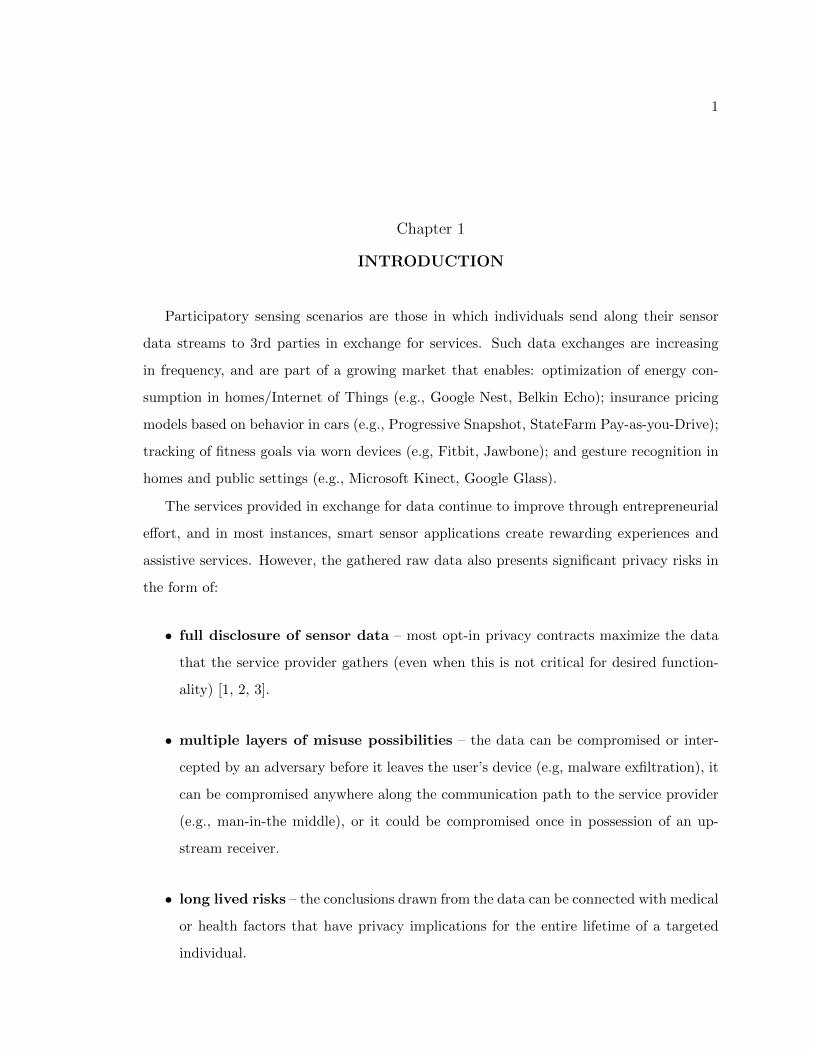
3.3.2 Feature Extraction

Since we are only interested in tracking the TV, we post process the raw FFT bins and

only retain the region around the TV’s central frequency. This means that we reduce the

2048 element vector to 122 points in the 60-90KHz range wherein the EMI signal fluctuates

(Figure 3.4). In order to reduce the dimensionality of the data we perform a decimation

to reduce the rate at which FFT vectors are processed. We found that to capture the

variability in the EMI signal from the TV, using every 40th FFT vector (a decimation

factor of 40) was sufficient. Next we iterate through each time sample of the [abridged] 122

element FFT and extract the maximal element. We do this because we seek to compress the

signal to a single point per time sample. The extracted maxes are then filtered using a 2nd

order low-pass digital Butterworth filter with normalized cutoff frequency of .05 (frequency

where the magnitude response of the filter is (1/2)(1/2)). This removes the oscillation

artifacts in the EMI and yields a smooth timeseries (EMI trace) whose shape tracks the

fluctuations in the raw data (Figure 3.4 - blue overlay). Prior to storing the EMI trace we

21

Figure 3.4: Raw FFT signal around the EMI band of the TV. The result of post-processingthis signal to extract the EMI trace features is overlaid as the blue time series. Note thatunlike Figure 3.1 which also shows raw FFT data, the time axis is now along the horizontal.

perform mean removal (centering) and normalization to capture relative differences around

the center frequency.

3.3.3 Data Collection

To validate our content inference approach, we recorded EMI data during the playback of

20 different movies on a Sharp LC-SB45U LCD 42” TV. At the end of the data collection

our database contained three sessions of recordings (each session contained 20 movies, and

only the first 60 minutes of each movie were considered to ensure data length consistency).

We hypothesized that there may be differences in the EMI features between genres so

we tailored our choices to include 5 genres with 4 representative films per category. Our

selection was informed by genre labels gathered from the internet movie database (IMDB,

imdb.org) and in general we opted to choose titles which spanned a range of years and were

among the most popular in their respective categories (see table below).

For illustrative purposes the first 15 minutes of 4 movie EMI traces are shown in Figure

3.5. Note the elevated level of EMI fluctuation in the Bourne Ultimatum; this is typical

of action movies which have a consistently high rate of scenes changes. Other than this

observation we did not find any statistically significant differences between movie genres in

our database.

22

Table 3.1 Movie Database Contents

Action Lord of the Rings: Return of the King, Star

Wars V: Empire Strikes Back, The Bourne Ul-

timatum, The Matrix

Animation Wall-E, Shrek 2, The Lion King, Aladdin

Comedy Office Space, Meet the Parents, The Hangover,

Wedding Crashers

Documentary Planet Earth: Fresh Waters, Food Inc., An In-

convenient Truth, Top Gear (s.14;ep.7)

Drama The Shawshank Redemption, American Beauty,

Titanic, Requiem for a Dream

Figure 3.5: Selected Movie Traces. From Top To Bottom these are: An Inconvenient Truth,Meet the Parents, Wedding Crashers, The Bourne Ultimatum, and Shrek 2.

23

Lab and Home Data

The three data recording sessions described above were performed in a lab environment.

To demonstrate the applicability of our approach in naturalistic settings, we also recorded

the same 20 movies in three homes. The key difference between the data collection in the

lab and home deployments was the use of a line isolation transformer in the lab setting

(Tripp Lite 250W isolation transformer). A line isolator is essentially a broadband filter

that removes any EMI present on the powerline and presents an EMI free power output

(are often used in audio/video recording studios and other high end applications). In the

lab environment, we plugged the TV and the PLI into the line isolator’s output to ensure

that the PLI would have exclusive access to the EMI from the TV without interference from

other electrical devices. In the naturalistic case, we collected data from the three homes

without the line isolator, and the PLI captured EMI generated from the TV as well as

myriad other devices (power adapters, CFL and dimmer based lighting, appliances etc.). In

some instances, we found devices which generated electrical noise in the same range as the

signal we were tracking (TV’s EMI). As we show in Section 3.5.3, despite such overlaps, the

ability to infer screen content was relatively unhindered.

Automation

We opted to create an automated data collection environment to guarantee consistency

across recording sessions. To this end we created a system which synchronized movie play-

back and data logging. The software running on the PC sent video content to the TV via a

composite connection and simultaneously recorded data samples (computed FFT vectors)

streaming in from the USRP to a binary file for post-processing and analysis.

3.4 Analysis Methods

Once we constructed our database of reference EMI traces we could focus on designing a

search method to find matches given a query trace. We crafted an algorithm that would

take as input a query (snippet from an EMI movie trace), traverse the database, and return

the movie with the highest similarity to the input.

24

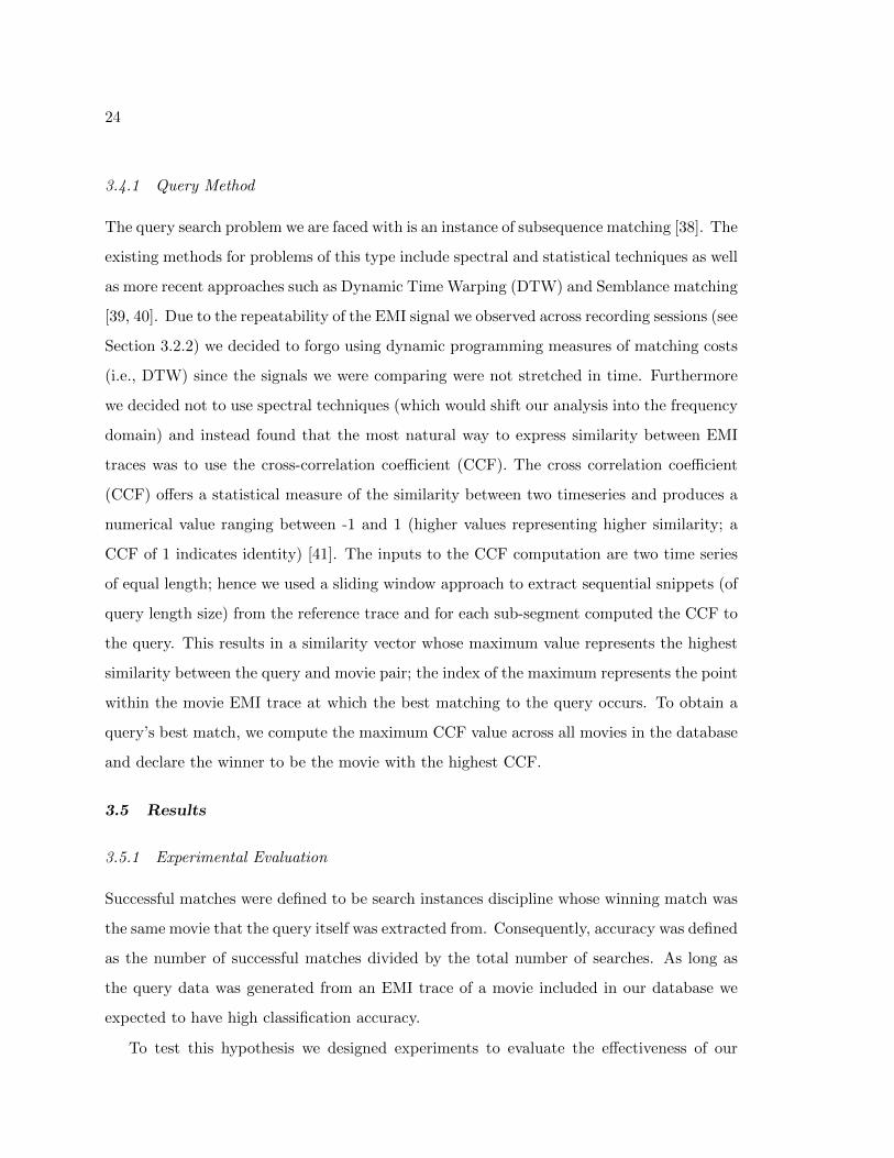
3.4.1 Query Method

The query search problem we are faced with is an instance of subsequence matching [38]. The

existing methods for problems of this type include spectral and statistical techniques as well

as more recent approaches such as Dynamic Time Warping (DTW) and Semblance matching

[39, 40]. Due to the repeatability of the EMI signal we observed across recording sessions (see

Section 3.2.2) we decided to forgo using dynamic programming measures of matching costs

(i.e., DTW) since the signals we were comparing were not stretched in time. Furthermore

we decided not to use spectral techniques (which would shift our analysis into the frequency

domain) and instead found that the most natural way to express similarity between EMI

traces was to use the cross-correlation coefficient (CCF). The cross correlation coefficient

(CCF) offers a statistical measure of the similarity between two timeseries and produces a

numerical value ranging between -1 and 1 (higher values representing higher similarity; a

CCF of 1 indicates identity) [41]. The inputs to the CCF computation are two time series

of equal length; hence we used a sliding window approach to extract sequential snippets (of

query length size) from the reference trace and for each sub-segment computed the CCF to

the query. This results in a similarity vector whose maximum value represents the highest

similarity between the query and movie pair; the index of the maximum represents the point

within the movie EMI trace at which the best matching to the query occurs. To obtain a

query’s best match, we compute the maximum CCF value across all movies in the database

and declare the winner to be the movie with the highest CCF.

3.5 Results

3.5.1 Experimental Evaluation

Successful matches were defined to be search instances discipline whose winning match was

the same movie that the query itself was extracted from. Consequently, accuracy was defined

as the number of successful matches divided by the total number of searches. As long as

the query data was generated from an EMI trace of a movie included in our database we

expected to have high classification accuracy.

To test this hypothesis we designed experiments to evaluate the effectiveness of our

25

Figure 3.6: Accuracy as a function of Query Length. Note that the accuracy improvementsare minimal once the query length reaches 4 minutes (240 s) - indicated by the dashed line.In these home deployments the average accuracy was notably degraded (98% accuracy inlab for a 10 minute query vs 85.8% accuracy in homes). A thorough investigation of ourapproach in naturalistic settings is beyond the scope of the current work yet we feel thatour preliminary study suggests the feasibility of EMI-based content inference in residentialdeployments.

inference algorithm as we varied relevant parameters. We conducted a set of experiments

in which we manipulated the following variables: query length, starting query location, and

combinations of data sources for the query and database.

In order to investigate the effect of query length on accuracy we chose 9 monotonically

increasing query lengths ranging from 15 seconds to 20 minutes (15s, 30s, 60s, 120s, 240s,

300s, 600s, 900s, 1200s). For each query length we generated 10 randomly chosen indexes

(ranging between 0 and 3600 seconds) as query starting locations. Lastly to ensure that

our metric is consistent across recordings we enumerated all possible pairings of sessions for

query and database sources (Query from Session1: DB from Session2 , Q S2: DB S1, Q

S1: DB S3, Q S3: DB S1, Q S2: DB S3, Q S3: DB S2). We then invoked the matching

algorithm once for each possible parameter combination (9 * 10 * 6 = 540 runs).

26

Figure 3.7: Average confusion matrices for selected query lengths for the entire database.Red represent a high level of similarity and blue a low level.

3.5.2 Lab Results

A plot of the average accuracy (across session combinations and query start indexes) as

a function of query length is shown in Figure 3.6. From this curve we can deduce that

even short length queries lead to high accuracy classification. In particular, once the query

length exceeds 4 minutes the accuracy reaches a rate of 95.7% (regardless from which part

of the movie the query segment is chosen). Performance improvements due to extended

query lengths (4 minutes and beyond) do not significantly change the average accuracy but

they do reduce the variability in the results. This can be seen in Figure 3.7 which depicts

averaged confusion matrices for selected query lengths (averaging is done across session

combinations and query start indexes). The diagonal entries represent successful matches.

Note the decrease in the perceived similarity of off-diagonal entries as the query length

increases. Movies 11 (Office Space) and 12 (Meet the Parents) were the worst performers

and we believe that this is due to their consistently high brightness, which produced very

little fluctuation in their EMI traces.

3.5.3 Home Results

Having found convincing results in the lab setting, we were interested in validating our

approach in naturalistic deployments.

We setup our system in three different home environments and in each context recorded

a smaller version of our database. All three homes were in the Seattle area; Home 1 was a

27

Table 3.2 Table 2: Content Classification Accuracy in Homes

Home # Avg. Accuracy

1 93.2%

2 76.4%

3 87.8%

typical suburban house in Lake City, Home 2 was a townhouse in the University District,

and Home 3 was an apartment building in the Green Lake area.

The home data collection consisted of 10 minute segments collected from each of the

20 movies. Using this database we repeated the experiments described in Section 3.3 with

the caveat that we fixed the query length to a 10 minute EMI trace (to exploit the entire

recording from the home). The need for this longer query length was intended to offset the

the increased noise conditions in the homes. The majority of appliances in a home do not

disturb the signal quality of the TV EMI which we track however there are certain devices

which produce obscuring noise (i.e. dimmer switches, washers, and vacuums). We did not

limit the use of these and appliances and asked the residents of the home to ignore the

recording system.

Perhaps of interest is the relationship between the accuracy of the search algorithm and

the number of residents in a home. Homes 1 and 3 are both inhabited by a married couple

whereas in home 2 there are four college house mates . The low accuracy in the more densely

populated home is due to more devices being active on average (i.e. increased probability

of signal pollution in the bands of the EMI spectrum tracked by the inference algorithm).

3.5.4 Learning Models of EMI

Motivated by the robust relationship we found between screen content and EMI we sought

to reverse engineer the method by which electromagnetic noise is produced as a function of

changing video input. Access to this transfer function would allow us to predict the EMI

without actually laying out content on the screen and hence bypass the need for physical

access to the target device. In the following section we investigate the plausibility of finding

28

this function by framing the problem as an instance of supervised learning using a recurrent

neural network with compressed input features.

Input Features

The transfer function we seek to approximate takes in as input a sequence of 3 dimensional

RGB matrices (one per frame) and produces as output a time series of EMI (normalized

between 0:1). The full input matrix is extremely high dimensional ( 106 elements - color R,

G, B* screen width pixels * screen height pixels) and prohibitively large for use in its full

state. Thus we opted to compress each video frame into a 10 element vector which extracts

selected features from the visual content and greatly reduces the complexity of the learning

problem. Since we did not know which aspects of the screen content contribute most to

the EMI signal we chose varied features in hopes that they would be sufficient to drive the

learning. The features we derived from each video frame are as follows:

• brightness: cumulative sum of averaged RGB intensities

• flux: average change in brightness b/w consecutive frames

• edge intensity: cumulative sum of Canny Edge filter output

• FFT: slope of the best fit line to an FFT of the image (the FFT shape becomes nearly

linear after the frequency and amplitude axes are converted using a log-log scale)

• color: mean and standard deviation of fitted gaussians for the R, G, and B color

histograms (6 parameters total)

Neural Network

Since we are dealing with a function fitting problem of unknown complexity, we chose to

use a recurrent neural network (RNN) model in order to accommodate for possible dynamic

and non-linear effects. RNNs are a class of neural networks in which intermediate layers

(i.e. those separating input and output) have connections to neighboring layers as well as

29

Figure 3.8: Neural Net output (red) vs Ground Truth EMI (blue).

(re)connections to themselves; these properties lead to self feedback (i.e. memory) which

enable dynamic temporal behavior [42] At time t the network input layer consisted of a

video frame represented as a 10 element feature vector. The input layer was connected to

the first of 3 hidden layers (connected in succession, each composed of 10 neurons to match

the dimensionality of the input) and the final hidden layer was connected to a scalar output

layer representing the EMI at time t. The training phase began with randomly initialized

network parameters which were tuned using backpropagation through time (BPTT) via the

Levenberg-Marquardt gradient method. The criterion for performance was the how well the

network output matched desired EMI for a given video input (measured as mean squared

normalized error). Each training session concluded when the optimization converged or

after 50 epochs (whichever came first). We ran several hundred training experiments and

chose the network which performed best on sets of test inputs.

Although there is much more that can be done in this line of analysis, our preliminary

results are promising. (Figure 3.8) shows RNN predictions (driven via visual features) vs

actual EMI of a 6 minute trace recorded from the opening segment of Lord of the Rings: The

Two Towers. Though not perfect, the fit above clearly suggests that supervised methods

can be used to train generative models of EMI.

30

3.6 Discussion

Thus far we have shown that modern switched-mode power supplies (SMPS) generate elec-

tromagnetic interference (EMI) which can be measured from a single sensor (anywhere on

the powerline) and produce a high frequency signal which reflecting dynamic changes in

power consumption. Below we address how these findings may extend beyond the TV and

also discuss some of the challenges in defending consumer privacy.

3.6.1 Other TVs and Devices

Although we are only focused on a single TV, our results extend to other televisions and

consumer electronic devices that employ SMPS (DVRs, PCs, power adaptors, CFLs, etc).

The trend towards more efficient Energy Star compliant power supplies is growing (several

states mandate the use of switching power supplies) which suggests an increased potential

for privacy vulnerabilities in the near future.

As we demonstrated earlier in the chapter, different devices exhibit EMI at varying

center frequencies depending on the switching characteristics of the SMPS. The tolerance

in the internal electronics that make up the SMPS can provide enough signal diversity

in the frequency domain to allow multiple [similar] devices to be observed simultaneously.

Depending on the load characteristics of the electronics, the switching frequency can range

from anywhere between a few KHz to 1 MHZ. LCD TVs tend to exhibit similar EMI

behavior between models and brands because they require similar functionally. Newer LED

TVs are also similar to LCDs, but the resonant frequency may be slightly different and the

dynamic nature of the noise may need to be extracted using a different method than the

one we propose (Section 3.5.2). The challenge with tracking new devices, however, is that

they need to be tested to ensure the existence of a strong relationship between EMI and

screen content changes.

The information leakage phenomenon we observe in TVs is likely to hold for many

other consumer electronic devices. Often the power draw of a device can be a strong

indicator of its activity (as has been confirmed in prior work from the security community).

Beyond TVs, another popular class of devices which produce information leakage is home

31

theater audio systems (in these appliances the output volume typically modulates the SMPS

switching frequency). Since hi-end audio receivers typically employ multiple power supplies,

we conjecture that these distinct sources of EMI would produce a richer signal that would

allow for more sophisticated inference into the state of the receiver.

3.6.2 Potential Defenses

There are a number of potential defense mechanisms that could be used to minimize infor-

mation leakage through EMI. The simplest is the use of a powerline isolator similar to the

one used in our laboratory experiments. The internal transformer provides enough isolation

such that the high frequency noise does not pass back over the powerline (assuming the iso-

lator itself has not been comprised). We have observed the isolation phenomenon in some,

but not all, uninterruptable power supplies (UPSs). Most power strips only offer transient

noise suppression and rarely offer any high frequency noise rejection. Notably, some newer

home theater line conditioners, which have a build in power bar, do offer some isolation

capabilities.

A potential whole home solution, which does not require installing a device behind every

electronic appliance, would be to inject random broadband noise over the powerline. The

challenge with this approach is that it must conform to FCC regulations. In addition,

this would cause problems with legitimate powerline-based communication systems like

broadband over powerline and X10 home automatic systems. A more practical could identify

potential devices that may be leaking information by observing the powerline and only

blocking certain frequency bands.

The other defense may be to devise new regulation on how SMPS power supplies are

built. One critical observation, however, is that it may be impossible to fully defend against

such information disclosure while still being in compliance with Energy STAR. Said another

way, government regulation may make it difficult or infeasible to implement defenses since

the costs of privacy (increased consumption and decreased efficiency) are in direct conflict

with recent legislation.

32

3.7 Summary

We have demonstrated that significant information leakage is present in modern switching

power supplies found in many new consumer electronic devices. We have found that a single

easy to install plug-in device can infer the content of what is being watched on television by

simply monitoring the electrical noise generated by the TVs power supply. Only a 5 minute

recording of the electrical noise of a particular movie, is needed to infer the movie from a

database of noise signatures with up to 93% accuracy in actual homes. Although we have

only demonstrated this with TVs, we believe our approach extends to other devices that

employ SMPS. DVD players, power adaptors, and home theater systems all modulate their

power draw during their operation, which can be used to infer its activity.

33

Chapter 4

DRIVER FINGERPRINTING – UNIQUE IDENTIFICATION FROMVEHICLE SENSOR DATA

Building upon our investigation with home sensors and TV content inference, we wanted

to explore the potential for adversarial inference in another emerging sensor context – smart

vehicles. In addition we also wanted to expand our risk analysis beyond the one-dimensional

EMI signal to multi-dimensional continuous sensor data (as is the case with the information

we collect from our experimental vehicle).

4.1 Introduction

Modern vehicles have evolved past their purely mechanical roots into powerful cyber-

physical systems which combine sophisticated sensing, processing, and networking capabili-

ties. These technologies have led to numerous advances in safety, efficiency, and engagement;

however, they have also created novel security and privacy risks as our vehicles transition

into mobile computerized platforms.

4.1.1 Automotive Security

From an automotive security standpoint, significant work has already been done by industry

and the academic community to understand and safeguard against the most likely cyber-

threats.

A recent comprehensive survey of automotive vulnerabilities by Kosher et al. [43] demon-

strated multiple points of entry into the car’s internal communications network from where

researchers could remotely inject malicious messages to compromise and control vehicle

state (e.g., incessant release of washer fluid, disabling dashboard indicators, triggering or

disabling brakes at speed). From this and other work [44, 45, 46] it has become clear

that many of the traditional black-hat hacking methodologies developed in the PC world

34

are translatable to the embedded computing infrastructure of a modern car (e.g., buffer

overflows, packet injection, spoofing/privilege escalation, and botnet-like patching/malware

deployment via command-and-control servers).

Due to the high potential danger to human life from a compromised vehicle, policy

makers and industry leaders have been quick to introduce new national and international

electronic security standards (e.g, SAE, NHSTA, US-CAR); and integrate cyber-physical se-

curity best-practices into the manufacturing of vehicles and vehicle parts (e.g., GM, OnStar,

Intel) [47].

4.1.2 Automotive Privacy

Unlike the unified response towards automotive security threats, there is substantially less

consensus towards the privacy risks emerging alongside the digital evolution of the modern

car.

On one hand, several US states have made it unlawful to access the sensor data of a

vehicle without the permission of the owner and a senate bill (Driver Privacy Act, Hoeven,

Klobuchar, Jan. 14, 2014) has been proposed to enact this legal perspective at the federal

level. On the other hand, more than a million users are already sharing their vehicle’s sensor

streams with a growing market of data consumers.

Although we support the effort towards basic legal protections for data access, these

protections have no practical impact on data exchanges initiated by individuals who opt-in

to sharing their vehicle sensor streams with 3rd-parties such as insurance companies (e.g.,

Progressive’s Snapshot, State Farm’s In-Drive), car manufacturers (e.g., GM, Totota, Tesla,

Volvo, and BMW; efficiency and safety improvements), telematics service providers (e.g.,

OnStar, SYNC, and In-Drive; help and emergency services), and technology start ups (e.g.,

Automatic.com, Kiip.com, moj.io; gameification, targeted ads, and efficiency reporting).

4.1.3 Goal and Motivation

The goal of our current effort is to inform drivers (stakeholders) about the existing in-

formation leakage risks by experimentally measuring the ability to identify the operator

35

of a vehicle (among 15 possible drivers) from segments of sensor streams collected during

approximately 3 hours of natural driving behavior.

Unlike past work which has looked at driving inferences using data from phones, vehicles

with added sensors, or driving simulations, we focus on (1) natural driving data, (2) from

a stock vehicle, and (3) limit our analysis to a subset of 16 basic sensors.

Our test vehicle has between 50 and 80 data streams including a microphone sensor

(for telematics purposes), global positioning system, barometric pressure sensor, and many

others. Although we could have used all of the available data on the internal network for

driver identification, we chose to focus on a subset of basic sensors which we passively logged

without making any modifications. The motivation for our sensor selection was to focus our

analysis on fingerprinting the way the driver dynamically performs actions to control the

vehicle (without added knowledge of external surroundings) using a minimal set of sensors

we expected to be available in most cars on the road today.

Out of the possible inferences to perform, we focus on driver fingerprinting because it has

many interesting properties, and demonstrates the potential for utility benefits and privacy

risks to co-exist in data sharing situations.

From a utility perspective, driver identification can be used to unlock various forms of

useful functionality including: theft prevention, individualized medical emergency response,

efficiency recommendations (suggested adaptations tailored to driver), awareness monitor-

ing (individualized cognitive load tracking), and customized infotainment. Conversely, from

a prviacy perspective the ability to determine the vehicle driver from sensor data could also

have adverse effects such as tracking/surveillance, profiling, incrimination, and bootstrap-

ping other adversarial inferences.

In addition to the utility and privacy implications, driver identification is also compelling

because it is non-subjective and does not depend on an imposed metric (e.g., aggressive-

ness level); and its is fixed over long intervals as driving strategy and execution are

unlikely to change once learned [48, 49].

36

4.1.4 Experimental Database

Existing cars contain numerous computers, many of which are connected to each other

over an internal computer network. Some of these computers broadcast sensor information

over this internal computer network. For our experiments, we connect to the car’s internal

computer network over a federally-mandated port exposed under the dash of every modern

car sold in the U.S. This is the same port that many after-market 3rd-party components

are connected to, e.g., the Progressive Auto Insurance dongle.

To ground our investigation in driver fingerprinting we collected an experimental database

composed of 57.2 hours of sensor data from 15 subjects as they each drove the same vehicle

(2009-edition modern sedan) along the same course consisting of two parts: (1) 3 laps of

parking lot maneuvers, and (2) an open-road 50 mile inter-urban loop spanning various road

types. The total duration of the parking lot data collection was about 7 minutes, and the

open road recording sessions lasted less than 3 hours (average per driver).

4.1.5 Research Questions

Using this dataset, we sought to quantify the potential to identify the driver of a vehicle from

test snippets of driving behavior presented to machine classifiers trained on data from our

subject pool (using 10 way cross-validation, 90% train set, 10% test set). More specifically

we asked the following series of questions:

• Is it possible to distinguish drivers above chance using our experimental setup and all

available data?

• Is it possible to reach accurate identification using a reduced set of sensors, or even a

single sensor?

• Is it possible to accurately identify drivers with limited amounts of training data?

Our results show that it is possible to answer all of these questions affirmatively. In

particular we find that within our dataset:

• 100% driver ID is possible using 15 sensors and the entire database of driving data.

37

• 100% driver ID is possible using a single sensor (brake pedal) and the entire database

for training.

• 100% ID is possible given short training datasets (8 mins, 15 mins, 1 hour) and multiple

sensors; 87% accuracy is achievable using a single sensor (brake pedal) and only the

first 15 minutes of open-road driving as a training database.

These results indicate that differences in driving style are distinguishable using sensor

data from stock vehicle sensors; and that not much data (or many sensors) are needed.

Although we only looked at 15 drivers we believe that this method could scale especially

when multiple non-redundant sensors are chosen and the search is constrained to drivers in

a local area (vs. the entire world population).

Extension: Fingerprint Stability

As an extension we also explored whether a single driver could be consistently identified

across multiple days of data recording and differences in the course.

To this end we selected one driver and collected 5 round trips from the University to

a nearby town (22 mile trip). Using this dataset as a query (and our original dataset as

training) we applied our analytic methods to find that our test driver’s unique fingerprint

was consistent across multiple days and roads (91% accuracy, same driver different roads

and days of data collection).

4.2 Related Work

Past work on driver inferences from sensor data has focused on enabling improvements in

efficiency, safety, and assistive systems. Below we briefly cover several measurement and

behavior adaptation results to provide context for related work in the field. Sections II-

A and II-B can be skimmed for readers interested in the security-focused related works.

In Section II-C we discuss two papers which have also looked at driver identification and

describe the key differences their work and our contribution.

38

4.2.1 Optimizing Infrastructure and Behavior

Early work in driver inference from sensor data was done for the purposes of traffic engi-

neering as Burnham et al. developed control theoretic models to explain behavior patterns

in car-following (spacing relative to forward vehicles) in the mid 1970’s. This work and

much of the subsequent studies for a decade were based on macro measurement datasets

which recorded the trajectories of vehicles along highway road segments (typically urban

crossings) with infrastructure sensors (e.g., video surveillance and loop detectors) [50, 51].

More recent work has focused on a mixture of micro and macro-measurements as sophis-

ticated instrumentation has been added to individual vehicles (e.g., laser rangefinders) and

fully controlled virtual environments have become accessible. Microscopic measurements

have enabled more refined inference about individuals and led to multiple ‘driving style’

investigations which have categorized behavior along [self-reported and experimentally-

derived] dimensions including skill, risk taking, and efficiency [52, 53, 54]. These studies

have sought to provide insight into infrastructure optimization (i.e., carpool lane design), as

well as to explore the potential to improve driving habits through feedback. One interesting

result from the work in behavior modification has been that drivers are unlikely to respond

to suggestions unless the recommendation system is tailored to their established style (i.e.,

gradual changes relative to personalized baseline are most effective) [55].

4.2.2 Assistive Systems

Recent studies in intelligent transportation systems have focused on developing technologies

that interpret the driving context and trigger interactions between the driver and assistive

systems.

Several investigations have focused on using highly instrumented vehicles which can

simultaneous detect the maneuver which the driver is currently engaged in while also inter-

preting the surrounding vehicle context so as to apply corrective adjustments to the driver’s

controls in dangerous situations (e.g., imminent collisions, lane-drifting) [56, 55, 57].

These studies have led to interesting safety insights (e.g, 70% of current collisions may

be avoidable with minimally assistive systems) and prompted significant government invest-

39

ments in technology to enable external awareness with a mixture of instrumentation and

vehicle-to-vehicle (V2V) communication [55, 58].

Cognitive Context

Also notable within the assistive context recognition literature are several studies that have

used instrumentation directed at the driver to try and continuously monitor cognitive load

[59]. These experiments have shown that optimal driving performance typically occurs

when the operator is neither overburdened nor under-engaged [60]. Based on these results

research and development departments within several automotive manufacturing compa-

nies have begun to experiment with mitigation strategies for distracted driving (efficiency

gameification and interactive infotainment) and burden shifting (i.e., silence an incoming

call) [61].

4.2.3 Driver Identification

To our knowledge, the two most similar prior works have also targeted driver identity

inference from sensor data and were conducted by Miyajima et al. in 2007 [62] and Van Ly

et al. in 2013 [63].

The 2007 publication [62] developed an identification method based on frequency analysis

of sensor data collected from two independent experiments; the first experiment used data

collected from a driving virtual simulator (86% identification accuracy among 11 subjects),

and the second experiment leveraged data previously collected from the CAIR dataset (72%

identification accuracy among 274 subjects). The CAIR dataset recorded multimedia data

such as audio, video and vehicle sensor information as drivers responded to prompted dia-

logue questions; the main objective of this dataset was to study the human-machine speech

interface during driving behavior [64]. While the driver identification results of Miyajima

et al. are important, we note that their driving datasets were based on either simulated

data, or collected with expensive/uncommon sensors (i.e., laser range finders, video) in a

highly instrumented van with a large computer rack. Our work, focuses on a stock sensors

in a modern sedan, and focsues on natural driving behavior without introducing potentially

40

distracting tasks such as prompted dialogue.

The second work we know of which has looked at driver identification, is by Van Ly

et al. wherein the authors focus on distinguishing between 2 drivers using sensor data

collected from inertial sensors [63]. This work intially shows that a mounted phone sensor’s

accelerometer is highly correlated with acceleration and braking activity, and subsequently

the authors use the phone data to distinguish between the two drivers along a diverse multi-

hour course involving residential and highway segments (using a modern sedan). Their

results indicate that the highest achievable performance using acceleration, braking, and

turn data using their dataset is roughly 60% using unsupervised k-means and supervised

SVM classifiers.

While past results indicate that driver identification above chance levels may be possible

it is not clear to what degree this inference can be made from the information flowing

through an unmodified vehicle. We aim to address this gap and investigate the level of

driver identification possible using the sensor data in a stock vehicle driven by 15 drivers

along open and closed courses. Unlike past work we do not use simulation data nor mobile

phones and the sensor streams we tap are those pre-installed by the manufacturer without

including additional instrumentation (i.e., laser range finders).

4.3 Threat Model

For our threat model, we consider the information that might flow to any other device

connected to the car’s computer network. As discussed above, the car’s internal computer

network is exposed to any device connected to the U.S. Government’s federally-mandated

diagnostic port (OBD-II) exposed underneath the vehicle’s dash. This port is exposed on

all vehicles sold within the United States. This is the port that numerous after-market

third-party devices are connected to, such as insurance discount programs including (in

North America): Progressive’s Snapshot, AllStates Drivewise, State Farms In-Drive, Trav-

elers Intellidrive, Esurances Drivesense etc. Typically these programs offer price reduction

advantages for drivers that adopt safer habits (e.g., no hard braking, no late night driving).

Since we are interested in what information might flow to components connected to

the diagnostics port, and hence are interested in understanding the privacy implications

41

of sensor data broadcast by existing components within automobiles, we explicitly do not

consider more sophisticated sensor information possibly available within the vehicle (such

as the car’s GPS coordinates, which might be available to the telematics unit and might

reveal, for example, where a person lives, or the static identifier of the driver’s phone, which

might be connected to the car’s hands-free Bluetooth calling subsystem). Additionally,

we do not seek to uniquely identify drivers amongst the set of all possible drivers in the

world. Rather, we are interested in the ability to distinguish between members of a set of

drivers (e.g., to distinguish between different members of a family, or to gauge with high

probability whether a non-family member is driving the car); this latter goal is comparable

to, for example, other past fingerprinting efforts that did not yield unique fingerprints for

every artifact but that still resulted in the ability to distinguish between different artifacts

within a set, such as [65].

4.4 Background

Below we provide a high level overview of sensors and embedded processors (the two most

commonly represented digital components in automotive systems) and describe the structure

of their communication networks. Note that this information is not essential for understand-

ing our technical contribution, but it is useful for helping the reader understand the context

of our study and how the signals we utilize in our analysis are generated.

4.4.1 ECUs

Electronics components first appeared in the the fabric of vehicles in the late 1960s and 70s

to ensure emissions were in compliance with the Clean Air Act [66]. Since then, computers

have become pervasive in the industry and the sophisticated control software of modern

cars often exceeds millions of lines of code.

Electronic control units (ECUs) are embedded digital computers that run software

algorithms which continuously interpret data from sensors and other ECUs. Modern vehicles

may have upward of 80 ECUs which work together to coordinate functionality ranging

from temperature regulation and anti-lock brakes to assisted parallel parking and collision

avoidance [67].

42

While the ceiling of sophistication of ECUs continues to grow, most vehicles on the

road today carry at least a minimal set of control units which can be subdivided into three

controller categories:

• powertrain – engine and transmission

• chassis – brake, steering, and suspension

• body – displays, lighting, climate, entertainment/audio

The embedded software in ECUs is considered safety critical and often undergoes sig-

nificant verification and compliance testing to standards such as ISO 26262 [68]. ECUs are

hence designed to deal with missing and invalid data and implement advanced methods for

data failsofting (adopt a safe value when a monitored signal fails) and signal supervision.

When ECUs are operating within normal conditions they output the results of their com-

putations whenever local conditions are detected (event based transmission), or at fixed

repetition rates (periodic transmission).

4.4.2 Sensors

Automotive sensors are typically analog devices whose output is digitized prior to broadcast

on the car’s network. Just as ECUs, sensors can vary in complexity and sophistication and

range from ambient temperature sensors to high resolution cameras (for object detection

during reverse maneuvers). Typically the physical measurements of sensors are locally

pre-processed using logic circuits or microprocessors prior to release; the nature of this

pre-processing varies depending on the intended consumers of the data (ECUs) but often

includes scaling, zeroing, and noise filtering (from electromagnetic interference).

4.4.3 Communication Protocol

In order to operate properly, the digital components (nodes) in a vehicle network need to

listen in to sensor data streams and communicate their output to relevant devices. To

enable this functionality cars implement various message-based protocols which enable each

node to broadcast to multiple receivers without the need for a separate host computer. The

43

most frequently supported version of this network strategy is known as the control area

network (CAN) bus protocol and its data link layer as described in the ISO 11898 standard

[69] which has been supported by most vehicle manufacturers since the mid 1990s.

In the CAN network structure, each participating node requires a host processor to parse

incoming messages and compute its respective output as well as a CAN controller which

uses a synchronous clock to coalesce multi-part messages and perform transmission once

outputs are computed.

A CAN message consists primarily of an ID (identifier), which represents the priority of

the message, and eight data bytes (up to 64 bytes in CAN FD). If two or more nodes send

messages at the same time, the message with the more dominant ID will eventually remain

and be received by all nodes (priority based bus arbitration).

To minimize message processing and collisions nodes are grouped together into func-

tional clusters or independent virtual network subsystems so that transmissions stay in

their local/functional network; however, gateways/bridges spanning multiple busses are

also available whenever signals need to be sent outside the local network.

4.4.4 Data Access and External Connectivity

When the internal data networks of vehicles were first being designed, our assessment is

that privacy was not seriously considered since the data flowing through the vehicle was

accessible only to internal components. While this may have been an acceptable design

choice given the assumption of data isolation, recent technological and market forces have

created a growing number of opportunities to share the vehicle’s sensor and ECU data with

3rd parties and external networks.

The most widely used method to gain access to the CAN bus (and its numerous data

streams) is via connection to the on-board diagnostics (OBD) port which has been

mandatory on all vehicles manufactured after 1996. The OBD port was originally intro-

duced to enable standardized emissions testing and to provide mechanics a way to read

diagnostic trouble codes used to identify malfunctions within the vehicle. Since then the

ODB port has evolved to support real-time logging of the messages broadcast via the CAN

44

protocol.

The richness of CAN data, the ease of collecting it via an inexpensive ODB dongle ($10-

$20 in US online retailers), the growth of personal mobile devices with Internet access, and

the increasingly standard vehicle connectivity options (telematics) have been driving factors

toward a novel data market for vehicular data. Some examples of functionality unlocked by

sharing car data include fleet tracking, monitoring fuel efficiency, detecting unsafe driving,

remote diagnostics, and by pay-as-you-drive insurance.

4.5 Experimental Data Collection

Recall that the goal of our work is to experimentally measure the degree of driver differen-

tiation possible using the data generated from the existing sensors in the vehicle. To this

end, we collected data from the internal communication network (CAN bus) of a single car

which was driven by 15 volunteer participants in an isolated parking lot as well as along a

50 mile open-road course.

4.5.1 Vehicle and Selected Sensors

The vehicle we used in our data collection was a a 2009-edition modern sedan. In particular

we connect to the diagnostic port (ODB-II) and log the messages broadcast by various

manufacturer installed electric control units (ECUs) and sensors during driving behavior

collection.

As previously mentioned, there are many more available sensor streams in our exper-

imental vehicle than the ones we choose to log. The motivation for our sensor stream

selection was to focus our analysis on the control actions of the driver and the dynamic

state of the vehicle (without added knowledge of external surroundings). The list of 16

sensors we record from is available in 4.1. These sensors which are likely to be present in

many vehicles and provide a baseline from which to measure information leakage in modern

automotive contexts. Note that the equipment we use to collect the data is passive, and we

are only intercepting broadcasts (i.e., we did not modify any of the sensors).

45

4.5.2 Driver Recruitment and Self-Reports

Prior to recruitment we first obtained approval from the University of Washington’s Human

Subjects Division (IRB#: 44435 “Methodologies for Driver Behavior Fingerprinting from

Sensor Data Collected During Vehicle Operation”). Subsequently, we recruited subjects

via public fliers and email lists which described the experimental setup and offered a $75

compensation fee for an expected maximum study duration of 3.5 hours (average duration

was 3 hours).

From the pool of interested responders we selected candidates which: (1) held a valid

driver’s license, (2) held a valid university ID (for insurance purposes), and (3) had driven

a vehicle in the past month. In addition to these inclusion criteria, we did our best to select

participants so as to achieve equal male and female representation. Of our final set of 15

participants 8 were males (average age 27.7), and 7 were females (average age 32.5).

4.5.3 Driving Questionnaire

Prior to data collection we asked participants to fill out a brief survey in order to gather a

self-reported view of each participant’s long-term driving habits.

The survey was modeled on [70] and included 40 statements such as “I misjudge the

speed of an oncoming vehicles when turning across lanes” and “I forget that my lights

are on full beam until flashed by another motorist”; participants were asked to choose the

level at which these statements describe their own driving style using a numerical gradient

ranging from the number 1 (“Not at All”) to the number 6 (“Very Much”) with intermediate

responses indicated by intermediate numbers.

We use this data to bootstrap our classification training by initially looking for differences

in drivers with significant differences in their self reported driving habits.

46

Table 4.1 Sensors Included in Data Collection - List of sensors used in analysis. Note

that ranges are based on sensor hardware and may not necessarily reflect the empirical

levels reachable during normal operation.

Sensor Control

Module

Range Delay Summary

Brake Pedal Position Brake 0-100% 15ms Degree to which driver is depressing the brake pedal.

Steering Wheel Angle Brake −2048 : 2048◦ 20ms Positive when steering wheel is rotated counterclock-

wise.

Lateral Acceleration Brake −32 : 32 degsec

225ms Measurement from an accelerometer, positive in left

direction.

Yaw Rate Brake −128 : 128◦ 30ms Vehicle rotation around vertical axis, positive in left

turn.

Gear Shift Lever Transmission 1 : 6 50ms An indication of the state of the transmission shift

lever position as selected by the driver.

Vehicle Speed Transmission 0 : 317.46 mileshr

100ms Vehicle speed computed using the angular velocity of

the primary (high torque) axle.

Estimated Gear Transmission 1 : 6 60ms An estimate of the gear that the transmission has

achieved (will not change its value until a shift is com-

plete).

Shaft Angular Velocity Transmission 0 : 16383.8rpm 25ms Speed of the transmission output shaft; on front wheel

drive configurations this signal represents the average

speed of the front axles.

Accel. Pedal Position Engine 0-100% 20ms Degree to which driver is depressing the accelerator

pedal.

Engine Speed (RPMs) Engine 0 : 16383.8rpm 15ms High-resolution engine speed in revolutions per

minute.

Driver Requested Torque Engine −848 : 1199Nm 60ms Value is based on the acceleration and brake pedal

characteristics.

Maximum Engine Torque Engine −848 : 1199Nm 125ms This signal is the calculated maximum torque that

the engine can provide under the current circum-

stances (altitude, temperature, etc.), based on wide-

open throttle conditions.

Fuel Consumption Rate Engine 0 : 102 litershr

125ms Instantaneous fuel consumption rate computed based

on the average over the last sample period (e.g., 100

ms).

Throttle Position Engine 0 : 100% 30ms Zero represents the near closed bore position (idle,

coast) and 100% represents full available power.

Turn Signal N/A 1/0 N/A Left or right turn signal (1-left, 0-right).

4.5.4 Driving Data Setup

After subjects completed the questionnaire, we helped them become familiar with the vehicle

and subsequently began the two part data collection process. During data collection an

experimenter was always present in the vehicle to record vehicle sensors (using a laptop

computer), provide instructions, aid with questions/concerns, and offer assistance in case

of an accident.

47

Vehicle Familiarization

Since we did not expect our volunteer drivers to be familiar with our car, we guided each of

them through a brief inspection and orientation process prior to the beginning of the driving

portion of the study. Participants were instructed to familiarize themselves with all dash-

board indicators, controls (e.g., wipers, turn signals, hazard lights, car horn), and subjects

also had an opportunity to perform adjustments (seat, steering wheel, rearview mirrors).

We note that none of these adjustments (nor any interactions with actuators/sensors outside

of our allowed list 4.1) were used in our data collection or for driver identification. We hy-

pothesize that the use of these sensors would only have made fingerprinting easier, however

we did not use them because we wanted to focus exclusively on actions connected to driving

behavior independent of the particular features of the experimental vehicle’s interior.

Driving Part 1 - Parking Lot Maneuvers

The closed course portion of the experiment was intended to help us collect technical driving

behavior without the interference of other drivers and traffic conditions. Subjects were asked

to complete a series of 3 laps (1st lap was practice, 2nd and 3rd were logged in driving

database) each of which consisted of the following sequence of maneuvers: (1) parallel park,

(2) forward weave through 5 cones, (3) 3-point turn, (4) reverse weave through 5 cones. All

of the closed course experiments were completed in a subsection of a parking lot reserved

for long term storage of work vehicles after seeking permission from our University’s Fleet

Services.

Driving Part 2 - Open-Road Loop

For the final part of the study participants were asked to drive along a predefined interurban

loop spanning roughly 50 miles (approximately 2 hours). The course was designed to incor-

porate a diversity of road types including highway, city, residential, and industrial driving

segments.

48

Figure 4.1: Data Collection: Drive Loop and Parking Lot Locations.

Figure 4.2: Velocity data shown throughout the entire open road drive (excludes parkinglot). Note the difference in velocity across the different road segments; segments are shownhighlighted with boxes of different colors (i.e., interstate = green, urban = pink).

49

Table 4.2 Data Segment Details – Each subject drove the vehicle through 3 seg-

ments (Parking Lot, Open Drive Part 1, and Open Road Part 2). Details about the road

types/manoeuvres, travel duration, and travel distance for each segment are provided above.

Data Segment Avg.

Duration

Distance Details

Parking Lot 7.65 min 0.42 mi Parallel Park x2, Forward Weave x2, 3-point

Turn x2, Reverse Weave x2

Open Drive Part 1 17.81 min 5.3 mi College Campus (1.4 mi), Interstate (3 mi),

Downtown (0.9 mi)

Open Drive Part 2 135.27 min 44.8 mi Downtown (1.4mi), Interstate (4.5mi), Res-

idential (7.5mi), Interstate(13.8mi), High-

way(7.1mi), Shopping Mall (7mi), Residen-

tial(3mi), College Campus(.5mi)

All 160.73 min 50.52 mi -

4.6 Analysis Methods

Below we describe the sequence of steps for extracting sensor values from the car’s internal

network packets, signal pre-processing, feature extraction, and running queries of test data

snippets against the trained set of pairwise classifiers (multi-class classification).

4.6.1 Sensor Values from CAN data

As described in 4.4 sensor values are broadcast on the vehicle’s control area network with

periodic timings. For the sensors in Table 4.1 we capture the raw hexadecimal payload, add

a timestamp and extract the decimal interpretation (signed data follows one’s-complement

binary format). In some instances, the raw values have to be linearly transformed in or-

der to adhere to the expected range for each sensor; the transformation coefficients for

addition/multiplication are available from [71].

50

4.6.2 Signal Pre-processing

Once the decimal values have been processed and linearly transformed within the expected

ranges, we resample each sensor to 60Hz by applying quadratic interpolation and decimation

as necessary depending on the inherent sampling rate of each sensor.

After the data is uniformly sampled, we smooth each sensor stream by applying wavelet

denoising to remove high frequency artifacts. This operation involves multi-level station-

ary wavelet decomposition and subsequent reconstruction using the haar wavelet (a.k.a.

daubechies 1) with the default denoising threshold of the MATLAB iswt command [72, 73].

4.6.3 Derived Sensors

We were interested in testing the potential for using derived features in addition to the raw

sensor readings we could collect from the diagnostic port. To this end we computed the

derivative of acceleration (jerk) in the forward and lateral directions. Jerk is a feature that

has been been commonly used in the optimal control literature [74] and we also anticipated

that it may capture the behavior of drivers that try to maximize smoothness. To compute

forward jerk we used the second derivative of forward velocity, and lateral jerk was computed

via the derivative of lateral acceleration. In both instances we applied an additional layer

of smoothing to remove jaggedness artifacts from non-continuous sampling.

4.6.4 Sliding Windows

Once the time series data from each sensor (raw and derived) had been pre-processed we

divided it into overlapping sliding windows from which features were extracted. The sliding

window length (number of samples) and percentage of overlap with previous and successive

windows were free variables which we set to defaults values and subsequently optimized in

the Results section.

4.6.5 Features

The features we derive from the pre-processed signals are intended to capture the statistical

and morphologial characteristics of each sensor data stream. For each sensor and time

51

Figure 4.3: Sensor data during a segment of the downtown portion of the drive. Innercity traffic lights produce a predictable acceleration and deceleration pattern evident in thevelocity plot (blue curve), brake pedal (red curve) and accelerator pedal (green curve).

Figure 4.4: Sensor data along a winding section of residential roadway requires some techni-cal driving. Note the high amount of steering wheel activity required (black curve) and itsclose correlation with the lateral acceleration measures (gray curve). One consistent aspectof this drivers behavior is the amount of braking (red curve) in the early part of turns andthe subsequent accelerations (green curve) during turn exits.

52

segment (sliding window) we end up with 48 features which include :

• statistical features – minimum, maximum, average, quartiles, standard deviation,

autocorrelation, kurtosis, skewness

• descriptive features – piecewise average approximation PAA (10 subdivisions)

• frequency features – Fast Fourier Transform (first ten Hz power components, av-

erage power in 10-20Hz, average power in 20-30Hz, 30Hz ceiling is due to Nyquist

Criterion and available sampling rate). The compression of higher frequencies and the

emphasis of capturing the raw values of lower frequencies was based on the expected

rate of actuation (i.e., highly unlikely that drivers perform many actions at a rate

higher than 10 times per second).

4.6.6 Machine Learning and Multi-Class Classification

The features computed from each sliding window comprise a single sample vector used in

training or testing of a machine classifier ensemble. Below we describe the members of the

classifier ensemble, the division of training and testing samples, and the method used for

multi-class classification.

Training vs Testing Segmentation

Given a database of driving data (e.g., parking lot sensor recordings) we train each classifier

using the majority of available data (90%) and test (perform queries with unseen data) using

the remaining subset (10%). Ten way cross-validation was used to ensure that each subset

of the database was used for both testing and training. We also ensure that no overlapping

sliding windows span between the training and test set by removing samples that are on the

border of the 90%/10% split. In each cross-validation slice the test data is used to compute

a scaling value that is applied to all data (both train and test). The scaling is intended to

reduce the influence of outlier samples and is based on the following formula

Xscaled =Xraw −mean(Xraw)

std(Xraw) + ε

53

where epsilon is a very small positive value (1e− 6) to avoid division by zero.

Classifier ensemble

In our analysis we used the following four machine learning algorithms for binary classifi-

cation.

• Support Vector Machine – radial basis function kernel (sigma 1), interior-point

method (quadratic programming solver) (libsvm 3.1 package)

• Random Forest – 1000 classifier trees (randomforest-matlab 4.5-29 package)

• Naive Bayes – Kernel smoothing density estimate, uniform prior (MATLAB Naive-

Bayes.fit)

• KNN, k-nearest neighbor – parameters: q = 9, using euclidean distance metric

with majority rule tie break (MATLAB knnclassify)

4.6.7 Pairwise Comparisons - Qweighted

Since all of the classifiers we utilize are binary, and we need to distinguish between many

possible individual drivers (N > 2) we need to be able to support multi-class classification.

The method we use to enable multi-class classification is to train a set of pairwise classifiers

(one for each pair of subjects). This approach has been shown to produce more accurate

results than the one-against-all approach for a wide variety of learning algorithms because

it (1) requires less training data, and (2) enables training using less total memory [75].

However, in order to obtain a final prediction, we still have to combine the predictions of

all pairwise classifiers; assuming c represents the number of classes, this equates to c∗(c−1)2

classifiers), which can be very inefficient for large values of c.

To optimize the query procedure we leverage the Q-weighted algorithm which uses a

search procedure that prunes the search space by removing computations of candidate

classes that have lost a critical number of pairwise comparisons. This leads to a significant

reduction in pairwise classifier test queries (on average c · log(c) lookups).

54

4.7 Results

We began our analysis with an expectation that drivers may intermittently exhibit unique

behaviors but no intuition about how this might translate into quantifiable identification

accuracy between the participants in our database.

An initial proof of concept experiment found statistically significant differences in the

raw sensor data of several subjects who self-reported differences in driving style. Motivated

by this result we applied our multi-class machine learning query framework to a subset of our

database (parking lot) which yielded a promising starting baseline for achievable accuracy.

We subsequently optimized the free parameters of our analysis workflow and honed in to

the best performing classifiers.

Once our framework was tuned, we found compelling evidence that drivers are indeed

distinguishable from their sensor data, and furthermore that not much data, and not many

sensors are needed for accurate identification.

4.7.1 Raw Data Differences: Proof of Concept Experiment

To bootstrap our analysis we found the two study participants that had the most divergent

(via cross-correlation) answers on the 40 question long-term driving survey. Next we looked

at histograms of raw data for these two subjects created using the raw values from several

different sensors for the duration of the parking lot data collection. A visual inspection of

a histogram of the frequency of yaw values (rotation about the vertical axis) and steering

wheel angle between these participants showed clear differences.

For a more statistical look at this data, we computed the KL divergence of the histograms

of yaw and steering wheel angles for these subjects on a per lap basis. We find that within

subjects (i.e., comparison of lap 1 vs lap 2 of subject A) there is high similarity compared

to the between subject differences (i.e., comparison of subject A lap 1 vs subject B lap 1)

– within subject KL divergence = 1.3875, between subject KL divergence = 6.5218.

The lap segmentation was done using GPS data which we were able to extract from the

telematics unit but which we did not use in our subsequent analysis.

55

4.7.2 Initial Query Results

The early analysis of differences was a proof of plausibility which we sought to build on

using the query framework we described in Section 4.6.7.

We again started by looking at the data collected in our controlled data environment

(parking lot) and ran a sample analysis using all 16 sensors and our machine learning

ensemble with 10 cross-validation splits of 90% training and 10% query (test) data. The

initial average classifier ensemble result in this test was 73% accurate driver identification

with a maximum of 85% achieved by the random forest classifier.

Table 4.3 Identification Accuracy – Driver identification accuracy matrix using various

combinations of sensor(s) and driving section(s). Top sensors are based on ranking described

in Section 4.7.5.

Sensor(s) Parking Lot Drive

Part1

Drive

Part2

All Data

Brake Pedal 50.00 7 87.33 100 100

Steer Angle 31.33 64.67 83.33 86.67

Accel. Pedal 15.33 18.00 30.00 31.33

Max Torque 75.33 60.67 100 91.33

Lat. Accel. 25.33 62.00 91.3 72.67

Top 3 Sensors 80.06 92.67 100 100

Top 5 Sensors 84.67 99.33 100 100

All Sensors 91.33 100 100 100

4.7.3 Parameter Optimization

While the result obtained in the previous section was already compelling, we also recognized

the potential to boost identification accuracy through parameter optimization. In particular

we sought to find the best settings for the sliding feature window size and the overlap

percentage between successive windows. These are perhaps the most important set of free

parameters in our model since they define how many sensor data points will be incorporated

56

into the features of our machine learning training samples as well as the extent to which

events can span across samples.

To find the best settings for the two key parameters (sub-window size, and overlap

percentage) we did a search in parameter space with all classifiers, sensors and features

using cross validation (90%, 10 splits%). The sub-window sizes we checked ranged from

200 milliseconds to 15 seconds1 and the overlap percentages between successive windows

were allowed to vary between 10-50%. No overlap was allowed between test and training

windows.

While this was a time intensive process, it was also worthwhile given its impact on

performance. For our database the best driver identification was achieved using 3 second

windows with 25% overlap – 91.33% accuracy. The runner up combination was 2 second

windows with 33% overlap – 86.67% accuracy. The average accuracy across all tested

combinations was 74.27%.

The significant boost in performance with tuned settings highlights the importance of

finding a window size that spans the duration of driving events. Indeed one important

conclusion of our work is that the 3 second envelope may be the optimal length for capturing

separate driving [micro] events (especially when using a sliding window approach to feature

extraction).

4.7.4 Classifier Ensemble Pruning

Another interesting result of our efforts in optimization was that the Random Forest clas-

sifier almost always outperformed the other members of the ensemble (better in 97.33% of

test cases, tied for first in 99.13% of evaluated instances).

We attribute the significant gap in performance between these classifiers to their unique

mathematical machinery and specifically to each model’s ability to handle large, redundant,

and/or irrelevant sets of features. While some classifiers were very sensitive to the training

features (support vector machines) the Random Forest classifier did very well because it

performs an internal feature selection step which makes it very well suited to exploratory

1Sub-window sizes checked [in seconds] include: .25 .5 .75 1 1.5 2 3 5 10 15.

57

Figure 4.5: Top sensors shown in sorted order of their ability to differentiate between drivers(top 5 sensors are shown in red). The brake pedal position is the most telling indicator ofa drivers unique style. The next most relevant sensor is the maximum engine torque; thisvalue represents the vehicle computers estimate of the maximum torque that can be achievedat any given moment (separate from the driver requested torque) and dependent on roadconditions and many factors of the dynamical vehicle state.

analysis.

Due to the dominant performance of the Random Forest model in our subsequent anal-

ysis we do not report results from the other members of the classifier ensemble in favor of

computational complexity as well as for reporting simplicity.

4.7.5 Top Sensors and Features for Driver ID

Given the optimized parameters and classifier model, we wanted to find which sensors

and features were most important for accurate identification. To this end we combined all

available data (parking lot and both open-road driving sections) and tested the identification

accuracy of each sensor individually using all available features (Random Forest classifier).

The results of this experiment are shown in Figure 4.5 and one interesting conclusion is that

58

Figure 4.6: Top features shown in sorted order of their ability to differentiate betweendrivers – computed using out of bag error in Random Forest Classifier (top 10 features areshown in red).

braking actions produce the most identifiable aspect of driving behavior in our database

(via the brake pedal position sensor).

Next we explored the importance of the individual features in our feature set. This

analysis follows the variable importance method and again used the combined dataset which

included all sensors from all drives (parking lot and both open-road driving sections). For

each individual feature (m) to be tested, we randomly permuted its value along branches

of the Random Forest and averaged the correct classifications using out-of-bag error to

determine the importance score for feature m.

Our hypothesis is that the sensor and feature ranking results are likely to hold for other

59

vehicles. While the maximum achievable torque at every instant may not be accessible

from every vehicle, we believe that the brake pedal and steering wheel will be among the

top sensors for driver identification because (1) they represent the most direct information

about the actions of the driver, and (2) seem to capture the most unique aspects of a driver’s

strategy/execution. As for the feature ranking, the top features seem to capture the range

of sensor values in the time windows of analysis (though we expect the exact order of feature

importance to be very sensitive to differences in analysis methods).

4.7.6 Query Results vs. Course, Sensors

Next we computed the driver identification accuracy on the various segments of our course

(parking lot, vs drive part 1, vs drive part 2) using different sets of sensors. Table 4.3 shows

the accuracy achievable in the various combinations. Below we highlght some of the key

results:

• Parking Lot – 91.33% accuracy can be reached within the set of participants us-

ing all available sensors on the closed-road technical maneuvers in the parking lot

(approximately 8 minutes average duration)

• Driving Part 1 – 100.00% accuracy can be reached within the set of participants

using all available sensors on the first open-road section (approximately 15 minutes

average duration) which includes urban and highway segments

• Driving Part 2 – 100.00% accuracy can be reached within the set of participants

using all available sensors on the second open-road section (approximately 1.5 hours

average duration) which includes residential, city, and highway segments

To summarize, our investigation shows that not much time and not many sensors are

needed to accurately identify a driver in our database.

4.7.7 Extension: Fingerprint Stability

As an extension we also explored whether a single driver could be consistently identified

across multiple days of data recording and differences in the course.

60

To this end we selected one driver and collected 5 round trips from the University to

a nearby town (22 mile trip). Using this dataset as a query (and our original dataset as

training) we applied our analytic methods to find that our test driver’s unique fingerprint

was consistent across multiple days and roads (91% accuracy, same driver different roads

and days of data collection). As validation, we also excluded this driver from the training

database (reduced to N=14) and attempted to query with the new test data from the 5

round trips (not included in the original database). This led to very low confidence results

(average of 6.53%) randomly distributed among the set of candidate drivers (8.2% +/− 4%

probability of attribution to any of the 14 drivers in the database). These results suggest

that the fingerprinting method can be used to reliably interpret whenever query data belongs

to a driver not present in the training database.

4.7.8 Extension: Event/Maneuver Detection

The final extension of our work in driver identification was to create event detectors to isolate

pieces of the driving which we thought may contain more individual driving characteristics.

This was motivated by the idea that there are situations such as sitting at a stoplight, or

in heavy traffic where there are likely to be no actions to enable differentiation between

drivers.

Our event detection strategy is based on prior domain knowledge about the charac-

teristics of driving events (stronger results are likely to be achieved using semi-supervised

machine learning approaches).

Turns

The first type of events we sought to detect was turns. We note that while it may be possible

to use GPS to detect turn events (1) not all cars are equipped with GPS, (2) contextual/map

knowledge is required, and (3) GPS signals are sometimes inaccurate/lost. Because of these

reasons we thought it would be valuable to have a GPS-independent method for detecting

turn events. Our turn finder uses identification logic based on changes in lateral acceleration,

yaw, steering wheel angle, and time. The turn detection logic was very sensitive to turns

61

Figure 4.7: Sensors can be clustered into four groups: (1) acceleration shown in blue[accelerator pedal, torque requested, etc.], (2) turning - shown in red [steering angle, lateralaccel, etc.], (3) vehicle state - shown in green [velocity, gear, RPMs], (4) deceleration -shown in purple [brake pedal, maximum achivable torque]

62

and minimized false negatives (0% missed turns) however it was susceptible to false positives

as road curvature was frequently labelled as a turn. Note that parameter tuning can be

used to reduce the false negative rates to low levels at the cost of a higher false positive rate

and this may be necessary in sections with winding roads. The results below and Figure 4.8

illustrates the turns found (in yellow) on the first open road driving section (Drive Part 1).

• False Positive Rate: 27% (26.83)

• False Negative Rate: 0% (0.00)

• Tuned Parameters False Positive Rate: 17% (17.07)

Lane Changes

Scaling up in difficulty we next attempted to identifying lane changes. In this case both

our false positive rate and false negative rate increased to 28% and 20% respectively due

to the stark differences in the characteristics of lane changes (i.e., depending on the shape

of the road and the speed of travel). For example, a lane change on an empty highway

can potentially span 10 seconds, and involve almost no shift in the steering wheel angle. If

the road turns even slightly, identifying a lane change may be extremely difficult. Contrast

this scenario with a lane change at very slow speeds, or very quick lane changes, which can

correspond with very large changes in relevant sensors.

Other Events

In addition to the turn and lane changes examples, we also computed several other types

of events (e.g., hard braking and velocity plateaus) whose details we omit for brevity.

4.8 Discussion

While we anticipated some level of de-anonymization success, our results are surprising

given the apparent potential of vehicle sensor data present in stock vehicles to distinguish

between individuals given limited time and restricted access to sensors. For example, in our

63

Figure 4.8: Turns detected (shown in yellow) overlaid on a segment of the open road drive.Detection was performed using domain logic applied to data from multiple sensors.

64

set of 15 drivers, given 13.5 minutes of on-road data per driver to train and 1.5 minutes

of data to test with, we could identify the driver with 87% accuracy using only the brake

sensor, and 99% accuracy using the top 5 sensors (see Table 4.3, Drive Part 1, 90% train,

10% test). We view this as a significant result given the amount of information leakage

available in the most common sensors available from a 2009 sedan; more modern vehicles

are likely to have even richer sensor streams including video data and location awareness

which only increase the potential for privacy braking attacks.

Driver identification is a technology which offers many positive use cases (e.g., insur-

ance rate adjustment, theft prevention, infotainment personalization, custom emergency

response, etc.), however we argue that it is important to recognize its misuse potential (e.g.,

surveillance, profiling, data-harvesting/resale, etc.) given the rate with which it is becoming

accessible in modern connected cars. While the risks exposed by the sensor data may not

pose physical harm, as is the case with security vulnerabilities (see Section I), these risks

are proliferating and are easier to exploit from an adversarial perspective. Following up on

the last point, an adversary does not need to be able to inject malicious packets onto the

network but just collect traffic passively, and further, the data collected does not need to

be recent in order for it to have value (i.e., compromised logs from a 3rd party database

can still lead to privacy breaches).

4.8.1 Scaling to Large N and Different Vehicles

One natural question about our work is whether the techniques we have presented will

enable driver identification when applied to large sets of individuals. We believe that it

should be possible to apply driver identification on very large scales, and specifically, we

argue that several ideas can be applied [together] to restrict the candidate pool of matching

drivers given a query sample of sensor data:

• clustering techniques (and other unsupervised structural methods) can be used to

limit the set of candidate matches to a given query.

• if the rough geographic location of a car and driver are known, it would be possible

to further restrict the search space.

65

• access to longitudinal data should facilitate identification (i.e., given enough data

everyone can be distinguished).

One issue that we did not experimentally explore in our work, is how a driver’s fingerprint

transfers between different vehicles and vehicle types. While we consider this analysis out

of scope for our study, we conjecture that drivers are likely to retain the majority of their

driving signature (strategy and execution patterns) independent of the vehicle in question.

An interesting direction for future research would be to develop driver identification models

that can adapt to different vehicle dynamics/makes/models.

4.8.2 Towards Utility and Privacy Balance in Vehicle Data

Given the diversity and scale of the automotive ecosystem we believe that developing a

balance between utility and privacy in sensor data exchanges will require a combination

of legal and technical solutions. Policy debates are already ushered on by consistent calls

for increased consumer privacy protections, however the diversity of existing legal opinions

highlights the complexity of creating regulatory frameworks in intelligent automotive sys-

tems. Technical methods have also been suggested to mitigate tensions, however matching

the available solutions to each deployment context is a difficult problem. Below we touch on

some of the interesting developments in the legal and technical spheres which we consider

relevant to the future of utility and privacy in vehicle sensor data exchanges.

Existing Legal Perspectives for Vehicle Data Privacy

From a legal perspective there are varying stances on vehicle sensor data ownership, pro-

cessing, and management. One of the central policy challenges is mitigating the risks of

data reuse for unforeseen, and potentially adversarial, purposes which raises significant pri-

vacy concerns. Within the United States, 13 states have adopted the stance that a vehicle’s

sensor data is private and the property of the car owner [76], however within these 13 states

there are marked differences on what constitutes acceptable data retrieval without owner

66

consent 2. In the European Union there have also been regulatory efforts to define data pro-

tections in automotive sensor contexts. A 2010 directive by the EU Parliament and Council

encourages the use of “anonymous data where appropriate” [80], and a related technical

report emphasizes the need for “privacy by design” (i.e., minimize the need for processing

personal data) to prevent abuses [81].

Technical Defences

From a technical perspective there are significant efforts to develop de-anonymization tools

which defend individuals from privacy attacks. Typically these efforts have focused on pro-

viding theoretical guarantees in limited contexts where information releases are managed

by a statistical database (or data vaults) capable of obfuscating data or injecting noise to

prevent the linkage of data entries to specific persons [82, 22]. While these approaches offer

strong protections, their use cases are somewhat constrained by the information request

and release mechanisms required to enforce privacy polices. Perhaps more aligned with the

streaming nature of vehicle sensor data, is the work towards privacy preserving transforma-

tions of real time streams intended to remove sensitive aspects of the data while allowing

useful inferences to still extract utility from the sifted data [83].

4.9 Conclusion

Through our work we hope to inform stakeholders with concrete results of information

leakage (via privacy braking inference) in a realistic vehicular context. Unlike past work,

our analysis focused only on stock sensors in a typical vehicle (2009 sedan) that has not been

instrumented beyond what has been installed by the manufacturer. As our results indicate,

it is possible to accurately identify drivers using limited amounts of sensor data collected

from a restricted set of sensors (e.g., 87% accuracy in distinguishing between 15 drivers,

using just the brake pedal position from 15 minutes of open-road driving data [13.5 minutes

training, 1.5 minutes test data], 99% accuracy is achievable when using the top 5 sensors).

2Connecticut requires warrants [77], Oregon allows unconsented disclosure to “facilitate medical researchof the human body’s reaction to motor vehicle crashes” or “to diagnose, service, or repair a motor vehicle”[78], and Arkansas prohibits insurance companies from access to the data in accidents to prevent theinsurer from assuming vehicle ownership [79].

67

Furthermore, an extension of our work suggests that a driver’s fingerprint (driving strategy

and unique patterns of execution) are consistent across different days and road types (see

Section 4.7.7).

In conclusion, we hope that this effort does not detract from the potential of future

technologies empowered by automotive sensor data, but rather acts as a launching point for

finding balance between privacy and utility in data exchanges. We intended our work to

provide a technical blueprint for replicating these results, while also informing stakeholders

about how to navigate sensor data sharing opportunities.

4.10 Acknowledgments

This research received funding from the Alfred P. Sloan Foundation, the Intel Pervasive

Computing Science & Technology Center, and NSF Grant CNS-0963695. We would also

like to thank Patrick Johnson, and UW Commuter Services for their help in arranging our

use of the E1 parking lot for experiments.

68

Chapter 5

SENSORSIFT: BALANCING SENSOR DATA PRIVACY ANDUTILITY

5.1 Introduction

The minimal costs of digital sensors, global connectivity, computer cycles, in addition to

advances in machine learning algorithms, have made our world increasingly visible to in-

telligent computers. The synergy of sensing and AI has unlocked exciting new research

horizons and led to qualitative improvements in human-computer interaction. However,

alongside these positive developments, novel privacy threats are emerging as digital traces

of our lives are harvested by 3rd-parties with significant analytical resources as we examined

in Chapters 3 and 4. As a result, there is a growing tension between utility and privacy in

emerging smart sensor ecosystems.

In the present chapter we seek to provide a new direction for balancing privacy and

utility in smart sensor applications. We are motivated towards this goal by the limitations

in the current models of data access as described in Chapter 1. Given the limitations of

these interaction modes, we seek to find a new model of sensor data access which balances

application innovation and user privacy. To this end we develop an information process-

ing scheme called SensorSift which allows users to specify their privacy goals by labeling

attributes as private and subsequently enabling applications to use privacy-preserving data

access functions called ‘sifts’ which reveal some non-sensitive (public) attributes from the

data (Table ??, third row S.Sift).

Our tool is designed to be understandable and customizable by consumers while de-

fending them from emerging privacy threats based on automated machine inferences. At

the same time this tool enables applications access to non-private data in a flexible fashion

which supports developer innovation. Importantly, while the private attributes must be

chosen from a supported list (to enable data protection assurances) the public attributes

69

requested by applications do not need to be known in advance by the SensorSift platform

and can be created to meet changing developer demands.

Rather than developing a specific system instance, in this chapter we tackle the challenge

of protecting sensitive data aspects while exposing non-sensitive aspects. We overcome this

challenge by introducing a novel algorithm to balance utility and privacy in sensor data and

propose how to embed it in an information processing scheme which could be applied as

part of a multi-application trusted platform.

5.1.1 Towards Privacy and Flexibility in Sensor Systems

Suppose that an application running on a camera-enabled entertainment system (like the

Kinect) wishes to determine Alice’s gender to personalize her avatar’s virtual appearance.

Suppose also that Alice (the user) has specified that race information should not be available

to applications. At present, Alice can either avoid using the application (and thus sacrifice

utility) or choose to use the application and forfeit her ability to ensure privacy.

A natural solution to this tension would be to allow data access which is based on pre-

defined public and private attributes. While workable for well-known attributes like race

and gender, this approach limits innovation as developers are restricted to the pre-defined

public attributes. Under the SensorSift scheme, applications can opt to use standard public

and private attributes or can propose novel public attributes not known by the platform in

advance (private attributes are still defined by the system in advance and exposed to users

as options).

Returning to our example, on a SensorSift supporting platform Alice can specify race

as a private attribute. The system would then transform the raw camera data samples to

adhere to this policy by maximally removing race information while exposing application-

desired attributes. These public attributes could be anything defined by the developers

– including attributes not known to the platform designers; for simplicity of exposition,

however, we’ll use gender as the public attribute.

The transformed sensor data would only be made available to the application if the

system successfully verifies (using an ensemble of state-of-the-art classifiers) that the sifted

70

data cannot be used to recognize the private attribute significantly beyond random guessing.

If the sift is verified, the target application would receive the transformed data which could

then be post-processed to infer the gender value.

5.1.2 Concept Overview

Given a particular sensor context (e.g., optical/image data) and fixed set of data features

(e.g., RGB pixel values) the information flow through our scheme is as follows: users de-

fine private attributes and applications define (request) public attributes; developers use

provided tools to generate a candidate transformation (sift) which attempts to expose the

[arbitrarily chosen] public attribute(s) but not the specified private aspects of the data; the

user’ s system checks the quality of the proposed sift using an ensemble of classifiers; and

lastly, if the verification is successful the application is allowed access to the transformed

data.

Typically we expect that the SensorSift platform will ship with many valid sifts that

cater to standard application demands. More importantly, however, we offer support for

application-supplied sift transformations which would be verified by the platform either at

installation time or when the user changes his or her privacy preferences. Once a particular

sift has been invoked and successfully verified it will be applied to each sensor data release.

In the case where an application is using a known policy (standard public and private

attributes) the platform can automate classification and simply release an attribute label.

Alternatively, if the application needs access to a novel public attribute it will need to

independently classify the sifted data it receives.

5.1.3 Usage Model

To mitigate potential privacy threats posed by automated reasoning applications we propose

to employ automated defenses. At a high level our scheme is intended to enable a quanti-

tatively verifiable trade off between privacy and utility in participatory smart application

contexts. A full description of SensorSift is provided in Section 5.3, yet intuitively, our goal

is to create a trusted clearinghouse for data which transforms raw sensor captures into a

71

sifted (or sanitized) form to maximally fulfill the privacy and utility demands in policies

composed of user selected private attributes and application requested public attributes.

We envision a model in which applications are untrustworthy but, in general, not col-

luding (we discuss collusion in Section ??). Applications might be malicious and explicitly

targeting the exposure of private attributes; more likely, however, they are well-intentioned

applications that fail to adequately protect the data that they harvest. We do not wish to

expose private attributes to well-intentioned but possibly weak/insecure applications since

those applications might accidentally expose the private information to other 3rd-parties.

We also define as out of scope the protection of private attributes from adversaries with

auxiliary information that might also compromise those private attributes. For example,

we cannot protect the privacy of the gender attribute if an application asks for user gender

during setup, and if the user supplies that information. We return to a discussion of these

limitations in Section ??.

5.2 Background and Related Work

Below we touch on the related literature in the broader context of balancing utility and

privacy and subsequently describe efforts withing the more focused area of face-privacy on

which we base our experimental evaluation.

5.2.1 Utility Privacy Balance

There are several classes of approaches which have been proposed for finding a utility and

privacy balance in database and/or information sharing contexts. Among these, the devel-

opments in differential privacy and cryptographic techniques are only remotely connected

to our present discussion as they focus on statistical databases and very limited homomor-

phic encryption respectively [21]. More pertinent are the systems based approaches which

typically use proxies/brokers for uploading user generated content prior to sharing with

3rd-parties. These approaches use access control lists, privacy rule recommendation, and

trace audit functions; while they help frame key design principles, they do not provide quan-

titative obfuscation algorithms beyond degradation of information resolution (typically for

location data) [22].

72

Lastly, there are several papers which have looked at the question of privacy and utility

balance from a trust modeling and information theoretic perspectives [84, 85]. While these

are very valuable problem characterizations which we use to motivate our formal analysis,

we go beyond their framing and develop an algorithmic defense tool which we apply to a real

world problem. Furthermore we introduce an information processing scheme for embedding

our algorithm into a trusted platform for potential deployment in smart-sensor applications.

5.2.2 Previous Approaches to Face Privacy

Prior work on preserving the privacy of face images and videos has been almost exclusively

focused on data transformations aimed at identity anonymization. The methods range from

selectively masking or blurring regions of the face or the whole face [86], perturbing the face

ROI (region of interest) with noise through lossy encoding [87], and face averaging schemes

(k -Same, and its variants [88, 89]) aimed at providing k -anonymity guarantees (each de-

identified face relates ambiguously to at least k other faces).

Whereas these methods emphasize recognition deterrence their methods of limiting in-

formation exposure are unconstrained in what face attribute details they perturb. The only

notable exception is the multi-factor (ε, k)-map algorithm [89] which demonstrates a selec-

tive ability to enhance the representations of facial expressions in k-anonymity de-identified

faces, however this approach does not consider privacy granularity below the level of identity

protection.

5.3 System Description

While there are numerous potential deployment environments we primarily envision Sensor-

Sift running as a service on a trusted multi-application platform/system (like the Kinect)

on which applications run locally.

Recall that the goal of the framework is to allow users to specify private attributes and

allow applications to request non-private attributes of their choosing. At application install

time (or when privacy settings are changed), the user and application declare their respec-

tive privacy and utility goals by creating a policy which contains the user desired private

attribute(s) Y − and application requested public attribute(s) Y +. The user selected private

73

Figure 5.1: The two modes of operation in the SensorSift framework. Thick lines represent the pro-cessing elements that are occurring with each sensor release, while the thin lines indicate operationsthat are only necessary at application installation or policy revisions.

attributes must always be known by the system to ensure that they can be verifiably pro-

tected; thus, the only viable private attributes are those for which the system’s verification

database has labels. Conversely, applications can request access to non-private (public)

attributes which are unknown to the platform (i.e., developer invented). This makes it

possible for the system to be one of two operating modes – included or unincluded policy

mode.

In included mode (the simpler case), the user chosen private attribute(s) Y − and the

application requested public attribute(s) Y + compose a verified policy for which a data pro-

cessing method is included in the platform. This means that the policy has been previously

checked to ensure that the public attribute(s) do not leak information about the private

attribute(s), and in addition, the platform has (shipped, or has been updated to include) a

trained classification model which can recognize the public attribute(s) from the raw sensor

data. As a result, it is possible to simply output the trained classifier’s judgment on the

public attribute to the application (as a text label) for each sensor sample request (Figure

5.1 top panel). From the application’s perspective this is a straightforward way to get ac-

cess to the public attribute(s) in the sensor data as all of the inference (pre-processing and

classification) traditionally done by application logic is handled by the platform. We expect

that many applications will opt to operate in this mode, especially if the list of platform

included policies is large and frequently updated.

In some cases, the included list of attributes may not be sufficient to enable the applica-

74

tion developers’ functionality and utility goals. Whenever this is the case, the application

interacts with the platform in unincluded policy mode (Figure 5.1 bottom panel). In this

mode the user has selected some private attribute(s) Y − (e.g., age) and the application is

requesting access to some novel public attribute(s) Y + (e.g., imagine that eye color is a

novel public attribute). Since support for this new policy is not included by the platform it

is up to the application to provide a candidate sift (or data access function F ) which can

be applied to sensor data to balance the removal of private attribute information with the

retention of application desired non-sensitive (public) data features. The proposed sift will

only be allowed to operate on the sensor data if it can be successfully verified to not expose

information about the private attribute(s) specified in the policy. While this scenario is

more challenging from an application perspective, it is also more flexible and offers a way

to meet the rapidly evolving demands of software developers.

Below we focus our discussion on the usage model for unincluded policies as it is unique

to our approach and highlights all of the SensorSift framework’s subcomponents.

5.3.1 Sift Generation

To create a candidate sifting function for an unincluded policy, applications can use our

PPLS algorithm (defined in Section 5.4), develop their own method, or potentially use pre-

verified sifts (e.g., crowd sourcing repositories). Code and documentation for the PPLS

sifting generating function are freely available at http://homes.cs.washington.edu/~miro/

sensorSift .

To use the PPLS algorithm, developers need to provide a dataset of sensor data (e.g.,

face images in our experiments) with binary labels for the public and private attributes. To

facilitate the generation of this prerequisite labeled dataset, we imagine that developers will

leverage freely available data repositories or use services such as Mechanical Turk.

5.3.2 Sift Verification

Once a candidate sift function has been provided to the platform, SensorSift must ensure

that the proposed transformation function does not violate the user’s privacy preferences.

75

Indeed, there is no guarantee that a malicious application developer did not construct a

sifting transformation function explicitly designed to violate a user’s privacy. To verify that

the transformation is privacy-preserving, SensorSift will invoke an ensemble of classifiers

ML on the sifted outputs of an internal database DB to ensure that private attributes

cannot be reliably inferred by the candidate sift. We discuss these components in more

detail below.

5.3.3 Verification: Internal Dataset

The basis upon which we verify privacy assurances is a DBverify dataset of sensor samples

(i.e. face images) which would be distributed with each SensorSift install. For our purposes,

we assume that the dataset is in matrix format X with n rows and d columns, where n is the

number of unique samples (i.e., face images), and d is the dimensionality of each sample (i.e.,

face features). Large datasets with higher feature dimensionality offer attractive targets

since they are more likely to capture real world diversity and produce stronger privacy

assurances.

5.3.4 Verification: Classifier Ensemble

The second part of the verification process applies the candidate sift transformation to

each sample in the internal database. Next an ensemble of machine classifiers are trained

(using a training subset of the internal database) to recognize the private attributes with

the sifted data. We leverage state-of- the-art methods which represent the most popular

flavors of mathematical machinery available for classifcation including: a clustering classifier

(k-nearest neighbor – parameters: q = 9, using euclidean distance metric with majority

rule tie break; classifier source: MATLAB knnclassify), linear and non-linear hyperplane

boundary classifiers (linear-SVM – soft margin penalty C = 10; classifier source: liblinear

1.8; kernel-SVM – soft margin penalty C = 10, radial basis kernel function, no shrinking

heuristics; classifier source libsvm 3.1), a biologically inspired connection based non-linear

classifier (feedforward neural network – 100 hidden layer neurons using a hyperbolic

tangent sigmoid transfer function trained using gradient-descent backpropagation evaluated

76

using mean squared normalized error, classifier source: MATLAB nnet package), and a

recursive partitioning classifier (random forest – number of random trees per model =

500; classifier source: http://code.google.com/p/randomforest-matlab/).

For each ML model, independent training rounds are performed to obtain classifiers

optimized for sifts of specific dimensions. A testing subset of the database is then used to

evaluate how well the private attribute can be classified after it has been transformed by

the proposed sift.

If any of the classifiers can detect the presence and absence of the private attribute(s)

with rates significantly above the platform’s safety threshold (e.g., 10% better than chance)

the sift is rejected because it exposes private information. Alternatively if the private

attribute accuracies on the sifted data (from the internal database) are below the safety

threshold the sift is deemed to be safe.

We again stress that while it is important for developers (or their applications) to eval-

uate the resulting accuracies on both public and private attributes, the system deploying

SensorSift would in fact only verify that the private attribute classification accuracy is small.

5.3.5 Sift Application

If a sift has been proposed and successfully verified, it needs to be continuously applied

with each data request made by the application. The application itself cannot apply the

sifting transformation directly; this is requisite since, if the application had access to the raw

sensor data it could be exfiltrated in violation of the privacy goals. Instead, the SensorSift

applies the verified sifting transformations and outputs only the transformed data to the

application.

5.3.6 Sift Post-Processing

In contrast to included mode where attribute labels are directly provided to the application,

the application must post-process the sifted outputs (numerical vectors) that it receives in

unincluded mode in order to determine the public attribute. This will likely involve running

a classifier on the sifted sensor samples – the classifier can be trained using the database

77

Figure 5.2: The left panel shows a simplified configuration of feature sets for two distinct attributesA (private) and B (public). The goal of SensorSift is to find the region(s) in feature space whichare in the public feature set but not in the private one (i.e. indicated with the color red in theleft panel). Raw data can be then re-represented in terms of how strongly it maps to this privacyaware region of the feature space. The right panel depicts how additional public attributes (C-F)which are invented by application developers map onto the feature space of our example. Note thatin many cases it is possible to find privacy respecting regions of the region space through whichto re-interpret (sift) raw data, however in some instances (attribute D) it may not be possible toseparate attributes which have strong causal/correlation relationships (i.e. left eye color from righteye color).

used to generate the sifts; once trained the classifier overhead should be minimal.

5.4 Analysis Methods

In this work we create sifts using a novel extension of Partial Least Squares (PLS) that we

call Privacy Partial Least Squares, or PPLS. At the heart of our technique is the long

standing approach of using correlation as a surrogate for information. Given this perspective

we design an objective function which simultaneously aims to maximize the correlations

with public attributes and minimizes those with private attributes (while performing the

structural projection of PLS). As we later show, this correlation-based PPLS algorithm is

easy to use and also very effective within the context of automated face understanding;

since our algorithm is domain independent we believe that PPLS is well suited to various

datasets but this has not yet been verified.

Intuitively, our approach uses correlation between data features and attribute labels to

find ‘safe regions’ in feature space which are strongly representative of public but not private

attributes (Figure 5.2). We then project raw sensor data onto these safe regions and call

the result of the projection a loading or ‘sift’ vector.

78

5.4.1 Privacy Partial Least Squares

Now that we have explored the intuition behind our approach we turn our attention to

the technical details. To reiterate, Partial Least Squares (PLS) is a supervised technique

for feature transform or dimension reduction [90]: given a set of observable variables (raw

features) and predictor variables (attributes), PLS searches for a set of components (called

latent vectors) that perform a simultaneous decomposition of the observable and predictor

variables intended to maximize their mutual covariance. PLS is particularly suited to prob-

lem instances where the dimensionality of the observed variables is large compared to the

number of predictor variables (this is generally true for rich sensor streams).

Let X be [x1, · · · , xdx ]T a n × dx matrix of observable variables (input features), and

Y = [y1, · · · , ydy ] a n×dy a matrix of predictor variables (attributes), where n is the number

of training samples, dx is the dimension of input features, dy is the dimension/number of

attributes. Without loss of generality, X, Y are assumed to be random variables with zero

mean and unit variance. Any unit vector w specifies a projection direction and transforms

a feature vector x to wTx. In matrix notation, this transforms X to Xw.The sum of the

covariances between the transformed features Xw and the attributes Y can be computed

as

cov(Xw, Y )2 = w>X>Y Y >Xw (5.1)

The PLS algorithm computes the best projection w that maximizes the covariance:

find maxw

[cov(Xw, Y )2

](5.2)

s.t. w>w = 1

We propose a novel variant of PLS, Privacy Partial Least Squares (PPLS), that handles

both public attributes and private attributes. Let Y + = [y+1 , · · · , y+d+ ] be a n × d+ public

attribute matrix, and Y − = [y−1 , · · · , y−d− ] a n×d+ private attribute matrix, where d+ is the

number of public attributes and d− is the number of private attributes. We want to find

a projection direction w that both maximizes the covariance cov(Xw, Y +) and minimizes

cov(Xw, Y −).

This is achieved by optimizing the difference of covariances:

79

Algorithm 1 Privacy Partial Least Squares

1. Set j = 0 and cross-product Sj = X>Y +

2. if j > 0, Sj = Sj−1 − P (P>P )−1P>Sj−1

3. Compute the largest eigenvector wj :[S>j Sj −X>Y −(Y −)>X

]wj = λwj

4. Compute pj =X>Xwj

w>j X>Xwj

5. If j = k, stop; otherwise let P = [p0, · · · , pj ] and j = j + 1 and go back to step 2

find maxw

[cov(Xw, Y +)2 − λ ∗ cov(Xw, Y −)2

](5.3)

s.t. w>w = 1

The flow of the PPLS algorithm is outlined in the algorithm box (Algorithm 1). To

transform X to more than one dimensions, we follow the PLS approach and develop a

sequential scheme: we iteratively apply Equation 5.3, subtracting away covariances that are

already captured in the existing dimensions (Step 2 in the Algorithm). Note that we only

remove covariances from cov(Xw, Y +) but not cov(Xw, Y −), to ensure that every included

dimension w is privacy-perserving by itself for all private attributes.

5.4.2 Free Parameters

There are two key free parameters of the PPLS algorithm, a λ term (privacy emphasis) and

the number of sift dimensions to release K. In general we only release several dimensions

from these sift vectors as a type of dimensionality reduction step which minimizes the risk

of reconstruction. Despite the small size of the outputs sifts we find that public attributes

can be correctly inferred with minimal accuracy degradation 5.6.

The λ term in Equation 5.3, represents the relative importance of privacy with higher λ

values indicating an increased emphasis on removing private features (with a possible loss

80

to utility).

5.5 Experimental Methods

5.5.1 Dataset

Our evaluation is based on the the Public Figures Face Database (PubFig) [91] which is

a set of 58,797 images of 200 people (primarily Hollywood celebrities) made available as

a list of URLs (see http://www.cs.columbia.edu/CAVE/databases/pubfig/download ). The

PubFig images are taken in uncontrolled situations with non-cooperative subjects and as

a result there is significant variation in pose, lighting, expression, scene, camera, imaging

conditions and parameters. Due to the size and real-world variation in the PubFig dataset

we felt that it presents an appropriate foundation on which to evaluate SensorSift.

Validation, Alignment, and Rescaling

We began by downloading the PubFig image URLs using an automated script which would

keep track of broken links and corrupted images. At the time of our data collection we

found 45,135 valid URLS (77% of the advertised 58,797 images). For each image in the

database PubFig provides four pixel coordinates which define the face region; we extracted

this face region for each image aligned it to front-center (via affine rotation using the roll

parameter). Next we rescaled each image to 128x128 pixels using bicubic interpolation and

antialiasing.

Feature Extraction and Normalization

In addition to the raw RGB pixels, we extracted image derivatives of each face image to

enrich the feature space of the raw data and provide a larger starting dimensionality to our

algorithm. The four features we computed are popular in the computer vision literature

and include raw RGB, image intensity, edge orientation, and edge magnitude [12].

After computing these transforms, we apply an energy normalization (x−µ)/(2·σ) to the

feature values of each face to remove outliers. Lastly, we concatenate all of the normalized

81

image features for into a row vector and create a matrix to hold the entire dataset (45,135

rows/faces and 98304 columns/features per face).

5.5.2 PCA Compression

Next, we compute a PCA compression which is applied to the entire database (10:1 com-

paction ratio, > 95% energy maintained) to decrease the feature dimensionality of our face

database and enable the PPLS algorithm to operate within reasonable memory constraints

(16GB per node).

5.5.3 Experiments and Metrics

The privacy sifts that we compute are intended to provide quantitative assurances which

adhere to a specified policy. Policies in turn are based on a set of user declared private

attributes and developer requested public attributes. In this section we describe how we

selected the attributes to include in the polices we evaluate. In addition we describe the

metrics used to evaluate the quality of the sift generated for a particular policy.

Attribute Selection

The authors of the PubFig database were interested in providing a large vocabulary of

attributes over each image to power a text-based ‘face search engine.’ [92] Thus in addition

to face coordinates and rotation parameters, each image in the PubFig dataset is annotated

with classification scores for 74 different attributes. These scores are numerical judgments

produced by a set of machine classifiers each trained for a unique attribute.

For analytical tractability we were interested in reducing the set of 74 available attributes

to a more manageable number. Since we are using correlation as a proxy for information in

our PPLS algorithm we analyzed the correlations between the available attributes to get a

sense for the redundancy in the data.

We found two large clusters of attributes which were centered around ‘Male’ and ‘At-

tractive Female’. The ‘Male’ attribute was very closely correlated with the attributes: ‘Side-

burns’, ‘5 oClock Shadow’, ‘Bushy Eyebrows’, ‘Goatee’, ‘Mustache’, ‘Square Face’, ‘Receding

82

Hairline’, and ‘Middle Aged’. Conversely, ‘Attractive Female’ was very closely related to:

‘Wearing Lipstick’, ‘Heavy Makeup’, ‘Wearing Necklace’, ‘Wearing Earrings’, ‘No Beard’,

and ‘Youth’.

Given their strong connection to a large set of the available attributes the ‘Male’ and

‘Attractive Female’ attributes were clear choices for our analysis, however we wanted to also

get coverage over other characteristics which might be interesting from a privacy perspective.

To this end we chose race (‘White’ ), age (‘Youth’ ), and emotional indicators(‘Smiling’,

‘Frowning’ ), as well as other attributes which were descriptive about distinct regions of the

face (‘No Eyewear,’ ‘Obstructed Forehead,’ ‘No Beard’ ). Lastly we chose the ‘Outdoors’

attribute as it provides environmental context and it brings our total up to 10.

Policies

Having chosen a base set of 10 attributes we set out to evaluate how different choices of

public and private attributes would impact our goal of balancing utility with privacy. To

this end we created 90 simple policies composed of all possible combinations of a single

public and a single private attribute (e.g., public:‘Male’, private:‘Smiling’ ) 1.

Defining Mask Performance: PubLoss and PrivLoss

As previously stated, our system aims to produce data transformations which provide a

favorable balance between utility and privacy given a policy instance P , dataset X, and

attribute labels Y . Building on these concepts, we now introduce the quantitative measure-

ments PubLoss and PrivLoss which judge the utility and privacy [respectively] achieved

for sifts of a specified dimension within a given policy. PubLoss is intended to measure how

much classification accuracy is sacrificed when public attributes are sifted (relative to their

raw, unsifted versions), while PrivLoss is the difference between the highest classification

rate of sifted private attributes relative to blind guessing.

• PubLoss: Decrease in F sifted public attribute classification accuracy relative to the

1We did not consider policies where the same attribute is both public and private

83

achievable accuracy using raw (unsifted) data, computed as:

PubLoss = MLm(X,Y +)−MLm(FY +,Y −(X,K), Y +)

• PrivLoss: F sifted private attribute classification accuracy relative to chance, com-

puted as:

PrivLoss = MLm(FY +,Y −(X,K), Y −)− .5

Where MLm(X,Y ) denotes the Class Avg. Accuracy (Section 5.5.3) computed via classifier

m using a 50%-50% split of training vs testing instances given data samples X with ground

truth labels Y ; and, Fc,d(X,K) indicates the K dimensional privacy sift computed using

data samples X and public and private labels Y + and Y −.

A poor quality F would yield transformed samples whose public attributes are unin-

telligible and whose private attributes are easily identified (high PubLoss and PrivLoss).

Conversely, an ideal sifting transformation would have no impact on the raw classification

rates of public attributes while completely obscuring private attributes (no PubLoss and

PrivLoss).

Classification Measures

The performance criteria we have selected (PubLoss and PrivLoss) are heavily dependent

on measures of classification accuracy. Thus to provide stronger privacy claims, we now

describe a robust approach to computing classification accuracy.

Class Average Accuracy

A common method of reporting classification accuracy is based on the notion of aggregate

accuracy shown in Eq (5.4). Although this metric is suitable to many problem instances,

whenever attributes have unequal distributions of positive vs negative samples (e.g., 78% of

faces in our dataset lack eyewear) classifiers can achieve high aggregate accuracy scores by

exploiting the underlying statistics (and always guessing ‘no eyewear’) rather than learn-

ing a decision boundary from training data. To avoid scores which mask poor classifier

performance and warp our PubLoss and PrivLoss measures we opt to use Class Avg.

84

Accuracy which is a more revealing gauge of classification success and is calculated as in

Eq (5.5):

AggregateAccuracy = (tP + tN)/tS (5.4)

ClassAvgAccuracy = (tP/(tP + fP ) + tN/(tN + fN))/2 (5.5)

Where tP is the number of True Positives (correct identifications), fP is the number of

False Positives (type 1 errors), tN is the number of True Negatives samples (correct identi-

fications), fN is the number of False Positive samples (type 2 errors), and tS is the number

of Total samples (tP + fP + tN + fN).

As can be seen from equation (5.5) above, Class Avg. Accuracy places equal weight on

correctly identifying attribute presence (positive hit rate) and attribute absence (negative

hit rate) which in turn emphasizes classifier precision and offers less sensitivity to attributes

with imbalanced ratios of positive to negative data.

Achievable Accuracies

Achievable Accuracy is a term we use to refer to the correct classification rates that we

were able to obtain using the PubFig dataset. As mentioned in Section 5.5.3, images in the

PubFig dataset are annotated with 74 numerical judgments produced by a set of 74 machine

classifiers each trained to recognize a unique attribute. These scores are positive whenever

the classifier has determined that an attribute is present and negative if the attribute is

deemed to be absent (higher absolute values indicate additional confidence)2. To produce

these numbers each attribute classifier was trained using 2000 hand labeled (ground truth)

samples produced using Mechanical Turk [91]. Unfortunately due to the liability policy

of Columbia University these ground truth labels cannot be released, instead we treat the

classifier outputs as a proxy ground truth.

In the first two columns of Table 5.1, we use the aggregate accuracy metric to compare

attribute recognition performance of our classifiers against state of the art methods. The

third column provides the more robust Class Average Accuracy measure which we’ll

be using as the basis for result discussions. Note that all of the results in Table 5.1 are

computed raw [unsifted] data features.

2Each scores indicates the distance of a sample from the SVM separation hyperplane

85

Table 5.1 Achievable accuracy for each attribute using raw data features computed using the

maximum classification score across our five classifiers. Columns one and two use the aggregate

accuracy metric and respectively represent our attribute recognition scores and state of the art

performance (ICCV09 accuracies are reported from [91]). The remaining column provides the Class

Average Accuracy measure.

Attribute ICCV09 Agg. Accuracy Class Avg. Accuracy

Male 81.22 94.18 92.86

Attr. Female 81.13 87.33 84.26

White 91.48 88.07 86.97

Youth 85.79 83.27 79.97

Smiling 95.33 92.11 87.69

Frowning 95.47 89.98 85.35

No Eywear 93.55 87.01 82.86

Obst. Forehead 79.11 81.01 77.86

No Beard 89.53 88.60 86.13

Outdoor – 88.18 84.83

86

In the first column of Table 5.1 we report the correct classification rates of our 10

attributes from the original PubFig publication. These scores are based on the notion of

aggregate accuracy shown in in Eq (5.4). In the second column of Table 5.1 we also use

the aggregate accuracy method however we now apply classification models which we train

using the features described in Section 5.5.1. This serves as a verification that we are able

to match state of the art results (in fact outperform for the first two attributes). In the last

column we report the more robust classification measure - class average accuracy - which

we use as a reference for the PubLoss computations for the remainder of the paper.

When looking at these accuracy rates it is important to note that the results could be

improved with additional data, access to ground truth labels, and novel computer vision

features. However we are not seeking maximal identification accuracy; instead the achievable

accuracy serves as a reference point, and we are interested in how our sifting methods operate

around it.

5.6 Results

Below we describe the results of our experiments on the PubFig dataset. First we set a

conservative privacy threshold and determine the sift output dimensionality that meets this

criteria when measured against our ensemble of classifiers. Next we look at the PubLoss

and PrivLoss computed from the 90 policies using one public and one private attribute,

and describe the factors influencing the results. We follow this with an extension of our

algorithm suited to complex policies (multiple public and/or private attributes). We also

discuss how our approach can be applied to sequential sensor samples (i.e. video) and

provide a details from a case study. Lastly we compare our approach to the closest method

in the literature.

5.6.1 Sift Dimensionality and Multiple Classifiers

Recall that the output of our system is a transformation which can be applied to any in-

put feature vector (i.e., face image) to produce a sifted output intended to uphold a given

policy. Our results indicate that the average (across all policies) PubLoss monotonically

87

Figure 5.3: Left: PubLoss and PrivLoss performance (classification accuracy) as a function ofsift dimensionality for two simple policies. Right: PubLoss and PrivLoss performance for complexpolicies. In all figures, the lowest PubLoss and highest PrivLoss is reported across all five classifiers.Dashed lines represent the maximum achievable accuracies using raw (unsifted) data which serve asupper bounds for PubLoss performance.

Figure 5.4: PubLoss, PrivLoss, Correlation, and Overlap matrices for our 90 simple policy com-binations. Rows denote the public attribute, columns represent the private attribute, while cellsrepresent policies which combine the row and column attributes. In the case of PubLoss andPrivLoss lower values are desirable as they indicate minimal utility and privacy sacrifices respec-tively. Correlation values are shown using absolute values and higher cell values indicate significantinformation linkages between attributes. Lastly, high Overlap values indicate that attributes occupythe same regions in feature space.

decreases while the average PrivLoss monotonically increases as the number of sift dimen-

sions exposed to classifiers grows. This is reasonable since very low dimensional sifts do not

carry enough information to classify public attributes while high-dimensional sifts provide

an increased risk of information leakage.

In our evaluation we adopt a conservative threshold, and set the acceptable PrivLoss

to inferences that are 10% better than chance (i.e., maximal allowed private classification

accuracy is 60%). Given this constrain we find that an output sift dimensionality of K = 5,

and λ = 1 yield the best average tradeoffs across policies (with one public and one private

attribute accross all tested classifiers). Figure 5.3 provides examples of our system’s output

88

for two policies (which use the same attributes in exchanged public/private order) in which

classification accuracy is shown as a function of sift dimensionality.

From an adversarial standpoint, the output of our system represents an ‘un-sifting’ chal-

lenge which can be tackled with any available tool(s). In general we find that for low dimen-

sional sifts, classifier accuracies are similar despite differences in the algorithmic machinery

used for inference; however as the sift dimensionality grows the classifiers increasingly differ

in performance — when we look across classifiers using the 90 simple policy combinations

possible with one public and one private attribute, we find that 5 dimensional sifts have an

avg. public attribute accuracy standard deviation of 3.86% and an avg. private attribute

accuracy standard deviation of 3.77%; whereas 15 dimensional sifts have significantly larger

deviations as avg. public attribute accuracy standard deviation is 8.25% and avg. private

attribute accuracy standard deviation is 14.16%. Another interesting observation is that

the linear-SVM and kernel-SVM classifiers consistently produced the lowest PubLoss while

the linear-SVM and randomForest classifiers produced the highest PrivLoss. The high

performance of linear-SVM is not surprising given the linear nature of our PPLS algorithm.

5.6.2 Policy Results

We evaluated sifts created for each of our 90 policies (10 attributes paired with all others,

excluding self matches) using each of our 5 classification methods. For each policy, we report

the lowest PubLoss and highest PrivLoss obtained across all 5 classifiers in Figure 5.4. In

these matrices, the attribute enumeration used in the rows and columns is: (1) Male - M,

(2) Attractive Female - AF, (3) White - W, (4) Youth - Y, (5) Smiling - S, (6) Frowning - F,

(7) No Eyewear - nE, (8) Obstructed Forehead - OF, (9) No Beard - nB, and (10) Outdoors

- O. Recall that the PubLoss results are relative to the achievable accuracies reported in

the third column of Table 5.1.

Our results indicate that we can create sifts that provide strong privacy and minimize

utility losses at (K = 5 dimensions) for the majority of policies we tested (average PubLoss

= 6.49 and PrivLoss = 5.17). This is a significant finding which highlights the potential

of policy driven privacy and utility balance in sensor contexts!

89

5.6.3 Performance Impacting Factors

Based on our analysis we find that the PPLS algorithm is able to produce high performing

sifts as long as there are not significant statistical interactions between the public and private

attributes. This is to be expected given the structure of the problem we are trying to solve.

In the extreme case, if we consider a policy which includes the same attribute in its public

and private set it seems obvious that any privacy enforcing algorithm will have a hard

time balancing between utility and privacy since obscuring the private attribute prevents

recognition of the [same] public attribute.

To formalize the intuition above we use two quantitative measures to capture the levels

of statistical interactions in policies: correlation and overlap. Correlation is the traditional

statistical measure of the probabilistic dependence between two random variables (in our

case attributes). Overlap is a metric we introduce to describe the degree to which two

attributes occupy the same regions in feature space. Overlap is computed as in equation

(6) and normalized to 1 across our 90 policies. The Correlation and Overlap matrices in

Figure 5.4 show the correlation and overlap for each attribute pair in our tested policies.

find∑∑

maxw

[cov(Xw, Y +)2 ∗ cov(Xw, Y −)2

](5.6)

s.t. w>w = 1

To help illustrate correlation and overlap we provide a set of examples from our analysis.

Consider the attributes Male and No Beard. These attributes are highly correlated (r =

−.72). Male and Attractive Female are another highly correlated attribute pair (r = −.66).

Using our domain knowledge we can reason about these numerical dependencies as follows:

if you know about the presence of facial hair (i.e., No Beard is false) then Maleness is easily

predicted, similarly if an individual is an ttractive Female it is highly unlikely that they are

Male.

Although correlations provide a key insight into the interactions between attributes

a deeper level of understanding is obtained by investigating overlap. Returning to our

examples, Male and No Beard have an overlap (.29) which is less than half of the overlap

90

of Male and Attractive Female (.72). The reason for this is that No Beard is a relatively

localized attribute (i.e., pixels around around the mouth/chin) and does not depend on

features in many of the regions used to determine Male-ness. Conversely, Attractive Female

and Male have high overlap because they are determined using many of the same feature

regions (i.e., eyebrows, nose, bangs) as can be seen in Figure 5.5.

Intuitively highly correlated attributes with significant overlap should prevent utility and

privacy balance. This is indeed what we see when we match up the results of the PubLoss

and PrivLoss matrices with the correlation and overlap matrices (Figure 5.4).

Figure 5.5: The image features (from the red component of the raw RGB values) which moststrongly covary with several attributes (red values indicate strong positive correlations, blue valuesindicate strong negative correlations).

A regression analysis model attributes 63% of the PubLoss estimate to correlation and

37% to overlap. In the case of PrivLoss the weights correspond to 67% and 33% for

correlation and overlap respectively. Furthermore, using regression we find that correlation

alone as a predictor leads to a SSE (sum of squared error) term which is 315% larger than

if correlation and overlap are used together. These findings suggest that correlation and

overlap should be considered together when analyzing sifting performance.

5.6.4 Extensions: Complex Policies

Although the bulk of our analysis has focused on policies in which there is one public and one

private attribute, our algorithm can be augmented to support multiple public and multiple

91

private attributes. To illustrate the potential for more complex policies, we modified the

PPLS objective function to produce the largest average gap between multiple public and

multiple private attribute covariances relative to data features.

find maxw[avg(cov(Xw, Y +1 ), cov(Xw, Y +

2 ), ...)2

. −λ ∗ avg(cov(Xw, Y −1 ), cov(Xw, Y −2 ), ...)2]

s.t. w>w = 1

Using this averaging method, we were able to find high performing masks for various policies

which include several public and/or several private attributes. An example of two such

policies is provided in Figure 5.3.

Complex policies can include arbitrary ratios of (public:private) 1:2, 1:3, 2:1, 2:2, 3:1

(i.e., public: ‘Male’ + ‘Smiling’, private: ‘White’ + ‘Youth’ ). The number of complex

policy combinations is very large, however in our tests using (35 complex policies) we found

that the same principles from Section 5.6.3 apply. Just as in the case of simple policies

correlations and overlap have a big impact on PubLoss and PrivLoss. In general as polices

grow to include many attributes the likelihood of significant correlation/overlap grows thus

increasing the chance of diminishing utility and privacy balance. A more detail analysis of

complex policies is a deep topic which is certainly an attractive target for future work.

5.6.5 Extensions: Streaming Content

So far we have focused our analysis on static sensor samples (i.e., still photos), however

dynamic data (i.e. streaming video) is also of importance. To evaluate the SensorSift

scheme in a dynamic context we used the Talking Face dataset [93]. The data consists of

5000 frames taken from a 29fps video of a person engaged in a natural conversation lasting

roughly 200 seconds. Using the annotations provided from the dataset we first cropped the

face region from each frame. Next we extracted image features as described in Section 5.5.1.

Subsequently we used the Face.com [94] labeling tool to determine the frames in which the

individual was smiling.

As evaluation, we applied the sift for the policy Male (public) Smiling (private) to con-

catenated sets of 10 sequential frames (identified as smiling) together prior to computing

92

PubLoss and PrivLoss. As an additional pre-processing step we made sure that the se-

quences of frames we used as our concatenated samples did not occur at the boundaries of

smiling events). We find that the PrivLoss accuracy increases by only 2.3% while PubLoss

accuracy decreased by 4.5% (using 5 dimensional sifts and a λ = 5).

This is an encouraging result and suggests that the SensorSift technique can be applied

to dynamic sensor contexts, however, in instances where samples are accumulated over

longer time sequences (i.e., days, months) the dynamics of privacy exposure are likely to

change and so will the optimal parameter settings for sift output dimensionality and privacy

emphasis (λ). This is certainly an important area for further research as dynamic sensing

becomes more ubiquitous (i.e. Microsoft Face Tracking Software Development Kit in Kinect

for Windows [95]).

5.6.6 Comparison to Related Work

The most similar publication to our present effort is a recent article by Whitehill and

Movellan [96] which uses image filters (applied to a face dataset) to intentionally decrease

discriminability for one classification task while preserving discriminiability for another

(smiling and gender). This work uses a ratio of discriminability metrics (based on Fisher’s

Linear Discriminant Analysis) to perform a type of linear feature selection. Perhaps the most

significant difference between [96] and SensorSift is that the authors evaluate the quality of

their privacy filters against human judgments whereas we target automated inferences.

To compare against [96] we used the methods and demo dataset provided on their

website. The dataset consists of 870 grayscale images (16x16 pixel ‘face patches’). It also

provides labels for smiling and gender thus enabling analysis of two policies (1) gender

(public) : smiling (private), and (2) smiling (private) : gender (public).

For each policy we evaluated 3 different combinations of training and testing data splits

(using different 80% 20% splits of training and testing respectively). For each combination

we generated 100 discriminability filters using the provided algorithm (total of 300 filters

for each policy) and subsequently used a linear SVM classifier to evaluate their quality. We

found that even though these filters were reported to prevent successful human judgement on

93

the private attribtue, even the best filter we found was not able to deter machine inference.

In particular the lowest private attribute accuracy for the gender ( public ) smiling

( private ) policy was 81.21% (average 86.32%). Conversely the lowest private attribtue

accuracy for the smiling (public) gender (private) policy was 77.65% (average 83.12%). The

public attribute accuracy decreased by 4% on average relative to classification performance

on unfilted (raw) images.

5.7 Discussion

As this chapter has detailed, SensorSift empowers users [in smart sensor data exchanges]

to express their privacy values and have quantitative assurances that their that outgoing

sensor data preserves their privacy interests prior to 3rd-party release. While we feel that

our technical perspective has significant strengths it also has limitations. Below we describe

some of the key challenges with our approach and suggest directions of future work.

• future algorithms may break through our sifts – The quantitative privacy guar-

antees we provide in SensorSift may be defeated by future machine learning methods.

While future advances are sure to change the results of our experiments, we hope that

privacy and security researchers will be able to build on our framework to design the

next generation of balancing tools with novel theoretical balancing transformations.

• non-participatory sensor streams – Sensors may be owned by entities other than

the users captured in the data stream, this makes it difficult to enfore personal privacy

guarantees. However, we hope that the owners of the technology can be persuaded

through policy and market presures to apply sensible privacy policies which can be

certified and audited to improve their standing in the eyes of consumers/users.

• privacy aware userbase – Correct usage of privacy and utitlity balance tools requires

that users are able to make sensible decisions about what aspects of their data to

release. While this prerequisite will always be difficult to satisfy given the changing

landscape of privacy threats, one mitigation strategy would be to use smart defaults

94

and frequent automatic updates that minimize the need for individuals to curate

privacy settings.

5.8 Acknowledgments

This research received funding from the Intel Pervasive Computing Science & Technology

Center.

95

Chapter 6

CONCLUSION

Sensor technologies are pervasive in our ecosystems and already serve key roles in nu-

merous life-improving sectors such as health, entertainment, and social engagement. The

trend towards increased complexity in sensors and intelligent algorithms (smart sensors and

Internet of Things) continues to grow at a rapid pace. Driven by the diminishing costs

of digital devices, growth of computational power, and algorithmic advances, even richer

sensing applications are on the horizon.

In most instances, smart sensor applications create rewarding experiences and assistive

services, however, the gathered raw data also presents the potential for privacy risks that are

poorly understood. To address this issue, our research focus has been on applying machine

learning methods to quantitatively understand the security and privacy threats in sensor

contexts. A secondary goal has been to develop defensive tools that prevent unwanted

inferences and empower people with ways to control their personal information exposures

in sensor contexts.

In this dissertation we explored these objectives using experimental and theoretical meth-

ods and specifically focused on using machine learning as the lens through which to measure

the potential for risk and privacy protection. The results of our work indicate that infor-

mation leakage can be amplified using machine learning techniques in sensor contexts and

that it is also possible to use machine learning methods to balance utility and privacy in

data releases.

Unlike previous approaches to privacy and utility balance, which are course grained and

focused on statistical assurances about database queries, our solution is capable of selectively

masking and revealing very specific details in subsamples of sensor streams. Furthermore,

a critical aspect of our framework is that it allows for flexibility in expressing privacy goals

while supporting innovation by allowing requests for non-private attributes in sensor data.

96

We hope that our work provides a new direction for balanced data exchanges as sensors

and devices are increasingly connected with the cloud and business intelligence tools.

97

BIBLIOGRAPHY

[1] A. Acquisti, “The Economics of Personal Data and the Economics of Privacy,” Dec.2010.

[2] S. Conger, J. H. Pratt, and K. D. Loch, “Personal information privacy and emergingtechnologies,” Information Systems Journal, vol. 23, no. 5, pp. 401–417, 2013.

[3] C. Fuchs, K. Boersma, A. Albrechtslund, and M. Sandoval, Internet and surveillance:The challenges of Web 2.0 and social media, vol. 16. Routledge, 2013.

[4] W. Van Eck, “Electromagnetic radiation from video display units: an eavesdroppingrisk?,” Computers & Security, vol. 4, no. 4, pp. 269–286, 1985.

[5] “History of tempest,” 2010.

[6] M. G. Kuhn, “Compromising emanations: eavesdropping risks of computer displays,”University of Cambridge Computer Laboratory, Technical Report, UCAM-CL-TR-577,2003.

[7] M. G. Kuhn, “Electromagnetic eavesdropping risks of flat-panel displays,” in PrivacyEnhancing Technologies, pp. 88–107, Springer, 2005.

[8] M. Vuagnoux and S. Pasini, “Compromising electromagnetic emanations of wired andwireless keyboards.,” in USENIX Security Symposium, pp. 1–16, 2009.

[9] P. Marquardt, A. Verma, H. Carter, and P. Traynor, “(sp)iphone: decoding vibrationsfrom nearby keyboards using mobile phone accelerometers,” in Proceedings of the 18thACM conference on Computer and communications security, CCS ’11, pp. 551–562,2011.

[10] D. Asonov and R. Agrawal, “Keyboard acoustic emanations,” in Security and Privacy,2004. Proceedings. 2004 IEEE Symposium on, pp. 3–11, 2004.

[11] L. Zhuang, F. Zhou, and J. D. Tygar, “Keyboard acoustic emanations revisited,”vol. 13, Nov. 2009.

[12] D. X. Song, D. Wagner, S. David, and X. Tian, “Timing analysis of keystrokes andtiming attacks on ssh,” 2001.

98

[13] S. S. Clark, The security and privacy implications of energy-proportional computing.PhD thesis, University of Massachusetts Amherst, 2013.

[14] M. Conti, S. K. Das, C. Bisdikian, M. Kumar, L. M. Ni, A. Passarella, G. Roussos,G. Troster, G. Tsudik, and F. Zambonelli, “Looking ahead in pervasive computing:Challenges and opportunities in the era of cyber–physical convergence,” Pervasive andMobile Computing, vol. 8, no. 1, pp. 2–21, 2012.

[15] J. Tsai and P. Yu, Machine Learning in Cyber Trust: Security, Privacy, and Reliability.Springer, 2009.

[16] L. Sweeney, “k-anonymity: a model for protecting privacy,” vol. 10, pp. 557–570, Oct.2002.

[17] A. Machanavajjhala, D. Kifer, J. Gehrke, and M. Venkitasubramaniam, “-diversity:Privacy beyond k-anonymity,” in In ICDE, 2006.

[18] N. Li and T. Li, “t-closeness: Privacy beyond k-anonymity and -diversity,” in In Proc.of IEEE 23rd Intl Conf. on Data Engineering (ICDE07, 2007.

[19] C. Dwork, F. Mcsherry, K. Nissim, and A. Smith, “Calibrating noise to sensitivity inprivate data analysis,” in In Proceedings of the 3rd Theory of Cryptography Conference,pp. 265–284, Springer, 2006.

[20] C. Dwork and K. Nissim, “Privacy-preserving datamining on vertically partitioneddatabases,” in Advances in Cryptology CRYPTO 2004 (M. Franklin, ed.), vol. 3152 ofLecture Notes in Computer Science, Springer Berlin Heidelberg, 2004.

[21] C. Gentry, “Fully homomorphic encryption using ideal lattices,” in Proceedings of the41st annual ACM symposium on Theory of computing, STOC ’09, pp. 169–178, 2009.

[22] M. Mun, S. Hao, N. Mishra, K. Shilton, J. Burke, D. Estrin, M. Hansen, and R. Govin-dan, “Personal data vaults: a locus of control for personal data streams,” in Proceedingsof the 6th International COnference, Co-NEXT ’10, pp. 17:1–17:12, 2010.

[23] X. Yu and Y. Aloimonos, “Attribute-based transfer learning for object categoriza-tion with zero/one training example,” in Computer Vision–ECCV 2010, pp. 127–140,Springer, 2010.

[24] L. Tien, “New smart meters for energy use put privacy at risk.,” 2010.

[25] S. Gupta, M. S. Reynolds, and S. N. Patel, “Electrisense: single-point sensing usingemi for electrical event detection and classification in the home,” in Proceedings of the12th ACM international conference on Ubiquitous computing, pp. 139–148, ACM, 2010.

99

[26] S. N. Patel, T. Robertson, J. A. Kientz, M. S. Reynolds, and G. D. Abowd, At the flickof a switch: Detecting and classifying unique electrical events on the residential powerline (nominated for the best paper award). Springer, 2007.

[27] J. Rowan and E. D. Mynatt, “Digital family portrait field trial: Support for agingin place,” in Proceedings of the SIGCHI conference on Human factors in computingsystems, pp. 521–530, ACM, 2005.

[28] P. Kocher, J. Jaffe, and B. Jun, “Differential power analysis,” in Advances in Cryptol-ogyCRYPTO99, pp. 388–397, Springer, 1999.

[29] P. C. Kocher, “Timing attacks on implementations of diffie-hellman, rsa, dss, and othersystems,” in Advances in CryptologyCRYPTO96, pp. 104–113, Springer, 1996.

[30] J. Loughry and D. A. Umphress, “Information leakage from optical emanations,” ACMTransactions on Information and System Security (TISSEC), vol. 5, no. 3, pp. 262–289,2002.

[31] M. G. Kuhn, “Optical time-domain eavesdropping risks of crt displays,” in Securityand Privacy, 2002. Proceedings. 2002 IEEE Symposium on, pp. 3–18, IEEE, 2002.

[32] R. Briol, “Emanation: How to keep your data confidential,” in Proceedings of Sympo-sium on Electromagnetic Security For Information Protection, pp. 225–234, 1991.

[33] E. Tromer, “Acoustic cryptanalysis: on nosy people and noisy machines,” Euro-crypt2004 Rump Session, May, 2004.

[34] D. Asonov and R. Agrawal, “Keyboard acoustic emanations,” in 2012 IEEE Symposiumon Security and Privacy, pp. 3–3, IEEE Computer Society, 2004.

[35] M. Backes, M. Durmuth, and D. Unruh, “Compromising reflections-or-how to read lcdmonitors around the corner,” in Security and Privacy, 2008. SP 2008. IEEE Symposiumon, pp. 158–169, IEEE, 2008.

[36] T. S. Saponas, J. Lester, C. Hartung, S. Agarwal, T. Kohno, et al., “Devices that tellon you: Privacy trends in consumer ubiquitous computing.,” in Usenix Security, vol. 3,p. 3, 2007.

[37] C. V. Wright, L. Ballard, F. Monrose, and G. M. Masson, “Language identification ofencrypted voip traffic: Alejandra y roberto or alice and bob?,” in USENIX Security,vol. 3, p. 3, 2007.

[38] C. Faloutsos, M. Ranganathan, and Y. Manolopoulos, Fast subsequence matching intime-series databases, vol. 23. ACM, 1994.

100

[39] G. Cooper and D. Cowan, “Comparing time series using wavelet-based semblance anal-ysis,” Computers & Geosciences, vol. 34, no. 2, pp. 95–102, 2008.

[40] E. Keogh and C. A. Ratanamahatana, “Exact indexing of dynamic time warping,”Knowledge and information systems, vol. 7, no. 3, pp. 358–386, 2005.

[41] Theory And Problems Of Probability And Statistics (Schaum S Outline Series).McGraw-Hill Education (India) Pvt Limited, 2003.

[42] D. Mandic and J. Chambers, “Recurrent neural networks for prediction: Architectures,learning algorithms and stability,” 2001.

[43] K. Koscher, A. Czeskis, F. Roesner, S. Patel, T. Kohno, S. Checkoway, D. McCoy,B. Kantor, D. Anderson, H. Shacham, et al., “Experimental security analysis of amodern automobile,” in Security and Privacy (SP), 2010 IEEE Symposium on, pp. 447–462, IEEE, 2010.

[44] S. Checkoway, D. McCoy, B. Kantor, D. Anderson, H. Shacham, S. Savage, K. Koscher,A. Czeskis, F. Roesner, T. Kohno, et al., “Comprehensive experimental analyses ofautomotive attack surfaces.,” in USENIX Security Symposium, 2011.

[45] A. Francillon, B. Danev, S. Capkun, S. Capkun, and S. Capkun, “Relay attacks onpassive keyless entry and start systems in modern cars.,” in NDSS, 2011.

[46] R. M. Ishtiaq Roufa, H. Mustafaa, S. O. Travis Taylora, W. Xua, M. Gruteserb,W. Trappeb, and I. Seskarb, “Security and privacy vulnerabilities of in-car wirelessnetworks: A tire pressure monitoring system case study,” in 19th USENIX SecuritySymposium, Washington DC, pp. 11–13, 2010.

[47] “Vehicle electrification standards.”

[48] T. Schwanen, D. Banister, and J. Anable, “Rethinking habits and their role in be-haviour change: the case of low-carbon mobility,” Journal of Transport Geography,vol. 24, pp. 522–532, 2012.

[49] W. Jager, “Breaking bad habits: a dynamical perspective on habit formation andchange,” Human Decision-Making and Environmental Perception–Understanding andAssisting Human Decision-Making in Real Life Settings. Libor Amicorum for CharlesVlek, Groningen: University of Groningen, 2003.

[50] G. O. Burnham, J. Seo, and G. A. Bekey, “Identification of human driver models incar following,” Automatic Control, IEEE Transactions on, vol. 19, no. 6, pp. 911–915,1974.

101

[51] Y. Wang and N. L. Nihan, “Freeway traffic speed estimation with single-loop out-puts,” Transportation Research Record: Journal of the Transportation Research Board,vol. 1727, no. 1, pp. 120–126, 2000.

[52] V. Manzoni, A. Corti, P. De Luca, and S. M. Savaresi, “Driving style estimation viainertial measurements,” in Intelligent Transportation Systems (ITSC), 2010 13th In-ternational IEEE Conference on, pp. 777–782, IEEE, 2010.

[53] H. Jung, A comparison of driving characteristics and environmental characteristics us-ing factor analysis and k-means clustering algorithm. PhD thesis, Virginia PolytechnicInstitute and State University, 2012.

[54] J. Rong, K. Mao, and J. Ma, “Effects of individual differences on driving behavior andtraffic flow characteristics,” Transportation Research Record: Journal of the Trans-portation Research Board, vol. 2248, no. 1, pp. 1–9, 2011.

[55] A. Doshi and M. M. Trivedi, “Examining the impact of driving style on the predictabil-ity and responsiveness of the driver: Real-world and simulator analysis,” in IntelligentVehicles Symposium (IV), 2010 IEEE, pp. 232–237, IEEE, 2010.

[56] D. A. Johnson and M. M. Trivedi, “Driving style recognition using a smartphone asa sensor platform,” in Intelligent Transportation Systems (ITSC), 2011 14th Interna-tional IEEE Conference on, pp. 1609–1615, IEEE, 2011.

[57] A. Sathyanarayana, S. O. Sadjadi, and J. H. Hansen, “Leveraging sensor informationfrom portable devices towards automatic driving maneuver recognition,” in IntelligentTransportation Systems (ITSC), 2012 15th International IEEE Conference on, pp. 660–665, IEEE, 2012.

[58] Y.-S. Chung and J.-T. Wong, “Investigating driving styles and their connections tospeeding and accident experience,” Journal of the Eastern Asia Society for Trans-portation Studies, vol. 8, no. 1, pp. 1944–1958, 2010.

[59] L. M. Bergasa, D. Almerıa, J. Almazan, J. J. Yebes, and R. Arroyo, “Drivesafe: anapp for alerting inattentive drivers and scoring driving behaviors,”

[60] P. Tchankue, J. Wesson, and D. Vogts, “Using machine learning to predict the drivingcontext whilst driving,” in Proceedings of the South African Institute for ComputerScientists and Information Technologists Conference, pp. 47–55, ACM, 2013.

[61] P. Stenquist, “As workload overwhelms, cars are set to intervene,” April 2013.

[62] C. Miyajima, Y. Nishiwaki, K. Ozawa, T. Wakita, K. Itou, K. Takeda, and F. Itakura,“Driver modeling based on driving behavior and its evaluation in driver identification,”Proceedings of the IEEE, vol. 95, no. 2, pp. 427–437, 2007.

102

[63] M. Van Ly, S. Martin, and M. M. Trivedi, “Driver classification and driving stylerecognition using inertial sensors,” in Intelligent Vehicles Symposium (IV), 2013 IEEE,pp. 1040–1045, IEEE, 2013.

[64] N. Kawaguchi, S. Matsubara, K. Takeda, and F. Itakura, “Multimedia data collection ofin-car speech communication,” in 7th European Conference on Speech Communicationand Technology/2nd INTERSPEECH Event in Aalborg, Denmark on September 3-7,2001 (EUROSPEECH 2001). 2001, p. 2027-2030, 2001.

[65] T. Kohno, A. Broido, and K. C. Claffy, “Remote physical device fingerprinting,” De-pendable and Secure Computing, IEEE Transactions on, vol. 2, no. 2, pp. 93–108, 2005.

[66] “Clean air act of 1963.”

[67] C. Ebert and C. Jones, “Embedded software: Facts, figures, and future.,” IEEE Com-puter, vol. 42, no. 4, pp. 42–52, 2009.

[68] “Iso 26262, road vehicles functional safety.”

[69] “Road vehicles, controller area network part 1, data link layer and physical signalling.”

[70] O. Taubman-Ben-Ari, M. Mikulincer, and O. Gillath, “The multidimensional drivingstyle inventoryscale construct and validation,” Accident Analysis & Prevention, vol. 36,no. 3, pp. 323–332, 2004.

[71] G. Motors, “Platform to powertrain electrical interface (ppei) specification.”

[72] “Inverse discrete stationary wavelet transform 1-d.”

[73] R. R. Coifman and D. L. Donoho, Translation-invariant de-noising. Springer, 1995.

[74] T. Flash and N. Hogan, “The coordination of arm movements: an experimentallyconfirmed mathematical model,” The journal of Neuroscience, vol. 5, no. 7, pp. 1688–1703, 1985.

[75] S.-H. Park and J. Furnkranz, “Efficient pairwise classification,” in Machine Learning:ECML 2007, pp. 658–665, Springer, 2007.

[76] “Privacy of data from event data recorders: State statutes, natl conference of statelegislatures.”

[77] S. .-a. Connecticut General Statutes, Chapter 246b, “Motor vehicle event datarecorders.”

103

[78] . Oregon Revised Statutes, Chapter 105 Motor Vehicle Event Data Recorders, “Re-trieval or use of data for responding to medical emergency, for medical research or forvehicle servicing or repair.”

[79] S. . Arkansas Code Title 23, Chapter 112, “Motor vehicle event data recorder – dataownership..”

[80] E. Parliament and A. . o. D. E. the Council of the European Union, “On the frameworkfor the deployment of intelligent transport systems in the field of road transport andfor interfaces with other modes of transport.”

[81] I. T. R. 12859, “Intelligent transport systems – system architecture – privacy aspectsin its standards and systems.”

[82] L. Sweeney, “k-anonymity: A model for protecting privacy,” International Journal ofUncertainty, Fuzziness and Knowledge-Based Systems, vol. 10, no. 05, pp. 557–570,2002.

[83] M. Enev, J. Jung, L. Bo, X. Ren, and T. Kohno, “Sensorsift: balancing sensor dataprivacy and utility in automated face understanding,” in Proceedings of the 28th AnnualComputer Security Applications Conference, pp. 149–158, ACM, 2012.

[84] S. Chakraborty, H. C. Zainul Charbiwala, K. R. Raghavan, and M. B. Srivastava, “Bal-ancing behavioral privacy and information utility in sensory data flows,” in Preprint,2012.

[85] S. Chakraborty, H. Choi, and M. B. Srivastava, “Demystifying privacy in sensory data:A qoi based approach,” in 2011 IEEE International Conference on Pervasive Comput-ing and Communications Workshops (PERCOM Workshops), pp. 38 –43, 2011.

[86] M. S. Barhm, N. Qwasmi, F. Z. Qureshi, and K. El-Khatib, “Negotiating privacypreferences in video surveillance systems,” in IEA/AIE, vol. 6704 of Lecture Notes inComputer Science, pp. 511–521, 2011.

[87] I. Martnez-ponte, X. Desurmont, J. Meessen, and J. franois Delaigle, “Robust humanface hiding ensuring privacy,” in WIAMIS, 2005.

[88] E. M. Newton, L. Sweeney, and B. Malin, “Preserving privacy by de-identifying faceimages,” IEEE Trans. Knowl. Data Eng, vol. 17, no. 2, pp. 232–243, 2005.

[89] R. Gross, L. Sweeney, F. de la Torre, and S. Baker, “Semi-supervised learning of multi-factor models for face de-identification,” in CVPR, pp. 1–8, 2008.

104

[90] C. J. F. ter Braak and S. de Jong, “The objective function of partial least squaresregression,” Journal of Chemometrics, vol. 12, no. 1, pp. 41–54, 1998.

[91] N. Kumar, A. C. Berg, P. N. Belhumeur, and S. K. Nayar, “Attribute and simileclassifiers for face verification,” in ICCV, 2009.

[92] N. Kumar, P. N. Belhumeur, and S. K. Nayar, “Facetracer: A search engine for largecollections of images with faces,” in ECCV, pp. 340–353, 2008.

[93] “Talking face video,” 2012. http://www-prima.inrialpes.fr/FGnet/data/

01-TalkingFace/talking_face.html.

[94] Y. Taigman and L. Wolf, “Leveraging billions of faces to overcome performance barriersin unconstrained face recognition,” Aug. 2011.

[95] “Kinect for windows sdk,” 2012. http://www.microsoft.com/en-us/

kinectforwindows/develop/new.aspx.

[96] J. Whitehill and J. Movellan, “Discriminately decreasing discriminability with learnedimage filters,” in CVPR, 2012.