C-Band Dual-Polarization Synthetic Aperture Radar ...jpier.org/PIERM/pierm61/03.17062903.pdf · C-Band Dual-Polarization Synthetic Aperture Radar Application ... A Case Study in Siak

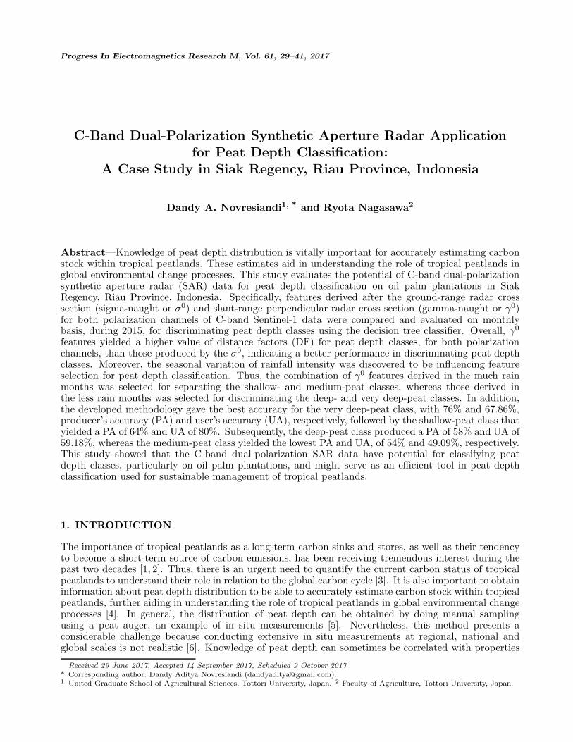
Progress In Electromagnetics Research M, Vol. 61, 29–41, 2017

C-Band Dual-Polarization Synthetic Aperture Radar Applicationfor Peat Depth Classification:

A Case Study in Siak Regency, Riau Province, Indonesia

Dandy A. Novresiandi1, * and Ryota Nagasawa2

Abstract—Knowledge of peat depth distribution is vitally important for accurately estimating carbonstock within tropical peatlands. These estimates aid in understanding the role of tropical peatlands inglobal environmental change processes. This study evaluates the potential of C-band dual-polarizationsynthetic aperture radar (SAR) data for peat depth classification on oil palm plantations in SiakRegency, Riau Province, Indonesia. Specifically, features derived after the ground-range radar crosssection (sigma-naught or σ0) and slant-range perpendicular radar cross section (gamma-naught or γ0)for both polarization channels of C-band Sentinel-1 data were compared and evaluated on monthlybasis, during 2015, for discriminating peat depth classes using the decision tree classifier. Overall, γ0

features yielded a higher value of distance factors (DF) for peat depth classes, for both polarizationchannels, than those produced by the σ0, indicating a better performance in discriminating peat depthclasses. Moreover, the seasonal variation of rainfall intensity was discovered to be influencing featureselection for peat depth classification. Thus, the combination of γ0 features derived in the much rainmonths was selected for separating the shallow- and medium-peat classes, whereas those derived inthe less rain months was selected for discriminating the deep- and very deep-peat classes. In addition,the developed methodology gave the best accuracy for the very deep-peat class, with 76% and 67.86%,producer’s accuracy (PA) and user’s accuracy (UA), respectively, followed by the shallow-peat class thatyielded a PA of 64% and UA of 80%. Subsequently, the deep-peat class produced a PA of 58% and UA of59.18%, whereas the medium-peat class yielded the lowest PA and UA, of 54% and 49.09%, respectively.This study showed that the C-band dual-polarization SAR data have potential for classifying peatdepth classes, particularly on oil palm plantations, and might serve as an efficient tool in peat depthclassification used for sustainable management of tropical peatlands.

1. INTRODUCTION

The importance of tropical peatlands as a long-term carbon sinks and stores, as well as their tendencyto become a short-term source of carbon emissions, has been receiving tremendous interest during thepast two decades [1, 2]. Thus, there is an urgent need to quantify the current carbon status of tropicalpeatlands to understand their role in relation to the global carbon cycle [3]. It is also important to obtaininformation about peat depth distribution to be able to accurately estimate carbon stock within tropicalpeatlands, further aiding in understanding the role of tropical peatlands in global environmental changeprocesses [4]. In general, the distribution of peat depth can be obtained by doing manual samplingusing a peat auger, an example of in situ measurements [5]. Nevertheless, this method presents aconsiderable challenge because conducting extensive in situ measurements at regional, national andglobal scales is not realistic [6]. Knowledge of peat depth can sometimes be correlated with properties

Received 29 June 2017, Accepted 14 September 2017, Scheduled 9 October 2017* Corresponding author: Dandy Aditya Novresiandi ([email protected]).1 United Graduate School of Agricultural Sciences, Tottori University, Japan. 2 Faculty of Agriculture, Tottori University, Japan.

30 Novresiandi and Nagasawa

that are discernible by using a remote sensing (RS) application [7]. However, little is known regardingthe performance of RS applications for peat depth distribution classification, especially in the tropics.

RS applications can serve as advantageous tools for tropical peatlands monitoring activities,such as peat depth classification, due to periodic monitoring at various spatial and temporal scales,particularly when combined with field measurement data [4]. Furthermore, the recent development ofsynthetic aperture radar (SAR)-based RS satellites has introduced a new prospect that allows continuousmonitoring and cloud-free observations in humid tropical regions [8]. Recently, the use of SAR-basedRS applications for peatlands monitoring activities has been increasing rapidly, along with the growingavailability of SAR data sets. A previous study evaluated the potential of X-band dual-polarizationSAR data and fusion images with optical data to characterize different peat depths categories in CentralKalimantan, Indonesia [9]. Another report demonstrated the use of L-band Phased Array type L-bandSAR (PALSAR) for wide-area mapping of tropical forest and land cover, including several categoriesfor tropical peatlands on Borneo Island [10]. Other reports have evaluated the performance of L-bandPALSAR for peatlands detection and delineation in the boreal regions [11, 12]. A previous report alsoapplied the L-band PALSAR to examine a radar scattering mechanism on tropical peatlands in CentralKalimantan, Indonesia [13]. Another study examined the combination of L-band PALSAR data, opticaldata and digital elevation model (DEM)-derived data for mapping the extent of tropical peatlands inCuvette Centrale, Congo Basin [14]. Despite all the previous research, detailed information is lackingon the potential C-band dual-polarization SAR data have for classifying peat depth distribution withinthe tropical peatlands.

The C-band Sentinel-1 data provided by the European Space Agency (ESA) are of interest becausethey are freely available and have global coverage. The Sentinel-1 mission encompasses a constellationof two polar-orbiting satellites (Sentinel-1A and Sentinel-1B). This data collection method operates ata center frequency of 5.405 GHz and includes two polarization channels — vertical transmit-horizontalreceive (VH) and vertical transmit-vertical receive (VV) — with a very short repeat cycle (12 dayswith one satellite and 6 days with two) and rapid product delivery. These characteristics make C-bandSentinel-1 data particularly promising for use in tropical peatlands monitoring activity, particularly forclassifying peat depth distribution. Therefore, in this study, the potential of C-band Sentinel-1 data wasevaluated for peat depth classification on oil palm plantations in Siak Regency, Riau Province, Indonesia.Particularly, features derived after the ground-range radar cross section (sigma-naught or σ0) and slant-range perpendicular radar cross section (gamma-naught or γ0) for both polarization channels of C-bandSentinel-1 data were compared and evaluated, monthly during 2015, for discriminating peat depthclasses using the decision tree (DT) classifier. In addition, the seasonal variation of peat depth classes,from the viewpoint of C-band dual-polarization SAR data, was analyzed for better understanding of therelationship between peat depth classification and seasonal effects. The results and findings of this studycould aid in increasing the foundation of knowledge regarding peat depth classification, involving the useof C-band dual-polarization SAR data, to improve the sustainable management of tropical peatlands.

2. MATERIALS

2.1. Study Area

In Indonesia, there are 14.91 million ha of tropical peatlands that distributed along the low altitudesin the coastal and sub-coastal areas of Sumatra (6.44 million ha, 43%), Kalimantan (4.78 million ha,32%) and Papua (3.69 million ha, 25%) [15]. Riau Province in Sumatra dominates the provincial levelof tropical peatlands distribution, consisting of around 3.86 million ha (26%). This study considersthe area of Siak Regency, a rapidly developing region in the central part of Riau Province, where thetropical peatlands have been intensively converted into mostly oil palm and timber plantations over thelast two decades [16, 17]. In general, this area has a flat topography and low altitude ranging from 2 to10 m above sea level. The average temperature of this area is around 26.2◦C per year, with an annualrainfall that varies from 2200 to 2600 mm per year. However, in 2015, this area was affected by a verystrong El Nino, leading to rainfall anomalies and a more severe dry season [18].

Four study areas, 1× 1 km in size, were selected to represent the condition of tropical peatlands inSiak Regency, Riau Province, Indonesia (Fig. 1). These study areas are situated in large-scale oil palmplantations with similar types of growing stages. Furthermore, to represent peat depth categories, each

Progress In Electromagnetics Research M, Vol. 61, 2017 31

Figure 1. Map of Indonesia showing the location of the study areas in Siak Regency, Riau Province,Indonesia.

study area is located on distinct types of peat depth classes as categorized by the Indonesian Agency forAgricultural Research and Development (IAARD) [15]. Thus, study area 1 is situated in a shallow-peatclass (0.5 to 1 m of peat depth), study area 2 is situated in a medium-peat class (1 to 2 m of peat depth),study area 3 is situated in a deep-peat class (2 to 4 m of peat depth), and study area 4 is situated in avery deep-peat class (more than 4 m of peat depth).

2.2. Data

In this study, there were 12 scenes of C-band Sentinel-1 data, acquired between January and December2015, served as 12-months observations. Thus, each scene, with a specific acquisition date, was used torepresent a monthly observation to provide monthly analyses. These scenes were used as the primarydata. The C-band Sentinel-1 data were collected using the settings of level-1 Ground Range Detected(GRD) and the acquisition mode of Interferometric Wide (IW) swath [19]. Moreover, Tropical RainfallMeasuring Mission (TRMM) 3B43 version 7 data were used to calculate the amount of monthly rainfallin the study areas [20]. Landsat 8 Operational Land Imager (OLI) data and high-resolution satelliteimages on Google Earth were used to obtain basic information of the study areas by means of visualinterpretation and to select training and testing points for DT classification. A total of 600 points(150 points for each study area) were derived for training the algorithm (400 points) and testing theaccuracy of the classification results (200 points). Each point was located within a 100 × 100 m mesh,with manual adjustments made to avoid points situated on plantation roads. These points representedthe detected pixels in the C-band dual-polarization SAR imagery. In addition, an existing peat depthand distribution map, provided by the IAARD, was used as reference map. The list of data used foranalyses is shown in Table 1.

3. METHODOLOGY

3.1. Image Processing Steps

The C-band Sentinel-1 data were imported into the ESA Sentinel Application Platform (SNAP) softwarefor image processing [21]. First, the data were radiometrically calibrated and converted from digitalpixel values to radiometrically-calibrated backscatter by means of a calibration vector provided in thedata product. In this study, the C-band Sentinel-1 data were converted to ground-range radar crosssection (sigma-naught or σ0) and slant-range perpendicular radar cross section (gamma-naught or γ0)values, in decibel units (dB), for both channels of polarization prior to data analyses. Both σ0 and γ0

are measures used to express radar backscatter coefficients. However, σ0 is defined as the radar cross


Table 1. List of data used for analyses carried out in this study.

Data usage Source Acquisition date

Primary dataC-band Sentinel-1 data

(Sentinel-1A satellite, dual-polarization)

Jan. 3, 2015Feb. 19, 2015Mar. 4, 2015Apr. 21, 2015May 15, 2015Jun. 8, 2015Jul. 26, 2015Aug. 18, 2015Sep. 11, 2015Oct. 6, 2015Nov. 11, 2015Dec. 29, 2015

Secondary data

TRMM 3B43 version 7(Monthly 0.25 × 0.25 degree,

mm/hour of rainfall rate)

Monthly data betweenJanuary and December 2015

Landsat 8 OLIJul. 10, 2015Jul. 26, 2015Aug. 2, 2015

High-resolution satellite images accessedon Google Earth

Jul. 25, 2014Jul. 5, 2015

Aug. 26, 2016

section per unit area in the ground-range, whereas γ0 is defined as radar cross section per unit area ofthe incident wavefront (perpendicular to the slant-range), to minimize the incidence angle dependencyof the radar backscatter for a distributed target [22, 23].

Furthermore, the data were terrain corrected using SRTM DEM 3 arc-seconds [24] and geocoded tothe Universal Transverse Mercator (UTM) zone 48-north map projection with pixel spacing of 10×10 m.Speckle noise was reduced by applying a 7×7 window size Lee filter [25]. In addition, to provide rainfallinformation for the study areas, the precipitation layers of TRMM 3B43 version 7 data acquired betweenJanuary and December 2015 were extracted. Rainfall rate conversions from mm/hour to mm/monthwere calculated. The data were then subset into the boundaries of the study areas so that monthlyrainfall information could be generated for the analyses carried out in this study.

3.2. Feature Description

In this study, the σ0 and γ0 images, for both polarization channels, derived using the C-band Sentinel-1data, were considered as features. To allow for monthly analysis, each σ0 or γ0 image for a particularpolarization channel on a specific acquisition date was considered as one feature (e.g., a σ0 image forthe VH polarization channel acquired on January 3, 2015 was considered as one feature and coded assVH01; a γ0 image for the VV polarization channel acquired on November 11, 2015 was considered asone feature and coded as gVV11). Thus, a total of 48 features were derived, using the C-band Sentinel-1data, for the analyses carried out in this study. The list of features used for analyses is shown in Table 2.


Table 2. List of features used for analyses, derived using sigma naught (σ0) and gamma naught (γ0)images, for both polarization channels.

Polarization channel Acquisition date Sigma-naught code name Gamma-naught code name

VH

Jan. 3, 2015 sVH01 gVH01Feb. 19, 2015 sVH02 gVH02Mar. 4, 2015 sVH03 gVH03Apr. 21, 2015 sVH04 gVH04May 15, 2015 sVH05 gVH05Jun. 8, 2015 sVH06 gVH06Jul. 26, 2015 sVH07 gVH07Aug. 18, 2015 sVH08 gVH08Sep. 11, 2015 sVH09 gVH09Oct. 6, 2015 sVH10 gVH10Nov. 11, 2015 sVH11 gVH11Dec. 29, 2015 sVH12 gVH12

VV

Jan. 3, 2015 sVV01 gVV01Feb. 19, 2015 sVV02 gVV02Mar. 4, 2015 sVV03 gVV03Apr. 21, 2015 sVV04 gVV04May 15, 2015 sVV05 gVV05Jun. 8, 2015 sVV06 gVV06Jul. 26, 2015 sVV07 gVV07Aug. 18, 2015 sVV08 gVV08Sep. 11, 2015 sVV09 gVV09Oct. 6, 2015 sVV10 gVV10Nov. 11, 2015 sVV11 gVV11Dec. 29, 2015 sVV12 gVV12

3.3. Decision Tree (DT) Classification

To classify the peat depth classes using C-band Sentinel-1 data, DT classifier was used due to itsability to handle complex relations among class properties, its computational efficiency and conceptualsimplicity [26]. DT is a classification procedure that recursively separates a set of data into smallersubcategories based on a set of rules determined at each branch in the tree. It requires no assumptionsregarding the distributions of input data, making it suitable for classifying SAR data [27]. Furthermore,DT algorithm diagrams are explicit and easy to understand, particularly when evaluating featurecontributions and relations in a classification procedure [28].

3.4. Distance Factor (DF) Extraction

In this study, the distance factor (DF) was generated to assess the effectiveness of a feature for separatingclasses, particularly on DT classification. The DF measures the distance between the different class meanvalues compared to the standard deviations. Thus, if a DF is large, classes are said to be well-separated,according to the concept of feature separation [29]. The DF is defined as:

DF ij =|xi − xj|σi + σj

, (1)


where x represents the mean values and σ the standard deviations. The performance of the separationbetween classes i and j is represented by the value DFij. A higher DFij means that a feature hasbetter performance separating the associate class pairs [30]. Thus, in this study, features that yieldedthe highest DF value on each class pair for each polarization channel were analyzed and applied to theDT algorithm.

In the present study, to apply the concept of feature separation on the DT algorithm, threecombinations of class pairs were specified (i.e., (A) “shallow-peat” plus “medium-peat” and “deeppeat” plus “very-deep peat”, (B) “shallow-peat” and “medium-peat,” and (C) “deep-peat” and “very-deep peat.” The class pairs were then applied to the DT algorithm to identify each peat depth class.In addition, the selected features for each class pair were analyzed to understand the effect seasonalvariation has upon peat depth classifications. Hence, the monthly rainfall information, derived fromthe TRMM 3B43 version 7 data, was used for seasonal analysis purposes.

3.5. Accuracy Assessment

An accuracy assessment was performed for the classification results using a confusion matrix generatedby testing points [31]. Thus, accuracy indicators were derived to evaluate the quality of classificationresults (i.e., Producer’s Accuracy (PA), User’s Accuracy (UA), Overall Accuracy (OA) and the Kappacoefficient (K)). The PA and UA represent the measures of omission and commission error for eachclass, respectively. The OA was computed by creating a ratio of the total number of correct pixels tothe total number of pixels in the confusion matrix, which correspond to the correctly classified areas ofthe classified image. Last, the K describes the degree of matching between the reference data set andthe classification.

4. RESULTS AND DISCUSSION

4.1. Comparison of σ0 and γ0 Features

Table 3 shows the DF values for class pair (A), derived using σ0 and γ0 features, for both polarizationchannels. The values in bold indicate the highest DF values in each category. Generally, the DF valuesof class pair (A) were varied, depending on the feature used to derive them. The sVH06 (σ0

VH in June)and sVV06 (σ0

VV in June) features yielded the highest DF values for those derived using σ0VH and σ0

VV

features, respectively. On the other hand, the gVH06 (γ0VH in June) and gVV06 (γ0

VV in June) featuresproduced the highest DF values for those derived using γ0

VH and γ0VV features, respectively.

Thus, by comparing the highest DF values of class pair (A), derived using σ0 and γ0 features, forboth polarization channels, it was found that γ0 features yielded much higher DF values for class pair(A), for both polarization channels, than those produced by σ0 features. By applying γ0 features, thehighest DF values of class pair (A) increased as much as 11.5% and 13.3% for VH and VV polarizations,respectively. Hence, in this study, γ0 features were used for developing a methodology for classifyingpeat depth due to the features having better performance in discriminating peat depth classes.

4.2. Selected Features for the Classification

Table 4 shows the DF values for all class pairs, derived by γ0 features, for both polarization channels.The values in bold indicate the highest DF values in each category. The highest values were selectedto be analyzed and applied to the DT algorithm. In general, the DF values for all class pairs varied,depending on the features used to derive them. For class pair (A), as mentioned before, the gVH06 (γ0

VH

in June) and gVV06 (γ0VV in June) features yielded the highest DF values for VH and VV polarization,

respectively. On the other hand, for class pair (B), the gVH03 (γ0VH in March) and gVV04 (γ0

VV inApril) features produced the highest DF values for VH and VV polarization, respectively. Furthermore,for class pair (C), the gVH06 (γ0

VH in June) and gVV09 (γ0VV in September) features generated the

highest DF values for VH and VV polarization, respectively. These features were selected and appliedto the DT algorithm for classifying peat depth classes.


Table 3. The distance factor (DF) values for class pair (A), derived using sigma naught (σ0) andgamma naught (γ0) features, for both polarization channels.

Feature Class pair (A)Polarization channel Acquisition date Sigma naught Gamma naught

VH

Jan. 3, 2015 0.18 0.12Feb. 19, 2015 0.51 0.44Mar. 4, 2015 0.44 0.50Apr. 21, 2015 0.05 0.01May 15, 2015 0.10 0.04Jun. 8, 2015 0.52 0.58Jul. 26, 2015 0.41 0.35Aug. 18, 2015 0.15 0.08Sep. 11, 2015 0.22 0.15Oct. 6, 2015 0.11 0.17Nov. 11, 2015 0.06 0.13Dec. 29, 2015 0.04 0.09

VV

Jan. 3, 2015 0.06 0.12Feb. 19, 2015 0.40 0.33Mar. 4, 2015 0.41 0.46Apr. 21, 2015 0.19 0.25May 15, 2015 0.03 0.02Jun. 8, 2015 0.45 0.51Jul. 26, 2015 0.04 0.11Aug. 18, 2015 0.31 0.24Sep. 11, 2015 0.32 0.25Oct. 6, 2015 0.32 0.37Nov. 11, 2015 0.09 0.15Dec. 29, 2015 0.00 0.07

In addition, by examining the highest DF values for all class pairs, derived by γ0 features, forboth polarization channels, it was found that γ0

VH features produced much higher DF values thanthose generated by γ0

VV features, indicating that the γ0VH features yielded a better performance in

discriminating peat depth classes. However, in this study, all γ0 features that obtained the highest DFvalues for both polarization channels were applied to the DT algorithm. Moreover, among all the classpairs, class pair (B) yielded the highest DF values for both polarization channels, indicating that themean and standard deviation values of the shallow- and medium-peat classes represented in class pair(B) overlapped less, obtaining a higher DF values than those derived in the other class pairs.

4.3. Seasonal Variation of the Selected Features

To understand the effect of seasonal variation on the selected features for peat depth classification,monthly rainfall information derived from the TRMM 3B43 version 7 data was used for seasonalanalysis purposes. In 2015, a year with a very strong El Nino, the annual rainfall was as low as1992 mm, with an average monthly rainfall of 166 mm. For the seasonal analyses carried out in thisstudy, months with below average monthly rainfall were said to be “less rain” months, whereas those


Table 4. The distance factor (DF) values for all class pairs, derived using gamma-naught (γ0) features,for both polarization channels.

Feature Class pairPolarization channel Code name (A) (B) (C)

VH

gVH01 0.12 0.23 0.18gVH02 0.44 0.22 0.31gVH03 0.50 0.75 0.08gVH04 0.01 0.28 0.59gVH05 0.04 0.60 0.15gVH06 0.58 0.05 0.60gVH07 0.35 0.34 0.43gVH08 0.08 0.48 0.20gVH09 0.15 0.40 0.18gVH10 0.17 0.27 0.07gVH11 0.13 0.07 0.41gVH12 0.09 0.13 0.57

VV

gVV01 0.12 0.34 0.28gVV02 0.33 0.48 0.44gVV03 0.46 0.62 0.55gVV04 0.25 0.71 0.04gVV05 0.02 0.65 0.42gVV06 0.51 0.38 0.05gVV07 0.11 0.38 0.29gVV08 0.24 0.50 0.51gVV09 0.25 0.48 0.56gVV10 0.37 0.30 0.48gVV11 0.15 0.36 0.12gVV12 0.07 0.28 0.07

with above average rainfall were said to be “much rain” months. Hence, the less rain months areJanuary (149 mm/month), February (141 mm/month), May (146 mm/month), June (119 mm/month),July (46 mm/month), September (52 mm/month), and October (78 mm/month), whereas the muchrain months are March (269 mm/month), August (222 mm/month), November (330 mm/month), andDecember (254 mm/month).

For class pair (A) (derived by both σ0 and γ0), features acquired in June yielded the highest DFvalue for both polarization channels. Thus, for the initial separation of peat depth classes representedin class pair (A), features derived in the less rain months were prominent. In contrast, for class pair(B), features acquired in March and April produced the highest DF value for VH and VV polarization,respectively. Hence, for more detailed separation of peat depth classes, (i.e., separating the shallow-and medium-peat classes) features derived in the much rain months were suitable. On the other hand,for class pair (C), features acquired in June and September generated the highest DF value for VHand VV polarization, respectively. Therefore, features derived in the less rain months were suitablefor separating the deep- and very deep-peat classes. In this study, it was discovered that seasonalvariation influenced feature selection for peat depth classification, particularly when analyzing C-banddual-polarization SAR data.


4.4. Results of the Classification

The selected features for peat depth classification were the gVH06 (γ0VH in June) and gVV06 (γ0

VV inJune), for separating classes in the class pair (A). Subsequently, the gVH03 (γ0

VH in March) and gVV04(γ0

VV in April) were selected for discriminating peat depth classes in the class pair (B). Afterwards, thegVH06 (γ0

VH in June) and gVV09 (γ0VV in September) were selected for separating peat depth classes in

the class pair (C). Thus, a total of three classification rules, separating three class pairs, were generatedusing training points based on the selected features for peat depth classification. The classification ruleswere developed using mean and standard deviation values of peat depth classes for each selected feature.These rules are listed as follows:

(i) Rule 1 for separating classes in the class pair (A).If gVH06 (γ0

VH in June) ≥ (−13.20) dB and gVV06 (γ0VV in June) ≥ (−4.97) dB, Then Class pair

(B).(ii) Rule 2 for separating peat depth classes in the class pair (B).

If gVH03 (γ0VH in March) ≥ (−13.55) dB and gVV04 (γ0

VV in April) ≥ (−5.31) dB, Then Shallowpeat.

(iii) Rule 3 for separating peat depth classes in the class pair (C).If gVH06 (γ0

VH in June) ≥ (−12.71) dB and gVV09 (γ0VV in September) ≤ (−4.88) dB, Then Deep

peat.

These classification rules were then applied to the DT algorithm to obtain classification results. Theclassification rules and DT algorithm diagram developed in this study are shown in Fig. 2. Afterwards,as shown in Fig. 3, results of the peat depth classification of all study areas were successfully generatedby means of DT classification. These results presented four peat depth classes (i.e., shallow peat (0.5to 1 m of peat depth), medium peat (1 to 2m of peat depth), deep peat (2 to 4m of peat depth), andvery-deep peat (more than 4 m of peat depth).

Figure 2. The classification rules and the decision tree (DT) algorithm diagram developed in thisstudy.

Table 5. The pixel percentage of each peat depth class calculated in each study area. The values inbold indicate the highest pixel percentage of peat depth classes produced on each study area.

Study areaPixel percentage (%)

Shallow peat Medium peat Deep peat Very-deep peat1 56.37 18.45 14.81 10.372 11.74 43.17 31.81 13.283 2.82 18.42 48.42 30.344 1.84 13.44 13.96 70.76


(a)

(c)

(b)

(d)

Figure 3. The result of the peat depth classification of (a) study area 1, (b) study area 2, (c) studyarea 3, and (d) study area 4.

In addition, Table 5 shows the pixel percentage of each peat depth class calculated in each studyarea. Thus, by comparing the actual peat depth condition of each study area and the pixel percentage ofpeat depth classes computed on the associated study area, it was found that the developed methodologywas always successful in matching the actual peat depth condition with the highest pixel percentageof peat depth classes produced. Hence, in study area 1, an area situated in shallow peat, the highestpixel percentage (56.37%) was yielded for the shallow-peat class. Subsequently, in study area 2, anarea situated in medium peat, the highest pixel percentage (43.17%) was produced for the medium-peatclass. Next, in study area 3, an area situated in deep peat, the highest pixel percentage (48.42%) wasgenerated for the deep-peat class. Last, in study area 4, an area situated in very deep peat, the highestpixel percentage (70.76%) was yielded for the very deep-peat class. Furthermore, best performanceof the developed methodology was found in very deep-peat areas, represented in study area 4, as themethodology generated much higher pixel percentages of peat depth classes that matched with actualpeat depth conditions, compared to those derived in other study areas.


4.5. Accuracies of the Classification

Table 6 shows the confusion matrix and accuracy indicators for peat depth classifications by means ofDT classification. The accuracy assessment was conducted by using the testing points situated in thestudy areas, evaluating the performance of the developed peat depth classifications. Thus, the verydeep-peat class obtained the best accuracy, with 76% and 67.86%, PA and UA, respectively, followedby the shallow-peat class that yielded a PA of 64% and UA of 80%. Subsequently, the deep-peat classproduced a PA of 58% and UA of 59.18%, whereas the medium-peat class yielded the lowest PA andUA, of 54% and 49.09%, respectively. This result showed that the C-band dual-polarization SAR datahave potential for classifying peat depth classes, particularly on oil palm plantations, due to its abilityto produce the best accuracy for the very deep-peat class that is difficult to be distinguished amongpeat depth classes [4]. In addition, the developed methodology gave accuracies of 63% and 0.51, forOA and K, respectively. This value of K was considered as a moderate agreement of a classificationresult [32]. Furthermore, the accuracy assessment result agreed with the analysis result for the pixelpercentage of peat depth classes generated on each study area as presented in Section 4.4, whereby thedeveloped methodology consistently gave the best performance for the very deep-peat areas.

Table 6. The confusion matrix and accuracy indicators for peat depth classifications using the decisiontree (DT) classification.

ReferenceTotal

Producer’s

Accuracy

(%)

User’s

Accuracy

(%)Class

Shallow

peat

Medium

peat

Deep

peat

Very-deep

peat

Shallow

peat32 7 1 0 40 64.00 80.00

Medium

peat11 27 11 6 55 54.00 49.09

Deep

peat3 11 29 6 49 58.00 59.18

Very-deep

peat4 5 9 38 56 76.00 67.86

Total 50 50 50 50 200

Overall

Accuracy (%)63.00

Kappa

coefficient0.51

5. CONCLUSION

This study evaluated the potential of C-band Sentinel-1 data for peat depth classification on oil palmplantations, by using a SAR-based RS application, in response to the emerging tropical peatlandsmonitoring activities. Several findings were obtained relating to the development of peat depthclassification using C-band dual-polarization SAR data. First, the present study showed that the γ0

features yielded better performance in discriminating peat depth classes. By comparing the highest DFvalues of class pair (A), derived using σ0 and γ0 features, for both polarization channels, it was foundthat γ0 features yielded much higher DF values for class pair (A), for both polarization channels, thanthose produced by σ0 features. Thus, by applying γ0 features, the DF values of class pair (A) increasedas much as 11.5% and 13.3% for VH and VV polarizations, respectively. Second, it was discovered thatseasonal variation was influencing feature selection for peat depth classification. Both γ0

VH and γ0VV, in

the much rain months, were selected for separating the shallow- and medium-peat classes in class pair(B), whereas both γ0

VH and γ0VV, in the less rain months, were selected for discriminating the deep- and


very deep-peat classes in class pair (C). Third, the developed methodology gave the best accuracy forthe very deep-peat class, with 76% and 67.86%, producer’s accuracy (PA) and user’s accuracy (UA),respectively, followed by the shallow-peat class that yielded a PA of 64% and UA of 80%. Subsequently,the deep-peat class produced a PA of 58% and UA of 59.18%, whereas the medium-peat class yieldedthe lowest PA and UA, of 54% and 49.09%, respectively. Moreover, it was discovered that the developedmethodology was always successful in matching the actual peat depth condition with the highest pixelpercentage of peat depth classes generated. Furthermore, accuracy assessment results agreed with theanalysis results for the pixel percentage of peat depth classes produced in each study area, whereby thedeveloped methodology was consistent in providing the best performance for very deep-peat areas. Theresults and findings in this study show that the C-band Sentinel-1 data are suitable for classifying peatdepth classes, particularly on oil palm plantations, and might serve as an efficient tool in peat depthclassification used for sustainable management of tropical peatlands.

REFERENCES

1. Osaki, M., D. Nursyamsi, M. Noor, Wahyunto, and H. Segah, “Peatland in Indonesia,” TropicalPeatland Ecosystems, M. Osaki and N. Tsuji (eds)., 49–58, Springer, Tokyo, Japan, 2016.

2. Miettinen, J., A. Hooijer, R. Vernimmen, S. C. Liew, and S. E. Page, “From carbon sink to carbonsource: extensive peat oxidation in insular Southeast Asia since 1990,” Environmental ResearchLetters, Vol. 12, No. 024014, 1–10, 2017.

3. Hirano, T., S. Sundari, and H. Yamada, “CO2 balance of tropical peat ecosystems,” TropicalPeatland Ecosystems, M. Osaki and N. Tsuji (eds.), 329–338, Springer, Tokyo, Japan, 2016.

4. Shimada, S., H. Takahashi, and M. Osaki, “Carbon stock estimate,” Tropical Peatland Ecosystems,M. Osaki and N. Tsuji (eds.), 455–467, Springer, Tokyo, Japan, 2016.

5. Agus, F., K. Hairiah, and A. Mulyani, Measuring Carbon Stock in Peat Soils: Practical Guidelines,World Agroforestry Centre (ICRAF) Southeast Asia Regional Program and Indonesian Centre forAgricultural Land Resources Research and Development, Bogor, Indonesia, 2011.

6. Jaenicke, J., J. O. Rieley, C. Mott, P. Kimman, and F. Siegert, “Determination of the amount ofcarbon stored in Indonesian peatlands,” Geoderma, Vol. 147, 151–158, 2008.

7. Lawson, I. T., T. J. Kelly, P. Aplin, A. Boom, G. Dargie, F. C. H. Draper, P. N. Z. B. P. Hassan,J. Hoyos-Santillan, J. Kaduk, D. Large, W. Murphy, S. E. Page, K. H. Roucoux, S. Sjogersten,K. Tansey, M. Waldram, B. M. M. Wedeux, and J. Wheeler, “Improving estimates of tropicalpeatland area, carbon storage, and greenhouse gas fluxes,” Wetlands Ecology Management, Vol. 23,327–346, 2015.

8. Kuntz, S., “Potential of spaceborne SAR for monitoring the tropical environments,” TropicalEcology, Vol. 51, No. 1, 3–10, 2010.

9. Wijaya, A., P. R. Marpu, and R. Gloaguen, “Discrimination of peatlands in tropical swamp forestsusing dual-polarimetric SAR and Landsat ETM data,” International Journal of Image Data Fusion,Vol. 1, No. 3, 257–270, 2010.

10. Hoekman, D. H., M. A. M. Vissers, and N. Wielaard, “PALSAR wide-area mapping of borneo:methodology and map validation,” IEEE Journal of Selected Topics in Applied Earth Observationsand Remote Sensing, Vol. 3, No. 4, 605–617, 2010.

11. Antropov, O., Y. Rauste, J. Praks, M. Hallikainen, and T. Hame, “Peatland delineation underforest canopy with polsar data using model based decomposition technique,” Proceeding IEEEInternational Geoscience and Remote Sensing Symposium, 4918–4921, 2012.

12. Antropov, O., Y. Rauste, H. Astola, J. Praks, T. Hame, and M. T. Hallikainen, “Land cover andsoil type mapping from spaceborne PolSAR data at L-band with probabilistic neural network,”IEEE Transactions on Geoscience and Remote Sensing, Vol. 52, No. 9, 5256–5270, 2014.

13. Watanabe, M., K. Kushida, and C. Yonezawa, “PALSAR full-polarimetric observation forpeatland,” Asian Journal of Geoinformatics, Vol. 11, No. 3, 2011.


14. Dargie, G. C, S. L. Lewis, I. T. Lawson, E. T. A. Mitchard, S. E. Page, Y. E. Bocko, and S. A. Ifo,“Age, extent and carbon storage of the central Congo Basin peatland complex,” Nature, Vol. 542,No. 2, 86–90, 2017.

15. Ritung, S., Wahyunto, and K. Nugroho, “Karakteristik dan sebaran lahan gambut di Sumatera,Kalimantan dan Papua,” Pengelolaan Lahan Gambut Berkelanjutan, E. Husen, M. Anda, M. Noor,H. S. Mamat, Maswar, A. Fahmi, and Y. Sulaiman (eds.), BBSDLP, Bogor, Indonesia, 2012.

16. Sabiham, S. and S. Kartawisastra, “Peatland management for oil palm development in indonesia,”Indonesian Journal of Land Resources, Vol. 6, No. 2, 55–66, 2012.

17. Irawan, S. and L. Tacconi, Intergovernmental Fiscal Transfer, Forest Conservation and ClimateChange, Edward Elgar, Cheltenham, UK, 2016.

18. Englhart, S., M. Staengel, and F. Siegert, “Estimation of fire affected areas and carbon emissionson the basis of Sentinel-1,” Proceedings of the 15th International Peat Congress 2016: PosterPresentations, 370–374, Kuching, Sarawak, Malaysia, 2016.

19. Dimov, D., J. Kuhn, and C. Conrad, “Assessment of cropping system diversity in the FerganaValley through image fusion of Landsat 8 and Sentinel-1,” ISPRS Annals of the Photogrammetry,Remote Sensing and Spatial Information Sciences, Vol. III-7, 173–180, 2016.

20. Huffman, G. J., R. F. Adler, D. T. Bolvin, and E. J. Nelkin, “The TRMM Multi-satellitePrecipitation Analysis (TMPA),” Satellite Rainfall Applications for Surface Hydrology, F. Hossainand M. Gebremichael (eds.), 3–22, Springer Verlag, 2010.

21. Luis, V., J. Lu, M. Foumelis, and M. Engdahl, “ESA’s multi-mission Sentinel-1 Toolbox,”Proceedings of the 19th EGU General Assembly, 19398, Vienna, Austria, 2017.

22. Shimada, M., “Ortho-rectification and slope correction of SAR data using DEM and its accuracyevaluation,” IEEE Journal of Selected Topics in Applied Earth Observations and Remote Sensing,Vol. 3, No. 3, 657–671, 2010.

23. El-Darymli, K., P. McGuire, E. Gill, D. Power, and C. Moloney, “Understanding the significance ofradiometric calibration for synthetic aperture radar imagery,” Canadian Conference on Electricaland Computer Engineering, Toronto, Canada, 2014.

24. Farr, T. G., et al., “The shuttle radar topography mission,” Reviews of Geophysics, Vol. 45, No. 2,RG2004, 2007.

25. Lee, J. and E. Pottier, Polarimetric SAR Radar Imaging: From Basic to Applications, CRC Press,Taylor & Francis Group, 2009.

26. Friedl, M. A. and C. E. Brodley, “Decision tree classification of land cover from remotely senseddata,” Remote Sensing of Environment, Vol. 61, 399–409, 1997.

27. Simard, M., S. S. Saatchi, and G. D. Grandi, “The use of decision tree and multiscale texturefor classification of JERS-1 SAR data over tropical forest,” IEEE Transactions on Geoscience andRemote Sensing, Vol. 38, No. 5, 2310–2321, 2000.

28. Simard, M., G. D. Grandi, S. Saatchi, and P. Mayaux, “Mapping tropical coastal vegetation usingJERS-1 and ERS-1 radar data with a decision tree classifier,” International Journal of RemoteSensing, Vol. 23, No. 7, 1461–1474, 2002.

29. Cumming, I. G. and J. J. Van Zyl, “Feature utility in polarimetric radar image classification,”Proceeding IEEE International Geoscience and Remote Sensing Symposium, 1841–1846, 1989.

30. Chen, J., H. Lin, and Z. Pei, “Application of ENVISAT ASAR data in mapping rice crop growthin southern China,” IEEE Geoscience and Remote Sensing Letters, Vol. 4, No. 3, 431–435, 2007.

31. Congalton, R. G., “A review of accessing the accuracy of classifications of remotely sensed data,”Remote Sensing Environment, Vol. 37, 35–46, 1991.

32. Viera, J. A. and J. M. Garrett, “Understanding interobserver agreement: The kappa statistic,”Family Medicine, Vol. 37, No. 5, 360–363, 2005.

Documents

C-Band Dual-Polarization Synthetic Aperture Radar ...jpier.org/PIERM/pierm61/03.17062903.pdf · C-Band Dual-Polarization Synthetic Aperture Radar Application ... A Case Study in Siak