C #38 1 N 30 N 2013 - European Space Agency · CRYO SAT CYCLIC REPORT CYCLE #38 1ST NOVEMBER 2013 – 30 TH NOVEMBER 2013 Prepared by/ préparé par CryoSat IDEAS Team Reference

CRYOSAT

CYCLIC REPORT

CYCLE #38

1ST NOVEMBER 2013 – 30TH NOVEMBER 2013

Prepared by/ préparé par CryoSat IDEAS Team Reference/ réference Issue/ édition 1 Revision/ révision 0

Date of issue/ date d’édition 13 February 2014 Document type/ type de document Technical Note

Issue 1 Revision 0 – 13 February 2014 page ii of iv

A P P R O V A L

Title titre

CryoSat Cyclic Report – Cycle 38 Issue issue

1 Revision revision

0

Author auteur

IDEAS CryoSat QC Team Date date

13 February 2014

C H A N G E L O G

Reason for change raison du changement

Issue issue

Revision revision

Date date

C H A N G E R E C O R D

ISSUE: 1 REVISION: 0

Reason for change raison du changement

Page(s) page(s)

Paragraph(s) paragraph(s)

Issue 1 Revision 0 – 13 February 2014 page iii of iv

T A B L E O F C O N T E N T S

1 INTRODUCTION ..................................................................................................................................... 1

1.1 Acronyms and Abbreviations ........................................................................................................ 2

1.2 Reference Documents .................................................................................................................. 2

2 CYCLE OVERVIEW ................................................................................................................................ 3

3 SOFTWARE & AUX FILE VERSION CONFIGURATION ....................................................................... 4

3.1 IPF Software Version ................................................................................................................... 4

3.2 Processor Versions for IPF1 and IPF2 ......................................................................................... 4

3.3 Auxiliary Files ............................................................................................................................... 5

3.3.1 Static Auxiliary Files ................................................................................................................. 5

3.3.2 Dynamic Auxiliary Files............................................................................................................. 6

3.3.3 Changes of Auxiliary Files during the cycle............................................................................... 6

4 PDS STATUS ......................................................................................................................................... 7

4.1 SIRAL Instrument Unavailability ................................................................................................... 7

4.2 SIRAL Level 0 Data Availability .................................................................................................... 7

4.3 SIRAL Level 1B and Level 2 FDM Data Availability ...................................................................... 8

4.4 SIRAL Level 1B and Level 2 Offline Data Availability ................................................................... 9

5 SIRAL HEALTH MONITORING ............................................................................................................ 10

5.1 Loss of Track .............................................................................................................................. 10

5.2 Acquisition Analysis .................................................................................................................... 11

6 FDM DATA QUALITY CONTROL ........................................................................................................ 12

6.1 Product Format Checks .............................................................................................................. 12

6.2 Software Version Checks ........................................................................................................... 12

6.3 Forecast Auxiliary Data File Usage Checks ................................................................................ 12

6.4 External Forecast Auxiliary Corrections ...................................................................................... 13

6.4.1 Dry Tropospheric Correction ................................................................................................... 13

6.4.2 Wet Tropospheric Correction .................................................................................................. 14

6.4.3 Inverse Barometric Correction ................................................................................................ 15

6.4.4 Ionospheric Correction ........................................................................................................... 16

6.4.5 Sea State Bias Correction ...................................................................................................... 17

7 OFFLINE DATA QUALITY CONTROL ................................................................................................. 18

7.1 Product Format Checks .............................................................................................................. 18

7.2 Software Version Checks ........................................................................................................... 18

7.3 Auxiliary Data File Usage Checks .............................................................................................. 18

7.4 Product Parameters ................................................................................................................... 19

7.4.1 Monitoring of SIRAL Mode Changes....................................................................................... 19

7.4.2 Surface Type .......................................................................................................................... 21

7.4.3 Backscatter (Sigma0) ............................................................................................................. 22

7.4.4 Waveform Peakiness .............................................................................................................. 25

7.4.5 Freeboard ............................................................................................................................... 28

7.4.6 Snow Depth ............................................................................................................................ 28

7.4.7 Sea Ice Concentration ............................................................................................................ 29

7.4.8 Snow Density ......................................................................................................................... 30

7.4.9 Surface Height ........................................................................................................................ 30

7.5 Quality Flags .............................................................................................................................. 32

7.6 Crossover Analysis ..................................................................................................................... 33

7.6.1 CrossOver Statistics ............................................................................................................... 33

Issue 1 Revision 0 – 13 February 2014 page iv of iv

7.6.2 Elevation Maps ....................................................................................................................... 34

7.6.3 Backscatter (sigma0) Maps .................................................................................................... 36

7.7 External Auxiliary Corrections..................................................................................................... 38

7.7.1 Dry Tropospheric Correction ................................................................................................... 38

7.7.2 Wet Tropospheric Correction .................................................................................................. 39

7.7.3 Inverse Barometric correction ................................................................................................. 41

7.7.4 Dynamic Atmosphere correction ............................................................................................. 42

7.7.5 Ionospheric Correction ........................................................................................................... 44

8 ANOMALY REPORTS .......................................................................................................................... 46

9 README DOCUMENTS ON PERFORMANCE AND QUALITY ........................................................... 47

Issue 1 Revision 0 – 13 February 2014 page 1 of 47

1 INTRODUCTION CryoSat is an altimetry satellite built by the European Space Agency (ESA) and dedicated to polar observation. It embarked on a three-and-a-half-year mission to determine variations in the thickness of the Earth's continental ice sheets and marine ice cover, and to test the prediction of thinning Arctic ice due to climate change. CryoSat is designed to acquire continuously, switching automatically between its three measurement modes according to a Geographical Mode Mask:

- Synthetic Aperture Radar (SAR) is operated over sea-ice and over some ocean basins and coastal zones.

- SAR Interferometric (SARIn) mode is used over steeply sloping ice-sheet margins, small ice caps

and areas of mountain glaciers. It is also used over some major hydrological river basins and some ocean areas with important mesoscale variability.

- Low Resolution Mode (LRM) is operated over the areas of the continental ice sheets, over

oceans and over land not covered by other modes. This CryoSat Cyclic Report is distributed by IDEAS team to keep the CryoSat community informed of the overall mission performance and the status of the SIRAL instrument. The report is based on a 30-day reporting period, which has been defined by UCL/MSSL since the Transfer to Operations (TTO), as part of the routine QA monitoring activity. This 30-day cycle has been defined purely for the purpose of statistic reporting and does not correspond to an official 30-day sub cycle. The actual repeat cycle for CryoSat is 369 days, which consists of 5344 orbits. This document reports on both the Near Real Time (NRT) Fast Delivery Marine (FDM) mode data and Offline Science data. FDM data products are produced from LRM data only and are made available within three hours of measurement acquisition. Offline Science data products are processed with the DORIS Precise Orbits and as a result are generated with a delay of ~30 days after measurement acquisition. This document is available online at: http://earth.eo.esa.int/missions/cryosat/reports/cyclic/.


1.1 Acronyms and Abbreviations AR Anomaly Report CFI Customer Furnished Item CNES Centre National d'Études Spatiales CPOM Centre for Polar Observation Modelling DAC Dynamic Atmospheric Correction DEM Digital Elevation Model ECMWF European Centre for Medium-term Weather Forecasting ESA European Space Agency ESOC European Space Operation Centre FDM Fast Delivery Marine mode GDR Geophysical Data Record GIM Global Ionospheric Map GPS Global Positioning System IDEAS Instrument Data quality Evaluation and Analysis Service IPF Instrument Processing Facility L0/L1B/L2 Level 0/Level 1B/Level 2 LRM Low Resolution Mode LTA Long Term Archive MF Monitoring Facility MSSL Mullard Space Science Laboratory NRT Near Real Time OCM Orbit Control Manoeuvre PCONF Parameter Configuration File PDS Payload Data System QA Quality Assurance QCC Quality Control for CryoSat RMS Root Mean Square SSALTO Systeme au Sol d'Altimetrie et d'Orbitographie SSB Sea State Bias SAR Synthetic Aperture Radar mode SARIn SAR Interferometric mode SID SARIn Degraded SIRAL SAR Interferometric Radar Altimeter SPR Software Problem Report SW Software TTO Transfer to Operations UCL University College London WGS84 World Geodetic System of 1984

1.2 Reference Documents RD.1 CRYOSAT Ground Segment Instrument Processing Facility (IPF) L1B Products Format Specification, CS-RS-ACS-GS-5106, 4.9 RD.2 CRYOSAT Ground Segment IPF Level 2 (L2) Products Format Specification, CS-RS-ACS-GS-5123, 2.8 RD.3 Updated list of CryoSat IPF Anomalies. Latest version is available online at: http://earth.eo.esa.int/missions/cryosat/data_status/.


2 CYCLE OVERVIEW

Cyclic Number: 38

Cycle Start: 1st November 2013

Cycle End: 30th November 2013 The health of the SIRAL instrument and the quality of all Level 1B (L1B) and L2 data products was nominal throughout this cycle.


3 SOFTWARE & AUX FILE VERSION CONFIGURATION

3.1 IPF Software Version The versions of the IPF software installed within the Payload Data System (PDS) are listed below:

CryoSat IPF for Level 1 (IPF1): Version Vk2.0

CryoSat IPF for Level 2 (IPF2): Version Vk1.0

3.2 Processor Versions for IPF1 and IPF2 The current versions of each processor versions within IPF1 and IPF2 are listed below:

L1B Products Processor Version

L1B LRM SIR1LRM/4.1

L1B SAR SIR1SAR/4.1

L1B SARIN SARIN/4.1

L1B FDM SIR1FDM/2.4

CAL1 LRM SIR1LRC1/4.0

CAL1 SAR SIR1SAC1/4.0

CAL1 SARIN SIR_SIC1/4.0

CAL2 SAR SIR1SAC2/4.1

CAL2 SARIN (RX1 and RX2) SIR1SIC2/4.0

Table 3-1 IPF1 Processor versions.

L2 Products Processor Version

L2 FDM IPF2FDM/2.2

L2 LRM IPF2LRM/2.5

L2 SAR IPF2SAR_A/2.5

L2 SARIN IPF2SRN/2.5

L2 GDR IPF2GDR_A/2.5

Table 3-2 IPF2 Processor versions.

The complete historic IPF baseline is available online at: http://earth.eo.esa.int/missions/cryosat/ipf_baseline/.


3.3 Auxiliary Files

3.3.1 STATIC AUXILIARY FILES

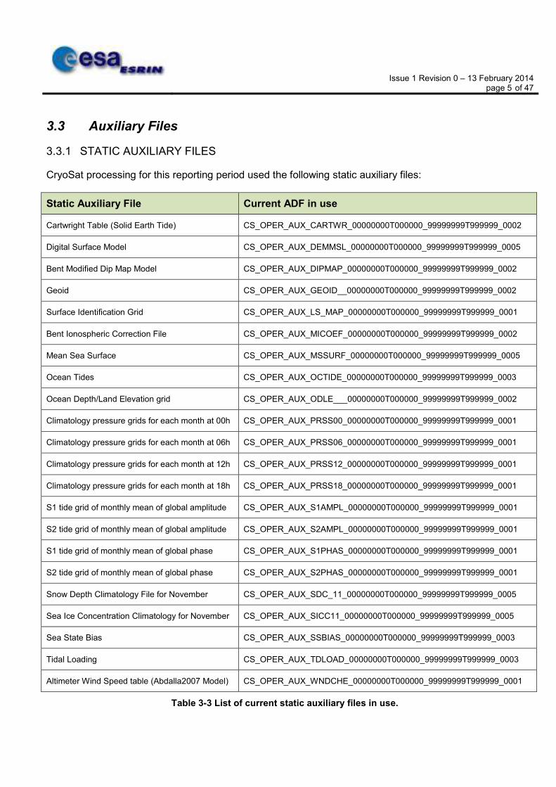
CryoSat processing for this reporting period used the following static auxiliary files:

Static Auxiliary File Current ADF in use

Cartwright Table (Solid Earth Tide) CS_OPER_AUX_CARTWR_00000000T000000_99999999T999999_0002

Digital Surface Model CS_OPER_AUX_DEMMSL_00000000T000000_99999999T999999_0005

Bent Modified Dip Map Model CS_OPER_AUX_DIPMAP_00000000T000000_99999999T999999_0002

Geoid CS_OPER_AUX_GEOID__00000000T000000_99999999T999999_0002

Surface Identification Grid CS_OPER_AUX_LS_MAP_00000000T000000_99999999T999999_0001

Bent Ionospheric Correction File CS_OPER_AUX_MICOEF_00000000T000000_99999999T999999_0002

Mean Sea Surface CS_OPER_AUX_MSSURF_00000000T000000_99999999T999999_0005

Ocean Tides CS_OPER_AUX_OCTIDE_00000000T000000_99999999T999999_0003

Ocean Depth/Land Elevation grid CS_OPER_AUX_ODLE___00000000T000000_99999999T999999_0002

Climatology pressure grids for each month at 00h CS_OPER_AUX_PRSS00_00000000T000000_99999999T999999_0001




S1 tide grid of monthly mean of global amplitude CS_OPER_AUX_S1AMPL_00000000T000000_99999999T999999_0001

S2 tide grid of monthly mean of global amplitude CS_OPER_AUX_S2AMPL_00000000T000000_99999999T999999_0001

S1 tide grid of monthly mean of global phase CS_OPER_AUX_S1PHAS_00000000T000000_99999999T999999_0001

S2 tide grid of monthly mean of global phase CS_OPER_AUX_S2PHAS_00000000T000000_99999999T999999_0001

Snow Depth Climatology File for November CS_OPER_AUX_SDC_11_00000000T000000_99999999T999999_0005

Sea Ice Concentration Climatology for November CS_OPER_AUX_SICC11_00000000T000000_99999999T999999_0005

Sea State Bias CS_OPER_AUX_SSBIAS_00000000T000000_99999999T999999_0003

Tidal Loading CS_OPER_AUX_TDLOAD_00000000T000000_99999999T999999_0003

Altimeter Wind Speed table (Abdalla2007 Model) CS_OPER_AUX_WNDCHE_00000000T000000_99999999T999999_0001

Table 3-3 List of current static auxiliary files in use.


3.3.2 DYNAMIC AUXILIARY FILES

CryoSat processing for this reporting period also used the following dynamic auxiliary files:

Dynamic Auxiliary File Current ADF in use

Solar Activity Index CS_OPER_AUX_SUNACT_19910101T000000_20141201T000000_0001

Gaussian Altimetric Grid CS_OPER_AUX_ALTGRD_20110504T100000_20301231T235959_0002

GPS Ionospheric Map CS_OPER_AUX_IONGIM_YYYYMMDDT000000_YYYYMMDDT235959

Updated daily

Polar Location CS_OPER_AUX_POLLOC_19870101T000000_YYYYMMDDT000000

Updated twice a week

Wet Troposphere CS_OPER_AUX_WETTRP_YYYYMMDDTxx0000_YYYYMMDDTxx0000

Meteo File *

Wind U-component CS_OPER_AUX_U_WIND_ YYYYMMDDTxx0000_YYYYMMDDTxx0000

Meteo File *

Wind V-component CS_OPER_AUX_V_WIND_ YYYYMMDDTxx0000_YYYYMMDDTxx0000

Meteo File *

Surface Pressure CS_OPER_AUX_SURFP_ YYYYMMDDTxx0000_YYYYMMDDTxx0000

Meteo File *

Sea Mean Pressure CS_OPER_AUX_SEAMPS_ YYYYMMDDTxx0000_YYYYMMDDTxx0000

Meteo File *

Dynamic Atmospheric Correction CS_OPER_AUX_MOG_2D_ YYYYMMDDTxx0000_YYYYMMDDTxx0000

Meteo File *

Dynamic Sea Ice Concentration CS_OPER_AUX_SEA_IC_YYYYMMDDT000000_YYYYMMDDT235959

Updated every 3 days

Table 3-4 List of dynamic auxiliary files in use.

*Meteo files are provided daily for each 6 hour grid (00h, 06h, 12h and 18h). Each product requires at least two, or sometimes three, of each Meteo file from the two grids between which the product validity lies.

3.3.3 CHANGES OF AUXILIARY FILES DURING THE CYCLE During the reporting period, there were no static auxiliary file updates.


4 PDS STATUS

4.1 SIRAL Instrument Unavailability The following unavailability periods have been noted for SIRAL data during this cycle:

UTC Start UTC Stop Reason Planned

2013-11-01 08:46:42 2013-11-01 09:48:14 Orbit Manoeuvre Yes

2013-11-15 04:21:36 2013-11-15 06:07:21 Orbit Manoeuvre Yes

Table 4-1 SIRAL instrument unavailability periods for cycle 38.

The historic list of all SIRAL data unavailability periods is available online at: http://earth.eo.esa.int/missions/cryosat/unavailability_periods/. The following sections provide information on the percentage of Level 0 (L0), L1B and L2 products, FDM and Offline, which have been successfully processed and made available. The information in Figure 4-1, Figure 4-2 and Figure 4-3 is extracted daily from the CryoSat Monitoring Facility (MF) and forms part of the routine data quality checks which are carried out to monitor data production. The availability of each level of data is calculated with respect to the available data from the preceding processing level.

4.2 SIRAL Level 0 Data Availability

Figure 4-1 SIRAL L0 Data Availability for cycle 38.

SIRAL L0 data was available at all times throughout this cycle, except for those periods listed in Table 4-1 when the instrument was unavailable due to planned or unplanned activities.


4.3 SIRAL Level 1B and Level 2 FDM Data Availability The availability of all L1B and L2 FDM mode data products for each day throughout this cycle is provided in Figure 4-2.

Figure 4-2 SIRAL L1B and L2 FDM Data Availability for cycle 38.

The percentage of L1B and L2 FDM data products made available was >72% throughout this reporting period. From the 18th- 26th November 2013 approximately 25% of L1B products were affected by a problem with the star tracker causing the corresponding L2 FDM products to fail.


4.4 SIRAL Level 1B and Level 2 Offline Data Availability The availability of all L1B and L2 offline data products for each day throughout this cycle is provided in Figure 4-3.

Figure 4-3 SIRAL L1B and L2 Offline Data Availability for cycle 38.

The percentage of L1B and L2 Offline Science data products made available was >92% throughout this reporting period. From the 18th- 26th November 2013 approximately 25% of L2 LRM products are missing due to failed FDM processing orders (see above).


5 SIRAL HEALTH MONITORING Various SIRAL parameters extracted from the L0 and the Monitoring Data Products are monitored on a daily basis in order to check the health and status of the SIRAL instrument.

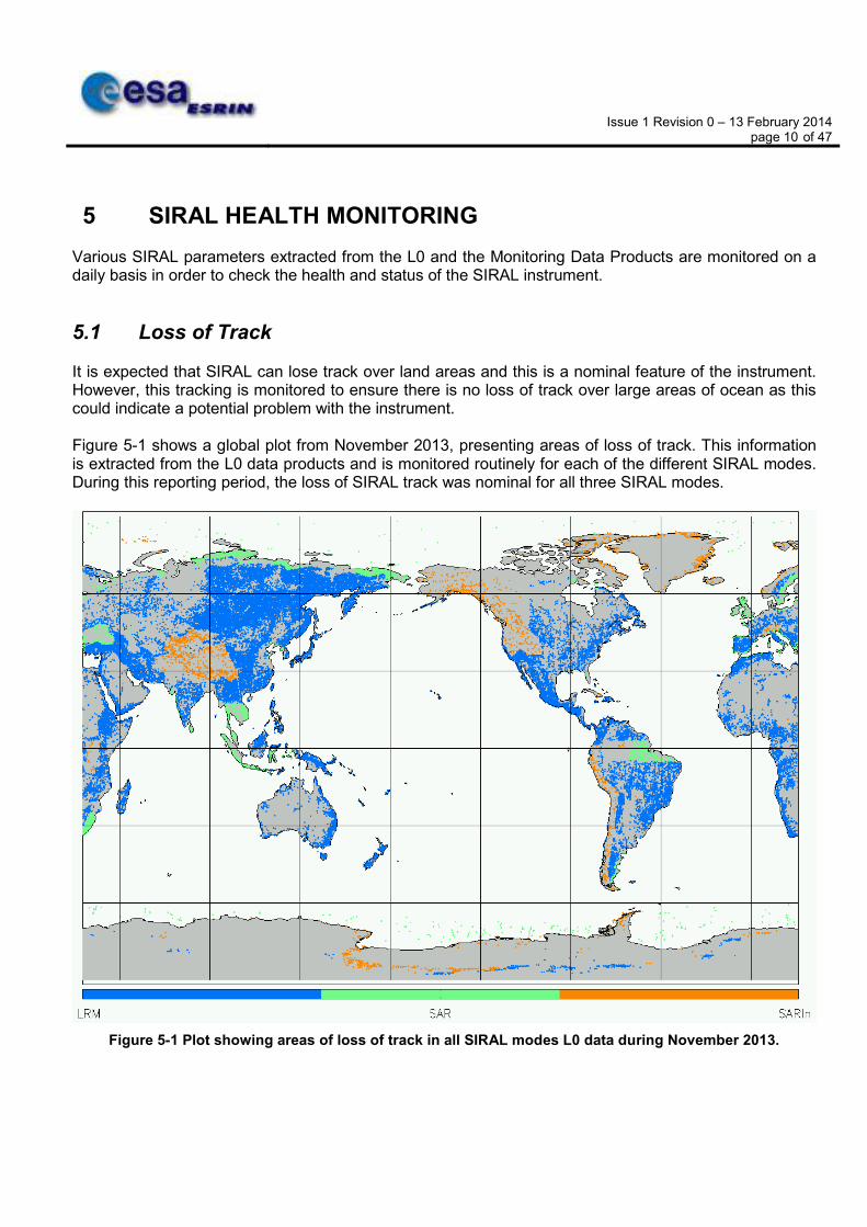
5.1 Loss of Track It is expected that SIRAL can lose track over land areas and this is a nominal feature of the instrument. However, this tracking is monitored to ensure there is no loss of track over large areas of ocean as this could indicate a potential problem with the instrument. Figure 5-1 shows a global plot from November 2013, presenting areas of loss of track. This information is extracted from the L0 data products and is monitored routinely for each of the different SIRAL modes. During this reporting period, the loss of SIRAL track was nominal for all three SIRAL modes.

Figure 5-1 Plot showing areas of loss of track in all SIRAL modes L0 data during November 2013.


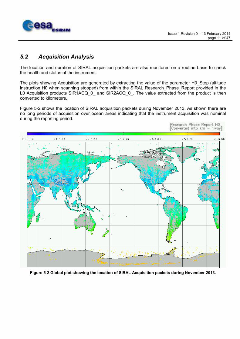
5.2 Acquisition Analysis The location and duration of SIRAL acquisition packets are also monitored on a routine basis to check the health and status of the instrument. The plots showing Acquisition are generated by extracting the value of the parameter H0_Stop (altitude instruction H0 when scanning stopped) from within the SIRAL Research_Phase_Report provided in the L0 Acquisition products SIR1ACQ_0_ and SIR2ACQ_0_. The value extracted from the product is then converted to kilometers. Figure 5-2 shows the location of SIRAL acquisition packets during November 2013. As shown there are no long periods of acquisition over ocean areas indicating that the instrument acquisition was nominal during the reporting period.

Figure 5-2 Global plot showing the location of SIRAL Acquisition packets during November 2013.


6 FDM DATA QUALITY CONTROL

6.1 Product Format Checks

As part of the Quality Control activities, a check is conducted to ensure that all expected L1B and L2 FDM data products have been generated with the correct format and that each CryoSat product is composed of two files; XML Header (.HDR) and Product File (.DBL).

Product Filename Format Check Discrepancy

None N/A

During cycle 38, there were no product format errors detected through this check.

6.2 Software Version Checks As part of the Quality Control activities, a check is conducted to ensure that all CryoSat FDM data products have been generated with the correct software version, listed in Table 3-1 and Table 3-2.

Product Filename Incorrect SW version detected

None N/A

During cycle 38, there were no software version errors detected through this check.

6.3 Forecast Auxiliary Data File Usage Checks All L1B and L2 FDM data products are routinely checked to ensure the process has used all the relevant forecast auxiliary data files in order to provide all the necessary geophysical corrections.

Product Filename Missing auxiliary correction

All products from 20131128T000103 to 20131128T235716 (162 L1B and 161 L2 FDM products)

Ionospheric


Ionospheric


Ionospheric

During cycle 38, there were 482 L1B and 478 L2 FDM products flagged through this check.


6.4 External Forecast Auxiliary Corrections Surface Height measurements, which are provided in the SIRAL L2 products, are corrected for atmospheric propagation delays and geophysical surface variations. For FDM products, forecast Auxiliary Data Files are used to provide the Meteo corrections for higher level processing. This section provides global maps of the value of each correction for cycle 38. All FDM products processed without the Meteo Auxiliary Data Files have been omitted from the generation of plots in the following sections. This may be due to the unavailability of Forecast Auxiliary Files at the time of the higher level FDM processing. Please refer to Section 6.3 for a list of these products.

6.4.1 DRY TROPOSPHERIC CORRECTION This is the correction for the path delay in the radar return signal due to the dry gas component of the atmosphere. For CryoSat FDM processing the Dry Tropospheric Correction is computed using forecast auxiliary files as inputs. Figure 6-1 shows, geographically, the value of the Forecast Dry Tropospheric Correction, applied to the L2 FDM data during cycle 38.

Figure 6-1 Global plot of the Forecast Dry Tropospheric Correction for cycle 38.


6.4.2 WET TROPOSPHERIC CORRECTION The Wet Troposphere Correction corrects for the path delay in the radar return signal due to liquid water in the atmosphere. For CryoSat FDM processing the Wet Tropospheric Correction is computed using forecast auxiliary files as inputs. Figure 6-2 shows, geographically, the value of the Forecast Wet Tropospheric Correction, applied to the L2 FDM data during cycle 38.

Figure 6-2 Global plot for the Forecast Wet Tropospheric Correction for cycle 38.


6.4.3 INVERSE BAROMETRIC CORRECTION The Inverse Barometric Correction compensates for variations in sea surface height due to atmospheric pressure variations, which is known as atmospheric loading. For CryoSat FDM processing the Inverse Barometric Correction is computed using forecast auxiliary files as inputs. While the Dynamic Atmospheric Correction (DAC) is nominally provided over the ocean, the MOG_2D forecast auxiliary files, used to provide the DAC, are not received by the PDS in time for higher level FDM processing. As a result the Inverse Barometric Correction is used instead. Figure 6-3 shows, geographically, the value of the Forecast Inverse Barometric Correction applied to the L2 FDM data during cycle 38.

Figure 6-3 Global plot for the Forecast Inverse Barometric Correction for cycle 38.


6.4.4 IONOSPHERIC CORRECTION The Ionospheric Correction compensates for the free electrons in the Earth's ionosphere slowing the radar pulse. Solar control of the ionosphere leads to geographic and temporal variations in the free electron content, which can be modelled or measured, for example, using the GPS satellite network. There are two sources currently used to derive this correction for CryoSat: the Global Ionospheric Map (GIM) and the Bent model. The GIM correction uses GPS measurements and is sourced from CNES via SSALTO as a dynamic daily forecast file. The Bent Model is derived from a static file and is based on knowledge of a solar activity index, such as sunspots. For CryoSat FDM processing the Ionospheric Correction is computed using forecast inputs for the GIM. If this is unavailable at the time of higher level FDM processing, the Bent model is used instead to provide this correction. Figure 6-4 shows, geographically, the value of the Ionospheric Correction applied to the L2 data during cycle 38.

Figure 6-4 Global plot for the Forecast Ionospheric Correction for cycle 38.


6.4.5 SEA STATE BIAS CORRECTION The Sea State Bias (SSB) Correction, also known at the Electromagnetic Bias Correction, is an empirical correction proportional to the significant wave height which compensates for the asymmetrical shape of ocean waves. Figure 6-5 shows, geographically, the value of the SSB Correction applied to the L2 FDM data during cycle 38.

Figure 6-5 Global plot of the Forecast SSB Correction for cycle 38.

Areas shown in red (zero) have the SSB Correction set to the default value of ‘32767’ as no SSB Correction is provided over land.


7 OFFLINE DATA QUALITY CONTROL

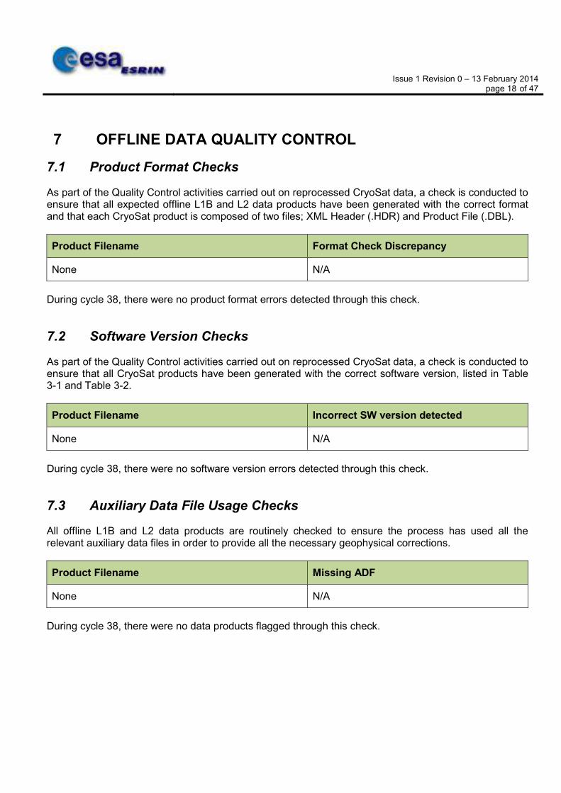
7.1 Product Format Checks As part of the Quality Control activities carried out on reprocessed CryoSat data, a check is conducted to ensure that all expected offline L1B and L2 data products have been generated with the correct format and that each CryoSat product is composed of two files; XML Header (.HDR) and Product File (.DBL).

Product Filename Format Check Discrepancy

None N/A

During cycle 38, there were no product format errors detected through this check.

7.2 Software Version Checks As part of the Quality Control activities carried out on reprocessed CryoSat data, a check is conducted to ensure that all CryoSat products have been generated with the correct software version, listed in Table 3-1 and Table 3-2.

Product Filename Incorrect SW version detected

None N/A

During cycle 38, there were no software version errors detected through this check.

7.3 Auxiliary Data File Usage Checks All offline L1B and L2 data products are routinely checked to ensure the process has used all the relevant auxiliary data files in order to provide all the necessary geophysical corrections.

Product Filename Missing ADF

None N/A

During cycle 38, there were no data products flagged through this check.


7.4 Product Parameters

7.4.1 MONITORING OF SIRAL MODE CHANGES CryoSat is designed to acquire continuously whilst switching automatically between its three nominal measurement modes, LRM, SAR and SARIn, according to a Geographical Mode Mask. Additionally, if one SIRAL receiver chain should fail then the instrument can operate in SARIn mode with one channel and this is referred to as SARIn Degraded (SID) mode. As the mode mask is updated regularly primarily to account for changes in sea-ice extent, between the different CryoSat cycles changes are expected in the SAR and LRM mode extents in areas of sea-ice. Figure 7-1 shows the daily percentages of each SIRAL mode for cycle 38. Further trends on both a cyclic and weekly basis are available on the MSSL Quality Monitoring website: http://cryosat.mssl.ucl.ac.uk/qa/view_mode_trend.php?dtlength=7.

Figure 7-1 Daily percentages of SIRAL modes for cycle 38.


Figure 7-2 shows global and polar plots of the SIRAL Modes acquired during cycle 38. These plots are generated from offline L2 Geophysical Data Record (GDR) data, which includes a SIRAL mode indicator for each 20 Hz record.

Figure 7-2 Global and Polar plots of SIRAL Modes for cycle 38.


7.4.2 SURFACE TYPE Figure 7-3 shows the surface type for cycle 38 over a global plot. The data is extracted from the offline L2 data products, which includes a surface type flag. The bit values of this flag provide a classification for the different surface type at nadir for the corresponding measurement location. The classification originates from a model provided by the ESA Geophysical CFI library.

Figure 7-3 Global plot of Surface Type for cycle 38.

% Open Ocean % Land % Continental Ice % Enclosed Sea % Unknown

69.53 20.35 9.77 0.33 0.02

Table 7-1 Surface Type statistics for cycle 38.


7.4.3 BACKSCATTER (SIGMA0) Each 20 Hz measurement record includes a radar backscatter (sigma0) value which provides information about the observed surface. It is a function of the radar frequency, polarisation and incidence angle and the target surface roughness, geometric shape and dielectric properties. Figure 7-4 shows global and polar plots of this parameter for cycle 38, for all three offline SIRAL modes. At L2, the backscatter coefficient is fully corrected, including instrument gain corrections and bias.

Figure 7-4 Global and Polar plots of Backscatter for cycle 38.


Figure 7-5, Figure 7-6 and Figure 7-7 below provide histograms for the Backscatter (sigma0) parameter, for each of the SIRAL modes.

Figure 7-5 Backscatter Histogram for LRM, cycle 38.

Figure 7-6 Backscatter Histogram for SAR, cycle 38.


Figure 7-7 Backscatter Histogram for SARIn, cycle 38.

It has been noted that in recent months backscatter values have been declining by ~0.1 dB per month. The power level transmitted by SIRAL has also been declining by a few 100ths of a dB per month. Nominally the CAL1 mode detects this and provides a correction to the sigma0 values, however there is currently an Anomaly Report (AR) open on this issue as this CAL1 correction is currently being applied with the wrong sign, hence the apparent drop in power. This problem is currently under investigation but CryoSat data users should be aware as this can in turn affect wind speed and sea state bias correction values.


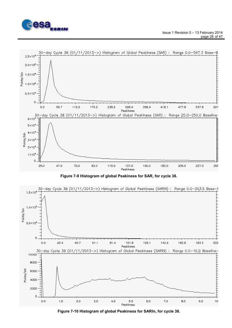
7.4.4 WAVEFORM PEAKINESS CryoSat offline L2 data includes a Waveform Peakiness value (field 39) for each 20 Hz measurement record. Peakiness is a ratio of the maximum waveform sample (bin) value to the mean value of the bins to the right of the tracking point. It is used to discriminate specular returns from diffuse returns and is used to estimate sea ice thickness. Figure 7-8, Figure 7-9 and Figure 7-10 below provide global Peakiness histograms for each of the SIRAL modes.

Figure 7-8 Histogram of global Peakiness for LRM, for cycle 38.


Figure 7-9 Histogram of global Peakiness for SAR, for cycle 38.

Figure 7-10 Histogram of global Peakiness for SARIn, for cycle 38.


Figure 7-11 shows the Waveform Peakiness for cycle 38, plotted over global and polar plots.

Figure 7-11 Global and Polar plots of Waveform Peakiness for cycle 38.


7.4.5 FREEBOARD CryoSat L2 data also includes a calculation for the Sea Ice Freeboard, which is the height by which an ice floe extends above the mean sea surface. This value can possibly be negative if there is heavy snow load on thin ice. At L2 it is calculated using UCL04 model values for snow depth and density. Presently, the freeboard values are not computed and a default value of -9999 is provided in the products by specification. The freeboard will be computed in the L2 products when there is a greater confidence in the knowledge of the Artic Mean Sea Surface with the launch of the SIR_SAR_2B and SIR_GDR_2B products.

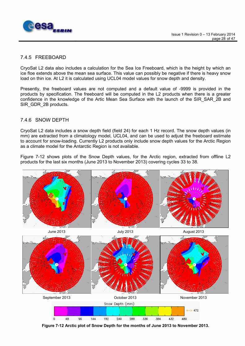
7.4.6 SNOW DEPTH CryoSat L2 data includes a snow depth field (field 24) for each 1 Hz record. The snow depth values (in mm) are extracted from a climatology model, UCL04, and can be used to adjust the freeboard estimate to account for snow-loading. Currently L2 products only include snow depth values for the Arctic Region as a climate model for the Antarctic Region is not available. Figure 7-12 shows plots of the Snow Depth values, for the Arctic region, extracted from offline L2 products for the last six months (June 2013 to November 2013) covering cycles 33 to 38.

Figure 7-12 Arctic plot of Snow Depth for the months of June 2013 to November 2013.

June 2013 July 2013 August 2013

October 2013 November 2013 September 2013


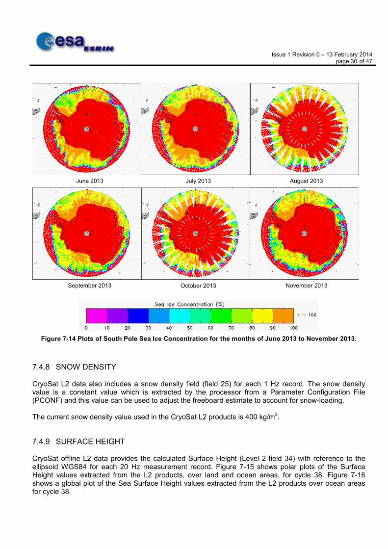
7.4.7 SEA ICE CONCENTRATION CryoSat L2 data includes a percentage value for the sea ice concentration field (field 23) for each 1 Hz record. Figure 7-13 and Figure 7-14 show the Sea Ice Concentration values extracted from the offline L2 products for the last six months (June 2013 to November 2013) covering cycles 33 to 38.

Figure 7-13 Plots of North Pole Sea Ice Concentration for the months of June 2013 to November 2013.




Figure 7-14 Plots of South Pole Sea Ice Concentration for the months of June 2013 to November 2013.

7.4.8 SNOW DENSITY CryoSat L2 data also includes a snow density field (field 25) for each 1 Hz record. The snow density value is a constant value which is extracted by the processor from a Parameter Configuration File (PCONF) and this value can be used to adjust the freeboard estimate to account for snow-loading. The current snow density value used in the CryoSat L2 products is 400 kg/m3.

7.4.9 SURFACE HEIGHT CryoSat offline L2 data provides the calculated Surface Height (Level 2 field 34) with reference to the ellipsoid WGS84 for each 20 Hz measurement record. Figure 7-15 shows polar plots of the Surface Height values extracted from the L2 products, over land and ocean areas, for cycle 38. Figure 7-16 shows a global plot of the Sea Surface Height values extracted from the L2 products over ocean areas for cycle 38.




Figure 7-15 Polar plots of Surface Height over land and ocean areas for cycle 38.

Figure 7-16 Global plots of Sea Surface Height for cycle 38.


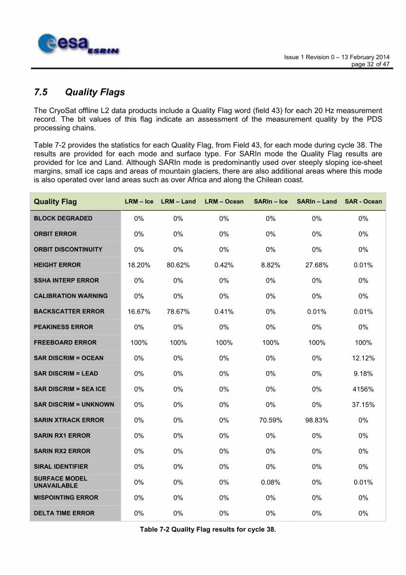
7.5 Quality Flags The CryoSat offline L2 data products include a Quality Flag word (field 43) for each 20 Hz measurement record. The bit values of this flag indicate an assessment of the measurement quality by the PDS processing chains. Table 7-2 provides the statistics for each Quality Flag, from Field 43, for each mode during cycle 38. The results are provided for each mode and surface type. For SARIn mode the Quality Flag results are provided for Ice and Land. Although SARIn mode is predominantly used over steeply sloping ice-sheet margins, small ice caps and areas of mountain glaciers, there are also additional areas where this mode is also operated over land areas such as over Africa and along the Chilean coast.

Quality Flag LRM – Ice LRM – Land LRM – Ocean SARIn – Ice SARIn – Land SAR - Ocean

BLOCK DEGRADED 0% 0% 0% 0% 0% 0%

ORBIT ERROR 0% 0% 0% 0% 0% 0%

ORBIT DISCONTINUITY 0% 0% 0% 0% 0% 0%

HEIGHT ERROR 18.20% 80.62% 0.42% 8.82% 27.68% 0.01%

SSHA INTERP ERROR 0% 0% 0% 0% 0% 0%

CALIBRATION WARNING 0% 0% 0% 0% 0% 0%

BACKSCATTER ERROR 16.67% 78.67% 0.41% 0% 0.01% 0.01%

PEAKINESS ERROR 0% 0% 0% 0% 0% 0%

FREEBOARD ERROR 100% 100% 100% 100% 100% 100%

SAR DISCRIM = OCEAN 0% 0% 0% 0% 0% 12.12%

SAR DISCRIM = LEAD 0% 0% 0% 0% 0% 9.18%

SAR DISCRIM = SEA ICE 0% 0% 0% 0% 0% 4156%

SAR DISCRIM = UNKNOWN 0% 0% 0% 0% 0% 37.15%

SARIN XTRACK ERROR 0% 0% 0% 70.59% 98.83% 0%

SARIN RX1 ERROR 0% 0% 0% 0% 0% 0%

SARIN RX2 ERROR 0% 0% 0% 0% 0% 0%

SIRAL IDENTIFIER 0% 0% 0% 0% 0% 0%

SURFACE MODEL UNAVAILABLE

0% 0% 0% 0.08% 0% 0.01%

MISPOINTING ERROR 0% 0% 0% 0% 0% 0%

DELTA TIME ERROR 0% 0% 0% 0% 0% 0%

Table 7-2 Quality Flag results for cycle 38.


Currently the Quality Flag for ‘Freeboard Error’ is set in all products as this parameter is currently not provided in the L2 products and the value is presently set to the default value of -9999 (please refer to section 7.4.5 for more details). It has been noted that the number of errors arising from the ‘Backscatter Error’ and ‘Height Error’ Quality Flag is much higher than expected over land-ice areas and this is currently part of an on-going investigation by expert teams. The SARIn Xtrack Error flag is used to indicate records flagged as ambiguous. In Level 2I SARin products, an Ambiguity Flag (field 73) is used to indicate ambiguity and is also used to indicate why the record has been flagged as ambiguous. Within the corresponding L2 SARIn products, there is only one bit available within the record structure to show this, so it is currently set if the difference between the computed surface elevation and the DEM is >50 m or if there isn't a DEM at the current location to check. As the DEM is only available for Greenland and Antarctica, the SARIn Xtrack flag can be ignored in all other regions. Currently there is an on-going investigation into the high number of errors from the ‘SARIn X-track Error’ Quality Flag over Antarctica.

7.6 Crossover Analysis This section provides results from crossover processing of offline L2 data from cycle 38.

7.6.1 CROSSOVER STATISTICS The crossover statistics for cycle 38, from each mode, is provided in Table 7-3 for Antarctica, Greenland and the Global Oceans.

Location Mode No of crossovers RMS Mean XTT Mean

Antarctica

LRM 45884 (62.7%) < 10.0 m 0.41 m -0.02 m 5.13 ms

SARIn 14990 (80.6%) < 10.0 m 1.91 m -0.02 m 0.39 ms

Greenland

LRM 375 (83.0%) < 1.0 m 0.35 m 0.19 m 15.82 ms

SARIn 1768 (65.5%) < 1.0 m 2.03 m -0.03 m -1.47 ms

Global Oceans LRM 9529 (94.8%) < 1.0 m 0.23 m -0.15 m 4.16 ms

Table 7-3 Cycle 38 Crossover statistics.


7.6.2 ELEVATION MAPS Figure 7-17 and Figure 7-18 show spatial polar maps of elevation differences at crossover per 10 km2 grid cells for L2 products from cycle 38. Over central Antarctica, there is an unexpected pattern which is clearly visible between -82 and -88 degrees. Crossover differences have a static and time varying component; this pattern is linked to the static component of the crossover difference and is meteorological in origin due to wind-induced features. The pattern can be removed by applying an elevation correction that is a function of the sigma0 crossover difference, see Armitage et al., 2013, “Meteorological Origin of the Static Crossover Pattern Present in Low-Resolution-Mode CryoSat-2 Data Over Central Antarctica”.

Figure 7-17 Greenland and Antarctica maps of LRM elevation differences for cycle 38.


Figure 7-18 Greenland and Antarctica maps of SARIn elevation differences for cycle 38.


7.6.3 BACKSCATTER (SIGMA0) MAPS Figure 7-19 and Figure 7-20 provide spatial polar maps of power differences at crossover per 10 km2 grid cells for L2 products from cycle 38. Over central Antarctica, there is an unexpected pattern which is clearly visible between -82 and -88 degrees. Crossover differences have a static and time varying component; this pattern is linked to the static component of the crossover difference and is meteorological in origin due to wind-induced features. The pattern can be removed by applying an elevation correction that is a function of the sigma0 crossover difference, see Armitage et al., 2013, “Meteorological Origin of the Static Crossover Pattern Present in Low-Resolution-Mode CryoSat-2 Data Over Central Antarctica”.

Figure 7-19 Greenland and Antarctica maps of LRM power differences for cycle 38.


Figure 7-20 Greenland and Antarctica maps of SARIn power differences for cycle 38.


7.7 External Auxiliary Corrections Surface Height measurements, which are provided in the SIRAL offline L2 products, are corrected for atmospheric propagation delays and geophysical surface variations. This section provides global maps of the value of each correction for cycle 38. Furthermore, the global trend taken from each 30-day cycle is also provided.

7.7.1 DRY TROPOSPHERIC CORRECTION This is the correction for the path delay in the radar return signal due to the dry gas component of the atmosphere. It has a typical range from 1.7 to 2.5 m. For CryoSat processing the Dry Tropospheric Correction is not provided via a specific auxiliary data file but is computed by the processors using ECMWF surface pressure files. Figure 7-21 shows, geographically, the value of the Dry Tropospheric Correction, applied to the L2 data during cycle 38. The global RMS value of this correction for this cycle is 2214 mm and Figure 7-22 shows there has been very little change in this value from previous cycles.

Figure 7-21 Global plot of Dry Tropospheric Correction for cycle 38.


Figure 7-22 Dry Tropospheric Correction RMS value trend for each 30-day cycle.

7.7.2 WET TROPOSPHERIC CORRECTION The wet troposphere correction is the correction for the path delay in the radar return signal due to liquid water in the atmosphere. It is calculated from radiometer measurements and meteorological models and has a typical range from 0 to 50 cm. Unlike the Dry Tropospheric Correction, the Wet Tropospheric Correction is retrieved directly from ECMWF analysed grids. These correction files are then simply formatted to the CryoSat PDS file standard before being directly used in the processor. Figure 7-23 shows, geographically, the value of the Wet Tropospheric Correction, applied to the L2 data during cycle 38. The global RMS value of this correction for cycle 38 is 144 mm and Figure 7-24 shows there has been a small steady change from previous cycles.


Figure 7-23 Global plot of Wet Tropospheric Correction for cycle 38.

Figure 7-24 Wet Tropospheric Correction RMS value trend for each 30-day cycle.


7.7.3 INVERSE BAROMETRIC CORRECTION The Inverse Barometric Correction compensates for variations in sea surface height due to atmospheric pressure variations, which is known as atmospheric loading. It has a typical range from ‐15 to +15 cm, and is calculated from data provided by Meteo France via the CNES SSALTO system. This correction is only used over sea ice and when the surface type is ‘open ocean’ in SAR mode offline data. Figure 7-25 shows, geographically, the value of the Inverse Barometric Correction applied to the L2 SAR data during cycle 38. The global RMS value of this correction for cycle 38 is 188 mm.

Figure 7-25 Global plot of Inverse Barometric Correction for cycle 38.

Figure 7-26 shows that, although there have been steady changes over the global oceans, the value of the correction in the Antarctic Ocean has varied more greatly between cycles. This greater variability in the south polar oceans is due to greater atmospheric pressure variability and hence sea level pressure variability. The Arctic Ocean, on the other hand, is more of an enclosed sea which explains the lower Inverse Barometric Correction values compared to the Antarctic values.


Figure 7-26 Inverse Barometric Correction RMS value trend for each 30-day cycle.

7.7.4 DYNAMIC ATMOSPHERE CORRECTION The dynamic atmospheric correction compensates for variations in sea surface height due to atmospheric pressure and winds. It has a typical range from ‐15 to +15 cm and is taken from the MOG2D model data provided by Meteo France via the CNES SSALTO system. This correction is only used over ocean without sea‐ice cover and when the surface type is ‘open ocean’, in SARIn and LRM mode. Figure 7-27 shows, geographically, the value of the Dynamic Atmospheric Correction, computed and applied to the L2 data during cycle 38. The global RMS value of this correction for cycle 38 is 117 mm. Figure 7-28 shows there has been a small steady change from previous cycles.


Figure 7-27 Global plot of Dynamic Atmosphere Correction for cycle 38.

Figure 7-28 Dynamic Atmosphere Correction RMS value trend for each 30-day cycle.


7.7.5 IONOSPHERIC CORRECTION The Ionospheric Correction compensates for the free electrons in the Earth's ionosphere slowing the radar pulse. Solar control of the ionosphere leads to geographic and temporal variations in the free electron content, which can be modelled, or measured, for example using the GPS satellite network. There are two sources currently used to derive this correction for CryoSat, the GIM and the Bent model. The GIM correction uses GPS measurements and is sourced from CNES via SSALTO as a dynamic daily file. The Bent Model is derived from a static file and is based on knowledge of a solar activity index, such as sunspots. The correction has a typical range from 6 to 12 cm. CryoSat L1B products currently contain the Ionospheric Correction values derived from both the GIM and Bent Model. At L2, only the Ionospheric Correction value applied to the range is provided. This is nominally derived using the GIM by default, however when this is unavailable the Bent model is used as an alternative. Figure 7-29 shows, geographically, the value of the Ionospheric Correction applied to the offline L2 data during cycle 38. The global RMS value of this correction for cycle 38 is 154 mm.

Figure 7-29 Global plot of Ionospheric Correction for cycle 38.

Currently, the Bent Model does not provide values for latitudes >82 degrees. However, this should not affect the nominal science data as, during offline L2 processing, the Ionospheric Correction, as shown in Figure 7-29 and Figure 7-30, is taken from the GIM model by default and the Bent Model is only used as an alternative when this GIM is not available.


Figure 7-30 Ionospheric Correction RMS value trend for each 30-day cycle.


8 ANOMALY REPORTS An updated list of all known anomalies which have been opened and tracked on the IPF and affect the quality of the distributed data products, is provided at the link below: https://earth.esa.int/web/guest/missions/cryosat/product-status. This list of anomalies is complete and up to date as of 11 February 2014 and is updated on a regular basis.


9 README DOCUMENTS ON PERFORMANCE AND QUALITY This section lists any current readme documents or notifications which have been issued and are relevant to the quality of CryoSat data. There were no readme documents issued during the period covered by this cycle.