c� 2017 Shweta Jayant Patwa

!!!!!SURVIVABLE NETWORK DESIGN PROBLEMS WITH ELEMENT AND VERTEX

CONNECTIVITY REQUIREMENTS !!!!!BY

!SHWETA JAYANT PATWA !!!!!!!

THESIS !Submitted in partial fulfillment of the requirements

for the degree of Master of Science in Computer Science in the Graduate College of the

University of Illinois at Urbana-Champaign, 2017 !!!

Urbana, Illinois !!Adviser: ! Professor Chandra Chekuri

Abstract

In this thesis, we consider degree-bounded element-connectivity Survivable Network Design Problem

(Elem-SNDP) and degree-bounded Rooted k-outconnectivity Problem. We suggest bicriteria approximation

algorithms that are motivated by Ene and Vakilian’s work in [1] and Lau and Zhou’s work in [2]. The

algorithm follows the iterated rounding framework that has been used for these problems over the past

many years. This can be achieved by adding a restriction on which edges can be added to the solution in

any iteration of the iterated rounding algorithm. We wanted to investigate this approach in the context of

degree-bounded Elem-SNDP and degree-bounded Rooted k-outconnectivity because it helped simplify the

proof idea for edge-connectivity SNDP (EC-SNDP), while achieving approximation ratios that were as good

as the best known result.

Given a graph G = (V,E) with costs on edges, connectivity requirements between pairs of vertices and

degree constraints on vertices, the goal is to compute a minimum cost subgraph H of G that obeys the

connectivity requirements and satisfies the degree bounds on the vertices. In the case of element connectivity,

connectivity requirement r(uv) between vertices u and v represents the required number of element-disjoint

paths between the two vertices. The elements are made up of all the edges and unreliable vertices. This

way of defining connectivity models networks where links and nodes can both fail. For Elem-SNDP, our

algorithm outputs a solution that has cost at most 3OPT and the degree on each vertex v in the solution is at

most 19b(v)+7. In the context of rooted k-outconnectivity problem, connectivity requirement represents

the number of internally vertex-disjoint paths between vertices the root r and a vertex v. We extend our

approach for Elem-SNDP to the degree-bounded Rooted k-outconnectivity problem. Our algorithm for the

latter computes a solution that has cost at most 3OPT and the out-degree on each vertex v in the solution is

19b+(v)+7. In addition, the in-degree of vertex v is bounded above by b�(v)+5.

ii

To Mom, Dad, Bhaiya and Bhabhi.

iii

ACKNOWLEDGEMENTS

I would like to express my sincere gratitude to my advisor, Professor Chandra Chekuri, for his support and

encouragement. He has inspired me since the time I took an undergraduate course with him, and has set an

example of excellence as a researcher, mentor, instructor and role-model. I feel blessed to have found an

advisor who always took the time out to listen to the small problems and roadblocks that I faced along the

way to finishing this thesis. I am deeply grateful for his guidance and feedback, which have proved to be

invaluable in the growth of my knowledge and maturity as a researcher. Thank you for believing in me when

I was not sure myself.

I would also like to thank the students in the theory group at Unoversity of Illinois at Urbana-Champaign

(UIUC) for not only the many academic discussions, but also the meals, board games, movie nights, and many

other seemingly small memories that I will cherish forever. Taking courses and teaching would not have been

the same without them. The many long hours that I spent in my office would have been harder if it was not

for the students around me. I will miss the various, often random, discussions with Shalmoli, Chao, Hsien

and Kent, Chao’s worldview and sense of humor, Shalmoli’s constant encouragement and wisdom, food and

coffee runs with Alex, Charlie, Patrick, Spencer, Chao, Tana, Shant, Xilin, Sahand and Mitchell, among many

other things. I also want to thank other people, whose names I may have missed, for their friendship. Thank

you for making Urbana-Champaign a fun place. I am extremely grateful to UIUC for the last six years. Being

here has given me endless opporutinities to learn and grow, and it has become my home away from home.

Last but not the least, I want to thank my mom, dad, bhaiya and bhabhi for all their love and support. I

cannot imagine being where I am today without them. Words cannot describe how thankful I am for their

encouragement and faith in me. Thank you for inspiring me to follow my dreams. I would like to thank

my friends Snegha, Aarti, Stuti, Sakshi, Arunita, Ashwarya, Brandon and many others who supported me

through the tough times and were there to celebrate the good times.

iv

Table of Contents

Chapter 1 Introduction . . . . . . . . . . . . . . . . . . . . . . . . . . . . . . . . . . . . . . . . . . 1

1.1 Preliminaries . . . . . . . . . . . . . . . . . . . . . . . . . . . . . . . . . . . . . . . . . . 5

1.2 Organization and overview of contributions . . . . . . . . . . . . . . . . . . . . . . . . . . 7

Chapter 2 Degree-bounded element-connectivity SNDP . . . . . . . . . . . . . . . . . . . . . . . 8

2.1 Introduction . . . . . . . . . . . . . . . . . . . . . . . . . . . . . . . . . . . . . . . . . . . 8

2.1.1 Iterated rounding approach . . . . . . . . . . . . . . . . . . . . . . . . . . . . . . . 8

2.2 (3,19b(v)+7)-approximation algorithm . . . . . . . . . . . . . . . . . . . . . . . . . . . . 10

2.3 Proof of Theorem 2.4 . . . . . . . . . . . . . . . . . . . . . . . . . . . . . . . . . . . . . . 12

Chapter 3 Degree-bounded rooted k-outconnectivity problem . . . . . . . . . . . . . . . . . . . 21

3.1 Introduction . . . . . . . . . . . . . . . . . . . . . . . . . . . . . . . . . . . . . . . . . . . 21

3.1.1 Iterated rounding approach . . . . . . . . . . . . . . . . . . . . . . . . . . . . . . . 21

3.2 (3,19b+(v)+7)-approximation algorithm . . . . . . . . . . . . . . . . . . . . . . . . . . . 22

3.3 Proof of Theorem 3.4 . . . . . . . . . . . . . . . . . . . . . . . . . . . . . . . . . . . . . . 25

Chapter 4 Conclusions . . . . . . . . . . . . . . . . . . . . . . . . . . . . . . . . . . . . . . . . . . 33

References . . . . . . . . . . . . . . . . . . . . . . . . . . . . . . . . . . . . . . . . . . . . . . . . . . . . 35

v

Chapter 1

Introduction

Survivable network design problem (SNDP) is motivated by real-world networks, where we want to ensure

connectivity despite links or nodes failing. It is an important area in combinatorial optimization and

approximation algorithms, and has applications in the design of telecommunication and traffic networks,

VLSI chip design, etc. The input to a network design problem is typically an undirected or directed graph

G = (V,E) with non-negative costs on edges, given by c(e), and connectivity requirements r(uv) between

pairs of vertices u and v. The goal is to find a minimum weight subgraph, H, of the input graph G that satisfies

the given connectivity constraints. What makes the problem more interesting, as we will see later, is fixing

degree bounds on vertices. Some of the well studied problems in this area include minimum spanning tree

(MST), Steiner tree and forest, k-edge-connectivity, k-vertex-connectivity, Steiner network, etc.

Minimum spanning tree (MST) is one of the well-studied network design problems. The input to the

MST problem is an undirected graph G = (V,E) with costs on edges, and the goal is to find a minimum cost

tree connecting all the vertices. In terms of connectivity, this means that we want each pair of vertices to be

1-edge-connected, i.e., removing an edge from the resulting graph should render it disconnected. By Menger’s

theorem, this is equivalent to saying that we want at least one unit of flow crossing each non-trivial cut in the

graph with unit capacities on edges. Another important network design problem is the Steiner tree problem,

which has been studied extensively. Given a set of terminals R, the goal is to find a minimum-cost tree in

the input graph connecting all terminals. Note that it does not need to be a spanning tree in the given input

graph. The decision version of the Steiner tree problem is known to be NP-complete [3], so the optimization

problem is NP-hard. In the case that we add degree constraints to vertices, a reduction from the Hamiltonian

path problem is enough to show that it is NP-complete to decide if all the degree-bounds can be satisfied.

Thus, we need approximation algorithms to get past the barrier. In the case of minimum bounded degree

spanning tree problem (MBDST), we are also given a degree bound b(v) for each vertex v. Singh and Lau

in [4] give an algorithm that returns a solution with cost at most OPT and degree on each vertex v in the

solution is at most b(v)+1.

Some other SNDP problems include edge-connectivity and vertex-connectivity SNDP. When all the

connectivity requirements have the same value, say k, it means that our goal is to compute either a k-edge

connecteg graph or a k-vertex connected graph. These problems are known to be NP-Hard for k � 1 in

1

comparison to MST which has k = 1. It is useful to understand that in regards to flow for the k-vertex

connectivity problem, we have unit capacities on vertices instead of edges, and we want a flow of at least

k units to go between each pair of vertices. We discuss the more general settings of these problems, i.e.,

when the connectivity requirements can vary among different pairs of vertices, in the remainder of this thesis.

Since Boruvka’s algorithm, survivable network design problems have gathered a lot of attention and many

sophisticated techniques have come to light. Some of the well studied techniques include greedy algorithms,

primal-dual approach and iterative rounding approach. Over the last few decades, these techniques have

been extended to more general network design problems. Our main focus in this thesis will be on iterative

rounding and we refer the reader to [5] for a survey on the known techniques.

In the case of edge-connectivity SNDP, r(uv) is the number of edge-disjoint paths needed between pairs

of vertices u and v. A major breakthrough for generalized Steiner network problem was made by Jain in [6].

Jain’s iterated rounding algorithm for EC-SNDP (without degree constraints) gave a solution with cost 2OPT

by viewing EC-SNDP as a cut covering problem. It involved finding a basic optimal solution to the natural

LP (linear programming) relaxation and proving that such a solution satisifes a key property which allows us

to add some edges to the solution subgraph. The same thing can be said about the residual problem, provided

the requirement function belongs to a certain class of functions. Let us look at how this problem can be

modeled using a cut function f . According to Menger’s theorem, if H has at least f (S) = maxu2S,v2V�S

r(uv)

edges going across any cut (S,V �S), then H is a feasible solution. Thus, the problem becomes one where

we want an H that covers the set function f , i.e., |dH(S)|� f (S) for every S.

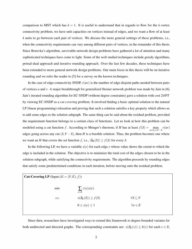
In the following LP, we have a variable x(e) for each edge e whose value shows the extent to which the

edge is included in the solution. The objective is to minimize the total cost of the edges chosen to be in the

solution subgraph, while satisfying the connectivity requirements. The algorithm proceeds by rounding edges

that satisfy some predetermined conditions in each iteration, before moving onto the residual problem.

Cut-Covering LP (Input:(G = (V,E), f ))

min Âe2E

c(e)x(e)

s.t. x(dE(S))� f (S) 8S✓V

0 x(e) 1 8e 2 E

Since then, researchers have investigated ways to extend this framework to degree-bounded variants for

both undirected and directed graphs. The corresponding constraints are: x(dE(v)) b(v) for each v 2 X ,

2

where X is the set of vertices with degree-bounds given by b(.). The trouble is that a simple reduction from

the Hamiltonian path problem can show that it is NP-complete to decide whether the degree constraints can

be satisfied. In addition, connectivity requirements act as covering constraints, whereas degree constraints act

as packing constraints. This was where bicriteria approximation algorithms came to the rescue. By relaxing

the degree constraints, Lau et al. in [7] and Lau and Singh in [8] were able to derive a good approximation

bound for degree-constrained EC-SNDP. Some examples of degree-bounded EC-SNDP are Hamiltonian path

problem and Traveling Salesman Problem (TSP).

In contrast to EC-SNDP, Elem-SNDP is concerned with element-disjoint paths between pairs of vertices.

The elements are made up of edges and unreliable vertices, i.e., nodes that can fail. Thus, it is only

reasonable that we want paths between pairs of vertices to not share elements because they can fail and disrupt

connectivity. Another variant of SNDP is vertex-connectivity SNDP (VC-SNDP). As the name suggests,

we want the the resulting subgraph to contain r(uv) number of internally vertex-disjoint paths between u

and v. Observe that Elem-SNDP can be viewed as lying somewhere in between EC-SNDP and VC-SNDP.

When the set of unreliable vertices is empty, Elem-SNDP reduces to EC-SNDP. Whereas, if u and v are

the only vertices with a connectivity requirement, then element-connectivity between them is the same as

vertex-connectivity between them.

Before we discuss some of the known results, let us see why EC-SNDP can be solved efficiently and

how researchers proved that it works. We know that the number of constraints in the LP is exponential in the

number of vertices, so why can we solve it in polynomial time? The key is that we need a polynomial time

separation oracle that can, given an extreme point solution x to the LP, either tell us that x is feasible or return

a violated constraint. What about the correctness and optimality of the iterated rounding algorithm? In each

iteration of the algorithm, we compute a basic solution to the LP, find edges that can be added to the solution

or degree constraints that can be dropped, and make the necessary updates to obtain the residual problem. It

is very important that the extreme point solution for the residual problem must also be a feasible solution to

the residual problem. The proof of correctness of such algorithms is contingent on a token counting argument

that can contradict the rank lemma for the LP. Thus, the iterative algorithm can be shown to return an optimal

solution using an inductive argument.

Let us first observe the notation used for convenience when describing approximation bounds of a

bicriteria approximation algorithm. For undirected graphs, an (a,bb(v) + g) bicriteria approximation

algorithm guarantees not only an a-approximation on the cost of H, but also that the degree of a vertex

v in H can be no more than bb(v)+ g . In the case that G is a directed graph, there are (a,bb+(v)+ g)

bicriteria approximation algorithms, where b+(v) represents the given out-degree constraints. In [7], Lau

3

et al. gave a (2,2b(v)+3)-approximation algorithm for EC-SNDP, i.e., an algorithm that returns a solution

with cost at most 2OPT such that the degree of any vertex v is at most 2b(v)+3. Whereas, [8] suggested an

additive approximation of b(v)+6rmax +3 for the degree bounds, where rmax is the maximum connectivity

requirement between any pair of vertices. More recently, Louis and Vishnoi in [9] showed that we can obtain

a (2,2b(v)+2)-approximation for EC-SNDP. The subtle difference between their algorithm and previous

algorithms is that b(v) can be kept integral or half-integral throughout the iterated rounding algorithm. What

if instead we could keep b(v) integral? Could that help simplify the token assignment and counting argument?

Indeed in [2], Lau and Zhou showed that by rounding edges, with x(e) at least 1/2 that are not incident to

any degree-constrained vertices, b(v) can remain integral. b(v) is updated only when an edge that is incident

to v and having x(e) = 1, is added to the solution. Fortunately, this idea also helped simplify and unify the

ideas for degree-bounded EC-SNDP. We refer the reader to [2] for details.

Despite being successful for EC-SNDP, the iterated rounding techniques from [7] and [8] could not prove

to be good enough for Elem-SNDP and VC-SNDP. In case of Elem-SNDP and VC-SNDP, it is not enough to

formulate the problem as a cut covering problem where we look at only the edges crossing a cut. Fleischer

et al. in [10] extended the iterated rounding framework to Elem-SNDP (without degree constraints) and

obtained an algorithm that computes a solution with cost 2OPT . Instead of defining the requirement function

f on a set, they defined it on a pair of sets, also called bisets. We discuss the related definitions and properties

that f must satisfy for Jain’s iterated rounding idea to work for Elem-SNDP in the next section. In [11],

Lau et al. show how similar techniques can be extended to VC-SNDP. For the degree constrained variants

of these two problems, Nutov’s results in [12] give an exponential dependence on rmax, also referred to as

k, for the degree violations. The paper gives an (O(logk),O(2k)b(v))-approximation algorithm for degree-

bounded Elem-SNDP and degree-bounded Rooted k-Connectivity. Recently, these results were improved

to have a linear dependence in k for degree violations. Fukunaga et al. in [13] derived an (O(k),O(k)b(v))-

approximation for Elem-SNDP and a (4,2b(v)+O(k)) for Rooted k-connectivity. In their joint work with

Nutov in [14], Fukunaga et al. improved upon their analysis to get an (O(1),O(1)b(v)+O(k))-approximation

for Elem-SNDP and (O(1),O(1)b+(v)+O(k))-approximation for Rooted k-outconnectivity problem. Ene

and Vakilian in [1] were the first to propose a constant factor approximation algorithm for degree-bounded

Elem-SNDP that promises a solution with cost at most three times that of the optimal and degree violation at

most 6b(v)+5 for vertex v. They consider the problem of covering a skew bisupermodular function using

iterated rounding, while taking advantage of the additional structure that this framework provides [1]. In the

same paper, they also obtain a (3,6b+(v)+3)-approximation for Rooted k-outconnectivity problem.

In this thesis, we discuss the degree-bounded versions of Elem-SNDP and Rooted k-outconnectivity

4

problem. Specifically, we closely follow the result from [1] and the condition on which heavy edges get

selected from [2], to propose a new algorithm. The motivation was that choosing heavy edges that are not

incident to any degree constrained vertices can ensure that b(v) stays integral. In the case of degree-bounded

EC-SNDP, this helped simplify the proof idea for the (2,2b(v)+ 2)-approximation in [2]. We wanted to

investigate how well such an algorithm can perform for degree-bounded Elem-SNDP and k-outconnectivity

problem. We believe that this approach seems promising and could lead to ,if not better, a bound that is

comparable to the best result known so far. To get a better idea of what other bounds might be provable for

our algorithm, we also investigated an O(1)b(v)+O(k)-approximation for the degree violations. However,

this involved extending the framework from sets to bisets (defined below), adding more technical difficulties

that prevented us from get positive results.

1.1 Preliminaries

This section covers important definitions and properties of biset functions that we need for the correctness

and optimality of our algorithm.

Bisets: Let V be a ground set. A biset A is defined as a pair of sets, (A,A0), such that A✓ A0 ✓V . A is called

the inner part of the biset whereas A0 is called the outer part of the biset. A0 �A is called the boundary of the

biset A and denoted by bd(A).

Figure 1.1. Example of a biset with vertex v in the inner part.

Suppose B= (B,B0) is another biset. The intersection of A and B is defined as A\B= (A\B,A0 \B0),

the union is defined as A[B= (A[B,A0 [B0) and the difference is defined as A�B= (A�B0,A0 �B). A

partial order ✓, or containment, on bisets is defined as follows. A✓ B if and only if A✓ B and A0 ✓ B0, i.e.,

5

B contains A. Thus, A\B✓ A,A\B✓ B,A�B✓ A and B�A✓ B.

Disjointness and bilaminarity: We discuss disjointness of bisets and bilaminarity of a family of bisets. Aand B are said to be disjoint when A\B is empty. Otherwise, they are said to be intersecting. In contrast, Aand B are strongly disjoint if A0 \B and B0 \A are both empty. If not, A and B are called overlapping. Now

consider a family of bisets. The family is called bilaminar if for every pair of bisets A and B in the family,

either A✓ B or B✓ A or A and B are disjoint. The family of bisets is called strongly bilaminar if for any two

bisets A and B in the family, either A✓ B or B✓ A or A and B are strongly disjoint.

Bisupermodularity and bisubmodularity: Let f be a function on bisets that is integer valued. The function

f is said to be bisupermodular if for any two bisets A and B,

f (A)+ f (B) f (A\B)+ f (A[B).

In the case that the inequality holds for any two intersecting bisets, f is referred to as intersecting bisupermod-

ular. f is called positively bisupermodular if the inequality holds for any two bisets A and B with f (A)> 0

and f (B)> 0. It is also known that f is bisubmodular if � f is bisupermodular.

The function f is binegamodular if for any two bisets A and B, we have that f (A)+ f (B) f (A�B)+f (B�A). If � f is binegamodular then f is biposimodular. Lastly, the function f is skew bisupermodular if

for any two bisets A and B,

f (A)+ f (B)max{ f (A\B)+ f (A[B), f (A�B)+ f (B�A)}.

Lastly, f is positively skew bisupermodular if the above inequality holds for bisets A and B with f (A)> 0

and f (B)> 0.

For a set of undirected edges F and a biset A, dF(A) is defined to be the set of edges which have an

endpoint in A and another endpoint in V �A0. The characteristic vector c(dF(A)) is defined to be an |F |-

dimensional vector with a 1 in the ith position if edge ei 2 dF(A), and 0 otherwise. In the case that F is a set

of directed edges, d�F (A) represents the edges with heads in A and tails outside A0, whereas d+F (A) is the set

of edges with heads outside A0 and tails in A. Here, the characteristic vector c(d�F (A)) is an |F |-dimensional

vector with a 1 in the ith position if edge ei 2 d�F (A), and 0 otherwise.

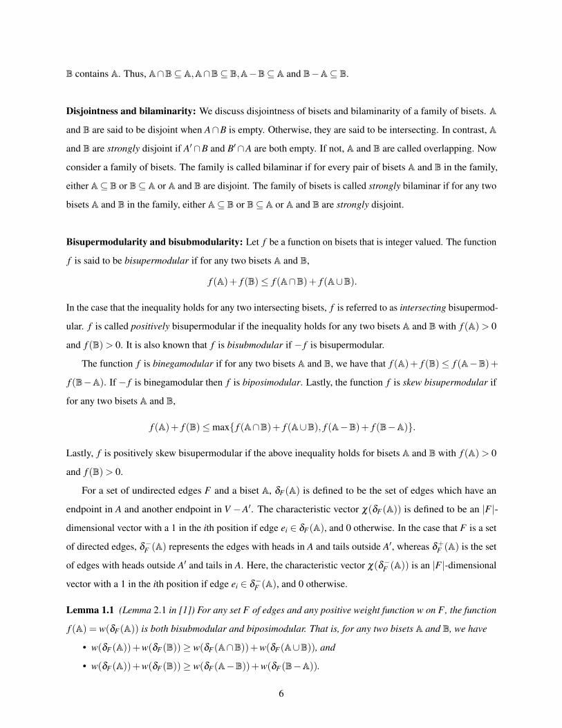
Lemma 1.1 (Lemma 2.1 in [1]) For any set F of edges and any positive weight function w on F, the function

f (A) = w(dF(A)) is both bisubmodular and biposimodular. That is, for any two bisets A and B, we have

• w(dF(A))+w(dF(B))� w(dF(A\B))+w(dF(A[B)), and

• w(dF(A))+w(dF(B))� w(dF(A�B))+w(dF(B�A)).

6

Lemma 1.2 (Lemma 2.2 in [1]) For any set F of directed edges and any positive weight function w on F,

the function f (A) = w(d�F (A)) is bisubmodular. That is, for any two bisets A and B, we have

w(d�F (A))+w(d�F (A))� w(d�F (A\B))+w(d�F (A[B)).

Lemma 1.3 (Lemma 2.3 in [1]) For any two bisets A and B,

• |bd(A)|+ |bd(B)|= |bd(A\B)|+ |bd(A[B)|, and

• |bd(A)|+ |bd(B)|= |bd(A�B)|+ |bd(B�A)|+2|bd(A)\bd(B)|.

1.2 Organization and overview of contributions

In this thesis, we discuss a new algorithm for degree-bounded Elem-SNDP and degree-bounded Rooted

k-outconnectivity problems. As mentioned earlier, our algorithm takes inspiration from [1]. We impose

an additional condition that only the heavy edges that are not incident to any degree-constrained vertex

can be added to the solution subgraph. In the case of EC-SNDP, this was enough to get a simplified, even

unified, algorithm and proof idea (see [2]). We were able to show that this can result in a (3,19b(v)+

7)-approximation for degree-bounded Elem-SNDP and a (3,19b+(v) + 7)-approximation for Rooted k-

outconnectivity. Chapters 2 and 3 talk about the details for these results. We believe that this approach could

potentially be useful in showing, if not better, a bound that is comparable to the best known result. In chapter

4 we try to shed light on whether a bound like (O(1),O(1)b(v)+O(k)) can be proved for the algorithm for

either problem. Borrowing ideas from other results involved extending the framework from sets to bisets, and

this posed additional technical difficulties.

7

Chapter 2

Degree-bounded element-connectivity SNDP

2.1 Introduction

In this chapter, we discuss degree-bounded Elem-SNDP. This problem deals with the scenario when edges

and some of the vertices can fail. The input is an undirected graph G = (V,E) with edge weights given

by c : E ! R+ and degree bounds given by b : V ! R�0. Additionally, V is partitioned into a set R of

reliable vertices and a set W of unreliable vertices. W and E together constitute elements. The connectivity

requirements are specified by r so that r(uv)> 0 only if u,v2 R. These specify the number of element-disjoint

paths needed between pairs of reliable vertices.

The goal is to find a minimum-weight subgraph H of G such that each pair of reliable vertices satisfies its

connectivity requirement and each vertex obeys its degree constraint. Note that the element-disjoint paths

cannot share unreliable vertices, but they can still share reliable vertices. G is said to cover the biset function

f if |dG(A)|� f (A) for each biset A. In the degree-bounded setting, we also want |dH(v)| b(v), for every

vertex in V .

Let relt be an integer-valued biset function given by relt(A) = maxu2A,v2V�A0 r(uv) if bd(A) ✓W , and

0 otherwise. Let felt be an integer-valued biset function given by felt(A) = relt(A)� |bd(A)| ( [1]). By

Menger’s theorem, a subgraph H satisifes the requirements if and only if |dH(A)|� felt(A) for each biset A,

i.e., if H covers felt .

Lemma 2.1 (Fleischer et al. [10]) The functions felt and relt are positively skew bisupermodular.

Recent work by Ene and Vakilian in [1] has led to a (3,6b(v)+5)-approximation for degree-bounded Elem-

SNDP. We take inspiration from their work and analyze what happens when we add restrictions to which

edges from the basic solution can be added to the solution in the iterated rounding algorithm. In the following

sections, we discuss important contributions made by the (3,6b(v)+5)-approximation algorithm from [1],

and present a different algorithm along with the details for the (3,19(v)+7)-approximation.

2.1.1 Iterated rounding approach

Consider an undirected graph G = (V,E). Let r and f be functions on bisets as described above, X be the set

of vertices with degree constraints and b(v) be the degree-bound for vertex v. Thus, LP for degree-bounded

8

Elem-SNDP on G is as follows:

Undir-LP (Input:(G = (V,E), f ,X ,b))

min Âe2E

c(e)x(e)

s.t. x(dE(A))� f (A) 8A : f (A)> 0

x(dE(v)) b(v) 8v 2 X

0 x(e) 1 8e 2 E

Once we have the above LP relaxation and a polynomial time separation oracle, we can solve the LP for

a basic optimal solution. Let x be such an extreme point solution. When proving the performance of the

algorithm, characterizing x by a sparse structure plays a crucial role. This often involves the standard

uncrossing technique. We will discuss this in further detail in the following sections of this chapter. The

iterated rounding algorithm relies on two steps: rounding and relaxation. Rounding is when we add heavy

edges from x to the solution subgraph. Relaxation helps mitigate the problem of having both covering and

packing constraints. Thus, if there is a vertex with small enough degree, which depends on the bound we

wish to prove, in x then we can remove the corresponding constraint in the residual LP formulation. Note that

it is possible that once a degree constrained vertex is dropped in the residual LP, edges incident to the same

vertex get added in the remaining iterations of the algorithm. Thus, this plays an important role in the analysis

of degree violations. We need to update x to reflect changes due to rounding and relaxation so that it stays

feasible for when applied to the residual problem. Following is a useful definition of the degree-bounded

residual cover problem.

Definition (Ene and Vakilian [1]) Degree-bounded Residual Cover: Let G = (V,E) be an undirected graph

with weights w(e) on the edges and degree bounds b(v) on the vertices. In the Degree-bounded Residual

Cover problem, we are given a function f : 2V ⇥ 2V ! Z satisfying f (A) = r(A)� |bd(A)|� |dF(A)| for

each biset A, where r is a biset function and F ✓ E is a set of edges, and the goal is to select a minimum

weight set F 0 ✓ E�F of edges such that |dF 0(A)|� f (A) for each biset A and |dF 0(v)| b(v) for each vertex

v.

The iterated rounding algorithm for the Degree-bounded Residual Cover problem in [1] gives an (O(1),

O(1)b(v))-approximation, as long as the requirement function r satisifes some technical conditions. The

following theorem elaborate the properties that the requirement and cut functions must satisfy.

9

Theorem 2.2 (Theorem 3.2 in [1]) Consider an instance of the Degree-bounded Residual Cover problems in

which the function f satisfies f (A) = r(A)� |bd(A)|� |dF(A)| for each biset A, where r is an integer-valued

biset function and F ✓ E is a set of edges. Let OPT be the weight of an optimal solution for the instance.

Suppose that r and f satisfy the following conditions:

• For each biset (A,A0) and each vertex v 2 A0 �A, we have r((A,A0)) r((A,A0 � v)).

• The function r is positively skew bisupermodular.

Then there is a polynomial time iterated rounding algorithm that selects a set F 0 ✓ E�F of edges such that

w(F 0) 3OPT and |dF 0(v)| |dF(v)|+6b(v)+5 for each vertex v.

It is known that felt and relt satisfy the technical conditions prescribed by the above theorem. The algorithm

for degree-bounded Elem-SNDP in [1] applies this theorem with F = /0, f = felt and r = relt , where felt and

relt are the functions defined previously. This gives the following result.

Theorem 2.3 (Theorem 3.3 in [1]) There is a polynomial time (3,6b(v)+5) approximation algorithm for

the degree-bounded Elem-SNDP problem in undirected graphs.

2.2 (3,19b(v)+7)-approximation algorithm

Given G = (V,E), r, f , X and b(v), the objective is to minimize the cost of the edges in the solution subject

to connectivity requirements and degree-bounds. Note that we are working with the LP relaxation, so we

let 0 x(e) 1 because we do not wish to have multiple copies of the same edge included in our solution.

For notational convenience, we define an edge e to be heavy in a basic feasible solution x if x(e) � 1/3.

Otherwise, the edge is called a light edge. We refer to edges as heavy or light throughout this thesis for

notational convenience.

Our algorithm is an iterated rounding algorithm. It works as follows: Each iteration of the while loop

starts with computing a basic optimal solution x to the LP relaxation for the (residual) graph. The success

of the remaining iteration, and therefore the overall algorithm, depends on there being either an edge e

with x(e) = 0 or 1, or there being a heavy edge which is not incident to any degree-bounded vertices, or

there being a degree-bounded vertex v with degree at most 18b(v)+ 7. If any of these conditions holds

true, the corresponding edge (or vertex) is either removed from the residual problem or the edge is added to

the solution subgraph. Remember that the degree-bounds need to be updated so that x stays feasible when

restricted to the residual problem. Hence, our main contribution is the following theorem which shows that

the algorithm must terminate.

Theorem 2.4 Consider an iteration of Undir-alg. Let G0 = (V,E 0) be the residual subgraph at the beginning

of this iteration. Let F 0 be the set of edges selected in the previous iterations. Let X 0 be the set of vertices

10

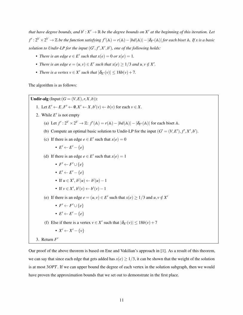
that have degree bounds, and b0 : X 0 ! R be the degree bounds on X 0 at the beginning of this iteration. Let

f 0 : 2V ⇥2V ! Z be the function satisfying f 0(A) = r(A)� |bd(A)|� |dF 0(A)| for each biset A. If x is a basic

solution to Undir-LP for the input (G0, f 0,X 0,b0), one of the following holds:

• There is an edge e 2 E 0 such that x(e) = 0 or x(e) = 1.

• There is an edge e = (u,v) 2 E 0 such that x(e)� 1/3 and u,v /2 X 0.

• There is a vertex v 2 X 0 such that |dE 0(v)| 18b(v)+7.

The algorithm is as follows:

Undir-alg (Input:(G = (V,E),r,X ,b)):

1. Let E 0 E,F 0 /0,X 0 X ,b0(v) b(v) for each v 2 X .

2. While E 0 is not empty

(a) Let f 0 : 2V ⇥2V ! Z: f 0(A) = r(A)� |bd(A)|� |dF 0(A)| for each biset A.

(b) Compute an optimal basic solution to Undir-LP for the input (G0 = (V,E 0), f 0,X 0,b0).

(c) If there is an edge e 2 E 0 such that x(e) = 0

• E 0 E 0 �{e}

(d) If there is an edge e 2 E 0 such that x(e) = 1

• F 0 F 0 [{e}

• E 0 E 0 �{e}

• If u 2 X 0, b0(u) b0(u)�1

• If v 2 X 0, b0(v) b0(v)�1

(e) If there is an edge e = (u,v) 2 E 0 such that x(e)� 1/3 and u,v /2 X 0

• F 0 F 0 [{e}

• E 0 E 0 �{e}

(f) Else if there is a vertex v 2 X 0 such that |dE 0(v)| 18b(v)+7

• X 0 X 0 �{v}

3. Return F 0

Our proof of the above theorem is based on Ene and Vakilian’s approach in [1]. As a result of this theorem,

we can say that since each edge that gets added has x(e)� 1/3, it can be shown that the weight of the solution

is at most 3OPT . If we can upper bound the degree of each vertex in the solution subgraph, then we would

have proven the approximation bounds that we set out to demonstrate in the first place.

11

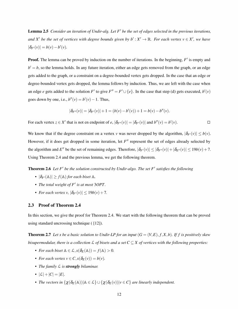
Lemma 2.5 Consider an iteration of Undir-alg. Let F 0 be the set of edges selected in the previous iterations,

and X 0 be the set of vertices with degree bounds given by b0 : X 0 ! R. For each vertex v 2 X 0, we have

|dF 0(v)|= b(v)�b0(v).

Proof. The lemma can be proved by induction on the number of iterations. In the beginning, F 0 is empty and

b0 = b, so the lemma holds. In any future iteration, either an edge gets removed from the graph, or an edge

gets added to the graph, or a constraint on a degree-bounded vertex gets dropped. In the case that an edge or

degree-bounded vertex gets dropped, the lemma follows by induction. Thus, we are left with the case when

an edge e gets added to the solution F 0 to give F 00 = F 0 [{e}. In the case that step (d) gets executed, b0(v)

goes down by one, i.e., b00(v) = b0(v)�1. Thus,

|dF 00(v)|= |dF 0(v)|+1 = (b(v)�b0(v))+1 = b(v)�b00(v).

For each vertex z 2 X 0 that is not en endpoint of e, |dF 00(v)|= |dF 0(v)| and b00(v) = b0(v). É

We know that if the degree constraint on a vertex v was never dropped by the algorithm, |dF 0(v)| b(v).

However, if it does get dropped in some iteration, let F 00 represent the set of edges already selected by

the algorithm and E 00 be the set of remaining edges. Therefore, |dF 0(v)| |dF 00(v)|+ |dE 00(v)| 19b(v)+7.

Using Theorem 2.4 and the previous lemma, we get the following theorem.

Theorem 2.6 Let F 0 be the solution constructed by Undir-algo. The set F 0 satisfies the following

• |dF 0(A)|� f (A) for each biset A.

• The total weight of F 0 is at most 3OPT .

• For each vertex v, |dF 0(v)| 19b(v)+7.

2.3 Proof of Theorem 2.4

In this section, we give the proof for Theorem 2.4. We start with the following theorem that can be proved

using standard uncrossing technique ( [12]).

Theorem 2.7 Let x be a basic solution to Undir-LP for an input (G = (V,E), f ,X ,b). If f is positively skew

bisupermodular, there is a collection L of bisets and a set C ✓ X of vertices with the following properties:

• For each biset A 2 L,x(dE(A)) = f (A)> 0.

• For each vertex v 2C,x(dE(v)) = b(v).

• The family L is strongly bilaminar.

• |L|+ |C|= |E|.

• The vectors in {c(dE(A))|A 2 L}[{c(dE(v))|v 2C} are linearly independent.

12

From Theorem 2.2, we know that f is positively skew bisupermodular. Using Lemma 1.1, we can conclude

that dF 0(.) is bisubmodular and biposimodular. This means that f 0 is also positively skew bisupermodular.

Thus, Theorem 2.7 can be applied to x and (G0 = (V,E 0), f 0,X 0,b0) to get a collection L of tight bisets and a

set C of tight vertices. We prove Theorem 2.4 by contradiction. Assume all of the following to be true:

• For every edge e, 0 < x(e)< 1.

• For any edge e, either x(e)� 1/3 and one of u or v is in X 0, or x(e)< 1/3.

• For every degree constrained vertex v 2 X 0, |dE 0(v)|� 18b(v)+8.

We assign two tokens for each edge in E 0, making the total number of tokens equal 2|E 0|. The goal here

is to prove that these tokens can be rearranged so that each biset in L gets at least two tokens, each vertex

in C gets at least two tokens, and each maximal biset in L gets at least four tokens. This would contradict

|E|= |L|+ |C| from Theorem 2.7.

To achieve this goal, we view L as a rooted forest based on biset-inclusion relation. A biset B is a child

of A if A 6= B and B✓ A and there is no biset C 2 L�{A,B} such that B✓ C✓ A; A is called the parent of

B. B is a descendent of A if B✓ A, whereas it is a proper descendent of A if B⇢ A. A biset is a leaf if it

does not have any children. A biset is a root if it is a maximal biset of L, i.e., it does not have a parent.

Here is an important definition about relevance of a biset for a vertex v and a property that the relevant

bisets satisfy. We care about the relevant bisets of degree-bounded vertices because they affect the token

assignment scheme.

Definition (Ene and Vakilian [1]) A bisetA2L is relevant for a vertex v2V if all of the following conditions

hold:

• A has one child.

• The vertex v is on the boundary of A but not on the boundary of the child of A.

Lemma 2.8 (Lemma 4.8 in [1]) Let v be a vertex in V . If L is a bilaminar family, the relevant bisets of v are

pairwise disjoint.

We use a token assignment that is similar to the one seen in section 5 from [1]. Any changes are marked

with a (⇤). The token assignment happens in two stages given by initial token assignment and first token

assignment, respectively. In the second token assignment, these tokens are reassigned among tight bisets and

tight degree-bounded vertices to get a contradiction. Let in(A) denote the set of edges with one endpoint in A

and the other endpoint in A0.

Initial token assignment: Each edge e = (u,v) 2 E 0 has two tokens te,u and te,v, one for each endpoint. The

edge e distributes te,u to L[C as follows (same rules apply to the token te,v):

13

• (Rule A) If u 2C, the token te,u is assigned to u.

• (Rule B) If u /2C, the token te,u is assigned to the minimal biset A= (A,A0) 2 L such that e 2 dE 0(A)and u 2 A.

If there does not exist such a biset, the token te,u is assigned to the minimal biset B which has

(u,v) 2 in(B).

First token assignment: After the initial token assignment, each vertex v in C gets |dE 0(v)| tokens. These

tokens get reassigned to bisets in L according to the following rules:

1. For each biset A 2 L that is relevant for v and has a unique child B 2 L:

(a) If dE 0(A)�dE 0(B) is empty and all edges in dE 0(B)�dE 0(A) are incident to v, v gives 2 tokens to

A.

(b) Otherwise, v gives min{1, |(dE 0(B)�dE 0(A))\dE 0(v)|} tokens to A.

2. For a minimal biset S 2 L with v 2C:

(a) (⇤) If S is a leaf, v gives 4 tokens to S.(b) If S is not a leaf and has a unique child T 2 L, v gives min{2, |((dE 0(S)� dE 0(T))[ (dE 0(T)�

dE 0(S)))\dE 0(v)|} tokens to S.

3. (⇤) For every heavy edge e = (u,v), if u is not degree-constrained but v is, v gives a token to u

(motivated by [2]). If u is in a leaf biset and x(e)� 2/3, then v gives another token to u.

These rules are designed so as to get a contradiction to Theorem 2.7. Recall that we assign two tokens per

edge, which brings the total number of tokens to 2|E|. Using the multi-stage token assignment scheme, we

wish to show that |L|+ |C| 6= |E|. The proof to the second token assignment discusses the many possible

cases in depth. But, before that, let us look at the following cases.

• The first case is when A has only one child B and v is a degree constrained vertex (in C). Moreover,

dE 0(A)�dE 0(B) is empty and all edges in dE 0(B)�dE 0(A) are incident to v. See figure 2.1 below. We

want A to get at least 4 tokens. However, it can get only 2 from B. If v could give 2 tokens to A, then

the main proof can go through for this scenario. This is the motivation for rules 1 (a) and (b).

• Now, consider the possibility when A is a leaf and has exactly one degree-bounded vertex v in the inner

part. All the edges incident to v are the ones that are also incident to the biset A. See figure 2.2 below.

Thus, in order for the proof to go through, we need v to give at least 4 tokens to A. Hence, we require

rule 2 (a). Rule 2 (b) is motivated from the same idea as rules 1 (a) and (b).

• Lastly, consider the case when A is a leaf and has 2 edges, e1 = (u,v) and e2, incident to it. Suppose

2/3 < x(e1)< 1 and x(e2) = 1� x(e1); f (A) = 1. Also, v is a degree-bounded but u is not. See figure

14

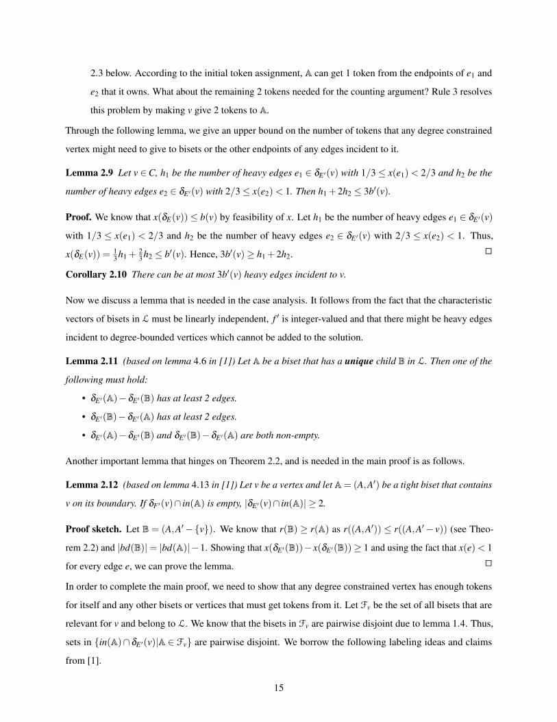
2.3 below. According to the initial token assignment, A can get 1 token from the endpoints of e1 and

e2 that it owns. What about the remaining 2 tokens needed for the counting argument? Rule 3 resolves

this problem by making v give 2 tokens to A.

Through the following lemma, we give an upper bound on the number of tokens that any degree constrained

vertex might need to give to bisets or the other endpoints of any edges incident to it.

Lemma 2.9 Let v 2C, h1 be the number of heavy edges e1 2 dE 0(v) with 1/3 x(e1)< 2/3 and h2 be the

number of heavy edges e2 2 dE 0(v) with 2/3 x(e2)< 1. Then h1 +2h2 3b0(v).

Proof. We know that x(dE(v)) b(v) by feasibility of x. Let h1 be the number of heavy edges e1 2 dE 0(v)

with 1/3 x(e1) < 2/3 and h2 be the number of heavy edges e2 2 dE 0(v) with 2/3 x(e2) < 1. Thus,

x(dE(v)) = 13 h1 +

23 h2 b0(v). Hence, 3b0(v)� h1 +2h2. É

Corollary 2.10 There can be at most 3b0(v) heavy edges incident to v.

Now we discuss a lemma that is needed in the case analysis. It follows from the fact that the characteristic

vectors of bisets in L must be linearly independent, f 0 is integer-valued and that there might be heavy edges

incident to degree-bounded vertices which cannot be added to the solution.

Lemma 2.11 (based on lemma 4.6 in [1]) Let A be a biset that has a unique child B in L. Then one of the

following must hold:

• dE 0(A)�dE 0(B) has at least 2 edges.

• dE 0(B)�dE 0(A) has at least 2 edges.

• dE 0(A)�dE 0(B) and dE 0(B)�dE 0(A) are both non-empty.

Another important lemma that hinges on Theorem 2.2, and is needed in the main proof is as follows.

Lemma 2.12 (based on lemma 4.13 in [1]) Let v be a vertex and let A= (A,A0) be a tight biset that contains

v on its boundary. If dF 0(v)\ in(A) is empty, |dE 0(v)\ in(A)|� 2.

Proof sketch. Let B = (A,A0 � {v}). We know that r(B) � r(A) as r((A,A0)) r((A,A0 � v)) (see Theo-

rem 2.2) and |bd(B)|= |bd(A)|�1. Showing that x(dE 0(B))�x(dE 0(B))� 1 and using the fact that x(e)< 1

for every edge e, we can prove the lemma. É

In order to complete the main proof, we need to show that any degree constrained vertex has enough tokens

for itself and any other bisets or vertices that must get tokens from it. Let Fv be the set of all bisets that are

relevant for v and belong to L. We know that the bisets in Fv are pairwise disjoint due to lemma 1.4. Thus,

sets in {in(A)\ dE 0(v)|A 2 Fv} are pairwise disjoint. We borrow the following labeling ideas and claims

from [1].

15

Figure 2.1. dE 0(A)�dE 0(B) is empty and all edges in dE 0(B)�dE 0(A) are incident to degree-bounded vertex v.

Figure 2.2. A is a leaf that contains a degree-bounded vertex v.

Figure 2.3. e1 is heavy and the leaf biset A contains a non-degree constrained vertex u.

16

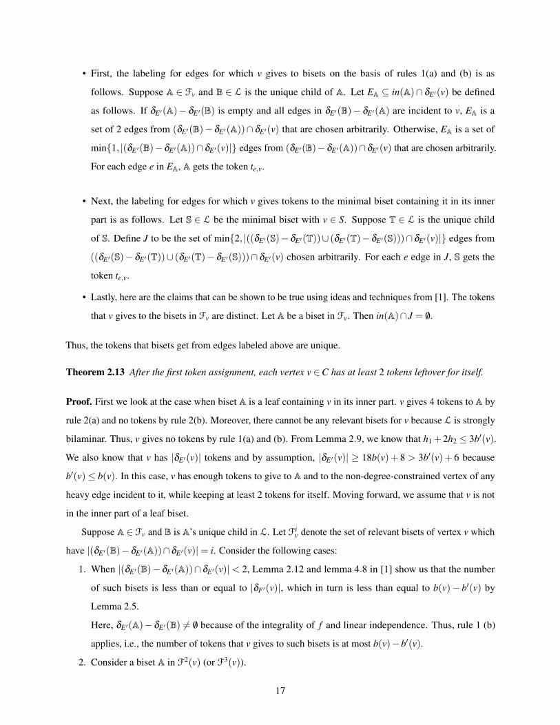
• First, the labeling for edges for which v gives to bisets on the basis of rules 1(a) and (b) is as

follows. Suppose A 2 Fv and B 2 L is the unique child of A. Let EA ✓ in(A)\ dE 0(v) be defined

as follows. If dE 0(A)� dE 0(B) is empty and all edges in dE 0(B)� dE 0(A) are incident to v, EA is a

set of 2 edges from (dE 0(B)� dE 0(A))\ dE 0(v) that are chosen arbitrarily. Otherwise, EA is a set of

min{1, |(dE 0(B)�dE 0(A))\dE 0(v)|} edges from (dE 0(B)�dE 0(A))\dE 0(v) that are chosen arbitrarily.

For each edge e in EA, A gets the token te,v.

• Next, the labeling for edges for which v gives tokens to the minimal biset containing it in its inner

part is as follows. Let S 2 L be the minimal biset with v 2 S. Suppose T 2 L is the unique child

of S. Define J to be the set of min{2, |((dE 0(S)�dE 0(T))[ (dE 0(T)�dE 0(S)))\dE 0(v)|} edges from

((dE 0(S)� dE 0(T))[ (dE 0(T)� dE 0(S)))\ dE 0(v) chosen arbitrarily. For each e edge in J, S gets the

token te,v.

• Lastly, here are the claims that can be shown to be true using ideas and techniques from [1]. The tokens

that v gives to the bisets in Fv are distinct. Let A be a biset in Fv. Then in(A)\ J = /0.

Thus, the tokens that bisets get from edges labeled above are unique.

Theorem 2.13 After the first token assignment, each vertex v 2C has at least 2 tokens leftover for itself.

Proof. First we look at the case when biset A is a leaf containing v in its inner part. v gives 4 tokens to A by

rule 2(a) and no tokens by rule 2(b). Moreover, there cannot be any relevant bisets for v because L is strongly

bilaminar. Thus, v gives no tokens by rule 1(a) and (b). From Lemma 2.9, we know that h1 +2h2 3b0(v).

We also know that v has |dE 0(v)| tokens and by assumption, |dE 0(v)| � 18b(v)+ 8 > 3b0(v)+ 6 because

b0(v) b(v). In this case, v has enough tokens to give to A and to the non-degree-constrained vertex of any

heavy edge incident to it, while keeping at least 2 tokens for itself. Moving forward, we assume that v is not

in the inner part of a leaf biset.

Suppose A 2 Fv and B is A’s unique child in L. Let Fiv denote the set of relevant bisets of vertex v which

have |(dE 0(B)�dE 0(A))\dE 0(v)|= i. Consider the following cases:

1. When |(dE 0(B)�dE 0(A))\dE 0(v)|< 2, Lemma 2.12 and lemma 4.8 in [1] show us that the number

of such bisets is less than or equal to |dF 0(v)|, which in turn is less than equal to b(v)� b0(v) by

Lemma 2.5.

Here, dE 0(A)�dE 0(B) 6= /0 because of the integrality of f and linear independence. Thus, rule 1 (b)

applies, i.e., the number of tokens that v gives to such bisets is at most b(v)�b0(v).

2. Consider a biset A in F2(v) (or F3(v)).

17

Here, one of the two (or three) edges in (dE 0(B)� dE 0(A))\ dE 0(v) must be a heavy edge due to

integrality of f , x(e) < 1 for every edge and linear independence. Thus, we can upper bound the

number of such bisets by the number of heavy edges. Hence,

|F2(v)|+ |F3(v))| 3b0(v).

Due to rule 1, v gives away at most 2 tokens to such bisets.

3. On the basis of rule 3 and Lemma 3.9, v might have to give away another 3b0(v) tokens.

4. Let A 2 F�4(v). We can conclude that F�4(v) |dE 0(v)|/4.

As a result of rule 1(a), v might have to give 2 tokens to every biset in F�4(v). Thus, the tokens that v

gives away here can be upper bounded by 2 |dE0 (v)|4 .

We want v to get 2 tokens, and the minimal biset containing v in its inner part (if such a biset exists) to get 2

tokens from v. Hence,

Number of tokens v needs (b(v)�b0(v))+3(3b0(v))+2|dE 0(v)|

4+4

= b(v)+8b0(v)+|dE 0(v)|

2+4

9b(v)+|dE 0(v)|

2+4

|dE 0(v)| (since |dE 0(v)|� 18b(v)+8 ) É

Remember that the final goal is to prove that the tokens can be rearranged so that each biset in L gets at least

two tokens, each vertex in C gets at least two tokens, and each maximal biset in L gets at least four tokens.

This would contradict |E|= |L|+ |C| from Theorem 2.7. This can be proved as follows.

Second token assignment: Each biset in L gets assigned some tokens in the initial token assignment and

the first token assignment. We show that we can rearrange these tokens so that each biset in L gets at least

two tokens and each maximal biset in L gets at least four tokens.

Proof. We consider each tree of L separately. Let T be a tree of L.

1. Consider a leaf A = (A,A0) of T. We have |dE 0(A)| � 2 because of the possibility of heavy edges.

Consider an edge e 2 dE 0(A) and let v be the endpoint of e that is in A. If v 2C, A gets at least 4 tokens.

However, it is possible that for every edge e 2 dE 0(A), the endpoint of e that is in A is not degree-

constrained. Such cases need to be examined closely, and we discuss them next.

(a) |dE 0(A)|= 2: Let e1 = (u1,v1) and e2 = (u2,v2) be the edges in dE 0(A), and v1,v2 2 A. Note that

v1,v2 /2C. It is not possible for both edges to be light because f (A)� 1 and it is integral.

18

i. e1 is light and e2 is heavy: A gets te1,v1 , te2,v2 and 1 token from u2 because u2 must be degree-

constrained by assumption, which means that rule 3 of the first token assignment applies.

Observe that u2 gives another token to v2 because of rule 3 in the first token assignment.

Thus, A receives a total of 4 tokens.

ii. e1 and e2 are both heavy: A gets te1,v1 , te2,v2 and a token from each of u1 and u2 because they

must be degree-bounded by assumption. Thus, A gets at least 4 tokens.

(b) |dE 0(A)|= 3: at least one edge crossing A has to be a heavy edge. Let this edge be e = (u,v) and

v 2 A. Remember that v /2C. We can see that A gets 2 tokens for e because u must be in C by

assumption and it gets te,v. In addition, it gets at least 2 tokens from the rest of the edges crossing

it. Hence, A gets a total of at least 4 tokens.

2. Next, we look at a non-leaf biset A. By induction, the tokens in each subtree that is rooted at a child of

A can be rearranged such that each biset in the subtree gets 2 tokens and the child biset gets 4 tokens.

Now, each child of A has 4 tokens and can give 2 of the 4 tokens to A. We can conclude that if A has

two or more children, then it gets at least 4 tokens. The more interesting case is when it has only child,

say B. Let E1 = dE 0(A)�dE 0(B) and E2 = dE 0(B)�dE 0(A). A gets 2 tokens from B. On the basis of

Lemma 2.11, one of the following must happen,

(a) |E1|� 2 and |E2|= 0:

Figure 2.4. Edges possible in E1.

Let e = (u,v) 2 E1 and v 2 A�B. Note that A is the minimal biset to contain v in its inner part.

If v 2C, A gets min{2, |E1\ dE 0(v)|} tokens from v by rule 2(b). In the case that e is a heavy

edge and v /2C, A gets 2 tokens because u must be in C by assumption; see rule 3 in first token

assignment. However if e is a light edge and v /2C, A gets te,v. Since there must be at least 2 such

edges, A gets at least 4 tokens in total.

19

(b) |E2|� 2 and |E1|= 0:

Figure 2.5. Edges possible in E2.

Note that E2 ✓ in(A) and for each edge e in E2, A is the minimal biset with e 2 in(A). If one of

the endpoints, say v, of such an edge e is in A�B and v 2C, A gets min{2, |E2\dE 0(v)|} tokens

from v (by first token assignment), i.e., a non-zero number of tokens. If v /2C, A gets te,v.

In the case that v is in bd(A)�B0 and v /2C, A gets the respective token. However, it is possible

that v 2C. Here, rule 1 of the first token assignment gives us 1 |EA| 2. Therefore, A still

gets at least 2 other tokens because |EA|� 2, making the total number of tokens at least 4.

(c) Both E1 and E2 are non-empty.

From the above two cases, we can see that A gets a token for each edge in E1 and E2. Since there

is at least 1 edge in both E1 and E2, A gets at least 2 tokens in addition to the 2 tokens that it gets

from B. Hence, A gets at least 4 tokens.

Finally, after reassigning the tokens, each vertex in C gets at least 2 tokens, each biset in L gets at least

2 tokens, and each maximal biset in L gets at least 4 tokens. This means that there must be more than

2(|L|+ |C|) number of tokens. This contradicts |L|+ |C|= |E|. É

20

Chapter 3

Degree-bounded rooted k-outconnectivity problem

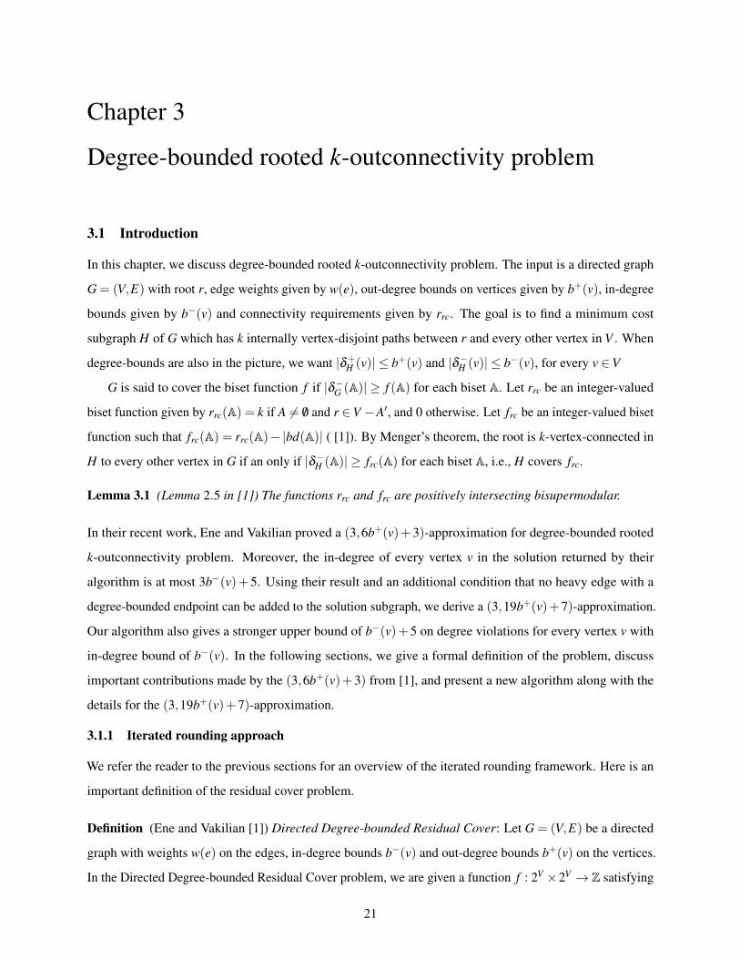
3.1 Introduction

In this chapter, we discuss degree-bounded rooted k-outconnectivity problem. The input is a directed graph

G = (V,E) with root r, edge weights given by w(e), out-degree bounds on vertices given by b+(v), in-degree

bounds given by b�(v) and connectivity requirements given by rrc. The goal is to find a minimum cost

subgraph H of G which has k internally vertex-disjoint paths between r and every other vertex in V . When

degree-bounds are also in the picture, we want |d+H (v)| b+(v) and |d�H (v)| b�(v), for every v 2V

G is said to cover the biset function f if |d�G (A)|� f (A) for each biset A. Let rrc be an integer-valued

biset function given by rrc(A) = k if A 6= /0 and r 2V �A0, and 0 otherwise. Let frc be an integer-valued biset

function such that frc(A) = rrc(A)� |bd(A)| ( [1]). By Menger’s theorem, the root is k-vertex-connected in

H to every other vertex in G if an only if |d�H (A)|� frc(A) for each biset A, i.e., H covers frc.

Lemma 3.1 (Lemma 2.5 in [1]) The functions rrc and frc are positively intersecting bisupermodular.

In their recent work, Ene and Vakilian proved a (3,6b+(v)+3)-approximation for degree-bounded rooted

k-outconnectivity problem. Moreover, the in-degree of every vertex v in the solution returned by their

algorithm is at most 3b�(v)+5. Using their result and an additional condition that no heavy edge with a

degree-bounded endpoint can be added to the solution subgraph, we derive a (3,19b+(v)+7)-approximation.

Our algorithm also gives a stronger upper bound of b�(v)+5 on degree violations for every vertex v with

in-degree bound of b�(v). In the following sections, we give a formal definition of the problem, discuss

important contributions made by the (3,6b+(v)+3) from [1], and present a new algorithm along with the

details for the (3,19b+(v)+7)-approximation.

3.1.1 Iterated rounding approach

We refer the reader to the previous sections for an overview of the iterated rounding framework. Here is an

important definition of the residual cover problem.

Definition (Ene and Vakilian [1]) Directed Degree-bounded Residual Cover: Let G = (V,E) be a directed

graph with weights w(e) on the edges, in-degree bounds b�(v) and out-degree bounds b+(v) on the vertices.

In the Directed Degree-bounded Residual Cover problem, we are given a function f : 2V ⇥2V ! Z satisfying

21

f (A) = r(A)� |bd(A)| for each biset A, where r is a biset function and the goal is to select a minimum

weight set F 0 ✓ E such that |d�F 0(A)|� f (A) for each biset A, and |d�F 0(v)| b�(v) and |d+F 0(v)| b+(v) for

each vertex v.

Ene and Vakilian in [1] give an iterated rounding algorithm for the Directed Degree-bounded Residual Cover

problem that achieves (O(1),O(1)b+(v))-approximation provided that the requirement function r satisfies

the following theorem.

Theorem 3.2 (Theorem 3.5 in [1]) Consider an instance of the Directed Degree-bounded Residual Cover

problem in which the function f satisfies f (A) = r(A)� |bd(A)|, where r is an integer-valued biset function.

Let OPT be the weight of an optimal soltuion for the instance. Suppose that r and f satisfy the following

conditions:

• For each biset (A,A0) and each vertex v 2 A0 �A, we have r((A,A0)) r((A,A0 � v)).

• The function f is positively intersecting bisupermodular.

Then there is a polynomial time iterated rounding algorithm that selects a set F 0 ✓ E of edges such that

w(F 0) 3OPT , |d�F 0(v)| 3b�(v)+5 and |d+F 0(v)| 6b+(v)+3 for each vertex v.

It is known that rrc satisifies the first condition and that frc is a positively intersecting bisupermodular biset

function (by Lemma 3.1). In [1], the previous theorem is applied with f = frc and r = rrc. This gives the

following result.

Theorem 3.3 (Theorem 3.6 in [1]) There is a polynomial time (3,6b+(v)+3)-approximation algorithm for

the Degree-bounded Rooted k-Outconnectivity problem in directed graphs. It also gives an upper bound of

3b�(v)+5 on the in-degree bounds given by b�(v).

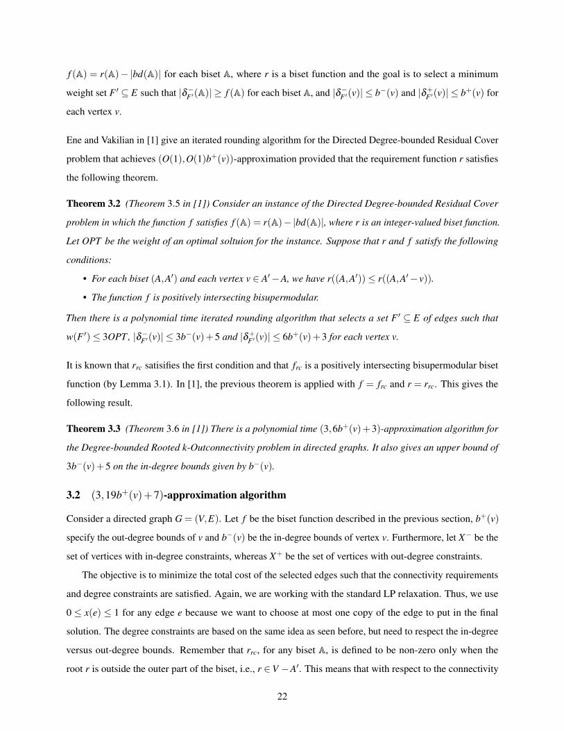
3.2 (3,19b+(v)+7)-approximation algorithm

Consider a directed graph G = (V,E). Let f be the biset function described in the previous section, b+(v)

specify the out-degree bounds of v and b�(v) be the in-degree bounds of vertex v. Furthermore, let X� be the

set of vertices with in-degree constraints, whereas X+ be the set of vertices with out-degree constraints.

The objective is to minimize the total cost of the selected edges such that the connectivity requirements

and degree constraints are satisfied. Again, we are working with the standard LP relaxation. Thus, we use

0 x(e) 1 for any edge e because we want to choose at most one copy of the edge to put in the final

solution. The degree constraints are based on the same idea as seen before, but need to respect the in-degree

versus out-degree bounds. Remember that rrc, for any biset A, is defined to be non-zero only when the

root r is outside the outer part of the biset, i.e., r 2V �A0. This means that with respect to the connectivity

22

requirements, we want some number of edges going into the biset. Hence, x(d�E (A))� f (A). The LP for

directed degree-bounded k-outconnectivity problem is as follows:

Directed-LP (Input:G = (V,E), f ,X�,X+,b�,b+)

min Âe2E

w(e)x(e)

s.t. x(d�E (A))� f (A) 8A : f (A)> 0

x(d�E (v)) b�(v) 8v 2 X�

x(d+E (v)) b+(v) 8v 2 X+

0 x(e) 1 8e 2 E

We propose an iterated rounding algorithm that works as follows: Each iteration of the while loop starts with

computing a basic optimal solution x to the LP. For notational convenience, we define an edge e to be heavy

in a basic feasible solution x if x(e)� 1/3. Otherwise, the edge is called a light edge. We refer to edges as

heavy or light throughout this thesis for notational convenience. Any iteration succeeds if either there is an

edge e with x(e) = 0 or 1, or there is a heavy edge which is not incident to any degree-bounded vertices, or

there is an in-degree bounded vertex with degree at most 5, or there is an out-degree bounded vertex with

degree at most 18b+(v)+7. Whenever an edge that is incident to a degree constrained vertex is added to the

solution, the corresponding bounds need to be updated so that the residual problem remains feasible. Our

main contribution is the following theorem.

Theorem 3.4 Consider an iteration of Directed-alg. Let G0 = (V,E 0) be the residual subgraph at the

beginning of this iteration. Let F 0 be the set of edges selected in the previous iterations. Let X� be the set

of vertices that have in-degree bounds, let p� : X� ! R be the in-degree bounds on X� at the beginning

of this iteration. Let X+ be the set of vertices that have out-degree bounds, let p+ : X+! R be the out-

degree bounds on X+ at the beginning of this iteration. Let f 0 : 2V ⇥ 2V ! Z be the function satisfying

f 0(A) = r(A)� |bd(A)|� |dF 0(A)| for each biset A. If x is a basic solution to Directed-LP for the input

(G0, f 0,X�,X+, p�, p+), one of the following holds:

• There exists an edge e 2 E 0 such that x(e) = 0.

• There exists e 2 E 0 such that x(e)� 1/3.

• There exists v 2 X� such that |d�E 0(v)| 5.

• There exists v 2 X+ such that |d+E 0(v)| 18b+(v)+7.

23

The algorithm is given below.

Directed-alg (Input:(G = (V,E),r,B�,B+,b�,b+)):

1. Let E 0 E,F 0 /0,X� B�,X+ B+

2. Let p�(v) b�(v) for each v 2 B� and p+(v) b+(v) for each v 2 B+

3. While E 0 is not empty

(a) Let f 0 : 2V ⇥2V : f 0(A) = r(A)� |bd(A)|� |dF 0(A)| for each A(b) Compute an optimal basic solution to LP with input (G0 = (V,E 0), f 0,X�,X+, p�, p+)

(c) If there is an edge e 2 E 0 such that x(e) = 0

• E 0 E 0 �{e}

(d) If there is an edge e 2 E 0 such that x(e) = 1

• F 0 F 0 [{e}

• E 0 E 0 �{e}

• If u 2 X+, p+ p+(u)�1

• If v 2 X�, p� p�(u)�1

(e) If there is an edge e = ~uv 2 E 0 such that x(e)� 1/3 and u /2 X+ and v /2 X�

• F 0 F 0 [{e}

• E 0 E 0 �{e}

(f) If there is a vertex v 2 X� such that |d�E 0(v)| 5

• X� X��{v}

(g) Else if there is a vertex v 2 X+ such that |d+E 0(v)| 18b+(v)+7

• X+ X+�{v}

4. Return F 0

Our proof of the above theorem is based on Ene and Vakilian’s approach in [1]. As a result of the above

theorem, we can say that since each edges that gets added has x(e)� 1/3, the weight of the solution is at

most 3OPT . Upper bounding the degree of vertices in the solution subgraph is all that remains to prove the

promised approximation bounds.

Lemma 3.5 Consider an iteration of Directed-alg. Let F 0 be the set of edges selected in the previous

iterations. Let X� be the set of vertices that have in-degree bounds, let p� : X� ! R be the in-degree bounds

on X� at the beginning of this iteration. Let X+ be the set of vertices that have out-degree bounds, let

p+ : X+! R be the out-degree bounds on X+ at the beginning of this iteration. For each vertex v 2 X�, we

24

have |d�F 0(v)| b�(v)� p�(v), where b�(v) is the initial in-degree bound on v. For each vertex in X+, we

have |d+F 0(v)| b+(v)� p+(v), where b+(v) is the initial out-degree bound on v.

We know that if the out-degree constraint on a vertex v was never dropped by the algorithm, |d+F 0(v)| b+(v).

However, if it does get dropped in some iteration, let F 00 represent the set of edges already selected by the

algorithm and E 00 be the set of remaining edges. Therefore, |d+F 0(v)| |d+

F 00(v)|+ |d+E 00(v)| 19b+(v)+ 7.

Using Theorem 3.4 and the previous lemma, we get the following theorem. Similarly for |d�F 0(v)| b�(v)+5.

As a result,

Theorem 3.6 Let F 0 be the solution constructed by Directed-alg. The set F 0 satisfies the following:

• |d�F 0(A)|� f (A) for each biset A.

• The total weight of F 0 is at most 3OPT .

• For each vertex v, we have |d�F 0(v)| b�(v)+5 and |d+F 0(v)| 19b+(v)+7.

3.3 Proof of Theorem 3.4

In this section, we give the proof for Theorem 3.4. We start with the following theorem that can be proved

using standard uncrossing technique ( [12]).

Theorem 3.7 (Nutov [12]) Let x be a basic solution to Directed-LP for an input (G=(V,E), f ,X�,X+,b�,b+).

If f is positively intersecting bisupermodular, there is a collection L of bisets and two sets C� ✓ X� and

C+ ✓ X+ of vertices with the following properties:

• 8A 2 L, x(d�E (A)) = f (A)> 0.

• 8v 2C�, x(d�E (v)) = b�(v).

• 8v 2C+, x(d+E (v)) = b+(v).

• The family L is bilaminar.

• |L|+ |C�|+ |C+|= |E|.

• The vectors in {c(d�E (A)) | A 2 L}[{c(d�E (v)) | v 2C� }[{c(d+E (v)) | v 2C+ } are linearly inde-

pendent.

As seen in Lemma 3.1, f is positively intersecting bisupermodular. From Lemma 1.2, we know that d�F (.)

is bisubmodular. As a result, f 0 is also positively intersecting bisupermodular. Thus, Theorem 3.7 can be

applied to x and (G0 = (V,E 0), f 0,X�,X+, p�, p+) to get a collection L of tight bisets and sets C� and C+ of

tight vertices.

We prove Theorem 3.4 by contradiction. This means that all of the following is assumed to hold:

• For every edge e, 0 < x(e)< 1.

25

• For any edge e, either x(e)� 1/3 and u 2 X+ or v 2 X�, or x(e)< 1/3.

• For every in-degree constrained vertex v 2 X�, |d�E 0(v)|� 6.

• For every out-degree constrained vertex v 2 X+, |d+E 0(v)|� 18b+(v)+8.

In the token argument, we assign two tokens for each edge in E 0, making the total number of tokens equal

to 2|E 0|. The goal here is to prove that these tokens can be distributed so that each biset in L gets at least

two tokens, each vertex in C� and C+ gets at least two tokens, and each maximal biset in L gets at least four

tokens. This would contradict the condition |E|= |L|+ |C+|+ |C�| from Theorem 3.7. Here again, we view

L as a rooted forest based on biset-inclusion relation.

Here is an important definition about relevance of a biset for a vertex v and a property that such relevant

bisets satisfy. We care about the relevant bisets of degree-constrained vertices because they affect the token

assignment scheme.

Definition (Ene and Vakilian [1]) A bisetA2L is relevant for a vertex v2V if all of the following conditions

hold:

• A has one child.

• The vertex v is on the boundary of A but not on the boundary of the child of A.

Lemma 3.8 (Lemma 4.8 in [1]) Let v be a vertex in V . If L is a bilaminar family, the relevant bisets of v are

pairwise disjoint.

We use a token assignment that is similar to the one from [1]. Any changes are marked with (⇤). Let

din(A) := {~uv|u 2 A0,v 2 A}, i.e., edges in A pointing towards A. Token assignment happens in multiple

stages, which is described via the following token assignments.

Initial token assignment: ( [1]) Each edge ~uv 2 E 0 has two tokens te,u and te,v, one for each endpoint. The

edge e distributes its tokens to L[C�[C+ as follows:

• (Rule A) If u 2C+, the token te,u goes to u.

• (Rule B) If v 2C�, the token te,v goes to v.

• (Rule C) If u /2C+ and 9A 2 L such that ~uv 2 din(A), the token te,u is assigned to the minimal such

biset A. Otherwise, the token is unsassigned.

• (Rule D) If v /2C� and 9A 2 L such that e 2 d�E 0(A), the token te,v is assigned to the minimal such

biset A. Otherwise, the token is unassigned.

Thus, each token is assigned to at most one member of L[C�[C+. The tokens are reassigned in two stages.

By the definition of relevant bisets and lemma 1.4, we can see that the relevant bisets of a degree-bounded

vertex are pairwise disjoint.

26

First token assignment:

1. Each vertex v 2C� receives |d�E 0(v)| tokens in the initial token assignment. For each vertex v 2C�, if

there exists a biset A with v 2 A such that d�E 0(A)\d�E 0(v) 6= /0, v gives 4 tokens to such a minimal biset

A.

2. Each vertex u 2C+ receives |d+E 0(u)| tokens in the initial token assignment.

(a) Consider a relevant biset for u, and call it A.

i. If d�E 0(A)�d�E 0(B) is empty and all edges in d�E 0(B)�d�E 0(A) are outgoing edges of u, u gives

2 tokens to A.

ii. Otherwise, u gives min{1, |(d�E 0(B)�d�E 0(A))\d+E 0(u)|} to A.

(b) Suppose A is the minimal biset that contains u in its inner part.

i. (⇤) If A is a leaf, it gets 2 tokens from u.

ii. If A has unique child B, then u gives min{2, |(d�E 0(B)�d�E 0(A))\d+E 0(u)|} tokens to A.

3. (⇤) For a vertex u 2C+, if there is a heavy edge e in d+E 0(u) such that the other endpoint, say v, is not in

C�, then u gives a token to v (based on [2]). If such a v is in a leaf biset A and x(e)� 2/3, then u gives

a token to A.

We refer the reader to the previous discussion (in section 2.3) for why we use these rules for first token

assignment. Following is a lemma that bounds the number of tokens that any degree-constrained vertex might

have to give to bisets or the other endpoint of edges incident to it.

Lemma 3.9 Let u 2C+, h1 be the number of heavy edges e1 2 d+E 0(v) with 1/3 x(e1)< 2/3 and h2 be the

number of edges in e1 2 d+E 0(v) with 2/3 x(e2)< 1. Then h1 +h2 3p+(v).

Proof. We know that x(d+E (v)) b+(v). Let h1 be the number of heavy edges e1 2 d+

E 0(v) with 1/3 x(e1)<

2/3 and h2 be the number of edges in e1 2 d+E 0(v) with 2/3 x(e2) < 1. Thus, p+(v) � 1

3 h1 +23 h2 =)

3p+(v)� h1 +2h2. É

Corollary 3.10 There can be at most 3p+(u) heavy edges going out of vertex u 2C+, and at most 3p�(v)

heavy edges going into vertex v 2C�.

Next, we see an important lemma that we will need in the case analysis. It follows from the fact that the

characteristic vectors of bisets in L must be linearly independent, f 0 must be integer-valued and that there

might be heavy edges incident to degree-bounded vertices that cannot be added to the solution.

Lemma 3.11 Let A be a biset that has a unique child B in L. Then one of the following holds:

• d�E 0(A)�d�E 0(B) has at least 2 edges.

27

• d�E 0(B)�d�E 0(A) has at least 2 edges.

• d�E 0(A)�d�E 0(B) and d�E 0(B)�d�E 0(A) are both non-empty.

Here is an important lemma that relies on Theorem 3.2, and is needed in the main proof (as seen later).

Lemma 3.12 (Lemma 6.10 in [1]) Let u be a vertex and let A= (A,A0) be a tight biset with u on its boundary.

If d+F 0(u)\din(A) is empty, |d+

E 0(u)\din(A)|� 2.

A really important step in the main proof is to show that each degree-bounded vertex has enough tokens for

itself and any bisets or vertices that might require tokens from it. To do so, we borrow the following from [1].

Let Fu be the set of all relevant bisets of u. By lemma 1.4, the bisets in Fu are pairwise disjoint. Thus, sets in

{din(A\d+E 0(u))|A 2 Fu} are pairwise disjoint.

• The tokens that u gives to bisets on the basis of rule 2 can be labeled as follows. Suppose A 2 Fu

and let B be its unique child in L. Let EA ✓ din(A)\d+E 0(u) be defined as follows. If d�E 0(A)�d�E 0(B)

is empty and all edges in d�E 0(B)� d�E 0(A) are outgoing edges of u, EA is the set of 2 edges from

(d�E 0(B)� d�E 0(A))\ d+E 0(u) that are chosen arbitrarily. Otherwise, it is a set of min{1, |(d�E 0(B)�

d�E 0(A))\d+E 0(u)|} edges from (d�E 0(B)�d�E 0(A))\d+

E 0(u) that are chosen arbitrarily. For each edge e

in EA, A gets the token te,u.

• The labeling for edges for which u gives tokens to the minimal biset containing v in its inner part is

as follows. Let S 2 L be the minimal biset with u 2 S and T be its unique child in L. Let J be a set

of min{2, |(d�E 0(B)�d�E 0(A))\d+E 0(u)|} edges of (d�E 0(B)�d�E 0(A))\d+

E 0(u) that are chosen arbitrarily.

For each edge e in J, S gets te,u from u.

• Lastly, here are the statements that can be shown to be true using methods in [1]. The tokens given by

u to the bisets in Fu are distinct. Let A 2 Fu. Then din(A)\ J = /0.

Thus, the tokens that bisets get from edges labeled as described above are unique.

Theorem 3.13 After the first token assignment, each degree-bounded vertex has at least 2 tokens for itself.

Proof. For every v 2C�, |d�E 0(v)| � 6 and v gives away at most 4 tokens (by Rule 1 from the first token

assignment). Thus, such a v has at least 2 tokens leftover for itself.

Next, we look at vertices u 2C+. Let us first examine the case when u is contained in the inner part of

a leaf biset A. Due to L being a bilaminar family of bisets, we know that there can only be one such biset.

By assumption, |d+E 0(v)|� 18b+(v)+8. On the basis of rule 2 (b), we know that u gives 2 tokens to A. In

28

addition, Lemma 3.9 shows that h1 +h2 3p+(u), so u needs at most 3p+(u) tokens for vertices that must

get tokens by rule 3. Lastly, u also needs 2 tokens for itself. It is evident that u collects enough tokens from

the incident edges (with u as the tail) to have plenty tokens for any bisets, vertices and itself.

Now consider the case when A 2 Fu and B is its unique child in L. Also, u 2C+. Let Fiu denote the set

of relevant bisets of vertex u with |(d�E 0(B)�d�E 0(A))\d+E 0(u)|= i. Consider the following cases:

1. When |(d�E 0(B)�d�E 0(A))\d+E 0(u)|< 2, Lemma 3.12 and lemma 1.4 suggest that the number of such

bisets must be less than or equal to |d+F 0(u)|, which in turn is less than or equal to b+(v)� p+(v) by

Lemma 3.5.

Here, d�E 0(A)�d�E 0(B) 6= /0 because of the integrality of f and linear independence. Thus, rule 1 (b)

applies, i.e., u gives at most b+(v)� p+(v) tokens to such bisets.

2. Next we look at bisets in F2(u) (or F3(u)).

At least one edge in (d�E 0(B)�d�E 0(A))\d+E 0(u) must be a heavy edge because f is an integral values

biset function. Therefore, we can upper bound the number of these bisets by the number of heavy

edges. Hence,

|F2(u)|+ |F3(u)| 3p+(u).

As a result of rule 1, v gives at most 2 tokens to such bisets.

3. On the basis of rule 3 and Lemma 3.9, u might have to give away another 3p+(u) tokens.

4. Let A 2 F�4(u), so F�4(u) |d+E 0(u)/4|.

On the basis of rule 1 (a), u might have to give up 2 tokens to every biset in F�4(u). Thus, the tokens

that u gives up can be upper bounded by 2|d+

E0 (u)|4 .

In addition, we want u to get 2 tokens, and the minimal biset containing u in its inner part (if such a biset

exists) to get 2 tokens from v. Hence,

Number of tokens u needs (b+(u)� p+(u))+3(3p+(u))+2|d+

E 0(u)|4

+4

= b+(u)+8p+(u)+|d+

E 0(u)|2

+4

9b+(u)+|d+

E 0(u)|2

+4

|d+E 0(u)| (since |d+

E 0(u)|� 18b+(u)+8 ) É

Now that we have discussed all the different pieces needed to finish the main proof, let us move onto the last

token (re)assignment step.

29

Second token assignment: Each biset in L gets assigned some tokens in the initial token assignment and

the first token assignment. These tokens can be reassigned such that each biset in L gets at least two tokens

and each maximal biset in L gets at least four tokens.

Proof. We look at each tree, T, in L separately.

1. Consider a leaf A= (A,A0) of T. We know that |d�E 0(A)|� 2 because of the possibility of heavy edges.

Let e 2 d�E 0(A) and v be the endpoint of e that is in A, i.e., the inner part of A. If v 2C�, then A gets 4

tokens from v by rule 1 of the first token assignment. Otherwise, it gets te,v.

We need to closely examine the case when |d�E 0(A)| is either 2 or 3, and A does not own any degree-

constrained vertices.

(a) |d�E 0(A)|= 2: Let e1 = ~u1v1 and e2 = ~u2v2 be the two edges in d�E 0(A), and v1,v2 2 A. Note that

v1,v2 /2C�. It is not possible for both edges to be light because f (A)� 1 and it is integral.

i. Suppose e1 is light and e2 is heavy. A gets te1,v1 , te2,v2 and te2,u2 (by rule 3(⇤)). In addition,

u2 gives another token to A by rule 3(⇤). Thus, A gets 4 tokens.

ii. e1 and e2 are both heavy: A gets te1,v1 , te2,v2 and a token from each of u1 and u2 because they

must be degree-bounded by assumption. Thus, A gets at least 4 tokens.

(b) |d�E 0(A)| = 3: one of the three edges in d�E 0(A) has to be a heavy edge because f is an integer-

valued biset function. Let this edge be e = ~uv. Remember that v /2C�. Here again, by rule 3(⇤),

A gets both tokens for e. It can also get at least 1 token from each of the other edges in d�E 0(A).Therefore, A gets at least 4 tokens.

2. Now we look at the cases when A is not a leaf biset. By induction, the tokens in each subtree rooted at

a child of A can be reassigned such that each biset in the subtree gets 2 tokens and the child biset gets

4 tokens. We can see that each child needs 2 tokens for itself and can therefore give 2 tokens to A. This

means that when A has at least 2 children, it can get at least 4 tokens for itself. At the same time, every

biset in the subtree gets 2 tokens each. The case that needs a closer examination is when A has only

one child, say B. Let E1 = d�E 0(A)�d�E 0(B) and E2 = d�E 0(B)�d�E 0(A). On the basis of Lemma 3.11,

one of the following must happen,

(a) |E1|� 2 and |E2|= 0:

Let ~uv 2 E1 and v 2 A�B, which makes A the minimal biset containing v. If v 2C�, then A gets

4 tokens from v by rule 1. In the case that v /2C�, A gets te,v. Thus, it can get at least one token

per edge in E1, and 2 tokens from the child biset B. This makes the total number of tokens at

least 4.

(b) |E2|� 2 and |E1|= 0:

30

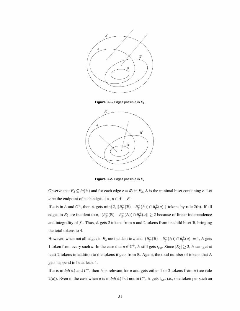
Figure 3.1. Edges possible in E1.

Figure 3.2. Edges possible in E2.

Observe that E2 ✓ in(A) and for each edge e = ~uv in E2, A is the minimal biset containing e. Let

u be the endpoint of such edges, i.e., u 2 A0 �B0.

If u is in A and C+, then A gets min{2, |(d�E 0(B)�d�E 0(A))\d+E 0(u)|} tokens by rule 2(b). If all

edges in E2 are incident to u, |(d�E 0(B)�d�E 0(A))\d+E 0(u)| � 2 because of linear independence

and integrality of f 0. Thus, A gets 2 tokens from u and 2 tokens from its child biset B, bringing

the total tokens to 4.

However, when not all edges in E2 are incident to u and |(d�E 0(B)�d�E 0(A))\d+E 0(u)|= 1, A gets

1 token from every such u. In the case that u /2C+, A still gets te,u. Since |E2|� 2, A can get at

least 2 tokens in addition to the tokens it gets from B. Again, the total number of tokens that Agets happend to be at least 4.

If u is in bd(A) and C+, then A is relevant for u and gets either 1 or 2 tokens from u (see rule

2(a)). Even in the case when u is in bd(A) but not in C+, A gets te,u, i.e., one token per such an

31

edge e. |E2|� 2 implies that A can still collect at least 4 tokens in total, 2 of which come from B.

(c) Both E1 and E2 are non-empty:

From the above two cases, we can conclude that A will get at least one token for every edge in E1

and E2, each of which contains at least an edge. Moreover, A gets 2 tokens from B. Hence, Areceives a total of at least 4 tokens.

In conclusion, after reassigning the tokens, each vertex in C+[C� has at least 2 tokens, each biset in L

has at least 2 tokens, and each maximal biset in L has at least 4 tokens. Assuming L is non-empty, the number

of tokens is strictly greater than 2|L|+2|C+|+2|C�|= 2|E 0| and this is enough to get a contradiction. É

32

Chapter 4

Conclusions

We presented approximation algorithms for two NP-Hard problems, namely degree-bounded Elem-SNDP

and degree-bounded rooted k-outconnectivity problem. Our goal was to develop a better understanding of

the known machinery for such problems in order to explore the possibility of a new algorithm or simpler

proof idea. In the process of proving the results discussed in the previous chapters, we also looked into

other reasonable approximation bounds. Some questions we wanted answered were: Can the constants be

improved upon? Can we prove an (O(1),O(1)b(v)+O(rmax))-approximation for algorithm for Elem-SNDP,

or an (O(1),O(1)b+(v)+O(rmax))-approximation for our algorithm for rooted k-outconnectivity problem?

Can we make things work without leaning on the idea of corequirement? Specifically for EC-SNDP, we

also studied the possibility of extending the proof technique from [15] to the degree-bounded setting. In this

chapter, we discuss our findings for these questions.

On the basis of the discussion so far, it is clear that we have an (O(1),O(1)b(v))-approximation for

Elem-SNDP and (O(1),O(1)b+(v))-approximation for rooted k-outconnectivity problem. However, the

actual constants are not comparable to what is already known. This motivated us to investigate if techniques

from [1] could be modified to get any improvements. In [1], we knew that the number of edges crossing

any biset had to be at least 4 and this played a key role in the proofs. But for our approach, the existence

of heavy edges that cannot be added to the solution is undeniable. As a result, we can only promise that

there must be at least 2 edges crossing each biset. This in turn prevents proofs motivated by [1] from going

through. In addition, smaller constants make it hard to account for the number of tokens a degree constrained

vertex needs to give to its relevant bisets in the token counting argument. Another thing to notice is that for

the inductive proof of the main theorems in [1], leaves received at least 4 tokens each. This was crucial for

making sure that the inductive argument would go through. Showing that a leaf gets enough tokens relied

on there being at 4 edges crossing the leaf, which we know is not true for us. As a result, we made a few

changes to the token assignment scheme so that it still followed the same idea.

We know that in the context of EC-SNDP, Lau and Zhou in [2] were able to unify the known techniques

to get a simplified algorithm. This suggested that a min{O(1)b(v),O(1)b(v)+O(rmax)}-approximation for

the degree violations, with small constants, could be an avenue worth pursuing. Remember that we need

bisets for Elem-SNDP and rooted k-connectivity problem. Thus, this would involve translating the ideas for a

33

laminar family of sets to a bilaminar family of bisets. As long as a degree constrained vertex is in the inner

part of a biset, similar ideas can be applied. What about the case when such a vertex was in the boundary of

a biset? Does it still make sense to ensure that as long as b(v) � 6rmax, the proof would go through? The

problem lies in the token counting argument, where we need to show that a degree constrained vertex has

enough tokens for itself and any bisets or vertices that need tokens from it. This technique as a whole is even

more unclear for directed graphs.

Can Fukunaga et al.’s algorithm and techniques in [14] be extended for our algorithm instead? They gave

an important structural lemma that upper bounds the number of bisets that can have a vertex in their boundary.

Lemma 4.14 (Lemma 4.5 in [14]) Let L be a biset family on V , let C ✓V , let E be the set of leaves of L, let

g = maxA2L

|bd(A)|, and let �L(v) be the number of bisets in L with v in their boundary. Then

Âv2C

max{�L(v),1} 2g(|E|�1)+ |C| if L is laminar

Âv2C

max{�L(v),1} g|E|+ |C| if L is strongly laminar

This proves useful in analyzing the case when |C| is greater than |E| or a multiple of it. However, it is unclear

if the other case can work for an (O(1)b(v)+O(rmax))-approximation on the degree violations. As we can

see, accounting for the number of tokens that a degree-contrained vertex needs to give to bisets and/or other

endpoints of heavy edges incident to them is a recurring bottleneck.

Other than the two problems discussed in this thesis, we also tried extending an alternate proof (from [15])

to Jain’s iterative rounding algorithm for EC-SNDP to the setting with degree bounds. It is an inductive

argument that relies on showing that if we start out with 1 token per edge, then we can prove that |L|> |C|

which would contradict the rank lemma for the corresponding LP. Using a proof by induction, Chekuri and

Rukkanchanunt first give a relation between the maximal sets, respective requirement functions and the

number of edges crossing the maximal sets in the laminar family. Next, they count the number of endpoints

(or tokens) that each set owns, which turn out to be more than |E 0|; E 0 is the set of edges crossing the maximal

sets. As in any other proof, this also involved case analysis in order to prove the recursive claim. This

considerably simplified the proof and could be viewed as more intuitive. A natural question here was to check

if this technique could be used to prove the known (2,2b(v)+3)- or (2,2b(v)+2)-approximation. However,

the claim is not strong enough to capture the imbalance in the way tokens from a heavy edge get assigned;

see [7] and [9] for details. Another issue is that there does not seem to be a direct, or clean, relation between

b(v) and the number of incident edges. It would be interesting to have this technique looked into and get a

better understanding of whether it even extends to the degree-bounded setting.

34

References

[1] A. Ene and A. Vakilian, “Improved approximation algorithms for degree-bounded networkdesign problems with node connectivity requirements,” Proceedings of the 46th AnnualACM Symposium on Theory of Computing - STOC ’14, 2014. [Online]. Available: http://cs-people.bu.edu/aene/papers/deg-bd-stoc.pdf

[2] L. C. Lau and H. Zhou, “A unified algorithm for degree bounded survivable network design,” Mathe-matical Programming, vol. 154, no. 1-2, p. 515–532, 2015.

[3] R. M. Karp, “Reducibility among combinatorial problems,” Complexity of Computer Computations, p.85–103, 1972.

[4] M. Singh and L. C. Lau, “Approximating minimum bounded degree spanning trees to withinone of optimal,” Journal of the ACM, vol. 62, no. 1, p. 1–19, Feb 2015. [Online]. Available:https://cs.uwaterloo.ca/~lapchi/papers/mbdst.pdf

[5] A. Gupta and J. Könemann, “Approximation algorithms for network design: A survey,” p. 1–16.[Online]. Available: http://www.cs.cmu.edu/~anupamg/papers/network-survey.pdf

[6] K. Jain, “A factor 2 approximation algorithm for the generalized steiner network problem,” Combinator-ica, vol. 21, no. 1, p. 39–60, Jan 2001.

[7] L. C. Lau, J. S. Naor, M. R. Salavatipour, and M. Singh, “Survivable network design with degree ororder constraints,” SIAM Journal on Computing, vol. 39, no. 3, p. 1062–1087, 2009.

[8] L. C. Lau and M. Singh, “Additive approximation for bounded degree survivable network design,”SIAM J. Comput. SIAM Journal on Computing, vol. 42, no. 6, p. 2217–2242, 2013. [Online]. Available:https://cs.uwaterloo.ca/~lapchi/papers/additive.pdf

[9] A. Louis and N. K. Vishnoi, “Improved algorithm for degree bounded survivable network designproblem,” Lecture Notes in Computer Science Algorithm Theory - SWAT 2010, p. 408–419, 2010.[Online]. Available: http://arxiv.org/pdf/0911.4544v1.pdf

[10] L. Fleischer, K. Jain, and D. P. Williamson, “Iterative rounding 2-approximation algorithms forminimum-cost vertex connectivity problems,” Journal of Computer and System Sciences, vol. 72, no. 5,p. 838–867, 2006. [Online]. Available: https://people.orie.cornell.edu/dpw/papers/elcon2.ps

[11] L. C. Lau, R. Ravi, and M. Singh, Iterative methods in combinatorial optimization. Cambridgeuniversity press, 2011.

[12] Z. Nutov, “Degree constrained node-connectivity problems,” Algorithmica, vol. 70, no. 2, p. 340–364,2013. [Online]. Available: http://www.openu.ac.il/home/nutov/deg-ncon.pdf

35

[13] T. Fukunaga and R. Ravi, “Iterative rounding approximation algorithms for degree-bounded node-connectivity network design,” 2012 IEEE 53rd Annual Symposium on Foundations of Computer Science,2012.

[14] T. Fukunaga, Z. Nutov, and R. Ravi, “Iterative rounding approximation algorithms for degree-boundednode-connectivity network design,” SIAM J. Comput. SIAM Journal on Computing, vol. 44, no. 5, p.1202–1229, 2015. [Online]. Available: http://epubs.siam.org/doi/pdf/10.1137/13094503x

[15] C. Chekuri and T. Rukkanchanunt, “A note on the survivable network design problem,” 2016. [Online].Available: https://arxiv.org/abs/1608.02515

36