Embed Size (px)
Citation preview

c© 2014 Logan Niehaus
ROBOTS AS LANGUAGE USERS:A COMPUTATIONAL MODEL FOR PRAGMATIC WORD LEARNING
BY
LOGAN NIEHAUS
DISSERTATION
Submitted in partial fulfillment of the requirementsfor the degree of Doctor of Philosophy in Electrical and Computer Engineering
in the Graduate College of theUniversity of Illinois at Urbana-Champaign, 2014
Urbana, Illinois
Doctoral Committee:
Professor Stephen E. Levinson, ChairProfessor Thomas HuangProfessor Mark Hasegawa-JohnsonProfessor David Vernon, University of SkovdeProfessor Giorgio Metta, Istituto Italiano di Tecnologia
ABSTRACT
The development of machines capable of natural linguistic interaction with
humans has been an active and diverse area of research for decades. More
recent frameworks, such as Cognitive Robotics, have been able to make
progress on many long-standing problems in computational modeling of lan-
guage acquisition – like that of symbol grounding – through the application
of the principles of embodied cognition. Many of these systems have focused
on modeling grounded word learning through statistical mappings between
various sensor modalities, such as speech-to-vision or speech-to-motor con-
trol. However, the entire body of such systems has only been able to capture
a tiny fraction of the developmental robustness or representational diversity
observed in even the youngest of human word-learners. Children are capable
of learning words in situations of extreme ambiguity, leveraging a variety of
contextual knowledge to infer the targets of adults’ references. And unlike
children, few cognitive robotics systems have any kind of understanding of
the purpose of words outside of reference. The core premise of the following
thesis is that this gap is, in part, due to computational models which ignore
the communicative and intentional (i.e. pragmatic) aspects of language.
To address these issues, a computational framework for the learning of
perceptually-grounded word meanings is presented. Our model is based on
a representation of language as a useful behavior, embedded within an inten-
tionally structured social interaction. Using techniques for inverse planning
and control, the algorithms we have developed seek to understand the goal
or purpose driving the behaviors of the interaction. We describe the appli-
cation of these techniques to a set of human-robot interaction experiments,
modeled after development studies demonstrating specific skills of children
in the learning of word meanings under referential ambiguity. Through these
experiments, we show how our framework allows the robotic agent to acquire
knowledge about the physical and social task structure underlying the inter-
action, and leverage this in order to learn word meanings in many different
cases of ambiguity. These include many novel situations where the robot
ii

must make inferences due to the goal-directed actions of the speaker, or
even knowledge of its own embodiment and potential role in the interaction.
We will show finally how our robotic platform can be made to realize this
role, actively taking part in its own learning experience, and begin to see
language as something useful.
iii
TABLE OF CONTENTS
CHAPTER 1 INTRODUCTION . . . . . . . . . . . . . . . . . . . . 11.1 Current Issues with Early Language Acquisition Models . . . 31.2 Bridging the Gap . . . . . . . . . . . . . . . . . . . . . . . . . 51.3 Purpose and Contribution of This Thesis . . . . . . . . . . . 71.4 Thesis Organization . . . . . . . . . . . . . . . . . . . . . . . 8
CHAPTER 2 REVIEW OF RELATED RESEARCH . . . . . . . . . 102.1 Embodied Systems for Linguistic Interaction . . . . . . . . . 102.2 Pragmatic Models of Language Acquisition . . . . . . . . . . 162.3 Mathematical Tools for Cognitive Modeling . . . . . . . . . . 21
CHAPTER 3 A PRAGMATIC MODEL FOR EARLY WORDLEARNING . . . . . . . . . . . . . . . . . . . . . . . . . . . . . . . 413.1 Overview and Motivation . . . . . . . . . . . . . . . . . . . . 413.2 Basic Pragmatic Model . . . . . . . . . . . . . . . . . . . . . 463.3 Extended Pragmatic Model . . . . . . . . . . . . . . . . . . . 523.4 Triadic Pragmatic Model . . . . . . . . . . . . . . . . . . . . 63
CHAPTER 4 GROUNDING LANGUAGE IN PERCEPTUALREPRESENTATIONS . . . . . . . . . . . . . . . . . . . . . . . . . 714.1 Perceptual Simulators . . . . . . . . . . . . . . . . . . . . . . 714.2 Learning of Speech and Action Representations . . . . . . . . 73
CHAPTER 5 ROBOT IMPLEMENTATION . . . . . . . . . . . . . 805.1 The iCub Humanoid Robot . . . . . . . . . . . . . . . . . . . 805.2 Application of the Pragmatic Model . . . . . . . . . . . . . . 815.3 Visual Processing . . . . . . . . . . . . . . . . . . . . . . . . . 86
CHAPTER 6 HUMAN-ROBOT INTERACTION EXPERIMENTS . 966.1 Experiment I: Pragmatic Learning of Basic Object-Words . . 966.2 Experiment II: Learning from Intentional Behavior . . . . . . 1056.3 Experiment III: Learning from Social Interaction . . . . . . . 1166.4 General Discussion . . . . . . . . . . . . . . . . . . . . . . . . 125
CHAPTER 7 CONCLUSION . . . . . . . . . . . . . . . . . . . . . . 1307.1 Future Work . . . . . . . . . . . . . . . . . . . . . . . . . . . 1327.2 Final Remarks . . . . . . . . . . . . . . . . . . . . . . . . . . 133
REFERENCES . . . . . . . . . . . . . . . . . . . . . . . . . . . . . . . 134
iv
CHAPTER 1
INTRODUCTION
The development of systems through which computers and other artificial
agents are able to use language in the way humans do has been an active
area of study for many decades. Early work focused on the recognition of
human speech through the application of statistical methods and models,
trained on large corpora of expertly annotated speech data. While automatic
speech recognition (ASR) systems have seen incremental and steady progress
over the years, most still remain inherently limited in their capabilities.
Beyond lingering issues of robustness to noise, speaker variations, and poor
accuracy for general word recognition tasks, ASR systems largely capture
only the phonological and syntactic aspects of natural language. These
systems for the most part have no understanding of the meaning of what is
being said, or purpose of what is being said; i.e. the semantic and pragmatic
aspects of language. Without these components, realistic linguistic use and
ultimately linguistic interaction between humans and machines remains out
of reach. Historically, extensions to basic ASR systems have attempted to
integrate these aspects through a similar paradigm: rudimentary symbolic
representations of meaning or dialog, constructed by human experts, are
attached to the text strings translated from speech data. These approaches
have proved as brittle and limited in capability as the symbol-manipulation
systems upon which they were based.
One proposed explanation for the limitations of this paradigm comes from
the embodied cognition hypothesis, which states that human cognition (and
cognition in general) is a product of the functional and developmental pro-
cesses of its physical embodiment. This embodiment includes not only the
parts of the brain associated with high-level cognition of the type used by
symbol-manipulation systems, but also those structures supporting sensory
and motor capabilities. Furthermore, this embodiment is situated within a
physical environment with which it is constantly interacting. Perception,
action, and cognition are all part of a continuous, interconnected cycle that
develops in real-time. Under this view, linguistic representations must be
1
embedded within this cycle, and are subject to the constraints, both physi-
cal and developmental, that are imposed by the agent’s embodiment. Items
such as linguistic symbols are no longer preordained by the system designer
and independent of the agent’s embodiment, but rather are grounded in
perceptual representations specific to the agent’s sensorimotor abilities, and
are formed continuously, as the agent interacts with and experiences its
environment.
For artificial agents, this requirement of sensorimotor experience is often
made achievable through the use of a robotic platform. The field of cog-
nitive developmental robotics (CDR) is one such area in which principles
and ideas of embodied cognitive development are applied to the construc-
tion of computational methods for artificial agents [1, 2, 3]. CDR generally
values methods that are centered around biologically and developmentally
feasible algorithms for learning and adaptation, rather than the traditional
approach of expert-guided training of complex models using large corpora
of data. With respect to language, approaches in this area have focused on
sensorimotor integration and processes for acquiring the core components of
the linguistic faculty: speech, syntax, and semantics. The rich set of sen-
sorimotor information afforded by many robotic platforms has allowed for
striking improvements at the level of semantics in particular.
On this specific topic, CDR has already proven its usefulness in grounded
word learning. The challenges of grounded word learning include issues of
both the structure of perceptual (sensorimotor) and conceptual (semantic)
representations, and how these two components come to interact. Research
over the past decade has produced robotic systems which are able to learn
the meanings of words for objects [4, 5, 6], events [7], and actions [8, 9, 10]
from real sensorimotor data, often in ways that capture aspects of the sta-
tistical processing capabilities seen in humans. Some of these systems are
even capable of exploiting acquired linguistic knowledge to further their per-
ceptual, cognitive, or interactive capabilities in ways that are far beyond the
scope of traditional speech and language processing systems. However, when
compared with the abilities of human language learners, these achievements
appear to cover only limited portions of a human’s general word-learning
competence, and do so in a piecemeal fashion. Most systems focus on learn-
ing words of a single type or category, and almost no progress has been made
in representing how a word’s use is tied to its meaning. In addition, learning
algorithms are driven primarily by statistical processing power, or a number
of various domain-specific heuristics used to mitigate perceptual confusion.
There has been little work in the direction of developing frameworks that
2
can more easily generalize across word categories or learning principles, and
that will allow robots to interact linguistically with humans at a level that
comes anywhere near even the most basic language users.
1.1 Current Issues with Early Language AcquisitionModels
Given our basic intuitions about the immense complexity of the human
language faculty, it is hardly surprising that even the most advanced com-
putational models of language acquisition are unable to compete with the
abilities of human learners. But what about the very youngest language
learners? At their first 50 words, children have learned words for a wide
variety of objects, events, and attributes (e.g. nouns, verbs, prepositions,
adjectives, etc.), as well as a number of words that do not “stand” for any-
thing at all (e.g. “hello”, “please”). They understand that language is used
not only to reference and describe, but is also used to command and to ques-
tion. They also understand that language is something that occurs within
a social interaction that is surrounded by context and is richly structured.
They are able to leverage this understanding in order to learn word mean-
ings in situations where referents are non-ostensive or are highly ambiguous.
Children exceed current systems in the domains of both the “what” and the
“how” of early word learning.
Issues relating to both the kinds of things children can learn the words for,
as well as the kinds of things children can use words to do (i.e. the “what”),
we consider to be issues of the representation of meaning. Current systems
have focused largely on meaning as “words for things”. These things have
ranged from concrete objects [5] to actions [10], to spatial relationships [11],
and attributes [12]. In each case, the representational structure of grounded
meaning has focused on pairings between some sensory modality (vision,
action) and speech. These purely referential representations of meaning are
fundamentally dyadic, and consider only the speaker and the world s/he is
describing. However, a significant part of a child’s early lexicon [13, 14] is
composed of words like “hello”, “please”, “yes/no”, which have inherently
social, or triadic meanings, involving the speaker, listener, and environment.
Furthermore, the incorporation of a well-defined triadic interaction structure
is crucial for models to be capable of representing and understanding the
imperative and interrogative aspects of linguistic utterances. Such explicit
representations of use and communicative function have been left largely
3
unconsidered by the vast majority of computational models to date.
The importance of understanding this speaker-listener interaction is even
more apparent when considering the developmental disparities between chil-
dren and current computational methods. The phrase “developmental dis-
parities” is used here to refer to differences relating to the kind of situations
in which the meaning of words can be successfully learned, and the pro-
cessing mechanisms used to do so (i.e. the “how”). Current systems learn
primarily in rigid interaction environments, usually with a tutor presenting a
word to the learner who assumes the most visually salient object or event to
be the intended referent. Such situations of unambiguous reference are not
necessarily the norm for real-world child learners, especially those outside
of Western, white, middle-class households [15] (even for Western, middle-
class households, this kind of interaction accounts for only a fraction of the
whole [16, 17]). The reality is that children are incredibly skilled at learning
the meanings of words in situations where the intended referent is highly
ambiguous, or is altogether not present. Understanding the exact nature
of these skills is a long-standing problem in the field of language acquisi-
tion, and approaches to resolving referential ambiguity in artificial systems
have typically involved the application of various preordained heuristics (e.g.
mutual exclusivity [18]), and statistical processing to integrate information
across experiences. Statistical techniques in particular have been favored in
computational models, and have been used to moderate success in dealing
with some aspects of referential ambiguity [4].
However, these computational methods have focused predominately on
learning word meanings by measuring statistical coincidence, in ways that
often assume batch processing capabilities and memory capacities far beyond
the realm of biological or developmental plausibility. In addition, the most
commonly applied learning heuristics have favored narrow domain-specific
principles that do not reflect well our current understanding of the wide va-
riety of information and skills children use to learn words under ambiguity
[19]. Many of these theories of early language acquisition are based on evi-
dence which suggests that children leverage a rich body of knowledge about
the motivations and actions of the speaker [20, 21], contextual information
about the scenario [22], and the social nature of the interaction between the
speaker and listener [23, 24] in dealing with ambiguous referents. Integrat-
ing such a pragmatic competence might allow an artificial agent to resolve
ambiguities in ways that are not only more developmentally plausible with
respect to memory and processing capabilities, but are also capable of ex-
ploiting a wealth of contextual information that most current frameworks
4
are not.
In examining the nature of the disparities between real (human) and arti-
ficial (computational) language learners, a common theme emerges. In both
categories of representational and developmental disparities, a primary fac-
tor seems to be the failure of current approaches to explicitly model linguistic
interaction as an inherently social, communicative act. Under a framework
where these ideas were included, a speech utterance would be treated as
an action taken by the speaker to influence the listener — a premise which
both parties would be assumed to understand and account for. Modeling
this pragmatic aspect of language is the focus of the work outlined in this
thesis.
1.2 Bridging the Gap
While it might seem perfectly obvious that language is an inherently social
phenomenon, in many embodied systems little thought has been given to
this aspect of the language learning process. Bridging the gap between
what even the earliest child learners are capable of and what current CDR
systems can do will require models that are triadic in nature — that is, they
explicitly include both the speaker, listener, and their interaction context
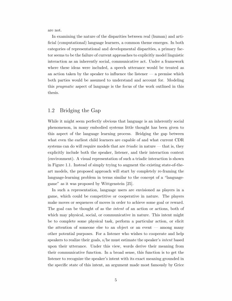
(environment). A visual representation of such a triadic interaction is shown
in Figure 1.1. Instead of simply trying to augment the existing state-of-the-
art models, the proposed approach will start by completely re-framing the
language-learning problem in terms similar to the concept of a “language-
game” as it was proposed by Wittgenstein [25].
In such a representation, language users are envisioned as players in a
game, which could be competitive or cooperative in nature. The players
make moves or sequences of moves in order to achieve some goal or reward.
The goal can be thought of as the intent of an action or actions, both of
which may physical, social, or communicative in nature. This intent might
be to complete some physical task, perform a particular action, or elicit
the attention of someone else to an object or an event — among many
other potential purposes. For a listener who wishes to cooperate and help
speakers to realize their goals, s/he must estimate the speaker’s intent based
upon their utterance. Under this view, words derive their meaning from
their communicative function. In a broad sense, this function is to get the
listener to recognize the speaker’s intent with its exact meaning grounded in
the specific state of this intent, an argument made most famously by Grice
5
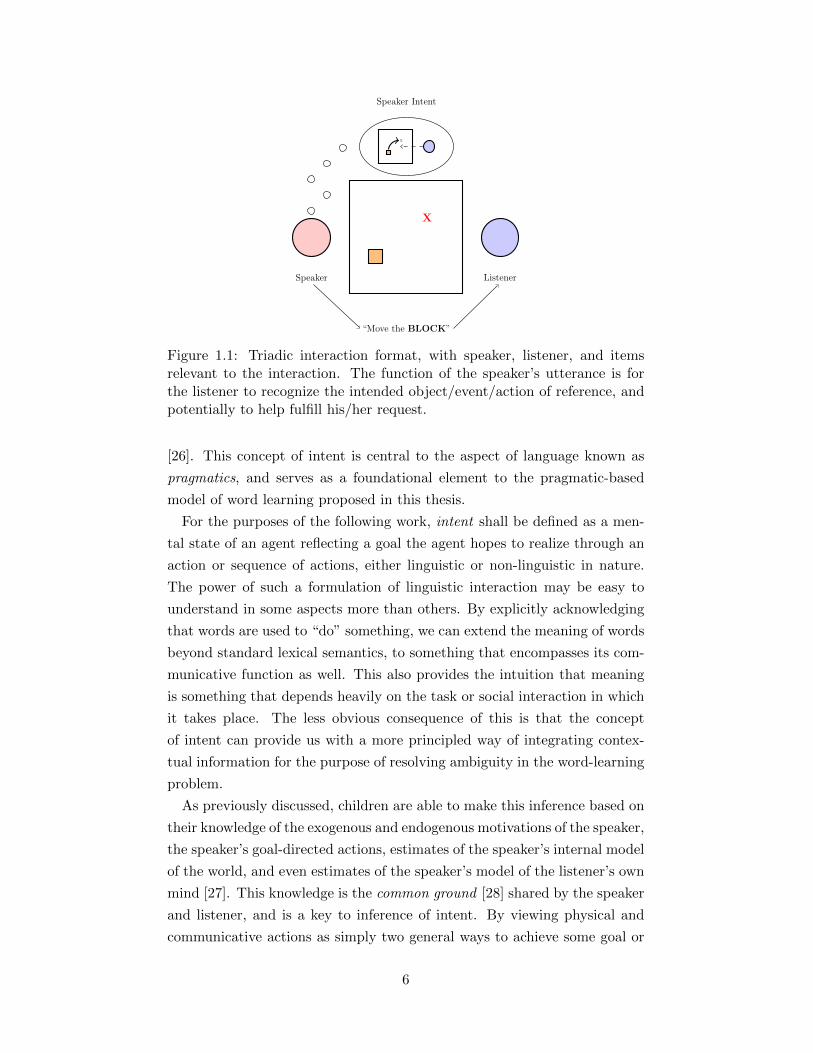
X
X
“Move the BLOCK”
Speaker Listener
Speaker Intent
Figure 1.1: Triadic interaction format, with speaker, listener, and itemsrelevant to the interaction. The function of the speaker’s utterance is forthe listener to recognize the intended object/event/action of reference, andpotentially to help fulfill his/her request.
[26]. This concept of intent is central to the aspect of language known as
pragmatics, and serves as a foundational element to the pragmatic-based
model of word learning proposed in this thesis.
For the purposes of the following work, intent shall be defined as a men-
tal state of an agent reflecting a goal the agent hopes to realize through an
action or sequence of actions, either linguistic or non-linguistic in nature.
The power of such a formulation of linguistic interaction may be easy to
understand in some aspects more than others. By explicitly acknowledging
that words are used to “do” something, we can extend the meaning of words
beyond standard lexical semantics, to something that encompasses its com-
municative function as well. This also provides the intuition that meaning
is something that depends heavily on the task or social interaction in which
it takes place. The less obvious consequence of this is that the concept
of intent can provide us with a more principled way of integrating contex-
tual information for the purpose of resolving ambiguity in the word-learning
problem.
As previously discussed, children are able to make this inference based on
their knowledge of the exogenous and endogenous motivations of the speaker,
the speaker’s goal-directed actions, estimates of the speaker’s internal model
of the world, and even estimates of the speaker’s model of the listener’s own
mind [27]. This knowledge is the common ground [28] shared by the speaker
and listener, and is a key to inference of intent. By viewing physical and
communicative actions as simply two general ways to achieve some goal or
6
intent, knowledge acquired about one can be used to constrain the learning
problem in the other. Learning the meaning of words is just one aspect of
the overall process of construction and adaptation of this common ground
during social interaction.
1.3 Purpose and Contribution of This Thesis
The fundamental goal of this thesis is to build a general pragmatic-based
language learning framework that begins to bridge the gap between the
abilities of current cognitive robotics models, and the actual abilities of the
youngest language learners. We have described two primary factors con-
tributing to this gap: representational disparities, what kinds of meanings
can we learn; and developmental disparities, the ways in which we are able
to learn. We have also discussed at a conceptual level a pragmatic frame-
work, based around an intentional agent, which attempts to address some
aspects of each of these issues. As it is unlikely that any computational
model developed herein would be able to emulate a child’s word-learning
abilities with complete accuracy, we will focus instead on capturing a lim-
ited set of developmental abilities demonstrated by early word learners that
are still lacking in current computational frameworks. We will also explore
some basic ways in which the pragmatic model can be used to stretch our
representations of meaning to include pragmatic aspects, such as commands
and requests, in addition to reference.
Generally speaking, the goal of the model presented here is to be capable of
learning perceptually grounded meanings of words for basic objects and/or
events, specifically in cases of referential ambiguity or non-ostentation, us-
ing various inferential abilities seen in humans. These include both the
cross-situational statistics and lexical contrast techniques already seen in the
computational literature, as well as the inference of intent from goal-directed
actions, understanding of task structure, and knowledge about physical con-
straints. Furthermore, we seek to construct our computational framework
in such a way that allows our agent to reason about its role in the inter-
action, use this ability to aid in actively resolving ambiguity, and through
this, begin to understand the functional aspects of word meaning.
In addition to these specific experimental goals, we also impose a set
of guiding restrictions on the computational models we use to keep them
in line with basic principles of cognitive development. First, preference
will be given to using techniques and algorithms that learn in an online
7
manner whenever possible, with as little supervision as possible with respect
to model structure. Second, the models and algorithms used should be
designed to be ultimately evaluated in real-world experimental human-robot
interaction scenarios, in which noisy sensor data is the primary input and
the only truly observable quantity.
To this end, we present a computational framework, based on statistical
techniques of decision and control in addition to more traditional meth-
ods for speech and language processing, for the acquisition of perceptually
grounded word meanings using pragmatic principles. By modeling language
as a purposeful behavior that is embedded within a social interaction, we
develop and apply techniques for inverse planning to understand the goals
or intents that drive human behavior, which ultimately enables our agent
to capture the kind of pragmatic inference abilities that are crucial to child
word learners. Through its application to a set of human-robot interaction
experiments, we intend to demonstrate the following contributions of this
framework to current body of cognitive robotics systems for grounded word
learning:
• A set of computational models and algorithms for basic grounded word
learning that is inherently pragmatic and triadic.
• The ability to learn word meanings in situations of referential ambigu-
ity from novel contextual information about the intentional structure
of interactions.
• A representation of linguistic meaning that is capable of incorporating
aspects of a word’s communicative function or use.
• The ability of our agent to apply understanding of functional aspects
of language in order to actively guide process of word learning.
1.4 Thesis Organization
The rest of this thesis will proceed as follows. Chapter 2 contains a review
of the relevant background material from the fields of cognitive robotics,
developmental psychology, and machine learning, which includes an overview
of topics from stochastic planning, as well as game theory. Chapter 3 details
the core computational model and learning algorithms that comprise the
pragmatic engine. The framework for integrating perceptual capabilities
into the pragmatic model is presented in Chapter 4. The overall cognitive
8
architecture to be used in the human-robot interaction experiments, which
includes the integrated pragmatic-perceptual framework, as well as various
low-level signal processing and support algorithms, is outlined in Chapter 5.
Chapter 6 describes the set of human-robot interaction experiments, details
their setup, and presents and analyzes their results. In this chapter we also
compare our work to other related research, and we discuss some of the
limitations and issues with our model. Finally, the contributions of this
thesis, and potential paths for future research are discussed in Chapter 7.
9
CHAPTER 2
REVIEW OF RELATED RESEARCH
2.1 Embodied Systems for Linguistic Interaction
The view that understanding the cognitive abilities of humans means also
understanding the physical systems and processes that underly them was
not lost on many of the early pioneers in artificial intelligence. In his 1950
paper [29], Alan Turing proposes that in order to actually create a ma-
chine capable of passing the Turing Test, a developmental approach might
be preferable: “Instead of trying to produce a programme to simulate the
adult mind, why not rather try to produce one which simulates the child’s?”
He goes on to suggest that this learning could be achieved through use of
something like an embodied agent. Around the same time, Norbert Wiener
helped to shape the field of cybernetics around the study of how learning and
feedback were supported and limited by the structure of their biological sys-
tems, i.e. their bodies [30, 31]. For Wiener and others who understood the
importance of embodiment, cognition is not a set of fixed, isolated abilities,
but rather a process with many different and highly interconnected aspects,
which all continually adapt together with feedback from one another and
the environment.
Under such a view, traditional ASR systems are limited in their linguistic
abilities as far as they are limited in their general cognitive abilities. For
many who consider cognition to be embodied, it would only be obvious that
a system without perceptual representations of the world, such as vision
or motor function, would also be incapable of effectively processing the se-
mantic aspects of language. Systems without any kind of social or affective
sense would likewise be unable to operate with humans at a pragmatic level.
Even for systems endowed with fixed corpora of semantic and pragmatic
knowledge by experts, the extremely limited scope of their understanding
relegates them to narrowly defined application domains. Therefore, if we see
that the physical disparity between humans and machines may be in some
part responsible for their cognitive disparities, a reasonable approach might
10
be to first bring the embodiment of our artificial agents closer to that of
humans.
2.1.1 Cognitive Developmental Robotics
Cognitive developmental robotics (CDR) is the result of applying such a
philosophy to real-world systems. However, CDR does not simply entail
expansion of the previously discussed expert knowledge bases to include in-
formation about additional sensory inputs. Rather, it takes into account
the dynamic properties of adaptation and learning that are every bit as
fundamental to the formation of the cognitive faculty as its physical form.
CDR focuses on creating artificial cognitive capabilities that emerge through
the gradual, continuous developmental processes of learning and adaptation,
structured by the agent’s environmental and social interactions, as experi-
enced through the sensorimotor system (for a more general overview of CDR
and other embodied approaches, see [1, 2, 3]).
Even as a relatively new area of research, CDR systems have already been
able to emulate a number of very basic and very important cognitive func-
tions, which almost every human child masters with little effort, but were
not considered under traditional AI paradigms. These include core abilities
like joint attention [32], the acquisition of reaching and grasping skills [33],
and the representation and learning of affordances [34, 35], to name only a
small fraction. While these skills may seem extremely rudimentary in com-
parison to the highly developed and complex faculty of adult language, to
those following a paradigm of embodied cognition, the latter is only made
possible by the former. Without these core capabilities, the scope of natural
language interaction with machines will continue to be limited to passive
speech-to-text transcription devices, with no sense of what language means
(semantics), or how it can be used (pragmatics).
Because of the new possibilities that its approaches offer, a primary sub-
ject of interest in the area of CDR has become language, and in particular,
the topic of language acquisition receives a great deal of attention. The
advantages of a more complete sensorimotor system and real-world phys-
ical embodiment have allowed researchers to begin exploring representa-
tions of semantic and pragmatic aspects of language, typically off limits to
speech-only ASR systems. Machines now have the opportunity to be active
participants and learners in the same real-world environments and social
interaction scenarios as the children they seek to emulate.
One of the most significant capabilities of the CDR approach is that it has
11
allowed researchers to address the long-standing problem of symbol ground-
ing. In the context of language, the problem of symbol grounding is fun-
damentally one of how linguistic symbols acquire their meaning [36]. The
history of artificial intelligence has been dominated by approaches where the
meaning of a linguistic symbol was itself grounded (by an expert) in another
symbol upon which some fixed set of logical operations could be performed
[37]. But the grounding of linguistic symbols in other kinds of symbols
simply leads to problems of infinite regress, as most famously pointed out
by John Searle in his Chinese Room thought experiment [38]. According
to those taking an embodied view of cognition, meaning instead should be
grounded ultimately in perceptual experiences, supported by a sensorimotor
system, as is thought to be the case in humans.
2.1.2 Embodied Platforms for Natural Language
Initial experiments using embodied platforms to explore the issue of symbol
grounding focused primarily on the association between sets of basic objects
and the words describing them. The fundamental practical issues were the
construction of perceptual (usually speech, vision, or action) representations
from sensory data, and the learning of associations between these perceptual
categories. Experimental scenarios consisted of an adult tutor presenting an
object to the robot learner for visual inspection while simultaneously giving
the word for the object as speech [39, 5, 40, 7]. Associations were acquired
gradually, mostly by machine learning techniques based on statistical mod-
els. For these experiments, the robot was largely a passive and motionless
agent, requiring an embodiment no more complex than a camera and mi-
crophone.
After the accomplishments of these initial systems, new frameworks and
experiments were developed using representations of motor function to ex-
pand symbol-grounding abilities to include words describing actions and
spatial relationships. One of the earliest experiments by Sugita and Tan
[41] involved a mobile robot that was able to ground a small set of action
and color words, and use them to compose simple two-word sentences with
a recurrent neural network. In another series of experiments by Takano and
Nakamura [42, 43], the authors developed a system through which a set of
motion primitives were autonomously extracted from motion capture data
and incrementally associated with linguistic symbols. Following the initial
success of these and other similar experiments [8, 44, 45, 46], there has been
a steadily increasing interest in using robots to study the special interaction
12
between language and action during cognitive development [47]. Indeed, re-
cent results from neuroscience and psychology have demonstrated the close
relationship between internal representations for language and action, as in
the case of the discovery of so-called motor neurons [48, 49] and observation
of Action Compatibility Effects (ACE) [50].
One particular example of experiments exploring the interaction between
action and language representations are those dealing with grounding trans-
fer. In these experiments, basic action-word groundings are exploited to
transfer meaning to new words describing complex behaviors, without the
need for direct representation or even demonstration of the behavior. In one
experiment, Cangelosi [8] showed that an artificial agent could use previous
knowledge of action-word pairings to learn multi-step actions from verbal
instruction by transferring the existing groundings of component words to
the new action. Work in our own lab [10] improved on the previous ar-
tificial neural network-based approach by using a generalized, dynamically
expanding perceptual representation built on stochastic models, which was
able learn both compositionally and hierarchically organized behaviors.
Despite such incremental improvements in representational complexity,
most of the artificial agents produced have focused primarily on learning
words for objects (and other vision-related concepts like shape, color, etc.
[51, 12]) and basic actions. More recent work has succeeded in learning
additional words relating to more abstract concepts such as affordances [35]
and affected behaviors [44] of objects, as well as spatial relationships [11].
Words for which our notions of meaning are less easy to connect to specific
perceptual symbols, such as “no”, are only beginning to be explored by
researchers in this area [52]. Similarly, there has been little work in exploring
the relationship between word meaning and use — a concept which will have
to be an intrinsic feature for any future model hoping to represent functional
utterances like negation.
Beyond the addition of richer and more complete sensorimotor informa-
tion, other work has sought to bring more realism to the actual learning
scenarios used in such experiments. Most, if not all, of the work mentioned
so far was designed for and evaluated in contexts where the agent always
knows what object the sample word is referring to. However, in real-world
situations, young children are able to quickly and accurately learn words in
a wide range of scenarios where referents are highly ambiguous. This has
produced many different computational approaches which primarily have
attempted to integrate heuristic principles for resolving ambiguity in very
specific scenarios, or have used large training corpora in order to glean sta-
13
tistical regularities.
One of the most popular among these is the use of so-called “cross-
situational statistics” [4]. In these approaches, observations across multiple
episodes are collected, and the agent learns word-referent associations by
computing the statistical regularities of word-referent co-occurrences. Accu-
racy is further improved through the integration of various heuristics thought
to be employed by human learners, such as information about gaze direction
and prosody [4] or the principle of mutual exclusion [53]. However, many
of these methods rely heavily on batch learning techniques, with memory
and processing requirements that may be beyond those exhibited by early
learners. Additionally, social information served generally as a “spotlight”
to improve accuracy of referent inference.
While this information is indeed an important tool employed by early
word learners, in these examples the social dimension of language has in fact
become disembodied. This is because the agent does not see itself or the
speaker as an active, social agent, and does not understand the pragmatic,
communicative aspect of the interaction. Some attempts at incorporating
this interactive aspect have featured robot word learners who ask questions
to resolve referential ambiguity [54]. Others have used models including
representations of the speaker and listener’s beliefs as a way of integrating
pragmatic information in an utterance understanding task [55]. Even so,
the agents in these experiments still lack an explicit understanding of the
goal-directed or intentional nature of linguistic utterances. Experiments by
Frank [56] attempted to improve on previous associative methods [4] by us-
ing explicit models of the speaker’s referential intent to replicate observed
phenomena like mutual-exclusion [18] and fast-mapping [57]. But produc-
ing such results appears to be more dependent on designer-imposed learn-
ing biases and memory/processing requirements, as the model and learning
algorithms still do not give proper treatment to the dynamic, interactive
aspects of real-world language learning. More recently studies [58, 53] have
highlighted the importance of capturing both the dynamic, online process-
ing aspects, as well as long-term statistical regularities, in models of word
learning.
2.1.3 Language, Action, and Intent
In all of these computational models, the notion of intent has either been
left out entirely, or implemented in a way that strips its intuitive role in
understanding purposeful behavior. This is due in large part to the fact that
14
the intent behind language use is rarely just use itself, but rather something
that is often embedded in a social interaction with larger goals. For humans,
the task of understanding language appears to be deeply connected to the
task of understanding action in general, an idea that the embodied approach
of CDR is uniquely suited to explore. And indeed, many techniques and
experiments have recently started to explore this connection in the context
of tasks requiring joint human-robot action.
A framework developed by Taguchi [59] leverages a more complete model
of intent in a word learning task. Their understanding of both agents’ beliefs
and utterances as goal-directed communicative actions allows them to learn
meanings for functional words like “what” and “which”. Unfortunately, their
framework relies on explicit supervision in the form of corrective feedback
from a human tutor, and does not appear to deal with intentional ambiguity.
In other work by Lopes, Cederborg, and Oudeyer [60], an explicit model of
goal-directed behavior is used to learn the meanings of such feedback signals
in the context of a human-robot interaction. In both this and subsequent
experiments [61], this communication model is learned simultaneously with
the structure of the physical task that it is trying to describe. For these
experiments, the focus is primarily on the acquisition of the word mean-
ing models through continuous feedback with sometimes noisy or incorrect
signals. The work that will be presented uses many of the same kinds of
techniques and ideas, but focuses more on the learning of larger task struc-
ture models, and the use of these models to learn word meanings in more
ambiguous and infrequent input.
Less frequently studied is the use of models that understand communica-
tive actions as goal-directed behaviors, and the use of these models to study
the acquisition of word meanings. As we will see in Section 2.2, such an
understanding appears to be critical to the word learning abilities of chil-
dren. The construction of computational models for teleological, or goal-
directed understanding of language has recently begun to pick up interest
[62, 63], but practical algorithms and implementations of these ideas for use
in human-robot interaction experiments is something that remains to be
seen. However, some general frameworks have been proposed, such as Pez-
zulo’s dynamic Bayesian network-based pragmatic engine [62], which will be
used in this work as a basic starting point for the development of our own
model.
Finally, it is also very much worth mentioning a number of cognitive
robotics architectures and experiments for which the attribution and under-
standing of mental states (such as beliefs or intentions) in other agents is a
15
critical component, but do not focus on language acquisition in particular.
The ability of an agent to make this attribution and reasoning is usually
referred to as Theory of Mind, a term with a long tradition of use in the
study of philosophy and psychology. Perhaps the most relevant among these
is Scassellati’s work on development of a Theory of Mind module for use on
the Cog humanoid robotic platform [64], which itself is based on ideas on
the topic of Theory of Mind put forth by Leslie [65] and Baron-Cohen [66].
Central to his framework is the perception and understanding of gaze infor-
mation, something that will also play an important role in some of our own
human-robot interaction experiments presented in Chapter 6. Other cogni-
tive architectures, such as Demiris’s HAMMER architecture [67] or Bicho,
Louro, and Erlhagen’s work based on Dynamic Neural Field representations,
have shown success in applying ideas about social and mental reasoning for
the understanding of actions and behaviors in real-world interaction exper-
iments.
It is hoped that this review has served to underscore the most significant
issues involving current CDR approaches to early word learning, as they
were presented in the introduction. To restate, our view is that they are
of fundamentally two types: those relating to representations of meaning
— what kinds of words can be learned and how they can be used; and
those relating to acquisition of meaning — primarily the problem of how
we can learn words in noisy, ambiguous real-world situations. The goal in
Section 2.2 will be to briefly review the developmental literature relating to
early language learning, and explore how ideas from social and pragmatic
theories of early language acquisition might be used to structure and guide
development of a new computational framework.
2.2 Pragmatic Models of Language Acquisition
One example of traditional reasoning behind how children come to learn the
meanings of words was given by Augustine [68], later to be used by Ludwig
Wittgenstein in framing his own foundational work on the philosophy of
language [25]:
When they called anything by name, and moved the body to-
wards it while they spoke, I saw and gathered that the thing they
wished to point out was called by the name they then uttered;
and that they did mean this was made plain by the motion of the
body, even by the natural language of all nations expressed by
16
the countenance, glance of the eye, movement of other members,
and by the sound of the voice indicating the affections of the
mind, as it seeks, possesses, rejects, or avoids. So it was that by
frequently hearing words, in duly placed sentences, I gradually
gathered what things they were the signs of and having formed
my mouth to the utterance of these signs, I thereby expressed
my will.
Wittgenstein notes that the conceptualization of words as merely standing
for things does not begin to encompass all of the things we know as “lan-
guage”. Such a view can not account for words that do not stand for specific
things (e.g. “this/that”, “yes/no”), and ignores the effect that aspects like
use and context have on a word’s meaning. We also know that perfect, os-
tensive teaching is not representative of the ambiguous situations in which
children often learn words.
Issues of conceptual representation and referential ambiguity are certainly
not ones faced by computational modelers alone. They are long-standing
open problems in the fields of developmental psychology and linguistics,
and their extensive study in these areas has produced numerous competing
theories about their fundamental nature. Many of the approaches in CDR
have been based on purely associative theories, or expanded theories of asso-
ciation guided by various “principles” and “biases” [69]. These principles are
largely related to the learning of names for objects and other nouns, a trend
that has been reflected in the computational models discussed in Section
2.1. Another competing class of ideas are the so-called “social-pragmatic”
theories of language acquisition [27], which focus on how the social and
pragmatic aspects of communicative interaction are understood and lever-
aged by learners. These treat language acquisition as just one particular
aspect of a more general pragmatic competence, rather than an isolated
cognitive faculty with its own special rules and principles. This aspect is
obviously appealing to robotics researchers pursuing an embodied approach
to language acquisition.
Social-pragmatic theories sometimes differ in various details, but are pri-
marily focused around the core ability of intention reading. At the heart
of this skill is the idea that a child understands human behavior, including
communicative behavior, to be goal-directed (i.e. intentional). These goals
might be to influence physical states of the environment or perhaps mental
states of other social actors (and consequently their actions). In the case
of linguistic communication, the purpose of an utterance is to get the in-
17
terlocutor to recognize one’s own intentional state [26]. When choosing an
optimal action or utterance, the speaker must take into account the assumed
knowledge, beliefs and motivations of the listener, who likewise takes into
account similar information about the speaker in interpreting these utter-
ances. In order to see how these ideas can be used to develop an improved
model of early word learning, we begin exploring them in the context of the
issues of representation and acquisition in early word learners.
2.2.1 Our First 50 Words
As stated, the current focus of language acquisition research in cognitive
robotics has been primarily on learning names for objects, actions and
events, with very little attention given to functional/social words. Many
have justified this focus in the design of such systems by parroting argu-
ments about the actual distributions of word categories observed in a child’s
early lexicon. However, many studies have challenged these estimates [14],
pointing to biases introduced when experimenters consider only utterances
that are referential in nature. Numerous studies have shown that social
and functional words such as “hello”, “yes/no”, etc., constitute a significant
fraction of a child’s first 50 words [13, 14].
These types of words present an additional question that can not be ad-
dressed by nearly any current artificial system: how are meaning and use
related? Even if any current systems were actual active users of language, it
would have almost certainly been as a tool of reference. In fact, reference or
declaration is only one of the ways that young children use language. They
also use language to issue commands [70] and ask for guidance and infor-
mation [71]. Therefore, one response to our question, possibly made most
famously by Wittgenstein [25], is that meaning is use. Within a social-
pragmatic framework, we have noted that utterances are made to get the
listener to recognize the speaker’s intentional state. The intent itself could
be to get the listener to share attention to an object (reference), to get the
listener to take an action (command), or to get the listener to share the
state of his/her own beliefs (question). As will be demonstrated in the ex-
periments in Chapter 7, the ability to understand these kinds of uses can
also affect the ability of a word learner to acquire meanings of words.
18
2.2.2 Early Word Learners’ Use of Social-Pragmatic Principles
With respect to referential ambiguity, “Constraints and Principles” ap-
proaches have focused on crafting a core set of heuristic principles that
can explain a number of observed scenarios where children seem to effort-
lessly and accurately resolve this ambiguity. However, these heuristics are
language-specific, often apply to only a subset of words, and are unable to
adequately explain a number of situations where children resolve ambigu-
ity even when the constraints do not apply. The social-pragmatic approach
gives the explanation that a child’s ability to resolve referential ambiguity
comes from his/her general ability to infer the speaker’s intent based on
shared knowledge of each other’s beliefs, the state of the world, and contex-
tual information about the interaction. The following examples show how
social-pragmatic explanations of various observed phenomena compare to
competing theories, and cases where pragmatic theories can offer explana-
tions where others can not.
One such observation is the apparent use of lexical contrast principles to
infer the proper referent [18]. In these scenarios, the child is presented with
two objects — one with a known label and one without — and the speaker
gives a previously unknown label. Results show that the child often maps
the new word onto the object whose label is not known, a behavior that
many explain as the result of an innate language-specific lexical contrast
principle. This can also be explained as a result of a general pragmatic
competence, whereby the child reasons if the adult intended the child to
attend to the known object, s/he would have used the known label, based
on their shared understanding of the child’s current linguistic knowledge.
The developmental literature is also replete with examples of ways in
which children use their understanding of language users as social actors to
learn the meaning of words — ways which are difficult to explain without
appealing to pragmatic principles, and often times, embodiment. One clear
example comes in a study where an adult used a novel verb before taking
two separate actions [72]. For each action, the adult signified whether it
had been a mistake (“Oops!”), or had gone as intended (“There!”), with
children learning the verb in reference to the intended action. A similar
result was achieved in the context of a finding game [21], in which an adult
referenced an unseen object, hidden in a row of buckets, in advance of their
search for the object. The adult then proceeded to pick objects out of the
buckets, frowning at objects that were not the intended objects, stopping
and smiling when the intended object was found. The children were found
19
to learn the correct referent, regardless of how many distractor objects were
attended to first. In both of these examples, the use of intent by social-
pragmatic theories offers a better explanation than the use of spatial or
temporal proximity provided by associative accounts.
Learners have also been seen to use other information to infer intent in
cases where it is not as explicitly provided as in the previous examples.
Children were thought to be applying knowledge of an adult’s motivation
or preferences in an experiment where the mother, who had previously in-
teracted with three new toys in the presence of her child, was taken out of
the room, and while a fourth, novel toy was presented to the child. Upon
re-entering the room, the mother excitedly produced a label, which the child
took to refer to the novel toy. The child made this inference on the basis of
his knowledge that the mother would only act excitedly toward the object
which was new to her [73]. Other kinds of information for inferring intent
are more transient, such as knowledge of the speaker’s attentive state. A
speaker can use his/her attention to highlight the intended object/event of
reference [74], relying on foundational skills of joint attention.
Finally, children can also infer intent by understanding their active role
in helping speakers achieve their general goals. In one example experiment,
an adult first readied a toy for the child to play with, then presented the
child with a novel object while shifting gaze between the child and the
object. After saying “Widgit, Name”, the child interpreted the utterance
as a request for him/her to use the new object to play with the toy. This
was done in contrast to a scenario where the toy was not first conspicuously
readied for play, and the child learned the word to simply refer to the novel
object [23]. In more recent experiments, children were shown to be able
to use information about the relative physical constraints of the themselves
and the speaker to reason between an ambiguous object requested by the
speaker [75, 24].
2.2.3 Constructing a New Language Engine
But how are these results important, and how can they guide us in the
construction of a new, pragmatics-based computational framework for early
language learning? We see that a wide variety of contextual information
and shared knowledge about the social interaction are required to learn the
meaning of words in cases of ambiguity. But whereas purely association-
based accounts of word learning — and the majority of computational mod-
els — integrate limited, selective bits of this information in specific ways,
20
the pragmatic explanation suggests another organizational principle: intent.
Understanding behavior as being produced to achieve a particular goal, chil-
dren are able to leverage knowledge about the elements of the task structure
that influence the specifics of that behavior (e.g. the goal itself, physical con-
straints, speaker/listener beliefs and preferences) in order to infer a speaker’s
intent even when these behaviors are ambiguous.
These ideas suggest that any computational model that wishes to exploit
these pragmatic principles in order to learn the meanings of words, must also
be capable of representing and learning about the structure of the interaction
in which it takes place. For children, these interactions, sometimes called
“frames” [28], often include everyday, routine activities like diaper changing,
feeding, and playing games. Frames are usually established well in advance
of the word-learning they facilitate. Our pragmatic engine will be developed
around a similar principle of first learning the structure of the interaction,
and then using this knowledge to help resolve ambiguity during the process
of word learning.
2.3 Mathematical Tools for Cognitive Modeling
At the computational level, our methods for implementing this basic prag-
matic competence will be based on statistical models, specifically dynamic
Bayesian models like the hidden Markov model and Markov decision pro-
cess. Additionally, we will draw from traditional techniques for parameter
estimation, as well as more advanced techniques like inverse reinforcement
learning, and more broadly, from research in multi-agent systems and game
theory. The following sections give an overview of these techniques, as they
have been applied in modeling language acquisition and social interaction.
2.3.1 Statistical Machine Learning Fundamentals
Bayes’ Rule and Latent Variable Models
One of the most important techniques in our application of statistical models
is inference of the value of one variable from the value of another. In the
case where these variables are the values of observational data, this can be
viewed as classification. At its heart is the fundamental Bayes’ rule, which
gives the following relationship for two dependent random variables X and
Y :
21
P (X|Y ) =P (Y |X)P (X)
P (Y ). (2.1)
This allows one to estimate the distribution of the variable X in cases where
X can not be directly observed, but Y can. Statistical models with this
structure are often called latent variable models, and are an important tech-
nique for many natural language applications where the values of a discrete
latent variable might correspond to classes of speech features, or associate
multi-modal sensory observations. Relationships and dependencies between
multiple variables can be represented with a directed acyclic graph called a
Bayesian network. When these graphs describe the evolution of variables
over time, they are known as dynamic Bayesian networks, and are of par-
ticular interest in the modeling of time-series data, like speech and action.
Parameter Estimation and Learning
In many applications of statistical models, one does not know in advance the
exact value of the distribution, and would instead like to learn it from some
set of training data. This is the problem of estimating the value of a variable
θ that parameterizes the distribution governing the observed data Y . For
one of the most popular techniques that we will focus on here, the estimate
is made based on the parameter’s likelihood of generating the training set
Y = y0, y1, . . . yT . Assuming individual observations to be independent
and identically distributed (and consequently, the joint distribution to be
factorable), the maximum likelihood estimate (MLE) of the parameter, θML,
can be calculated by maximizing the log-likelihood function over the data:
θML = argmaxθ∈Θ
T∑t=0
log [P (yt|θ)] . (2.2)
For certain forms of the probability mass or distribution function p(y|θ),the optimization can be computed quite easily. One example might be the
simple Gaussian distribution, where the estimator is given by the sample
mean and sample variance. In cases where the data is complicated in struc-
ture, or part of the data is missing/unobservable — as in the latent variable
models discussed above — more sophisticated techniques are necessary to
perform this optimization. One such class of methods used for hidden vari-
able models are known as the expectation maximization algorithm [76]. The
EM algorithm is an iterative procedure based on the alternation of an expec-
tation (E) step and maximization (M) step. The E-step consists of taking
22
the expected value of the log-likelihood function over the hidden data set
X, given the observed data set Y and the current estimate of the parameter
θ(t):
Q(θ|θ(t)) = EX|Y,θ
[logP (Y,X|θ)|Y , θ(t)
]. (2.3)
In the following M-step, the new parameter value θ(t+1) is set to the value
maximizing the current Q(θ|θ(t)).
Another class of techniques we will utilize for parameter estimation are
the stochastic gradient descent (SGD) methods. Techniques of this type are
aimed at optimizing objective functions that can be expressed as sums of
differentiable functions, such as the log-likelihood function (equation 2.2).
Using a standard gradient descent method requires calculating the gradient
of each term in the sum, with respect to each parameter in the parameter
set. SGD limits this operation to a single data point or a small subset of
data points at one time. This means, as opposed to EM techniques which
require the complete observation set to calculate parameter estimates, SGD
allows the model to be trained online, as data samples are gathered. The
update rule for the ML estimate of θ using one-step SGD might look like:
θ(t+1) = ΠG
(θ(t) + εt∇ log
[P (yt|θ(t))
]). (2.4)
In the case of constrained optimization, the operator ΠG is used to represent
the projection of the parameter estimate back onto the allowable constraint
set after each gradient step.
Stochastic gradient algorithms have a number of drawbacks — one of the
most significant is the need for proper setting and control of the learning rate
in order to achieve acceptable performance. However, many of these issues
can be mitigated using a wide variety of heuristics and modifications to the
standard algorithm. But most importantly, the online and adaptive capa-
bilities, combined with their simplicity, make SGD techniques particularly
attractive for many of the learning tasks presented in this thesis.
Hidden Markov Models
A Hidden Markov Model (HMM), an extension of the basic Markov model,
is a dynamic Bayesian network that is commonly used in modeling data
with both spatial and temporal characteristics, such as speech and action.
HMMs are composed of an underlying unobservable Markov process, Xt
and an observable process, Yt. The unobservable process is parameterized
23
by initial state distribution π and transition matrix A, where:
[a]ij = P (Xt+1 = j|Xt = i), (2.5)
πi = P (X1 = i). (2.6)
The distribution of the observable process at each time t is a stochastic
function of the state of the Markov process at that time. This observation
variable may be discrete, in which case it can be parameterized by the
stochastic matrix [b]jk = P (Yt = k|Xt = j), or continuous, in which case
it is often drawn from a Gaussian (or mixtures of Gaussian) distribution,
parameterized by θ = µj ,ΣjNj=0, where µj ∈ Rd is the mean vector and
Σj ∈ Rd×d is the covariance matrix.
Typically the three canonical problems associated with HMMs are the
problems of classification, state estimation, and parameter estimation [77].
Classification refers to the problem of calculating the probability that a
particular parameter set produced a given observation sequence. This cal-
culation is often performed by means of the forward-backward algorithm [78].
This forward algorithm allows for recursive calculation of the joint probabil-
ity of a particular value of the hidden state along with all observations up
to time t. Likewise, the joint probability of all observations from t+1 on up
to T , given a specific value of the hidden state, can be calculated recursively
by the backward algorithm. These recursions are given in the following:
αt+1(j) = P (y1, . . . yt+1, Xt+1 = j|θ)
=
[n∑i=1
αt(i)aij
]fj(yt+1|θ) (2.7)
βt(i) = P (yt+1, . . . yT |Xt = i, θ)
=n∑j=1
aijfj(yt+1|θ)βt+1(j). (2.8)
Initial values for the forward probabilities are set to α1(j) = πjfj(y1), and
backward probabilities are set to βT (i) = 1 for all i. Calculating the corre-
sponding most likely hidden state sequence of the model can be done using
the Viterbi algorithm [79], a special case of the larger class of dynamic pro-
gramming algorithms.
There are many ways of approaching the final task of parameter estima-
24
tion, but two of the most popular techniques are those of the Baum-Welch
algorithm [80] (a special case of the EM algorithm) and stochastic gradient
descent [81, 82]. Both methods have their own advantages and disadvan-
tages. The Baum-Welch algorithm carries the primary advantage that each
iteration of the algorithm is guaranteed to increase the value of the objective
function. Its downside is that it requires the entirety of the training data to
be present, a constraint which may not be suitable for online/incremental
learning applications. The alternative is to use a stochastic gradient descent
algorithm, such as the recursive maximum likelihood estimation (RMLE)
algorithm [82]. Here, the parameter set θ is updated at each time step in
the direction of the gradient of the incremental score:
θt+1 = ΠG (θt + εt∇ log [P (yt|yt−1, . . . y1, θt)]) , (2.9)
where ΠG is the projection operator on to the manifold of allowable param-
eter sets. The advantage here is that training is done online, as each data
point is received. Unfortunately, assuring proper convergence using these
techniques often requires careful tuning of the step size parameter, εt.
Our choice to make use of the HMM in certain aspects of the work de-
scribed in this thesis is based in no small part on its wide application to
the domain of speech recognition, as well as the representation and learning
of gestures and other motor primitives. In speech recognition, the HMM
has long been a standard model for representing nearly every level of the
language faculty, from fundamental phonological and morphological units
[37, 83], to simplified syntactic structures such as context-free grammars
[84]. This capability in representing time-series data has been just as read-
ily applied to the domains of physical action, of which motor primitives
— the short, reusable movements used to compose more complex gestures
— are particularly interesting to us. Work on the topic of Programming-
by-Demonstration (PbD), where a human tutor manually guides a robot’s
actuators in order to teach it an action, has effectively used HMMs to auto-
matically segment larger gestures into motor primitives [85], incrementally
adding to its action repertoire when unknown primitives are discovered [86].
Further methods have been created for robot learners to generate novel ex-
amples of these learned motor primitives using their corresponding HMM
parameter sets [87]. Previous work in our own lab has made use of this
method and other HMM techniques in action-language integration experi-
ments where a robot could produce complex actions from verbal instruction
using previously learned motor primitive word groundings [10].
25
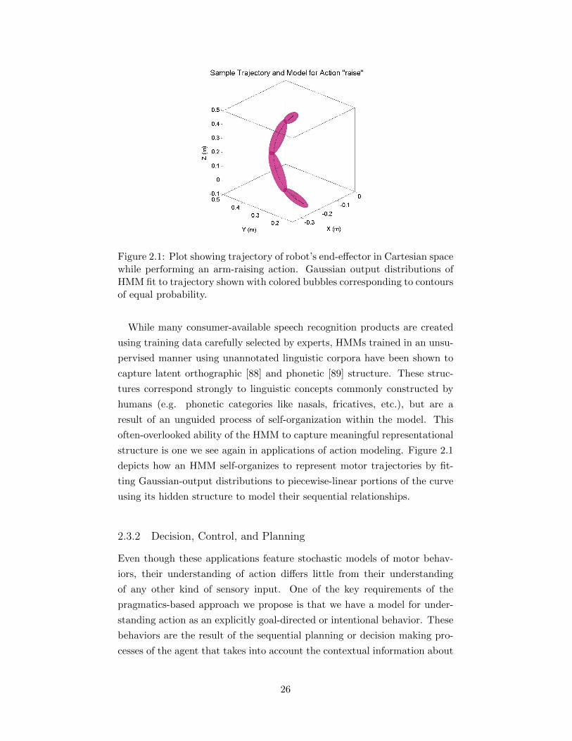
Figure 2.1: Plot showing trajectory of robot’s end-effector in Cartesian spacewhile performing an arm-raising action. Gaussian output distributions ofHMM fit to trajectory shown with colored bubbles corresponding to contoursof equal probability.
While many consumer-available speech recognition products are created
using training data carefully selected by experts, HMMs trained in an unsu-
pervised manner using unannotated linguistic corpora have been shown to
capture latent orthographic [88] and phonetic [89] structure. These struc-
tures correspond strongly to linguistic concepts commonly constructed by
humans (e.g. phonetic categories like nasals, fricatives, etc.), but are a
result of an unguided process of self-organization within the model. This
often-overlooked ability of the HMM to capture meaningful representational
structure is one we see again in applications of action modeling. Figure 2.1
depicts how an HMM self-organizes to represent motor trajectories by fit-
ting Gaussian-output distributions to piecewise-linear portions of the curve
using its hidden structure to model their sequential relationships.
2.3.2 Decision, Control, and Planning
Even though these applications feature stochastic models of motor behav-
iors, their understanding of action differs little from their understanding
of any other kind of sensory input. One of the key requirements of the
pragmatics-based approach we propose is that we have a model for under-
standing action as an explicitly goal-directed or intentional behavior. These
behaviors are the result of the sequential planning or decision making pro-
cesses of the agent that takes into account the contextual information about
26
the current state of the world, other agents, and the uncertain dynamics
of its environment. The Markov decision process (MDP) is a well-studied
stochastic model that is capable of capturing many aspects of such problems.
Markov Decision Processes
We define an MDP using a tuple of four elements: a state space S =
s1, s2, . . . sN, an action space A = a1, a2, . . . aM, a state-action tran-
sition model T (s, s′, a) = P (St+1 = s′|St = s,At = a), and finally a reward
function R(s, s′, a) which gives the immediate reward received at state s′
when transitioning from state s with action a. This framework is an ex-
tension of the basic Markov model that allows us to model active agents,
who produce behaviors to maximize some reward. Analogously, the hidden
Markov model can be extended in the same way, yielding a new model called
the partially observable Markov decision process (POMDP), with the added
element of an observation model Ω(o|s′, a) = P (Ot+1 = o|St+1 = s′, At = a).
For the purposes of this thesis, however, we will only consider fully observ-
able MDPs.
Of particular interest in this application is the representation of the reward
function. Through the reward, it is possible to encode the goals or intentions
that drive the behaviors of a rationally acting agent. As mentioned previ-
ously, one such goal might be to reach a particular state, in which case an
indicator function for that particular state, I(s∗), could be used to represent
the reward function. Often, especially in scenarios where the state space is
extremely large or heavily factored, the goal is some derived feature present
in a number of states. In these cases, a common approach is to parameterize
the reward function as a linear combination of some set of features:
R(s, s′, a) = θTψ(s, s′, a), (2.10)
where ψ : S × S × A → Rf , and θ ∈ Rf . Further on in this thesis, we will
also discuss rewards and feature representations that depend on only the
current state and action (ψ(s, a)), or simply the current state (ψ(s)). Such
a representation of the reward function will prove to be especially useful
when approaching the inverse reinforcement learning problem in situations
where |S × S ×A| f .
27
Optimal Planning with MDPs
In nearly all applications of MDPs, the primary goal is to find a policy
function π : S → A that maximizes some objective function. The policy
function specifies the action a that the agent will choose when in state s.
This objective function is usually chosen to be an expected discounted sum
of the reward function, often referred to as the return, over some potentially
infinite horizon:
Rt =∞∑τ=0
γτR(St+τ , St+τ+1, At+τ ), (2.11)
where γ ∈ [0, 1) is known as the discount parameter. The most well-known
technique for approaching this problem is the dynamic programming tech-
nique developed by Bellman [90]. This technique has many different variants,
which center around the calculation of two quantities: the policy function
π(s) and the value function under that policy V π(s):
π(s) := argmaxa∑s′
T (s, s′, a)[R(s, s′, a) + γV (s′)
], (2.12)
V π(s) :=∑s′
T (s, s′, π(s))[R(s, s′, π(s)) + γV (s′)
], (2.13)
= Eπ
[R|s0 = s, π
]. (2.14)
As is shown here, the value function is the expected value of the future
reward (return), given a particular policy. The optimal policy, which we
denote as π∗(s), is defined as the policy that maximizes the value function
for all states. This optimal policy can be found through various applications
of equations (2.12) and (2.13) above. In the technique of value Iteration, the
policy update equation is substituted into the value function calculation to
yield the combined equation
V (s) := maxa∑s′
T (s, s′, a)[R(s, s′, a) + γV (s′)
], (2.15)
which is iteratively updated for all states until convergence. In the Policy
Iteration version of the algorithm, a policy update step is performed, after
which value function updates are iteratively made until convergence. This
procedure is then repeated until the policy update step results in no change
for all states.
Rather than iteratively calculating equation (2.13), the value of V π(s) for
28
a particular policy can be obtained through linear methods. Consider the
case where the reward is a function of only the current state and action. We
can then use a vector notation for the reward and value functions under a
particular policy: V π, Rπ ∈ R|S|, where Rπ(s) = R(s, π(s)). We also denote
Tπ as the |S| × |S| stochastic matrix with entries given by T (s, s′, π(s)).
Using this notation, equation (2.13) can be expressed and evaluated as:
V π = Rπ + γTπVπ, (2.16)
= (I − γTπ)−1Rπ. (2.17)
We will find this vector formulation and corresponding linear solution to
be useful in the discussion of the inverse reinforcement learning problem
presented later in this section.
Reinforcement Learning and Applications
But what about a scenario where the agent does not know the transition
model or the reward function in advance? This is the problem of reinforce-
ment learning (RL). One solution might be to use a simple Monte Carlo
method to evaluate the equations above. First, let us define a helpful in-
termediate quantity Qπ(s, a), the action-value function (more commonly
referred to as the Q-function) as:
Qπ(s, a) = E
[ ∞∑t=0
Rt|s0 = s, a0 = a, π
](2.18)
=∑s′
T (s, s′, a)[R(s, s′, a) + γQπ(s′, π(s′))
]. (2.19)
We also denote Q∗(s, a) to be the Q-function under the optimal policy π∗(s).
Starting with a basic policy iteration algorithm, the Qπ function can be es-
timated by generating a set of training episodes under policy π with random
initial state-action pairs (s, a), and by simply averaging over the resulting
returns sampled for each episode. This estimated Qπ(s, a) can then be used
easily to evaluate V π(s). However, one problem with this algorithm is that
it is inefficient as it spends too much time evaluating each (sub-optimal)
policy. One way to improve this might be to perform a policy update after
every training episode.
A more pressing problem though is the fact that the return sampled from
29
a training episode is only used to update a single state-action pair. The
technique of temporal difference (TD) learning developed by Sutton and
Barto [91] addresses this problem by using the recursive Bellman equation
to update the value function after each time step of an episode:
V (st) = V (st) + η [rt+1 + γV (st+1)− V (st)] , (2.20)
where rt+1 is the immediate reward experienced after leaving state st, and
the parameter η is the learning rate. As stated, the TD learning algorithm
only estimates the value function for a fixed policy π, and does not address
the issue of how to update the policy function π. As with the previous Monte
Carlo methods, our approach is to apply the TD learning technique to es-
timate the action-value function Qπ(s, a). The result is called the SARSA
algorithm, as it requires not only the current state-action pair and expe-
rienced reward, but also the next state-action pair, in order to realize the
recursive bootstrapping procedure of the TD algorithm:
Q(st, at) = Q(st, at) + η [rt+1 + γQ(st+1, at+1)−Q(st, at)] . (2.21)
SARSA is referred to as an on-policy method, as the policy used in evalu-
ating the action-value function is the same one used for choosing behaviors.
However, it might also be desirable to learn about other policies for control,
including the optimal policy. The most popular of the off-policy TD learn-
ing algorithms is the Q-learning algorithm [92], which updates its Q-function
according to:
Q(st, at) = Q(st, at) + η[rt+1 + γmax
aQ(st+1, a)−Q(st, at)
]. (2.22)
In this particular form of the Q update, we see that we are in fact approxi-
mating the optimal Q-function Q∗ directly. Unfortunately, both Q-learning
and TD-learning suffer from many issues of finiteness, convergence, and in-
stability. Much of the current research focuses on improving performance in
these areas, and has produced extensions to the vanilla TD and Q learning
algorithms, such as function approximation, as well as mixing of TD and
Monte Carlo methods as in TD(λ) and Q(λ) [91].
For many applications in cognitive developmental robotics, temporal difference-
style methods have been a popular choice due to their focus on gradual
learning. Reinforcement learning approaches have been successfully applied
30
to learn basic motor primitives [93] and locomotion [94]. RL methods have
also been used to develop more socially oriented skills. One example in this
area was an experiment on developing joint attention [95], in which gaze-
direction was learned by using TD-learning to build a map between head
pose and target locations. Another example application was to the problem
of imitation learning [96], which included the task of learning to imitate
observed effect. This same paper also addresses the related but distinct
problem of learning the tutor’s intended goal from his or her actions, even
when these actions are incomplete or unsuccessful. Approaching this second
task, while much more challenging, is nevertheless a critical component in
developing our pragmatic model for early language acquisition.
Inverse Reinforcement Learning
The problem of inferring the reward function that an agent is attempting
to maximize from demonstrations of its behavior is known as the problem
of inverse reinforcement learning (IRL). The IRL problem is fundamen-
tally ill-posed, as there are infinitely more reward functions for which a set
of observed state-action trajectories is optimal [97]. Given this, most ap-
proaches to the IRL problem attempt to constrain or narrow the solution
space by favoring particular reward functions. These techniques fall under
two general categories. The first consists of gradient-based methods that
minimize some dissimilarity function between the empirically observed pol-
icy and the optimal policy under a particular reward. The second category
includes those techniques that cast IRL as a Bayesian inference problem,
and use Monte Carlo methods to estimate a posterior distribution over the
reward function. Each class of algorithms has a number of advantages and
disadvantages, which will be discussed briefly here.
Gradient techniques are some of the earliest and most varied approaches
to the IRL problem. In their review of IRL algorithms, Neu and Szepesvri
make the case that these methods all fundamentally attempt to find a reward
function such that the dissimilarity between the trajectories produced under
the reward’s optimal policy and the observed trajectories is minimized [97].
Using the representation of the reward function from equation (2.10), the
problem is formulated thusly:
θ∗ = argminθ
J(θ;OD), (2.23)
where OD = ξ1, ...ξN is the complete set of example demonstrations, and
31
ξi = st, atTit=0 denotes the state-action sequences that are the individual
observations. The exact form of the dissimilarity function J(θ;OD) being
minimized is what distinguishes the various algorithms of this type, which
are numerous [98, 99, 100, 101, 102]. These methods each provide advantages
and disadvantages with respect to computational simplicity, robustness to
noise, sensitivity to scaling, and generalization, among many other aspects.
The particular approach adopted in this thesis follows from the maximum-
likelihood gradient IRL method used by Lopes et al. [102]. In this case,
the reward parameter is estimated through a similarity function: the log-
likelihood. We use (st, at) to denote a single state-action pair within the
set of observed trajectories OD. Assuming a stationary policy of the agent
over the observations, the likelihood can be factored into probabilities of
individual state-action pairs:
θ∗ = argmaxθ
logP (OD|θ),
= argmaxθ
log∏t
P (at|st, θ),
= argmaxθ
∑t
logP (at|st, θ). (2.24)
Under the standard MDP formulation, the action taken at a particular
state is fixed if an agent is acting in a way that maximizes expected reward.
In order to find a gradient procedure for maximizing this function, however,
we must switch to a differentiable, stochastic policy function. Under the as-
sumption — ubiquitous to nearly all IRL techniques — that the probability
with which an agent takes an action in a particular state is proportional to
the optimal expected return of that decision, the stochastic policy πθ(a|s)is modeled as a Boltzmann or Softmax distribution:
πθ(a|s) , P (At = a|St = s, θ), (2.25)
=eαQ
∗(s,a;θ)∑a′ e
αQ∗(s,a′;θ), (2.26)
where Q∗(s, a; θ) denotes the optimal Q-function for reward parameter θ.
For the sake of simplicity, we have adopted the slight abuse of notation of
[97], using πθ(a|s) to refer to the optimal stochastic policy under θ, in place
of π∗θ(a|s). The parameter α is used to control how strongly the agent favors
actions with greater utility.
32
This softmax formulation of the policy allows the gradient of equation
(2.24) to be taken with respect to the parameter vector θ:
∇θ
[∑t
logP (at|st, θ)
]=∑t
1
πθ(at|st)∇θπθ(at|st). (2.27)
Alternatively, the log-likelihood and its gradient can be reformulated by
replacing the summation over all points in the dataset with a summation
over all possible state-action pairs in the given MDP:
∇θ logP (OD|θ) = ∇θ
[∑S×A
µE (s)πE (a|s) log πθ(a|s)
]
=∑S×A
µE (s)πE (a|s) 1
πθ(a|s)∇θπθ(a|s), (2.28)
where µE (s) denotes the normalized empirical state occupancy count, and
πE (a|s) denotes the normalized empirical action probabilities for a given
state, over the demonstration set. Assuming that OD consists of N total
observed state-action pairs (st, at), we define the calculation of these empir-
ical quantities thusly:
µE (s) =∑t
I(st = s), (2.29a)
µE (s) =µE (s)
N, (2.29b)
πE (a|s) =∑t
I(st = s ∧ at = a), (2.29c)
πE (a|s) =πE (a|s)µE (s)
. (2.29d)
Taking the derivative of πθ(a|s) with respect to θ in turn involves cal-
culation of the derivative of Q∗(s, a; θ), which is non-trivial, due to the
dependence of Q∗ on πθ(a|s) itself. Neu and Szepesvri show that for reward
functions of the form given in equation (2.10), this gradient exists and is
given by:
∇θπθ(a|s) = απθ(a|s)
[Ψθ(s, a)−
∑a′
πθ(a′|s)Ψθ(s, a
′)
]. (2.30)
33
The term Ψθ(s, a) is known as the conditional feature expectation, which is
the expected sum of (discounted) features under policy πθ, starting from
initial state-action (s, a):
Ψθ(s, a) = Eπθ
[ ∞∑t=0
γtψ(s, a)|s0 = s, a0 = a
]. (2.31)
These feature expectations can be calculated in a similar fashion to the
iterative estimation of the value function given in equation (2.13).
In this and other gradient IRL approaches, the gradient calculation is used
to successively update the reward parameterization, according to the general
form given in equation (2.4). Most gradient-IRL algorithms require that the
“forward problem” of finding the optimal policy be solved at each step in
order to calculate the gradient, resulting in significantly higher computation
cost in comparison to solving the forward problem alone. Within the family
of methods, there are also trade-offs in performance and speed. Both the
Policy Matching (PM) approach [97] and the ML approach used here have
objective functions that are non-convex, which can lead to suboptimal so-
lutions under gradient approaches. While other methods like MaxEnt [101]
are convex, PM and MLIRL have the advantage of simplicity and intuition
in favoring rewards that reproduce the observed policy. But ultimately,
PM/MLIRL and MaxEnt approaches have both been shown to stand above
most others in terms of performance, with relatively little difference between
the two.
The second class of IRL algorithms are those based in Bayesian infer-
ence. One of the earliest uses of this approach comes from Ramachan-
dran and Amir’s Bayesian IRL formulation [103]. Here IRL is structured
as a Bayesian estimation problem, where the goal is to estimate the poste-
rior distribution over reward functions R (represented as an N -dimensional
vector over the state space), given a sequence of state-action pairs OD =
(s1, a1), (s2, a2), . . . (sT , aT ) generated by an optimally behaving demon-
strator D. The posterior distribution is given by Bayes’ rule:
P (R|OD) =P (OD|R)P (R)
P (OD). (2.32)
This algorithm retains many of the assumptions on the stationarity of
the agent’s policy and form of the stochastic policy that were seen in the
gradient-based IRL approaches. In his paper, Ramachandran shows that the
reward function minimizing the squared-error loss is equal to the mean of this
34
posterior distribution. Clearly for the general case where each R(s) is drawn
from some continuously valued distribution, analytical calculation of the
mean is intractable, requiring the use of Monte Carlo estimation methods.
Because — as in gradient approaches — each sample of the reward requires
re-solving the optimal planning problem of the MDP, the number of samples
necessary for convergence in the BIRL algorithm makes it computationally
prohibitive to use for MDPs with large state spaces. At the same time, the
fact that it estimates a distribution over reward functions, rather than a
single point in the parameter space, makes BIRL more robust to observed
behaviors that are suboptimal.
The general framework of probabilistic inference of goals provided by
BIRL, however, will still prove to be useful in our application. While the
learning of a reward parameter may be more computationally tractable us-
ing gradient IRL, the notion of using a prior distribution over goals gives us
a simple, intuitive way to estimate which of a set of previously learned tasks
or goals an agent is attempting to optimize in a novel observation. In this
way we are able to exploit the usefulness of Bayesian formulation in cases
where the demonstration was inaccurate or incomplete relative to its actual
goal, something that has been seen in a number of applications to intention
inference [102, 104, 105]. Such scenarios are important, as they are very
similar to many of the experimental scenarios discussed in Section 2.2 that
we wish to emulate [20, 21].
2.3.3 Multi-Agent Systems and Game Theory
One final area of interest is the body of research in multi-agent systems,
which fuses the previously discussed statistical models and algorithms with
concepts from the area of game theory. Game theory is the study of behav-
ior and decision making in environments featuring multiple competing or
cooperating agents. For our purposes, we will discuss specific applications
of game theoretic methods and ideas in the areas of linguistics, where it has
seen extensive use in modeling and understanding pragmatics. These ideas
are particularly relevant to our proposed application, keeping in line with
the idea of communicative interactions as language games.
Extensive Form Games
We begin by limiting our focus to so-called extensive form games, where
players make moves sequentially, i.e. one after another [106]. Such games
35
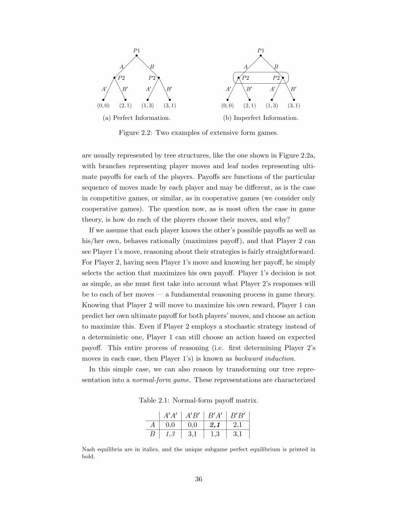
P1
P2
(0, 0)
A′
(2, 1)
B′
A
P2
(1, 3)
A′
(3, 1)
B′
B
(a) Perfect Information.
P1
P2
(0, 0)
A′
(2, 1)
B′
A
P2
(1, 3)
A′
(3, 1)
B′
B
(b) Imperfect Information.
Figure 2.2: Two examples of extensive form games.
are usually represented by tree structures, like the one shown in Figure 2.2a,
with branches representing player moves and leaf nodes representing ulti-
mate payoffs for each of the players. Payoffs are functions of the particular
sequence of moves made by each player and may be different, as is the case
in competitive games, or similar, as in cooperative games (we consider only
cooperative games). The question now, as is most often the case in game
theory, is how do each of the players choose their moves, and why?
If we assume that each player knows the other’s possible payoffs as well as
his/her own, behaves rationally (maximizes payoff), and that Player 2 can
see Player 1’s move, reasoning about their strategies is fairly straightforward.
For Player 2, having seen Player 1’s move and knowing her payoff, he simply
selects the action that maximizes his own payoff. Player 1’s decision is not
as simple, as she must first take into account what Player 2’s responses will
be to each of her moves — a fundamental reasoning process in game theory.
Knowing that Player 2 will move to maximize his own reward, Player 1 can
predict her own ultimate payoff for both players’ moves, and choose an action
to maximize this. Even if Player 2 employs a stochastic strategy instead of
a deterministic one, Player 1 can still choose an action based on expected
payoff. This entire process of reasoning (i.e. first determining Player 2’s
moves in each case, then Player 1’s) is known as backward induction.
In this simple case, we can also reason by transforming our tree repre-
sentation into a normal-form game. These representations are characterized
Table 2.1: Normal-form payoff matrix.
A′A′ A′B′ B′A′ B′B′
A 0,0 0,0 2,1 2,1
B 1,3 3,1 1,3 3,1
Nash equilibria are in italics, and the unique subgame perfect equilibrium is printed inbold.
36
by a payoff matrix, in which rows and columns correspond to the possible
strategies of Player 1 and Player 2 respectively. The extensive form game of
Figure 2.2a has been converted to the example payoff matrix given in Table
2.1, with the elements of Player 2’s policy pairs corresponding to responses
to each of the possible preceding moves of Player 1. In the previous para-
graph, we reasoned that Player 2 would always pick the best response to
Player 1’s action, which is the strategy profile (B′, A′) for Figure 2.2a, and
that Player 1 would choose the best action given her beliefs about Player 2’s
response policy — A in this case. This combined strategy profile is known
as a subgame perfect equilibrium, as the behavior of the players in each sub-
game (subtree) is optimal. Subgame perfect equilibria (SPE) are a subset of
another kind of equilibria known as Nash Equilibria. Nash equilibria (NE)
are values of the combined strategy profile (i.e. elements of the payoff ma-
trix) for which no player can make a unilateral change in strategy that yields
a better payoff for that player. We see in Table 2.1 that there are two such
NE, and that not all NEs are SPEs.
Games of Imperfect and Incomplete Information
What happens if Player 2 is unable to see Player 1’s move? Such scenarios
are called games of imperfect information. In our tree representation, this
is represented by a circle joining a set of a player’s nodes that the player
can not distinguish between (shown in Figure 2.2b), called an information
set. The process of backward induction used above can not see through
such information sets, meaning we can not find a SPE. While backward
induction can not be applied, we can still reason about strategies using
the assumption of mutually understood rationality. In the game shown in
Figure 2.2b, Player 1 would understand that whatever Player 2’s policy
might be, picking A will always yield a greater payoff. Under this, Player 2,
even though he can not see which node of the information set he is at, would
assign a much greater probability that Player 1 had played A, and choose the
policy that maximized his expected reward. The resulting strategy profile
is a perfect Bayesian equilibrium, which is defined over a strategy profile
and a belief system. The PBE is satisfied when strategies are sequentially
rational (i.e. they maximize expected payoff at every information set), and
beliefs are consistent (i.e. probabilities of nodes in an information set given
a strategy profile are computed using Bayes’ rule).
Consider now a third scenario where Player 2 does not know Player 1’s
strategy or payoffs, referred to as a case of incomplete information. In some
37
cases it is possible for this game to be transformed into a game of imperfect
information involving three players, where Player 1 is able to observe Player
0’s move, but Player 2 can not observe the move. Here, Player 0 is usually
taken to represent a choice made by nature that selects Player 1’s type, which
in turn fully defines the payoff function. One game of this form is the class
of signaling games [107]. Signaling games consist of a sender and receiver,
who we denote with σ and ρ respectively, with the sender being of some
type i chosen by nature. Only the sender is able to observe her type, which
upon learning she chooses to take some action a. In a cooperative signaling
game, a is a message visible to the receiver, who then chooses a response d.
As with the game of imperfect information, we wish to apply the concept
of perfect Bayesian equilibrium to our problem, this time in more mathemat-
ical detail. First, we define the beliefs of both the sender and the receiver
over each other’s action strategies. The sender holds a belief about the re-
ceiver’s strategy ρ(a, d), that specifies the probability of the receiver taking
a response d to message a. Being rational, the sender of type i chooses a
signaling strategy that maximizes her expected payoff Uσ(i, a, d) given her
belief ρ:
σ(i) ∈ argmaxa
∑d
ρ(a, d)Uσ(i, a, d). (2.33)
Likewise, the receiver holds a belief µ over the sender’s type given the mes-
sage a that has been received. We similarly consider a rational receiver that
chooses the strategy maximizing his expected payoff Uρ(i, a, d) given the
belief µ:
ρ(a) ∈ argmaxd
∑i
µ(i|a)Uρ(i, a, d). (2.34)
Previously, we noted that two of the conditions of a PBE are that the
players’ strategies maximize the expected payoff, given beliefs over the other
player’s behavior policies. Equations (2.33) and (2.34) satisfy these condi-
tions, known as conditions of sequential rationality, for the signaling game.
The third condition is that the beliefs be consistent, meaning that beliefs
over states in an information set should behave according to Bayes’s rule.
This means that the belief ξ(i|a) is a posterior probability calculated from
the receiver’s belief over the sender’s strategy σ(i, a):
ξ(i|a) =σ(i, a)P (i)∑i′ σ(i′, a)P (i′)
. (2.35)
38
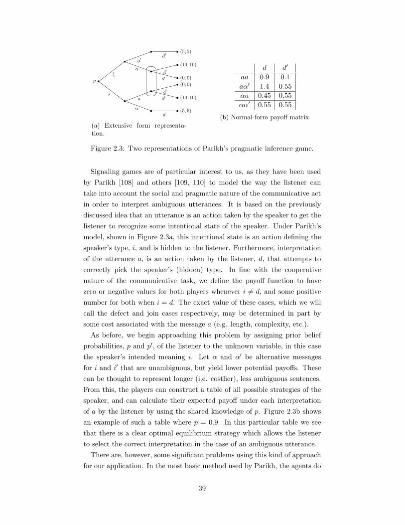
p
(5, 5)d
α
(10, 10)d
(0, 0)
d′
ai
(0, 0)d
(10, 10)
d′a
(5, 5)d′
α′
i′
(a) Extensive form representa-tion.
d d′
aa 0.9 0.1
aα′ 1.4 0.55
αa 0.45 0.55
αα′ 0.55 0.55
(b) Normal-form payoff matrix.
Figure 2.3: Two representations of Parikh’s pragmatic inference game.
Signaling games are of particular interest to us, as they have been used
by Parikh [108] and others [109, 110] to model the way the listener can
take into account the social and pragmatic nature of the communicative act
in order to interpret ambiguous utterances. It is based on the previously
discussed idea that an utterance is an action taken by the speaker to get the
listener to recognize some intentional state of the speaker. Under Parikh’s
model, shown in Figure 2.3a, this intentional state is an action defining the
speaker’s type, i, and is hidden to the listener. Furthermore, interpretation
of the utterance a, is an action taken by the listener, d, that attempts to
correctly pick the speaker’s (hidden) type. In line with the cooperative
nature of the communicative task, we define the payoff function to have
zero or negative values for both players whenever i 6= d, and some positive
number for both when i = d. The exact value of these cases, which we will
call the defect and join cases respectively, may be determined in part by
some cost associated with the message a (e.g. length, complexity, etc.).
As before, we begin approaching this problem by assigning prior belief
probabilities, p and p′, of the listener to the unknown variable, in this case
the speaker’s intended meaning i. Let α and α′ be alternative messages
for i and i′ that are unambiguous, but yield lower potential payoffs. These
can be thought to represent longer (i.e. costlier), less ambiguous sentences.
From this, the players can construct a table of all possible strategies of the
speaker, and can calculate their expected payoff under each interpretation
of a by the listener by using the shared knowledge of p. Figure 2.3b shows
an example of such a table where p = 0.9. In this particular table we see
that there is a clear optimal equilibrium strategy which allows the listener
to select the correct interpretation in the case of an ambiguous utterance.
There are, however, some significant problems using this kind of approach
for our application. In the most basic method used by Parikh, the agents do
39
not form or leverage explicit beliefs about the strategy of the other in their
decision making. For this simple technique to be feasible, it requires that
each possible referent have an unambiguous alternative description. A more
advanced technique might be to use the idea of the perfect Bayesian equilib-
rium to instead have the speaker and listener hold beliefs about the other’s
play. This approach would still entail both agents simultaneously choosing
belief/strategy profiles to coordinate their behavior. For a learning agent,
this is not an applicable solution, as the adult speaker likely already has
a belief in mind about how the listener should respond. One final problem
pointed out in [111] is that there is usually little said about how p is selected.
For our particular application, we find this flexibility to be an advantage,
and will show in our proposed model how this prior probability might serve
as a connection point for integrating knowledge of motivation, beliefs, or
context.
There is much work in game theory that considers agents who can learn.
Nearly all algorithms used fall into one of two categories — fictitious play
and reinforcement learning — both of which model how agents learn over
successive repetitions of a particular game. In fictitious play, an agent keeps
a history of how frequently opponents make a given move, and uses the
derived belief on their stochastic policy to choose a rational strategy. In
reinforcement learning, a history of experienced payoffs is kept and used to
guide the player’s subsequent strategy toward those which have had best
historical utility. Computational models employing reinforcement learning
alone [112], or in combination with fictitious play [113], have been applied
to the case of general signaling games. More interesting yet are learning
algorithms that have been applied to signaling game models of pragmatic
language use [114]. For each of these models, however, the learner is ulti-
mately given access to the speaker’s hidden type or an explicit reinforcement
signal, as well as the received message. Reality is not so forgiving to chil-
dren, who often must learn in situations where true intended referents are
never revealed, and the adult does not provide feedback to their guesses
[115]. While we still find the basic framework of the signaling game to be
useful, we will need to develop our own set of techniques in order to address
the challenges of our specific task.
40
CHAPTER 3
A PRAGMATIC MODEL FOR EARLY WORD
LEARNING
In the introduction of this thesis, a broad set of goals was outlined in order to
guide the construction of a pragmatic model of early word learning. Inspired
by observations of child word learners in the areas of developmental psychol-
ogy and cognitive science, these goals included both desired capabilities to
be replicated by the model, as well as overarching principles regarding the
kinds of techniques to be used in the model. This chapter begins by outlin-
ing our approach at the highest level, and detailing the primary experiments
against which the model will be evaluated. We proceed by presenting the
core pragmatic model, and incrementally extended it in order to meet more
complex goals. At each layer, we provide the mathematical formulation of
the model, derive the associated algorithms for learning and inference, and
discuss how the model applies to the relevant motivating experiments.
3.1 Overview and Motivation
The core problems with current computational models for grounded word
learning, as we have presented them thus far, are of two types: repre-
sentational and developmental. At a high level, we have discussed how a
model based on principles of social-pragmatic theories of language acquisi-
tion might be used to address these issues. While such theories are complex
and multi-faceted, we pull from them two key concepts, upon which our
model will be built: triadic interactions and intentional behavior. Demon-
strating that a model could faithfully capture all or any aspect of complex
notions like “triadic”, “intent”, or even “pragmatics” is a task beyond the
scope of this work. Instead, we proceed by presenting an overview of a
framework built on a narrow, but well-defined, interpretation of these con-
cepts, and provide a small set of developmental experiments that will serve
as templates against which we will evaluate the learning capabilities of our
model.
41
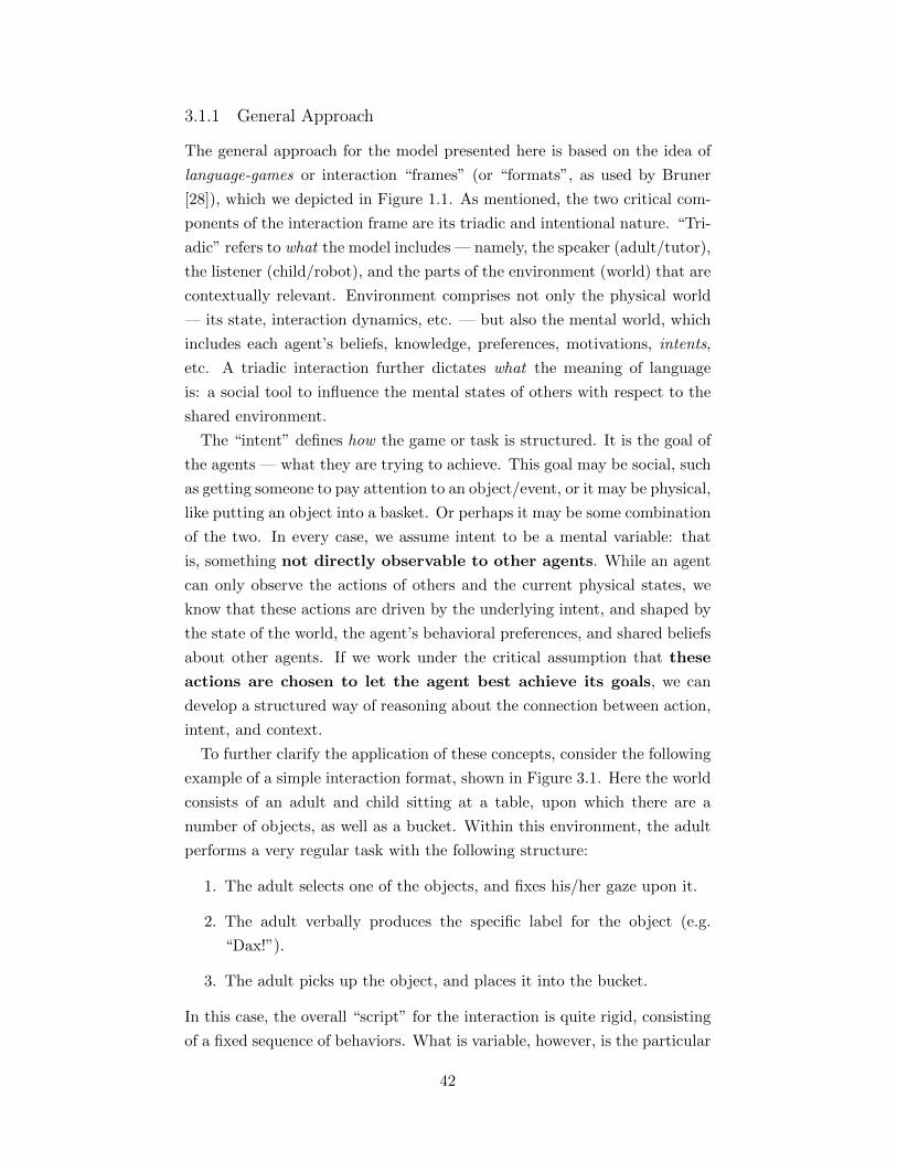
3.1.1 General Approach
The general approach for the model presented here is based on the idea of
language-games or interaction “frames” (or “formats”, as used by Bruner
[28]), which we depicted in Figure 1.1. As mentioned, the two critical com-
ponents of the interaction frame are its triadic and intentional nature. “Tri-
adic” refers to what the model includes — namely, the speaker (adult/tutor),
the listener (child/robot), and the parts of the environment (world) that are
contextually relevant. Environment comprises not only the physical world
— its state, interaction dynamics, etc. — but also the mental world, which
includes each agent’s beliefs, knowledge, preferences, motivations, intents,
etc. A triadic interaction further dictates what the meaning of language
is: a social tool to influence the mental states of others with respect to the
shared environment.
The “intent” defines how the game or task is structured. It is the goal of
the agents — what they are trying to achieve. This goal may be social, such
as getting someone to pay attention to an object/event, or it may be physical,
like putting an object into a basket. Or perhaps it may be some combination
of the two. In every case, we assume intent to be a mental variable: that
is, something not directly observable to other agents. While an agent
can only observe the actions of others and the current physical states, we
know that these actions are driven by the underlying intent, and shaped by
the state of the world, the agent’s behavioral preferences, and shared beliefs
about other agents. If we work under the critical assumption that these
actions are chosen to let the agent best achieve its goals, we can
develop a structured way of reasoning about the connection between action,
intent, and context.
To further clarify the application of these concepts, consider the following
example of a simple interaction format, shown in Figure 3.1. Here the world
consists of an adult and child sitting at a table, upon which there are a
number of objects, as well as a bucket. Within this environment, the adult
performs a very regular task with the following structure:
1. The adult selects one of the objects, and fixes his/her gaze upon it.
2. The adult verbally produces the specific label for the object (e.g.
“Dax!”).
3. The adult picks up the object, and places it into the bucket.
In this case, the overall “script” for the interaction is quite rigid, consisting
of a fixed sequence of behaviors. What is variable, however, is the particular
42
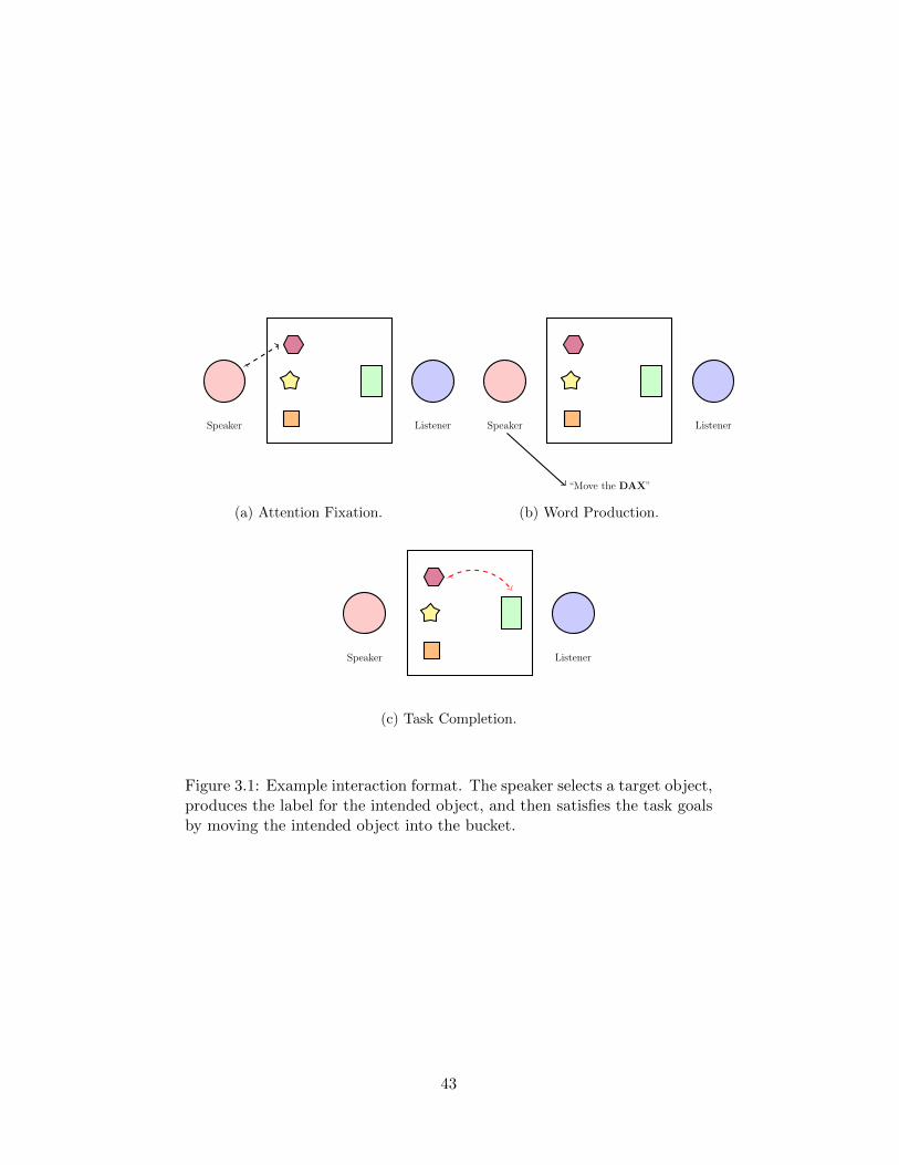
Speaker Listener
(a) Attention Fixation.
“Move the DAX”
Speaker Listener
(b) Word Production.
Speaker Listener
(c) Task Completion.
Figure 3.1: Example interaction format. The speaker selects a target object,produces the label for the intended object, and then satisfies the task goalsby moving the intended object into the bucket.
43
object that is selected, which will in turn affect the specifics of some of the
actions (i.e. particular reach position, word produced, etc.). By learning
about the general task structure, the child can learn about the connection
between a word label, and a specific intent — namely to place a specific
object in the bucket. This will be the general approach taken here: the
robot first learns about the intentional structure of a task, and then uses
this structure to learn the meanings of words.
3.1.2 Motivating Examples
In the previous example, there are multiple, redundant sources of informa-
tion the learner could use to determine intent: gaze, reaching for an object,
and moving it to the bucket. However, in many real-world interactions, a
child may have access to only one of these sources, which itself may be am-
biguous. As we have discussed, however, children often appear to be capable
of learning meanings of words by inferring the underlying intent of interac-
tion through a wide variety of other types of information. For the purposes
of practicality, we will focus on three simple means by which they appear to
do this, as demonstrated in the developmental literature.
Lexical Contrast
The first among these is often called “lexical contrast” [116], or under more
strict interpretations, “mutual exclusivity” [18]. In scenarios that attempt
to demonstrate and test this ability, the interaction format consists of a
child, an adult, and a number of toys/objects that are present in the envi-
ronment, some of which the child already knows the names of them. The
adult ambiguously attends to some set of objects, only one of which has
an unknown label, and then gives the label for the unknown object. Un-
der a pragmatic account, the child reasons that: “If the adult had meant
object X s/he would have used word A, so they must be using label B to
refer to object Y ”. In this most basic pragmatic reasoning, the listener is
able to constrain ambiguity by reasoning about how a speaker would act if
maximizing expected utility.
Goal-Directed Behaviors
It is also possible for a listener to infer intent from a speaker’s physical goal-
directed actions. In one study, an adult established an interaction format
44
with a child consisting of a finding-game where the adult gave the label for
the object s/he was intending to find, then pulled objects out of a bucket,
inspected them, and handed them over to the child [21]. Children were
shown to be able to learn the correct word-referent pairing, even in cases
where the adult inspected and rejected multiple objects before finding the
intended one. In another case, children were able to infer the correct intent
when the adult was unable to retrieve the objects altogether (i.e. the object
could not be removed from the bucket), given that they knew which objects
were in each bucket [20]. In both experiments, the child leveraged knowledge
about the interaction format in order to resolve ambiguity, even when goal-
directed actions were not completed, or were unsuccessful.
Action Constraints
The final set of experiments we will look at are those that appear to demon-
strate a child’s ability to reason about constraints on a speaker’s physical
actions, as well as his/her own (potential) role in the scenario, in order to
handle ambiguity [75, 24]. In these, an adult attempts to physically complete
some task — known to both the adult and the child — such as grabbing
a particular object and placing it in a specific location. When the adult
is able to grab certain objects and not others, the child interprets a verbal
request from the adult as a reference to an object, and is able to physically
aid the adult in completing his/her goal. The proposed explanation for the
child’s reasoning is that the adult would not have verbally referred to an
object they were capable of reaching themselves, so the unreachable object
must be the intent. While these particular experiments did not address word
learning directly, the pragmatic principles demonstrated are quite relevant
to this thesis.
3.1.3 Modeling Approach
The model and techniques presented in this section form the foundational
elements that will allow us to begin to move beyond many of the current lim-
itations of grounded language acquisition systems. They have been inspired
in large part by the growing body of research focusing on the links between
the comprehension and production of action and language [50, 117]. Work in
cognitive developmental robotics in particular has begun to develop general
computational frameworks for language processing and acquisition that fo-
cus on the kinds of intentional, pragmatic reasoning principles that can only
45
be achieved through embodied, situated, interaction [118, 62]. However, lit-
tle has been done in terms of creating detailed models and implementations
for these ideas, or figuring out how they can be applied to problems such as
language acquisition.
As we have just outlined, our approach in addressing this open issue will
be to focus on interactions involving both physical and communicative be-
haviors with a common underlying intentional structure, which are of critical
importance in a child’s linguistic development [27, 28]. At its foundation,
our model will be built around techniques for inverse planning, where ac-
tions are understood in terms of the goals or rewards they maximize. It
is these goals into which we embed our representation for the meaning of
words, and they are therefore a critical component to the methods we use.
Just as critical are the components that influence the ways in which ac-
tions are taken: beliefs about other agents, the world, and the interactions
between these three components.
We begin by using a basic signaling-game model to build a representation
of word meaning based on communicative utility, and derive a simple method
for online learning of this word-meaning mapping from training examples
featuring some amount of ambiguity. Following this, we extend the model
to the realm of physical action by embedding it within a Markov decision
process framework. We then provide a goal-based representation of the kinds
of interaction formats we have just described, and show how we can apply
techniques from inverse reinforcement learning [103, 102] to first acquire
knowledge about the general format of the interaction, and later to learn
words from ambiguous, yet goal-directed behaviors within the interaction.
In Section 3.4, we develop a truly triadic pragmatic word-learning engine
by unifying these two models through the agent’s understanding of its own
embodiment and role in the interaction. Finally, we show how our agent can
apply the same representations, and in service with its intentional inference
capabilities, take an active role in the interactions and its own learning.
3.2 Basic Pragmatic Model
For our first steps in the development of a basic pragmatic model for early
word learning, we focus on the core learning faculties of cross-situational
learning and lexical contrast, with the objective of later extending the model
to capture more complex behaviors. To do this we start from the game-
theoretic framework, and consider the very simple scenario where an adult
46
tutor produces a word describing an object s/he is attending to. Let us
also introduce basic referential ambiguity by allowing this attention to be
distributed over a confusion set of objects that contains the referent.
3.2.1 Mathematical Formulation
We begin by representing this scenario as an extensive-form game of incom-
plete information: the signaling game. However, as discussed in Section
2.3.3, traditional game-theoretic approaches of finding equilibria do not ap-
ply here. Instead, our approach is to first assume that the speaker σ and the
listener ρ are rational agents, who seek to maximize their expected utility.
Based only on her observation of the message, a ∈ A, the listener makes an
interpretation, d ∈ D, of the speaker’s intended referent, i ∈ I. The speaker
makes the decision about which a to send based on his belief about how the
listener will interpret the message. If the speaker is a rational agent, as we
assume, the relationship between their policy and beliefs can be expressed
as:
σ(i, a) = P (A = a|I = i) ∝ E [Uσ(i, d)|a] . (3.1)
E [Uσ(i, d)|a] =∑d∈D
P (D = d|A = a)Uσ(i, d). (3.2)
But what is the agent’s utility Uσ(i, d)? This is a question that is wrapped
up in the nature of intent itself, as it depends on the ability of the listener to
make an inference, d, that satisfies the speaker’s intent, i. For the scenario
discussed here, the intent is for the listener to attend to a particular object,
which we will assume they are able to do only if the correct inference is
made. Therefore, we let Uσ(i, d) = Uρ(i, d) be equal to 0 whenever i 6= d,
and some positive value R whenever i = d. From this we can write the
expectation of the speaker’s utility as
E [Uσ(i, d)|a] =∑d∈D
P (D = d|A = a)Uσ(i, d),
= P (D = i|A = a) ·R. (3.3)
As noted in Section 2.3.3, and as we can see from equation (3.2), a Bayesian
perfect equilibrium requires that the speaker hold some belief about how
the listener will respond. For now, we will define such a belief as ρ(a, d) =
47
P (D = d|A = a).
The listener is also assumed to be rational, governed by a policy favoring
moves that yield greater expected payoffs, similar to equation (3.1). How-
ever, the listener differs from the speaker in that s/he makes a decision after
having observed the speaker’s action a. The listener’s expected utility is
given by:
E [Uρ(i, d)|a, z] =∑i∈I
P (I = i|A = a, Z = z)Uρ(i, d). (3.4)
In equation (3.4), we introduce the variable Z to represent other information
the listener may use to shape their prior belief about the speaker’s intent.
In Sections 3.3 and 3.4, we will show how this can be done based on knowl-
edge of the task structure and/or physical actions of the speaker. For the
scenarios explored here, we consider simpler social cues, like gaze, as ways
of constraining the set of possible intended referents. Here, Z might let us
narrow down I to some subset of the entire set of objects present in the
scene, I = D = 1, 2, . . . No, which need not match the number of words
used in the scenario in size (i.e. |A| 6= No).
We use the third condition for a perfect Bayesian equilibrium (PBE) —
belief consistency — to calculate the posterior probability P (I|A,Z), the
probability of a speaker’s intent given information about his/her possible
focus of attention, Z, and their use of message A. First we apply Bayes’
theorem:
P (I|A,Z) =P (A|I, Z)P (I|Z)∑
i′P (A|I = i′, Z)P (I = i′|Z)
, (3.5)
to yield an expression in terms of P (A|I, Z) and P (I|Z). The prior P (I|Z)
is analogous to those used in previously discussed game-theoretic models of
pragmatics. The conditional probability P (A|I, Z) is the probability that
the speaker will use message A given intent I. We make the simplifying
assumption that the message and the speaker’s attentional state are inde-
pendent given intent, P (A|I, Z) = P (A|I), which makes this an estimate of
the stochastic policy of the speaker.
Calculation of this posterior distribution requires a belief about the speaker’s
strategy P (A|I). We have already discussed in our brief review of game the-
ory how common signaling game approaches of equilibrium selection do not
apply well to a child learner. Alternatively, we have pointed out that the
game-theoretic learning approach of choice — reinforcement learning — does
not match the actual conditions of child learners who often learn without
48
any kind of explicit feedback or unequivocal knowledge of correct referent.
So how can we begin to learn about the speaker’s linguistic strategy us-
ing only knowledge of the message, and some additional information on the
intent prior P (I|Z)?
For our approach we assume that the listener, to the extent that s/he
can, still plays in line with PBE. The first way we do this is by having the
listener choose interpretations d for each interaction episode that maximize
expected payoff given a posterior belief calculated by equation (3.5). The
second way is by allowing the listener to understand that the speaker is a
rational agent given his/her beliefs about the listener’s response policy. In
Section 3.2.1, we used equation (2.33) to note that the speaker’s policy (and
the receiver’s belief about it), had only the requirement that it maximize the
speaker’s expected utility. This idea can be approximated in a probabilistic
setting like the one here, by using a softmax function to define a stochastic
policy of the speaker that depends on his expected utility:
P (A = a|I = i) = σ(i, a) =eαE[Uσ(i,a)]∑
a′eαE[Uσ(i,a′)]
. (3.6)
While the listener now knows how to make an interpretation for some given
observations, a and z, they are still faced with the problem of learning a
model for the speaker’s strategy σ(i, a).
3.2.2 Learning Algorithm
Under equations (3.6) and (3.2), the problem for the listener is not so much
the direct learning of the speaker’s policy as it is the learning about the
speaker’s beliefs on the listener’s own policy ρ(a, d). We would like the
listener to gradually bring his/her own beliefs about their response policy
ρ(a, d) in line with the speaker’s “prescribed” policy. A number of differ-
ent approaches exist for solving this task. As this is essentially a hidden
variable model, one way might be to apply EM-type algorithms to learn
a parameterized approximation of the policy, similar to many of the pop-
ular association-based models discussed earlier [4]. However, such batch
learning algorithms ignore the incremental and dynamic nature of language
acquisition in real language learners that is essential in faithfully capturing
phenomena like lexical contrast.
Instead, our initial attempts at approaching this problem will be based on
a stochastic gradient descent approach. Here, we use a maximum-likelihood
objective function, which offers us a way to estimate the stochastic policy
49
model used by the speaker based only on the observed data that was gen-
erated using the model. Recall that stochastic gradient descent techniques
for MLE optimize the log-likelihood function by updating the parameter set
each time an observation is taken, as shown in equation (2.4).
To apply this method to our problem, we first define the model as a
function of parameter vector φ ∈ R|A|×|I|, so that each φj,k is equal to
the probability that the listener chooses interpretation D = k after hearing
message A = j:
φj,k , P (D = k|A = j), (3.7)∑k
φj,k = 1. (3.8)
Next, we derive the likelihood function of a single observation, at time
t. Because the observations are dependent on a hidden variable I — the
speaker’s intent — the likelihood function takes the form:
P (at|zt, φ) =∑i
P (i, at|zt, φ)
=∑i
σ(i, at;φ)P (i|zt), (3.9)
where the function σ(i, a, φ) is the parameterized version of the listener’s
estimate of the speaker’s stochastic policy originally given in equation (3.6).
After each observation sample (at, zt), each parameter φj,k in the vector is
updated by moving along its gradient of the log-likelihood function:
∂
∂φj,klog [P (at|zt, φ)] =
∂
∂φj,klog
[∑i
σ(i, at;φ)P (i|zt)
]
=1∑
iσ(i, at;φ)P (i|zt)
·
[∑i
P (i|zt) ·∂
∂φj,kσ(i, at;φ)
]. (3.10)
Finding the gradient involves finding the partial derivative of the softmax
function, which fortunately produces a very simple closed form expression.
First, let us define the indicator function I(x, y) as having value 1 when
its two arguments are equal, and 0 otherwise. Derivatives of the speaker’s
50
stochastic policy with respect to parameter φj,k are given by:
∂
∂φj,kσ(i, at;φ) = ασI(k, i) · σ(i, at;φ) [I(j, at)− σ(i, j;φ)] . (3.11)
Recall that in this parameterization the individual parameters correspond
to stochastic response policies of the listener, requiring the constraint that
the sum of all φj,ks for a single k must be equal to 1. After each update
step, the parameter vector is projected back onto the allowable probability
manifold specified by this constraint. This projection operation is denoted
by ΠG, and is performed using the algorithm described in [40].
3.2.3 Discussion
The purpose of the material presented in this section was twofold. The first
objective was to create a model capable of representing the associations be-
tween words and their meanings, and to derive an algorithm for incremen-
tally learning these associations from potentially ambiguous observations.
The second objective was for the model to be capable of demonstrating
the emergence of so-called “lexical contrast” (or more strictly, mutual ex-
clusivity) biases observed in child word learners[18] from basic pragmatic
principles.
Our intuition about how this emerges comes from the model’s understand-
ing of a word in terms of the goal it is trying to achieve, as exemplified in
equations (3.5) and (3.6). Consider the case where our learner is presented
with a novel word label, a′, and an ambiguous set of possible referent ob-
jects, many or most of which are already known to have other labels. In
making its inference of the posterior probability, P (I|A,Z, φ), our agent rea-
sons about the probability that the speaker would have used the new label,
given each hypothesis about the intent. For objects with known words, the
novel referent would likely not be as effective in getting the listener to rec-
ognize the intended referent. Therefore, P (a′|I, φ) (equation 3.6) would be
low for such objects, while it might be close to chance for objects without
known labels, ultimately resulting in a posterior probability that favored
this later set of objects. It is in this way that the lexical contrast reasoning
is captured by the basic model’s general pragmatic understanding of word
use. In Section 3.3, we will see how these same kinds of principles can be
applied to learning and reasoning about physical goal-directed behaviors.
51
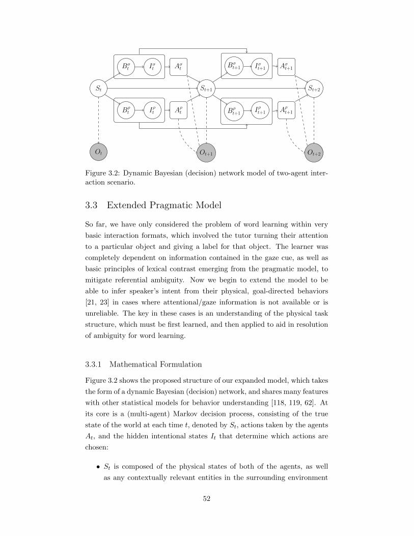
St
Ot
Bσt Iσt Aσ
t
Bρt Iρt Aρ
t
St+1
Ot+1
Bσt+1 Iσt+1 Aσ
t+1
Bρt+1
Iρt+1 Aρt+1
St+2
Ot+2
Figure 3.2: Dynamic Bayesian (decision) network model of two-agent inter-action scenario.
3.3 Extended Pragmatic Model
So far, we have only considered the problem of word learning within very
basic interaction formats, which involved the tutor turning their attention
to a particular object and giving a label for that object. The learner was
completely dependent on information contained in the gaze cue, as well as
basic principles of lexical contrast emerging from the pragmatic model, to
mitigate referential ambiguity. Now we begin to extend the model to be
able to infer speaker’s intent from their physical, goal-directed behaviors
[21, 23] in cases where attentional/gaze information is not available or is
unreliable. The key in these cases is an understanding of the physical task
structure, which must be first learned, and then applied to aid in resolution
of ambiguity for word learning.
3.3.1 Mathematical Formulation
Figure 3.2 shows the proposed structure of our expanded model, which takes
the form of a dynamic Bayesian (decision) network, and shares many features
with other statistical models for behavior understanding [118, 119, 62]. At
its core is a (multi-agent) Markov decision process, consisting of the true
state of the world at each time t, denoted by St, actions taken by the agents
At, and the hidden intentional states It that determine which actions are
chosen:
• St is composed of the physical states of both of the agents, as well
as any contextually relevant entities in the surrounding environment
52
(e.g. objects).
• At are the actions available to each agent. These may be physical
(e.g. moving one’s arm to push an object) or communicative (e.g. an
utterance like “Dax!”) in nature.
• It represents what the agent is trying to accomplish through its actions.
It may be to realize a particular physical state, mental state of an
agent, or both (e.g. to have a listener attend to the pushing of a
particular object).
Two other important elements of the model are the “Belief” states of the
agents, Bt, and the observations Ot. Bt encodes the beliefs or knowledge
of an agent about the aspects of the interaction that are not its specific
intent, such as the current state of the world (which we assume to be per-
fectly known here), the knowledge about the goal structure of the current
interaction/task, or expected linguistic conventions (i.e. ρ and the listener’s
accompanying estimate of φ in Section 3.2). Because the mental states
(intents, beliefs) and actions we have described are not necessarily shared
between the agents, we use the superscripts σ and ρ to denote those variables
as they pertain to the speaker and listener, respectively.
For completeness, we also include Ot for cases where the true state of
the world and actions can only be inferred from noisy sensor observations.
This aspect will become more critical in later sections, as we focus on the
issues of perception that come with real-world, embodied implementations.
For the sake of the current discussion, we will assume to work with directly
observable states and actions.
Another piece that is critical for defining this model, as with the MDP
upon which it is built, are the physical transition dynamics. These are
represented as a distribution P (St+1|St, At) over the state of the world in
the next time step, conditioned on the current state and actions of the
agents. As with our discussion on MDPs in Chapter 2, we use the notation
T (s, s′, a) to refer to the probability of a specific state-action-state transition.
This model can capture the effects that various actions will produce in the
environment, as well as the uncertainty of these effects. Practically, it can
also be used to encode physical constraints and limitations on agents.
Generating Actions, Inferring Intent
We now come to the problem of how this extended model can be applied
to provide our learner with the desired capability to resolve referential am-
53
biguity by understanding the speaker’s physical, goal-directed behaviors.
We begin by defining the state and action spaces that will be necessary to
represent the critical features of the interaction scenarios discussed at the
beginning of this chapter. Our representation of the state space will clearly
be dependent on the particular scenario for each of these, but in general it
encompasses the states of the speaker/tutor, listener/learner, and any ob-
jects present in their shared environment. We will assume that our agent
knows the state can be described as a factored representation, consisting of
the set of states for these individual elements. Therefore, we can express
the state St as a vector variable over these states, drawn over a domain S,
that is the Cartesian product of the state spaces for the individual elements
and entities:
St =(Sσt , S
ρt , S
o,1t , . . . So,Not
), (3.12)
S = Sσ × Sρ × So,1 × . . .So,No , (3.13)
where So,n refers to the state space of the n-th object out of No in the
environment. For the experimental scenarios discussed in this thesis, we will
primarily use the spatial location of the objects, or in the case of the agents,
the end-effector, as the information encoded within the states. Specific
details of how these states are defined and determined from the robot’s
perceptual capabilities will be discussed in Chapter 5.
As we mentioned previously, there are two types of actions that we wish
to represent within this framework: physical and communicative, which we
treat as two disjoint sets. Physical actions, like the state space, will involve
both of the agents and the objects within the environment. Unlike the state
space, however, there are two separate action spaces for the speaker and lis-
tener. Rather than representing an agent’s actions as the movement of their
end-effectors and creating a complex model of how these physical interact
with various objects, we consider the action space to be the movements of
the objects themselves. Assuming that the agent can only effect movement
on one object at a time, we define physical actions to be an element of the
union of the action sets for individual objects:
54
Ap = Ao,1⋃. . .Ao,No , (3.14a)
Aσp ⊆ Ap, (3.14b)
Aρp ⊆ Ap. (3.14c)
The set of actions for each of the agents is some subset of the complete
actions over these objects, and they need not be equal to one another. In
our implementation (detailed in Chapter 5) we will generally treat individ-
ual action spaces as movements in the four cardinal directions, plus a “no-
movement” action. As done in the basic pragmatic model, we assume the
set of communicative actions to be single word symbols, which we denote as
Am = 1, 2, . . .M. In the service of brevity in the following discussion, spe-
cific communicative actions will be identified as m ∈ Am, while unspecified
actions, a, are assumed to refer to physical actions.
We now return to the problem of word learning. In the scenarios motivat-
ing this stage of model development, the objective was to use observations
of an agent’s goal-directed action to aid in resolving ambiguity during word
learning, under the premise that both the communicative and physical ac-
tion of the adult were driven by some underlying intent. For the sake of
simplicity, let all unlabeled intents and actions in the following section re-
fer to those of the speaker (At = Aσt , It = Iσt ) unless otherwise specified.
Suppose that in a single episode of the new word-learning scenario, our
agent observes the speaker taking some communicative action m ∈ Am, as
well as an accompanying physical action, in the form of a state-action se-
quence, st, atTt=0. Let us also assume that for all t over the course of this
training episode, the speaker’s intent It does not change. We now rewrite
the likelihood objective function of equation (3.9) to include the additional
information about the speaker’s goal-directed actions:
P (m|st, atTt=0, φ) =∑i
P (i,m|st, atTt=0, φ)
=∑i
P (m|i, φ)P (i|st, atTt=0). (3.15)
As before, our intuition is that we can exploit contextual information in
order to reduce ambiguity in the inference of intent. Under our framework
of (sequential) rational action, we can calculate the posterior over intentions
using the same kind of softmax calculation of action probabilities (as in equa-
55
tion (2.26)) that was used in Chapter 2’s discussion of inverse reinforcement
learning:
P (i|st, atTt=0) ∝ P (st, atTt=0|i), (3.16)
P (st, atTt=0|i) =
T∏t=0
P (st, at|i), (3.17)
P (a|s, i) =eαQ
∗i (s,a)∑
a′eαQ
∗i (s,a′)
, (3.18)
where Q∗i (s, a) is the optimal Q-function under intent i, as given in equa-
tion (2.19). Equations (3.17) and (3.18) give the probability that a spe-
cific reward function would have produced the speaker’s observed behavior,
which we intuitively understand to be dependent on our speaker’s intent.
This leaves us with the significant challenge of how to define intent, and
more specifically, how it is to be used to parameterize Ri (and consequently
Q∗i (s, a)).
In our basic model, the purpose of utterances was for the listener to rec-
ognize and share attention to an intentional state that was simply one of
the objects present in the environment. For these extended scenarios, how-
ever, the intent consists not only of the objects themselves, but also the
target state of each of the objects that the speaker wishes to affect through
physical action. In such cases, simple object labels alone are not sufficient
to generate a reward function R ∈ R|S| needed to represent such an intent.
At the same time, allowing the space of intents to span the combined state
space defined in equation (3.13) would make little sense as a representation
of word meaning, and it certainly would not be a computationally feasible
inference problem.
This is where the key idea of the structured interaction format or task
comes into play. For many of the situations in which children learn their
first words, there is often some very regular task being performed, which
varies in only some small aspect, such as the object(s) upon which it is
being performed, as in the motivating examples for this section [20, 21].
This allows the learner to greatly constrain the space of intents (or reward
functions) over which the inference takes place. Furthermore, knowledge
acquired about regularities of the task being performed can be used by the
listener to learn word meanings for the variable aspects of the format, even
when performance of the task is incomplete or unsuccessful.
Even under the relatively narrow state and action spaces we have proposed
56
here, creating models capable of the autonomous construction and learning
of representations for complex interactions and their mapping into linguistic
structures would be an immensely difficult task. For the purposes of our
experiment, we assume knowledge of the variable elements of the
task to be some set of objects, which implicitly defines, as well as limits,
our representation of word meanings.
Under this key assumption, we now define the space of intents as I ∈1, 2, . . . N, just as before. But even if we assume to know what reduced
representation of the task space is relevant for the given word, we still need to
determine its relationship to knowledge about the task being performed, how
this task knowledge is represented, and finally how these are used to generate
the reward representation needed for effective application of equation (3.18).
For this purpose, we present the following function for generating rewards
based on the specific intent, and knowledge about the physical task of the
interaction:
Ri(s; θ) = θTψ(gi(s)). (3.19)
The reward function for each intent is generated according to a linear “feature-
based” formula, similar to the one given in equation (2.10). It consists of
the following components:
• gi : S → S: This function selects a subset Si ⊆ S of the state-space
specific to intent i.
• ψ : S → Rf : This function generates a set of features for each state in
the reduced, intent-specific state space.
• θ ∈ Rf : The column vector of reward weights for each feature. This
represents the invariant aspects of the interaction task.
An example of gi might be to simply select the state variable(s) correspond-
ing to the particular object i: gi(St) = So,it . Whatever the implementation,
it is important that the domain of state variables be identical for all Si. This
allows the feature function ψ and task parameter θ to represent the aspects
of the goal/reward function that are invariant across intended objects.
We use this representation of the reward function to define the intent-
dependent optimal Q-function Q∗i (s, a; θ) given task parameter θ:
57
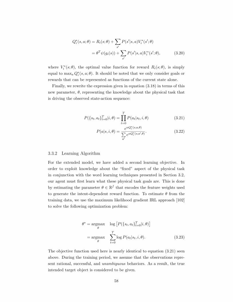
Q∗i (s, a; θ) = Ri(s; θ) +∑s′
P (s′|s, a)V ∗i (s′; θ)
= θTψ(gi(s)) +∑s′
P (s′|s, a)V ∗i (s′; θ), (3.20)
where V ∗i (s; θ), the optimal value function for reward Ri(s; θ), is simply
equal to maxaQ∗i (s, a; θ). It should be noted that we only consider goals or
rewards that can be represented as functions of the current state alone.
Finally, we rewrite the expression given in equation (3.18) in terms of this
new parameter, θ, representing the knowledge about the physical task that
is driving the observed state-action sequence:
P (st, atTt=0|i, θ) =T∏t=0
P (at|st, i, θ) (3.21)
P (a|s, i, θ) =eαQ
∗i (s,a,θ)∑
a′eαQ
∗i (s,a′,θ)
. (3.22)
3.3.2 Learning Algorithm
For the extended model, we have added a second learning objective. In
order to exploit knowledge about the “fixed” aspect of the physical task
in conjunction with the word learning techniques presented in Section 3.2,
our agent must first learn what these physical task goals are. This is done
by estimating the parameter θ ∈ Rf that encodes the feature weights used
to generate the intent-dependent reward function. To estimate θ from the
training data, we use the maximum likelihood gradient IRL approach [102]
to solve the following optimization problem:
θ∗ = argmaxθ
log[P (st, atTt=0|i, θ)
]= argmax
θ
T∑t=0
logP (at|st, i, θ). (3.23)
The objective function used here is nearly identical to equation (3.21) seen
above. During the training period, we assume that the observations repre-
sent rational, successful, and unambiguous behaviors. As a result, the true
intended target object is considered to be given.
58
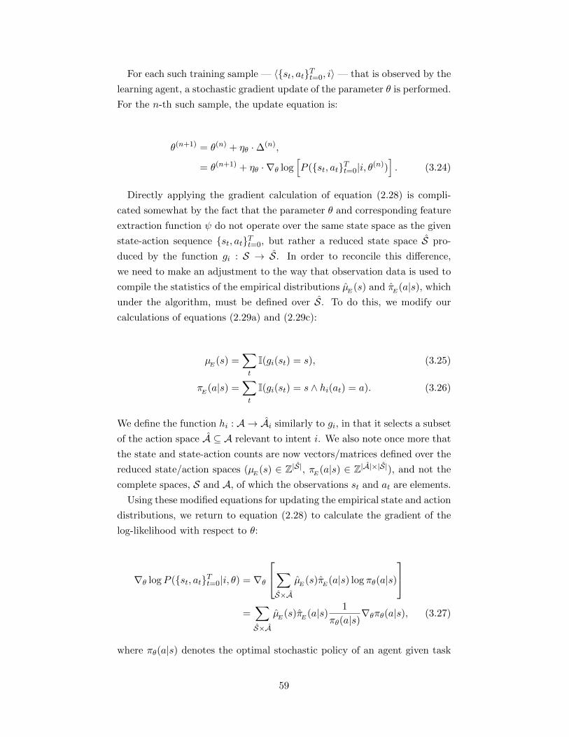
For each such training sample — 〈st, atTt=0, i〉— that is observed by the
learning agent, a stochastic gradient update of the parameter θ is performed.
For the n-th such sample, the update equation is:
θ(n+1) = θ(n) + ηθ ·∆(n),
= θ(n+1) + ηθ · ∇θ log[P (st, atTt=0|i, θ(n))
]. (3.24)
Directly applying the gradient calculation of equation (2.28) is compli-
cated somewhat by the fact that the parameter θ and corresponding feature
extraction function ψ do not operate over the same state space as the given
state-action sequence st, atTt=0, but rather a reduced state space S pro-
duced by the function gi : S → S. In order to reconcile this difference,
we need to make an adjustment to the way that observation data is used to
compile the statistics of the empirical distributions µE (s) and πE (a|s), which
under the algorithm, must be defined over S. To do this, we modify our
calculations of equations (2.29a) and (2.29c):
µE (s) =∑t
I(gi(st) = s), (3.25)
πE (a|s) =∑t
I(gi(st) = s ∧ hi(at) = a). (3.26)
We define the function hi : A → Ai similarly to gi, in that it selects a subset
of the action space A ⊆ A relevant to intent i. We also note once more that
the state and state-action counts are now vectors/matrices defined over the
reduced state/action spaces (µE (s) ∈ Z|S|, πE (a|s) ∈ Z|A|×|S|), and not the
complete spaces, S and A, of which the observations st and at are elements.
Using these modified equations for updating the empirical state and action
distributions, we return to equation (2.28) to calculate the gradient of the
log-likelihood with respect to θ:
∇θ logP (st, atTt=0|i, θ) = ∇θ
∑S×A
µE (s)πE (a|s) log πθ(a|s)
=∑S×A
µE (s)πE (a|s) 1
πθ(a|s)∇θπθ(a|s), (3.27)
where πθ(a|s) denotes the optimal stochastic policy of an agent given task
59
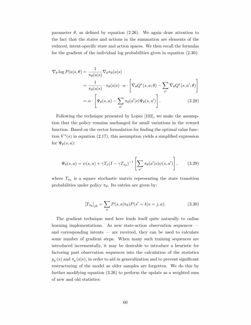
parameter θ, as defined by equation (2.26). We again draw attention to
the fact that the states and actions in the summation are elements of the
reduced, intent-specific state and action spaces. We then recall the formulas
for the gradient of the individual log probabilities given in equation (2.30):
∇θ logP (a|s, θ) =1
πθ(a|s)∇θπθ(a|s)
=1
πθ(a|s)· πθ(a|s) · α ·
[∇θQ∗(s, a; θ)−
∑a′
∇θQ∗(s, a′; θ)
]
= α ·
[Ψθ(s, a)−
∑a′
πθ(a′|s)Ψθ(s, a
′)
]. (3.28)
Following the technique presented by Lopes [102], we make the assump-
tion that the policy remains unchanged for small variations in the reward
function. Based on the vector formulation for finding the optimal value func-
tion V ∗(s) in equation (2.17), this assumption yields a simplified expression
for Ψθ(s, a):
Ψθ(s, a) = ψ(s, a) + γTa(I − γTπθ)−1
[∑a′
πθ(a′|s)ψ(s, a′)
], (3.29)
where Tπθ is a square stochastic matrix representing the state transition
probabilities under policy πθ. Its entries are given by:
[Tπθ ]jk =∑a
P (s, a|πθ)P (s′ = k|s = j, a). (3.30)
The gradient technique used here lends itself quite naturally to online
learning implementations. As new state-action observation sequences —
and corresponding intents — are received, they can be used to calculate
some number of gradient steps. When many such training sequences are
introduced incrementally, it may be desirable to introduce a heuristic for
factoring past observation sequences into the calculation of the statistics
µE (s) and πE (a|s), in order to aid in generalization and to prevent significant
restructuring of the model as older samples are forgotten. We do this by
further modifying equation (3.26) to perform the update as a weighted sum
of new and old statistics:
60
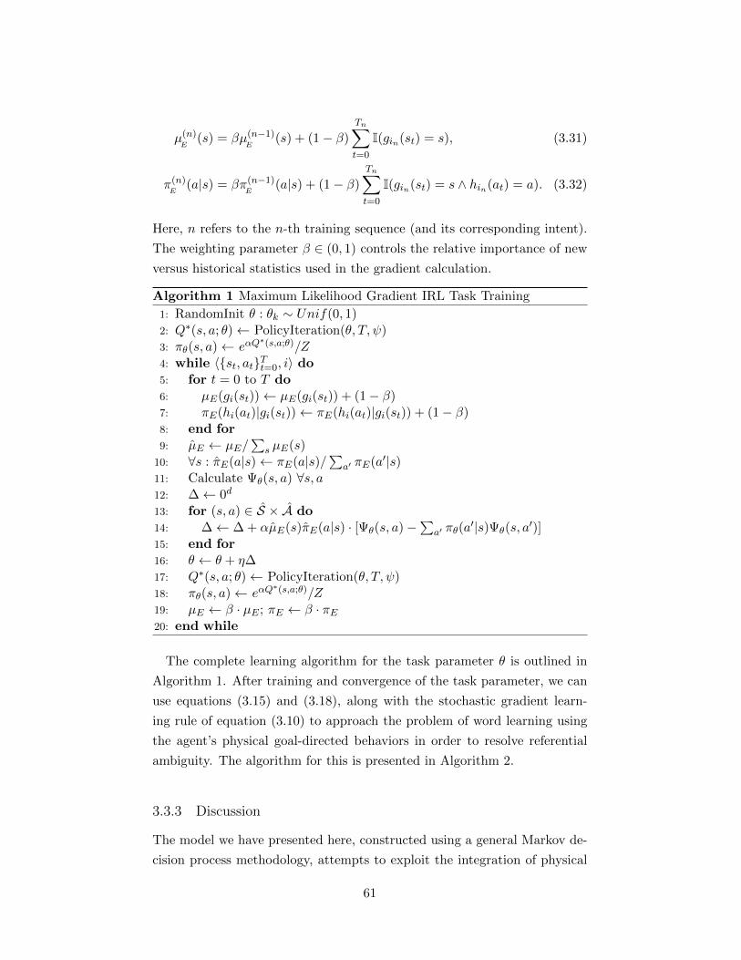
µ(n)E
(s) = βµ(n−1)E
(s) + (1− β)
Tn∑t=0
I(gin(st) = s), (3.31)
π(n)E
(a|s) = βπ(n−1)E
(a|s) + (1− β)
Tn∑t=0
I(gin(st) = s ∧ hin(at) = a). (3.32)
Here, n refers to the n-th training sequence (and its corresponding intent).
The weighting parameter β ∈ (0, 1) controls the relative importance of new
versus historical statistics used in the gradient calculation.
Algorithm 1 Maximum Likelihood Gradient IRL Task Training
1: RandomInit θ : θk ∼ Unif(0, 1)2: Q∗(s, a; θ)← PolicyIteration(θ, T, ψ)3: πθ(s, a)← eαQ
∗(s,a;θ)/Z4: while 〈st, atTt=0, i〉 do5: for t = 0 to T do6: µE(gi(st))← µE(gi(st)) + (1− β)7: πE(hi(at)|gi(st))← πE(hi(at)|gi(st)) + (1− β)8: end for9: µE ← µE/
∑s µE(s)
10: ∀s : πE(a|s)← πE(a|s)/∑
a′ πE(a′|s)11: Calculate Ψθ(s, a) ∀s, a12: ∆← 0d
13: for (s, a) ∈ S × A do14: ∆← ∆ + αµE(s)πE(a|s) · [Ψθ(s, a)−
∑a′ πθ(a
′|s)Ψθ(s, a′)]
15: end for16: θ ← θ + η∆17: Q∗(s, a; θ)← PolicyIteration(θ, T, ψ)18: πθ(s, a)← eαQ
∗(s,a;θ)/Z19: µE ← β · µE ; πE ← β · πE20: end while
The complete learning algorithm for the task parameter θ is outlined in
Algorithm 1. After training and convergence of the task parameter, we can
use equations (3.15) and (3.18), along with the stochastic gradient learn-
ing rule of equation (3.10) to approach the problem of word learning using
the agent’s physical goal-directed behaviors in order to resolve referential
ambiguity. The algorithm for this is presented in Algorithm 2.
3.3.3 Discussion
The model we have presented here, constructed using a general Markov de-
cision process methodology, attempts to exploit the integration of physical
61
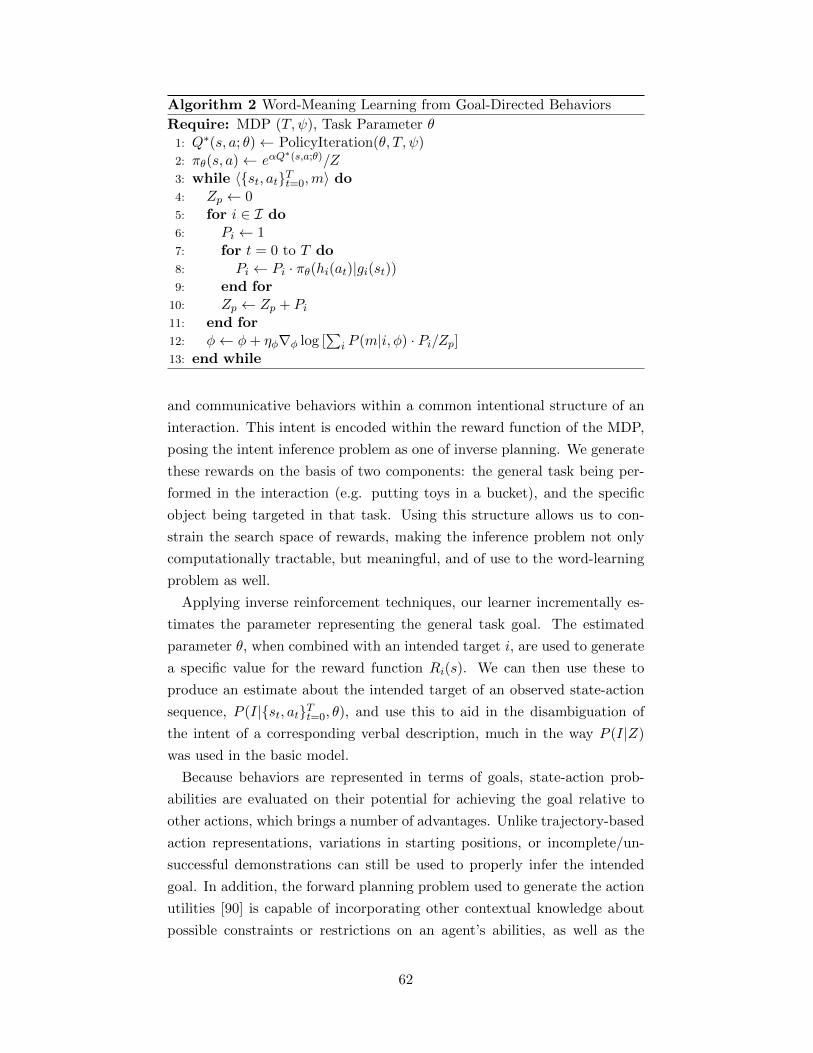
Algorithm 2 Word-Meaning Learning from Goal-Directed Behaviors
Require: MDP (T, ψ), Task Parameter θ1: Q∗(s, a; θ)← PolicyIteration(θ, T, ψ)2: πθ(s, a)← eαQ
∗(s,a;θ)/Z3: while 〈st, atTt=0,m〉 do4: Zp ← 05: for i ∈ I do6: Pi ← 17: for t = 0 to T do8: Pi ← Pi · πθ(hi(at)|gi(st))9: end for
10: Zp ← Zp + Pi11: end for12: φ← φ+ ηφ∇φ log [
∑i P (m|i, φ) · Pi/Zp]
13: end while
and communicative behaviors within a common intentional structure of an
interaction. This intent is encoded within the reward function of the MDP,
posing the intent inference problem as one of inverse planning. We generate
these rewards on the basis of two components: the general task being per-
formed in the interaction (e.g. putting toys in a bucket), and the specific
object being targeted in that task. Using this structure allows us to con-
strain the search space of rewards, making the inference problem not only
computationally tractable, but meaningful, and of use to the word-learning
problem as well.
Applying inverse reinforcement techniques, our learner incrementally es-
timates the parameter representing the general task goal. The estimated
parameter θ, when combined with an intended target i, are used to generate
a specific value for the reward function Ri(s). We can then use these to
produce an estimate about the intended target of an observed state-action
sequence, P (I|st, atTt=0, θ), and use this to aid in the disambiguation of
the intent of a corresponding verbal description, much in the way P (I|Z)
was used in the basic model.
Because behaviors are represented in terms of goals, state-action prob-
abilities are evaluated on their potential for achieving the goal relative to
other actions, which brings a number of advantages. Unlike trajectory-based
action representations, variations in starting positions, or incomplete/un-
successful demonstrations can still be used to properly infer the intended
goal. In addition, the forward planning problem used to generate the action
utilities [90] is capable of incorporating other contextual knowledge about
possible constraints or restrictions on an agent’s abilities, as well as the
62
abilities of other agents, which we will explore in Section 3.4.
3.4 Triadic Pragmatic Model
In this section, we show how the extended model can be developed even
further to reason pragmatically about a speaker’s intent based on knowledge
of their physical action constraints, as well as the listener’s own role in the
interaction [75, 24]. This is achieved not by adding new elements or layers of
complexity to the model, but rather by a more general treatment of language,
action, and the function of communication. In addition to its application
to the proposed experiments, we also show how it can be used to give the
agent a more interactive role in its own learning process.
3.4.1 Mathematical Formulation
In our presentation of both the basic and extended pragmatic models, we
have operated under the key assumption that the utility of an utter-
ance depends solely on correct interpretation by the listener. This
implicitly fixed a word’s pragmatic function as entirely referential, and as
a result, physical action and communicative action were effectively decou-
pled, though complementary. Intents had a “dual” nature: producing or
achieving some particular event or state (i.e. the physical aspect), and shar-
ing attention with the listener to this reference event/state/object (i.e. the
communicative aspect). These intents were fundamentally the same, but
they were inferred from mostly independent models and observations.
However, one thing that was the same for both physical and communica-
tive intention inferences, was their basis in the principle of utility maximiza-
tion. Each contained at its core the following calculation used to evaluate
the likelihood of seeing a particular action given an intentional state:
P ( A | I, Model ) =eα·E[ Utility (A) | I, Model ]∑
A′eα·E[ Utility (A′) | I, Model ]
. (3.33)
In Section 3.3, we employed an expected utility function ubiquitous in se-
quential planning problems, the Q-function. A function of both the current
state and action, and dependent on a given (optimal) action policy or strat-
egy, we know that Q∗(s, a) is equal to the immediate reward for the given
state-action, plus the expected value of the (discounted) future rewards re-
63
sulting from the state-action and given (optimal) policy. Assuming rewards
to be only dependent on the state, as we have done thus far, we can ex-
press the intent-dependent, task-parameterized Q∗i (s, a; θ) in a way similar
to equation (3.20):
Q∗i (s, a; θ) = Ri(s; θ) + γ∑s′
P (s′|s, a)V ∗i (s′; θ), (3.34)
= θTψ(gi(s)) + γ∑s′
P (s′|s, a)V ∗i (s′; θ), (3.35)
where the optimal value function V ∗i (s; θ) is simply equal to Q∗i (s, π∗(s); θ).
For communication, we likewise based the probability in part on an ex-
pectation of the utility/value over the state resulting from the action, shown
in equation (3.2). The only difference between this expression and equation
(3.35) is that the utility of an action is taken as an expectation over in-
fluenced mental states (i.e. inferred intentions) rather than physical ones.
Assuming that communication does not affect the physical state of the world
S, we might express this utility as a Q-function over communicative actions
am ∈ Am:
Q∗i (s, am; θ, φ) = Ri(s; θ) +∑d
P (D = d|s, am, φ)V ∗i (s, d; θ). (3.36)
Here, we have simply and naively augmented the value function in equation
(3.35) to include the listener’s interpretive state in addition to the physical
state s: V ∗i (s, d; θ). We recall from equation (3.3) that in our basic pragmatic
model, this function would have been defined as some positive constant
(R = 1 without loss of generality) if and only if i = d, and 0 otherwise.
Consider now the motivating experiments for this current section. In these
scenarios, the function of the speaker’s utterance goes beyond reference to
an object, and in fact constitutes a request for the object. The intent behind
the utterance can not be satisfied simply by proper comprehension alone,
but also requires some behavioral aid that perhaps only the listener can
provide. At the same time, because communication is being used in service
of some larger task goal, its expected utility is balanced against physical
means of completing the goal when planning actions. This planning task of
the speaker, and corresponding inference task of the listener, require each
to be able to leverage knowledge about the physical and communicative
abilities of both.
64
Before showing how our model can be used to do this, we define some
useful notations:
• Let πσ and πρ denote policies for the speaker and listener respectively.
πσ : S → Aσ and πρ : S → Aρ, where the action spaces are those
available to the speaker and listener respectively.
• Let πσ∗i (s; θ) denote the speaker’s optimal policy under reward Ri(s; θ)
for intent i and task parameter θ as defined in equation (3.19). Let
πρ∗i (s; θ) denote the same for the listener.
• Let V σ∗i (s; θ) refer to the value function at state s under intent i
and task parameters θ, under a speaker following the optimal policy
πσ∗i (s; θ) above.
• Let V ρ∗i (s; θ) be the same for the listener.
Each of the quantities defined here is already supported by the existing
framework of extended pragmatic model presented in Figure 3.2. And fol-
lowing from our discussion in the paragraphs above, the deep and intuitive
link between the planning (or understanding) of physical and communicative
actions allows us to achieve our goals through the generalization of existing
mathematical formulas rather than through the addition of more rules.
Returning to the case of a speaker’s request for the listener’s physical
help in completing a desired task with a particular object, we assume that
our cooperative listener will act optimally based on its interpretation of
the speaker’s intent, d, and knowledge of the task θ. Within our MDP
framework, we could also say that the listener acts according to the optimal
policy (over its own action space Aρ) for reward Rd(s; θ): πρ∗d (s; θ). While
this reward drives the listener’s actions, it is not necessarily the same reward
Ri(s; θ) used to calculate the augmented value function V ∗i (s, d; θ).
Rather than evaluate the value function for every possible combination of
i and d, we assume that V ∗i (s, d; θ) = 0 for all i 6= d. Note the difference
between this assumption, and the similar but much stricter definition on
the utility made in the basic model. This assumption in effect disregards
any possibility that the listener might “accidentally” achieve goal i during
its attempted pursuit of goal d. As a result, the expected value in equation
(3.36) becomes equal to the probability that the correct interpretation is
made, times the value the listener can provide in completing that specific
task.
65
In order to evaluate the intent of a speaker given their goal directed ac-
tions, we use the softmax calculation of the action probabilities from ex-
pected utilities, given in equation (3.33), once more:
P (a|s, i, θ, φ) =eαQ
∗i (s,a;θ,φ)∑
a′eαQ
∗i (s,a′;θ,φ)
. (3.37)
We define a unified utility function for the speaker Q∗i (s, a; θ, φ) thusly:
Q∗i (s, a; θ, φ) =
Ri(s; θ) + γ
∑s′P (s′|s, a)V σ∗
i (s′; θ) if a ∈ Ap
Ri(s; θ) + P (D = i|s, a, φ)V ρ∗i (s; θ) if a ∈ Am
, (3.38)
where Ap and Am refer to the sets of physical and communicative (i.e.
words) actions available to the speaker. This expression is essentially a
unification of equations (3.35) and (3.36), with a more explicit definition
for V ∗i (s, d; θ). It is important to note that the summation over actions in
equation (3.37) above must include both the physical and communicative
action sets.
This last point is what provides the critical intuition underlying the ap-
plication of this expanded algorithm to the motivating experiments [75, 24].
Under our formulation, intended objects that are unreachable to the speaker
will have physical action utilities that are extremely small. By comparison,
if the same object is reachable to the listener, the expected utility of com-
municating one’s intent will be much greater, even if the speaker is not
completely certain about the likelihood of proper interpretation by the lis-
tener. This means that given an observed communicative act, the posterior
over intents will be higher for objects that are reachable only by the listener.
Furthermore, the lexical contrast-type reasoning inherent to the basic prag-
matic model remains a feature of this model, and can be used to further
disambiguate in cases where multiple such objects are present.
3.4.2 Learning Algorithm
The paradigm for learning of word meanings will proceed in largely the same
manner as the extended pragmatic model presented in the previous section:
the agent will first learn the parameterized representation of the task θ,
and then will use this during the second phase to learn word meanings in
66
ambiguous situations. This means that Algorithm 1 will remain completely
unchanged in this application. While the basic structure of Algorithm 2 re-
mains the same, there are a few small, but important, changes and additions
that must be made. The most significant of these is the added calculation of
the listener’s own optimal value function for each object under the learned
task parameter. The change to the expected utility for words also requires
an update of the original gradient calculation of equation (3.11) for learning
the word-meaning map:
∂
∂φjkP (am|s, i, φ) = αI(k, i) · V ρ∗
i (s; θ) · P (am|s, i, φ) [I(j, am)− P (j|i, φ)] .
(3.39)
One caveat to notice here is the gradient’s sensitivity to scaling of the value
function, and indirectly, the reward function. It may be beneficial therefore
to scale the value function by ‖ θ ‖∞ /(1− γ) in the case of infinite-horizon
MDPs, or ‖ θ ‖∞ if absorbing states are used.
3.4.3 Becoming an Interactive Learner
One of the central themes of this thesis has been the need for computational
models that can understand and exploit the usefulness of language. So far,
our representations of meaning have focused primarily on straightforward
lexical semantics. But in this section, we also explore how more pragmatic
aspects of meaning, like reference and request, can be captured in subtle
ways by our model. Such functionality is only made possible by our explicitly
triadic representation of language and the interaction as a whole. We have
already discussed how our agent might reason about itself as a tool used
by the speaker in pursuit of his/her goals, but we have not given it the
power to actually follow through and pursue this “hypothetical” purpose.
To this end, we now briefly discuss how we can put our agent’s embodiment
to work, not only to help achieve the goals of others, but also to become
an active participant in the development and learning of its own linguistic
representations.
In the fully triadic pragmatic model, the agent is able to reason about
its own role and potential in helping the speaker achieve some goal, which
combined with knowledge of the task structure and action constraints of
both agents, allows it to infer the intent of an utterance in cases of ambi-
guity. Embedded in this reasoning is the implication that the listener will
ultimately take physical action to aid in completing the goal. Fortunately,
67
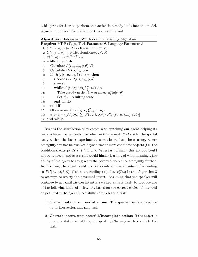
a blueprint for how to perform this action is already built into the model.
Algorithm 3 describes how simple this is to carry out.
Algorithm 3 Interactive Word-Meaning Learning Algorithm
Require: MDP (T, ψ), Task Parameter θ, Language Parameter φ1: Q∗,σ(s, a; θ)← PolicyIteration(θ, T σ, ψ)2: Q∗,ρ(s, a; θ)← PolicyIteration(θ, T ρ, ψ)3: π∗θ(s, a)← eαQ
∗(s,a;θ)/Z4: while 〈s, am〉 do5: Calculate P (i|s, am, φ, θ) ∀i6: Calculate H(I|s, am, φ, θ)7: if H(I|st, am, φ, θ) > τH then8: Choose i ∼ P (i|s, am, φ, θ)9: s′ ← st
10: while s′ 6= argmaxs Vρ∗i
(s′) do
11: Take greedy action a = argmaxa π∗i (a|s′; θ)
12: Set s′ ← resulting state13: end while14: end if15: Observe reaction sτ , aτTτ=0 or am′
16: φ← φ+ ηφ∇φ log[∑
i P (am|i, φ, θ) · P (i|sτ , aτTτ=0, φ, θ)]
17: end while
Besides the satisfaction that comes with watching our agent helping its
tutor achieve his/her goals, how else can this be useful? Consider the special
case, within the basic experimental scenario we have been using, where
ambiguity can not be resolved beyond two or more candidate objects (i.e. the
conditional entropy H(I|·) ≥ 1 bit). Whereas normally this entropy could
not be reduced, and as a result would hinder learning of word meanings, the
ability of the agent to act gives it the potential to reduce ambiguity further.
In this case, the agent could first randomly choose an intent i′ according
to P (I|Am, S, θ, φ), then act according to policy πρ∗i′ (s; θ) and Algorithm 3
to attempt to satisfy the presumed intent. Assuming that the speaker will
continue to act until his/her intent is satisfied, s/he is likely to produce one
of the following kinds of behaviors, based on the correct choice of intended
object, and if the agent successfully completes the task:
1. Correct intent, successful action: The speaker needs to produce
no further action and may rest.
2. Correct intent, unsuccessful/incomplete action: If the object is
now in a state reachable by the speaker, s/he may act to complete the
task.
68
3. Incorrect intent: The speaker must verbally restate his/her request
for the object, as it is still unreachable.
By acting upon the system to move it from s into some new state sx,
and observing the behavior the speaker reacts with ax (which might also be
a state-action sequence), the listener has additional information to use in
calculating the gradient. The information gain, or reduction in entropy fol-
lowing observation of the tutor’s reaction sx, ax to the attempted completion
of goal i, is given by:
IG(I; i = H(I)−H(I |i))
= H(pi, 1− pi), (3.40)
where pi = P (i|am, s, θ, φ). It is straightforward to show that the informa-
tion gain is maximized by selecting the maximum value for the posterior of
i [120]. In the best-case scenario (outcomes 1 or 2 above), entropy can be
eliminated almost entirely. In the worst-case scenario, with n completely
ambiguous intents, the entropy may only be reduced by log2(n+ 1/n) bits.
3.4.4 Discussion
In this section we have presented a so-called “triadic” model for pragmatic
word learning. This model is in effect a unification of many of the principles
and techniques of our initial “basic” and “extended” pragmatic models. As
in the basic model, the inference of linguistic intent is driven by a mirrored
reasoning about the ability of a particular word to affect the desired mental
state (interpretation) in the listener. And as in the extended model, our
agent understands that there is some physical task to which the intended
referent is connected. We consider these two kinds of behaviors — physical
and communicative — as two possible means to the same end. However, in
the case of communicative action, the speaker sees the listener as a potential
path to its goal, and s/he must balance the utility of requesting the user’s
help against his/her own physical ability to achieve the goal.
It is this same reasoning that the listener must use inversely, in order to
recognize the intent underlying an action. As with the extended scenario,
our agent acquires knowledge about the physical task embedded in the in-
teraction, encoded in θ, and uses this to generate representations of utility,
Qσ∗i (s, a; θ) and V σ∗i (s; θ), which could then be used to infer a word’s intent
69
from the speaker’s complementary goal-directed actions. A new line of rea-
soning emerges if our agent also generates these functions in terms of its own
action potential, Qρ∗i (s, a; θ) and V ρ∗i (s; θ). Words as goal-directed actions
are most attractive for a speaker when the value function for the listener,
V ρ∗i (s; θ), is much greater than his/her own, V σ∗
i (s; θ). Therefore, given only
the fact that the speaker chose to communicate anything, the listener may
be able to limit the likely referent to these kinds of intents, without any
need for observing some physical action. This kind of reasoning is based
upon our agent’s understanding of its own embodiment, which influences
the specific potential that it holds to the speaker, and the way in which the
meanings of words are learned. It is this same embodiment that we use to
allow our agent to actively drive its own word learning. This aspect of our
model, while explored in only a very narrow scope, is one that we consider
to hold some of the greatest potential for the future.
70
CHAPTER 4
GROUNDING LANGUAGE IN PERCEPTUAL
REPRESENTATIONS
In the previous chapter, we detailed the model structure and set of learning
algorithms used in creating our “pragmatic engine” for autonomous learn-
ing of word meanings. While the components of the model are rooted in
real-world interactions between embodied agents, the focus has been almost
entirely on cognitive processes operating on internal, symbolic representa-
tions. However, a core premise of this work has been that these symbols
ultimately be grounded in the agent’s representations of perception and ac-
tion, which are themselves connected to the embodiment of the agent, in
our case a humanoid robot.
One of the fundamental challenges of implementing our methods in a real-
world learning environment is the bridging of the noisy, continuous world
of sensory experience with the internal, symbolic world of conceptual rep-
resentations. How does the robot know that a particular word has been
said, or a particular action has been taken? How does the robot even know
what that word sounds like, how does it use that knowledge to recognize
the observed speech segment, and how is the knowledge acquired in the first
place? Before our agent can begin to learn the meanings of words, these
questions must first be addressed. Earlier work of ours sought to do this
through the development of a basic modeling framework, which we applied
in a context of first learning basic action-word groundings, and then apply-
ing this grounded linguistic knowledge to bootstrap the learning of more
complex actions and their linguistic descriptions [10].
4.1 Perceptual Simulators
Our approach was inspired by ideas of perceptual simulators and symbols
proposed by Barsalou [121], for which we developed a two-level perceptual-
conceptual model structure. At the top layer linguistic concepts link per-
ceptual symbols, which index the various perceptual categories present in a
given modality. Perceptual simulators are generative models that represent
71
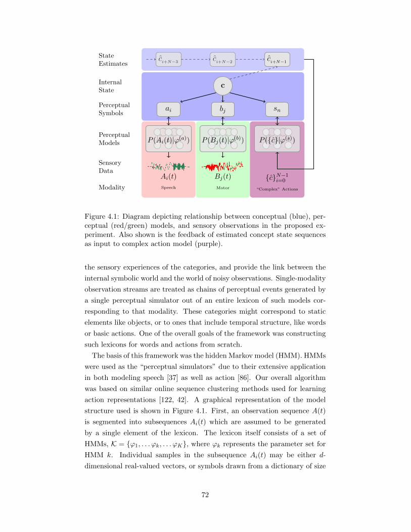
c
ai bj sn
ci+N−3
ci+N−2
ci+N−1
Ai(t) Bj(t) cN−1i=0
Speech Motor “Complex” Actions
PerceptualModels
SensoryData
PerceptualSymbols
InternalState
StateEstimates
Modality
P (Ai(t)|ϕ(a)) P (Bj(t)|ϕ(b)) P (c|ϕ(s))
Figure 4.1: Diagram depicting relationship between conceptual (blue), per-ceptual (red/green) models, and sensory observations in the proposed ex-periment. Also shown is the feedback of estimated concept state sequencesas input to complex action model (purple).
the sensory experiences of the categories, and provide the link between the
internal symbolic world and the world of noisy observations. Single-modality
observation streams are treated as chains of perceptual events generated by
a single perceptual simulator out of an entire lexicon of such models cor-
responding to that modality. These categories might correspond to static
elements like objects, or to ones that include temporal structure, like words
or basic actions. One of the overall goals of the framework was constructing
such lexicons for words and actions from scratch.
The basis of this framework was the hidden Markov model (HMM). HMMs
were used as the “perceptual simulators” due to their extensive application
in both modeling speech [37] as well as action [86]. Our overall algorithm
was based on similar online sequence clustering methods used for learning
action representations [122, 42]. A graphical representation of the model
structure used is shown in Figure 4.1. First, an observation sequence A(t)
is segmented into subsequences Ai(t) which are assumed to be generated
by a single element of the lexicon. The lexicon itself consists of a set of
HMMs, K = ϕ1, . . . ϕk, . . . ϕK, where ϕk represents the parameter set for
HMM k. Individual samples in the subsequence Ai(t) may be either d-
dimensional real-valued vectors, or symbols drawn from a dictionary of size
72
d. Categorizing each Ai(t) received as an element of the lexicon can be done
by the following maximization:
ai = arg maxk∈K
P (Ai(t)|ϕk). (4.1)
The problem for an agent that must learn incrementally from scratch is
that the ϕks are not known in advance, nor is their number. To construct
a lexicon from scratch, we proposed the following basic lexicon learning
algorithm based on a competitive-learning principle. Each time a new Ai(t)
is received, we attempt to classify it as generated by an existing model
ϕk. If the winning model is judged to be a good enough fit, its parameters
are adjusted to fit the new data, while all other models remain the same.
If no model is judged to be a satisfactory fit, a new one is created, and
its parameters are initialized using the sequence as its training data (cf.
equation 2.2). While the expectation-maximization technique [76] is better
suited to the initialization task, we use stochastic gradient techniques [82]
for incremental updates.
One significant issue is determining the methods for judging how well a
model fits the data, also known as the problem of novelty detection. For
our application, we use a novelty detection heuristic similar to one used in
[123]. During the classification step, we calculate both the log-likelihood
Lk = log [P (Ai(t)|ϕk)] and a length-normalized version of the log-likelihood
L. Then a mapping Λk = F(Lk, ϕk) is applied, the purpose of which is to
account for the possible variations in goodness-of-fit that a given perceptual
category can achieve. This mapping is given by
F(Lk, ϕk) =
Lk∫−∞
N (x, µ(ϕk), σ2(ϕk))dx, (4.2)
where the parameters of the Gaussian PDF N (x, µ, σ2) are estimated for
each k from past values of Lk. A threshold τ0 is applied to this mapping
to decide whether the best fitting model is a good enough fit. This entire
procedure is more formally outlined in Algorithm 4.
4.2 Learning of Speech and Action Representations
The lexicon learner is a critical component to the successful implementation
and usage of our pragmatic word leaning model in a real-world human-
robot interaction scenario. In this section, we demonstrate the basis of its
73
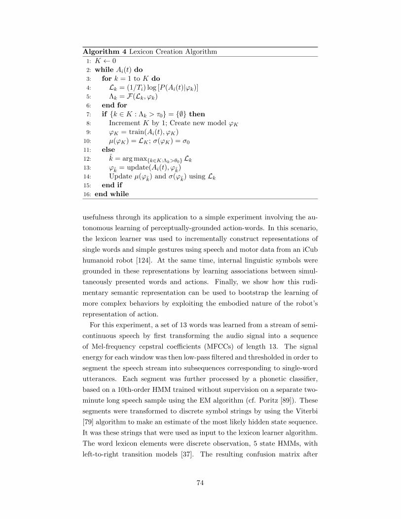
Algorithm 4 Lexicon Creation Algorithm
1: K ← 02: while Ai(t) do3: for k = 1 to K do4: Lk = (1/Ti) log [P (Ai(t)|ϕk)]5: Λk = F(Lk, ϕk)6: end for7: if k ∈ K : Λk > τ0 = ∅ then8: Increment K by 1; Create new model ϕK9: ϕK = train(Ai(t), ϕK)
10: µ(ϕK) = LK ; σ(ϕK) = σ0
11: else12: k = arg maxk∈K:Λk>θ0 Lk13: ϕk = update(Ai(t), ϕk)14: Update µ(ϕk) and σ(ϕk) using Lk15: end if16: end while
usefulness through its application to a simple experiment involving the au-
tonomous learning of perceptually-grounded action-words. In this scenario,
the lexicon learner was used to incrementally construct representations of
single words and simple gestures using speech and motor data from an iCub
humanoid robot [124]. At the same time, internal linguistic symbols were
grounded in these representations by learning associations between simul-
taneously presented words and actions. Finally, we show how this rudi-
mentary semantic representation can be used to bootstrap the learning of
more complex behaviors by exploiting the embodied nature of the robot’s
representation of action.
For this experiment, a set of 13 words was learned from a stream of semi-
continuous speech by first transforming the audio signal into a sequence
of Mel-frequency cepstral coefficients (MFCCs) of length 13. The signal
energy for each window was then low-pass filtered and thresholded in order to
segment the speech stream into subsequences corresponding to single-word
utterances. Each segment was further processed by a phonetic classifier,
based on a 10th-order HMM trained without supervision on a separate two-
minute long speech sample using the EM algorithm (cf. Poritz [89]). These
segments were transformed to discrete symbol strings by using the Viterbi
[79] algorithm to make an estimate of the most likely hidden state sequence.
It was these strings that were used as input to the lexicon learner algorithm.
The word lexicon elements were discrete observation, 5 state HMMs, with
left-to-right transition models [37]. The resulting confusion matrix after
74
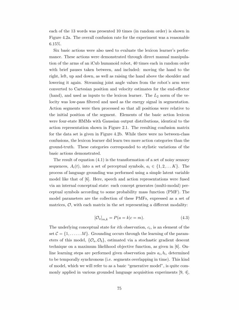
each of the 13 words was presented 10 times (in random order) is shown in
Figure 4.2a. The overall confusion rate for the experiment was a reasonable
6.15%.
Six basic actions were also used to evaluate the lexicon learner’s perfor-
mance. These actions were demonstrated through direct manual manipula-
tion of the arms of an iCub humanoid robot, 40 times each in random order
with brief pauses taken between, and included: moving the hand to the
right, left, up and down, as well as raising the hand above the shoulder and
lowering it again. Streaming joint angle values from the robot’s arm were
converted to Cartesian position and velocity estimates for the end-effector
(hand), and used as inputs to the lexicon learner. The L2 norm of the ve-
locity was low-pass filtered and used as the energy signal in segmentation.
Action segments were then processed so that all positions were relative to
the initial position of the segment. Elements of the basic action lexicon
were four-state HMMs with Gaussian output distributions, identical to the
action representation shown in Figure 2.1. The resulting confusion matrix
for the data set is given in Figure 4.2b. While there were no between-class
confusions, the lexicon learner did learn two more action categories than the
ground-truth. These categories corresponded to stylistic variations of the
basic actions demonstrated.
The result of equation (4.1) is the transformation of a set of noisy sensory
sequences, Ai(t), into a set of perceptual symbols, ai ∈ 1, 2, . . .K. The
process of language grounding was performed using a simple latent variable
model like that of [6]. Here, speech and action representations were fused
via an internal conceptual state: each concept generates (multi-modal) per-
ceptual symbols according to some probability mass function (PMF). The
model parameters are the collection of these PMFs, expressed as a set of
matrices, O, with each matrix in the set representing a different modality:
[Oa]m,k = P (a = k|c = m). (4.3)
The underlying conceptual state for ith observation, ci, is an element of the
set C = 1, . . . . . .M. Grounding occurs through the learning of the param-
eters of this model, Oa,Ob, estimated via a stochastic gradient descent
technique on a maximum likelihood objective function, as given in [6]. On-
line learning steps are performed given observation pairs ai, bi, determined
to be temporally synchronous (i.e. segments overlapping in time). This kind
of model, which we will refer to as a basic “generative model”, is quite com-
monly applied in various grounded language acquisition experiments [9, 4],
75
# of Classifications as Lexical Element
Confusion Matrix for Word Lexicon
Sp
oke
n W
ord
1 2 3 4 5 6 7 8 9 10 11 12 13
"left"
"right"
"raise"
"lower"
"up"
"down"
"chop"
"shake"
"brush"
"greet"
"sweep"
"hand"
"wave"
0 1 2 3 4 5 6 7 8 9 10
(a) Word confusion matrix.
# of Classifications as Lexical Element
Confusion Matrix for Action Lexicon
De
mo
nstr
ate
d A
ctio
n N
am
e
1 2 3 4 5 6 7 8
left
right
raise
lower
up
down
0 5 10 15 20 25 30 35 40
(b) Action confusion matrix.
Figure 4.2: Confusion matrices for word and action lexicon learning tasks.Ordinate labels are given only denote the “ground-truth” action/word cat-egories intended by the tutor, and were not provided to the robot duringtraining.
76
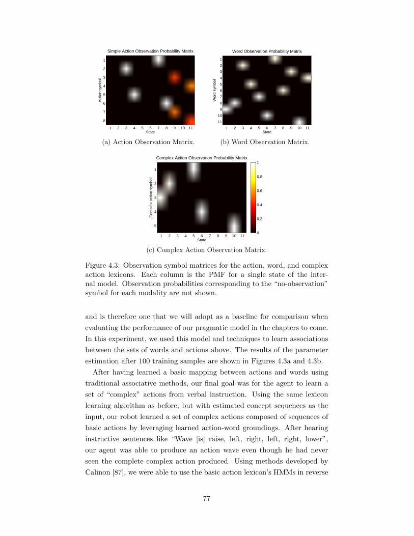
State
Act
ion
sym
bol
Simple Action Observation Probability Matrix
1 2 3 4 5 6 7 8 9 10 11
1
2
3
4
5
6
7
8
(a) Action Observation Matrix.
State
Wor
d sy
mbo
l
Word Observation Probability Matrix
1 2 3 4 5 6 7 8 9 10 11
1
2
3
4
5
6
7
8
9
10
11
(b) Word Observation Matrix.
State
Com
plex
act
ion
sym
bol
Complex Action Observation Probability Matrix
1 2 3 4 5 6 7 8 9 10 11
1
2
3
4
5
0
0.2
0.4
0.6
0.8
1
(c) Complex Action Observation Matrix.
Figure 4.3: Observation symbol matrices for the action, word, and complexaction lexicons. Each column is the PMF for a single state of the inter-nal model. Observation probabilities corresponding to the “no-observation”symbol for each modality are not shown.
and is therefore one that we will adopt as a baseline for comparison when
evaluating the performance of our pragmatic model in the chapters to come.
In this experiment, we used this model and techniques to learn associations
between the sets of words and actions above. The results of the parameter
estimation after 100 training samples are shown in Figures 4.3a and 4.3b.
After having learned a basic mapping between actions and words using
traditional associative methods, our final goal was for the agent to learn a
set of “complex” actions from verbal instruction. Using the same lexicon
learning algorithm as before, but with estimated concept sequences as the
input, our robot learned a set of complex actions composed of sequences of
basic actions by leveraging learned action-word groundings. After hearing
instructive sentences like “Wave [is] raise, left, right, left, right, lower”,
our agent was able to produce an action wave even though he had never
seen the complete complex action produced. Using methods developed by
Calinon [87], we were able to use the basic action lexicon’s HMMs in reverse
77

−0.2
0
0.20.3
0.4
0
0.2
0.4
x (m)
Human Demonstration
y (m)
z (
m)
(a) Human generated wave.
−0.2
0
0.20.3
0.4
0
0.2
0.4
x (m)
Robot Demonstration
y (m)
z (
m)
(b) Robot generated wave.
Figure 4.4: Comparison of human demonstration and robot reproduction ofthe complex action labeled “wave”, represented as hand trajectory expressedin Cartesian coordinates.
to generate example sequences. This same generative ability was used for
the complex action to chain together sequences of basic actions to produce
the previously unseen composite action “wave”. A comparison between an
example produced by the human tutor and one constructed by the robot is
shown in Figure 4.4.
The fundamental purpose of this small experiment was twofold. The
first goal was simply to confirm that the algorithm could be practically
implemented and perform its intended function — the autonomous learning
of basic perceptual representations from noisy sensorimotor experience. Its
second purpose was to provide a more concrete demonstration of how the
model can be practically applied to speech and motor function. This will be
relevant primarily for speech in application to the pragmatic model. We will
use the same incremental lexicon learning algorithm to build representations
of word symbols (which we denoted as discrete speech actions am in the
pragmatic model), from segmented streams of speech.
These techniques will, however, be less applicable to creating representa-
tions of action. The primary reason for this is the goal-based representation
of action in our pragmatic model. We will see in the coming chapter that
while this representation is embedded in a relatively low-level perception of
space, and its parameterization θ is learned in an online manner, its connec-
tion to sensory and perceptual data is ultimately fixed. This is due in large
part to the relative lack of computationally tractable methods for solving
the inverse planning or reinforcement learning problems in continuous state
78

and action spaces. However, some recent techniques for learning among a set
of candidate reward functions in continuous spaces, using Gaussian mixture
models [125], hold the possibility for future extension to our model.
79
CHAPTER 5
ROBOT IMPLEMENTATION
In this chapter, we will more concretely detail how the models and algo-
rithms developed in Chapters 3 and 4 are applied to the general set of
human-robot interaction scenarios presented in Chapter 6. After first dis-
cussing the particular embodiment of our agent — the iCub humanoid robot
— we will outline how the various elements of the pragmatic model are im-
plemented. For those parts of the model for which we have made simplifying
assumptions about the structure of perceptual representations, we will detail
the processing capabilities that support their function.
5.1 The iCub Humanoid Robot
In our real-world implementations, we will be using the iCub as our embod-
ied platform [124]. The iCub is a humanoid robot with the capability to move
its head, neck, torso, arms, legs, and hands through 53 motors, 18 of which
are in the hands alone. In addition to standard position/velocity control,
strain gauges in the hips and shoulders allow for force/torque/impedance
control. Beyond its proprioceptive capabilities, the iCub is also outfitted
with two color cameras that can stream 640 × 480 images at a rate of 30
frames per second. Two microphones are embedded in a head casing fea-
turing artificial asymmetrical pinnae, allowing for better sound localization.
Interfacing with the robot is facilitated by the YARP middleware package
[126]. Owing to its open-source philosophy, both of these packages have
come to see widespread use as standard hardware/software platforms for
cognitive robotics research. As a result, there exists a large number of im-
plementations of common algorithms shared among the community, many
of which we use in support of this proposed work (e.g. Cartesian and gaze
controllers [127, 128]). Because of its extensive sensorimotor periphery and
a software system that supports efficient real-time communication with the
robot, the iCub is well suited for our proposed application.
80
5.2 Application of the Pragmatic Model
In the discussion of the pragmatic engine, the elements of the model shown
in Figure 3.2 were treated in largely abstract terms, with only a general
description of their relationship to the human-robot interaction scenario.
These elements were the states of the environment, intentional states, and
physical and linguistic (words) actions. Also included were a number of
models and functions that determine the dynamics of the states and ac-
tions, such as the state-action transition model, the task and word meaning
parameters, and the mapping from states to features. In this section, we
detail more clearly how these are all defined and implemented in the human-
robot interaction experiments. This includes the algorithms and procedures
for how they are processed and estimated using the noisy perceptual data
streamed from the robot.
5.2.1 Physical Elements
World State
Chapter 3 defined the world or environment state S as the Cartesian product
of the individual state spaces for the speaker, listener, and all objects: S =
Sσ×Sρ×So1×. . .SoN . For all of the experiments considered in this thesis, an
agent or object’s state will correspond to its spatial location, or the location
of its end-effector in the case of agents. We will further define this location
to refer only to the X and Y positions of the object with respect to the
robot’s root reference frame. This simplification relies on our assumption
that the objects are all situated on a common Z coordinate plane (i.e. the
table). Each possible value for an object’s state corresponds to the location
of that object at a particular (x, y) location. For our implementation, these
locations are spaced evenly in the x and y directions across the workspace,
which we assume to be bounded between (xmin, xmax) and (ymin, ymax).
This forms a Mx×My grid, and results in object state spaces that are each
Mx ·My large.
An object’s state at any given time must be determined from some continuous-
valued location measurement (X(t), Y (t)). One approach might be to simply
find the state corresponding to the grid center location (cx, cy) that is closest
to the measurement. Such winner-take-all state decisions might have nega-
tive effects on the calculation of the empirical observation statistics µE and
πE that are needed for learning of the task parameter in equation (3.28),
81
especially when measurements (X(t), Y (t)) are nearly equally close to many
state centers. A better method might be to smooth these statistical calcu-
lations by calculating a probability mass function (PMF) over the states:
P (St = s(k)|X(t), Y (t)) ∝ P (X(t)|St = s(k))P (Y (t)|St = s(k))
= N (X(t); cxk , σ2x) · N (Y (t); cyk , σ
2y). (5.1)
The specific values chosen for σx and σy will influence the amount of smooth-
ing that occurs across states.
Actions
The actions discussed for our pragmatic model were of two types: physical
and linguistic. The latter types were the set of symbols corresponding to
spoken words, and their representation and perception is covered by the
methods and models described in Chapter 4. For now we focus on physical
actions, which we previously assumed to be the union of the spaces of actions
that an agent could take on individual objects: Aσp = (Ao1⋃. . .AoN ). Note
that these action spaces are dependent on the particular agent, and may
not be the same for each agent. Furthermore, the possible actions for each
object may also not be the same.
For our human-robot interaction experiments, we will consider the set
of physical actions to be some discrete set of possible spatial movements
of the objects. We will use the set of actions corresponding to movements
in the four ordinal directions (up, down, left, right), as well as the case
where there is no (or nearly no) movement. As with the state space above,
observations of actions must be determined on the basis of continuous-valued
perceptual data. In this case, the perceptual data are the discrete-time
difference measurements (X(t), Y (t)), where X(t) = X(t) − X(t − 1). As
before, we would like to calculate a PMF over this set of discrete actions,
rather than trying to produce a single point estimate of the observed action.
Unlike before, however, our action classes are determined by movement in
some particular direction (i.e. downward), not necessarily a particular range
of values for X or Y . Therefore, we first find the normalized movement
vector:
82
D(t) , (X(t), Y (t)),
D(t) =D(t)
‖ D(t) ‖2. (5.2)
Ideally, the probability of D being one of the ordinal movements should be
proportional to how close it is to the unit vector for that movement δa:
P (a|D(t)) ∝ eσd‖D(t)−δa‖22 . (5.3)
However, we must also account for the no-movement case, which cor-
responds to small magnitudes of D. To do this, we heuristically let the
probability of a “no-move” action be proportional to the magnitude of the
original D(t):
P (a0|D(t)) ∝ eσd‖D(t)‖22 . (5.4)
As with the state probabilities, the specific value chosen for the parameter
σd will control the smoothness of the PMF across the actions.
State and Action Dynamics
One of the critical components of our pragmatic engine is the model of state
and action dynamics, or the model of how actions influence the evolution
of the world state from one time step to the next. This “transition” model
is the same one that is central to the Markov decision process (MDP) upon
which much of our framework is based. We define the following notation for
the transition model, T :
[T ]ijk = P (St+1 = k|St = i, At = j), (5.5)
where∑k
Tijk = 1. For the most part, we consider the state and action
models to be factored on the basis of the objects they represent. This
means that actions on a particular object will affect only the state of that
object, and no others, resulting in much simpler computation for calculations
involving T . Relaxing this assumption would surely be beneficial to the
83
model’s ability to represent complex physical interactions, but it would also
cause a significant increase in computational complexity.
Recalling the grid-based state space for individual objects, and our rep-
resentation of actions as single movements along this grid, we describe the
following implementation for the state-action transition model. Let s(k) be
the currently occupied state for an object, and let s(l) be the state directly
above it in the grid. We then define:
P (St+1 = s|St = s(k), At = aup) =
ζ if s = s(l)
ζ/8 if s 6= s(l), d(s, s(l)) ≤√
2, (5.6)
where d(s, s′) is the Euclidean distance in grid units between state s and
s′. This means that there is some probability that a move along the grid
will result in reaching the “ideal” location, plus all adjoining locations on
the grid. The formulation in equation (5.6) is the same for moves in all four
directions, as well as the “no move” case. A typical value used for the ζ
above in our implementations is 0.9.
There are also situations in many of our human-robot interaction experi-
ments where an object may not be moved freely in some direction, for reasons
such as the presence of a physical barrier or other constraints on its motion.
In these cases, transition probabilities into states corresponding to locations
of obstructions are set to 0, and the values of the PMF are re-normalized. If
the object is in a location where an agent is unable to reach it or otherwise
act upon it, transition probabilities are set to 1 for self-transitions, and 0
for all else, for each action.
5.2.2 Intentional and Belief Elements
In our framework, we have used the word “intent” to refer to the goal an
agent is trying to reach through its behavior, a concept which is embedded
in the MDP and its formulation of the reward function. However, we have
noted that one of the core premises of this thesis is that even though reward
functions may span the entire state space (or even more complex spaces),
the number of actual potential rewards we search over is far smaller. The
interactions which we target are structured in a way that rewards can be
generated from more compact sets of parameters and variables, which have
complex connections to linguistic representations. In order to greatly sim-
plify the problem of learning these connections between words and intents,
84
we have assumed a particular structure for the interaction format, its gen-
eral task, and the variable aspects of the intent. Under this assumption,
intent states are the possible objects for which some general task is being
performed. This was captured in our formulation for the reward function
given in equation (3.19):
Ri(s; θ) = θTψ(gi(s)). (5.7)
Intents
The space of possible values for the intentional state are the indices of possi-
ble objects upon which the desired task is to be performed: I ∈ 1, 2, . . . N.The set of potential intended objects does not necessarily have to be equal
to the set of all objects present in the current environment, but we do as-
sume it to be a subset of this larger set for our implementation. All of
the objects have some corresponding spatially defined state, as detailed in
equation (5.1). An object is perceived visually, requiring our robot to be
capable of segmenting the objects within an image and estimating their lo-
cation through some means (e.g. stereopsis). We will detail the processing
system for performing these functions in Section 5.3.
One of the key functions of the intentional state is to serve as an argument
of the reward generating function above. Specifically, we have defined a
function gi(s) that effectively selects the subset of the complete state space
over all objects that are specific to a particular intended object: gi : S → Si.In some of our experiments, Si may be strictly equal to the individual state
space for the object, Soi. For others, it may also include the states of
other “auxiliary” objects that are important to the overall task, but are not
part of the set of possible intents. The same is also true for the function
hi : A → Ai, which performs the same kind of selection over the space of
actions.
State Features and Task Parameters
Our interaction formats also include an invariant, “task” component, which
is the goal to be satisfied for an intended object, regardless of the specific
object that has been selected. After an intent-specific reduced state space
Si has been selected, the function ψ(s) extracts the value of the “features”
for each state: ψ : S → Rf . The values of the task parameter vector
85
θ ∈ Rf are the weights applied to each feature before summing to find the
reward value at that state. For some scenarios, we use a straightforward
implementation of the feature function, where f = |S|, and ψ(s) = 1 only
for the s-th feature, and 0 for all else. In this case, the task parameter
becomes effectively a standard vector for the reward values at each state.
In other cases, specifically those for which the task involves both an in-
tentional and auxiliary object, we use a more complex feature space. This
includes the above features for each of the intended and auxiliary objects,
as well as features that are functions of both objects. These might be fea-
tures such as the distance between the objects, or their relative positions.
In either of these cases, we will see that the unsupervised inverse reinforce-
ment learning (IRL) technique will learn what features in this more complex
representation are relevant to the observed task.
5.3 Visual Processing
Proper perception of many of the elements of this model rely on complex ca-
pabilities for the processing of visual information. These include the ability
to not only segment and track multiple objects within a stream of images,
but also the ability to determine its spatial location and movements. There
are also other kinds of social information useful to our experiments, such
as gaze, that must be determined through visual processing. Many of these
processing capabilities are built upon one another (as depicted in Figure
5.1), and therefore require computationally efficient algorithms in order to
be capable of real-time processing for successful interaction. In this section,
we discuss the techniques we use for the object segmentation, tracking, and
localization problems, as well as our method for generating joint attentional
saliency information from gaze features based on an artificial neural network.
5.3.1 Object Segmentation and Tracking
In order to vastly simplify the complexity of the object segmentation and
tracking task, we first make a handful of assumptions based on our training
scenarios:
1. The interaction environment consists of a largely white background
and workspace (table), on which the objects are placed.
2. The objects are generally colorful in nature, in order to ease the prob-
lem of separating foreground pixels from the background.
86
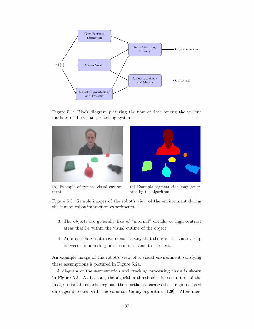
M(t) Stereo Vision
Gaze Feature/Extraction
Object Segmentation/and Tracking
Joint Attention/Saliency
Object Location/and Motion
Object saliencies
Object x,x
Figure 5.1: Block diagram picturing the flow of data among the variousmodules of the visual processing system.
(a) Example of typical visual environ-ment.
(b) Example segmentation map gener-ated by the algorithm.
Figure 5.2: Sample images of the robot’s view of the environment duringthe human-robot interaction experiments.
3. The objects are generally free of “internal” details, or high-contrast
areas that lie within the visual outline of the object.
4. An object does not move in such a way that there is little/no overlap
between its bounding box from one frame to the next.
An example image of the robot’s view of a visual environment satisfying
these assumptions is pictured in Figure 5.2a.
A diagram of the segmentation and tracking processing chain is shown
in Figure 5.3. At its core, the algorithm thresholds the saturation of the
image to isolate colorful regions, then further separates these regions based
on edges detected with the common Canny algorithm [129]. After mor-
87
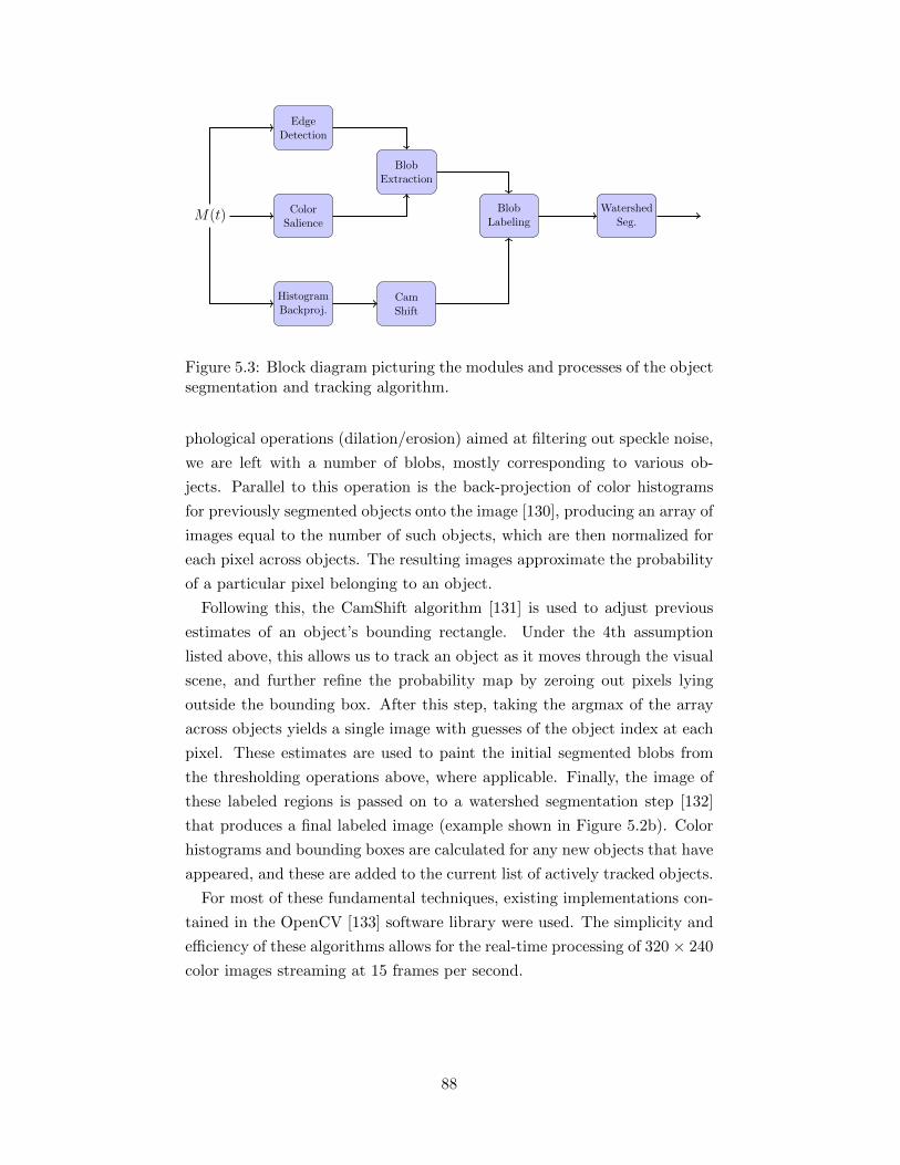
M(t) ColorSalience
EdgeDetection
HistogramBackproj.
BlobExtraction
CamShift
BlobLabeling
WatershedSeg.
Figure 5.3: Block diagram picturing the modules and processes of the objectsegmentation and tracking algorithm.
phological operations (dilation/erosion) aimed at filtering out speckle noise,
we are left with a number of blobs, mostly corresponding to various ob-
jects. Parallel to this operation is the back-projection of color histograms
for previously segmented objects onto the image [130], producing an array of
images equal to the number of such objects, which are then normalized for
each pixel across objects. The resulting images approximate the probability
of a particular pixel belonging to an object.
Following this, the CamShift algorithm [131] is used to adjust previous
estimates of an object’s bounding rectangle. Under the 4th assumption
listed above, this allows us to track an object as it moves through the visual
scene, and further refine the probability map by zeroing out pixels lying
outside the bounding box. After this step, taking the argmax of the array
across objects yields a single image with guesses of the object index at each
pixel. These estimates are used to paint the initial segmented blobs from
the thresholding operations above, where applicable. Finally, the image of
these labeled regions is passed on to a watershed segmentation step [132]
that produces a final labeled image (example shown in Figure 5.2b). Color
histograms and bounding boxes are calculated for any new objects that have
appeared, and these are added to the current list of actively tracked objects.
For most of these fundamental techniques, existing implementations con-
tained in the OpenCV [133] software library were used. The simplicity and
efficiency of these algorithms allows for the real-time processing of 320 × 240
color images streaming at 15 frames per second.
88
5.3.2 Estimation of Location and Motion
Given a consistent labeling of segmented objects from image to image, it is
now possible for us to reliably keep track of an object’s spatial location and
movement over the course of the interaction. To do this, we make use of
the iCub’s binocular vision capabilities, and the OpenCV implementation
of the Semi-Global Block Matching (SGBM) algorithm to compute a dense
disparity/depth map for the visual environment [134]. This depth map
can be transformed through the iCub’s forward kinematics to produce a
Cartesian XYZ for each pixel relative to the root reference frame of the
robot [135].
Combined with the segmentation map, a list of 3-D spatial locations for
pixels corresponding to each object can be generated. But in order to do
this, there are a number of questions and challenges to be addressed. The
first is picking a method for producing a single point estimate for an object’s
position from the point cloud of single-pixel estimates. The most intuitive
method might be to simply calculate the mean or median value of the list
of points, or some other method for approximating the geometric center of
the point cloud.
The second major challenge is producing a location estimate that is reli-
able, given the potentially significant noise and inaccuracy in the single-point
measurements of the cloud. While calculating a statistic such as mean or
median can handle some amount of uncertainty, they generally require both
the points and their noise to be normally distributed around the object cen-
ter, which is the case much of the time. But often times, situations in which
the object is occluded, is moving, or has a lack of defining visual features,
will result in 3-D point estimates that contain significant clusters at other
spatial locations, in addition to a number of other outliers. This can produce
location estimates that vary significantly from frame-to-frame as an object
moves or comes close to other objects.
To mitigate this problem, we return to some of the same simplifying as-
sumptions we used in the development of our segmentation and tracking
algorithm, specifically those dealing with the location of our objects on a
table, and their expected movement from frame to frame. But this time
we consider their spatial, rather than spectral, implications. Since we as-
sume to know the presence of objects on a flat table, we are able to discard
points for the objects that are estimated to be below the general plane of
the table (Z < −0.3). Next, we assume that the movement of the object
in space will not be greater than roughly 3 m/s in any direction. For our
89
robotic implementation, images are streamed from the cameras at 15 frames
per second, which means we do not expect the object’s position to differ by
more than 0.2 m from one frame to the next. Therefore, we reject as outliers
any estimated points for an object whose Euclidean distance to the previous
estimated location of the object is greater than 0.2 m. After this rejection
step, we simply estimate the new spatial location of the object using the
mean or median of the point cloud as before.
5.3.3 Gaze Estimation and Joint Attention
Another supporting skill that is critical to a real-world robotic implemen-
tation is that of joint attention. The joint attentional faculty allows agents
to socially construct shared attentional frames, which is the entirety of ob-
jects or events that the interacting agents commonly know to be possible
targets of attentional focus within the scenario. This faculty includes both
the ability to recognize another’s attentional focus, and the complementary
ability to use one’s own attentional focus to direct the attention of another
[136, 74]. As we have discussed in previous chapters, recognizing possible
attentional states of a speaker is often a key piece of information in narrow-
ing the range of possibilities for his/her referential intent. We therefore seek
to implement some small processing mechanism for using joint attentional
cues to serve as a “social spotlight” in service of the word-learning problem
[4]. The goal of this capability is only for the purpose of partially reducing
the ambiguity of the speaker’s intent in the initial tests of our pragmatic
model — where no other information about intent is available — and is not
used to reduce it completely.
The active and passive aspects of joint attention — the ability to direct
another’s attention and the ability to follow this direction, respectively —
are two sides of the same coin. Recognition of another’s attentional focus is
in large part the recognition of their directive action. Humans are able to
direct attention both through linguistic behaviors (e.g. “Look at the ball!”)
as well as non-linguistic behaviors (e.g. pointing). The latter category of
behaviors is perhaps the most important for the pre-/early-linguistic children
that are our focus. Primary among these is use of gaze-direction for direction
and inference of attentional focus.
Determining the object or event of focus from gaze requires an agent first
to visually estimate the head and eye pose of the other agent, and then
map this gaze-direction onto some area of the environment. This map can
be constructed on the basis of predetermined geometric knowledge, or it
90
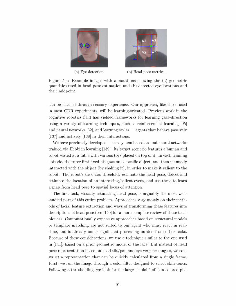
(a) Eye detection. (b) Head pose metrics.
Figure 5.4: Example images with annotations showing the (a) geometricquantities used in head pose estimation and (b) detected eye locations andtheir midpoint.
can be learned through sensory experience. Our approach, like those used
in most CDR experiments, will be learning-oriented. Previous work in the
cognitive robotics field has yielded frameworks for learning gaze-direction
using a variety of learning techniques, such as reinforcement learning [95]
and neural networks [32], and learning styles — agents that behave passively
[137] and actively [138] in their interactions.
We have previously developed such a system based around neural networks
trained via Hebbian learning [139]. Its target scenario features a human and
robot seated at a table with various toys placed on top of it. In each training
episode, the tutor first fixed his gaze on a specific object, and then manually
interacted with the object (by shaking it), in order to make it salient to the
robot. The robot’s task was threefold: estimate the head pose, detect and
estimate the location of an interesting/salient event, and use these to learn
a map from head pose to spatial locus of attention.
The first task, visually estimating head pose, is arguably the most well-
studied part of this entire problem. Approaches vary mostly on their meth-
ods of facial feature extraction and ways of transforming these features into
descriptions of head pose (see [140] for a more complete review of these tech-
niques). Computationally expensive approaches based on structural models
or template matching are not suited to our agent who must react in real-
time, and is already under significant processing burden from other tasks.
Because of these considerations, we use a technique similar to the one used
in [141], based on a prior geometric model of the face. But instead of head
pose representation based on head tilt/pan and eye vergence angles, we con-
struct a representation that can be quickly calculated from a single frame.
First, we run the image through a color filter designed to select skin tones.
Following a thresholding, we look for the largest “blob” of skin-colored pix-
91
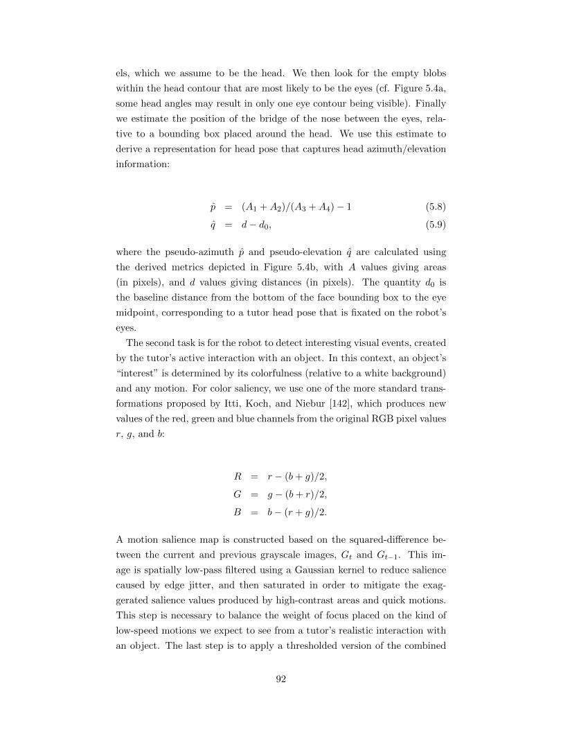
els, which we assume to be the head. We then look for the empty blobs
within the head contour that are most likely to be the eyes (cf. Figure 5.4a,
some head angles may result in only one eye contour being visible). Finally
we estimate the position of the bridge of the nose between the eyes, rela-
tive to a bounding box placed around the head. We use this estimate to
derive a representation for head pose that captures head azimuth/elevation
information:
p = (A1 +A2)/(A3 +A4)− 1 (5.8)
q = d− d0, (5.9)
where the pseudo-azimuth p and pseudo-elevation q are calculated using
the derived metrics depicted in Figure 5.4b, with A values giving areas
(in pixels), and d values giving distances (in pixels). The quantity d0 is
the baseline distance from the bottom of the face bounding box to the eye
midpoint, corresponding to a tutor head pose that is fixated on the robot’s
eyes.
The second task is for the robot to detect interesting visual events, created
by the tutor’s active interaction with an object. In this context, an object’s
“interest” is determined by its colorfulness (relative to a white background)
and any motion. For color saliency, we use one of the more standard trans-
formations proposed by Itti, Koch, and Niebur [142], which produces new
values of the red, green and blue channels from the original RGB pixel values
r, g, and b:
R = r − (b+ g)/2,
G = g − (b+ r)/2,
B = b− (r + g)/2.
A motion salience map is constructed based on the squared-difference be-
tween the current and previous grayscale images, Gt and Gt−1. This im-
age is spatially low-pass filtered using a Gaussian kernel to reduce salience
caused by edge jitter, and then saturated in order to mitigate the exag-
gerated salience values produced by high-contrast areas and quick motions.
This step is necessary to balance the weight of focus placed on the kind of
low-speed motions we expect to see from a tutor’s realistic interaction with
an object. The last step is to apply a thresholded version of the combined
92
color salience map T (Ct) as a mask to the post-processed motion salience
image Ht and run it through a leaky integrator to get the final combined
salience map St:
St = T (Ct) · [Ht + (1− α)St−1] , (5.10)
where α is the leakage constant, which has values on the order of 1× 10⁻³
for our experiments. This leaky integration selects for objects exhibiting
sustained activity by building up salience values for moving objects over
time. When a point or “blob” of points exceeds a set salience threshold τ ,
its (x, y) location (or the location of the blob’s centroid) is paired with the
current estimate of the head pose (p, q) and used as a training sample for
the map.
The map itself is called upon in two different situations. The first is the
training situation described above, where both input and output values for
the map are provided. The second is the prediction situation, where the
agent only has access to a head pose (p0, q0), and must use the map to
estimate the location the tutor is attending to. For our application, we
would like these situations to be in free variation within a larger online
learning scenario. To do this, we need a model and a learning rule capable
of incremental updating and on-the-fly prediction. Specifically, we use an
artificial neural network composed of an input, output, hidden input, and
hidden output layers. The hidden layers are connected by a set of weights
wij , with i indexing the outer hidden neurons, and j indexing the inner.
Activations of the inner and outer hidden layers are generated by the input
and output neurons using radial basis functions (RBFs). These RBFs are
normalized Gaussian functions centers ci and cj , and widths Σi and Σj . Even
with their relatively simple structure, RBFNNs are capable of approximating
any arbitrary mapping, such as our target mapping, (p, q)→ (x, y).
We assign the centers cj and ci for hidden inner and outer neurons so that
they are evenly distributed across the input and output spaces. Internal
weights wij are updated each time a training sample is received using a
generalized Hebbian learning-like rule [143], with learning rate η and leakage
coefficient ε (a typical heuristic used to mitigate the effect of outliers):
w(t+1)ij = εw
(t)ij + η(Fij(p, q, xt, yt)− Fi(xt, yt)W T
j F (xt, yt)). (5.11)
The term Fij(p, q, xt, yt) above is the complete activation of each neuron at
time t, which can be factored into the inner and outer hidden layer activa-
93
tions Fj(p, q, t)Fi(xt, yt). As stated, the individual F s are calculated from
Gaussian RBFs — for example, Fi(xt, yt) is given by N (x, y; ci; Σi), where
ci = [cxi , cyi ] and Σi is diagonal. It is worth noting that only one hidden
layer is theoretically needed to learn our arbitrary mapping. Because early
sampling of input and output spaces is quite sparse, however, the smoothing
of activations on both input and output aids in generalization, even for low
numbers of training samples.
In non-training episodes, the gaze location (x, y) can be predicted using
the estimated head pose and the current value of the learned weights. To do
this, we first multiply the trained weight matrix W by the inner activation
vector Fj(pt, qt) and re-normalize to generate the predicted outer activation,
which we denote Fi(xt, yt). The following equation shows how to calculate
the predicted output activation x, with a similar result holding for y as well:
x =N∑i=1
ciFi(xt, yt). (5.12)
While exact values for x and y are mathematically pleasing, they may not
be as practically useful for our application, where we would like to estimate
the possible object(s) of attention. One naive approach might be to derive a
distribution over objects based on their distance from (x, y), but calculating
this distance correctly would require further processing to correct for spatial
distortion caused by orthogonal projection. Fortunately, such information
is already built into our network, which learns the shape of this arbitrary
mapping, distortion included. Instead of calculating attention as a specific
point, we reorganize the predicted outer activations Fi(xt, yt) into a grid
based on their corresponding [cxi , cyi ] values. We then up-sample this to our
original full-image resolution and low-pass filter to produce what itself can
be thought of as a saliency map, which we denote with Jt. Using the same
thresholded color salience map as before (cf. equation 5.10) to mask Jt, we
can calculate a salience score for each object blob, consisting of set of pixels
Bk:
zk =∑b∈Bk
Jt(b) · T (Ct(b)). (5.13)
The joint saliency scores for each object zk, can be used to construct a
probability distribution for the attentional state through use of a softmax
or other typical non-linear activation function. Figures 5.5a and 5.5b show
an example calculation of Jt and its application to selecting the object of
maximum attentional salience. This probability distribution can be used
94
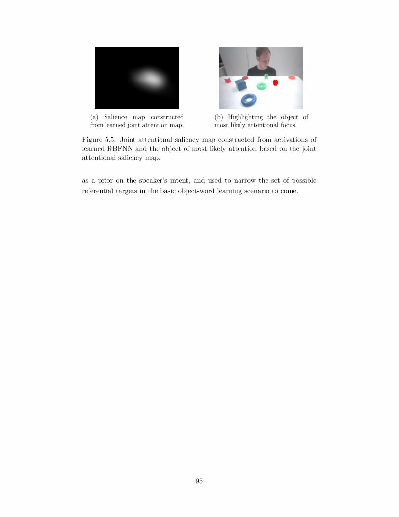
(a) Salience map constructedfrom learned joint attention map.
(b) Highlighting the object ofmost likely attentional focus.
Figure 5.5: Joint attentional saliency map constructed from activations oflearned RBFNN and the object of most likely attention based on the jointattentional saliency map.
as a prior on the speaker’s intent, and used to narrow the set of possible
referential targets in the basic object-word learning scenario to come.
95
CHAPTER 6
HUMAN-ROBOT INTERACTION
EXPERIMENTS
In this chapter, we present the results of the application of the models and
methods developed in the previous chapters to a set of human-robot inter-
action experiments. These are based on a select group of experiments —
found in the developmental literature concerning early language acquisition
— that were used as the motivating examples during the development of our
computational framework. While our scenarios are not exact reproductions,
they are intended to evaluate the same kinds of core pragmatic abilities
thought to be used by children to resolve referential ambiguity in these ex-
periments. These include not only the principles of cross-situational learning
and lexical contrast present in current embodied word-learning frameworks,
but also those that are more specific to our model, such as learning from
goal-directed behaviors, or leveraging information about action constraints
and triadic interaction structure.
6.1 Experiment I: Pragmatic Learning of BasicObject-Words
The experiment we perform is of a very simple nature, primarily attempting
to evaluate the fundamental soundness of the learning algorithms derived for
the basic pragmatic model. The goal of our framework in this case is to learn
a set of words and how they are used to refer to various objects in the visual
space (i.e. their meaning). In our experiments, we seek to demonstrate the
ability of our model to learn from observations featuring referential ambigu-
ity through the use of basic statistical processing capabilities and emergent
lexical contrast principles, in line with the results of previous work [4, 53].
Finally, for these initial experiments and those that follow, training data is
presented continuously, requiring the use of real-time perception and online
learning techniques developed in the previous chapters.
96
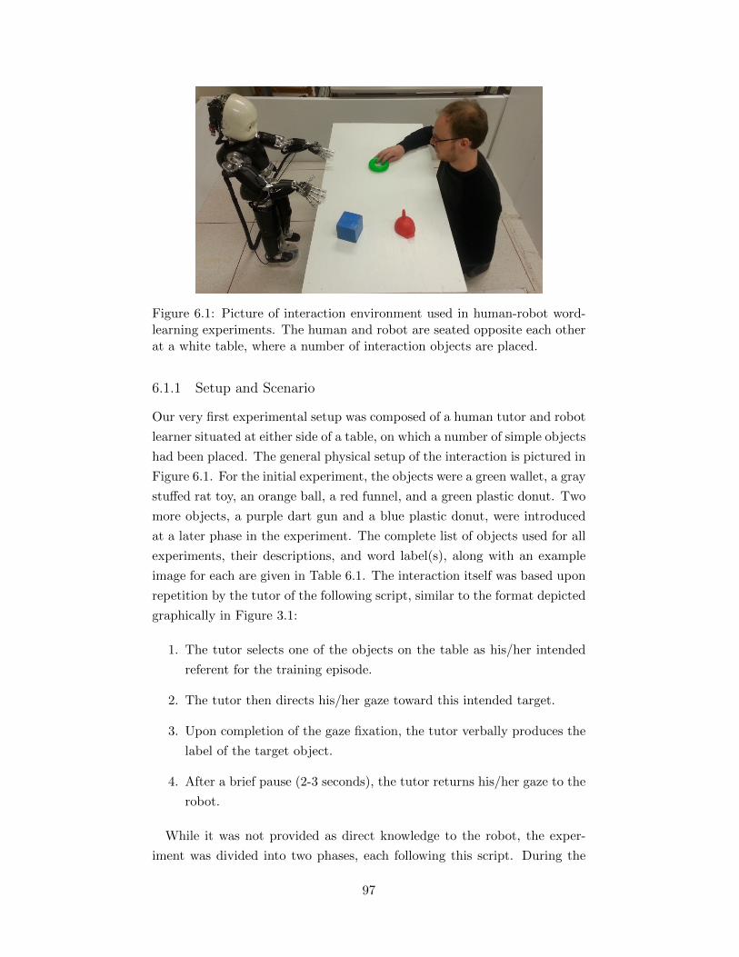
Figure 6.1: Picture of interaction environment used in human-robot word-learning experiments. The human and robot are seated opposite each otherat a white table, where a number of interaction objects are placed.
6.1.1 Setup and Scenario
Our very first experimental setup was composed of a human tutor and robot
learner situated at either side of a table, on which a number of simple objects
had been placed. The general physical setup of the interaction is pictured in
Figure 6.1. For the initial experiment, the objects were a green wallet, a gray
stuffed rat toy, an orange ball, a red funnel, and a green plastic donut. Two
more objects, a purple dart gun and a blue plastic donut, were introduced
at a later phase in the experiment. The complete list of objects used for all
experiments, their descriptions, and word label(s), along with an example
image for each are given in Table 6.1. The interaction itself was based upon
repetition by the tutor of the following script, similar to the format depicted
graphically in Figure 3.1:
1. The tutor selects one of the objects on the table as his/her intended
referent for the training episode.
2. The tutor then directs his/her gaze toward this intended target.
3. Upon completion of the gaze fixation, the tutor verbally produces the
label of the target object.
4. After a brief pause (2-3 seconds), the tutor returns his/her gaze to the
robot.
While it was not provided as direct knowledge to the robot, the exper-
iment was divided into two phases, each following this script. During the
97
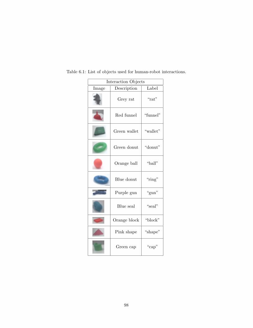
Table 6.1: List of objects used for human-robot interactions.
Interaction Objects
Image Description Label
Grey rat “rat”
Red funnel “funnel”
Green wallet “wallet”
Green donut “donut”
Orange ball “ball”
Blue donut “ring”
Purple gun “gun”
Blue seal “seal”
Orange block “block”
Pink shape “shape”
Green cap “cap”
98
first phase, the script was performed using only the first five objects in Table
6.1, while the other two (the blue donut and gun) were not yet present. Af-
ter sufficient training for the basic learning of these associations, the second
“phase” began, and the other two objects were introduced. The experiment
then proceeded in the same manner as before, with the exception that the
two new objects were now possible intentional targets within the script. The
purpose of this phase is to demonstrate the effective emergence of “lexical
contrast” principles within the pragmatic model. This is based on our intu-
ition that previous learning about word-meanings for the initial object set
will help to significantly improve intention inference and learning speed for
newly presented object-word pairs.
6.1.2 Implementation Details
The basic pragmatic model and learning algorithm outlined in Section 3.2,
along with the algorithms for construction of speech representations (Chap-
ter 4), and visual perception (Chapter 5) were implemented on the iCub
humanoid robot. The object segmentation and tracking algorithm produced
integer labels for each of the objects in the visual scene, which were used
as the set of possible intended referents for the tutor’s utterances. The rep-
resentation of words themselves were constructed using the sample imple-
mentation as was done for the action-word learning experiments presented
in Chapter 4. This included the transformation of the speech signal, first
into a 13-element MFCC feature vector, then into a sequence of phonetic
symbol probabilities, using the 10-state “phone” HMM, which were finally
used as inputs for the lexicon learning algorithm.
The other critical detail in the implementation of this experiment is the
use of gaze information, which we discussed in Section 3.2 to help shape
the prior over intents P (I|Z). The salience values zk from equation (5.13)
for each object are used to construct the prior probability for an intended
object given the gaze information:
P (I = k|Z) =zk + ε′∑k
zk′ + ε
. (6.1)
The “smoothing factor”, ε > 0, serves two purposes. The first is to ensure
that the prior P (I|Z) has full support of the entire set of I. This makes
proper inference of the intent using the complete posterior P (I|A,Z, φ) pos-
sible in cases where the gaze information is inaccurate, but the listener has
99
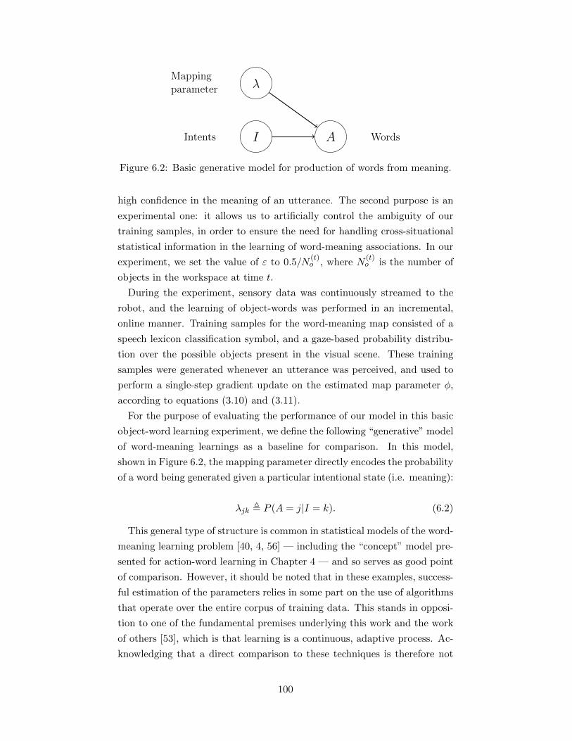
I A
λ
Intents Words
Mappingparameter
Figure 6.2: Basic generative model for production of words from meaning.
high confidence in the meaning of an utterance. The second purpose is an
experimental one: it allows us to artificially control the ambiguity of our
training samples, in order to ensure the need for handling cross-situational
statistical information in the learning of word-meaning associations. In our
experiment, we set the value of ε to 0.5/N(t)o , where N
(t)o is the number of
objects in the workspace at time t.
During the experiment, sensory data was continuously streamed to the
robot, and the learning of object-words was performed in an incremental,
online manner. Training samples for the word-meaning map consisted of a
speech lexicon classification symbol, and a gaze-based probability distribu-
tion over the possible objects present in the visual scene. These training
samples were generated whenever an utterance was perceived, and used to
perform a single-step gradient update on the estimated map parameter φ,
according to equations (3.10) and (3.11).
For the purpose of evaluating the performance of our model in this basic
object-word learning experiment, we define the following “generative” model
of word-meaning learnings as a baseline for comparison. In this model,
shown in Figure 6.2, the mapping parameter directly encodes the probability
of a word being generated given a particular intentional state (i.e. meaning):
λjk , P (A = j|I = k). (6.2)
This general type of structure is common in statistical models of the word-
meaning learning problem [40, 4, 56] — including the “concept” model pre-
sented for action-word learning in Chapter 4 — and so serves as good point
of comparison. However, it should be noted that in these examples, success-
ful estimation of the parameters relies in some part on the use of algorithms
that operate over the entire corpus of training data. This stands in opposi-
tion to one of the fundamental premises underlying this work and the work
of others [53], which is that learning is a continuous, adaptive process. Ac-
knowledging that a direct comparison to these techniques is therefore not
100
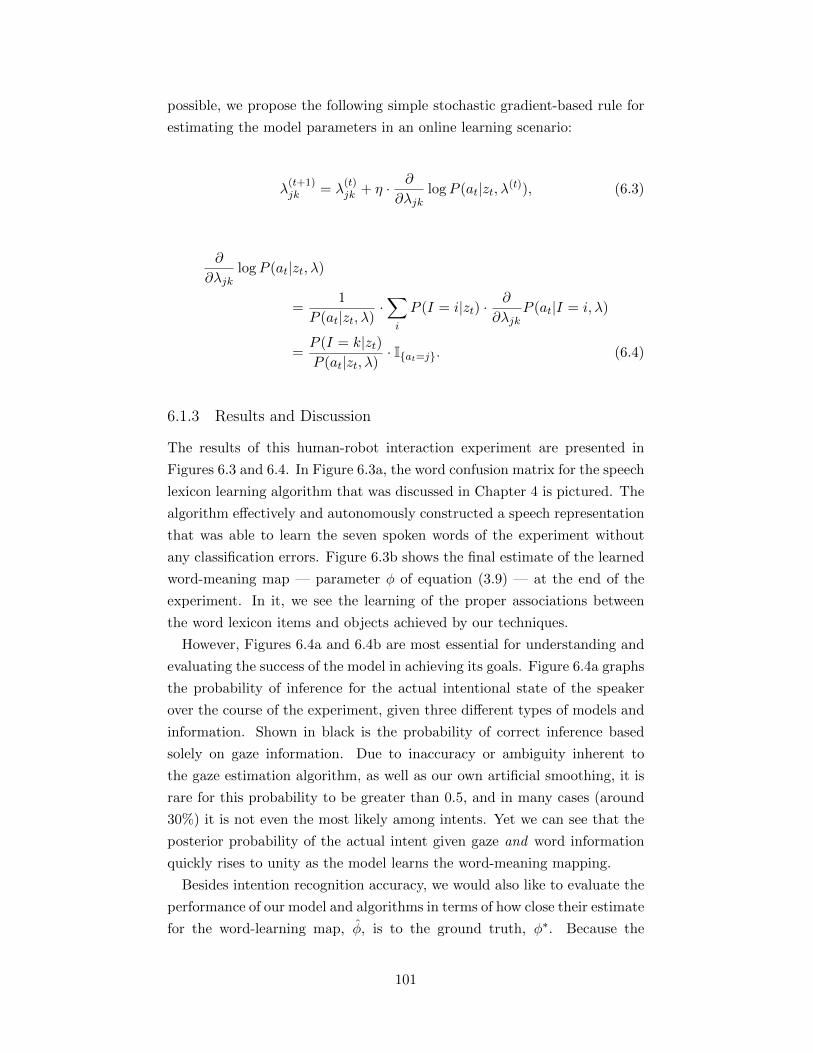
possible, we propose the following simple stochastic gradient-based rule for
estimating the model parameters in an online learning scenario:
λ(t+1)jk = λ
(t)jk + η · ∂
∂λjklogP (at|zt, λ(t)), (6.3)
∂
∂λjklogP (at|zt, λ)
=1
P (at|zt, λ)·∑i
P (I = i|zt) ·∂
∂λjkP (at|I = i, λ)
=P (I = k|zt)P (at|zt, λ)
· Iat=j. (6.4)
6.1.3 Results and Discussion
The results of this human-robot interaction experiment are presented in
Figures 6.3 and 6.4. In Figure 6.3a, the word confusion matrix for the speech
lexicon learning algorithm that was discussed in Chapter 4 is pictured. The
algorithm effectively and autonomously constructed a speech representation
that was able to learn the seven spoken words of the experiment without
any classification errors. Figure 6.3b shows the final estimate of the learned
word-meaning map — parameter φ of equation (3.9) — at the end of the
experiment. In it, we see the learning of the proper associations between
the word lexicon items and objects achieved by our techniques.
However, Figures 6.4a and 6.4b are most essential for understanding and
evaluating the success of the model in achieving its goals. Figure 6.4a graphs
the probability of inference for the actual intentional state of the speaker
over the course of the experiment, given three different types of models and
information. Shown in black is the probability of correct inference based
solely on gaze information. Due to inaccuracy or ambiguity inherent to
the gaze estimation algorithm, as well as our own artificial smoothing, it is
rare for this probability to be greater than 0.5, and in many cases (around
30%) it is not even the most likely among intents. Yet we can see that the
posterior probability of the actual intent given gaze and word information
quickly rises to unity as the model learns the word-meaning mapping.
Besides intention recognition accuracy, we would also like to evaluate the
performance of our model and algorithms in terms of how close their estimate
for the word-learning map, φ, is to the ground truth, φ∗. Because the
101
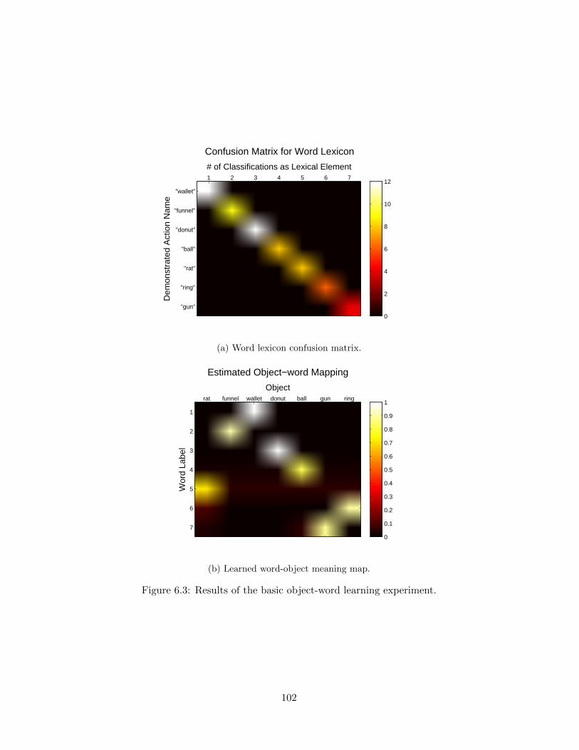
# of Classifications as Lexical Element
Confusion Matrix for Word Lexicon
Dem
onst
rate
d A
ctio
n N
ame
1 2 3 4 5 6 7
"wallet"
"funnel"
"donut"
"ball"
"rat"
"ring"
"gun"
0
2
4
6
8
10
12
(a) Word lexicon confusion matrix.
Object
Estimated Object−word Mapping
Wor
d La
bel
rat funnel wallet donut ball gun ring
1
2
3
4
5
6
7
0
0.1
0.2
0.3
0.4
0.5
0.6
0.7
0.8
0.9
1
(b) Learned word-object meaning map.
Figure 6.3: Results of the basic object-word learning experiment.
102
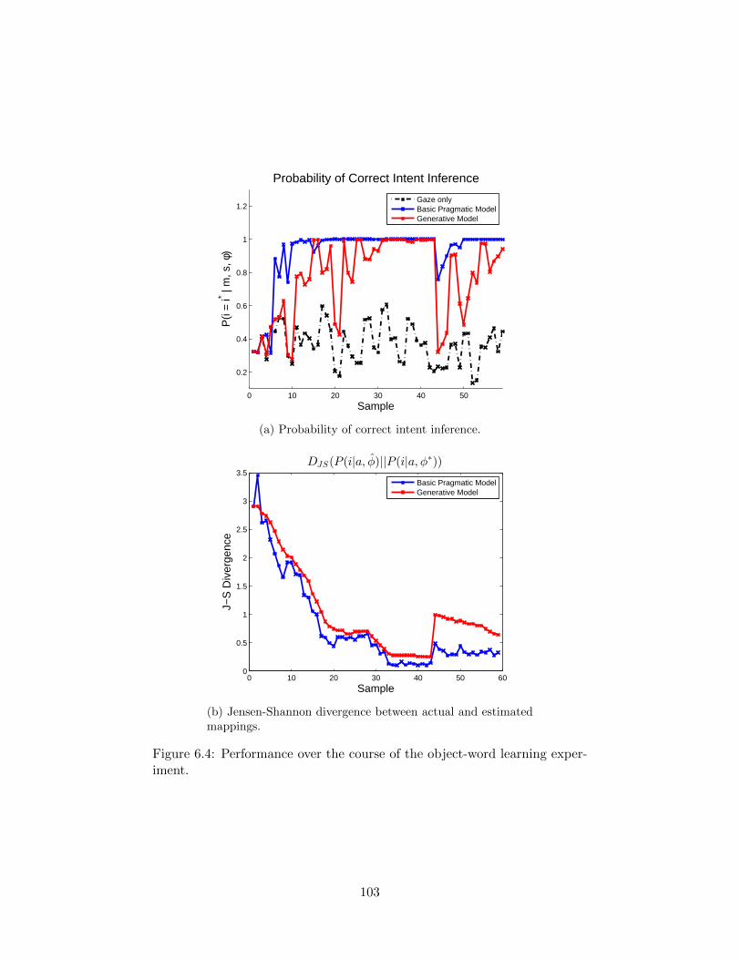
0 10 20 30 40 50
0.2
0.4
0.6
0.8
1
1.2
P(i
= i* |
m, s
, φ)
Sample
Probability of Correct Intent Inference
Gaze onlyBasic Pragmatic ModelGenerative Model
(a) Probability of correct intent inference.
0 10 20 30 40 50 600
0.5
1
1.5
2
2.5
3
3.5
J−S
Div
erge
nce
Sample
DJS(P(i|a, φ)||P(i|a,φ∗))
Basic Pragmatic ModelGenerative Model
(b) Jensen-Shannon divergence between actual and estimatedmappings.
Figure 6.4: Performance over the course of the object-word learning exper-iment.
103
parameters of the map represent a probability distribution over intents —
conditioned on a linguistic symbol — it may be useful for us to apply a
metric that measures the divergence between the estimated and ground-
truth distributions. For this purpose, we employ a divergence metric based
on the Jensen-Shannon divergence. The Jensen-Shannon divergence is a
symmetric divergence for probability distributions P and Q that is itself
based on the Kullback-Leibler divergence:
DJS(P ||Q) =1
2· [DKL(P ||(P +Q)/2) +DKL(Q||(P +Q)/2)] (6.5)
DKL(P ||Q) =∑i
Pi · logPiQi. (6.6)
We then define our derived distance metric as the following:
D(P (I|A, φ)||P (I|A, φ∗))
=1
Na
∑j
DJS(P (I|A = j, φ)||P (I|A = j, φ∗)). (6.7)
The divergence measure between the estimated and ground-truth maps
is pictured in Figure 6.4b. We can see that the model is able, for the most
part, to successfully learn the word-meaning map, in spite of significant
ambiguity, simply on the basis of statistical processing.
This steady convergence of our word-meaning map estimate is disrupted
in our experiment, however, when novel potential referents and words are
introduced. In these same two figures, we see that our baseline generative
model is able to do little better than gaze-only information when inferring
intent for a novel object-word pair, and as a result, is slow to learn map-
ping between these items. By comparison, the basic pragmatic model is
able to immediately resolve this ambiguity, by discounting possible targets
for which it has learned other words to be more effective communicators.
This allows the model to very quickly re-converge toward the correct word-
meaning parameter value. This capability is similar to that of the model
presented in [53], but in the case of our model, demonstration of the lex-
ical contrast principle is an emergent result of a more general ability for
pragmatic understanding of behavior.
104
6.2 Experiment II: Learning from Intentional Behavior
We now move on to the set of experiments for testing the aspects of our
model that constitute some of its most significant contributions. These are
the experiments in which our learner must learn and exploit knowledge about
the dual physical and communicative structure of the interaction in order to
resolve the tutor’s ambiguous linguistic references. In particular, we apply
the extended pragmatic model and algorithms presented in Section 3.3 to
a set of scenarios where the tutor is repeatedly performing some physical
task with a particular object, which is accompanied by a verbal description.
After learning a goal-centered representation of the task, our learning agent
is able to learn the meaning of the verbal descriptions, even in cases where
the physical component of the speaker’s behavior is incomplete, unsuccessful,
or otherwise ambiguous, in terms of its intended target.
6.2.1 Experiment IIa: Searching Game
The first of these experiments is built on the “searching game” of Tomasello,
Strosberg, and Akhtar [20]. In the original experiment, the adult tutor ver-
bally announced her intention to find a particular, novel object in a row of
buckets all containing such novel objects. The adult then began her search,
retrieving objects one by one, rejecting and replacing objects, until the in-
tended target was found. The episode concluded with the adult handing
the target object over to the child. The purpose of this experiment was to
demonstrate the inadequacy of basic attentional or saliency cues (e.g. the
adult’s temporally proximal interaction with an object) in resolving ambigu-
ity, and the necessity for the child to understand the entirety of the adult’s
behaviors in the context of the particular task (i.e. retrieval and hand-over).
For our purposes, we designed an experiment in the spirit of [20], but
with some major simplifications. As in the original, the procedure consisted
of a training phase where the task was introduced to the learner, and a
subsequent phase where language was used in conjunction with the searching
process detailed above. In the task training phase, the training episodes were
produced according to the following script:
1. Selection: The tutor selects one of the objects on the table as his/her
intended referent for the training episode.
2. Retrieval: The tutor reaches for the intended target object, grasps
it, and moves it to a location in front of himself/herself.
105
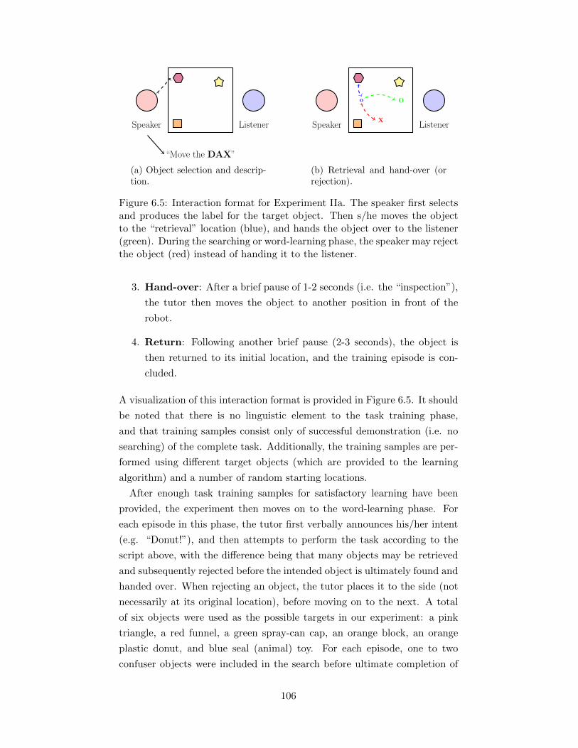
“Move the DAX”
Speaker Listener
(a) Object selection and descrip-tion.
Oo
XSpeaker Listener
(b) Retrieval and hand-over (orrejection).
Figure 6.5: Interaction format for Experiment IIa. The speaker first selectsand produces the label for the target object. Then s/he moves the objectto the “retrieval” location (blue), and hands the object over to the listener(green). During the searching or word-learning phase, the speaker may rejectthe object (red) instead of handing it to the listener.
3. Hand-over: After a brief pause of 1-2 seconds (i.e. the “inspection”),
the tutor then moves the object to another position in front of the
robot.
4. Return: Following another brief pause (2-3 seconds), the object is
then returned to its initial location, and the training episode is con-
cluded.
A visualization of this interaction format is provided in Figure 6.5. It should
be noted that there is no linguistic element to the task training phase,
and that training samples consist only of successful demonstration (i.e. no
searching) of the complete task. Additionally, the training samples are per-
formed using different target objects (which are provided to the learning
algorithm) and a number of random starting locations.
After enough task training samples for satisfactory learning have been
provided, the experiment then moves on to the word-learning phase. For
each episode in this phase, the tutor first verbally announces his/her intent
(e.g. “Donut!”), and then attempts to perform the task according to the
script above, with the difference being that many objects may be retrieved
and subsequently rejected before the intended object is ultimately found and
handed over. When rejecting an object, the tutor places it to the side (not
necessarily at its original location), before moving on to the next. A total
of six objects were used as the possible targets in our experiment: a pink
triangle, a red funnel, a green spray-can cap, an orange block, an orange
plastic donut, and blue seal (animal) toy. For each episode, one to two
confuser objects were included in the search before ultimate completion of
106
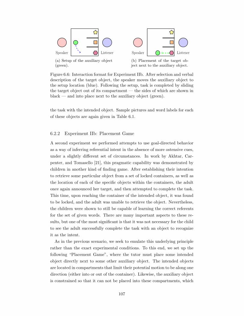
Speaker Listener
(a) Setup of the auxiliary object(green).
Speaker Listener
(b) Placement of the target ob-ject next to the auxiliary object.
Figure 6.6: Interaction format for Experiment IIb. After selection and verbaldescription of the target object, the speaker moves the auxiliary object tothe setup location (blue). Following the setup, task is completed by slidingthe target object out of its compartment — the sides of which are shown inblack — and into place next to the auxiliary object (green).
the task with the intended object. Sample pictures and word labels for each
of these objects are again given in Table 6.1.
6.2.2 Experiment IIb: Placement Game
A second experiment we performed attempts to use goal-directed behavior
as a way of inferring referential intent in the absence of more ostensive cues,
under a slightly different set of circumstances. In work by Akhtar, Car-
penter, and Tomasello [21], this pragmatic capability was demonstrated by
children in another kind of finding game. After establishing their intention
to retrieve some particular object from a set of locked containers, as well as
the location of each of the specific objects within the containers, the adult
once again announced her target, and then attempted to complete the task.
This time, upon reaching the container of the intended object, it was found
to be locked, and the adult was unable to retrieve the object. Nevertheless,
the children were shown to still be capable of learning the correct referents
for the set of given words. There are many important aspects to these re-
sults, but one of the most significant is that it was not necessary for the child
to see the adult successfully complete the task with an object to recognize
it as the intent.
As in the previous scenario, we seek to emulate this underlying principle
rather than the exact experimental conditions. To this end, we set up the
following “Placement Game”, where the tutor must place some intended
object directly next to some other auxiliary object. The intended objects
are located in compartments that limit their potential motion to be along one
direction (either into or out of the container). Likewise, the auxiliary object
is constrained so that it can not be placed into these compartments, which
107
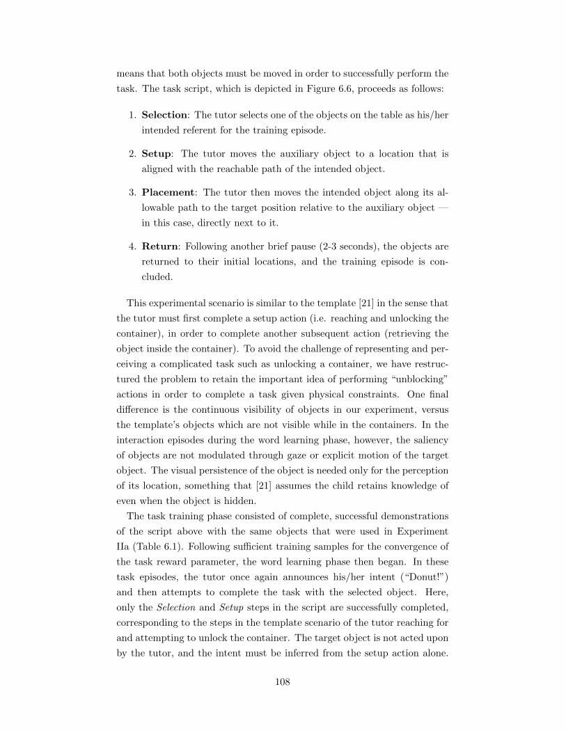
means that both objects must be moved in order to successfully perform the
task. The task script, which is depicted in Figure 6.6, proceeds as follows:
1. Selection: The tutor selects one of the objects on the table as his/her
intended referent for the training episode.
2. Setup: The tutor moves the auxiliary object to a location that is
aligned with the reachable path of the intended object.
3. Placement: The tutor then moves the intended object along its al-
lowable path to the target position relative to the auxiliary object —
in this case, directly next to it.
4. Return: Following another brief pause (2-3 seconds), the objects are
returned to their initial locations, and the training episode is con-
cluded.
This experimental scenario is similar to the template [21] in the sense that
the tutor must first complete a setup action (i.e. reaching and unlocking the
container), in order to complete another subsequent action (retrieving the
object inside the container). To avoid the challenge of representing and per-
ceiving a complicated task such as unlocking a container, we have restruc-
tured the problem to retain the important idea of performing “unblocking”
actions in order to complete a task given physical constraints. One final
difference is the continuous visibility of objects in our experiment, versus
the template’s objects which are not visible while in the containers. In the
interaction episodes during the word learning phase, however, the saliency
of objects are not modulated through gaze or explicit motion of the target
object. The visual persistence of the object is needed only for the perception
of its location, something that [21] assumes the child retains knowledge of
even when the object is hidden.
The task training phase consisted of complete, successful demonstrations
of the script above with the same objects that were used in Experiment
IIa (Table 6.1). Following sufficient training samples for the convergence of
the task reward parameter, the word learning phase then began. In these
task episodes, the tutor once again announces his/her intent (“Donut!”)
and then attempts to complete the task with the selected object. Here,
only the Selection and Setup steps in the script are successfully completed,
corresponding to the steps in the template scenario of the tutor reaching for
and attempting to unlock the container. The target object is not acted upon
by the tutor, and the intent must be inferred from the setup action alone.
108
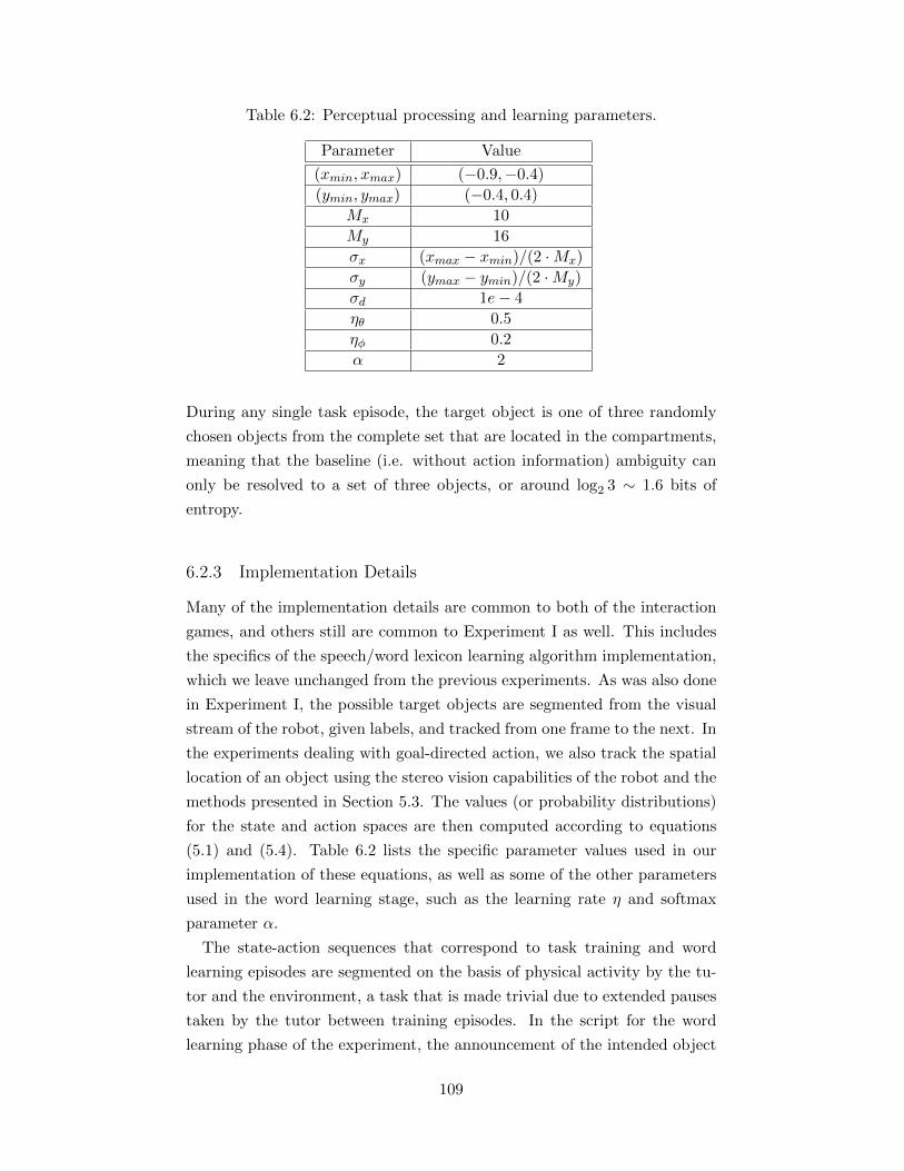
Table 6.2: Perceptual processing and learning parameters.
Parameter Value
(xmin, xmax) (−0.9,−0.4)
(ymin, ymax) (−0.4, 0.4)
Mx 10
My 16
σx (xmax − xmin)/(2 ·Mx)
σy (ymax − ymin)/(2 ·My)
σd 1e− 4
ηθ 0.5
ηφ 0.2
α 2
During any single task episode, the target object is one of three randomly
chosen objects from the complete set that are located in the compartments,
meaning that the baseline (i.e. without action information) ambiguity can
only be resolved to a set of three objects, or around log2 3 ∼ 1.6 bits of
entropy.
6.2.3 Implementation Details
Many of the implementation details are common to both of the interaction
games, and others still are common to Experiment I as well. This includes
the specifics of the speech/word lexicon learning algorithm implementation,
which we leave unchanged from the previous experiments. As was also done
in Experiment I, the possible target objects are segmented from the visual
stream of the robot, given labels, and tracked from one frame to the next. In
the experiments dealing with goal-directed action, we also track the spatial
location of an object using the stereo vision capabilities of the robot and the
methods presented in Section 5.3. The values (or probability distributions)
for the state and action spaces are then computed according to equations
(5.1) and (5.4). Table 6.2 lists the specific parameter values used in our
implementation of these equations, as well as some of the other parameters
used in the word learning stage, such as the learning rate η and softmax
parameter α.
The state-action sequences that correspond to task training and word
learning episodes are segmented on the basis of physical activity by the tu-
tor and the environment, a task that is made trivial due to extended pauses
taken by the tutor between training episodes. In the script for the word
learning phase of the experiment, the announcement of the intended object
109
always precedes the demonstration of goal-directed action. Therefore, when
an utterance is heard and corresponding word symbol, mt ∈ Am, is gener-
ated, this is matched with the next state-action sequence to be observed,
and used as a training sample, (mt, st, atTt=0).
Between the two experiments explored in this section, there are a number
of relatively minor implementation differences, mostly in the specifics of the
task features and parameterization, as well as physical constraints on action
that are imposed through the state-action transition model.
Experiment IIa Details
For the Searching Game, there are no special considerations for the tran-
sition model T beyond what is detailed in Section 5.2. Likewise, we use a
straightforward set of features for each state, where the vector produced by
the feature-generating function ψ : S → Rf is of length f = |S|, and has
a value of 0 for all but the s-th element, which has value 1. As mentioned
previously, this means that each element of θ effectively encodes the exact
value of the reward function for each state in the (reduced) state-space. This
reduced state space is transformed from the complete state-space by intent-
dependent mapping gi(s), which simply selects the individual state-space
corresponding to object i.
Experiment IIb Details
Experiment IIb requires a slightly different and more complex implementa-
tion for many of these components. We begin with gi(s), which reduces Sto a space composed of the intended object’s state, as well as the state of
the auxiliary object: S = Si × Saux. The function hi(a) transforms to a
similarly composed set of actions. The state-action transition model T is
defined such that the intended objects may not be moved laterally (in the Y
direction of the root frame) due to the constraints of the compartments, and
the auxiliary object may not be moved past the X locations (X > −0.6m)
at which the compartments begin. Finally, we define the feature vector ψ(s)
as the concatenation of three smaller feature vectors. The first two are the
same state-selector type of features used above, for both the intended and
auxiliary objects’ state spaces. The third is also a 0/1-valued vector corre-
sponding to the relative distance between the two objects with respect to
their locations on the spatial grid.
110
6.2.4 Results and Discussion
Both of the experiments presented in this section consist of two general
phases: a task learning phase aimed at learning the intent-independent
aspects of the physical task, and a word-learning phase, where a verbal
description is provided alongside an incomplete, unsuccessful, or otherwise
ambiguous attempt to perform the task using the specific object of reference.
Here, we present the results of the task training, as well as demonstrations
of the successful inference of intent from goal-directed behaviors, for each of
the two experimental scenarios. We then use the results of the word-learning
episodes from both to learn a single word-meaning mapping.
Experiment IIa Results and Discussion
The results of the task training phase for the Searching Game are presented
in Figure 6.7. Three training samples (Figure 6.7a) were presented, and
three of the gradient steps of equation (3.28) were taken for each demon-
stration. Figure 6.7b shows the estimated task parameters as the vector of
feature weights, while Figure 6.7c displays it according to the reward value
at each location of the state-space grid. From these, we can see that the
reward function is nearly zero at all states, except for a small few, which
correspond to the two locations where the tutor moves the objects during
the retrieval and hand-over steps of the script. These invariances of the task
are captured by the IRL algorithm, even under the variations in starting
point and path of movement across the training observations.
The training episodes during the word-learning phase consisted of a series
of movements of various objects toward the “retrieval” position, followed by
either a rejection (not-intended), or a hand-over (intended) of the object, the
latter of which concludes the training episode. In order to properly use the
observed behavior to resolve ambiguity for word learning, the goal-centered
(intentional) model is essential. Consider the data from an sample episode
shown in Figure 6.8. In this example, cues such as motion salience of an
object will be ambiguous (as three objects are moving over the course of
the episode), while others, such as temporal synchrony, will be inaccurate
(Objects 4 and 6 are moved prior to Object 2, which is the intended object).
Direct models of trajectory, such as the HMM-based representation used
in [87] and our own work in Chapter 4, will also be inadequate, given the
variations in position and path seen in Figure 6.8a.
Figure 6.8b shows how the goal-based representation of behavior is able to
111
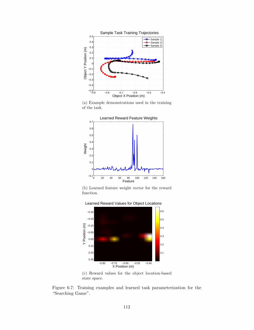
−0.9 −0.8 −0.7 −0.6 −0.5 −0.4−0.5
−0.4
−0.3
−0.2
−0.1
0
0.1
0.2
0.3
0.4
0.5
Object X Position (m)
Sample Task Training Trajectories
Obj
ect Y
Pos
ition
(m
)
Sample 1Sample 2Sample 3
(a) Example demonstrations used in the trainingof the task.
0 20 40 60 80 100 120 140 160−0.1
0
0.1
0.2
0.3
0.4
0.5
0.6
0.7
Wei
ght
Feature
Learned Reward Feature Weights
(b) Learned feature weight vector for the rewardfunction.
Y P
ositi
on (
m)
X Position (m)
Learned Reward Values for Object Locations
−0.85 −0.75 −0.65 −0.55 −0.45
−0.35
−0.25
−0.15
−0.05
0.05
0.15
0.25
0.35
0.1
0.2
0.3
0.4
0.5
0.6
(c) Reward values for the object location-basedstate space.
Figure 6.7: Training examples and learned task parameterization for the“Searching Game”.
112
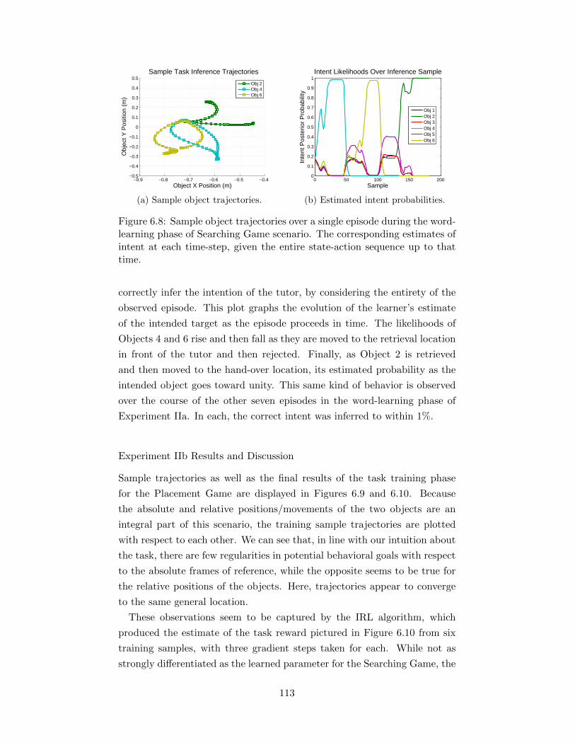
−0.9 −0.8 −0.7 −0.6 −0.5 −0.4−0.5
−0.4
−0.3
−0.2
−0.1
0
0.1
0.2
0.3
0.4
0.5
Object X Position (m)
Sample Task Inference Trajectories
Obj
ect Y
Pos
ition
(m
)
Obj 2Obj 4Obj 6
(a) Sample object trajectories.
0 50 100 150 2000
0.1
0.2
0.3
0.4
0.5
0.6
0.7
0.8
0.9
1
Inte
nt P
oste
rior
Pro
babi
lity
Sample
Intent Likelihoods Over Inference Sample
Obj 1Obj 2Obj 3Obj 4Obj 5Obj 6
(b) Estimated intent probabilities.
Figure 6.8: Sample object trajectories over a single episode during the word-learning phase of Searching Game scenario. The corresponding estimates ofintent at each time-step, given the entire state-action sequence up to thattime.
correctly infer the intention of the tutor, by considering the entirety of the
observed episode. This plot graphs the evolution of the learner’s estimate
of the intended target as the episode proceeds in time. The likelihoods of
Objects 4 and 6 rise and then fall as they are moved to the retrieval location
in front of the tutor and then rejected. Finally, as Object 2 is retrieved
and then moved to the hand-over location, its estimated probability as the
intended object goes toward unity. This same kind of behavior is observed
over the course of the other seven episodes in the word-learning phase of
Experiment IIa. In each, the correct intent was inferred to within 1%.
Experiment IIb Results and Discussion
Sample trajectories as well as the final results of the task training phase
for the Placement Game are displayed in Figures 6.9 and 6.10. Because
the absolute and relative positions/movements of the two objects are an
integral part of this scenario, the training sample trajectories are plotted
with respect to each other. We can see that, in line with our intuition about
the task, there are few regularities in potential behavioral goals with respect
to the absolute frames of reference, while the opposite seems to be true for
the relative positions of the objects. Here, trajectories appear to converge
to the same general location.
These observations seem to be captured by the IRL algorithm, which
produced the estimate of the task reward pictured in Figure 6.10 from six
training samples, with three gradient steps taken for each. While not as
strongly differentiated as the learned parameter for the Searching Game, the
113
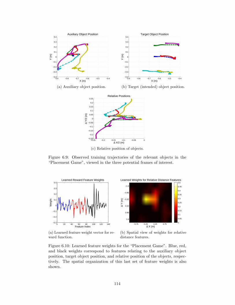
−0.9 −0.8 −0.7 −0.6 −0.5 −0.4−0.4
−0.3
−0.2
−0.1
0
0.1
0.2
0.3
0.4
X (m)
Y (
m)
Auxiliary Object Position
(a) Auxiliary object position.
−0.9 −0.8 −0.7 −0.6 −0.5 −0.4−0.4
−0.3
−0.2
−0.1
0
0.1
0.2
0.3
0.4
X (m)
Y (
m)
Target Object Position
(b) Target (intended) object position.
−0.25 −0.2 −0.15 −0.1 −0.05 0−0.25
−0.2
−0.15
−0.1
−0.05
0
0.05
0.1
0.15
0.2
0.25
∆ X/2 (m)
∆ Y
/2 (
m)
Relative Positions
(c) Relative position of objects.
Figure 6.9: Observed training trajectories of the relevant objects in the“Placement Game”, viewed in the three potential frames of interest.
0 20 40 60 80 100 120 140−0.3
−0.2
−0.1
0
0.1
0.2
0.3
0.4
Feature Index
Wei
ght
Learned Reward Feature Weights
(a) Learned feature weight vector for re-ward function.
∆ X (m)
∆ Y
(m
)
Learned Weights for Relative Distance Features
−0.75 −0.25 0.25 0.75
−1.6
−0.96
−0.32
0.32
0.96
1.6
0
0.05
0.1
0.15
0.2
0.25
0.3
0.35
0.4
0.45
0.5
(b) Spatial view of weights for relativedistance features.
Figure 6.10: Learned feature weights for the “Placement Game”. Blue, red,and black weights correspond to features relating to the auxiliary objectposition, target object position, and relative position of the objects, respec-tively. The spatial organization of this last set of feature weights is alsoshown.
114
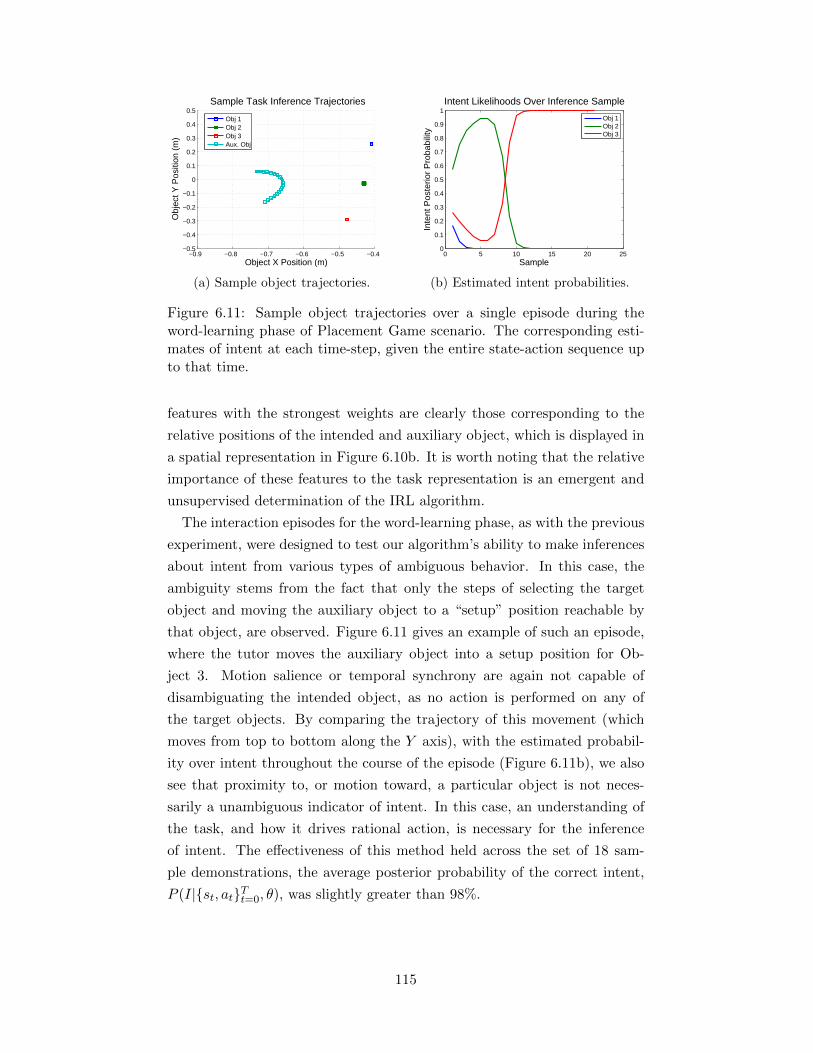
−0.9 −0.8 −0.7 −0.6 −0.5 −0.4−0.5
−0.4
−0.3
−0.2
−0.1
0
0.1
0.2
0.3
0.4
0.5
Object X Position (m)
Sample Task Inference Trajectories
Obj
ect Y
Pos
ition
(m
)
Obj 1Obj 2Obj 3Aux. Obj
(a) Sample object trajectories.
0 5 10 15 20 250
0.1
0.2
0.3
0.4
0.5
0.6
0.7
0.8
0.9
1
Inte
nt P
oste
rior
Pro
babi
lity
Sample
Intent Likelihoods Over Inference Sample
Obj 1Obj 2Obj 3
(b) Estimated intent probabilities.
Figure 6.11: Sample object trajectories over a single episode during theword-learning phase of Placement Game scenario. The corresponding esti-mates of intent at each time-step, given the entire state-action sequence upto that time.
features with the strongest weights are clearly those corresponding to the
relative positions of the intended and auxiliary object, which is displayed in
a spatial representation in Figure 6.10b. It is worth noting that the relative
importance of these features to the task representation is an emergent and
unsupervised determination of the IRL algorithm.
The interaction episodes for the word-learning phase, as with the previous
experiment, were designed to test our algorithm’s ability to make inferences
about intent from various types of ambiguous behavior. In this case, the
ambiguity stems from the fact that only the steps of selecting the target
object and moving the auxiliary object to a “setup” position reachable by
that object, are observed. Figure 6.11 gives an example of such an episode,
where the tutor moves the auxiliary object into a setup position for Ob-
ject 3. Motion salience or temporal synchrony are again not capable of
disambiguating the intended object, as no action is performed on any of
the target objects. By comparing the trajectory of this movement (which
moves from top to bottom along the Y axis), with the estimated probabil-
ity over intent throughout the course of the episode (Figure 6.11b), we also
see that proximity to, or motion toward, a particular object is not neces-
sarily a unambiguous indicator of intent. In this case, an understanding of
the task, and how it drives rational action, is necessary for the inference
of intent. The effectiveness of this method held across the set of 18 sam-
ple demonstrations, the average posterior probability of the correct intent,
P (I|st, atTt=0, θ), was slightly greater than 98%.
115
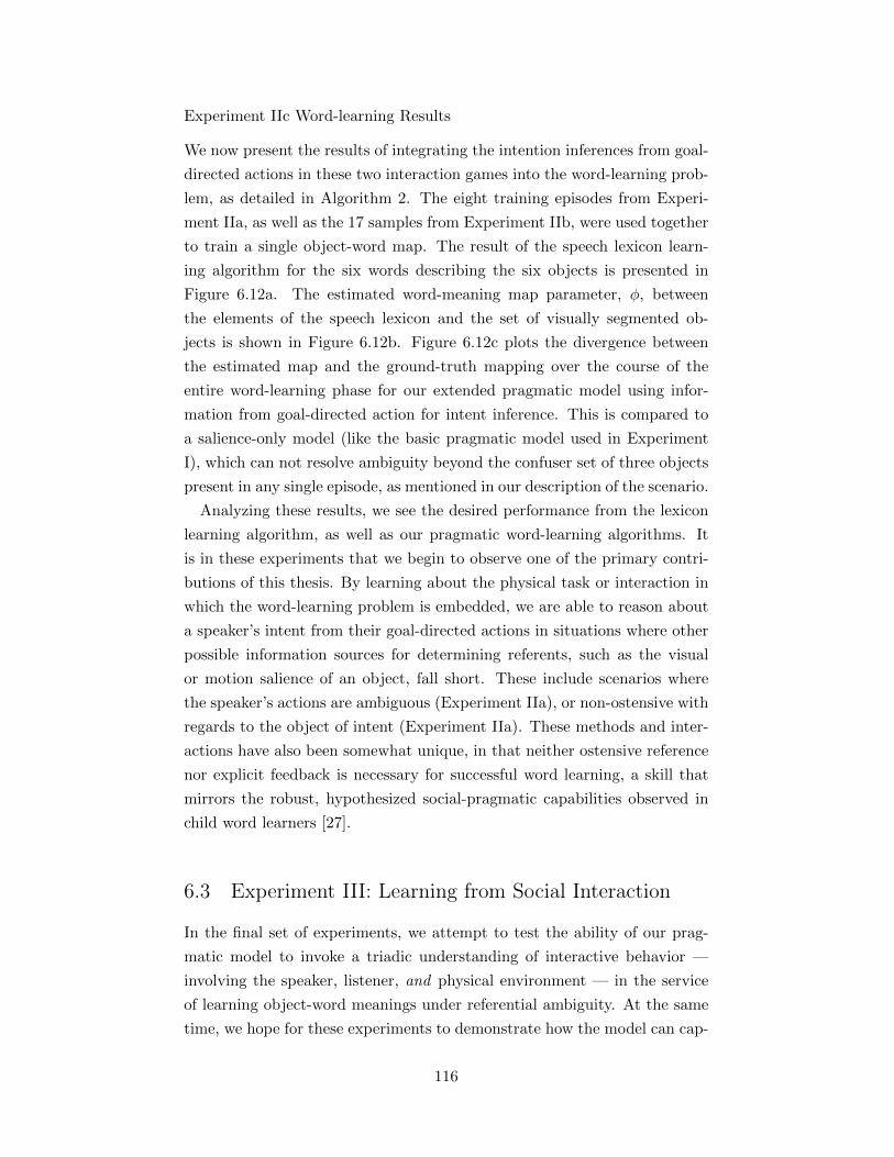
Experiment IIc Word-learning Results
We now present the results of integrating the intention inferences from goal-
directed actions in these two interaction games into the word-learning prob-
lem, as detailed in Algorithm 2. The eight training episodes from Experi-
ment IIa, as well as the 17 samples from Experiment IIb, were used together
to train a single object-word map. The result of the speech lexicon learn-
ing algorithm for the six words describing the six objects is presented in
Figure 6.12a. The estimated word-meaning map parameter, φ, between
the elements of the speech lexicon and the set of visually segmented ob-
jects is shown in Figure 6.12b. Figure 6.12c plots the divergence between
the estimated map and the ground-truth mapping over the course of the
entire word-learning phase for our extended pragmatic model using infor-
mation from goal-directed action for intent inference. This is compared to
a salience-only model (like the basic pragmatic model used in Experiment
I), which can not resolve ambiguity beyond the confuser set of three objects
present in any single episode, as mentioned in our description of the scenario.
Analyzing these results, we see the desired performance from the lexicon
learning algorithm, as well as our pragmatic word-learning algorithms. It
is in these experiments that we begin to observe one of the primary contri-
butions of this thesis. By learning about the physical task or interaction in
which the word-learning problem is embedded, we are able to reason about
a speaker’s intent from their goal-directed actions in situations where other
possible information sources for determining referents, such as the visual
or motion salience of an object, fall short. These include scenarios where
the speaker’s actions are ambiguous (Experiment IIa), or non-ostensive with
regards to the object of intent (Experiment IIa). These methods and inter-
actions have also been somewhat unique, in that neither ostensive reference
nor explicit feedback is necessary for successful word learning, a skill that
mirrors the robust, hypothesized social-pragmatic capabilities observed in
child word learners [27].
6.3 Experiment III: Learning from Social Interaction
In the final set of experiments, we attempt to test the ability of our prag-
matic model to invoke a triadic understanding of interactive behavior —
involving the speaker, listener, and physical environment — in the service
of learning object-word meanings under referential ambiguity. At the same
time, we hope for these experiments to demonstrate how the model can cap-
116
# of Classifications as Lexical Element
Confusion Matrix for Word Lexicon
Spo
ken
Wor
d
1 2 3 4 5 6
shape
seal
block
donut
cap
funnel
0
1
2
3
4
5
6
7
(a) Confusion matrix for learned speech lexicon.
Object
Estimated Object−word Mapping
Wor
d La
bel
1 2 3 4 5 6
1
2
3
4
5
6
0
0.1
0.2
0.3
0.4
0.5
0.6
0.7
0.8
0.9
1
(b) Learned object-word meaning map.
0 5 10 15 20 250
0.05
0.1
0.15
0.2
0.25
0.3
0.35
0.4
0.45
J−S
Div
erge
nce
Sample
DJS(P(i|a, φ)||P(i|a,φ∗))
Pragmatic InferenceSaliency Only
(c) Jensen-Shannon divergence between estimatedand ground-truth object-word meaning map overcourse of training.
Figure 6.12: Results of combined experiment for word-learning from under-standing of goal-directed behavior.
117
ture pragmatic meaning that extends beyond simple reference to an object,
and into a request for a joint action between speaker and listener upon that
object, framed by the context of the learned interaction. Finally, we show
how the representation of the learner’s own ability to take action, embedded
in the triadic model, allows the listener to become an active participant in
the task, and to improve the process of word-learning.
The scenario for this set of experiments is based on the interactions pre-
sented in [75, 24], where a speaker is attempting to complete some task in
the presence of a listener. The key feature to these scenarios are the loca-
tions of various objects, potentially to be used in the task, in one of two
distinct physical spaces. These are the “Speaker’s” and the “Listener’s”
areas, which designate the object locations that the speaker and listener, re-
spectively, are capable of reaching. During the interaction, when the listener
hears a verbal request for an object, s/he will favor intentional inferences for
objects in areas reachable to himself/herself, and not to the speaker. Under
a pragmatic view, objects that are reachable by the speaker are discounted
by reasoning that the speaker would have had better chances of completing
the task simply by acting his/herself, rather than enlisting the aid of the lis-
tener. This requires the listener to exploit knowledge of the task structure,
the action constraints of both agents, as well as linguistic conventions. As
we mentioned previously, the experiments in [75, 24] do not explicitly deal
with the problem of word learning, but we use their fundamental focus on
pragmatic resolution of referential ambiguity for the purposes of our own
word-learning experiments.
6.3.1 Scenario and Setup
The setup of our interaction scenario bears similarities to both our previous
interactions, as well as these new template experiments. As before, the
environment consists of a human tutor and robot learner, seated at a table
upon which many objects have been placed. Conceptually, the table has two
regions, corresponding to the locations that are reachable/unreachable to the
tutor, the boundaries of which we assume to be known to our learning agent.
We consider all areas of the work space to be reachable to this learner. The
objects in this experiment are reused from the previous two experiments:
a plastic donut, funnel, wallet, seal toy, ceramic mug, and a plastic block.
The task to be completed, however, was simpler in comparison, and involved
only the movement of a selected object to a particular location in front of
the tutor. The interaction for task training was performed according to this
118
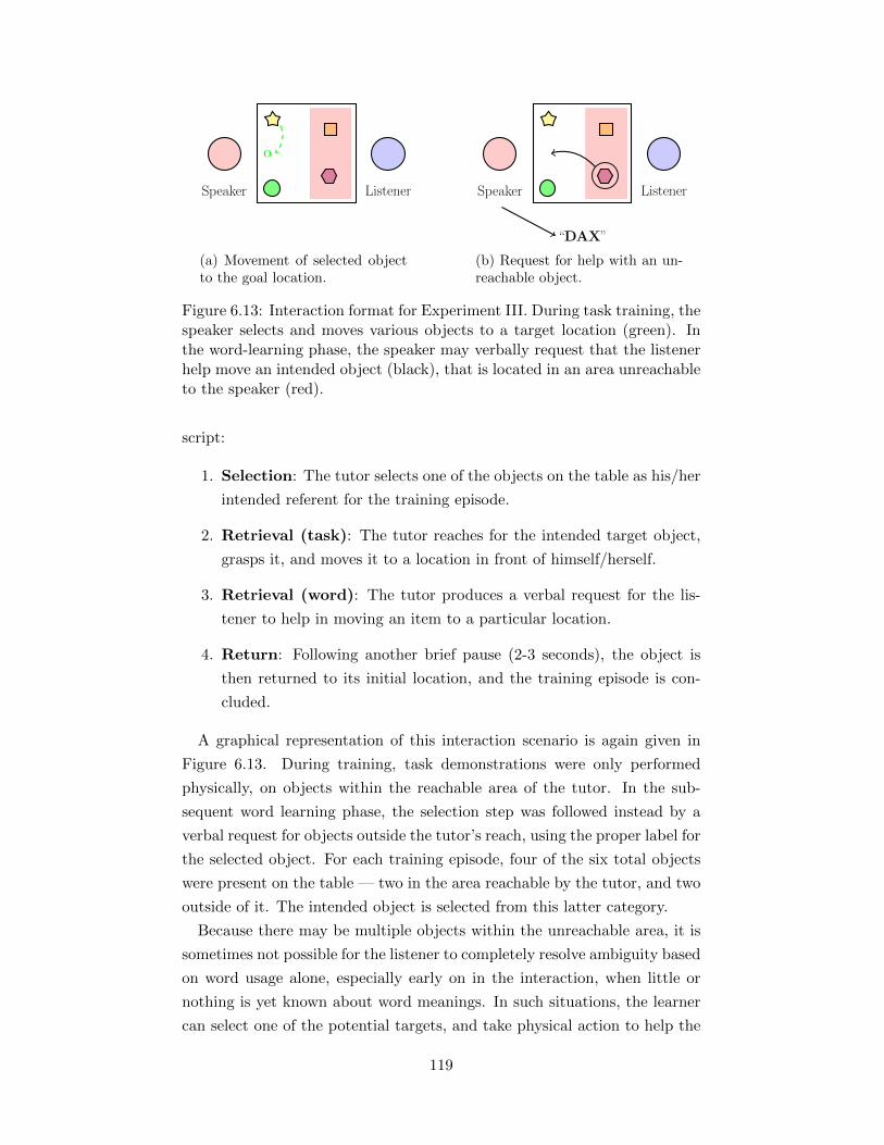
O
Speaker Listener
(a) Movement of selected objectto the goal location.
“DAX”
Speaker Listener
(b) Request for help with an un-reachable object.
Figure 6.13: Interaction format for Experiment III. During task training, thespeaker selects and moves various objects to a target location (green). Inthe word-learning phase, the speaker may verbally request that the listenerhelp move an intended object (black), that is located in an area unreachableto the speaker (red).
script:
1. Selection: The tutor selects one of the objects on the table as his/her
intended referent for the training episode.
2. Retrieval (task): The tutor reaches for the intended target object,
grasps it, and moves it to a location in front of himself/herself.
3. Retrieval (word): The tutor produces a verbal request for the lis-
tener to help in moving an item to a particular location.
4. Return: Following another brief pause (2-3 seconds), the object is
then returned to its initial location, and the training episode is con-
cluded.
A graphical representation of this interaction scenario is again given in
Figure 6.13. During training, task demonstrations were only performed
physically, on objects within the reachable area of the tutor. In the sub-
sequent word learning phase, the selection step was followed instead by a
verbal request for objects outside the tutor’s reach, using the proper label for
the selected object. For each training episode, four of the six total objects
were present on the table — two in the area reachable by the tutor, and two
outside of it. The intended object is selected from this latter category.
Because there may be multiple objects within the unreachable area, it is
sometimes not possible for the listener to completely resolve ambiguity based
on word usage alone, especially early on in the interaction, when little or
nothing is yet known about word meanings. In such situations, the learner
can select one of the potential targets, and take physical action to help the
119
speaker achieve the task with the intended target. Then using the reaction
of the tutor, the learner could update its estimate of intent, according to
the methods detailed in Algorithm 3. In our experiment, the speaker either
reacts by renewing his/her request for the object (implying that the guess
of the robot was not correct), or by acting to complete the task with the
intended object now in the reachable area.
6.3.2 Implementation Details
The implementation of the computational and perceptual processes for this
experiment was mostly the same as that used previously for Experiment IIa,
but with a few important changes and additions. As noted in Section 3.4
and Algorithm 3, the learning agent must retain optimal Q-functions under
the task parameter θ for both itself and the speaker. In the current scenario,
we embed the action constraints on the speaker in the stochastic state-action
transition model T σ by setting the probabilities of all self-transitions to 1 for
states corresponding to objects located in the half of the table nearest to the
robot (X > −0.6). Because of the need for a larger model of the workspace
in order to accommodate the different regions of allowable movements for the
tutor, the spatial processing parameters for the limits on the X dimension
were changed to xmin = −1.1 m and xmax = −0.45 m.
The extension of this experiment allows the robot to join in the task in
order to get feedback from the speaker if it determines its uncertainty about
the intended referent to be significant enough. We use a value of 1 bit of
entropy over P (I|S,Am, θ, φ) as the threshold for choosing whether to make
such an action. Ideally, if the robot decided to take action, it would generate
such actions according to lines 10-13 in Algorithm 3. For our specific exper-
iment, where there are no constraints on the robot’s movements in the task
space, the optimal movement trajectory is simply a straight line between
the target object’s current location and the goal location. Because of this,
the control of the action sequence performed by the robot was implemented
using the actionPrimitives and Cartesian Controller [127] modules available
in the iCub’s open-source code library. These allow us to command the
robot to move its arm to the particular location of the object, grasp the
object, move it to the goal location, and finally release the object. In order
to maintain proper function and persistence of the visually tracked objects
while the robot is completing this motion — which often causes objects to
go out of view due to rotation of the torso — the segmentation and tracking
algorithm is paused for the duration of the action.
120
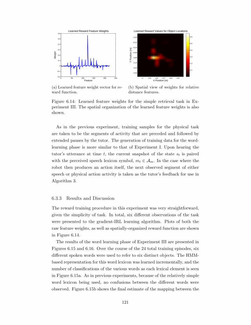
0 50 100 150 200 250−0.2
−0.1
0
0.1
0.2
0.3
0.4
0.5
0.6
Wei
ght
Feature
Learned Reward Feature Weights
(a) Learned feature weight vector for re-ward function.
Y P
ositi
on (
m)
X Position (m)
Learned Reward Values for Object Locations
−1 −0.9 −0.8 −0.7 −0.6 −0.5
−0.35
−0.25
−0.15
−0.05
0.05
0.15
0.25
0.35
0.1
0.2
0.3
0.4
0.5
0.6
(b) Spatial view of weights for relativedistance features.
Figure 6.14: Learned feature weights for the simple retrieval task in Ex-periment III. The spatial organization of the learned feature weights is alsoshown.
As in the previous experiment, training samples for the physical task
are taken to be the segments of activity that are preceded and followed by
extended pauses by the tutor. The generation of training data for the word-
learning phase is more similar to that of Experiment I. Upon hearing the
tutor’s utterance at time t, the current snapshot of the state st is paired
with the perceived speech lexicon symbol, mt ∈ Am. In the case where the
robot then produces an action itself, the next observed segment of either
speech or physical action activity is taken as the tutor’s feedback for use in
Algorithm 3.
6.3.3 Results and Discussion
The reward training procedure in this experiment was very straightforward,
given the simplicity of task. In total, six different observations of the task
were presented to the gradient-IRL learning algorithm. Plots of both the
raw feature weights, as well as spatially-organized reward function are shown
in Figure 6.14.
The results of the word learning phase of Experiment III are presented in
Figures 6.15 and 6.16. Over the course of the 24 total training episodes, six
different spoken words were used to refer to six distinct objects. The HMM-
based representation for this word lexicon was learned incrementally, and the
number of classifications of the various words as each lexical element is seen
in Figure 6.15a. As in previous experiments, because of the relatively simple
word lexicon being used, no confusions between the different words were
observed. Figure 6.15b shows the final estimate of the mapping between the
121
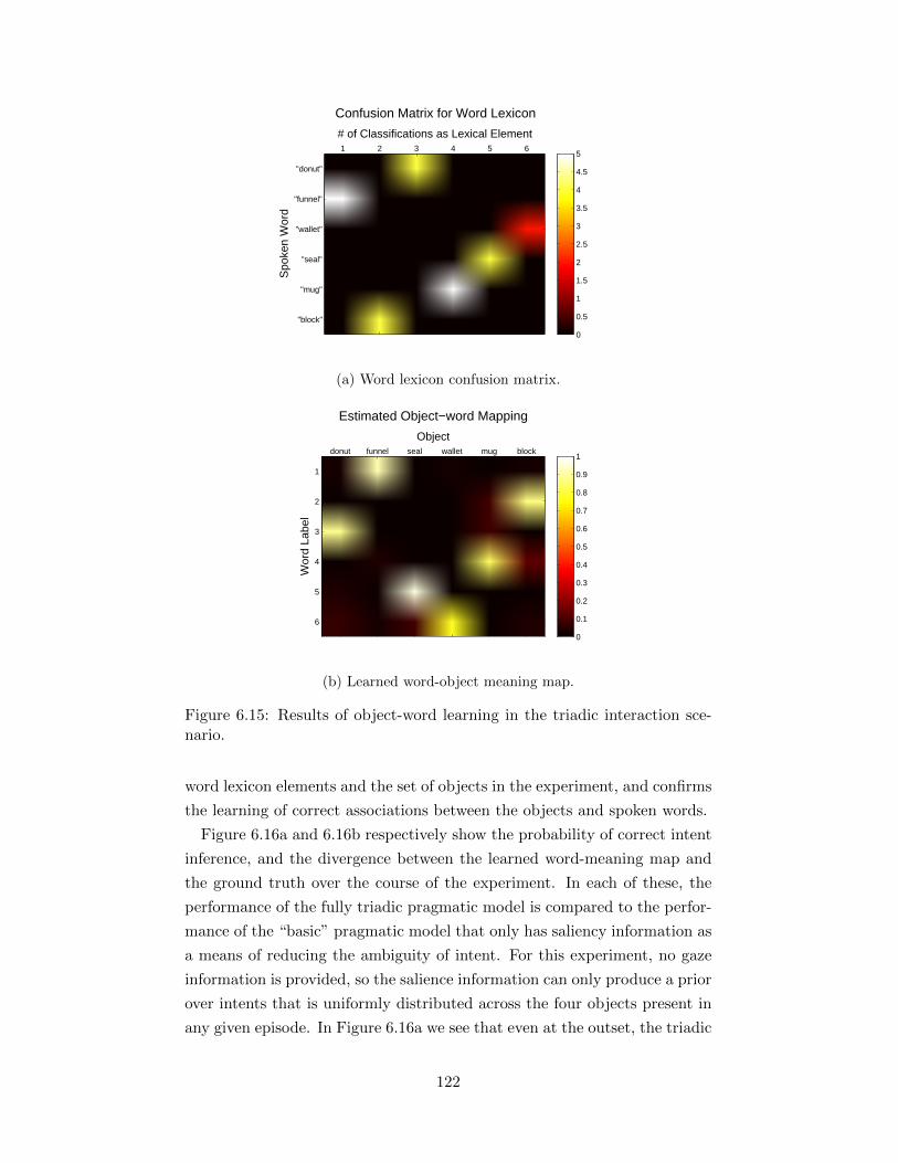
# of Classifications as Lexical Element
Confusion Matrix for Word Lexicon
Spo
ken
Wor
d
1 2 3 4 5 6
"donut"
"funnel"
"wallet"
"seal"
"mug"
"block"
0
0.5
1
1.5
2
2.5
3
3.5
4
4.5
5
(a) Word lexicon confusion matrix.
Object
Estimated Object−word Mapping
Wor
d La
bel
donut funnel seal wallet mug block
1
2
3
4
5
6
0
0.1
0.2
0.3
0.4
0.5
0.6
0.7
0.8
0.9
1
(b) Learned word-object meaning map.
Figure 6.15: Results of object-word learning in the triadic interaction sce-nario.
word lexicon elements and the set of objects in the experiment, and confirms
the learning of correct associations between the objects and spoken words.
Figure 6.16a and 6.16b respectively show the probability of correct intent
inference, and the divergence between the learned word-meaning map and
the ground truth over the course of the experiment. In each of these, the
performance of the fully triadic pragmatic model is compared to the perfor-
mance of the “basic” pragmatic model that only has saliency information as
a means of reducing the ambiguity of intent. For this experiment, no gaze
information is provided, so the salience information can only produce a prior
over intents that is uniformly distributed across the four objects present in
any given episode. In Figure 6.16a we see that even at the outset, the triadic
122
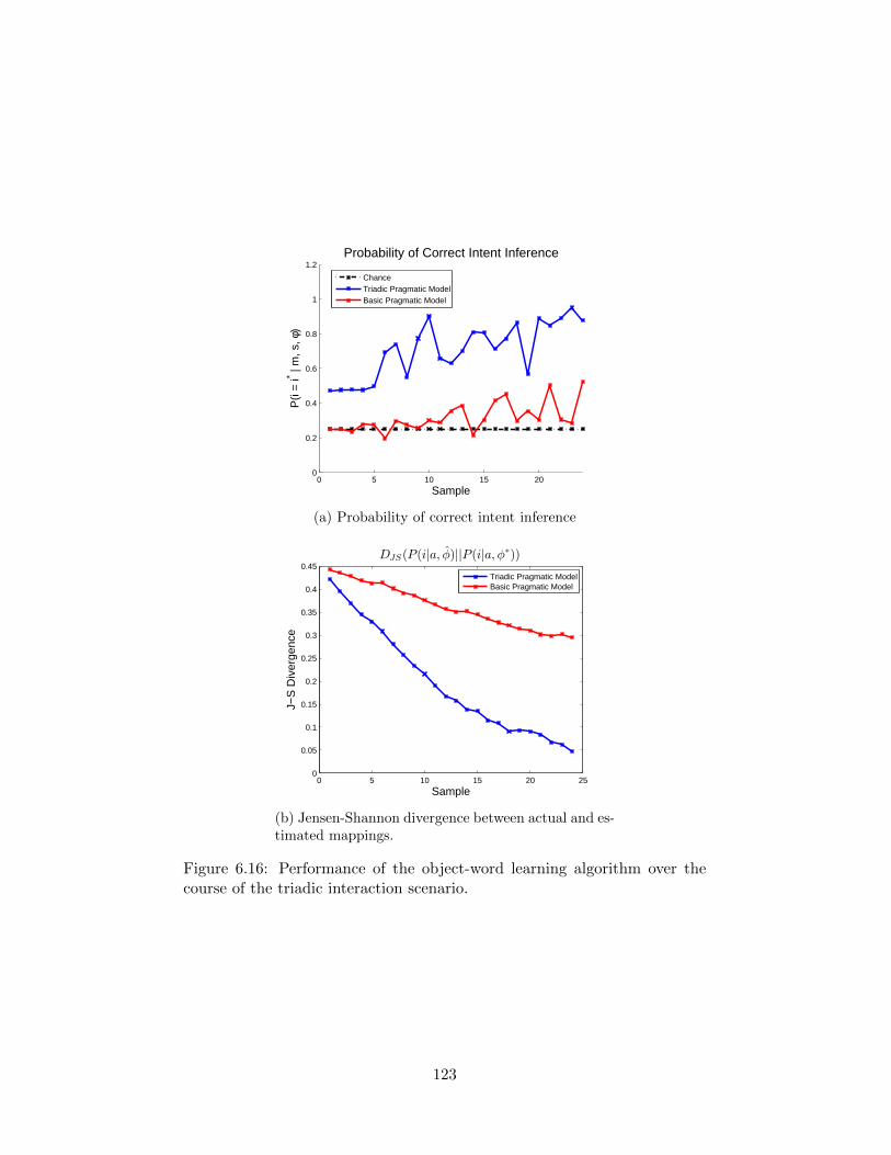
0 5 10 15 200
0.2
0.4
0.6
0.8
1
1.2
P(i
= i* |
m, s
, φ)
Sample
Probability of Correct Intent Inference
ChanceTriadic Pragmatic ModelBasic Pragmatic Model
(a) Probability of correct intent inference
0 5 10 15 20 250
0.05
0.1
0.15
0.2
0.25
0.3
0.35
0.4
0.45
J−S
Div
erge
nce
Sample
DJS(P(i|a, φ)||P(i|a,φ∗))
Triadic Pragmatic ModelBasic Pragmatic Model
(b) Jensen-Shannon divergence between actual and es-timated mappings.
Figure 6.16: Performance of the object-word learning algorithm over thecourse of the triadic interaction scenario.
123
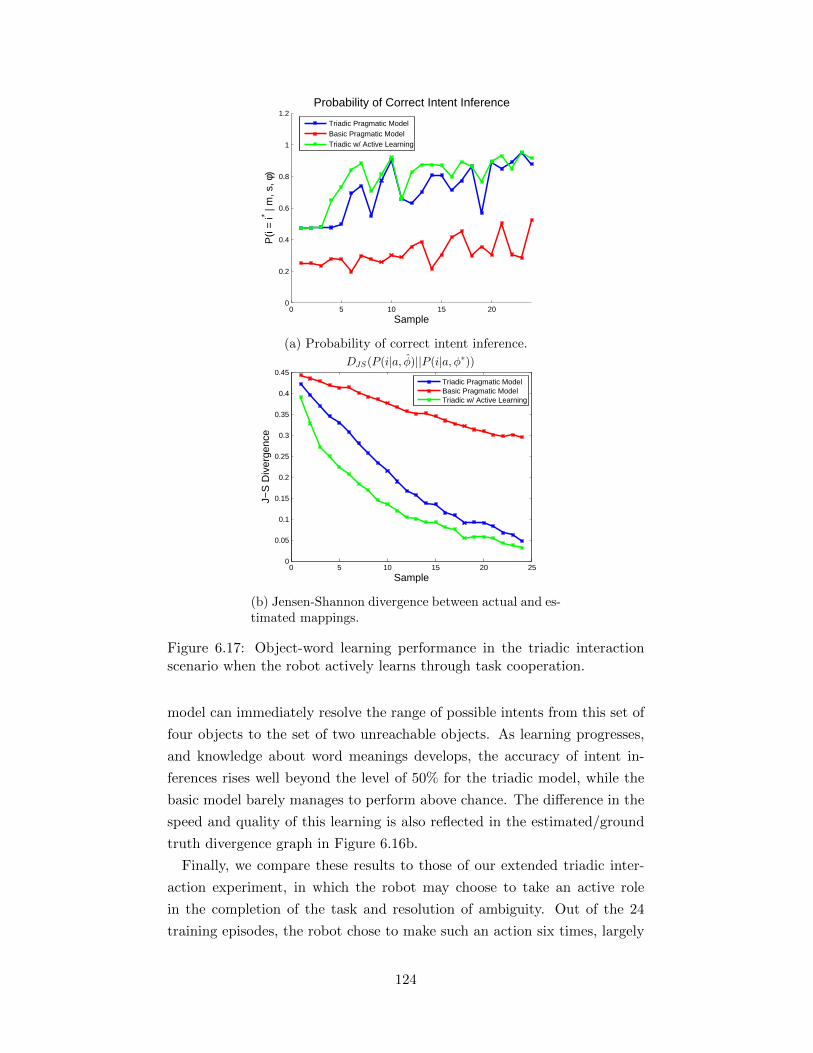
0 5 10 15 200
0.2
0.4
0.6
0.8
1
1.2
P(i
= i* |
m, s
, φ)
Sample
Probability of Correct Intent Inference
Triadic Pragmatic ModelBasic Pragmatic ModelTriadic w/ Active Learning
(a) Probability of correct intent inference.
0 5 10 15 20 250
0.05
0.1
0.15
0.2
0.25
0.3
0.35
0.4
0.45
J−S
Div
erge
nce
Sample
DJS(P(i|a, φ)||P(i|a,φ∗))
Triadic Pragmatic ModelBasic Pragmatic ModelTriadic w/ Active Learning
(b) Jensen-Shannon divergence between actual and es-timated mappings.
Figure 6.17: Object-word learning performance in the triadic interactionscenario when the robot actively learns through task cooperation.
model can immediately resolve the range of possible intents from this set of
four objects to the set of two unreachable objects. As learning progresses,
and knowledge about word meanings develops, the accuracy of intent in-
ferences rises well beyond the level of 50% for the triadic model, while the
basic model barely manages to perform above chance. The difference in the
speed and quality of this learning is also reflected in the estimated/ground
truth divergence graph in Figure 6.16b.
Finally, we compare these results to those of our extended triadic inter-
action experiment, in which the robot may choose to take an active role
in the completion of the task and resolution of ambiguity. Out of the 24
training episodes, the robot chose to make such an action six times, largely
124
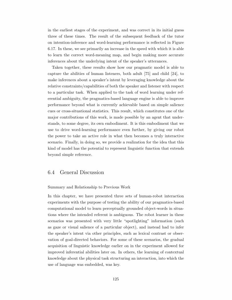
in the earliest stages of the experiment, and was correct in its initial guess
three of these times. The result of the subsequent feedback of the tutor
on intention-inference and word-learning performance is reflected in Figure
6.17. In these, we see primarily an increase in the speed with which it is able
to learn the correct word-meaning map, and begin making more accurate
inferences about the underlying intent of the speaker’s utterances.
Taken together, these results show how our pragmatic model is able to
capture the abilities of human listeners, both adult [75] and child [24], to
make inferences about a speaker’s intent by leveraging knowledge about the
relative constraints/capabilities of both the speaker and listener with respect
to a particular task. When applied to the task of word learning under ref-
erential ambiguity, the pragmatics-based language engine is able to improve
performance beyond what is currently achievable based on simple salience
cues or cross-situational statistics. This result, which constitutes one of the
major contributions of this work, is made possible by an agent that under-
stands, to some degree, its own embodiment. It is this embodiment that we
use to drive word-learning performance even further, by giving our robot
the power to take an active role in what then becomes a truly interactive
scenario. Finally, in doing so, we provide a realization for the idea that this
kind of model has the potential to represent linguistic function that extends
beyond simple reference.
6.4 General Discussion
Summary and Relationship to Previous Work
In this chapter, we have presented three sets of human-robot interaction
experiments with the purpose of testing the ability of our pragmatics-based
computational model to learn perceptually grounded object-words in situa-
tions where the intended referent is ambiguous. The robot learner in these
scenarios was presented with very little “spotlighting” information (such
as gaze or visual salience of a particular object), and instead had to infer
the speaker’s intent via other principles, such as lexical contrast or obser-
vation of goal-directed behaviors. For some of these scenarios, the gradual
acquisition of linguistic knowledge earlier on in the experiment allowed for
improved inferential abilities later on. In others, the learning of contextual
knowledge about the physical task structuring an interaction, into which the
use of language was embedded, was key.
125
The first experiment confirmed the ability of our model and learning al-
gorithms to handle the basic statistical processing capabilities necessary
for learning object-word associations. Additionally, it demonstrated our
model’s capturing of the principle of lexical contrast, one of the fundamen-
tal word-learning abilities present in many previous models [4, 144, 56]. Of
particular relevance are models that focus on the role of incremental learn-
ing [53], or pragmatic, utility-driven reasoning [145]. Unlike these models,
however, our focus has been on the application of this model in an artificial
cognitive system, where the purpose is to ground linguistic symbols in the
multi-modal, situated perceptual representations of our embodied agent.
This situated context aspect becomes even more important in our second
set of experiments, where the robot’s ability to understand linguistic intent
is bound not to a specific perceptual cue (such as gaze), but rather a larger
meaningful task that drives the speaker’s behavior, which itself must be
learned for a particular interaction context. By learning about the physical
task, we can use observations of a speaker’s purposeful action to resolve
referential ambiguity in the word-learning problem in ways not addressed in
previous models. Newer models based in embodied and situated cognitive
agents have begun to use an understanding of action to address other kinds
of linguistic ambiguity, such as determining what perceptual information
is relevant in a form-meaning pair [46]. Here, the physical and linguistic
actions of a task are unified at the level of perception in a way that is much
stronger than our own, while our model captures the connection between
their explicitly goal-directed nature.
It is in the third set of experiments that this deep connection of our
model becomes more fully realized and exploited. Like the previous two
experiments, the robot uses previously acquired knowledge about language
and the task structure. But now, by using an agent’s understanding of the
potential of its own embodiment in the interaction, we are able to use our
pragmatic model to learn word meanings in previously unexplored situa-
tions. Unlike in previous scenarios, there is no way to appeal to gaze or
movement-based salience cues for resolving intent. In this case, the proper
inference of intent is based on a teleological reasoning that involves both
language and action [63], where the robot itself is a means by which the
human speaker is able to achieve his/her goal. And it is through this un-
derstanding that a new kind of functional representation for the meaning of
words emerges. Here a word is not only a tool for influencing the attentional
state of a listener (i.e. reference), but also a way to influence the listener’s
participation in the interaction (i.e. request or command).
126
In our final experiment we begin to explore how we might truly realize
the potential of such a communicative function for the purpose of enhancing
the abilities of our learning agent. For episodes within Experiment III in
which the referent is still ambiguous across a number of objects, we have
our agent make a guess as to the speaker’s intended object, and complete
the task using this object. Essentially, the robot takes control of the system
at the initial state st, for which the observed utterance am is unable to
distinguish between the possible underlying rewards. It then drives it to a
different state s′, with the hope that the new state-action observation (s′, a′),
based on the speaker’s response, will be more useful in disambiguating their
intention. In this situation our pragmatic model functions very similarly to
other active-learning frameworks for estimating an agent’s reward function
[102, 60, 146], some of which also focus on social learning [147]. In relation
to these frameworks, our model is one of the very few that has explored
the use of these ideas in application to the problem of language acquisition.
The capacity for active learning is a product of the explicitly purposeful
representation of language already embedded within our pragmatic model.
We consider this aspect of our model to be a small, but significant step
on the way to constructing artificial cognitive agents for whom language is
something useful.
Limitations
While our implementation of this model in these specific experiments has
demonstrated many new kinds of word-learning capabilities, it also has a
number of limitations, constraints, and areas in need of further development.
Many of these are necessary restrictions on scope and complexity that are
required for feasible study of our model’s core functionality. Others are
limitations of the currently available computational techniques for stochastic
decision and planning in continuous state and action spaces. Two of the most
pressing are the rigidity of our perceptual representations (along with their
processing techniques), and the relatively limited role of embodiment as it
is implemented in our current framework.
One of the first major issues is with the way we represent and perceive the
sensory experience of the robot. In order to develop tractable and practical
applications of our pragmatic framework to the target human-robot word-
learning scenarios, we made some relatively strong assumptions about the
structure of the interaction as it related to the representation of both tasks
and perception. These assumptions included a state space based on visually
127
segmented objects, and their spatial locations. While the IRL algorithm
enables our agent to extract the features of the task that are relevant to the
goal (as shown in Experiment IIb, Figure 6.10a) in an unsupervised manner,
it was fundamentally constrained in the types of goals it could represent.
Relaxing these constraints constitutes a major computational challenge
for our model, as well as most other models of decision, control, and espe-
cially inverse planning. As we scale the size and complexity of our model’s
representations of state, action, and feature spaces, IRL techniques become
intractable due to the necessity of solving the optimal “forward” planning
problem for each possible intent. This is a significant impediment in our
ability to scale the current model beyond the relatively small, simple experi-
mental scenarios we have presented here. However, this is an important and
actively-researched problem, and there have been many promising develop-
ments in scaling IRL techniques to very large representations [148].
In addition to the task component, we were also limited in our represen-
tation of meaning by explicit use of objects as the intentional component
connected to word symbols. This is related to another critical problem with
our current implementation, which is the lack of sophistication in the visual
representation of objects. The color histograms used in the segmentation
and tracking algorithms were the extent of these representations, and the
sole means by which the meanings of words were grounded in the robot’s
perceptual experiences. As a result, these object labels referred to only a
specific visual object within a scene, rather than a broader, perceptually or-
ganized category. More practically, this representation placed a great burden
on the performance of the segmentation and tracking task throughout the
experiment, making these algorithms a significant weak point in the overall
robustness of our computational system. Improving the quality of the visual
processing and representation is one of the most critical problems needing
to be addressed.
Another significant issue is that of the robot’s representation, understand-
ing, and use of its own embodiment within the model. One of the core con-
tributions of this work was to show how such an embodiment and its internal
representation could be exploited to unlock new word learning capabilities.
However, in our current framework, we have given our robot very explicit
knowledge about its embodiment and its potential function. In keeping with
the principles of cognitive development that we have tried our best to adhere
to in the construction of our model, it would be desirable to allow our robot,
at the very least, to learn some of the basic parameters of some representa-
tion through autonomous exploration, as done in a number of other robotic
128
systems (see [149] for a review).
Some of the other limitations that we see in our framework are indicative
of much broader challenges that are topics for long-term research. These in-
clude issues such as autonomous formation of representations for continuous
state, action, and reward spaces, dealing with multi-word utterances, and
co-development of perceptual and conceptual representations, to name but
a few. We will discuss the potential for future exploration of these topics, as
they relate to the pragmatic model we have set forth here, in the concluding
chapter.
129
CHAPTER 7
CONCLUSION
In this thesis, we have shown how techniques for stochastic planning and
control can be applied to a cognitive robotics framework to create a model
for perceptually grounded word learning that captures many of the social
and pragmatic aspects of the same word learning ability in children. This
work was driven by what we believed to be two of the most significant
disparities in the capabilities of robotic systems, relative to their child coun-
terparts. The first was their ability to learn word meanings in cases where
the referent of the word was ambiguous with respect to simple salience or
gaze information. The second was their ability to represent the function or
usefulness of utterances beyond basic reference.
To address these issues, we have constructed a computational framework
that explicitly models the triadic and intentional nature of social interac-
tions, in which words are understood as purposeful actions. The purpose
of these actions is to modulate the listener’s understanding of the speaker’s
goals, such as sharing attention to some object within the environment. We
use a signaling game as the foundation of our model, in which word mean-
ings are represented in terms of how likely they are to produce a certain
interpretation by the listener. Through this representation, we apply tech-
niques for inverse planning to recast the word learning problem from one of
association to one of intentional inference, which we use to derive a basic
algorithm for online word learning.
We further extend this goal-centered representation of language by em-
bedding it within a larger, Markov decision process-based framework for
rational action. This allows us to capture the ways in which children are
able to learn language by understanding their role in the context of a sit-
uated, intentional social interaction. The role may now be for the listener
to recognize some physical task the speaker is performing, or perhaps even
to get the listener to take part in the physical task. We apply techniques
of inverse reinforcement learning to allow our agent to learn goal-centered
representations of these tasks from observations of the speaker. This creates
130
a common ground of knowledge between the speaker and listener that can
then be used to infer the intent of a speaker from physical and/or commu-
nicative actions, which is the critical skill that lies at the heart of a child’s
pragmatic word-learning abilities.
Because the capabilities of our model are only meaningful and useful in
the context of situated, social interactions, they were evaluated within a
set of human-robot interaction experiments, implemented on an iCub hu-
manoid robot. Nearly all elements of our model are, in some way, embedded
in representations of perception and action, some of which we provide a fixed
structure and processing capabilities for. Others, such as representations of
words, are learned through a process of autonomous, incremental construc-
tion of models for sensory experience. In terms of language, we focused on
the learning of words that are grounded in representations of the speech sig-
nal, and corresponding meanings that are grounded in visually segmented
objects.
Through these experiments, we demonstrated the ability of our pragmatic
model to successfully learn these perceptually grounded object-word mean-
ings in scenarios featuring referential ambiguity. These included well-studied
situations requiring skills for basic statistical and contrastive reasoning, for
which the performance of our model matched well with the capabilities seen
in many of the current approaches to the problem. But the significant con-
tribution of our pragmatic framework lies in its ability resolve referential
ambiguity in new kinds of situations, where these more common principles
alone are not enough. These included interactions whose intentional struc-
ture also involved some physical task that is being performed. We showed
how our model could be applied to infer a speaker’s intent based on their
goal-directed physical behaviors by first learning about the intentional reg-
ularities of the task the speaker was performing.
In the final set of experiments, we demonstrated how, by integrating an
understanding of its own embodiment, our robot could reason about its own
potential role in the task in order to resolve ambiguity. We also saw how a
new kind of pragmatic meaning emerges from our model, in which an utter-
ance was used not simply for the purpose of reference, but request. One of
the final contributions of this work was to show how the robot could use its
embodiment to physically realize its requested participation in the interac-
tion, and in doing so actively enhance its own word learning capabilities.
131
7.1 Future Work
As we noted in our general discussion of the model’s application to the set of
human-robot interaction experiments, there are a number of interesting and
challenging ways in which the proposed framework can be developed further.
These include addressing specific technical challenges that are likely to arise
in the extension of our model to new scenarios, as well as more fundamental
questions about what needs to be done to move our linguistic representation
beyond its single word, object-focused implementation.
One of the most exciting and challenging topics for future research is
the development of more advanced representations for the state, action,
and reward components of the model. A critical contribution of this thesis
was in the application of inverse planning techniques to provide our agent
with new and interesting ways to solve the problem of referential ambiguity
in word learning. Currently, most of these techniques scale poorly as the
size of their representation increases, and few have approached the even
more challenging task of working in continuous state and action spaces. In
order for our learner to be able to handle the representational complexity
necessary for modeling more realistic interactions and linguistic usage, we
will need to develop better means for extracting the relevant aspects of
the interaction structure, and more efficient approximations of the optimal
planning problem. Two potential opportunities include integration with
recently developed incremental learning techniques for task representations
[46, 150], and scalable methods for IRL that rely on real-time dynamic
programming approximations [148].
Another significant open issue, which we mentioned early on in this the-
sis, is the lack of representations for meaning that extend beyond reference
to a particular perceptual category. Words with meanings that are largely
social or functional (e.g. “Hello!”, “yes/no”, etc.) have been particularly
neglected. We have attempted, in a small way, to begin addressing this issue
by representing words in terms of their communicative function, which we
used to capture some pragmatic aspects of meaning, such as request. While
the fundamentally triadic nature of our language model lends itself to mean-
ings that are rooted in the mental states of other agents, significant work
needs to be done in order to make these ideas practically implementable,
especially as we move toward multi-word utterances. Given the focus of
our own approach on embodied cognitive systems, one possible candidate
framework to explore is that of Embodied Construction Grammar [151].
132
7.2 Final Remarks
At the outset of this thesis, we set for ourselves the goal of developing a
pragmatics-based model of language acquisition, in order to address some
important issues we perceived to be facing current cognitive systems ap-
proaches. Certainly, these are only one small part of the complete body of
open problems in this area. Likewise, we do not believe our model to be a
complete or accurate computational representation of the complex cognitive
processes that underly the language acquisition capabilities of children, or
even those specific processes that fall under the heading of “pragmatics”.
What we do believe, however, is that the basic pragmatic framework pre-
sented here provides a valuable starting point for the integration of ideas
about the intentional and social nature of communication into future cogni-
tive robotics models of language acquisition.
133
REFERENCES
[1] M. Lungarella, G. Metta, R. Pfeifer, and G. Sandini, “Developmentalrobotics: A survey,” Connection Science, vol. 15, no. 4, pp. 151–190,2003.
[2] D. Vernon, G. Metta, and G. Sandini, “A survey of artificial cognitivesystems: Implications for the autonomous development of mental ca-pabilities in computational agents,” Evolutionary Computation, IEEETransactions on, vol. 11, no. 2, pp. 151–180, 2007.
[3] M. Asada, K. Hosoda, Y. Kuniyoshi, H. Ishiguro, T. Inui,Y. Yoshikawa, M. Ogino, and C. Yoshida, “Cognitive developmentalrobotics: A survey,” Autonomous Mental Development, IEEE Trans-actions on, vol. 1, no. 1, pp. 12–34, May 2009.
[4] C. Yu and D. H. Ballard, “A unified model of early word learning:Integrating statistical and social cues,” Neurocomputing, vol. 70, no.13-15, pp. 2149–2165, 2007.
[5] D. Roy, “Grounded spoken language acquisition: Experiments in wordlearning,” IEEE Transactions on Multimedia, vol. 5, no. 2, pp. 197–209, June 2003.
[6] K. Squire and S. Levinson, “HMM-based semantic learning for a mo-bile robot,” IEEE Transactions on Evolutionary Computation, vol. 11,pp. 199–212, 2007.
[7] N. Iwahashi, “Language acquisition through a human-robot interfaceby combining speech, visual, and behavioral information,” InformationSciences, vol. 156, no. 1-2, pp. 109–121, 2003.
[8] A. Cangelosi and T. Riga, “An embodied model for sensorimo-tor grounding and grounding transfer: Experiments with epigeneticrobots,” Cognitive Science, vol. 30, no. 4, pp. 673–689, 2006.
[9] W. Takano and Y. Nakamura, “Statistically integrated semiotics thatenables mutual inference between linguistic and behavioral symbolsfor humanoid robots,” in Robotics and Automation, 2009. ICRA ’09.IEEE International Conference on, May 2009, pp. 646–652.
134

[10] L. Niehaus and S. E. Levinson, “Online learning and integration ofcomplex action and word lexicons for language grounding,” in De-velopment and Learning and Epigenetic Robotics (ICDL), 2012 IEEEInternational Conference on, Nov. 2012, pp. 1–6.
[11] J. Lipinski, Y. Sandamirskaya, and G. Schoner, “Swing it to the left,swing it to the right: Enacting flexible spatial language using a neu-rodynamic framework,” Cognitive Neurodynamics, vol. 3, no. 4, pp.373–400, 2009.
[12] D. Roy, “Learning visually grounded words and syntax for a scenedescription task,” Computer Speech & Language, vol. 16, no. 3, pp.353–385, 2002.
[13] A. Gopnik, “Three types of early word: The emergence of social words,names and cognitive-relational words in the one-word stage and theirrelation to cognitive development,” First Language, vol. 8, no. 22, pp.49–69, 1988.
[14] L. Bloom, E. Tinker, and C. Margulis, “The words children learn:Evidence against a noun bias in early vocabularies,” Cognitive Devel-opment, vol. 8, no. 4, pp. 431–450, 1993.
[15] B. Schieffelin and E. Ochs, Language Socialization across Cultures.Cambridge University Press, 1987, vol. 3.
[16] E. Newport, H. Gleitman, and L. Gleitman, “Mother, I’d rather do itmyself: Some effects and non-effects of maternal speech style,” Talkingto Children: Language Input and Acquisition, pp. 109–149, 1977.
[17] M. Goddard, K. Durkin, and D. Rutter, “The semantic focus of ma-ternal speech: A comment on Ninio and Bruner (1978),” Journal ofChild Language, vol. 12, no. 1, pp. 209–213, 1985.
[18] E. M. Markman and G. F. Wachtel, “Children’s use of mutual ex-clusivity to constrain the meanings of words,” Cognitive Psychology,vol. 20, no. 2, pp. 121–157, 1988.
[19] G. J. Hollich, K. Hirsh-Pasek, R. M. Golinkoff, R. J. Brand, E. Brown,H. L. Chung, E. Hennon, C. Rocroi, and L. Bloom, “Breaking the lan-guage barrier: An emergentist coalition model for the origins of wordlearning,” Monographs of the Society for Research in Child Develop-ment, pp. i–135, 2000.
[20] M. Tomasello, R. Strosberg, N. Akhtar et al., “Eighteen-month-oldchildren learn words in non-ostensive contexts,” Journal of Child Lan-guage, vol. 23, pp. 157–176, 1996.
[21] N. Akhtar, M. Carpenter, and M. Tomasello, “The role of discoursenovelty in early word learning,” Child Development, vol. 67, no. 2, pp.635–645, 1996.
135
[22] D. Sperber and D. Wilson, Relevance: Communication and Cognition.Cambridge, MA: Harvard University Press, 1986.
[23] M. Tomasello and N. Akhtar, “Two-year-olds use pragmatic cues todifferentiate reference to objects and actions,” Cognitive Development,vol. 10, no. 2, pp. 201–224, 1995.
[24] S. J. Collins, S. A. Graham, and C. G. Chambers, “Preschoolers sensi-tivity to speaker action constraints to infer referential intent,” Journalof Experimental Child Psychology, vol. 112, no. 4, pp. 389–402, 2012.
[25] L. Wittgenstein, Philosophical Investigations. Oxford, UK: Wiley-Blackwell, 2009.
[26] H. Grice, “Meaning,” Philosophical Review, pp. 377–388, 1957.
[27] M. Tomasello, Constructing a Language: A Usage-Based Theory ofLanguage Acquisition. Harvard University Press, 2005.
[28] J. Bruner, Child’s Talk: Learning to Use Language. New York: W.W. Norton & Company, 1985.
[29] A. Turing, “Computing machinery and intelligence,” Mind, vol. 59,pp. 433–460, 1950.
[30] N. Wiener, Cybernetics. New York, NY: J. Wiley, 1948.
[31] N. Wiener, The Human Use of Human Beings: Cybernetics and Soci-ety. Da Capo Press, 1988.
[32] Y. Nagai, H. K., M. A., and A. M., “A constructive model for thedevelopment of joint attention,” Connection Science, vol. 15, pp. 211–229, December 2003.
[33] L. Natale, F. Nori, G. Sandini, and G. Metta, “Learning precise 3dreaching in a humanoid robot,” in Development and Learning, 2007.ICDL 2007. IEEE 6th International Conference on. IEEE, 2007, pp.324–329.
[34] P. Fitzpatrick, G. Metta, L. Natale, S. Rao, and G. Sandini, “Learningabout objects through action-initial steps towards artificial cognition,”in Robotics and Automation, 2003. Proceedings. ICRA’03. IEEE In-ternational Conference on, vol. 3. IEEE, 2003, pp. 3140–3145.
[35] L. Montesano, M. Lopes, A. Bernardino, and J. Santos-Victor, “Learn-ing object affordances: From sensory–motor coordination to imita-tion,” Robotics, IEEE Transactions on, vol. 24, no. 1, pp. 15–26, 2008.
[36] S. Harnad, “The symbol grounding problem,” Physica D, vol. 42, no.1-3, pp. 335–346, 1990.
[37] S. Levinson, Mathematical Models for Speech Technology. New York,NY: John Wiley and Sons Ltd., 2005.
136
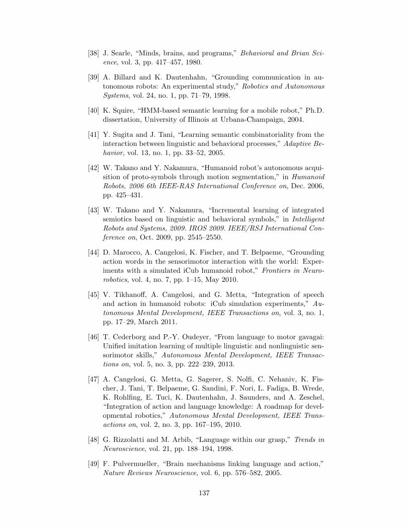
[38] J. Searle, “Minds, brains, and programs,” Behavioral and Brian Sci-ence, vol. 3, pp. 417–457, 1980.
[39] A. Billard and K. Dautenhahn, “Grounding communication in au-tonomous robots: An experimental study,” Robotics and AutonomousSystems, vol. 24, no. 1, pp. 71–79, 1998.
[40] K. Squire, “HMM-based semantic learning for a mobile robot,” Ph.D.dissertation, University of Illinois at Urbana-Champaign, 2004.
[41] Y. Sugita and J. Tani, “Learning semantic combinatoriality from theinteraction between linguistic and behavioral processes,” Adaptive Be-havior, vol. 13, no. 1, pp. 33–52, 2005.
[42] W. Takano and Y. Nakamura, “Humanoid robot’s autonomous acqui-sition of proto-symbols through motion segmentation,” in HumanoidRobots, 2006 6th IEEE-RAS International Conference on, Dec. 2006,pp. 425–431.
[43] W. Takano and Y. Nakamura, “Incremental learning of integratedsemiotics based on linguistic and behavioral symbols,” in IntelligentRobots and Systems, 2009. IROS 2009. IEEE/RSJ International Con-ference on, Oct. 2009, pp. 2545–2550.
[44] D. Marocco, A. Cangelosi, K. Fischer, and T. Belpaeme, “Groundingaction words in the sensorimotor interaction with the world: Exper-iments with a simulated iCub humanoid robot,” Frontiers in Neuro-robotics, vol. 4, no. 7, pp. 1–15, May 2010.
[45] V. Tikhanoff, A. Cangelosi, and G. Metta, “Integration of speechand action in humanoid robots: iCub simulation experiments,” Au-tonomous Mental Development, IEEE Transactions on, vol. 3, no. 1,pp. 17–29, March 2011.
[46] T. Cederborg and P.-Y. Oudeyer, “From language to motor gavagai:Unified imitation learning of multiple linguistic and nonlinguistic sen-sorimotor skills,” Autonomous Mental Development, IEEE Transac-tions on, vol. 5, no. 3, pp. 222–239, 2013.
[47] A. Cangelosi, G. Metta, G. Sagerer, S. Nolfi, C. Nehaniv, K. Fis-cher, J. Tani, T. Belpaeme, G. Sandini, F. Nori, L. Fadiga, B. Wrede,K. Rohlfing, E. Tuci, K. Dautenhahn, J. Saunders, and A. Zeschel,“Integration of action and language knowledge: A roadmap for devel-opmental robotics,” Autonomous Mental Development, IEEE Trans-actions on, vol. 2, no. 3, pp. 167–195, 2010.
[48] G. Rizzolatti and M. Arbib, “Language within our grasp,” Trends inNeuroscience, vol. 21, pp. 188–194, 1998.
[49] F. Pulvermueller, “Brain mechanisms linking language and action,”Nature Reviews Neuroscience, vol. 6, pp. 576–582, 2005.
137
[50] A. Glenberg and M. Kaschak, “Grounding language in action,” Psy-chonomic Bulletin & Review, vol. 9, pp. 558–565, 2002.
[51] L. Steels, “Language games for autonomous robots,” Intelligent Sys-tems, IEEE, vol. 16, no. 5, pp. 16–22, 2001.
[52] F. Forster, C. L. Nehaniv, and J. Saunders, “Robots that say ‘no’,” inAdvances in Artificial Life. Darwin Meets von Neumann. Springer,2011, pp. 158–166.
[53] G. Kachergis, C. Yu, and R. Shiffrin, “An associative model of adap-tive inference for learning word–referent mappings,” Psychonomic Bul-letin & Review, pp. 1–8, 2012.
[54] N. Iwahashi, “Interactive learning of spoken words and their meaningsthrough an audio-visual interface,” IEICE Transactions on Informa-tion and Systems, vol. 91, no. 2, pp. 312–321, 2008.
[55] N. Iwahashi, “Robots that learn language: Developmental approachto human-machine conversations,” Symbol Grounding and Beyond, pp.143–167, 2006.
[56] M. Frank, N. Goodman, and J. Tenenbaum, “Using speakers’ refer-ential intentions to model early cross-situational word learning,” Psy-chological Science, vol. 20, no. 5, pp. 578–585, 2009.
[57] L. Markson, P. Bloom et al., “Evidence against a dedicated system forword learning in children,” Nature, vol. 385, no. 6619, pp. 813–815,1997.
[58] B. McMurray, J. S. Horst, and L. K. Samuelson, “Word learningemerges from the interaction of online referent selection and slow as-sociative learning.” Psychological Review, vol. 119, no. 4, p. 831, 2012.
[59] R. Taguchi, N. Iwahashi, and T. Nitta, “Learning communicativemeanings of utterances by robots,” New Frontiers in Artificial In-telligence, pp. 62–72, 2009.
[60] M. Lopes, T. Cederbourg, and P.-Y. Oudeyer, “Simultaneous acqui-sition of task and feedback models,” in Development and Learning(ICDL), 2011 IEEE International Conference on, vol. 2, 2011, pp.1–7.
[61] J. Grizou, M. Lopes, and P.-Y. Oudeyer, “Robot learning simultane-ously a task and how to interpret human instructions,” in Developmentand Learning and Epigenetic Robotics (ICDL), 2013 IEEE Third JointInternational Conference on. IEEE, 2013, pp. 1–8.
[62] G. Pezzulo, “The interaction engine: A common pragmatic compe-tence across linguistic and nonlinguistic interactions,” AutonomousMental Development, IEEE Transactions on, vol. 4, no. 2, pp. 105–123, 2012.
138
[63] B. Wrede, K. Rohlfing, J. Steil, S. Wrede, P.-Y. Oudeyer, J. Taniet al., “Towards robots with teleological action and language under-standing,” in Humanoids 2012 Workshop on Developmental Robotics:Can Developmental Robotics Yield Human-Like Cognitive Abilities?,2012.
[64] B. Scassellati, “Theory of mind for a humanoid robot,” AutonomousRobots, vol. 12, no. 1, pp. 13–24, 2002.
[65] A. M. Leslie, “ToMM, ToBy, and agency: Core architecture and do-main specificity,” Mapping the Mind: Domain Specificity in Cognitionand Culture, pp. 119–148, 1994.
[66] S. Baron-Cohen, Mindblindness: An Essay on Autism and Theory ofMind. Cambridge, MA: MIT Press, 1997.
[67] Y. Demiris, “Prediction of intent in robotics and multi-agent systems,”Cognitive Processing, vol. 8, no. 3, pp. 151–158, 2007.
[68] S. Augustine, The Confessions, 1876.
[69] R. M. Golinkoff, C. B. Mervis, K. Hirsh-Pasek et al., “Early objectlabels: The case for a developmental lexical principles framework,”Journal of Child Language, vol. 21, pp. 125–155, 1994.
[70] E. Bates, L. Camaioni, and V. Volterra, “The acquisition of performa-tives prior to speech.” Merrill-Palmer Quarterly: Journal of Develop-mental Psychology, 1975.
[71] S. L. James and M. A. Seebach, “The pragmatic function of chil-dren’s questions,” Journal of Speech, Language, and Hearing Research,vol. 25, no. 1, pp. 2–11, 1982.
[72] M. Tomasello and M. Barton, “Learning words in nonostensive con-texts.” Developmental Psychology, vol. 30, no. 5, p. 639, 1994.
[73] N. Akhtar, M. Carpenter, and M. Tomasello, “The role of discoursenovelty in early word learning,” Child Development, vol. 67, no. 2, pp.635–645, 1996.
[74] G. Butterworth and E. Cochran, “Towards a mechanism of joint vi-sual attention in human infancy,” International Journal of BehavioralDevelopment, vol. 3, no. 3, pp. 253–272, 1980.
[75] J. E. Hanna and M. K. Tanenhaus, “Pragmatic effects on referenceresolution in a collaborative task: Evidence from eye movements,”Cognitive Science, vol. 28, no. 1, pp. 105–115, 2004.
[76] A. P. Dempster, N. M. Laird, and D. B. Rubin, “Maximum likelihoodfrom incomplete data via the EM algorithm,” Journal of the RoyalStatistical Society. Series B, pp. 1–38, 1977.
139
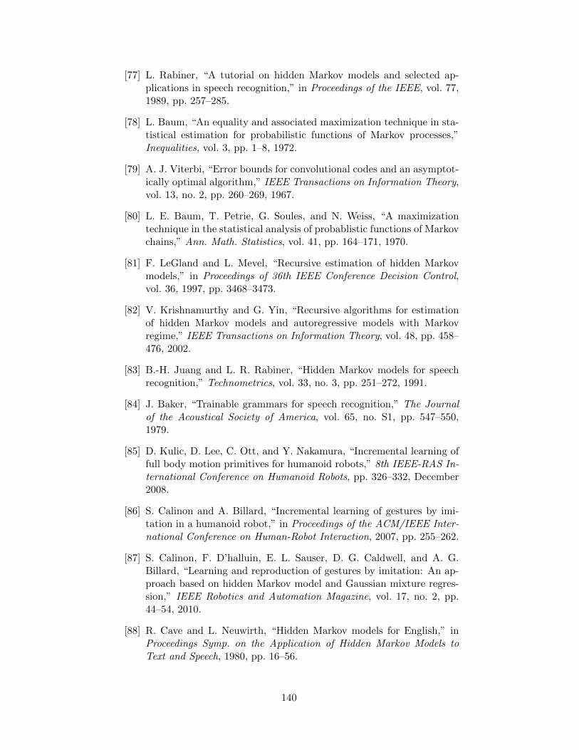
[77] L. Rabiner, “A tutorial on hidden Markov models and selected ap-plications in speech recognition,” in Proceedings of the IEEE, vol. 77,1989, pp. 257–285.
[78] L. Baum, “An equality and associated maximization technique in sta-tistical estimation for probabilistic functions of Markov processes,”Inequalities, vol. 3, pp. 1–8, 1972.
[79] A. J. Viterbi, “Error bounds for convolutional codes and an asymptot-ically optimal algorithm,” IEEE Transactions on Information Theory,vol. 13, no. 2, pp. 260–269, 1967.
[80] L. E. Baum, T. Petrie, G. Soules, and N. Weiss, “A maximizationtechnique in the statistical analysis of probablistic functions of Markovchains,” Ann. Math. Statistics, vol. 41, pp. 164–171, 1970.
[81] F. LeGland and L. Mevel, “Recursive estimation of hidden Markovmodels,” in Proceedings of 36th IEEE Conference Decision Control,vol. 36, 1997, pp. 3468–3473.
[82] V. Krishnamurthy and G. Yin, “Recursive algorithms for estimationof hidden Markov models and autoregressive models with Markovregime,” IEEE Transactions on Information Theory, vol. 48, pp. 458–476, 2002.
[83] B.-H. Juang and L. R. Rabiner, “Hidden Markov models for speechrecognition,” Technometrics, vol. 33, no. 3, pp. 251–272, 1991.
[84] J. Baker, “Trainable grammars for speech recognition,” The Journalof the Acoustical Society of America, vol. 65, no. S1, pp. 547–550,1979.
[85] D. Kulic, D. Lee, C. Ott, and Y. Nakamura, “Incremental learning offull body motion primitives for humanoid robots,” 8th IEEE-RAS In-ternational Conference on Humanoid Robots, pp. 326–332, December2008.
[86] S. Calinon and A. Billard, “Incremental learning of gestures by imi-tation in a humanoid robot,” in Proceedings of the ACM/IEEE Inter-national Conference on Human-Robot Interaction, 2007, pp. 255–262.
[87] S. Calinon, F. D’halluin, E. L. Sauser, D. G. Caldwell, and A. G.Billard, “Learning and reproduction of gestures by imitation: An ap-proach based on hidden Markov model and Gaussian mixture regres-sion,” IEEE Robotics and Automation Magazine, vol. 17, no. 2, pp.44–54, 2010.
[88] R. Cave and L. Neuwirth, “Hidden Markov models for English,” inProceedings Symp. on the Application of Hidden Markov Models toText and Speech, 1980, pp. 16–56.
140
[89] A. Poritz, “Linear predictive hidden Markov models and the speechsignal,” in Proceedings of ICASSP 82. IEEE International Conferenceon Acoustics, Speech and Signal Processing, 1982, pp. 1291–1294.
[90] R. E. Bellman, Dynamic Programming. Princeton, NJ: PrincetonUniversity Press, 1957.
[91] R. Sutton and A. Barto, Reinforcement Learning: An Introduction.Cambridge University Press, 1998.
[92] C. Watkins and P. Dayan, “Q-learning,” Machine Learning, vol. 8, pp.279–292, 1992.
[93] J. Peters and S. Schaal, “Reinforcement learning of motor skills withpolicy gradients,” Neural Networks, vol. 21, no. 4, pp. 682–697, 2008.
[94] T. Mori, Y. Nakamura, M. Sato, and S. Ishii, “Reinforcement learningfor CPG-driven biped robot,” in Proceedings of the National Confer-ence on Artificial Intelligence. AAAI, 2004, pp. 623–630.
[95] E. Carlson and J. Triesch, “A computational model of the emergenceof gaze following,” Progress in Neural Processing, vol. 15, pp. 105–114,2004.
[96] M. Lopes, F. Melo, B. Kenward, and J. Santos-Victor, “A compu-tational model of social-learning mechanisms,” Adaptive Behavior,vol. 17, no. 6, pp. 467–483, 2009.
[97] G. Neu and C. Szepesvari, “Training parsers by inverse reinforcementlearning,” Machine Learning, vol. 77, no. 2-3, pp. 303–337, 2009.
[98] P. Abbeel and A. Y. Ng, “Apprenticeship learning via inverse rein-forcement learning,” in Proceedings of the Twenty-First InternationalConference on Machine Learning. ACM, 2004, p. 1.
[99] N. D. Ratliff, D. Silver, and J. A. Bagnell, “Learning to search: Func-tional gradient techniques for imitation learning,” Autonomous Robots,vol. 27, no. 1, pp. 25–53, 2009.
[100] G. Neu, “Apprenticeship learning using inverse reinforcement learningand gradient methods,” in Proceedings UAI, 2007.
[101] B. Ziebart, A. Maas, J. Bagnell, and A. Dey, “Maximum entropyinverse reinforcement learning,” in Proceedings AAAI, 2008, pp. 1433–1438.
[102] M. Lopes, F. Melo, and L. Montesano, “Active learning for rewardestimation in inverse reinforcement learning,” Machine Learning andKnowledge Discovery in Databases, pp. 31–46, 2009.
[103] D. Ramachandran and E. Amir, “Bayesian inverse reinforcementlearning,” in 20th International Joint Conference on Artificial Intelli-gence, 2007, pp. 2586–2591.
141
[104] B. D. Ziebart, “Modeling purposeful adaptive behavior with the princi-ple of maximum causal entropy,” Ph.D. dissertation, Carnegie MellonUniversity, 2010.
[105] M. Babes, V. Marivate, K. Subramanian, and M. L. Littman, “Ap-prenticeship learning about multiple intentions,” in Proceedings of the28th International Conference on Machine Learning (ICML-11), 2011,pp. 897–904.
[106] R. B. Myerson, Game Theory: Analysis of Conflict. Cambridge, MA:Harvard University Press, 1997.
[107] I.-K. Cho and D. M. Kreps, “Signaling games and stable equilibria,”The Quarterly Journal of Economics, vol. 102, no. 2, pp. 179–221,1987.
[108] P. Parikh, “Communication and strategic inference,” Linguistics andPhilosophy, vol. 14, no. 5, pp. 473–514, 1991.
[109] R. Clark, Meaningful Games: Exploring Language with Game Theory.Cambridge, MA: MIT Press, 2011.
[110] M. Franke, R. Muhlenbernd, and J. Quinley, “Game theoretic prag-matics,” Language Learning, vol. 30, p. 6, 2008.
[111] N. Allott, “Game theory and communication,” Game Theory andPragmatics, pp. 123–151, 2006.
[112] J. Brandts and C. A. Holt, “Adjustment patterns and equilibriumselection in experimental signaling games,” International Journal ofGame Theory, vol. 22, no. 3, pp. 279–302, 1993.
[113] C. M. Anderson and C. F. Camerer, “Experience-weighted attrac-tion learning in sender-receiver signaling games,” Economic Theory,vol. 16, no. 3, pp. 689–718, 2000.
[114] D. Golland, P. Liang, and D. Klein, “A game-theoretic approach togenerating spatial descriptions,” in Proceedings of the 2010 Conferenceon Empirical Methods in Natural Language Processing. Associationfor Computational Linguistics, 2010, pp. 410–419.
[115] E. V. Lieven, “Crosslinguistic and crosscultural aspects of languageaddressed to children,” in Input and Interaction in Language Acqui-sition, C. Gallaway and B. J. Richards, Eds. Cambridge UniversityPress, 1994.
[116] E. V. Clark, “The principle of contrast: A constraint on languageacquisition,” Mechanisms of Language Acquisition, vol. 1, p. 33, 1987.
[117] V. Gallese, L. Fadiga, L. Fogassi, and G. Rizzolatti, “Action recogni-tion in the premotor cortex,” Brain, vol. 119(2), pp. 593–609, 1996.
142
[118] F. Kaplan and V. V. Hafner, “The challenges of joint attention,” In-teraction Studies, vol. 7, no. 2, pp. 135–169, 2006.
[119] C. L. Baker, R. R. Saxe, and J. B. Tenenbaum, “Bayesian theory ofmind: Modeling joint belief-desire attribution,” in Proceedings of theThirty-Second Annual Conference of the Cognitive Science Society,2011, pp. 2469–2474.
[120] T. M. Cover and J. A. Thomas, Elements of Information Theory. NewYork, NY: John Wiley & Sons, 2012.
[121] L. W. Barsalou, “Perceptual symbol systems,” Behavioral and BrainSciences, vol. 22, no. 04, pp. 577–660, 1999.
[122] D. Kulic, W. Takano, and Y. Nakamura, “Online segmentationand clustering from continuous observation of whole body motions,”Robotics, IEEE Transactions on, vol. 25, no. 5, pp. 1158–1166, Oct.2009.
[123] H. Brandl, B. Wrede, F. Joublin, and C. Goerick, “A self-referentialchildlike model to acquire phones, syllables and words from acousticspeech,” in Development and Learning, 2008. ICDL 2008. 7th IEEEInternational Conference on, Aug. 2008, pp. 31–36.
[124] G. Metta, G. Sandini, D. Vernon, L. Natale, and F. Nori, “The iCubhumanoid robot: An open platform for research in embodied cogni-tion,” in PerMIS: Performance Metrics for Intelligent Systems Work-shop, Washington, DC, USA, August 2008, pp. 50–56.
[125] M. S. Malekzadeh, D. Bruno, S. Calinon, T. Nanayakkara, and D. G.Caldwell, “Skills transfer across dissimilar robots by learning context-dependent rewards,” in Intelligent Robots and Systems (IROS), 2013IEEE/RSJ International Conference on. IEEE, 2013, pp. 1746–1751.
[126] P. Fitzpatrick and G. Metta, “Towards long-lived robot genes,”Robotics and Autonomous Systems, vol. 56, pp. 29–45, 2008.
[127] U. Pattacini, F. Nori, L. Natale, G. Metta, and G. Sandini, “An ex-perimental evaluation of a novel minimum-jerk Cartesian controllerfor humanoid robots,” in IEEE/RSJ International Conference on In-telligent Robots and Systems, 2010, pp. 1668–1674.
[128] U. Pattacini, “Modular Cartesian controllers for humanoid robots: De-sign and implementation on the iCub,” Ph.D. dissertation, RBCS,Istituto Italiano di Tecnologia, Genoa, 2010.
[129] J. Canny, “A computational approach to edge detection,” PatternAnalysis and Machine Intelligence, IEEE Transactions on, no. 6, pp.679–698, 1986.
[130] M. J. Swain and D. H. Ballard, “Indexing via color histograms,” inActive Perception and Robot Vision. Springer, 1992, pp. 261–273.
143
[131] G. R. Bradski, “Computer vision face tracking for use in a perceptualuser interface,” 1998.
[132] F. Meyer, “Color image segmentation,” in Image Processing and ItsApplications, International Conference on, 1992, pp. 303–306.
[133] G. Bradski, Dr. Dobb’s Journal of Software Tools, 2000.
[134] H. Hirschmuller, “Stereo processing by semiglobal matching and mu-tual information,” Pattern Analysis and Machine Intelligence, IEEETransactions on, vol. 30, no. 2, pp. 328–341, 2008.
[135] R. Hartley and A. Zisserman, Multiple View Geometry in ComputerVision. Cambridge University Press, 2003.
[136] M. Scaife and J. S. Bruner, “The capacity for joint visual attention inthe infant.” Nature, vol. 253, pp. 265–266, 1975.
[137] B. Lau and J. Triesch, “Learning gaze following in space: A compu-tational model,” in Development and Learning, 2004. ICDL 2004. 3rdIEEE International Conference on, 2004, pp. 57–64.
[138] M. Doniec, G. Sun, and B. Scassellati, “Active learning of joint atten-tion,” in Humanoid Robots, 6th IEEE-RAS International Conferenceon, Dec. 2006, pp. 34–39.
[139] D. Hebb, The Organization of Behavior. New York: Wiley, 1949.
[140] E. Murphy-Chutorian and M. M. Trivedi, “Head pose estimation incomputer vision: A survey,” Pattern Analysis and Machine Intelli-gence, IEEE Transactions on, vol. 31, no. 4, pp. 607–626, 2009.
[141] N. Gourier, D. Hall, and J. L. Crowley, “Estimating face orientationfrom robust detection of salient facial structures,” in FG Net Workshopon Visual Observation of Deictic Gestures, 2004, pp. 1–9.
[142] L. Itti, C. Koch, and E. Niebur, “A model of saliency-based visualattention for rapid scene analysis,” IEEE Transactions Pattern Anal.Mach. Intell., vol. 20, pp. 1254–1259, November 1998.
[143] E. Oja, “Simplified neuron model as a principal component analyzer,”Journal of Mathematical Biology, vol. 15, no. 3, pp. 267–273, 1982.
[144] F. Xu and J. B. Tenenbaum, “Word learning as Bayesian inference.”Psychological Review, vol. 114, no. 2, p. 245, 2007.
[145] N. D. Goodman and A. Stuhlmuller, “Knowledge and implicature:Modeling language understanding as social cognition,” Topics in Cog-nitive Science, vol. 5, no. 1, pp. 173–184, 2013.
[146] A. Baranes and P.-Y. Oudeyer, “Active learning of inverse modelswith intrinsically motivated goal exploration in robots,” Robotics andAutonomous Systems, vol. 61, no. 1, pp. 49–73, 2013.
144
[147] S. Nguyen and P.-Y. Oudeyer, “Active choice of teachers, learningstrategies and goals for a socially guided intrinsic motivation learner,”Paladyn, vol. 3, no. 3, pp. 136–146, 2012.
[148] B. Michini, M. Cutler, and J. P. How, “Scalable reward learning fromdemonstration,” in Robotics and Automation (ICRA), IEEE Interna-tional Conference on, 2013, pp. 303–308.
[149] M. Hoffmann, H. G. Marques, A. Hernandez Arieta, H. Sumioka,M. Lungarella, and R. Pfeifer, “Body schema in robotics: A review,”Autonomous Mental Development, IEEE Transactions on, vol. 2,no. 4, pp. 304–324, 2010.
[150] D. H. Grollman and O. C. Jenkins, “Incremental learning of subtasksfrom unsegmented demonstration,” in Intelligent Robots and Systems(IROS), 2010 IEEE/RSJ International Conference on. IEEE, 2010,pp. 261–266.
[151] N. C.-L. Chang, “Constructing grammar: A computational model ofthe emergence of early constructions,” Ph.D. dissertation, Universityof California, Berkeley, 2009.
145