Embed Size (px)
Citation preview

c© 2014 by Osman Sarood. All rights reserved.
OPTIMIZING PERFORMANCE UNDER THERMAL AND POWER CONSTRAINTSFOR HPC DATA CENTERS
BY
OSMAN SAROOD
DISSERTATION
Submitted in partial fulfillment of the requirementsfor the degree of Doctor of Philosophy in Computer Science
in the Graduate College of theUniversity of Illinois at Urbana-Champaign, 2014
Urbana, Illinois
Doctoral Committee:
Professor Laxmikant V. Kale, ChairProfessor Tarek AbdelzaherProfessor Maria GarzaranDoctor Bronis de Supinski, Lawrence Livermore National Laboratory

Abstract
Energy, power and resilience are the major challenges that the HPC community faces in
moving to larger supercomputers. Data centers worldwide consumed energy equivalent to 235
billion kWh in 2010. A significant portion of that energy and power consumption is devoted
to cooling. This thesis proposes a scheme based on a combination of limiting processor
temperatures using Dynamic Voltage and Frequency Scaling (DVFS) and frequency-aware
load balancing that reduces cooling energy consumption and prevents hot spot formation.
Recent reports have expressed concern that reliability at the exascale level could degrade
to the point where failures become a norm rather than an exception. HPC researchers are
focusing on improving existing fault tolerance protocols to address these concerns. Research
on improving hardware reliability has also been making progress independently. A second
component of this thesis tries to bridge this gap and explore the potential of combining both
software and hardware aspects towards improving reliability of HPC machines. Finally,
the 10MW consumption of present day HPC systems is certainly becoming a bottleneck.
Although energy bills will significantly increase with machine size, power consumption is
a hard constraint that must be addressed. Intel’s Running Average Power Limit (RAPL)
toolkit is a recent feature that enables power capping of CPU and memory subsystems
on modern hardware. The ability to constrain the maximum power consumption of the
subsystems below the vendor-assigned Thermal Design Point (TDP) value allows us to add
more nodes in an overprovisioned system while ensuring that the total power consumption
of the data center does not exceed its power budget. The final component of this thesis
proposes an interpolation scheme that uses an application profile to optimize the number
of nodes and distribution of power between CPU and memory subsystems that minimizes
execution time under a strict power budget. We also present a resource management scheme
including a scheduler that uses CPU power capping, hardware overprovisioning, and job
malleability to improve the throughput of a data center under a strict power budget.
ii

To my parents and wife for their continuous support.
iii

Acknowledgments
Both of you can not do PhD and raise kids. This is what most people told my wife and I
when we started doing PhD and had kids. My super-wife is the sole reason behind my PhD.
How many wives have completed a PhD, took care of a husband and raised 2 kids all at
the same time? I remember her taking care of our new born and our 2 year old daughter
immediately after her C-section while I had to go for work. I would never be able to repay
her for that!
It was my parents determination that brought me to the US to pursue higher studies. I
still remember their kind words that made me believe in myself. My father sacrificed his
career in order to spare time for me, while my mother would spend her nights praying to
Allah (God) for my success. I still remember her standing with me on my PhD defense and
saying: 6 saal sey iss din ka intezar kiya (I have waited 6 years for this day). My grand
father, Prof. Anjum Roomani, also played a very vital role in my studies and upbringing.
May he rest in peace. I would also thank my brother, Omer Sarood, for supporting me to
go for graduate studies. I also owe a lot to my sister, Amna Sarood, who has been praying
for both my wife and I throughout our PhD. I like to thank my friends Musa, Rana, and
Ghufran for taking care of my parents while I was in the US.
I thank Prof. Laxmikant Kale for being a generous and helping advisor. He taught me
so many things from paper writing to exploring groundbreaking ideas. His emphasis on
experimental work is something that greatly contributed to the quality of my work. Besides
my advisor, I thank Prof. Bronis de Supinski and Prof. Maria Garzaran for serving on my
doctoral committee and providing valuable perspectives on improving the dissertation.
I would like to thank my internship supervisor Barry Rountree, who played a key role
towards the end of my thesis. Barry introduced me to the wonderful world of mathematical
modeling and linear programming which facilitated the latter part of my research.
I would sincerely like to thank Prof. Tarek Abdelzaher for allowing us to use the Power
iv

and Energy clusters. Without getting access to these clusters this thesis would not have
been possible.
I am privileged to have worked with some of the most competent people in the world, i.e.
my lab mates. I spent hours talking to most of them and learnt a lot from them. Esteban is
a very good team player and I loved discussing my work with him. Some of our discussions
led to very good projects. Akhil is a very smart person and would point out problems that
most people would fail to identify. I owe a lot of credit to Phil for helping me out with my
experimental work. Jonathan and Nikhil are both very competent and wonderful people to
interact with. I enjoyed co-authoring a lot of papers with Abhishek due to his reliability.
Lukasz, Dave, Abhinav, Eric, Isaac, and Pritish helped me during my initial days at the
PPL. Harshitha and Ram were gentle colleagues with whom I had a lot of discussions about
raising kids. I will miss discussing my power related work with Ehsan. The new generation
of PPLers, Mike, Ronak, Bilge remind me of my early days. I would like to thank JoAnne
for writing all those numerous HR related letters for me.
During my stay at Urbana-Champaign I was blessed to have the company of some amazing
people. This town won’t have been so much fun for me without Azeem bhai and Qazi bhai.
I would miss all those night-long discussions we had. Syed Usman Ali is the most lively
person I have ever met. I would miss playing cricket in the South Quad, especially alongside
Ahmad Qadir.
Last but not least, I would like to thank everyone I met at Urbana during my stay. I may
not remember their names but they made a difference in one of the most exciting adventures
of my life.
v

Grants
This work was partially supported by the following sources:
• HPC Colony II. This project is funded by the US Department of Energy under grant
DOE DE-SC0001845. The Principal Investigator of this project is Terry Jones.
• Simplifying Parallel Programming for CSE Applications using a Multi-
Paradigm Approach. This project is funded by the National Science Foundation
(NSF) under grant NSF ITR-HECURA-0833188. It is a collaborative work between
Prof. Laxmikant Kale, Prof. David Padua and Prof. Vikram Adve.
• Power/Energy Cluster. This project is funded by the National Science Foundation
(NSF) under grant NSF CNS 09- 58314. The Principal Investigator of this project is
Prof. Tarek Abdelzaher.
vi

Table of Contents
List of Figures . . . . . . . . . . . . . . . . . . . . . . . . . . . . . . . . . . . . . . . ix
List of Tables . . . . . . . . . . . . . . . . . . . . . . . . . . . . . . . . . . . . . . . . xii
List of Algorithms . . . . . . . . . . . . . . . . . . . . . . . . . . . . . . . . . . . . . xiii
CHAPTER 1 Introduction . . . . . . . . . . . . . . . . . . . . . . . . . . . . . . . . 11.1 Thesis Organization . . . . . . . . . . . . . . . . . . . . . . . . . . . . . . . . 3
CHAPTER 2 Thermal Restraint Using Migratable Objects . . . . . . . . . . . . . . 52.1 Related Work . . . . . . . . . . . . . . . . . . . . . . . . . . . . . . . . . . . 62.2 Limiting Temperatures . . . . . . . . . . . . . . . . . . . . . . . . . . . . . . 82.3 Charm++ and Load Balancing . . . . . . . . . . . . . . . . . . . . . . . . . 102.4 ‘Cool’ Load Balancer . . . . . . . . . . . . . . . . . . . . . . . . . . . . . . . 122.5 Experimental Setup . . . . . . . . . . . . . . . . . . . . . . . . . . . . . . . . 152.6 Constraining Core Temperatures and Timing Penalty . . . . . . . . . . . . . 172.7 Energy Savings . . . . . . . . . . . . . . . . . . . . . . . . . . . . . . . . . . 232.8 Tradeoff in Execution Time and Energy Consumption . . . . . . . . . . . . . 32
CHAPTER 3 Thermal Restraint and Reliability . . . . . . . . . . . . . . . . . . . . 353.1 Related Work . . . . . . . . . . . . . . . . . . . . . . . . . . . . . . . . . . . 363.2 Implications of Temperature Control . . . . . . . . . . . . . . . . . . . . . . 373.3 Approach . . . . . . . . . . . . . . . . . . . . . . . . . . . . . . . . . . . . . 423.4 Experiments . . . . . . . . . . . . . . . . . . . . . . . . . . . . . . . . . . . . 473.5 Projections . . . . . . . . . . . . . . . . . . . . . . . . . . . . . . . . . . . . 55
CHAPTER 4 Optimizing Performance Under a Power Budget . . . . . . . . . . . . 604.1 Related Work . . . . . . . . . . . . . . . . . . . . . . . . . . . . . . . . . . . 624.2 Approach . . . . . . . . . . . . . . . . . . . . . . . . . . . . . . . . . . . . . 624.3 Setup . . . . . . . . . . . . . . . . . . . . . . . . . . . . . . . . . . . . . . . . 654.4 Case Study: Lulesh . . . . . . . . . . . . . . . . . . . . . . . . . . . . . . . . 654.5 Results . . . . . . . . . . . . . . . . . . . . . . . . . . . . . . . . . . . . . . . 69
vii

CHAPTER 5 Job Scheduling Under a Power Budget . . . . . . . . . . . . . . . . . 795.1 Related work . . . . . . . . . . . . . . . . . . . . . . . . . . . . . . . . . . . 805.2 Data Center and Job Capabilities . . . . . . . . . . . . . . . . . . . . . . . . 815.3 The Resource Manager . . . . . . . . . . . . . . . . . . . . . . . . . . . . . . 825.4 Strong Scaling Power Aware Model . . . . . . . . . . . . . . . . . . . . . . . 875.5 Experimental Results . . . . . . . . . . . . . . . . . . . . . . . . . . . . . . . 905.6 Large Scale Projections . . . . . . . . . . . . . . . . . . . . . . . . . . . . . . 97
CHAPTER 6 Concluding Remarks . . . . . . . . . . . . . . . . . . . . . . . . . . . 1076.1 Thermal Restraint . . . . . . . . . . . . . . . . . . . . . . . . . . . . . . . . 1076.2 Power Constraint . . . . . . . . . . . . . . . . . . . . . . . . . . . . . . . . . 109
APPENDIX A Machine Descriptions . . . . . . . . . . . . . . . . . . . . . . . . . . 112
APPENDIX B Benchmark Descriptions . . . . . . . . . . . . . . . . . . . . . . . . . 114
REFERENCES . . . . . . . . . . . . . . . . . . . . . . . . . . . . . . . . . . . . . . . 117
viii
List of Figures
1.1 Mean Time Between Failures (MTBF) for different numbers of socketsusing different MTBF per socket. . . . . . . . . . . . . . . . . . . . . . . . . 2
1.2 Power consumption and theoretical peak performance for supercomputersfrom the Top500 (blue circles). The proposed Exascale machine under apower budget of 20MW (red square). . . . . . . . . . . . . . . . . . . . . . . 3
2.1 Average core temperatures and maximum difference of any core from theaverage for Wave2D . . . . . . . . . . . . . . . . . . . . . . . . . . . . . . . 9
2.2 Execution time and energy consumption for Wave2D running at differentCRAC set-points using DVFS . . . . . . . . . . . . . . . . . . . . . . . . . . 10
2.3 Our DVFS and load balancing scheme successfully keeps all processorswithin the target temperature range of 47◦–49◦ C, with a CRAC set-pointof 24.4◦ C. . . . . . . . . . . . . . . . . . . . . . . . . . . . . . . . . . . . . . 18
2.4 Execution timing penalty with and without Temperature Aware LoadBalancing . . . . . . . . . . . . . . . . . . . . . . . . . . . . . . . . . . . . . 19
2.5 Execution timelines before and after Temperature Aware Load Balancingfor Wave2D . . . . . . . . . . . . . . . . . . . . . . . . . . . . . . . . . . . . 20
2.6 Minimum core frequencies produced by DVFS for different applications at24.4◦ C . . . . . . . . . . . . . . . . . . . . . . . . . . . . . . . . . . . . . . . 21
2.7 Average core frequencies produced by DVFS for different applications at24.4◦ C . . . . . . . . . . . . . . . . . . . . . . . . . . . . . . . . . . . . . . . 21
2.8 Average frequency of processors for Jacobi2D using TempLDB . . . . . . . . 222.9 Utilization of processors for Jacobi2D using TempLDB . . . . . . . . . . . . 222.10 Frequency sensitivity of the various applications . . . . . . . . . . . . . . . . 232.11 Machine and cooling power consumption for no-DVFS runs at a 12.2 ◦C
set-point and various TempLDB runs . . . . . . . . . . . . . . . . . . . . . . 252.12 Savings in cooling energy consumption with and without Temperature
Aware Load Balancing (higher is better) . . . . . . . . . . . . . . . . . . . . 272.13 Change in machine energy consumption with and without Temperature
Aware Load Balancing (values less than 1 represent savings) . . . . . . . . . 282.14 Normalized machine energy consumption for different frequencies using
128 cores . . . . . . . . . . . . . . . . . . . . . . . . . . . . . . . . . . . . . . 30
ix

2.15 The time Wave2D spent in different frequency levels . . . . . . . . . . . . . 302.16 Total power draw for the cluster using TempLDB at CRAC set-point
of 24.4 ◦C . . . . . . . . . . . . . . . . . . . . . . . . . . . . . . . . . . . . . 312.17 Power consumption of two applications as their DVFS settings stabilize to
a steady state . . . . . . . . . . . . . . . . . . . . . . . . . . . . . . . . . . . 312.18 Timing penalty and energy savings of TempLDB and RefineLDB com-
pared to naive DVFS . . . . . . . . . . . . . . . . . . . . . . . . . . . . . . . 322.19 Normalized time against normalized total energy for a representative sub-
set of applications . . . . . . . . . . . . . . . . . . . . . . . . . . . . . . . . . 33
3.1 Histogram of max temperature for each node of the cluster using Wave2D . 383.2 Effect of cooling down processors on MTBF of the system . . . . . . . . . . 393.3 Dynamic power management and resilience framework. . . . . . . . . . . . . 473.4 Reduction in execution time for different temperature thresholds . . . . . . . 503.5 Execution time penalty for DVFS . . . . . . . . . . . . . . . . . . . . . . . . 533.6 Gains/cost of increasing reliability for different temperature thresholds . . . 543.7 Reduction in machine energy consumption for all applications . . . . . . . . 563.8 Execution time reduction for all applications at large scale . . . . . . . . . . 573.9 Projected efficiency for Wave2D . . . . . . . . . . . . . . . . . . . . . . . . . 583.10 Reduction in execution time for different memory sizes of an
exascale machine . . . . . . . . . . . . . . . . . . . . . . . . . . . . . . . . . 59
4.1 Average time per step of Lulesh for configurations selected in Step 1 . . . . . 664.2 Average time per step of Lulesh after interpolation (Step 2) . . . . . . . . . 684.3 Speedups obtained using CPU and memory power capping in an over-
provisioned system . . . . . . . . . . . . . . . . . . . . . . . . . . . . . . . . 694.4 Observed speedups using different number of profile configurations (points)
as input to our interpolation scheme . . . . . . . . . . . . . . . . . . . . . . 724.5 Optimized CPU and memory power caps under different power budgets
compared to the maximum CPU and memory power drawn in the baselineexperiments . . . . . . . . . . . . . . . . . . . . . . . . . . . . . . . . . . . . 73
4.6 Optimal number of nodes under different total power budgets . . . . . . . . 744.7 Speedups over the case of pc = 25W for different number of nodes (n) . . . . 744.8 Measured CPU and memory power for two different configurations with
significantly different power allocations but similar execution time . . . . . . 764.9 Speedups for power capping both CPU and memory (C&M) compared to
CPU (C) only . . . . . . . . . . . . . . . . . . . . . . . . . . . . . . . . . . . 774.10 Estimated speedups for different base powers in case of P=800W . . . . . . 77
5.1 A high level overview of PARM . . . . . . . . . . . . . . . . . . . . . . . . . 835.2 Integer Linear Program formulation of PARM scheduler . . . . . . . . . . . . 855.3 Model estimates (line) and actual measured (circles) execution times for
all applications as a function of CPU power (a-e). Modeled power awarespeedups for all applications (f). . . . . . . . . . . . . . . . . . . . . . . . . . 92
x

5.4 Modeled (lines) and observed (markers) power aware speedups for fourapplications . . . . . . . . . . . . . . . . . . . . . . . . . . . . . . . . . . . . 93
5.5 (a) Average completion times, and (b) average response times for SetLand SetH with SLURM and noSE, wSE versions of PARM. (c) Averagenumber of nodes and average CPU power in the wSE and noSE versionsof PARM. . . . . . . . . . . . . . . . . . . . . . . . . . . . . . . . . . . . . . 96
5.6 Average completion times of baseline, noSE and wSE. Job arrival times inall the sets (Set1, Set2, Set3) were scaled down by factor γ to get diversityin job arrival rate . . . . . . . . . . . . . . . . . . . . . . . . . . . . . . . . . 100
5.7 Reduction in job arrival times while maintaining the same QoS as thebaseline scheduler . . . . . . . . . . . . . . . . . . . . . . . . . . . . . . . . . 103
5.8 Average completion times for Set 1 for different values of (α) . . . . . . . . . 1045.9 Maximum (worst) completion times for Set 1 for different values of (α) . . . 1045.10 CDF for completion times for baseline and wiSE for different α using SET1 . 1055.11 Effect of increasing the number of power levels (|Pj|) on the average com-
pletion time of Set 1 (γ = 0.5). . . . . . . . . . . . . . . . . . . . . . . . . . 1065.12 Effect of increasing the number of power levels (|Pj|) on the maximum
completion time of Set 1 (γ = 0.5). . . . . . . . . . . . . . . . . . . . . . . . 106
xi
List of Tables
2.1 Description for variables used in Algorithm 1 . . . . . . . . . . . . . . . . . . 132.2 Performance counters for Charm++ applications on one core . . . . . . . . . 21
3.1 Parameters of the performance model . . . . . . . . . . . . . . . . . . . . . . 413.2 Description for variables used in Algorithm 2 and Algorithm 3 . . . . . . . . 433.3 Application parameters for NC case . . . . . . . . . . . . . . . . . . . . . . 493.4 MTBF (sec) for different temperature thresholds (42◦ C - 54◦ C) . . . . . . . 51
4.1 Terminology . . . . . . . . . . . . . . . . . . . . . . . . . . . . . . . . . . . . 63
5.1 Integer Linear Program Terminology . . . . . . . . . . . . . . . . . . . . . . 845.2 Obtained model parameters . . . . . . . . . . . . . . . . . . . . . . . . . . . 945.3 Comparison of the baseline, wSE and noSE scheduling policies for different
data sets. . . . . . . . . . . . . . . . . . . . . . . . . . . . . . . . . . . . . . 1015.4 Comparison of wSE with the baseline scheduler running on an overprovi-
sioned system (at different CPU power caps) using Set 2 (γ = 0.5) . . . . . . 102
A.1 Summary of features of clusters used in this thesis . . . . . . . . . . . . . . . 112
xii

List of Algorithms
1 Temperature Aware Refinement Load Balancing . . . . . . . . . . . . . . . . 14
2 Temperature Control . . . . . . . . . . . . . . . . . . . . . . . . . . . . . . . 45
3 Communication Aware Load Balancing . . . . . . . . . . . . . . . . . . . . . 46
xiii
CHAPTER 1Introduction
Computational scientists are among the leading users of high performance computing (HPC).
These scientists usually run codes that simulate physical processes. Such simulation codes
have an everlasting demand for computational power. In order to satisfy the demands
for running these computational models, the HPC community will need to keep advancing
their quest for larger machines. Soaring energy consumption, accompanied by declining
reliability, together loom as the biggest hurdles for the next generation of supercomputers.
As we approach the exascale era, both hardware and software designers will need to account
for power, energy, and reliability of the machine while optimizing performance.
The combined energy consumption for data centers worldwide totaled 235 billion kWh in
2010 [1]. Most HPC researchers have been primarily focussing on energy minimization in
the past decade [2,3]. The majority of this work is concentrated on reducing machine energy
consumption. In this dissertation, we first attack the ‘other’ side of the problem i.e., cooling
energy consumption, which can account for up to 50% of the total energy consumption of
a data center [4–7]. Chip manufacturers have ceased to increase processor frequency and
have resorted to adding more cores on a chip to keep up with the ever increasing demand
for faster computers. This stagnation in processor frequency has been caused by a sharp
increase in the heat density of chip. Earlier studies show a connection between the operating
temperature of a processor and its reliability [8–10]. These studies mention the existence of
an exponential relationship between a processor’s temperature and its Mean Time Between
Failures (MTBF). Most HPC research focused on energy optimization and machine reliability
does not consider the impact of processor temperature. Although thermal considerations
have not been a primary concern for recent supercomputers, it can significantly improve
MTBF and hence, performance of future supercomputers. An exascale machine is predicted
to have more than 200,000 sockets [11]. Recent studies also show that supercomputers can
1

200K 300K 400K 500K8
26
52
131
262
Number of Sockets
Machin
e M
TB
F (
min
s)
100y50y20y10y
Figure 1.1: Mean Time Between Failures (MTBF) for different numbers of sockets usingdifferent MTBF per socket.
have a per socket MTBF as low as 5 years [12]. The implications of such large numbers
of sockets coupled with the existing MTBF values per socket are depicted in Figure 1.1.
This figure shows the MTBF of large supercomputers for different numbers of sockets and
different MTBF per socket. Figure 1.1 shows that with a per socket MTBF of 5 years, a
200K socket machine is likely to fault every 26 mins. Such a high fault rate could have a
dramatic effect on machine utilization. On the other hand, a per socket MTBF of 100 years
can improve the machine reliability and increase the machine MTBF to 262 mins for a 200K
socket machine. This thesis makes an attempt at improving the per socket MTBF of a large
machine by using Dynamic Voltage and Frequency Scaling (DVFS) in conjunction with an
adaptive runtime system.
Although energy minimization and thermal control are major challenges, in order to reach
exascale computing within the 20MW power envelope proposed by the DOE, data cen-
ters would have to significantly improve their performance per watt. Figure 1.2 shows the
power consumption and the theoretical peak performance of all the supercomputers from
the Top500 [13] for which power consumption data is available (blue circles). It also plots
the power consumption bound (20MW) set by the DOE for the exascale machine (red box).
Given the trend of current supercomputers, it is unlikely that the HPC community will
achieve exascale computing within the 20MW power budget. Looking at the data from
Figure 1.2, 100MW seems to be a more realistic target to achieve an exaflop. Although
2

101
102
103
104
105
1014
1015
1016
1017
1018
1019
Theore
tical peak p
erf
orm
ance (
FLO
Ps)
Power consumption (kW)
Figure 1.2: Power consumption and theoretical peak performance for supercomputers fromthe Top500 (blue circles). The proposed Exascale machine under a power budget of 20MW(red square).
hardware advances will be needed to build an exascale machine, efficient runtime techniques
are necessary to make the best use of what the hardware will provide.
1.1 Thesis Organization
This thesis is organized in three major parts. Part one contains Chapter 2 and Chapter 3.
This part demonstrates techniques for controlling core temperature and their impact on
performance and reliability. Chapter 2 describes how Dynamic Voltage and Frequency Scal-
ing (DVFS) can restrain processor temperatures and our scheme that uses object migration
to minimize the timing penalty associated with DVFS. Chapter 2 further presents the ex-
perimental results for restraining processor temperatures using different applications, and
demonstrates the reduction in timing penalty as well as energy consumption. It includes
a comprehensive discussion about application reaction to thermal restraint. Chapter 3 in-
troduces a novel technique that combines fault tolerance with thermal restraint to improve
system reliability. It demonstrates how restraining core temperatures can eventually ben-
efit application performance as a result of improved machine reliability. It also presents
the estimated benefits in machine reliability and application performance of using temper-
3

ature restraint for massively parallel machines running different types of applications. We
thank Esteban Meneses for his interest in the research on improving reliability using ther-
mal restraint (Chapter 3). We had a lot of discussions which helped improve the quality
of our work. In particular, Esteban’s incisive comments and his mathematical modeling
background helped us a great deal.
Part two of the thesis tackles the imminent problem of data center operation under a
strict power budget. It contains Chapters 4 and Chapters 5. Operating under a power
constraint is a challenging problem as it poses a constraint rather than a restraint which is
a less stricter limiting condition. While restraining, we try to apply a limit whereas in case
of a constraint that limit is strictly enforced. In this part, we use Intel’s Running Average
Power Library (RAPL) to cap processor and memory power for overprovisioned systems [14]
to improve application performance. Chapter 4 uses RAPL to improve application perfor-
mance for a single application executing in an overprovisioned system. Chapter 5 proposes
a resource management strategy that maximizes job throughput by intelligently scheduling
applications with different resource configurations. This chapter also proposes a detailed
strong scaling power aware model that can estimate the execution time of an application
based on its characteristics for any resource configuration. We thank Akhil Langer for his
interest in the research on optimization under strict power budget (Chapter 4 and 5). We
had numerous productive discussions during which we gave direction to this work. In partic-
ular, his insightful comments, his linear programming background, his work on the SLURM
simulator, and clear presentation of the ideas (including writing of the papers) helped us a
great deal.
Chapter 6 contains the last part of the thesis which summarizes the contributions of this
thesis and possible directions for future work. We outline multiple directions in which we
plan to extend our thesis work. The first idea relates to improving machine reliability by
taking into account the effects of thermal throttling. The second idea explores the possibility
of operating a data center under strict power and thermal constraints.
4

CHAPTER 2Thermal Restraint Using Migratable Objects
Energy consumption has emerged as a significant issue in modern high-performance com-
puting systems. Some of the largest supercomputers draw more than 10 megawatts, leading
to millions of dollars per year in energy bills. What is perhaps less well known is the fact
that 40% to 50% of the energy consumed by a data center is spent in cooling [4], [5], [6], to
keep the computer room running at a lower temperature. How can we reduce this cooling
energy?
Increasing the thermostat setting on the computer room air-conditioner (CRAC) reduces
the cooling power. But the increase in the thermostat will also increase the ambient tem-
perature in the computer room. The reason the ambient temperature is kept cool is to
keep processor cores from overheating. If they run at a high temperature for a long time,
the processor cores may be damaged. Additionally, cores consume more energy per unit of
work when run at higher temperatures [15]. Further, due to variations in the air flow in
the computer room, some chips may not be cooled as effectively as the rest. Semiconduc-
tor process variation will also likely contribute to variability in heating, especially in future
processor chips. So, to handle such ‘hot spots’, the ambient air temperature is kept at a low
temperature to ensure that no individual chip overheats.
Modern microprocessors contain on-chip temperature sensors that can be accessed by
software with minimal overhead. Further, they also provide means to change the frequency
and voltage at which the chip runs, known as dynamic voltage and frequency scaling, or
DVFS. Running processor cores at a lower frequency (and correspondingly lower voltage)
reduces the thermal energy that they dissipate, leading to a cool-down.
This suggests a method for keeping processors cool while increasing the CRAC set-point
(i.e. the thermostat setting). A component of the application software can periodically
check the temperature of the chip. When it exceeds a pre-set threshold, the software can
5

reduce the frequency and voltage of that particular chip. If the temperature is lower than a
threshold, the software can correspondingly increase the frequency.
This technique will ensure that no processors overheat. However, in HPC computations,
and specifically in tightly-coupled science and engineering simulations, DVFS creates a new
problem. Generally, computations on one processor are dependent on the data produced by
the other processors. As a result, if one processor slows down to half its original speed, the
entire computation can slow substantially, in spite of the fact that the remaining processors
are running at full speed. Thus, such an approach will reduce the cooling power, but increase
the execution time of the application. Running the cooling system for a longer time can also
increase the cooling energy.
We aim to reduce cooling power without substantially increasing execution time, and thus
reduce cooling energy. We first describe the temperature sensor and frequency control mech-
anisms, and quantify their impact on execution time mentioned above (Section 2.2). Our
solution leverages the adaptive runtime system underlying the Charm++ parallel program-
ming system (Section 2.3). In order to minimize total system energy consumption, we study
an approach of limiting CPU temperatures via DVFS and mitigating the resultant timing
penalties with a load balancing strategy that is conscious of these effects (Section 2.4). We
show the impact of this combined technique on application performance (Section 2.6) and
total energy consumption (Section 2.7).
2.1 Related Work
Cooling energy optimization and hot spot avoidance have been addressed extensively in the
literature of non-HPC data centers [16–19], which shows the importance of the topic. As
an example, job placement and server shut down have shown savings of up to 33% in cool-
ing costs [16]. Many of these techniques rely on placing jobs that are expected to generate
more heat in the cooler areas of the data center. Such job placement schemes can not be
directly applied to HPC applications because different nodes are running parts of the same
application with similar power consumption. As an example, Rajan et al [20] use system
throttling for temperature-aware scheduling in the context of operating systems. Given their
assumptions, they show that keeping temperature constant is beneficial with their theoretical
models. However, their assumption of non-migratability of tasks is not true in HPC applica-
tions, especially with an adaptive runtime system. Le et al. [21] constrain core temperatures
by turning the machines on and off and consequently reduce total energy consumption by
18%. However, most of these techniques, cannot be applied to HPC applications as they are
6

not practical for tightly-coupled applications.
Minimizing energy consumption has also been an important topic for HPC researchers.
However, most of the work has focused on machine energy consumption rather than cool-
ing energy. Freeh et al. [2] show machine energy savings of up to 15% by exploiting the
communication slack present in the computational graph of a parallel application. Lim et
al [22] demonstrate a median energy savings of 15% by dynamically adjusting the CPU
frequency/voltage pair during the communication phases in MPI applications. Springer et
al. [3] generate a frequency schedule for a DVFS-enabled cluster that runs the target appli-
cation. This schedule tries to minimize the execution time while staying within the power
constraints. The major difference of our approach to the ones mentioned is that our DVFS
decisions are based on saving cooling energy consumption by constraining core temperatures.
The total energy consumption savings that we report represent both machine and cooling
energy consumption.
Huang and Feng describe a kernel-level DVFS governor that tries to determine the power-
optimal frequency for the expected workload over a short time interval that reduces machine
energy consumption up to 11% [23]. Hanson et al. [24] devise a runtime system named PET
for performance, power, energy and thermal management. They consider a more general case
of multiple and dynamic constraints. However, they just consider a serial setting without
the difficulties of parallel machines and HPC applications. Extending our approach for
constraints other than temperature is an interesting future work.
Banerjee et al. [25] try to improve the cooling cost in HPC data centers by an intelligent
job placement algorithm yielding up to 15% energy savings. However, they do not consider
the temperature variations inside a job. Thus, their approach can be less effective for data
centers with a few large-scale jobs rather than many small jobs. They also depend on
job pre-runs to get information about the jobs. In addition, their results are based on
simulations and not experiments on a real testbed. Tang et al. [26] reduce 30% of cooling
energy consumption by scheduling tasks in a data center. However, the benefits of their
scheme for large-scale jobs are questionable.
Merkel et al. [27] discuss the scheduling of tasks in a multiprocessor to avoid hot cores.
However, they do not deal with complications of parallel applications and large-scale data
centers. Freeh et al. [28] exploit the varying sensitivity of different phases in the application to
core frequency in order to reduce machine energy consumption for load balanced applications.
This work is similar to ours, as it deals with load balanced applications. They reduce
machine energy consumption by a maximum of 16%. However, our work is different as
we achieve much higher savings in total energy consumption primarily by reducing cooling
energy consumption.
7

2.2 Limiting Temperatures
The design of a machine room or data center must ensure that all equipment stays within
its safe operating temperature range while keeping costs down. Commodity servers and
switches draw cold air from their environment, pass it over processor heatsinks and other
hot components, and then expel it at a higher temperature. To satisfy these systems’
specifications and keep them operating reliably, cooling systems in the data center must
supply a high enough volume of sufficiently cold air to every piece of equipment.
Traditional data center designs treated the air in the machine room as a single mass, to be
kept at an acceptable aggregate temperature. If the air entering some device was too hot, the
CRAC’s thermostat should be adjusted to a lower set-point. That adjustment would cause
the CRAC to run more frequently or intensely, increasing its energy consumption. More
modern designs, such as alternating hot/cold aisles [4] or in-aisle coolers, provide greater
separation between cold and hot air flows and more localized cooling, easing appropriate
supply to computing equipment and increasing efficiency.
However, even with this tighter air management, variations in air flow, system design,
manufacturing and assembly, and workload may still leave some devices significantly hotter
than others. To illustrate this sensitivity, we run an intensive parallel (Wave2D) application
on a cluster (Energy Cluster) with a dedicated CRAC unit. We changed the machine room’s
cooling by manipulating the CRAC set-point. The details of the application and our Energy
Cluster are described in Appendix B and Appendix A respectively. Figure 2.1 shows two
runs of Wave2D with different CRAC set-point temperatures. For each run, we plot both
the average core temperature across the entire cluster, and the maximum deviation of any
core from that average.
Unsurprisingly, observed core temperatures correlate with the temperature of the air pro-
vided to cool them. With a set-point increase of 2.3◦ C, the average temperature across the
system increases by 6◦ C. More noteworthy is that this small shift creates a substantial hot
spot, that worsens progressively over the course of the run. At the higher 25.6◦ C set-point,
the temperature difference from the average to the maximum rises from 9◦ C to 20◦ C. In
normal operations, this difference of 11◦ C would be an unacceptable result, and the CRAC
set-point must be kept low enough to avoid it.
An alternative approach, based on DVFS, shows promise in addressing the issue of over-
cooling and hot spots. DVFS is already widely used in laptops, desktops, and servers in
non-HPC data centers as a means to limit CPU power consumption. However applying
DVFS naively to HPC workloads entails an unacceptable performance degradation. Many
HPC applications are tightly-coupled, such that one or a few slow cores would effectively
8
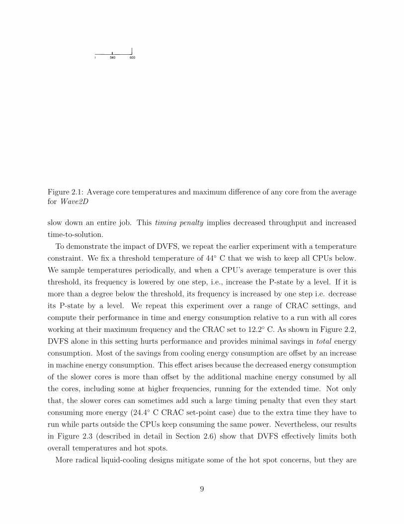
Figure 2.1: Average core temperatures and maximum difference of any core from the averagefor Wave2D
slow down an entire job. This timing penalty implies decreased throughput and increased
time-to-solution.
To demonstrate the impact of DVFS, we repeat the earlier experiment with a temperature
constraint. We fix a threshold temperature of 44◦ C that we wish to keep all CPUs below.
We sample temperatures periodically, and when a CPU’s average temperature is over this
threshold, its frequency is lowered by one step, i.e., increase the P-state by a level. If it is
more than a degree below the threshold, its frequency is increased by one step i.e. decrease
its P-state by a level. We repeat this experiment over a range of CRAC settings, and
compute their performance in time and energy consumption relative to a run with all cores
working at their maximum frequency and the CRAC set to 12.2◦ C. As shown in Figure 2.2,
DVFS alone in this setting hurts performance and provides minimal savings in total energy
consumption. Most of the savings from cooling energy consumption are offset by an increase
in machine energy consumption. This effect arises because the decreased energy consumption
of the slower cores is more than offset by the additional machine energy consumed by all
the cores, including some at higher frequencies, running for the extended time. Not only
that, the slower cores can sometimes add such a large timing penalty that even they start
consuming more energy (24.4◦ C CRAC set-point case) due to the extra time they have to
run while parts outside the CPUs keep consuming the same power. Nevertheless, our results
in Figure 2.3 (described in detail in Section 2.6) show that DVFS effectively limits both
overall temperatures and hot spots.
More radical liquid-cooling designs mitigate some of the hot spot concerns, but they are
9

0
100
200
300
400
500
NoLB 14.4 17.8 21.1 24.4 0
200
400
600
800
1000
1200
1400
Tim
e (
se
c)
En
erg
y (
KJ)
CRAC Set Point (C)
TimeMachine EnergyCooling Energy
Figure 2.2: Execution time and energy consumption for Wave2D running at different CRACset-points using DVFS
not a panacea. Equipment must be specifically designed to be liquid-cooled, and data centers
must be built or retrofit to supply the coolant throughout the machine room. The present
lack of commodity liquid-cooled systems and data centers means that techniques to address
the challenges of air-cooled computers will continue to be relevant for the foreseeable future.
Moreover, our techniques for limiting core temperatures can actually reduce the overall
thermal load of an HPC system, leading to energy savings even for installations using liquid
cooling.
2.3 Charm++ and Load Balancing
Charm++ is a general-purpose C++-based parallel programming system designed for pro-
ductive HPC programming [29]. It is supported by an adaptive runtime system that au-
tomates resource management. It relies on techniques such as processor virtualization and
over-decomposition (having more work units than the number of cores) to improve perfor-
mance via adaptive overlap of computation and communication and data-driven execution.
The automated resource management implies that the developer does not need to program
in terms of the physical cores, but instead divides the work into pieces with a suitable grain
size to let the system manage them easily.
A key feature of Charm++ is that the units of work decomposition are migratable objects.
10

The adaptive runtime system can assign these objects to any processor and move them
around during program execution, for purposes including load balancing, communication
optimization, and fault tolerance. To enable effective load balancing, it tracks statistics of
each object’s execution, including its computation time and communication volume [30].
The runtime system provides a variety of plug-in load balancing strategies that can account
for different application characteristics. Through a simple API, these strategies take the
execution statistics from the runtime and generate a set of migration instructions, describing
which objects to move between which processors. Application developers and users can
provide their own strategy implementations as desired. Load balancing strategies can be
chosen at compilation or run-time. The majority of these strategies are based on the heuristic
‘principle of persistence’, which states that each object’s computation and communication
loads tend to persist over time. The principle of persistence holds for a large class of iterative
HPC applications. In this study, we have developed a new load balancing strategy that
accounts for the performance effects of DVFS-induced heterogeneity. The new strategy is
described in detail in Section 2.4.
At small scales, the cost of the entire load balancing process, from instrumentation through
migration, is generally a small portion of the total execution time, and less than the improve-
ment that it provides. For cases where load balancing costs can be significant, a strategy
must be chosen or adapted to match the application’s needs [31]. Our approach can be eas-
ily adapted to available hierarchical schemes, which have been shown to scale to the largest
machines available [32]. By limiting the cost of decision-making and scope of migration, we
expect these schemes to offer similar energy benefits.
2.3.1 AMPI
The Message Passing Interface (MPI) is a standardized communication library for distributed-
memory parallel programming. MPI has become the dominant paradigm for large-scale par-
allel computing. Thus, techniques for addressing the energy consumption of large parallel
systems must be applicable to MPI applications.
Charm++ provides an implementation of MPI known as Adaptive MPI (AMPI). AMPI
makes the features of the Charm++ runtime system available to MPI programs. Common
MPI implementations implement each unit of parallel execution, or rank, as a separate
process. Pure MPI applications run one rank per CPU core, while others use fewer ranks
and gain additional shared-memory parallelism via threading.
In contrast, AMPI encourages running applications with several ranks per core. AMPI
11

implements these ranks as light weight user-level threads, many of which can run in each
process. The runtime schedules these threads non-preemptively, and switches them when
they make blocking communication calls. Internally, these threads are implemented as mi-
gratable objects, enabling the same benefits for MPI programs as for native Charm++.
In particular, AMPI allows us to apply the Charm++ load balancing strategies without
intrusive modifications to application logic.
2.4 ‘Cool’ Load Balancer
In this section, we introduce a novel approach that reduces energy consumption of the system
with minimal timing penalty. It is based on limiting core temperatures using DVFS and task
migration. Because our scheme is tightly coupled to task migration, we chose Charm++ and
AMPI as our parallel programming frameworks as they allow easy task (object) migration
with low overhead. All implementations and experiments were done using Charm++ and
AMPI. However, our techniques can be applied to any parallel programming system that
provides efficient task migration.
The steps of our temperature-control scheme can be summarized as applying the following
process periodically:
1. Check the temperatures of all cores
2. Apply DVFS to cores that are hotter or colder than desired
3. Address the load imbalance caused by DVFS using our load balancer, TempLDB :
(a) Normalize task and core load statistics to reflect old and new frequencies
(b) Identify overloaded or underloaded cores
(c) Move work from overloaded cores to underloaded cores
The remainder of this section describes this process in detail.
Our temperature control scheme is periodically triggered after equally spaced intervals in
time, referred to as steps. Other DVFS schemes [23] try to react directly to the demands
of the application workload, and thus must sample conditions and make adjustments at
intervals on the order of milliseconds. In contrast, our strategy only needs to react to much
slower shifts in chip temperature, which occur over intervals of seconds. At present, DVFS
is triggered as part of the runtime’s load balancing infrastructure at a user-specified period.
12

Variable Description
n number of tasks in applicationp number of coresTmax maximum temperature allowedk current load balancing stepCi set of cores on same chip as core itaskT imeki execution time of task i during
step k (in ms)coreT imeki time spent by core i executing tasks
during step kfki frequency of core i during step k (in Hz)mk
i core number assigned to task iduring step k
{task, core}Tickski num. of clock ticks taken by ith task/coreduring step k
tki average temperature of chip i at start ofstep k (in ◦C)
overHeap heap of overloaded coresunderSet set of underloaded cores
Table 2.1: Description for variables used in Algorithm 1
Our control strategy for DVFS is to let the cores work at their maximum frequency as
long as their temperature is below a threshold parameter. If a core’s temperature crosses
above the threshold, it is controlled by decreasing the voltage and frequency using DVFS.
When the voltage and frequency are reduced, power consumption will drop and hence the
core’s temperature will fall. Our earlier approach [33] raised the voltage and frequency as
soon as temperatures fell below the threshold, causing frequent changes and requiring effort
to load balance in every interval. To reduce overhead, our strategy now waits until a chip’s
temperature is a few degrees below the threshold before increasing its frequency.
The hardware in today’s cluster computers does not allow reducing the frequency of each
core individually and so we must apply DVFS to the whole chip. This raises the question:
what heuristic should we use to trigger DVFS and modulate frequency? In our earlier
work [15], we conducted DVFS when any of the cores on a chip were considered too hot.
However, our more recent results [33] show that basing the decision on average temperature
of the cores in a chip results in better temperature control.
Another important decision is how much a chip’s frequency should be reduced (respec-
tively, raised) when it gets too hot (is safe to warm up). Present hardware only offers discrete
frequency and voltage levels built into the hardware, the ‘P-states’. Using this hardware, we
observed that reducing the chip’s frequency by one level at a time is a reasonable heuristic
because it effectively constrains the core temperatures in the desired range (Figure 2.3).
Lines 1–6 of Algorithm 1 apply DVFS as we have just described. The description of the
13

variables and functions used in the algorithm is given in Table 2.1.
When DVFS adjusts frequencies differently across the cores in a cluster, the workloads on
those cores change relative to one another. Because this potential for load imbalance occurs
all at once, it makes sense to react to this load balance immediately. The system responds
by rebalancing the assignment of work to cores according to the strategy described by lines
7–32 of Algorithm 1.
Algorithm 1: Temperature Aware Refinement Load Balancing
1: On every node i at start of step k2: if tki > Tmax then3: decreaseOneLevel(Ci) . increase P-state4: else if tki < Tmax − 2 then5: increaseOneLevel(Ci) . decrease P-state6: end if7: On Master core8: for i ∈ [1, n] do9: taskT icksk−1i = taskT imek−1i × fk−1
mk−1i
10: totalT icks += taskT icksk−1i
11: end for12: for i ∈ [1, p] do13: coreT icksk−1i = coreT imek−1i × fk−1i
14: freqSum += fki15: end for16: createOverHeapAndUnderSet()17: while overHeap NOT NULL do18: donor = deleteMaxHeap(overHeap)19: (bestTask, bestCore) =20: getBestCoreAndTask(donor, underSet)21: mk
bestTask = bestCore22: coreT icksk−1donor− = taskT icksk−1bestTask
23: coreT icksk−1bestCore+ = taskT icksk−1bestTask
24: updateHeapAndSet()25: end while26:
27: procedure isHeavy(i)28: return coreT icksk−1i > (1 + tolerance) ∗ totalT icks29: ∗(fki /freqSum)30:
31: procedure isLight(i)32: return coreT icksk−1i < totalT icks ∗ fki /freqSum
The key principle in how a load balancer must respond to DVFS actuation is that the
14

load statistics must be adjusted to reflect the various different frequencies at which load
measurements were recorded and future work will run. At the start of step k, our load
balancer retrieves load information for step k−1 from Charm++’s database. This data gives
the total duration of work executed for each task in the previous interval (taskT imek−1i ) and
the core that executed it (mk−1i ). Here i refers to task id and k − 1 represents last step.
We normalize the task workloads by multiplying their execution times by the old frequency
values of the core that hosted them. We then sum these normalized task workloads to
compute the total load, as seen in lines 8–11. This normalization is an approximation to
the performance impact of different frequencies. However, different applications might have
different characteristics (e.g., cache hit rates at various levels, instructions per cycle) that
determine the sensitivity of their execution time to core frequency. We plan to incorporate
more detailed load estimators in our future work. The scheme also calculates the work
assigned to each core and sum of frequencies for all the cores to be used later (lines 12-15).
Once the load normalization is done, we create a max heap for overloaded cores (overHeap)
and a set for the underloaded cores (underSet) on line 16. The cores are classified as
overloaded and underloaded by procedures isHeavy() and isLight() (lines 26–30), based on
how their normalized loads from the previous step, k−1, compare to the frequency-weighted
average load for the coming step k. We use a tolerance in identifying overloaded cores to
focus our efforts on the worst instances of overload and minimize migration costs. In our
experiments, we set the tolerance to 0.07, empirically chosen for the slight improvement that
it provided over the lower values used in our previous work.
Using these data structures, the load balancer iteratively moves work away from the most
overloaded core (donor, line 18) until none are left (line 17). The moved task and recipient
are chosen as the heaviest task that the donor could transfer to any underloaded core such
that the underloaded core does not become overloaded (line 19, implementation not shown).
Once the chosen task is reassigned (line 20), the load statistics are updated and the data
structures are updated accordingly (lines 21–23).
2.5 Experimental Setup
To evaluate our approach to reducing energy consumption, we must be able to measure
and control core frequencies and temperatures, air temperature, and energy consumed by
computer and cooling hardware. All experiments were run on real hardware and this chapter
does not include any simulation results.
We tested our scheme on the Energy Cluster hosted by the Computer Science department
15

at University of Illinois Urbana Champaign (see Appendix A). Its cooling design is similar
to the cooling systems of most large data centers. We were able to vary the CRAC set-point
across a broad range as shown in our results (following sections).
Because the CRAC unit exchanges machine room heat with chilled water supplied by a
campus-wide plant, measuring its direct energy consumption (i.e., with an electrical meter)
would only include the mechanical components driving air and water flow, and would miss
the much larger energy expenditure used to cool the water. To capture the machine room’s
cooling energy, we use a model [21] based on measurements of how much heat the CRAC
actually expels. The instantaneous power consumed by the CRAC to cool the temperature
of the exhaust air from Thot down to the cool inlet air temperature Tac can be approximated
by:
Pac = cair ∗ fac ∗ (Thot − Tac) (2.1)
In this equation, cair is the heat capacity constant and fac is the constant rate of air flow
through the cooling system. We use temperature sensors on the CRAC’s vents to measure
Thot and Tac. During our experiments, we recorded a series of measurements from each of
these sensors, and then integrated the calculated power to produce total energy figures.
By working in a dedicated space, the present work removes a potential source of error from
previous data center cooling results. Most data centers have many different jobs running
at any given time. Those jobs dissipate heat, interfering with cooling energy measurements
and increasing the ambient temperature in which the experimental nodes run. In contrast,
our cluster is the only heat source in the space, and the CRAC is the primary sink for that
heat.
We investigate the effectiveness of our scheme, using five different applications, of which
three are Charm++ applications and two are written in MPI. These applications have a
range of power profiles and are described in Appendix B.
Most of our experiments were run for 300 seconds as it provided ample time for all ap-
plications to settle to their steady state frequencies. All results that we show are averaged
over three identically configured runs, with a cool-down period before each. All normalized
results are reported with respect to a run where all 128 cores were running at the maximum
possible frequency with Intel Turbo Boost in operation and the CRAC set to 12.2◦ C. To
validate the ability of our scheme to reduce energy consumption for longer execution times,
we ran Wave2D (the most power-hungry of the five applications we consider) for 2.5 hours.
The longer run was consistent with our findings, with the temperature being constrained
well within the specified range and we were able to reduce cooling energy consumption for
the entire 2.5 hour period.
16

2.6 Constraining Core Temperatures and Timing Penalty
The approach that we have described in Section 2.4 constrains processor temperatures with
DVFS while attempting to minimize the resulting timing penalty. Figure 2.3 shows that all
of our applications when using DVFS and TempLDB, settle to an average temperature that
lies in the desired range (the two horizontal lines at 47 ◦C and 49 ◦C on Figure 2.3). As the
average temperature increases to its steady-state value, the hottest single core ends up no
more than 6◦ C above the average (lower part of Figure 2.3) as compared to 20◦ C above
average for the run where we are not using temperature control (Figure 2.1).
Figure 2.4 shows the timing penalty incurred by each application under DVFS, contrasting
its effect with and without load balancing. The effects of DVFS on the various applications
are quite varied. The worst affected, Wave2D and NAS MG, see penalties of over 50%, which
load balancing reduces to below 25%. Jacobi2D was the least affected, with a maximum
penalty of 12%, brought down to 3% by load balancing. In all cases, the timing penalty
sharply decreases when load balancing is activated, generally by greater than 50%. Before
analyzing the timing penalty for individual applications we first see how load balancing helps
in reducing timing penalty compared to naive DVFS.
To illustrate the benefits of load balancing, we use Projections [34], which is a multipurpose
performance visualization tool for Charm++ applications. Here, we use processor timelines
to see the utilization of the processors in different time intervals. For ease of comprehension,
we show a representative 16-core subset of the 128-core cluster. The top part of Figure 2.5
shows the timelines for execution of Wave2D with the naive DVFS scheme. Each timeline
(horizontal line) corresponds to the course of execution of one core visualizing its utilization.
The green and pink colored pieces show different computation but white ones represent idle
time. The boxed area in Figure 2.5 shows some of the cores have significant idle time.
The top 4 cores in the boxed area take much longer to execute their computation than
the bottom 12 cores which is why the pink and green parts are longer for the top 4 cores.
However, the other 12 cores execute their computation quickly and stay idle waiting for the
rest of cores. The idle time is caused because DVFS decreased the frequency of the first
four cores and so they are slower in their computation. It means that the timing penalty
of naive DVFS is dictated by the slowest cores. The bottom part of Figure 2.5 shows the
same temperature control but using our TempLDB. In this case, there is no significant idle
time because the scheme balances the load between slow and fast processors by taking their
frequencies into account. Consequently, the latter approach results in much shorter total
execution time, as reflected by shorter timelines (and figure width) in the bottom part of
Figure 2.5. Now we try to understand the timing penalty differences amongst different
17

30
35
40
45
50
50 100 150 200
Tem
pera
ture
(C)
Cluster Average Temperature
Wave2DNPB-FT
NPB-MGMol3D
Jacobi2DAllowed range
0 2 4 6 8
10
50 100 150 200
Tem
pera
ture
dev
iatio
n (C
)
Time (s)
Highest Single-core Deviation from Cluster Average Temperature
Figure 2.3: Our DVFS and load balancing scheme successfully keeps all processors withinthe target temperature range of 47◦–49◦ C, with a CRAC set-point of 24.4◦ C.
applications by examining more detailed data. Jacobi2D experiences the lowest impact of
DVFS, regardless of load balancing (Figure 2.4(a)). The small timing penalty for Jacobi2D
occurs for several interconnected reasons. From the high level, Figure 2.3 shows that it takes
the longest of any application to increase temperatures to the upper bound of the acceptable
range, where DVFS activates. This slow ramp-up in temperature means that its frequency
does not drop until later in the run, and then falls relatively slowly, as seen in Figure 2.6
which plots the minimum frequency at which any core was running (Figure 2.6(a)) and
the average frequency (Figure 2.7(a)) for all 128 cores. Even when some processors reach
their minimum frequency, Figure 2.7(a) shows that its average frequency decreases more
slowly than any other application, and does not fall as far. The difference in the average
frequency and the minimum frequency explains the difference between TempLDB and naive
DVFS, as the execution time for TempLDB is dependent on average frequency whereas the
execution time for naive DVFS depends on the minimum frequency at which any core is
running. Another way to understand the relatively small timing penalty of Jacobi2D is
to compare its utilization and frequency profiles. Figure 2.8(a) depicts each core’s average
18

0
10
20
30
40
50
60
70
14.4 17.8 21.1 24.4
Tim
ing
Pen
alty
(%)
CRAC Set Point (C)
Naive DVFSTempLDB
(a) Jacobi2D
0
10
20
30
40
50
60
70
14.4 17.8 21.1 24.4
Tim
ing
Pen
alty
(%)
CRAC Set Point (C)
Naive DVFSTempLDB
(b) Wave2D
0
10
20
30
40
50
60
70
14.4 17.8 21.1 24.4
Tim
ing
Pen
alty
(%)
CRAC Set Point (C)
Naive DVFSTempLDB
(c) Mol3D
0
10
20
30
40
50
60
70
14.4 17.8 21.1 24.4
Tim
ing
Pen
alty
(%)
CRAC Set Point (C)
Naive DVFSTempLDB
(d) NPB-MG
0
10
20
30
40
50
60
70
14.4 17.8 21.1 24.4
Tim
ing
Pen
alty
(%)
CRAC Set Point (C)
Naive DVFSTempLDB
(e) NPB-FT
Figure 2.4: Execution timing penalty with and without Temperature Aware LoadBalancing
19

Figure 2.5: Execution timelines before and after Temperature Aware Load Balancing forWave2D
frequency over the course of the run. Figure 2.9(a) shows the utilization of each core while
running Jacobi2D. In both figures, each bar represents the measurement of a single core.
The green part of the utilization bars represents computation and the white part represents
idle time. As can be seen, utilizations of the right half cores are roughly higher than the left
half. Furthermore, the average frequency of the right half processors is roughly lower than
the other half. Thus, lower frequency has resulted in higher utilization of those processors
without much timing penalty. The reason this variation can occur is that the application
naturally has some slack time in each iteration, which the slower processors dip into to keep
pace with faster ones.
To examine the differences among applications at another level, Figure 2.10 shows the
performance impact of running each application with the processor frequencies fixed at a
particular value (the marking 2.4+ refers to the top frequency plus Turbo Boost). All ap-
plications slow down as CPU frequency decreases. However, Jacobi2D incurs the smallest
timing penalty compared to other applications. This marked difference can be better under-
stood in light of the performance counter-based measurements shown in Table 2.2. These
20

1.2
1.4
1.6
1.8
2
2.2
2.4
0 50 100 150 200 250 300
Min
imum
Fre
quen
cy (G
Hz)
Time (s)
Mol3DMG
Wave2DFT
Jacobi2D
Figure 2.6: Minimum core frequencies produced by DVFS for different applications at 24.4◦
C
1.2
1.4
1.6
1.8
2
2.2
2.4
0 50 100 150 200 250 300
Ave
rage
Fre
quen
cy (G
Hz)
Time (s)
Mol3DMG
Wave2DFT
Jacobi2D
Figure 2.7: Average core frequencies produced by DVFS for different applications at 24.4◦
C
Counter Type Jacobi2D Mol3D Wave2D
MFLOP/s 373 666 832Traffic L1-L2 (MB/s) 762 1017 601Cache misses to DRAM 663 75 402(millions)
Table 2.2: Performance counters for Charm++ applications on one core
21

0
0.5
1
1.5
2
0 20 40 60 80 100 120
Ave
rag
e F
req
ue
ncy
Core Number
Figure 2.8: Average frequency of processors for Jacobi2D using TempLDB
Figure 2.9: Utilization of processors for Jacobi2D using TempLDB
22

measurements were taken in equal-length runs of the three Charm++ applications using
the PerfSuite toolkit [35]. Jacobi2D has a much lower computational intensity, in terms of
FLOP/s, than the other applications. It also retrieves much more data from main memory,
explaining its lower sensitivity to frequency shifts. Its lower intensity also means that it
consumes less power and dissipates less heat in the CPU cores than the other applications,
explaining its slower ramp-up in temperature, slower ramp-down in frequency, and higher
steady-state average frequency. In contrast, the higher FLOP counts and cache access rates
of Wave2D and Mol3D explain their high frequency sensitivity, rapid core heating, lower
steady-state frequency, and hence the large impact DVFS has on their performance.
0.8
0.9
1
1.1
1.21.41.61.822.22.42.4+
Nor
mal
ized
Thr
ough
put
Frequency (GHz)
NPB-MGMol3D
NPB-FTWave2D
Jacobi2D
Figure 2.10: Frequency sensitivity of the various applications
2.7 Energy Savings
In this section, we evaluate the ability of our scheme to reduce total energy consumption. Our
current load balancing scheme with the allowed temperature range strategy resulted in less
than 1% time overhead for applying DVFS and load balancing (including the cost of object
migration). Due to that change, we now get savings in both cooling energy consumption
as well as machine energy consumption, although savings in cooling energy consumption
constitute the main part of the reduction in total energy consumption. In order to understand
the contribution for both cooling energy consumption and machine energy consumption, we
look at them separately.
23

2.7.1 Cooling energy consumption
The essence of our work is to reduce cooling energy consumption by constraining core tem-
peratures and avoiding hot spots. As outlined in Equation 2.1, the cooling power consumed
by the air conditioning unit is proportional to the difference between the hot air and cold
air temperatures going in and out of the CRAC respectively. As mentioned in earlier work
[4–6], cooling cost can be as high as 50% of the total energy budget of the data center. How-
ever, in our calculation, we take it to be 40% of the total energy consumption of a baseline
run with the CRAC at its lowest set-point, which is equivalent to 66.6% of the measured
machine energy during that run. Hence, we use the following formula to estimate the cooling
power by feeding in actual experimental results for hot and cold air temperatures:
PLBcool =
2 ∗ (TLBhot − TLBac ) ∗ P basemachine
3 ∗ (T basehot − T baseac )(2.2)
TLBhot represents the temperature of hot air leaving the machine room (entering the CRAC)
and TLBac represents the temperature of the cold air entering the machine room. T basehot and
T baseac represent the hot and cold air temperatures with the largest difference while running
Wave2D at the coolest CRAC set-point (i.e., 12.2◦ C), and P basemachine is the power consumption
of the machine for the same experiment.
Figure 2.11 shows the machine power consumption and the cooling power consumption for
each application using TempLDB. Figure 2.11(b) shows that the cooling power consumption
falls as we increase the CRAC set-point for all applications. A higher CRAC set-point means
the cores heat up more rapidly, leading DVFS to set lower frequencies. Thus, machine
power consumption falls as a result of the CPUs drawing less power (Figure 2.11(a)). The
machine’s decreased power draw and subsequent heat dissipation means that less energy is
added to the machine room air. The lower heat flux to the ambient air means that the
CRAC requires less power to expel that heat and to maintain the set-point temperature, as
seen in Figure 2.11(b).
Wave2D consumes the highest cooling power for three out of the four CRAC set-points
that we used, which is consistent with its high machine power consumption. Figure 2.12
shows the savings in cooling energy in comparison to the baseline run where all cores are
working at the maximum frequency without any temperature control. These figures include
the extra time that the cooling needs to run corresponding to the timing penalty introduced
because of applying DVFS. Due to the large reduction in cooling power (Figure 2.11(b))
our scheme was able to save as much as 63% of the cooling energy in the case of Mol3D
running at a CRAC set-point of 24.4 ◦C. We can see that the savings in cooling energy
24

0
500
1000
1500
2000
2500
3000
3500
4000
4500
No DVFS 14.4°C 17.8°C 21.1°C 24.4°C
Mac
hine
Pow
er (W
)
CRAC Temperature
Mol3DJacobi
NPB-MGNPB-FTWave2D
(a) Machine power consumption
0
500
1000
1500
2000
2500
3000
3500
4000
4500
No DVFS 14.4°C 17.8°C 21.1°C 24.4°C
Coo
ling
Pow
er (W
)
CRAC Temperature
Mol3DJacobi
NPB-MGNPB-FTWave2D
(b) Cooling power consumption
Figure 2.11: Machine and cooling power consumption for no-DVFS runs at a 12.2 ◦C set-point and various TempLDB runs
25

consumption are better with our technique than naive DVFS for most of the applications
and the corresponding set-points. This improvement in energy consumption is mainly due
to the higher timing penalty for naive DVFS runs, which causes the CRAC to work for much
longer than the corresponding TempLDB run.
2.7.2 Machine energy consumption
Although TempLDB does not optimize for reduced machine energy consumption, we still end
up showing savings for some applications. Figure 2.13 shows the change in machine energy
consumption. A number less than 1 represents a saving in machine energy consumption
whereas a value greater than 1 points to an increase.
It is interesting to see that NPB-FT and Wave2D end up saving machine energy con-
sumption when using TempLDB. For Wave2D, we end up saving 6% of machine energy
consumption when the CRAC is set to 14.4 ◦C whereas the maximum machine energy sav-
ings of NPB-FT, 4%, occurs when the CRAC is set to 14.4 ◦C or 24.4 ◦C. To find the reasons
for these savings in machine energy consumption, we performed a set of experiments where
we ran the applications with the 128 cores of our cluster fixed at each of the available fre-
quencies. Figure 2.14 plots the normalized machine energy for each application against the
frequency at which it was run. Power consumption models dictate that CPU power con-
sumption can be regarded as being proportional to the cube of the frequency, which would
imply that we should expect the power to fall as a cubic of frequency whereas the execution
time increases only linearly in the worst case. This cubic relationship would imply that we
should always reduce energy consumption by moving to a lower frequency. This proposition
does not hold because of the high base power drawn by everything other than the CPU and
memory subsystem, which is 40W per node for our cluster. We can say that while moving
to each successive lower frequency we reach a point where the savings in the CPU energy
consumption are offset by an increase in base energy consumption due to the timing penalty
incurred, leading to the U-shaped energy curves. When our scheme lowers frequency as a
result of core temperature crossing the maximum temperature value, we move into the more
desirable range of machine energy consumption, i.e., closer to the minimum of the U-shape
energy curves.
To see a breakdown of execution time, Figure 2.15 shows the cumulative time spent by
all 128 cores at different frequency levels for Wave2D using TempLDB at a CRAC set-
point of 24.4 ◦C. We can see that most of the time is spent at frequency levels between
1.73GHz–2.0GHz, which corresponds to the lowest point for normalized energy for Wave2D
26

0
10
20
30
40
50
60
70
14.4 17.8 21.1 24.4
Savin
gs in C
oolin
g E
nerg
y (
%)
CRAC Set Point (C)
Naive DVFSTempLDB
(a) Jacobi2D
0
10
20
30
40
50
60
70
14.4 17.8 21.1 24.4
Savin
gs in C
oolin
g E
nerg
y (
%)
CRAC Set Point (C)
Naive DVFSTempLDB
(b) Wave2D
0
10
20
30
40
50
60
70
14.4 17.8 21.1 24.4
Savin
gs in C
oolin
g E
nerg
y (
%)
CRAC Set Point (C)
Naive DVFSTempLDB
(c) Mol3D
0
10
20
30
40
50
60
70
14.4 17.8 21.1 24.4
Savin
gs in C
oolin
g E
nerg
y (
%)
CRAC Set Point (C)
Naive DVFSTempLDB
(d) NPB-MG
0
10
20
30
40
50
60
70
14.4 17.8 21.1 24.4
Savin
gs in C
oolin
g E
nerg
y (
%)
CRAC Set Point (C)
Naive DVFSTempLDB
(e) NPB-FT
Figure 2.12: Savings in cooling energy consumption with and without Temperature AwareLoad Balancing (higher is better)
27

0
0.2
0.4
0.6
0.8
1
1.2
1.4
1.6
14.4 17.8 21.1 24.4
Norm
aliz
ed M
achin
e E
nerg
y
CRAC Set Point (C)
Naive DVFSTempLDB
(a) Jacobi2D
0
0.2
0.4
0.6
0.8
1
1.2
1.4
1.6
14.4 17.8 21.1 24.4
Norm
aliz
ed M
achin
e E
nerg
y
CRAC Set Point (C)
Naive DVFSTempLDB
(b) Wave2D
0
0.2
0.4
0.6
0.8
1
1.2
1.4
1.6
14.4 17.8 21.1 24.4
Norm
aliz
ed M
achin
e E
nerg
y
CRAC Set Point (C)
Naive DVFSTempLDB
(c) Mol3D
0
0.2
0.4
0.6
0.8
1
1.2
1.4
1.6
14.4 17.8 21.1 24.4
Norm
aliz
ed M
achin
e E
nerg
y
CRAC Set Point (C)
Naive DVFSTempLDB
(d) NPB-MG
0
0.2
0.4
0.6
0.8
1
1.2
1.4
1.6
14.4 17.8 21.1 24.4
Norm
aliz
ed M
achin
e E
nerg
y
CRAC Set Point (C)
Naive DVFSTempLDB
(e) NPB-FT
Figure 2.13: Change in machine energy consumption with and without Temperature AwareLoad Balancing (values less than 1 represent savings)
28

in Figure 2.14.
In order to study the relationship between machine power consumption and average fre-
quency we plotted the power consumption for each application over the course of a run using
TempLDB in Figure 2.16. It was counter intuitive to see that despite starting at the same
level of machine power consumption as NPB-FT and NPB-MG, Jacobi2D ended up having
a much higher average frequency (Figure 2.7(a)). The other interesting observation that we
can make from this graph is the wide variation in steady state power consumption among
the applications.
Since all the applications are settling to the same average core temperature, the laws of
thermodynamics dictate that a CPU running at a fixed temperature will transfer a particular
amount of heat energy per unit of time to the environment through its heatsink and fan
assembly. Thus, each application should end up having the same CPU power consumption.
Similar CPU power consumption would mean that the difference in power draw among the
applications in Figure 2.16 is caused by something other than CPU power consumption.
Table 2.2 shows that Jacobi2D and Wave2D have many more cache misses than Mol3D and
thus end up with a higher power consumption in the memory controller and DRAM, which
do not contribute to increased core temperatures but do increase the total power draw for
the machine.
In order to verify our hypothesis, we ran two of our applications, Jacobi2D and Wave2D,
on a single node containing a 4-core Intel Core i7-2600K, with a temperature threshold of
50◦C. Using our load balancing infrastructure and the newly added hardware energy counters
in Intel’s recent Sandy Bridge technology present in this chip, we can measure the chip’s
power consumption directly from machine specific registers using Running Average Power
Limit (RAPL) library [36]. Both applications begin execution with the CPU at its maximum
frequency, which our system decreases as temperatures rise.
The CPU power consumption results from these runs are graphed in figure 2.17. As
expected, both applications settled near a common steady state of power consumption for
the CPU package (cores and caches combined).
Before highlighting the key findings of our study, we compare our load balancer, i.e.,
TempLDB, with a generic Charm++ load balancer, i.e., RefineLDB. RefineLDB ’s load bal-
ancing strategy relies on execution time data for each task without taking into account the
frequency at which each core is working. Similar to TempLDB, RefineLDB also migrates
extra tasks from the overloaded cores to the underloaded cores. We implemented our tem-
perature control scheme using DVFS into this load balancer but kept the load balancing
part the same. Because RefineLDB relies only on task execution time data to predict future
load without taking into account the transitions in core frequencies, it ends up taking longer
29

0.8
0.9
1
1.1
1.2
1.21.41.61.822.22.42.4+
Nor
mal
ized
Ene
rgy
Frequency (GHz)
Wave2DNPB-FT
NPB-MGMol3D
Jacobi2D
Figure 2.14: Normalized machine energy consumption for different frequencies using 128cores
4000
8000
12000
16000
2.4
0+
2.4
0
2.2
6
2.1
3
2.0
0
1.8
6
1.7
3
1.6
0
1.4
6
1.3
3
1.2
0Ti
me
(s)
Frequency (GHz)
Figure 2.15: The time Wave2D spent in different frequency levels
30

2400
2600
2800
3000
3200
3400
3600
50 100 150 200 250 300 350 400
Clu
ster
Pow
er (W
)
Time (sec)
Jacobi2DWave2DNPB-FT
Mol3DNPB-MG
Figure 2.16: Total power draw for the cluster using TempLDB at CRAC set-pointof 24.4 ◦C
0
10
20
30
40
50
60
0 50 100 150 200 250 300 350 400
Pow
er (W
)
Time (s)
Jacobi Package PowerWave2d Package Power
Figure 2.17: Power consumption of two applications as their DVFS settings stabilize to asteady state
31

0
5
10
15
20
25
30
35
Wave2D MG Mol3D FT Jacobi2DTim
ing
Pen
alty
/ E
nerg
y S
avin
gs (%
)
RefineLDB TimeTempLDB Time
RefineLB Total EnergyTempLDB Total Energy
Figure 2.18: Timing penalty and energy savings of TempLDB and RefineLDB compared tonaive DVFS
and consumes more energy to restore load balance. The improvement that TempLDB makes
can be seen from Figure 2.18 which shows a comparison between both load balancers for all
applications with the CRAC set-point at 22.2◦C.
2.8 Tradeoff in Execution Time and Energy Consumption
The essence of our results can be seen in Figure 2.19, which summarizes the tradeoffs between
execution time and total energy consumption for all five applications. Each application
has two curves, one for each of the Naive DVFS and TempLDB runs. These curves give
important information: the slope of each curve represents the execution time penalty one
must pay in order to save each joule of energy. A movement to the left (reducing the
energy consumption) or down (reducing the timing penalty) is desirable. For all CRAC
set-points across all applications, TempLDB takes its corresponding point from the Naive
DVFS scheme at the same CRAC set-point down (saving timing penalty) and to the left
(saving energy consumption).
From Figure 2.19(b), we can see that Wave2D is only conducive to saving energy with
the CRAC set below 21.1◦ C, as the curve becomes vertical with higher set-points. However
we should note that the temperature range of 47 ◦C–49 ◦C was much lower than the average
temperature Wave2D reached with the CRAC set at the coolest set-point of 12.2◦ C without
any temperature control. Thus, a higher CRAC set-point imposes too much timing penalty
to provide any total energy savings beyond the 21.1◦ C set-point. Even at 14.4◦ C we
32

1
1.02
1.04
1.06
1.08
1.1
1.12
1.14
1.16
0.8 0.85 0.9 0.95 1 1.05
Norm
aliz
ed T
ime
Normalized Energy
14.4°C17.8°C
21.1°C
24.4°C
14.4°C
17.8°C
21.1°C
24.4°C
TempLDBNaive DVFS
(a) Jacobi2D
1.05
1.1
1.15
1.2
1.25
1.3
1.35
1.4
1.45
0.85 0.9 0.95 1 1.05 1.1 1.15
Norm
aliz
ed T
ime
Normalized Energy
14.4°C
17.8°C
21.1°C
14.4°C
17.8°C
21.1°C
24.4°C
TempLDBNaive DVFS
(b) Wave2D
1
1.05
1.1
1.15
1.2
1.25
1.3
1.35
1.4
1.45
0.7 0.75 0.8 0.85 0.9 0.95 1 1.05 1.1 1.15
Norm
aliz
ed T
ime
Normalized Energy
14.4°C
17.8°C
21.1°C
24.4°C 14.4°C
17.8°C
21.1°C
24.4°C
TempLDBNaive DVFS
(c) Mol3D
1
1.05
1.1
1.15
1.2
1.25
1.3
1.35
1.4
1.45
0.7 0.75 0.8 0.85 0.9 0.95 1 1.05 1.1 1.15
Norm
aliz
ed T
ime
Normalized Energy
14.4°C17.8°C
21.1°C
24.4°C
14.4°C17.8°C
21.1°C
TempLDBNaive DVFS
(d) NPB-MG
1
1.05
1.1
1.15
1.2
1.25
1.3
1.35
1.4
1.45
0.75 0.8 0.85 0.9 0.95 1 1.05
Norm
aliz
ed T
ime
Normalized Energy
14.4°C17.8°C
21.1°C
24.4°C14.4°C
17.8°C
21.1°C
24.4°CTempLDBNaive DVFS
(e) NPB-FT
Figure 2.19: Normalized time against normalized total energy for a representative subset ofapplications
33

are able to reduce its total energy consumption by 12%. The benefits of using TempLDB
will eventually end for any application, i.e., the curve will become vertical, as we keep on
increasing the CRAC set-point. However, the set-point at which the benefits end would
differ amongst different applications.
For Mol3D, the nearly flat curve shows that our scheme does well at saving energy, since
we do not have to pay a large execution time penalty in order to reduce energy consumption.
The same effect holds true for Jacobi2D. NPB-MG ’s sloped curve places it in between these
two extremes. It and NPB-FT truly present a tradeoff, and users can optimize according to
their preferences.
34
CHAPTER 3Thermal Restraint and Reliability
HPC research and its endeavor to build larger machines face several major challenges today
including, power, energy, and reliability. Petascale systems spend significant time dumping
checkpoint data to remote storage while executing large scientific applications. Although
these systems are built from highly reliable individual components, the overall failure rate
for them is high due to the shear number of components involved in building such large
machines. Current petascale machines have Mean Time Between Failures (MTBF) that can
be anywhere from a few hours to days [37]. These MTBF numbers could be significantly
smaller for an exascale machine as pointed out in Figure 1.1. Given the current per socket
MTBF values, the proposed exascale machine can have an MTBF of less than an hour!
Past research has shown a relation between core temperatures and reliability. The failure
rate of a compute node doubles with every 10◦ C increase in temperature [8,38–40]. This rule
is commonly known as the 10-degree rule. Most HPC researchers have focused on developing
efficient fault tolerance protocols in the past [41–44]. The work presented in this chapter
follows a different path. Instead of efficiently dealing with faults, we aim at reducing their
occurrence. Hence, our scheme can be beneficial when combined with any fault tolerance
protocol. In Chapter 2 we demonstrated the ability of thermal restraint to reduce total
energy consumption of a data center. We now extend the scheme proposed in Chapter 2 and
combine it with a checkpoint-restart protocol [41] to improve application performance in a
faulty environment. In this chapter we show that by restraining processor temperatures,
we can empower the user to select the reliability of the system from within a range. An
increase in reliability can improve the performance of an application especially by using
load balancing for overdecomposed systems [45]. We also show how different applications
can affect the Mean Time Between Failures (MTBF) for a machine due to different thermal
profiles. We present and analyze the tradeoffs of improving reliability and its associated cost,
35

i.e., the slowdown caused by DVFS-driven temperature control. In particular, this chapter
makes the following contributions:
• We analyze how restraining temperature of individual processors improves the relia-
bility of the entire machine (Section 3.2.1).
• We formulate a model that relates total execution time of an application to reliability
and the associated slowdown for temperature restraint (Section 3.2.2).
• We propose, implement and evaluate a novel approach that extends our earlier work [33,
46] and combines temperature restraint, load balancing and checkpoint/restart to in-
crease reliability while reducing total execution time for an application (Section 3.3).
We do several experiments that span over an hour and have at least 40 faults. This
work is, as far as we know, the first extensive experimental study that provides insights
on the effects of temperature restraint on estimated MTBF for HPC machines.
• We first validate the accuracy of our model (Section 3.4) and then use it to show the
scheme’s expected benefits for larger machines (Section 3.5). Our results show that
for a 340K socket machine, we improve the machine efficiency from 0.01 to 0.22 as a
result of improving the machine reliability by a factor of up to 2.29.
3.1 Related Work
The classical solution for coping with an ever increasing failure rate due to larger machine
sizes and thermal variations is to increase the checkpoint frequency. Unfortunately, check-
point/restart might not be usable indefinitely as the failure rate grows.
Some alternatives have been explored to keep up with a small MTBF . Using local storage
to store the state of the tasks has been proposed in the double in-memory checkpoint/restart
mechanism [41,47]. Checkpointing in the memory of the nodes is fast and checkpoint periods
can become smaller to tolerate frequent failures. Although this mechanism may not tolerate
the failure of more than one node, several studies have confirmed that in a high percentage
of the failures, only one node is affected [47, 48]. Another possibility is to improve recovery
time through message-logging. In such protocols, a failure only requires the crashed node to
roll back. The rest of the system will re-send the messages and wait for the crashed node
to catch up with the rest of the system. A technique called parallel recovery [49] leverages
message-logging by distributing the tasks on the failed node to be recovered in parallel on
other nodes of the system. This mechanism has been demonstrated to tolerate a higher
36

failure rate [50]. More recently, replication of tasks has been proposed to deal with high
failure rates [12]. However, replication decreases the utilization of the system to 50% at the
best. An extremely high failure rate will make this sacrifice pay off, as the utilization of a
system using checkpoint/restart drastically decreases if failures are very frequent.
In this dissertation, we take a different approach of dealing with faults. Instead of finding
efficient schemes that deal with faults, we aim to avoid failures by controlling tempera-
ture in all nodes of a system using DVFS. The net result of this temperature capping is a
smaller failure rate. We compensate for loss of performance due to DVFS with load bal-
ance and over-decomposition. A decreased failure rate is particularly more convenient for
checkpoint/restart, but our scheme can be used in tandem with any fault-tolerance method.
One of the key advantages of decreasing the failure rate is the reduction in maintenance
cost of the supercomputing facility. Each failure may require at least a reboot, but in some
situations manual intervention of experts is needed to diagnose the root cause of the crash.
3.2 Implications of Temperature Control
Processor temperature has a profound impact on the fault rate of a processor. For every
10◦ C increase in processor temperature the fault rate doubles [8, 38–40]. While restraining
processor temperature improves reliability, it also causes an execution time slowdown due to
DVFS. In this section, we use temperature control to estimate the improvement in reliability
and its impact on the total execution time of an application.
3.2.1 Effects of Temperature Control on Reliability
MTBF for a processor (m) is exponentially related to its temperature and can be expressed
as: [8–10]
m = A ∗ e−b∗T (3.1)
where T is the processor temperature, A and b are constants. Assuming an m of 10 years
at 40◦ C, m per processor based on the 10-degree rule can be expressed as:
m = 160 ∗ e−0.069T (3.2)
37

50 55 60 65 70 75 80 850
1
2
3
4
5
6
7
Num
ber
of pro
cessors
Processor temperature ( °C)
Cool Processors
Hot Processors
Figure 3.1: Histogram of max temperature for each node of the cluster using Wave2D
In a system where the failure of a single component can cause the entire application to fail,
the MTBF of the system can be defined as (M) [51]:
M =1∑N
n=11mn
(3.3)
where N is the number of nodes and mn is the MTBF for socket n. Although the absolute
value of core temperatures is important for each processor’s reliability (Equation 3.2), relia-
bility of the entire cluster also depends on the variance of core temperatures for all processors
present in the cluster (Equation 3.3). Presence of hot spots can degrade reliability of the
system.
To analyze processor temperature behavior, we ran a 5-point stencil application, Wave2D,
on a 32 node (128 cores) cluster for over 30 mins and recorded the maximum temperature
reached by each processor. The results are pictured in Figure 3.1 where each bar shows
the number of processors reaching a specific maximum temperature during the 30-min run.
The red bars in Figure 3.1 indicate the presence of a hot spot composed of three processors
(hot processors) that heated up to 78◦ C-80◦ C. The maximum temperature reached by the
remaining 29 processors (cold processors) ranged from 55◦ C-63◦ C (shown in blue). The
average temperature for the cool processors was Tc = 59◦ C, with a standard deviation of σ
= 2.17◦ C. Feeding the temperature data from Figure 3.1 to Equations 3.2 and 3.3 estimates
the MTBF to be 24 days for our cluster. As Equation 3.2 outlines, we can increase m for
each processor by restraining its temperature to a lower value and hence increase overall M
38

50 55 60 65 70 75 8020
25
30
35
40
45
50
55
60
0.5% (56°C)
4% (52°C)
1.5% (54°C)
Maximum allowed temperature ( °C)
MT
BF
of 32−
node c
luste
r (d
ays)
Figure 3.2: Effect of cooling down processors on MTBF of the system
for the cluster. To estimate the improvement in M , we do the following:
1. Remove the hot spot by bringing the hot processors’ distribution back to that of cool
processors
2. Shift the entire distribution towards the left so that all processors operate at an average
temperature of 50◦ C instead of 59◦ C
Suppose we remove the hot spot by restraining temperature for the three hot processors to
Tc = 59◦ C, i.e., the average temperature for cool processors. Using these new temperature
values for the three processors in the hot spot, along with the actual temperature values we
got for cool processors, we re-estimate M and notice an increase of 7 days (from 24 to 31
days). The estimated improvement in M after hot spot removal is shown by the dashed line
in Figure 3.2 which joins the two points representing the value of M with (red circle) and
without (blue diamond) hot spot. We can now predict M given a temperature restraint for
a processor in the hot spot. For example, keeping the three processors in the hot spot to
70◦ C would result in an estimated 27.5 days for M .
So far we have argued that hot spot removal improves M . Next, we study the effect of
restraining temperatures for all the processors to 50◦ C. For this, we generate 32 normally
distributed random temperature values with a mean of 50◦ C and σ = 2.17◦ C (same as
cool processors) and re-estimate M . The improvement in M for any temperature restraint
between 50◦ C to 59◦ C (black ‘+’ and blue diamond in Figure 3.2 respectively) can be
estimated from the solid line in Figure 3.2.
39

These improvements motivated us to use our temperature aware load balancer (Chap-
ter 2) for restraining temperatures to study the slowdown associated with using DVFS for
temperature control. For the purpose of this study, we assume that the reliability stays con-
stant while the input voltage to the processor is decreased. Although processor reliability
decreases if the processor is operating close to Near Threshold Voltage (NTV) values, the
allowed range for DVFS is above the NTV numbers. Hence, our assumption of constant
reliability for changing input voltage is reasonable for this study. To test how well DVFS
restrains core temperature, we ran Wave2D using different temperature thresholds. The
small green dots in Figure 3.2 represent experiments carried out on our Energy Cluster (see
Appendix A). The percentage in the labels represents the slowdown in execution time com-
pared to the experiment where temperatures are not restrained and all processors always
work at maximum frequency. The number in brackets shows the temperature threshold used
for that experiment. Decreasing temperature threshold causes the points to move towards
the left indicating a decrease in average temperature for all processors. Since the processors
are operating at lower temperatures, the estimated M (using actual temperature data) keeps
increasing according to Equations 3.2 and 3.3. However, this improved reliability comes at
the cost of DVFS induced slowdown which keeps increasing with reduction in temperature
threshold.
3.2.2 Effects of Temperature Control on Total Execution Time
In this section, we focus on analyzing whether improvement in M is significant enough to
overcome the slow down associated with temperature control. To this end, we combine the
checkpointing technique for fault tolerance [41] with temperature control, to formulate the
resulting execution time. This formulation will allow us to investigate the relative impact of
different parameters of our framework and enable us to project the results to exascale.
Checkpoint-restart mechanism saves the current state of an application for later restart.
Checkpoint time (δ), is the time to dump application state to local storage and checkpoint
period (τ) is the frequency of checkpointing. In a fault-prone environment, if the system
checkpoints too often, then time may be wasted unnecessarily in dumping the checkpoints.
In contrast, a low checkpoint frequency will mean a high amount of work lost in a failure
and hence large recovery time. Therefore, a balance must be found. Earlier work [52, 53]
proposes well-known models to determine the optimum checkpoint period for a particular
combination of system and application.
We leverage DVFS, to incorporate temperature control and its corresponding slowdown,
40

to extend a popular checkpoint/ restart model [52]. Our model assumes that failure arrival
is exponentially distributed and failures are independent of each other. The exponential
distribution was assumed to undertake experiments and our work is equally applicable to
other fault distributions. We use a collection of parameters to represent different factors that
affect performance of a resilient framework. Table 3.1 lists the parameters of our performance
model along with a short description of each.
Parameter Description
W Time to completion in a fault-free scenarioM MTBF of the systemT Total execution timeδ Checkpoint timeτ Optimum checkpoint periodR Restart timeµ Temperature control slowdown
Table 3.1: Parameters of the performance model
With the above parameters, we obtain the total execution time of an application as follows:
T = TSolve + TCheckpoint + TRecover + TRestart (3.4)
where TSolve is the time to complete program execution in a fault-free scenario, TCheckpoint
is the total checkpointing time during the entire program execution, TRecover is the time to
recover lost work for all faults occur during execution, and TRestart is the time necessary to
detect the failures and to have the entire system ready to resume execution.
The detailed formulation for total execution time (T ) of a program under temperature
restraint becomes:
T = Wµ+
(Wµ
τ− 1
)δ +
T
M
(τ + δ
2
)+T
MR (3.5)
µ is the ratio between an application’s total execution time in a fault-free scenario with
and without temperature restraint. In other words, the parameter µ represents the cost of
temperature restraint that includes load balancing decision time as well as object migration.
In Equation 3.5,(Wµτ− 1)
represents the number of checkpoints, TM
is the number of faults
expected to occur during execution, and(τ+δ2
)is the average recovery time per fault.
41

3.3 Approach
In this section, we propose a novel approach, based on task migration and temperature
control, to control the estimated reliability of HPC machines (within a range). While doing
so, our approach simultaneously minimizes total execution time including the overheads
of fault tolerance, i.e., checkpointing, recovery and restart. Our scheme should work well
with any parallel programming framework allowing task migration. We start by giving an
overview of the system model, followed by details of how to use DVFS and task migration to
restrain processor temperature efficiently. We then discuss the checkpoint/restart mechanism
and conclude by giving an overview of how to combine temperature control, load balancing
and checkpoint/restart.
3.3.1 System Model
We conceive the underlying machine as a set of processors connected through a network that
does not guarantee in-order delivery. Each processor is able to run an arbitrary number of
tasks. The collection of all tasks running on the processors compose the parallel application.
Each task will hold a portion of the data and perform its part of computation. The only
mechanism to exchange information in the task set is via message passing.
Tasks are migratable: each task can serialize its state and be moved to a different processor.
A smart runtime system is responsible for monitoring the underlying machine and balancing
the load of different processors to achieve better performance. The runtime system uses
synchronization points in the application to trigger load balancing and checkpoint/restart
frameworks. The runtime system also monitors the temperature in each processor and can
change the frequency at which processors operate.
3.3.2 Temperature Control and Communication-Aware Load Balancer
We now describe our temperature control mechanism along with communication aware load
balancing to mitigate the cost of temperature restraint. The idea is to let each processor
work at the maximum possible frequency as long as it is below a user-defined maximum
temperature threshold. Since machines of today do not allow DVFS on a per-core basis, we
use the average temperature for all on-chip cores to decide whether or not to change the
frequency. A key parameter for us is the lower temperature threshold after which we can
increase the frequency of the chip. If this lower threshold is close to the maximum threshold,
42

Variable Description
n number of tasks in the applicationp number of processorsTmax maximum temperature allowedTmin minimum temperature allowedk current load balancing steptaskT imeki execution time of task i during
step k (in ms)procT imeki time spent by processor i executing
tasks during step k (in ms)fki frequency of processor i during step k (in Hz)mk
i processor number assigned to task iduring step k
taskT ickski number of clock ticks taken by ith taskduring step k
procT ickski number of clock ticks taken by ith processorduring step k
tki average temperature of chip i at start ofstep k (in ◦C)
overHeap heap of overloaded processorsunderSet set of underloaded processors
Table 3.2: Description for variables used in Algorithm 2 and Algorithm 3
it can cause frequency thrashing and lead to expensive object migrations done to achieve load
balance.
The pseudocode for our temperature restraint strategy is given in Algorithm 2 with a
description of variables in Table 3.2. We start with all processors checking their temperature
against the user defined maximum threshold. If the temperature (tki ) exceeds the maximum
threshold, the frequency for that chip (Ci) is decreased by one level (P-state). In contrast,
if the temperature is less than Tmin, the operating frequency for that chip is increased by
one level.
Once the frequencies have been changed, the system might become load imbalanced where
some processors (with lowered frequency) are now overloaded. We leverage task migratability
to correct the load imbalance and transfer objects from the slower-hot processors to the
faster-cool processors. This load balancing strategy is an extension of our previous work
(Chapter 2) which did not account for communication costs in its load balancing decisions.
Algorithm 3 shows the pseudocode for our communication-aware load balancer. We start
by estimating the total ticks required for each task during the last load balancing period
as a product of each task’s execution time and the frequency at which its host processor
was operating (line 3). To fix load imbalance, we calculate the amount of work assigned
to each processor (procT icks) during the recent load balancing period in terms of ticks
43

(line 7). While calculating procT icks, we also calculate the sum of frequencies (sumFreqs
at line 8) at which all processors should operate in the coming load balance period. We use
sumFreqs to categorize a processor as heavy or light for the upcoming load balance period
in the function createOverHeapAndUnderSet. This function takes the procT icks for all
processors and uses the isHeavy and isLight methods (line 26-line 31) to determine if a
processor is overloaded or underloaded based on a tolerance number. It uses the isHeavy
method to create a maximum heap for all overloaded processors whereas the underloaded
processors are determined by using isLight method and are kept in a set.
After identifying overloaded and underloaded processors, we transfer tasks from the former
to the latter until no overloaded processors are left in the maximum heap (line 11-line 24).
For migration cost minimization, we assume that the initial task-to-processor mapping (m
vector) is the best and strive to restore it when trying to transfer tasks. To track the
initial mapping, we introduce the notion of a foreign task. A task is said to be foreign
if it currently resides on a processor other than the one to which it was initially mapped.
We then pop the most overloaded processor from the maximum heap (line 12) and check
if it has any foreign tasks (line 13). If so, we randomly select one foreign task (line 14),
otherwise we randomly select one regular task (line 16). Once the bestTask is determined, we
look for the best possible processor to whom we could transfer the bestTask. The function
getBestProcList (line 33-line 39) takes the bestTask, iterates over all underloaded processors
and calculates the amount of communication that occurs between the bestTask and each of
the underloaded processors i. The function getCommForTask on line 35 takes the bestTask
along with an underloaded processor i and returns the amount of communication that occurs
between them in kilobytes. Using the candidate processors from sortedProcsList (line 18),
the method getBestProc selects the processor (bestProc) that communicates the most with
bestTask and would not be overloaded after receiving bestTask. To trigger the actual
transfer, the mapping (mkbestTask) is updated along with the procT icks variables for both the
donor and the bestProc (receiver) at line 20-22. Now that the bestTask has been decided
for migration from donor to bestProc, we update the loads of overHeap and underSet to
reflect this migration (line 23) and continue the loop from line 11.
44
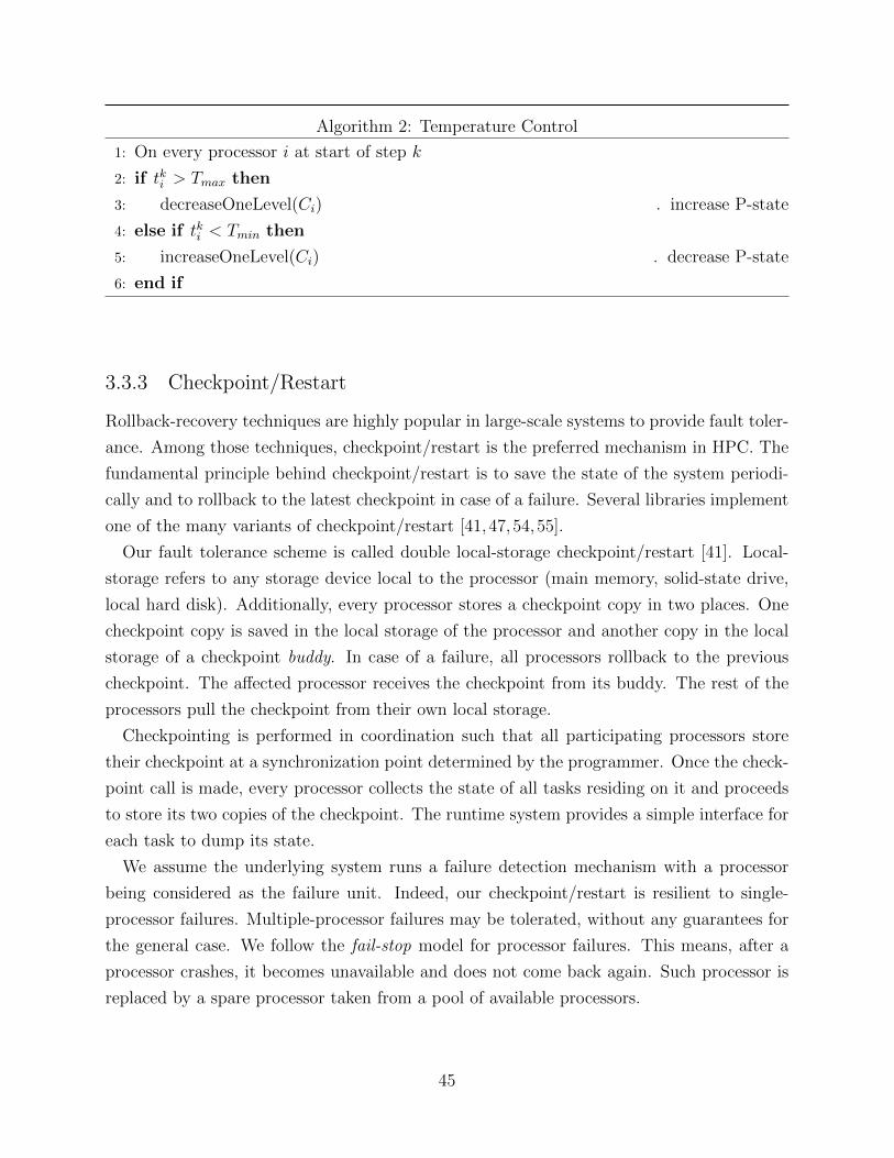
Algorithm 2: Temperature Control
1: On every processor i at start of step k
2: if tki > Tmax then
3: decreaseOneLevel(Ci) . increase P-state
4: else if tki < Tmin then
5: increaseOneLevel(Ci) . decrease P-state
6: end if
3.3.3 Checkpoint/Restart
Rollback-recovery techniques are highly popular in large-scale systems to provide fault toler-
ance. Among those techniques, checkpoint/restart is the preferred mechanism in HPC. The
fundamental principle behind checkpoint/restart is to save the state of the system periodi-
cally and to rollback to the latest checkpoint in case of a failure. Several libraries implement
one of the many variants of checkpoint/restart [41,47,54,55].
Our fault tolerance scheme is called double local-storage checkpoint/restart [41]. Local-
storage refers to any storage device local to the processor (main memory, solid-state drive,
local hard disk). Additionally, every processor stores a checkpoint copy in two places. One
checkpoint copy is saved in the local storage of the processor and another copy in the local
storage of a checkpoint buddy. In case of a failure, all processors rollback to the previous
checkpoint. The affected processor receives the checkpoint from its buddy. The rest of the
processors pull the checkpoint from their own local storage.
Checkpointing is performed in coordination such that all participating processors store
their checkpoint at a synchronization point determined by the programmer. Once the check-
point call is made, every processor collects the state of all tasks residing on it and proceeds
to store its two copies of the checkpoint. The runtime system provides a simple interface for
each task to dump its state.
We assume the underlying system runs a failure detection mechanism with a processor
being considered as the failure unit. Indeed, our checkpoint/restart is resilient to single-
processor failures. Multiple-processor failures may be tolerated, without any guarantees for
the general case. We follow the fail-stop model for processor failures. This means, after a
processor crashes, it becomes unavailable and does not come back again. Such processor is
replaced by a spare processor taken from a pool of available processors.
45

Algorithm 3: Communication Aware Load Balancing
1: On Master processor2: for i ∈ [1, n] do3: taskT icksk−1i = taskT imek−1i × fk−1
mk−1i
4: totalT icks += taskT icksk−1i
5: end for6: for i ∈ [1, p] do7: procT icksk−1i = procT imek−1i × fk−1i
8: freqSum += fki9: end for
10: createOverHeapAndUnderSet()11: while overHeap NOT NULL do12: donor = deleteMaxHeap(overHeap)13: if numForeignObjs(donor) > 0 then14: bestTask = getForeignTask(donor)15: else16: bestTask = getRandomTask(donor)17: end if18: sortedProcsList = getBestProcsList(bestTask)19: bestProc = getBestProc(sortedProcsList)20: mk
bestTask = bestProc21: procT icksk−1donor− = taskT icksk−1bestTask
22: procT icksk−1bestProc+ = taskT icksk−1bestTask
23: updateHeapAndSet()24: end while25:
26: procedure isHeavy(i)27: return procT icksk−1i > (1 + tolerance) ∗ totalT icks28: ∗(fki /freqSum)29:
30: procedure isLight(i)31: return procT icksk−1i < totalT icks ∗ fki /freqSum32:
33: procedure getBestProcList(bestTask)34: for i ∈ underSet do35: bestProcs[i].comm = getCommForTask(i,bestTask)36: bestProcs[i].procId = i37: end for38: return bestProcs39:
46

TimeFailure
Processor X
Processor Y
TC
& L
B
Chec
kpoin
t
Res
tartProcessor X'
Task A Task B Task D Task ETask C
Iteration i Iteration (i+1)Iteration (i-1)TC
& L
B
Chec
kpoin
t
TC
& L
B
...
...
...
...
Iteration (i+2) Iteration (i+2)
Figure 3.3: Dynamic power management and resilience framework.
3.3.4 Framework
In this section, we explain how we provide controllable resilience for HPC systems by bringing
together all three modules of our approach, i.e., temperature control (TC), communication
aware load balancing (LB) and checkpoint-restart. Figure 3.3 shows our framework with a
system of two processors (X and Y ) running a total of five tasks (from A to E) that are
executed in each iteration of a parallel program. The initial distribution of tasks places tasks
A and B on processor X while tasks C, D, and E are mapped to processor Y .
As Figure 3.3 shows, the program performs temperature control and load balancing (TC &
LB) several times during a checkpointing period, i.e., between two adjacent checkpoints. The
runtime system routinely adjusts the frequency of processors and solves the load imbalance
that may appear. This temperature-capping process decreases the failure rate. However, if
a failure occurs, the checkpoint/restart mechanism provides fault tolerance. The program
performs several iterations until the TC & LB modules are called after iteration i. The
TC module detects processor Y running at a temperature higher than the max threshold
and reduces its frequency. Following this, the LB module takes control and removes the
load imbalance by migrating task D from Y to X as outlined in Algorithm 3. The system
checkpoints after iteration i+ 1 and continues execution. A failure takes down processor X
during iteration i + 2, which gets replaced by a spare processor that we call processor X ′.
The checkpoint buddy of processor X provides checkpoint data for X to the replacement
processor X ′ to resume execution until the program finishes.
3.4 Experiments
In this section, we provide a comprehensive experimental evaluation of our techniques using
three different applications. The first one is Jacobi2D : a canonical benchmark that iteratively
applies a five-point stencil over a 2D grid of points. The second application, Wave2D, uses
a finite difference scheme over a 2D discretized grid to calculate the pressure resulting from
47

an initial set of perturbations. The third application, Lulesh, is a shock hydrodynamics
application that was defined and implemented by Lawrence Livermore National Laboratory
(LLNL) [56]. More details about these applications can be found in Appendix B.
The rest of this section describes our implementation, testbed and experimental results.
All experimental results are based on real hardware, and this section does not present any
simulation results.
3.4.1 Implementation Using Charm++
Charm++ is a parallel programming runtime system that leverages processor virtualization.
It provides a methodology where the programmer divides the program into smaller chunks
(objects or tasks) that are distributed among the p available processors by Charm++’s
adaptive runtime system [45]. Each of these small chunks is a migratable C++ object that
can reside on any processor. The runtime system tracks task execution time and maintains
this log in a database to be used by a load balancer for quantifying the amount of work in
each task [30].
Based on this information, if the load balancer in the runtime system detects load im-
balance, it migrates objects from an overloaded processor to an underloaded one. At small
scales, the cost of the entire load balancing process, from instrumentation through migration,
is generally a small portion of the total execution time, and less than the improvement that
it provides in execution time. When load balancing costs are significant, a strategy must
be chosen or adapted to match the application’s needs [31]. Our communication-aware load
balancer can be adapted to existing hierarchical schemes, which have been shown to scale
to the largest machines available [32]. More details about Charm++ load balancing can be
found in Chapter 2.
Charm++ implements a coordinated checkpointing strategy in which all processors coor-
dinate their checkpoints to form a consistent global state. Global state includes application-
specific data representing all object data as well as the runtime system state that constitutes
virtual processor data. Each physical processor keeps a copy of the runtime system state
with an arbitrary number of objects and their states. The Charm++ runtime keeps an
image of each object on two processors. The first copy resides on the processor which hosts
the object whereas the other copy is kept on the buddy processor. During checkpointing
each processor performs two concurrent steps: 1) packs its system state and sends it to its
buddy, 2) packs the user data representing all objects it hosts and sends it to its buddy. In
case of a crash, the recovery process is triggered in which all processors rollback to the most
48

Parameter Lulesh Jacobi2D Wave2D
δ (s) 9.57 7.65 8.01Tavg(
◦ C) 55.31 53.42 55.56M (s) 40.31 44.40 39.02τ(s) 18.2 18.4 17.0R (s) 2.2 1.52 1.60Recovery(%) 33.31 29.05 31.19Checkpointing(%) 21.40 20.11 20.89Restart(%) 5.38 3.48 4.03
Table 3.3: Application parameters for NC case
recent checkpoint. The crashing processor is either replaced by a new processor or its ob-
jects are distributed among existing processors. The object data for the crashing processor
is recovered from its buddy.
3.4.2 Testbed and Experimental Settings
We evaluated our scheme on the Energy Cluster described in Appendix A. This cluster uses
a Liebert power distribution unit installed on the rack containing the cluster to measure the
machine power at 1 second intervals on a per-node basis. We gather these readings for each
experiment and integrate them over the execution time to obtain the total machine energy
consumption.
In Section 3.2.1, we estimated the MTBF for our cluster (M) to be in the range of 24 - 55
days. To carry out experiments representative of a much larger system, we scale our cluster
M proportionally. We chose anm of 1 hour at 40◦ C per socket. For a system of 690K sockets,
these settings emulate an m of 10 years per socket. After demonstrating the accuracy of
our model by showing that it closely matches experimental results, we make predictions for
larger machines. The three applications that we considered exhibited different temperature
profiles. Therefore, to make our experiments realistic, we used actual temperature values
to estimate M for each application for experiments without temperature restraint. More
precisely, we estimate M using the maximum temperature that each of the 32 nodes reaches
for each application. Table 3.3 shows the cluster-wide average max temperatures for each
application in case of no temperature restraint. We refer to this baseline case as NC for the
rest of the chapter. For experiments where we restrain temperatures, we use the maximum
temperature threshold to estimate M . The values of M corresponding to each temperature
threshold are shown in Table 3.4. After determining M for each temperature threshold,
we generate sequences of exponential random numbers for each experiment, by taking each
49

44 46 48 50 52 540
2
4
6
8
10
12
14
16
Max allowed temperature (C)
Re
du
ctio
n in
exe
cu
tio
n t
ime
(%
)
2.14X
1.86X
1.62X1.42X
1.23X
1.07X
Model
Experiment
(a) Lulesh
44 46 48 50 52 540
2
4
6
8
10
12
14
16
Max allowed temperature (C)
Re
du
ctio
n in
exe
cu
tio
n t
ime
(%
)
2.21X
1.93X
1.68X
1.46X
1.28X
1.11X
Model
Experiment
(b) Wave2D
42 44 46 48 50 520
2
4
6
8
10
12
14
16
Max allowed temperature (C)
Re
du
ctio
n in
exe
cu
tio
n t
ime
(%
)
2.30X
2.00X 1.74X
1.52X
1.32X
1.15X
Model
Experiment
(c) Jacobi2D
Figure 3.4: Reduction in execution time for different temperature thresholds
M as the distribution mean. We manually insert faults according to these random number
sequences for each experiment, by killing a process on any one of the nodes using the kill
-9 command to wipe off all data. To recover from the artificially inserted failures, we
calculate the optimum checkpoint period (τ) for each experiment as follows [52]:
τ =√
2δM − δ (3.6)
Given that τ depends on M and the checkpoint time (δ), we obtain a different optimum
checkpoint period for each application when running at a given temperature threshold. The
δ for each application is listed in Table 3.3.
50

Tmax 54 52 50 48 46 44 42
M 43.8 50.4 57.8 66.4 76.2 87.5 100.2
Table 3.4: MTBF (sec) for different temperature thresholds (42◦ C - 54◦ C)
3.4.3 Experimental Results
To establish and to quantify the benefits of our scheme and to validate the accuracy of our
model (outlined in Section 5.4), we carried out a number of experiments. We demonstrate
how we can improve reliability using temperature control and compare the execution time for
experiments with and without temperature control. All experiments reported in this section
are compared to the baseline experiments (represented by NC) where all processors always
operate at the max frequency without any temperature control. Since the load balancing
technique is not the main focus of this chapter, we would not be giving a detailed comparison
of the improved load balancer proposed in Section 3.3 and the one proposed in Chapter 2.
However, our proposed new strategy does improve execution time for all three applications.
For Tmax =49◦ C, the communication-aware load-balancer can reduce execution time by
14%, 18%, and 5% for Wave2D, Lulesh and Jacobi2D, respectively, compared to the load-
balancer proposed in our earlier work [46]. Each data point (experiment) reported in this
section represents a benchmark running for more than 1 hour and being subject to at least
40 faults.
Table 3.3 lists the average maximum temperature for each application. Both Lulesh and
Wave2D have an average maximum temperature that is 2◦ C higher than that for Jacobi2D.
Due to this difference in temperature profile, we ran Jacobi2D for a maximum temperature
threshold range of 42◦ C-52◦ C as opposed to 44◦ C-54◦ C used for Lulesh and Wave2D. This
difference in thermal profile is also responsible for making different applications operate at
different average frequencies. For example, when running below a temperature threshold of
46◦ C, the average frequencies across the cluster for Lulesh, Jacobi2D and Wave2D, were
2.30 Ghz, 2.31GHz and 2.27 GHz, respectively. Although our testbed has a maximum
Turbo Boost frequency of 2.8Ghz, using DVFS to restrain temperatures resulted in lower
average frequency for all applications. A detailed discussion about the interaction between
temperature, frequency and performance can be found in Chapter 2.
Figure 3.4 shows percentage reduction in execution time using both temperature restraint
and load balancing compared to the baseline experiments, i.e., NC. The two curves in
each plot compare experimental results with model predictions. The model predictions for
Figure 3.4 were gathered by feeding checkpoint time, slowdown, restart time and useful
work time to Equation 3.5 and using golden section search and parabolic interpolation to
51

optimize τ for minimum total execution time. The inverted U shape of all three curves
strongly suggests a tradeoff between reliability (M) and the DVFS induced slowdown (µ)
due to temperature restraint. Figure 3.4 also shows the ratio of M for the machine using our
scheme relative to the NC case. For example, by restraining temperatures to 42◦ C in case
of Jacobi2D, M for the machine increased 2.3 times compared to the case of NC. Hence,
restraining the temperature to a lower value may decrease the benefits of our scheme but it
would always improve estimated reliability of the machine.
3.4.4 Interplay Between Temperature, MTBF and CheckpointingOverheads
MTBF for a machine (M) is dependent on each processor’s temperature. Higher processor
temperatures for Lulesh and Wave2D imply a lower M than Jacobi2D (Table 3.3). This
forces Wave2D and Lulesh to spend a higher percentage of time in recovery as they en-
counter more failures compared to Jacobi2D (Table 3.3). Although M for Wave2D and
Lulesh are close in the case of NC, they spend different percentages of time in recovery,
i.e., 31.19% and 33.31% respectively. This observation can be explained by looking at their
τ values (Table 3.3). According to Equation 3.6, a larger checkpoint time (δ in Table 3.3)
for Lulesh results in a larger τ which increases the average recovery time for Lulesh ( τ+δ2
in Equation 3.5). On the other hand, Lulesh’s higher τ causes it to spend almost an equal
percentage of time in checkpointing as Jacobi2D and Wave2D , i.e., 21.40% (Table 3.3),
despite Lulesh’s large δ. Although the time per checkpoint (δ) for Lulesh is the highest,
the product of the number of checkpoints and δ is equal to other applications due to fewer
checkpoints(Wµτ− 1)
for Lulesh. Lulesh also spends 5.38% of its total time in restarts,
which can be attributed to the higher restart cost of 2.2 seconds (Table 3.3).
3.4.5 Comparing the Benefits Across Applications
Although all three applications have a inverted U shaped curve, their maxima occur at differ-
ent temperature thresholds. We define this optimum point for each application by the tuple
(Tmax, rmax), where Tmax is the temperature threshold corresponding to the point that rep-
resents the maximum reduction in execution time for an application. Figure 3.4 shows that
the optimum points for Jacobi2D, Wave2D, and Lulesh are (46◦ C,14.2%), (48◦ C,13.5%),
and (50◦ C,11%) respectively. We notice that the applications differ in both members of the
tuple. An application’s optimum point depends on the tradeoff between percentage reduc-
52

42 44 46 48 50 52 540
5
10
15
20
25
30
35
Max allowed temperature ( °C)
Execution tim
e p
enalty (
%)
Lulesh
Wave2D
Jacobi2D
Figure 3.5: Execution time penalty for DVFS
tion in each category of total time (recovery, checkpoint and restarting times), which is a
result of improvement in M , and its associated cost. This slowdown, including overhead
of object migration during load balancing, is shown in Figure 3.5. The slowdown for each
application increases as the temperature threshold decreases. As the temperature threshold
decreases, the frequency at which a processor could operate also decreases. The reduced
frequency in turn implies a higher slowdown. The slowdown is worse in case of CPU inten-
sive applications. Figure 3.5 points to a similar trend. Lulesh is the most CPU intensive
application whereas Jacobi2D has the highest memory foot print. Hence, the slowdown for
Lulesh is higher than Jacobi2D for all temperature thresholds. In general, we should expect
applications having high memory footprint to have smaller slowdown and hence, higher ben-
efits for using our scheme. Figure 3.4 shows that Jacobi2D has the most gain, i.e., 14.2%
using our scheme, whereas the gain for Lulesh is 11%. These gains validate our claim: lower
the slowdown, higher the gain for using our scheme.
Another observation that we can make is that the temperature threshold and the cost of
temperature control µ are directly related. Figure 3.5 shows that Lulesh had the maximum
slowdown leading to a larger optimum temperature threshold (50◦ C) and therefore it receives
the least reduction in execution time (11%) among all three applications. On the other
hand, Jacobi2D, experiences the least slowdown, which results in the highest reduction in
execution time, i.e., 14.2%, and the lowest optimum temperature threshold. The slowdown
for Wave2D lies in between Lulesh and Jacobi2D, which results in a reduction in execution
time that is between 11%-14.2%, i.e., 13.5%.
53

44 46 48 50 520
2
4
6
8
10
12
14
16
18
20
Maximum temperature threshold (C)
Reduct
ion/ In
crease
in e
ach
cate
gory
of tim
e (
%)
Recovery Checkpoint Restart Cost
L J L J 44
Maximum temperature threshold (°C)
L J L J 46
L J L J 48
L J L J 50
L J L J 52
L- Lulesh J - Jacobi2D
Figure 3.6: Gains/cost of increasing reliability for different temperature thresholds
3.4.6 Understanding Application Response to Temperature Restraint
All applications that we considered respond differently to temperature restraints which is
why each one has a different optimum point. For more insights, we compare and contrast
how Jacobi2D and Lulesh respond to temperature control in Figure 3.6. Here, we plot
the percentage of time reduced for each category of execution time (including recovery,
checkpoint, and restart times), as a percentage of total time taken in case of NC.
We used the following formula to determine the recovery percentage (preci ) corresponding
to the maximum temperature threshold of i◦ C for Figure 3.6:
preci =trecNC − treciTNC
∗ 100 (3.7)
where TNC is the total execution time in case of NC, trecNC is the recovery time for NC and treci
is the recovery time for the experiment where the maximum threshold was i◦ C. Figure 3.6
also shows the cost of temperature control for Lulesh and Jacobi2D which represents DVFS-
incurred slowdown in doing useful work (Wµ in Equation 3.5). This cost pcosti as well as the
percentage reduction in checkpoint pckpti and restart times presi are calculated similar to preci
in Equation 3.7. We make two observations from Figure 3.6.
First, we look at the total gain (sum of recovery, checkpointing and restart gains). While
the total gains are always greater for Lulesh compared to Jacobi2D (except for 44◦ C ), its
cost of temperature control is always significantly lesser than that for Lulesh. Hence, the
54

net gain (total gains - cost) for Jacobi2D makes it much more appropriate for our scheme
compared to Lulesh.
Next, we observe that prec48 , prec50 and prec52 are higher for Lulesh compared to Jacobi2D
whereas for lower thresholds, prec44 and prec46 are lower for Lulesh. Recall from Figure 3.4 that
Lulesh improves reliability of the system more than Jacobi2D, i.e., (1.86X, 2.14X) compared
to (1.74X, 2.00X) for thresholds of 46◦ C and 44◦ C, respectively. Even then, the high timing
penalty for Lulesh depicted in Figure 3.6 is limiting the gains from increased reliability. The
timing penalty not only contributes directly as cost of improving reliability by prolonging
useful work, it also indirectly affects the benefits of our scheme by limiting the gains that
we obtain in recovery. So if a timing penalty of µ gets added to the total execution time,
then the faults, checkpoints and restart that happen during µ essentially work to cancel out
some of the gains achieved by temperature restraint during the earlier part of execution.
The timing penalty is precisely what shrinks the gain bars in Figure 3.6. However, even
with the higher timing penalty of Lulesh, its gains are sufficient to reduce execution time as
compared to the case of NC.
3.4.7 Reduction in Energy Consumption
After highlighting how our scheme successfully reduces execution time and increases M ,
we now analyze the reduction in machine energy consumption that happens as a direct
consequence of our scheme. Figure 3.7 shows the percentage reduction in machine energy
consumption for each application compared to the baseline case (NC). These numbers
represent actual machine energy consumption for experiments measured using power meters.
The figure shows that we were able to reduce machine energy consumption by as much as
25% in case of Jacobi2D by restraining processor temperatures at 42◦ C. Although the
reduction in execution time contributes to reduction in energy consumption, the major part
of savings comes from temperature control which reduces the machine’s power consumption.
In addition to the reported reduction in machine energy, our scheme should also reduce the
cooling energy significantly (Chapter 2).
3.5 Projections
In Section 3.4, we thoroughly investigated our approach and validated our model by carefully
comparing it against experimental results. Now, we use the validated model to project the
benefits of our scheme for larger machines. We estimate improvement in machine efficiency
55
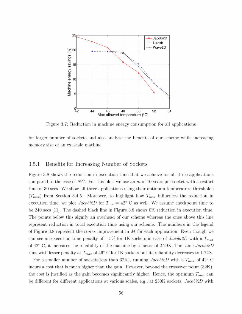
42 44 46 48 50 52 540
5
10
15
20
25
Max allowed temperature (°C)
Ma
ch
ine
en
erg
y s
avin
gs (
%)
Jacobi2D
Lulesh
Wave2D
Figure 3.7: Reduction in machine energy consumption for all applications
for larger number of sockets and also analyze the benefits of our scheme while increasing
memory size of an exascale machine.
3.5.1 Benefits for Increasing Number of Sockets
Figure 3.8 shows the reduction in execution time that we achieve for all three applications
compared to the case of NC. For this plot, we use an m of 10 years per socket with a restart
time of 30 secs. We show all three applications using their optimum temperature thresholds
(Tmax) from Section 3.4.5. Moreover, to highlight how Tmax influences the reduction in
execution time, we plot Jacobi2D for Tmax= 42◦ C as well. We assume checkpoint time to
be 240 secs [11]. The dashed black line in Figure 3.8 shows 0% reduction in execution time.
The points below this signify an overhead of our scheme whereas the ones above this line
represent reduction in total execution time using our scheme. The numbers in the legend
of Figure 3.8 represent the times improvement in M for each application. Even though we
can see an execution time penalty of 15% for 1K sockets in case of Jacobi2D with a Tmax
of 42◦ C, it increases the reliability of the machine by a factor of 2.29X. The same Jacobi2D
runs with lesser penalty at Tmax of 46◦ C for 1K sockets but its reliability decreases to 1.74X.
For a smaller number of sockets(less than 32K), running Jacobi2D with a Tmax of 42◦ C
incurs a cost that is much higher than the gain. However, beyond the crossover point (32K),
the cost is justified as the gain becomes significantly higher. Hence, the optimum Tmax can
be different for different applications at various scales, e.g., at 230K sockets, Jacobi2D with
56

1K 2K 4K 8K 16K 32K 64K 128K 256K−20
−10
0
10
20
30
40
Number of sockets
Re
du
ctio
n in
exe
cu
tio
n t
ime
(%
)
Jacobi2D (46 °C)−1.74X
Wave2D (48 °C)−1.73X
Lulesh (50 °C)−1.48X
Jacobi2D (42 °C)−2.29X
Figure 3.8: Execution time reduction for all applications at large scale
a Tmax of 42◦ C reduces the execution time by 38% compared to 32% if run at Tmax of 46◦ C.
Efficiency can be defined as the fraction of the total execution time, including the fault
tolerance overheads, that is spent in doing useful work. A decrease in total execution time
can be thought of as an improvement in machine efficiency. Figure 3.9 plots the machine
efficiency for Wave2D at Tmax = 48◦ C using the same parameters as Figure 3.8. Even
though we account for DVFS incurred slowdown in our efficiency calculation, our scheme
still improves machine efficiency significantly for larger socket counts. The numbers shown
in Figure 3.9 represent the ratio of efficiency for our scheme relative to the case of NC.
For less than 32K sockets, we get a lower efficiency compared to the case of NC (efficiency
< 1X). However, after 32K sockets, our scheme starts outperforming the NC case (> 1
efficiency values). For 340K sockets, our scheme is projected to operate the machine with
an efficiency of 0.22 (95% reduction in execution time) compared to 0.01 for the NC case.
Finally, for 350K sockets, the efficiency for NC case drops to 0.003 making the machine
almost non-operational using only checkpoint/restart, whereas our scheme can still operate
the machine at an efficiency of 0.20.
3.5.2 Sensitivity to Memory-per-socket and MTBF
The checkpoint time of 240 sec predicted in Kogge’s report [11] is made under the assump-
tion that an exascale machine will have 224K sockets with 64GB of memory per socket.
Adding more memory to the proposed machine increases the number of components that
57

1K 2K 4K 8K 16K 32K 64K 128K 256K 512K0
0.1
0.2
0.3
0.4
0.5
0.6
0.7
0.8
0.9
1
Number of sockets
Ma
ch
ine
Utiliza
tio
n
0.93X0.94X
0.95X
0.96X
0.99X
1.03X
1.10X
1.25X
1.50X
20.14X
Tmax
: 48 °C
NC
Figure 3.9: Projected efficiency for Wave2D
can significantly decrease the reliability. With the proposed memory size (13.6 PB), the
machine will have a flop-memory ratio of 0.01 Petaflops/TB which is far smaller than 96
Petaflops/TB and 134 Petaflops/TB for Sequoia and the K computer [13] respectively. To
evaluate if our scheme can enable an exascale system to have more memory, we predicted the
improvement in M as well as the reduction in execution time that our scheme can achieve
compared to the case of NC as we keep on increasing memory per socket. Adding memory
implies more data to checkpoint. We use the same methodology used in Kogge’s report [11]
to calculate the checkpoint time as we keep on increasing memory per socket. Figure 3.10
shows the results from our model for Jacobi2D projected on an exascale machine. MTBF
per socket can have a significant effect on the total execution time of an application. The
MTBF of LANL’s clusters is 10 years per socket [57] whereas Jaguar had a 50 years MTBF
per socket [58]. Other studies show MTBF per socket to be between 20-30 years [59, 60].
For capturing the sensitivity of our scheme to MTBF, we plotted lines corresponding to 5
different MTBF per socket ranging from 10-50 years. Figure 3.10 shows that our scheme
will decrease the execution time for any memory size per socket using any of the five MTBF
values. Even the two memory sizes used in Kogge’s report [11], i.e., 16GB and 64GB, will
end up benefitting from our scheme.
58

16 32 64 128 256−5
0
5
10
15
20
25
30
35
40
Mem per chip (GB)
Re
du
ctio
n in
exe
cu
tio
n t
ime
(%
)
10y
20y
30y
40y
50y
Figure 3.10: Reduction in execution time for different memory sizes of anexascale machine
59

CHAPTER 4Optimizing Performance Under a Power
Budget
The first part of the thesis emphasized the importance of thermal restraint for an HPC
data center. Chapter 2 presented empirical results showing significant reductions in energy
consumption of a 128-core cluster. Chapter 3 combined checkpointing and thermal restraint
to improve application performance. In the next two chapters, we aim to deal with another
important challenge that the HPC community faces: improving application performance
under a strict power constraint.
Applications do not yield a proportional improvement in performance as the processor
frequency is increased [61]. This insensitivity is mainly because memory accesses are much
slower compared to processor frequency. Memory accesses therefore introduce stalls in pro-
cessor cycles. The extent of improvement in application performance resulting from increased
processor frequency depends on the application’s computational and memory demands. As
we approach the exascale era, the thrust is more on power consumption than on energy
minimization. A strict power constraint poses a hard research challenge. DOE has currently
set a bound of 20MW for an exascale system, therefore available power must be used effi-
ciently to achieve the exascale goal. Scaling frequency via DVFS does not guarantee a strict
limit on the power consumption of a processor. However, the recently released Intel’s Sandy
Bridge family of processors provide an enticing option of limiting the power consumption
of a processor chip and memory (also available in IBM Power6 [62], Power7 [63] and AMD
Bulldozer [64] architectures). The power consumption for package and memory subsystems
can be user-controlled through the RAPL (Running Average Power Limit) library [65].
In this part of the thesis (Chapter 4 and Chapter 5), we use Intel’s power gov [66] library
that in turn uses RAPL to cap power of memory and package subsystems in order to optimize
60

application performance under a strict power budget for an overprovisioned system. An
overprovisioned system [14] has more nodes than a conventional system operating under
the same power budget. It cannot simultaneously power all nodes at peak power. However,
capping package (CPU) and memory power below peak power can enable an overprovisioned
system to operate all nodes simultaneously. Under a strict power budget, running the
application on fewer nodes with a higher CPU/memory power per-node can sometimes be
less efficient than running it on more nodes with relatively lower power per node. Capping
the CPU and memory power to lower values enables us to utilize more nodes for executing
an application. However, each additional node utilized has a fixed cost of powering up the
motherboard, power supply, fans and disks referred to as the base power. The base power of
a node determines the ease with which additional nodes can be utilized in an overprovisioned
system. The opportunity cost of base power for these additional nodes is the performance
benefit that can be achieved by increasing the CPU and memory power for the existing set
of nodes. This opportunity cost can vary between applications.
The work presented in this chapter optimizes the number of nodes and the subsequent
distribution of power between CPU and memory for an application under a strict power
budget. The major contributions of this chapter are listed below:
• We propose an interpolation scheme that captures the effects of strong scaling an
application under different CPU and memory power distributions with minimal profile
information.
• We present experimental results showing speedups of up to 2.2X using an overprovi-
sioned system compared to the case where CPU and memory powers are not capped.
• We show the optimized CPU and memory power distributions for different applications
and examine the factors that influence them.
• We analyze the effect and importance of base power on achievable speedup for an
overprovisioned system.
The rest of the chapter is organized as follows. Section 4.1 describes related work. In
Section 4.2, we outline our interpolation scheme. Section 4.3 details our experimental setup.
Section 4.4 presents a case study that demonstrates the working details of our scheme. In
Section 4.5 we present our experimental results.
61

4.1 Related Work
To the best of our knowledge, this chapter provides the first study that estimates and
analyzes the optimized distribution of power among the CPU and the memory subsystem,
in the context of an overprovisioned system under a strict power budget. Rountree et al [65]
have studied the variation in application performance under varying power bounds using
RAPL. In continuation of this work, Patki et al [14] proposed the idea of overprovisioning
the compute nodes in power-constrained high performance computing. Their work relies
on selecting the best configuration out of a set of profiled configurations. Because of the
sheer number of possible configurations, exhaustively profiling an application for all possible
node counts, CPU power caps and memory power caps is practically infeasible. Our work
introduces a novel interpolation scheme, that takes into account the effects of strong scaling
an application under different CPU and memory power caps and estimates the missing
configurations. Our work also differs from prior work [14] since we take into account the
effect of memory capping that can significantly improve the speedups for most applications.
Another novel aspect is that our scheme is based on total machine power which includes
base power, i.e., power consumption of everything other than the CPU and the memory
subsystem, that can significantly alter the observed speedups across applications.
The idea of overprovisioning has been studied and implemented in the architecture com-
munity in a similar context [67] e.g. Intel’s Nehalem has overprovisioned cores. The CPU
can either run all of these cores at lower clock frequencies or a few of them at highest clock
frequencies due to power and thermal bounds. Additionally, earlier work has mostly focussed
on reducing energy consumption under a time bound for HPC applications. Rountree et al [2]
have used linear programming to reduce energy consumption with negligible execution time
penalty. In our earlier work, we have used DVFS to trade execution time for lower cooling
and machine energy consumptions [33,46].
4.2 Approach
Power consumption of different applications varies significantly. Moreover, the usefulness
of increasing the power budget of an application also varies between applications [61]. We
formulate our problem statement as follows:
Optimize the numbers of nodes (n), the CPU power level (pc) and memory power level
(pm) that minimizes execution time (t) of an application under a strict power budget (P ),
on an overprovisioned high performance computation cluster with pb as the base power per
62

Variable Description
W Wattspb node base power (W)pc CPU/Package power cap (W)pm memory power cap (W)Pc set of allowed CPU caps usedPm set of allowed memory caps usedN set of number of nodes usedPc set of CPU power caps used for profiling in Step 1Pm set of memory power caps used for profiling in Step 1N set of number of nodes used for profiling in Step 1P maximum allowed power budget (W)t execution time for an application (s)
Table 4.1: Terminology
node.
In this section, we outline our interpolation scheme that estimates execution time using
application profiles for different scales, CPU power levels and memory power levels. The ter-
minology used in the chapter is defined in Table 4.1. We denote an operating configuration by
(n×pc, pm) where n is the number of nodes and pc, pm are the CPU and memory power caps,
respectively. To determine the optimized configuration for running an application, we need
to profile the application for each configuration (n× pc, pm) where n ∈ N , pc ∈ Pc, pm ∈ Pm.
Such exhaustive profiling adds up to a total of |N | × |Pc| × |Pm| possible configurations,
assuming Pc and Pm have integral values only. Such exhaustive profiling of an application is
practically infeasible because of the sheer number of possible configurations. For example,
in a cluster with only 20 nodes, 71 CPU power levels and 28 memory power levels, we would
need to profile the application for 39, 760 possible configurations, which is practically infea-
sible. Therefore, we break the application performance analysis into two steps: performance
measurement by actual profiling (Step 1) followed by performance estimation using curve
fitting/ interpolation (Step 2).
Step 1: Performance measurement by actual profiling
We start application profiling by running it for a selected set of configurations that span the
entire range of available configurations. In other words, we only profile the application for a
subset of the total possible configurations, i.e., (n× pc, pm) where n ∈ N , pc ∈ Pc, pm ∈ Pm.
63

Step 2: Performance prediction by curve fitting or interpolation
In this step, we use curve fitting on the profiled data obtained in Step 1 to estimate the
execution time for any possible configuration (n×pc, pm) where n ∈ N , pc ∈ Pc and pm ∈ Pm.
Behavior of execution time (t) with n, pc, and pm, can be represented in a 4D plot. However,
visualizing a 4D plot can be tedious. Hence, we present application profiles by plotting t
against the total power p in 2D, where p takes pc, pm, and n into account, using the following
equation:
p = n ∗ (pb + pc + pm) (4.1)
Presenting the profile in a 2D plot facilitates its visualization and makes it easier to determine
the optimized configuration. To estimate execution time for any configuration we need to
find the relationship of execution time to power consumption across the three dimensions,
i.e., n, pc, and pm. Beginning with the |N | × |Pc| × |Pm| actually profiled configurations in
Step 1, interpolation is accomplished in the following three steps:
1. Interpolation across memory power: For each pair of (n, pc) where n ∈ N , pc ∈ Pc, we
fit a curve φn,pc(x) across the profiled values of memory caps, i.e., pm ∈ Pm, where
x ∈ Pm. This process yields |N | × |Pc| such curves. A given curve, φn,pc , can be used
to obtain an estimate of t corresponding to any pm ∈ Pm using n nodes capped at CPU
power level of pc. Using the φn,pc curves, we can estimate the execution times for all
configurations (n× pc, pm) where n ∈ N , pc ∈ Pc, and pm ∈ Pm.
2. Interpolation across node counts: To capture the behavior of strong scaling, we fit a
curve ψpc,pm(x) across the profiled values of n, i.e., n ∈ N , where x ∈ N , for each
pair of (pc, pm) where pc ∈ Pc and pm ∈ Pm. This process results in |Pc| × |Pm| strong
scaling curves. A given strong scaling curve, ψpc,pm , can estimate t for any n ∈ N where
each node is operating under CPU and memory power caps of pc and pm respectively.
These strong scaling curves can be used to obtain values of t for all configurations
(n× pc, pm) where n ∈ N, pc ∈ Pc, and pm ∈ Pm.
3. Interpolation across CPU power: Finally, we interpolate t across CPU power. We fit
a curve θn,pm(x) across the profiled values of pc (pc ∈ Pc) where x ∈ Pc, for every
pair of (n, pm) such that n ∈ N and pm ∈ Pm. We retrieve |N | × |Pm| curves for
interpolating across pc. A given curve, θn,pm , estimates t for any pc ∈ Pc using n nodes
operating under a memory power cap of pm. These θn,pm curves can be used to estimate
64

execution times for all possible configurations, i.e., (n× pc, pm), where n ∈ N , pc ∈ Pcand pm ∈ Pm.
4.3 Setup
We used the Power Cluster to carry out all experiments for this chapter (see Appendix A).
The Intel Sandy Bridge processor family supports on board power measurement and capping
through the Running Average Power Limit (RAPL) interface [36]. The Sandy Bridge archi-
tecture has four power planes: Package (PKG), Power Plane 0 (PP0), Power Plane 1 (PP1)
and DRAM. RAPL is implemented using a series of Machine Specifics Registers (MSRs) that
can be accessed to read power readings for each power plane. RAPL supports power capping
PKG, PP0 and DRAM power planes by writing into the relevant MSRs. The average base
power per node (pb) for our cluster was 38 watts. The base power was measured using the
in-built power meters on the Power Distribution Unit (PDU) that powers our cluster. We
experimented with Lulesh, Wave2D and LeanMD to demonstrate the use of our scheme (see
Appendix B).
4.4 Case Study: Lulesh
In this section, we demonstrate the application of our scheme in estimating the optimized
configuration for an iterative application under a strict power budget by considering the
Lulesh application. The profiling experiments were conducted on the Power cluster outlined
in Appendix A. The following CPU and memory power caps were selected for profiling (Step
1 ):
Pc = {28, 32, 36, 44, 50, 55}
Pm = {8, 10, 14, 18}
Since determining the optimized number of nodes (n) is part of our scheme, we profile the
application for strong scaling as well:
N = {5, 8, 12, 16, 20}
Figure 4.1 shows Lulesh’s execution profile for some of these configurations. The Y-axis
corresponds to the average execution time per step, and the X-axis shows the total power
65

0 400 800 1200 1600 2000 2400
4
8
12
16
20
Total power (W)
Exe
cu
tio
n t
ime
(se
cs)
(5 x pc ,8)
(5 x pc ,18)
(12 x pc ,8)
(12 x pc ,10)
(12 x pc ,18)
(20 x pc ,8)
(20 x pc ,10)
(20 x pc ,18)
Figure 4.1: Average time per step of Lulesh for configurations selected in Step 1
(p) of the system (calculated using Equation 4.1). Each set of configurations in Figure 4.1
contains 6 points corresponding to varying CPU power, i.e., pc ∈ {28, 32, 36, 44, 50, 55}.The leftmost point for each set corresponds to pc = 28W, whereas the rightmost point uses
pc=55W. Based on the profile data, we can pick an efficient configuration for a given power
budget as follows: We draw a vertical line at the given power budget P and choose the
lowest point on or to the left of that vertical line. Following are three examples of finding
the optimized configurations for a given power budget (P ).
• P = 1200W: the best profiled configuration is (12× 44, 18).
• P = 1600W: the best profiled configuration is (20 × 32, 10). In this case, using more
nodes with each node capped at relatively lower CPU and memory power levels is
better compared to the P = 1200W case, in which fewer nodes are used at a higher
CPU and memory power levels.
• P = 800W: Since we do not have profile data close to the power budget of 800W,
we have to proceed leftwards to the (5 × 55, 18) configuration. This configuration
corresponds to a total power consumption of 555W. Hence, the available power is not
completely used which makes it an inferior solution.
66
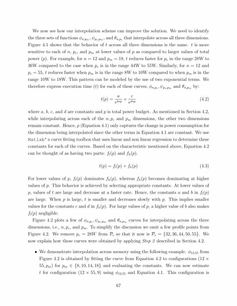
We now see how our interpolation scheme can improve the solution. We need to identify
the three sets of functions φn,pm , ψpc,pm , and θn,pc that interpolate across all three dimensions.
Figure 4.1 shows that the behavior of t across all three dimensions is the same. t is more
sensitive to each of n, pc, and pm at lower values of p as compared to larger values of total
power (p). For example, for n = 12 and pm = 18, t reduces faster for pc in the range 28W to
36W compared to the case when pc is in the range 44W to 55W. Similarly, for n = 12 and
pc = 55, t reduces faster when pm is in the range 8W to 10W compared to when pm is in the
range 10W to 18W. This pattern can be modeled by the use of two exponential terms. We
therefore express execution time (t) for each of these curves, φn,pc , ψpc,pm and θn,pm by:
t(p) =a
eb∗p+
c
ed∗p(4.2)
where a, b, c, and d are constants and p is total power budget. As mentioned in Section 4.2,
while interpolating across each of the n, pc and pm dimensions, the other two dimensions
remain constant. Hence, p (Equation 4.1) only captures the change in power consumption for
the dimension being interpolated since the other terms in Equation 4.1 are constant. We use
Matlab’s curve fitting toolbox that uses linear and non linear regression to determine these
constants for each of the curves. Based on the characteristic mentioned above, Equation 4.2
can be thought of as having two parts: fl(p) and fh(p).
t(p) = fl(p) + fh(p) (4.3)
For lower values of p, fl(p) dominates fh(p), whereas fh(p) becomes dominating at higher
values of p. This behavior is achieved by selecting appropriate constants. At lower values of
p, values of t are large and decrease at a faster rate. Hence, the constants a and b in fl(p)
are large. When p is large, t is smaller and decreases slowly with p. This implies smaller
values for the constants c and d in fh(p). For large values of p, a higher value of b also makes
fl(p) negligible.
Figure 4.2 plots a few of φn,pc , ψpc,pm and θn,pm curves for interpolating across the three
dimensions, i.e., n, pc, and pm. To simplify the discussion we omit a few profile points from
Figure 4.2. We remove pc = 28W from Pc so that it now is Pc = {32, 36, 44, 50, 55}. We
now explain how these curves were obtained by applying Step 2 described in Section 4.2.
• We demonstrate interpolation across memory using the following example. φ12,55 from
Figure 4.2 is obtained by fitting the curve from Equation 4.2 to configurations (12 ×55, pm) for pm ∈ {8, 10, 14, 18} and evaluating the constants. We can now estimate
t for configuration (12 × 55, 9) using φ12,55 and Equation 4.1. This configuration is
67
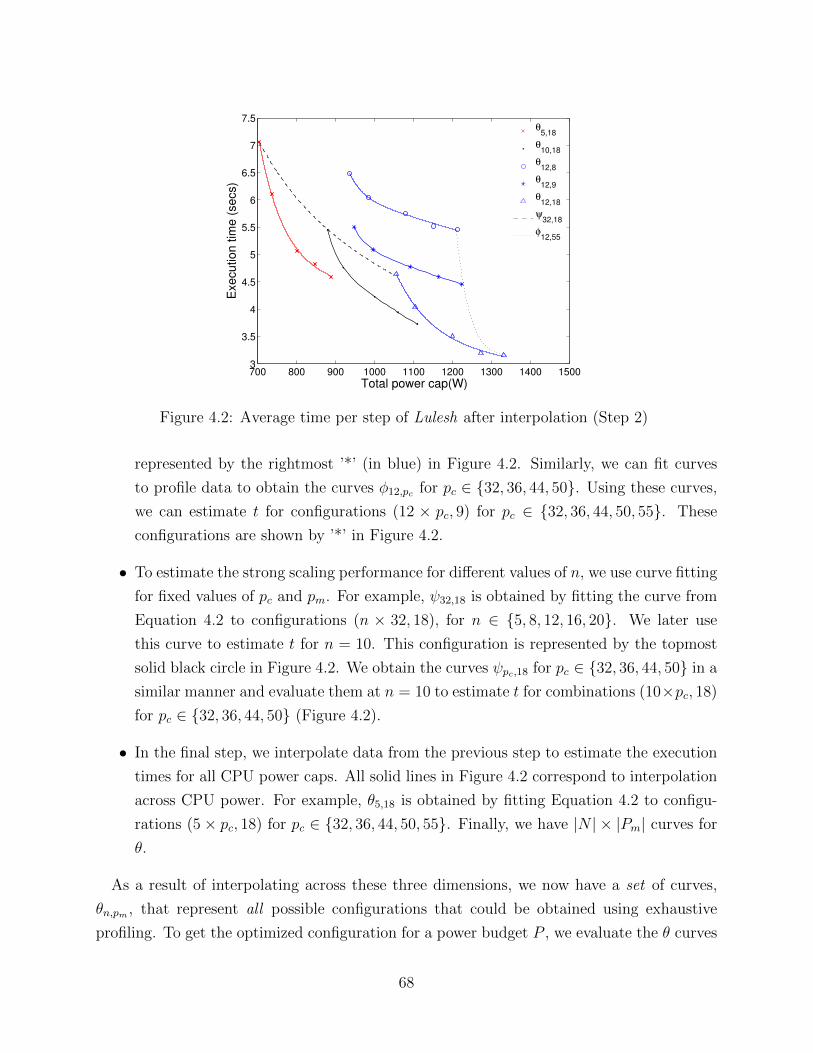
700 800 900 1000 1100 1200 1300 1400 15003
3.5
4
4.5
5
5.5
6
6.5
7
7.5
Total power cap(W)
Exe
cu
tio
n t
ime
(se
cs)
θ5,18
θ10,18
θ12,8
θ12,9
θ12,18
ψ32,18
φ12,55
Figure 4.2: Average time per step of Lulesh after interpolation (Step 2)
represented by the rightmost ’*’ (in blue) in Figure 4.2. Similarly, we can fit curves
to profile data to obtain the curves φ12,pc for pc ∈ {32, 36, 44, 50}. Using these curves,
we can estimate t for configurations (12 × pc, 9) for pc ∈ {32, 36, 44, 50, 55}. These
configurations are shown by ’*’ in Figure 4.2.
• To estimate the strong scaling performance for different values of n, we use curve fitting
for fixed values of pc and pm. For example, ψ32,18 is obtained by fitting the curve from
Equation 4.2 to configurations (n × 32, 18), for n ∈ {5, 8, 12, 16, 20}. We later use
this curve to estimate t for n = 10. This configuration is represented by the topmost
solid black circle in Figure 4.2. We obtain the curves ψpc,18 for pc ∈ {32, 36, 44, 50} in a
similar manner and evaluate them at n = 10 to estimate t for combinations (10×pc, 18)
for pc ∈ {32, 36, 44, 50} (Figure 4.2).
• In the final step, we interpolate data from the previous step to estimate the execution
times for all CPU power caps. All solid lines in Figure 4.2 correspond to interpolation
across CPU power. For example, θ5,18 is obtained by fitting Equation 4.2 to configu-
rations (5× pc, 18) for pc ∈ {32, 36, 44, 50, 55}. Finally, we have |N | × |Pm| curves for
θ.
As a result of interpolating across these three dimensions, we now have a set of curves,
θn,pm , that represent all possible configurations that could be obtained using exhaustive
profiling. To get the optimized configuration for a power budget P , we evaluate the θ curves
68

800 1000 1200 1400 1600 1800 20001
1.2
1.4
1.6
1.8
2
2.2
Total power budget (W)
Sp
ee
du
p
Interp. ObservedInterp. EstimateProfiling
(a) Lulesh
800 1000 1200 1400 1600 1800 20001
1.2
1.4
1.6
1.8
2
2.2
Total power budget (W)
Sp
ee
du
p
Interp. ObservedInterp. EstimateProfiling
(b) Wave2D
800 1000 1200 1400 1600 1800 20001
1.2
1.4
1.6
1.8
2
2.2
Total power budget (W)
Sp
ee
du
p
Exhaustive ProfilingInterp. ObservedInterp. EstimateProfiling
(c) LeanMD
Figure 4.3: Speedups obtained using CPU and memory power capping in an over-provisioned system
for that P and chose the configuration that results in the minimum t. If the curve θn0,p0m(P )
results in the minimum t = t0 , the optimized configuration is given by (n0× Pn0−pb−p0m, p0m)
after using Equation 4.1 and solving for pc.
4.5 Results
In this section, we use our interpolation model to estimate optimized configurations for
different power budgets for the three parallel applications mentioned in Section 4.3. Machine
vendors specify the thermal design power (TDP) for CPU and memory subsystems. These
69

numbers represent the maximum power each of these subsystems can draw while operating
within the thermal limits. Data centers do not take application characteristics into account
and therefore calculate the total power assuming that each node can draw the TDP wattage
specified by the manufacturer. We refer to this configuration as the baseline configuration .
The baseline configuration for a power budget of P is given by:
(nb × TDPc, TDPm)
where nb =
⌊P
pb + TDPc + TDPm
⌋,
and TDPc and TDPm represent the CPU and memory TDP values respectively. For our
testbed cluster, TDPc = 95W and TDPm = 35W. TDP of a node for our cluster totals
to 168W after adding the base power of 38W. Hence, for the baseline case we employ the
maximum number of nodes, without power capping, accounting for a maximum possible
power draw of up to 168W per node, i.e., nb = P168
. We compare the benefits resulting from
power capping CPU and memory subsystems using our scheme against the baseline case for
different power budgets. We use speedup over the baseline case as the metric for comparison.
Speedup is defined as the ratio of the execution time for the baseline case and the execution
time that results from the optimized configuration estimated by our scheme. We perform
real experiments to corroborate the estimates made using our scheme. In particular, we
present results to gauge the effectiveness of our approach to meet the following criterion:
• Speedup achieved: Comparing the best configurations from profiled data (Step 1) to
the best configurations estimated using our scheme (Step 2).
• Quality of solution: Comparing model estimates to actual experimental results
• Cost of estimating the optimized configuration: Amount of profiling required to make
accurate predictions.
4.5.1 Benefits of Using our Interpolation Scheme
In Figure 4.3, we present the speedups achieved using power capping in an over-provisioned
system for different power budgets. The ‘Profiling’ curve plots the actual speedups that
are obtained by selecting the optimized configuration from the profiled data from Step 1
(without interpolation). The ’Interp. Estimate’ plots the estimated speedups obtained from
the interpolated curves from Step 2. We do actual experiments for the optimal configurations
predicted in Step 2 and plot the observed speedups shown as the ‘Interp. Observed’ curve.
70

We can see from Figure 4.3 that the observed speedups (’Interp. Observed’) match closely to
the estimated speedups (’Interp. Estimate’). The difference in the estimated and observed
speedups can be attributed to system/cluster noise and to the estimation accuracy of our
interpolation scheme. Speedups of Lulesh, Wave2D, LeanMD fall in the range [1.55,1.80],
[1.45,1.9], [1.57,2.2] respectively. Although each application ends up in a different speedup
range, we get a minimum speedup of at least 1.45X for any power budget. Speedup that an
application can achieve is attributed to two factors:
• The difference between the CPU/memory TDP and the actual (measured) power con-
sumed by the CPU/memory.
• The sensitivity of execution time to the CPU/memory subsystems power consumption.
Performance can be improved by exploiting the first attribute through a single profiling
run. We can profile the application and determine the maximum CPU and memory power
consumed by the machine during the execution. However, speeding up the application
by exploiting the second factor is only possible if the relationship between t, pc, and pm is
known. Figure 4.3 also compares the speedups for optimized configurations estimated by our
model and profiling data. Although using only profiling data can speed up an application,
the configurations estimated by our scheme are much superior in terms of speedup. The
observed speedups resulting from our scheme for LeanMD are generally 0.40X greater than
the configurations estimated by simple profiling (Step 1).
We could improve on the speedups from just profiling (Step 1) through more exhaustive
profiling, which would require considerable machine time. We mentioned in Section 4.2 that
|N | × |P |c × |Pm| runs are required to profile an application exhaustively. Considering the
permissible ranges of pc, pm, and n for our testbed, we need to run each application for 39760
configurations, which is infeasible. However, for leanMD we did exhaustive profiling since
memory power is always less than 8W. We only need to profile it for different values of n and
pc. The speedups from this exhaustive profiling for LeanMD are shown in Figure 4.3 by the
curve labeled ’Exhaustive Profiling’. These speedups are close to the speedups estimated by
our interpolation scheme, which indicates the high accuracy of our scheme in predicting the
optimized configurations.
4.5.2 Profiling Requirements for Interpolation
To analyze the robustness of our scheme in estimating optimized configurations, we used
different amounts of profile data as an input to our interpolation scheme. Since there are
71

800 1000 1200 1400 1600 1800 20001
1.2
1.4
1.6
1.8
2
Total power budget (W)
Sp
ee
du
p
112 Points180 Points320 Points
Figure 4.4: Observed speedups using different number of profile configurations (points) asinput to our interpolation scheme
four unknowns (a, b, c, and d) in Equation 4.2, we require at least 4 data points to fit across
each dimension, i.e., n, pc and pm. Hence, we need at least 64 configurations (data points) for
interpolation. We used our scheme to estimate optimized configurations for three different
sets of profile data for Lulesh. Each profile data set had a different number of profiled
configurations, i.e., 112, 180 and 320 configurations. We used each of these profile data
sets as input to our interpolation scheme and evaluated the resulting speedups. Figure 4.4
shows the speedups achieved for various power budgets. These speedups are calculated by
performing actual experiments corresponding to the optimized configuration for each case.
Although the speedups resulting from optimized configurations generally improve as we
increase the profile data points, we are able to achieve reasonable speedups with even 112
configurations.
4.5.3 Optimized Number of Nodes, CPU and Memory Power Distribution
We present the optimized pc and pm values that result from our scheme for different power
budgets in Figure 4.5. We also plot the actual (measured) maximum values for CPU
and memory power consumption in the baseline experiments for the same power budgets.
Figure 4.5 shows that our scheme allocates higher CPU power (pc) for Lulesh and LeanMD
as compared to Wave2D. These optimized values of pc that result from our model lie in the
range of [29,35] for Wave2D. The optimized values for pc range from [41,46] and [40,47] for
72

25 30 35 40 45 50 55 606
8
10
12
14
16
18
CPU power (W)
Me
mo
ry p
ow
er
(W)
Wave (M)
Lulesh (M)
LeanMD (M)
Wave (B)
Lulesh (B)
LeanMD (B)
Figure 4.5: Optimized CPU and memory power caps under different power budgets comparedto the maximum CPU and memory power drawn in the baseline experiments
Lulesh and LeanMD, respectively. Extra watts allocated to any of the applications outside
the upper limit of its range can instead be used to power another node and strong scale
the application in an overprovisioned system. Figure 4.6 compares the optimized number
of nodes for each application for different power budgets to the number of nodes used in
the baseline case. The number of nodes in the baseline configuration are independent of the
application. Our scheme caps the CPU and memory power to lower values, which enables
it to use up to twice as many nodes as the baseline case. Wave2D generally requires the
lowest combined CPU + memory power followed by LeanMD and Lulesh (Figure 4.5). Thus,
Wave2D generally uses the highest number of nodes followed by LeanMD and Lulesh.
4.5.4 Analyzing the Optimized Configurations
The difference in the maximum measured values of CPU power for the baseline case and the
optimized value of pc from our scheme is about 12W for LeanMD and Lulesh (Figure 4.5).
This difference is as much as 20W in the case of Wave2D. To understand why the two cases
are different, we plot speedups for different values of pc and n. Speedups in Figure 4.7 are
normalized with respect to the execution time at pc = 25W. This normalization is done to
measure the benefits of increasing the CPU power beyond the minimum CPU power cap
allowed. Lulesh and LeanMD are more sensitive to pc as compared to Wave2D. In fact,
execution time for Wave2D ceases to improve beyond pc=35W for any value of n. Our
73

800 900 1000 1100 1200 1300 1400 1500 1600 17000
2
4
6
8
10
12
14
16
18
20
22
Total power budget (W)
Nu
mb
er
of
No
de
s
Baseline
Lulesh
LeanMD
Wave
Figure 4.6: Optimal number of nodes under different total power budgets
25 30 35 40 45 50 551
1.5
2
2.5
3
3.5
4
4.5
CPU power (pc)
Speedup
Lulesh(n=5)
Lulesh(n=12)
Lulesh(n=20)
LeanMD(n=5)
LeanMD(n=12)
LeanMD(n=20)
Wave2D(n=5)
Wave2D(n=12)
Wave2D(n=20)
Figure 4.7: Speedups over the case of pc = 25W for different number of nodes (n)
74

interpolation scheme detects this and keeps the optimized value of pc in the range [29, 35]W.
Similarly, the curves for LeanMD and Lulesh in Figure 4.7 flatten at about 46W and 48W,
respectively. Thus, the optimized values of pc are in the range of [41, 46]W and [40, 47]W for
LeanMD and Lulesh, respectively. For most power budgets, the optimized CPU power cap
(pc) for Lulesh lies in the range of [46, 47]W (barring the two that are close to 41W). This
high value for CPU power cap is due to the high sensitivity of Lulesh on pc. Due to this
high sensitivity of execution time(t) on pc, our scheme allocates the highest value for pc to
Lulesh as compared to the other two applications. In the other two applications, the scheme
allocates relatively more nodes rather than increasing pc, even though every additional node
comes with an overhead - its base power.
The optimized memory power from our scheme and the maximum measured memory
power in the baseline experiments are almost the same in LeanMD and Lulesh (Figure 4.5).
For LeanMD, our model caps memory power at 8W which is the lowest memory power
cap supported by the machine vendor. Since execution time is highly sensitive to pm for
Lulesh, reducing it results in a significant penalty in execution time. Our model captures
this sensitivity and suggests a value of pm that is close to the maximum memory power
drawn in the baseline experiments (14W from Figure 4.5). However, for Wave2D, capping
memory power at values less than the maximum power drawn in the baseline scenario, can
give us higher speedups. Figure 4.5 shows a difference of 2W (on average) between the
optimized values of pm from our scheme and the max memory power drawn in the baseline
experiments. To explore the reasons for the 20W/2W difference in Wave2D CPU/memory
power values between our model and the baseline experiments observed in Figure 4.5, we
study the behavior of CPU and memory power over the course of execution of an application.
Figure 4.8 plots the measured CPU and memory power for the two configurations: c1 =
(5 × 55, 18) and c2 = (5 × 34, 14). The execution time for these configurations is almost
the same (within 1% of each other), despite the significant difference in allocated power.
Even though the max CPU power drawn reaches 53W for c1, its average CPU power is
just 2W higher than the average CPU power for c2. Similarly, the max memory power
drawn for c1 is 16W. Capping memory power to 14W in c2 does not affect execution time
(Figure 4.8). Data centers operators have to account for the peak power drawn when deciding
how many nodes to use. Due to the fluctuations in both CPU and memory power for c1,
the maximum power consumed by a node can reach up to 107W (53 + 16 + 38). However,
by using configuration c2, the maximum power per node can be limited to 86W without any
degradation in performance. Thus, our scheme can add more nodes while staying under the
same power budget with an overprovisioned system.
75

0 5 10 15 20 25 30 35 400
10
20
30
40
50
60
Time (s)
Po
we
r (W
)
Measured CPU power − (5x55,18)
Measured CPU power − (5x34,14)
Measured memory power − (5x55,18)
Measured memory power − (5x34,14)
Figure 4.8: Measured CPU and memory power for two different configurations with signifi-cantly different power allocations but similar execution time
4.5.5 Benefits of Capping Memory Power
To evaluate the impact of memory power capping, we compared the observed speedups
from power capping both CPU and memory (C&M) with the observed speedups from just
capping the CPU power (C). In the latter case, we determine the optimized configurations
accounting for the maximum TDP wattage of memory, i.e., 35W per node. Figure 4.9
presents the speedup results for these two cases under three different power budgets. The
speedups using CPU and memory power capping (C&M) are significantly higher than using
only CPU power capping (M). With LeanMD, capping memory power increases the speedup
from 1.43X to 1.94X for a power budget of 1400W. The ability to cap memory power in
addition to CPU power can therefore significantly increase the speedups.
4.5.6 Impact of Base Power on Speedups
The base power of the nodes plays an important role in determining the optimized configu-
ration. It forms an important and essential part of our scheme. Figure 4.10 shows estimated
speedups from our scheme for three different base powers (pb). These base powers of 10W,
38W, and 60W were measured on the Dell Optiplex 990, Dell PowerEdge R620, and Dell
Precision T5500 machines, respectively, using a power meter. As mentioned in Section 5.6.2,
the base power of a node in our testbed is 38W. Instead, if the base power was 10W, we
76
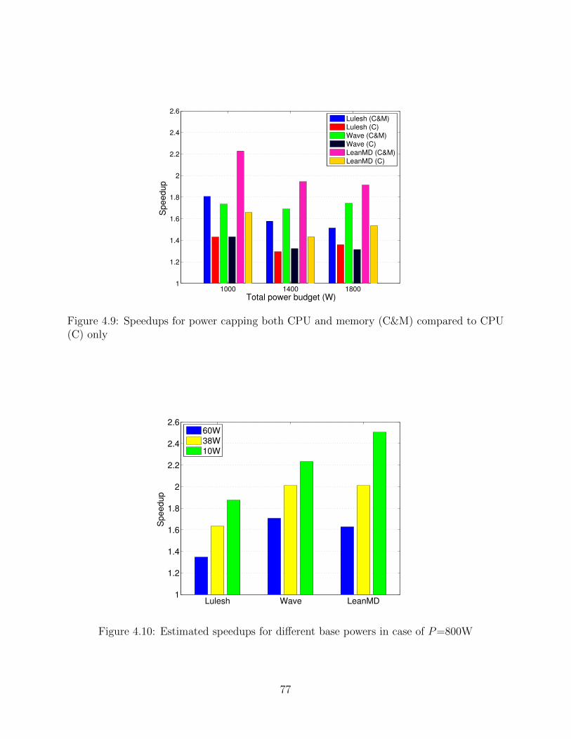
1000 1400 18001
1.2
1.4
1.6
1.8
2
2.2
2.4
2.6
Total power budget (W)
Sp
ee
du
p
Lulesh (C&M)
Lulesh (C)
Wave (C&M)
Wave (C)
LeanMD (C&M)
LeanMD (C)
Figure 4.9: Speedups for power capping both CPU and memory (C&M) compared to CPU(C) only
Lulesh Wave LeanMD1
1.2
1.4
1.6
1.8
2
2.2
2.4
2.6
Sp
ee
du
p
60W38W10W
Figure 4.10: Estimated speedups for different base powers in case of P=800W
77

can expect the speedup of LeanMD to increase from 2 to 2.5. Base power acts as the fixed
cost for adding additional nodes in an over-provisioned system. For example, for P = 800W,
(15×35, 8) and (7×46, 8) are the optimized configurations for LeanMD using base powers of
10W and 60W respectively. For pb = 10W, our model allocates less power to the CPU, i.e.,
pc=35, and uses 15 nodes. However, increasing pb to 60W makes it expensive to add more
nodes. For pb=60W, our model allocates more power to the CPU, i.e., pc=46, while using
only 7 nodes. Hence, the optimized configurations shown in Figure 4.5 would also change
if the base power is changed. As the base power increases (decreases), we expect that the
pc and pm from Figure 4.5 to increase (decrease). We have seen earlier that the optimized
configurations depend on the relationship of execution time with pm and pc. After looking
at Figure 4.10 we can now associate a correlation between optimum configuration and pb as
well. In general, we can conclude that decreasing the base power increases the speedup.
78

CHAPTER 5Job Scheduling Under a Power Budget
In the last chapter we described our interpolation scheme that optimizes execution time for
a single application under a power budget running on an overprovisioned system. In this
chapter, we explore a global power monitoring strategy for high performance computing
(HPC) that addresses optimum power allocation of resources at the data center level. This
chapter builds on the last chapter by applying the lessons learned on a much larger scale,
i.e., allocating resources optimally across a set of jobs.
Currently, some HPC data centers use a FIFO scheme with backfilling to schedule jobs.
While such policies are fair, they do not guarantee throughput maximization of the data
center. In addition, most HPC data centers are unaware of a job’s power characteristics and
hence allocate resources solely on the basis of required number of nodes. In this chapter,
we present a resource management scheme, powered by a novel scheduling methodology
that determines the optimal schedule and resource combination, i.e., number of nodes and
CPU power cap, for the jobs submitted to an HPC data center that maximizes throughput
under a strict power budget. In addition to the scheduling policy, this chapter also describes
a detailed strong scaling power aware model that estimates application execution time for
different resource combinations, i.e., number of nodes and the CPU power level for all of
them. The major contributions of the chapter are:
• An online resource manager (PARM) that uses overprovisioning, power capping and
job malleability along with power-response characteristics of each job for scheduling
and resource allocation decisions that improves the job throughput of the data center
significantly (Section 5.3).
• A performance model that accurately estimates an applications performance for a given
number of nodes and CPU power cap (Section 5.4). We demonstrate the use of our
79
model by estimating characteristics of five applications having different power-response
characteristics (Section 5.5.3).
• An evaluation of our online resource manager on a 38 node cluster with two different job
data sets. A speedup of 1.7 was obtained when compared with SLURM (Section 5.5).
• An extensive simulated evaluation of our scheduling policy for larger machines and
its comparison with the SLURM baseline scheduling policy. We achieve up to 5.2X
speedup operating under a power budget of 4.75 MW (Section 5.6).
5.1 Related work
To the best of our knowledge, this work is the first to employ CPU power capping and
job malleability for improving throughput of an overprovisioned HPC data center. Patki
et al [14] proposed the idea of overprovisioning the compute nodes in power-constrained
high performance computing data centers. They profile an application at different scales
and different CPU power caps. Then they select the best operating configuration for the
application for a given power budget. In Chapter 4 we extended this idea to include memory
power caps and proposed a curve fitting scheme to get an exhaustive profile of an application
at various scales of CPU and memory power caps (within the range of input data). This
profile is then used to obtain the optimal operating configuration of the application under a
strict power budget. Our work proposes a novel scheduling scheme to maximize throughput
under a strict power budget for a data center scheduling multiple jobs simultaneously.
Performance modeling using DVFS has been studied previously [68]. Most of the ex-
isting research estimates execution time based on CPU frequency. These models cannot
be used directly in the context of CPU power capping because applications have different
memory/CPU characteristics can have cores working at different frequencies while operating
under the same CPU power cap. The strong scaling power aware model proposed in this
chapter differs from the work in the previous chapter as it estimates execution time of a
job for a given package power cap that includes the power consumption of cores, caches
and memory controller present on the chip. Researchers have also worked on developing
performance models that capture the energy efficiency of an application [69]. Most of the
energy efficiency work is focussed on optimizing energy consumption. Current data centers
are overprovisioned with respect to power, i.e., each node can be supplied its maximum TDP
power simultaneously, that is seldom needed. Adding more nodes and individually power
capping each node puts the onus on the runtime to ensure that the total power consumption
80

of the data center does not exceed the maximum power that can be supplied to the entire
machine. If the runtime fails to ensure the total power cap, this overdraw may cause the
circuit breakers to trip, which can be costly. Treating power as a constraint can be a much
harder problem than optimizing energy efficiency.
5.2 Data Center and Job Capabilities
In this section, we describe some of the capabilities or features that, according to our un-
derstanding, ought to be present in future HPC data centers. In the following sections, we
highlight the role that these capabilities play for a scheduler that maximizes job throughput
of a data center while ensuring fairness.
Power capping: This feature allows the scheduler to constrain the individual power draw
of each node. Intel’s Sandy Bridge processor family supports on-board power measurement
and capping through the RAPL interface [65]. RAPL is implemented using a series of Ma-
chine Specific Registers (MSRs) that can be accessed to read power usage for each power
plane. RAPL supports power capping Package and DRAM power planes by writing into
the relevant MSRs. Here, ‘Package’ corresponds to the processor chip that hosts processing
cores, caches and memory controller. In this chapter, we use package power interchangeably
with CPU power, for ease of understanding. RAPL can cap power at a granularity of mil-
liseconds which is adequate given that the capacitance on the motherboard and/or power
supply smoothes out the power draw at a granularity of seconds.
Overprovisioning: Capping CPU power below the TDP value using RAPL, allows us to
use more nodes in an overprovisioned data center while staying within the power budget. An
overprovisioned system is thus defined as a system that has more nodes than a conventional
system operating under the same power budget. Due to the additional nodes, such a system
cannot enable all of its nodes to function at their maximum TDP power levels simultane-
ously.
Moldable jobs: In these jobs, user specifies the range of nodes (the minimum and the max-
imum number of nodes) on which the job can run. The job scheduler decides the number
of nodes within the specified range to be allocated to the job. Once decided, the number of
nodes cannot be changed during job execution.
Malleable jobs: Such jobs can shrink to a smaller number of nodes or expand to a larger
number of nodes upon instruction from an external command. Typically, the range of the
nodes in which the job can run is dictated by its memory usage and strong scaling char-
81

acteristics. To enable malleable jobs, two components are critical – a smart job scheduler,
that decides when and which jobs to shrink or expand, and a parallel runtime system that
provides the dynamic contraction and expansion capability to the job. We rely on existing
runtime support for malleable jobs in Charm++ [45]. In Charm++, malleability is achieved
by dynamically exchanging compute objects between processors at runtime. Applications
built on top of such an adaptive system have been shown to shrink and to expand with small
costs [70]. Charm++ researchers are currently working on further improving the support for
malleable jobs. Malleability support in MPI applications has been demonstrated in earlier
work [71].
5.3 The Resource Manager
Figure 5.1 shows the block diagram of our online Power Aware Resource Manager, or PARM.
It has two major modules: the scheduler and the execution framework. The scheduler is
responsible for identifying which jobs should be scheduled and exactly what resources should
be devoted to each job. We refer to the resource allocation for each job by the resource
combination tuple, (n, p), where n is the number of nodes and p is the CPU power cap for
each of the n nodes. The scheduling decision is made based on the Integer Linear Program
(ILP), and the job profiles generated by our strong scaling power aware model described in
Section 5.4. The scheduler’s decisions are fed as input to the execution framework, which
implements/enforces them by launching new jobs, shrinking/expanding running jobs, and/or
setting the power caps on the nodes.
The scheduler is triggered whenever a new job arrives or when a running job ends or
abruptly terminates due to an error or any other reason (‘Triggers’ box in Figure 5.1). At
each trigger, the scheduler tries to re-optimize resource allocation to the set of pending as
well as currently running jobs with the objective of maximizing overall throughput. Our
scheduler uses both CPU power capping and moldability/malleability features for through-
put maximization. We formulate this resource optimization problem as an Integer Linear
Program (ILP). The relevant terminology is described in Table 5.1. Our scheduling scheme
can be summarized as:
Input: A set of jobs that are currently executing or are ready to be executed (J ) with
their expected execution time corresponding to a set of resource combinations (n, p), where
n ∈ Nj and p ∈ Pj.Objective: Maximize data center throughput.
Output: Allocation of resources to jobs at each trigger event, i.e., identification of the jobs
82

`"Job"Arrives" Job"Ends/Terminates"
Schedule"Jobs"(LP)"
Update"Queue"
Scheduler"
Launch"Jobs/"ShrinkAExpand"
Ensure"Power"Cap"
ExecuEon"framework"
Triggers"
Profiler"
Strong"Scaling"Power"Aware"Model"
Job"CharacterisEcs"Database"
Power"Aware"Resource"Manager"(PARM)"
Figure 5.1: A high level overview of PARM
that should be executed along with their resource combination (n,p).
5.3.1 Integer Linear Program Formulation
We make the following assumptions and simplifications in the formulation:
• All nodes of a given job are allocated the same power.
• We do not include cooling power of the data center in our calculations.
• Job characteristics do not change significantly during the course of its execution.
• Expected wall clock time and the actual execution time are equal for the purpose of
decision making by the scheduler.
• Wbase, that includes power for all components of a node other than the CPU and
memory subsystems, is assumed to be constant.
• A job once selected for execution is not stopped until its completion, although the
resources assigned to it can change during its execution.
83

Variable Description
N total number of nodes in the data centerJ set of all jobsI set of jobs that are currently runningI set of jobs in the pending queueJ set of jobs that have already arrived
and have not yet been completed, i.e., theyare either pending or currently running, J = I ∪ I
Nj set of node counts on which job j can be runPj set of power levels at which job j should be run or
in other words, the power levels at which job j’sperformance is known
nj number of nodes at which job j is currently runningxj,n,p binary variable, 1 if job j should run
on n nodes at power p, otherwise 0tnow current timetaj arrival time of job j
Wbase base machine power that includes everythingother than CPU and memory
tj,n,p execution time for job j running on nnodes with a power cap of p
sj,n,p strong scaling power aware speedup of application jrunning on n nodes with a power cap of p
min(Nj) minimum number of nodes that can be assigned to job jmin(Pj) minimum amount of power that can be assigned to job j
Table 5.1: Integer Linear Program Terminology
• All jobs are from a single user (or have the same priority). This condition can be
relaxed by introducing appropriate priority factors in the objective function of the
ILP.
Scheduling problems are framed as ILPs and ILPs are NP-hard problems. Maximizing
throughput in the objective function requires introducing variables for the start and end
time of jobs. These variables make the ILP computationally very intensive and thus im-
practical for online scheduling in many cases. In this work, we propose to drop the job start
and end time variables and take a greedy approach by selecting jobs and resource alloca-
tions that maximizes the sum of the power-aware speedup (described later) of selected jobs.
This objective function improves the job throughput while keeping the ILP optimization
computationally tractable for online scheduling.
84

Objective Function∑j∈J
∑n∈Nj
∑p∈Pj
wj ∗ sj,n,p ∗ xj,n,p (5.1)
Select One Resource Combination Per Job∑n∈Nj
∑p∈Pj
xj,n,p ≤ 1 ∀j ∈ I (5.2)
∑n∈Nj
∑p∈Pj
xj,n,p = 1 ∀j ∈ I (5.3)
Bounding total nodes∑j∈J
∑p∈Pj
∑n∈Nj
nxj,n,p ≤ N (5.4)
Bounding power consumption∑j∈J
∑n∈Nj
∑p∈Pj
(n ∗ (p+Wbase))xj,n,p ≤Wmax (5.5)
Disable Malleability (Optional)∑n∈Nj
∑p∈Pj
nxj,n,p = nj ∀j ∈ I (5.6)
Figure 5.2: Integer Linear Program formulation of PARM scheduler
We define the strong scaling power-aware speedup of a job j as follows:
sj,n,p =tj,min(Nj),min(Pj)
tj,n,p(5.7)
where sj,n,p is the speedup of job j executing using resource combination (n, p) with respect
to its execution with resource combination (min(Nj),min(Pj)). Objective function (Eq. 5.1)
of the ILP maximizes the sum of the power-aware speedups of the jobs selected for execution
at every trigger event. This leads to improvement in FLOPS/Watt (or power efficiency, as
we define it). Improved power efficiency implies better job throughput (results discussed in
Section 5.5, 5.6). Oblivious maximization of power efficiency may lead to starvation for jobs
with low strong scaling power aware speedup. Therefore, to ensure fairness, we introduced
a weighing factor (wj) in the objective function, which is defined as follows:
wj = (tremj,min(Nj),min(Pj) + (tnow − taj ))α (5.8)
wj artificially boosts the strong scaling power aware speedup of a job by multiplying it to the
job’s completion time, where completion time is the sum of the time elapsed since the job’s ar-
85

rival and the job’s remaining execution time with resource combination (min(Nj),min(Pj))
i.e. (tremj,min(Nj),min(Pj)) . The percentage of a running job completed between two successive
triggers is determined by the ratio of the time interval between the two triggers and the
total time required to complete the job using its current resource combination. Percentage
of the job that has been completed so far can then be used to compute tremj,min(Nj),min(Pj). The
constant α (α ≥ 0) in Eq. 5.8 determines the priority given to job fairness against its strong
scaling power aware speedup i.e. a smaller value of α favors job throughput maximization
while a larger value favors job fairness.
We now explain the constraints of our ILP (Figure 5.2):
• Select one resource combination per job (Eq. 5.2,5.3): xj,n,p is a binary variable indi-
cating if job j should run using resource combination (n, p). This constraint ensures
that at most one of the variables xj,n,p is set to 1 for any job j. The jobs that are
already running (set I) continue to run although they can be assigned a different re-
source combination (Eq. 5.3). The jobs in the pending queue (I), for which at least
one of the variables xj,n,p is equal to 1 (Eq. 5.2), are selected for execution and moved
to the set of jobs currently running (I).
• Bounding total nodes (Eq. 5.4): This constraint ensures that the number of active
nodes does not exceed the maximum number of nodes available in the overprovisioned
data center.
• Bounding power consumption (Eq. 5.5): This constraint ensures that power consump-
tion of all nodes does not exceed the power budget of the data center.
• Disable Malleability (Eq. 5.6): To quantify the benefits of malleable jobs, we consider
two versions of our scheduler. The first version supports only moldable jobs and is
called as noSE (i.e. no Shrink/Expand), The second version allows both moldable and
malleable jobs and is called as wSE (i.e. with Shrink/Expand). Malleability can be
disabled by using Eq. 5.6. This constraint ensures that the number of nodes assigned
to each running job does not change during the optimization process. However, it
allows changing the power allocated to running jobs. In real-world situations, the jobs
submitted to a data center will be a mixture of malleable and non-malleable jobs. The
scheduler can apply Eq. 5.6 to disable malleability for non-malleable jobs.
86

5.4 Strong Scaling Power Aware Model
Recent processors allow power capping, which gives a new dimension to performance model-
ing. In this section, we propose a strong scaling power-aware model, by extending Downey’s [72]
strong scaling model and making it power aware. The goal is to develop a model that can
estimate the execution time of an application for any given resource combination (n, p).
5.4.1 Strong Scaling Model
We used Downey’s [72] strong scaling model after modifying the boundary conditions. An
application can be characterized by an average parallelism of A. The application’s paral-
lelism remains equal to A, except for a fraction σ of total execution time . The variance of
parallelism, represented as V = σ(A− 1)2, depends on σ, where 0 ≤ σ ≤ 1. The execution
time, t(n), of an application can then be defined as follows:
t(n) =
T1 − T1σ2A
n+T1σ
2A, 1 ≤ n ≤ A (5.9)
σ(T1 − T12A
)
n+T1A− T1σ
2AA < n ≤ 2A− 1 (5.10)
T1A, n < 2A− 1 (5.11)
where n is the number of nodes and T1 is the execution time on a single node. Since we have
to estimate execution time corresponding to different number of nodes n given t(1) = T1,
we had to modify Downey’s model according to boundary condition t(1) = T1. The first
equation in this group represents the range of n where applications are most scalable. This is
the range where the number of nodes is less than A, i.e., the average amount of parallelism.
The application’s scalability declines significantly once n becomes larger than A because
some nodes are unable to do work in parallel owing to a lack of parallelism. Finally, for
n > 2A, the execution time t(n) equals T1/A and does not decrease. Given application
characteristics σ, A, and T1, this model can be used to estimate execution time for any
number of nodes n.
5.4.2 Adding Power Awareness to the Strong Scaling Model
The effect of increasing frequency on the execution time t varies from application to appli-
cation [61] . In this section, we first describe a basic framework that models t as a function
87

of CPU frequency f . Since, f can be expressed as a function of CPU power p, we can finally
express t in terms of p.
Execution Time as a Function of Frequency
Existing work [61] indicates that an increase in CPU frequency beyond a certain threshold
frequency, fh, does not reduce the execution time t. The value of fh depends on the memory
bandwidth being used by the application. Since t ∝ 1f, we can express t as [68]:
t(f) =
W
f+ T, for f < fh (5.12)
Th, for f ≥ fh (5.13)
where W and T are constants that roughly correspond to the CPU and memory bounded
work respectively. Th is the execution time at frequency fh. Given that fl is the smallest
possible frequency at which a CPU can operate, Equation 5.12 should obey the boundary
conditions t(fl) = Tl and t(fh) = Th where Tl is the execution time while operating at the
minimum frequency level (fl).
We define parameter β that characterizes the frequency-sensitivity of an application and
can be expressed as:
β =Tl − ThTl
(5.14)
The range of β depends on the CPU’s DVFS range. Given the DVFS range of (fl, fmax),
β ≤ 1− flfmax
. Typically, CPU-bound applications have higher values for β whereas memory-
intensive applications have smaller β values.
Using Equation 5.14 and subjecting Equation 5.12 to boundary conditions, t(fl) = Tl and
t(fh) = Th, gives us:
W =Thβflfh
(1− β)(fh − fl)(5.15)
T = Th −Thβfl
(1− β)(fh − fl)(5.16)
Execution Time as a Function of CPU Power
Although Intel has not released complete details of the CPU power capping functionality, it
has been hinted that the power cap is ensured by using a combination of DVFS and CPU
throttling. Core input voltage and frequency can be set within manufacturer defined ranges.
This frequency-voltage range, in turn, defines a range over CPU power that can be achieved
88

using DVFS. Let pl denote the CPU power corresponding to fl, where fl is the minimum
frequency the CPU can operate at using DVFS. Beyond pl, power is reduced by mechanisms
other than DVFS, e.g., CPU throttling. The threshold pl, where CPU throttling takes over
from DVFS, can be determined by looking at the processor’s operating frequency. CPU or
package power includes the power consumption by its various components such as cores,
caches, and memory controller. The value of pl varies depending on an application’s usage
of these components. In a CPU bound application, a processor might be able to cap power
to lower values using DVFS, since only the cores are consuming power. In contrast, for a
memory intensive application, pl might be higher, since the caches and memory controller
are also consuming power in addition to the cores. Since core input voltage is proportional
to f , power consumption of the cores, pcore, can be modeled as:
pcore = Cf 3 +Df (5.17)
where C and D are constants. Since the number of cache and memory accesses are pro-
portional to frequency, DVFS can change cache/memory controller power consumptions as
well. The CPU power can then be expressed as [73]:
p = pcore +3∑i=1
giLi + gmM + pbase (5.18)
where Li is accesses per second to level i cache, gi is the cost of a level i cache access (in
W), M is the number of memory accesses per second, gm is the cost per memory access (in
W), and pbase is the base package power consumption. Equation 5.18 can also be written as:
p = F (f) = af 3 + bf + c (5.19)
where a, b, and c are constants. In Equation 5.19, the term bf corresponds to the cores’
leakage power and the power consumption of the caches and the memory controller. The
term af 3 represents the dynamic power of the cores, whereas c = pbase is the base CPU power.
The constants a and b are application dependent since the cache and memory behavior can be
different across applications. Equation 5.19 can be rewritten as a depressed cubic equation:
f 3 +b
af +
c− pa
= 0 (5.20)
89

and solved using Fermat’s Last Theorem to get F−1:
f = F−1(p) =3
√p− c
2a+
√(p− c)2
4a2+
b3
27a3
+3
√c− p
2a+
√(p− c)2
4a2+
b3
27a3(5.21)
To express t in terms of p, we use Equation 5.21 to replace f , fl, and fh in Equations 5.12,
5.15, 5.16. To combine our power aware model with the strong scaling model described in
Section 5.4.1, we replace Th in Equations 5.12, 5.15, 5.16 with t(n) from Equations 5.9, 5.10,
5.11.
Summary: We present a comprehensive model to estimate t for any resource combination
(n, p), given application parameters σ, T1, A, pl, ph, β, a and b. We substitute parameters
σ, T1 and A into Equations 5.9, 5.10, 5.11 to determine t = t(n), i.e., execution time using n
nodes working at maximum power. We then use Th = t(n) and parameters pl, ph, β, a and b
to determine t(n, p) using Equations 5.12, 5.15, 5.16, and 5.21, i.e., execution time using n
nodes operating at p Watts each.
5.5 Experimental Results
In this section, we describe our experimental setup that includes applications, testbed, and
job datasets. We obtain the application characteristics using the power-aware strong-scaling
performance model and finally compare the performance of the noSE and wSE versions of
PARM with SLURM.
5.5.1 Applications
We used five applications, namely, Wave2D, Jacobi2D, LeanMD, Lulesh, and Adaptive Mesh
Refinement or AMR [74]. These applications have different CPU and memory usage:
• Wave2D and Jacobi2D are 5-point stencil applications that are memory-bound. Wave2D
has higher FLOPS than Jacobi2D.
• LeanMD is a computationally intensive molecular dynamics application.
• CPU and memory usage of Lulesh and AMR lies in between the stencil applications
and LeanMD.
90

5.5.2 Testbed
We conducted our experiments on a 38-node Dell PowerEdge R620 cluster (which we call
the Power Cluster). Each node containing an Intel Xeon E5-2620 Sandy Bridge with 6
physical cores at 2GHz, 2-way SMT with 16 GB of RAM. These machines support on-board
power measurement and capping through the RAPL interface [36]. The CPU power for our
testbed can be capped in the range [25− 95]W , while the capping range for memory power
is [8− 35]W .
5.5.3 Obtaining Model Parameters of Applications
Application characteristics depend on the input type, e.g., gird size. We fix the respective
input types for each application. Each application needs to be profiled for some (n,p) combi-
nations to obtain data for curve fitting. 1 step/iteration is sufficient to get the performance
for a given data point. Since, a step/iteration is usually of the order of milliseconds, the
cost of profiling the application at several data points is negligible compared to the overall
execution time of the application.
We use linear and non-linear regression tools provided by MATLAB to determine the ap-
plication parameters by fitting the sampled application performance data to the performance
model proposed in Section 5.4. Figure 5.3 (a-e) shows the observed (dots) and estimated
(lines) execution time corresponding to different CPU power caps for all applications when
run on 20 nodes of our Power Cluster. In all cases, the fitted curves match the observed
data with a Root Mean Square Error (RMSE) percentage of less than 2%. The obtained
parameter values for all applications are listed in Table 5.2 and are discussed here:
• The parameter c (CPU base power) lies in the range [13− 14]W for all applications
• pl was 30W for LeanMD and 32W for rest of applications. For LeanMD, it is possible
to cap the CPU power to a lower value just by decreasing the frequency using DVFS.
This is because LeanMD is a computationally intensive application and therefore most
of the power is consumed by the cores rather than caches and memory controller. On
the contrary, for other applications, CPU throttling kicks in at a higher power level
because of their higher cache/memory usage.
• value of ph lies in the range of [37− 54]W for applications under consideration.
• value of β lies in the range [0.08− 0.40]. Higher value of β means higher sensitivity to
CPU power.
91
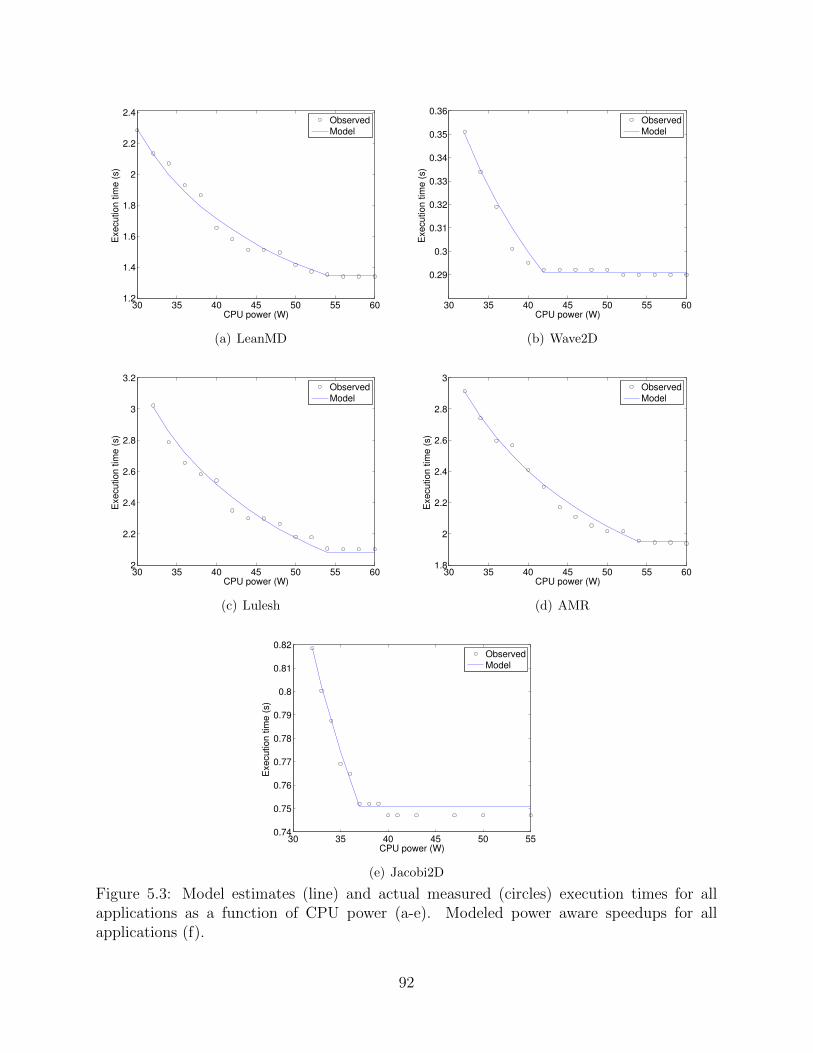
30 35 40 45 50 55 601.2
1.4
1.6
1.8
2
2.2
2.4
CPU power (W)
Execution tim
e (
s)
Observed
Model
(a) LeanMD
30 35 40 45 50 55 60
0.29
0.3
0.31
0.32
0.33
0.34
0.35
0.36
CPU power (W)
Execution tim
e (
s)
Observed
Model
(b) Wave2D
30 35 40 45 50 55 602
2.2
2.4
2.6
2.8
3
3.2
CPU power (W)
Execution tim
e (
s)
Observed
Model
(c) Lulesh
30 35 40 45 50 55 601.8
2
2.2
2.4
2.6
2.8
3
CPU power (W)
Execution tim
e (
s)
Observed
Model
(d) AMR
30 35 40 45 50 550.74
0.75
0.76
0.77
0.78
0.79
0.8
0.81
0.82
CPU power (W)
Execution tim
e (
s)
Observed
Model
(e) Jacobi2D
Figure 5.3: Model estimates (line) and actual measured (circles) execution times for allapplications as a function of CPU power (a-e). Modeled power aware speedups for allapplications (f).
92

30 35 40 45 50 55 601
1.1
1.2
1.3
1.4
1.5
1.6
1.7
1.8
CPU power (W)
Po
we
r−a
wa
re s
pe
ed
up
LeanMDLuleshWave2DJacobi2D
Figure 5.4: Modeled (lines) and observed (markers) power aware speedups for four applica-tions
• Wave2D and Jacobi2D have the largest memory footprint that results in high CPU-
cache-memory traffic. Therefore the value of b is high for these two applications.
Figure 5.4 shows the modeled (lines) as well as the observed (markers) power-aware
speedups for 4 applications under consideration. Since AMR’s characteristics are very sim-
ilar to Lulesh, we leave AMR out to improve the clarity of the figure. Each application’s
speedup was calculated with respect to the execution time when that application was exe-
cuting at p = pl. LeanMD has the highest power-aware speedup whereas Jacobi2D has the
lowest.
5.5.4 Power Budget
We assume a power budget of 3300W to carry out experiments using our Power Cluster.
Although the vendor-specified TDP of CPU and memory of the Dell nodes was 95W and
35W, respectively, the actual power consumption of CPU and memory never went beyond
60W and 18W, respectively, when running any of the applications. Therefore, instead of
93

Application a b pl ph β
LeanMD 1.65 7.74 30 52 0.40Wave2D 3.00 10.23 32 40 0.16Lulesh 2.63 8.36 32 54 0.30AMR 2.45 6.57 32 54 0.33Jacobi2D 1.54 10.13 32 37 0.08
Table 5.2: Obtained model parameters
the vendor-specified TDP, we consider 60W and 18W as the maximum CPU and memory
power consumption and use them to calculate the number of nodes that can be installed
in a traditional data center. The maximum power consumption of a node, thus, adds up
to 60W + 18W + 38W = 116W , where 38W is the base power of a node. Therefore,
the total number of nodes that can be installed in a traditional data center with a power
budget of 3300W will be b3300116c = 28 nodes. By capping the CPU power below 60W, the
overprovisioned data center will be able to power more than 28 nodes.
5.5.5 Job Datasets
We constructed two job datasets by choosing a mix of applications from the set described in
Section 5.5.1. All these applications are written using the Charm++ parallel programming
model and hence support job malleability. Application’s power-response characteristics can
influence the benefits of PARM. Therefore, in order to better characterize the benefits of
PARM, these two job datasets were constructed such that they have very different average
values of β. We name these datasets as SetL and SetH, with average β value of 0.1 and 0.27,
respectively. For instance, SetH has 3 LeanMD, 3 Wave2D, 2 Lulesh, 1 Jacobi, and 1 AMR
job, that gives us an average β value of 0.27. A mix of short, medium and long jobs were
constructed by randomly generating wall clock times with a mean value of 1 hour. Similarly,
the job arrival times were generated randomly. Each dataset spans over 5 hours of cluster
time and approximately 20 scheduling decisions were taken (a scheduling decision is taken
whenever a new job arrives or a running job terminates). The minimum and the maximum
number of nodes on which a job can run was determined by the job’s memory requirements.
We used 8 node levels (i.e. |Nj| = 8) that are uniformly distributed between the minimum
and maximum number of nodes on which the job can run. The memory power is capped at
the fixed value of 18W whereas we used 6 CPU power levels - [30, 32, 34, 39, 45, 55]W.
94

5.5.6 Performance Metric
We compare our scheduler with SLURM [75]: an open-source resource manager that allocates
compute nodes to jobs and provides a framework for starting, executing and monitoring jobs
on a set of nodes. SLURM provides resource management on many of the most powerful
supercomputers of the world including Tianhe-1A, Tera 100, Dawn, and Stampede. We
setup both PARM and SLURM on the testbed. For comparison purpose, we use SLURM’s
baseline scheme in which the user specifies the exact number of nodes requested for the job
and SLURM uses FIFO + backfilling for making scheduling decisions. We call this as the
SLURM baseline scheme or just the baseline scheme. The number of nodes requested for a
job submitted to SLURM is the minimum number of nodes on which PARM can run that
job.
We use response time and completion time as the metrics for comparing PARM and
SLURM. A job’s response time, tres, is the time interval between its arrival and the beginning
of its execution. Execution time, texe, is the time from start to finish of a job’s execution.
Completion time, tcomp, is the time between a job’s arrival and the time that it finishes
execution, i.e., tcomp = tres + texe. Job throughput is the inverse of the average completion
time of jobs. In this study, we emphasize on completion time as the performance comparison
metric, even though typically response time is the preferred metric. This is because unlike
conventional data centers, where resources allocated to a job and hence the jobs execution
time are fixed, our scheduler dynamically changes job configuration during execution which
can vary job execution time significantly. Hence, response time is not a very appropriate
metric for comparison in this study. Completion time includes both the response time and
the execution time and is therefore the preferred metric of comparison.
5.5.7 Results
Figure 5.5(a) shows the average completion times of the two datasets with SLURM and
the noSE and wSE versions of PARM. The completion times for wSE and noSE include
all overhead costs including the ILP optimization time and the costs of constriction and
expansion of jobs. As noted in the figure, PARM significantly reduces the average completion
time for both the data sets. This improvement can mainly be attributed to the reduced
average response times shown in Figure 5.5(b). Our scheduler intelligently selects the best
power levels for each job which allows it to add more nodes to benefit from strong scaling
and/or scheduling more jobs simultaneously. The completion times of wSE scheme are better
than noSE. Job malleability allows wSE scheme to shrink and expand jobs at runtime. This
95

SetL SetH0
50
100
150
200
250
300
Ave
rag
e c
om
ple
tio
n t
ime
(m
ins)
SLURMnoSEwSE
(a) Average completion time
SetL SetH0
50
100
150
200
250
300
Ave
rag
e r
esp
on
se
tim
e (
min
s)
SLURMnoSEwSE
(b) Average response time
0
5
10
15
20
25
30
35
40
45
SetL SetH 0
10
20
30
40
50
Ave
rage
num
. of n
odes
Ave
rage
CP
U p
ower
(W)
Avg. nodes wSEAvg. nodes noSE
Avg. CPU power wSEAvg CPU power noSE
(c) Average nodes and average power per nodeFigure 5.5: (a) Average completion times, and (b) average response times for SetL and SetHwith SLURM and noSE, wSE versions of PARM. (c) Average number of nodes and averageCPU power in the wSE and noSE versions of PARM.
96

gives flexibility to the ILP to re-optimize the allocation of nodes to the running and pending
jobs. On the other hand, noSE reduces the solution space of ILP by not allowing running
jobs to change the number of nodes allocated to them. Additionally, wSE increases the
machine utilization towards the tail of the job dataset execution when there are very few
jobs left running. The wSE version can expand the running jobs to run on the unutilized
machines. These factors reduce both the average completion and the average response time
in wSE (Figure 5.5(a), 5.5(b)). As shown by Figure 5.5(c), wSE scheme utilizes 36 nodes on
an average compared to an average of 33 nodes used in the case of noSE for SetL.
A smaller value of β means that effect of decreasing the CPU power on application per-
formance is small. When β is small, the scheduler will prefer to allocate less CPU power
and use more nodes. On the other hand, when β is large, the benefits of adding more nodes
at the cost of decreasing the CPU power are smaller. The flexibility to increase the number
of nodes gives PARM higher benefit over SLURM when β is small as compared to the case
when β is large. Therefore, lower the sensitivity of applications to the allocated CPU power
(i.e. smaller value of β), higher will be the benefit of using PARM. This is corroborated
with the observation (Figure 5.5) that the benefits of using PARM as compared to SLURM
are much higher with dataset SetL (β = 0.1) as compared to dataset SetH (β = 0.27).
5.6 Large Scale Projections
After experimentally showing the benefits of PARM on a real cluster, we now analyze its
benefit on very large machines. Since doing actual job scheduling on a large machine is
practically infeasible for us, we use the SLURM simulator [76], which is a wrapper around
SLURM. This simulator gives us information about SLURM’s scheduling decisions without
actually executing the jobs. In the following subsections, we describe our shrink/expand
cost model, give the experimental setup and then present a comparison of PARM scheduling
with SLURM baseline scheduling policy.
5.6.1 Modeling Cost of Shrinking and Expanding Jobs
Constriction and expansion of jobs has an overhead associated with it. These overheads come
from data communication done to balance the load across the new set of processors assigned
to the job and from the boot time of nodes. A scheduler typically makes two decisions: 1)
how many nodes to assign to each job, and 2) which nodes to assign to each job. We address
the first decision in this paper and defer the second for future work. Let us say that job j
97

with a total memory of mj MB, has to expand from nf nodes to nt nodes. For simplification
of analysis, we assume that each job is initially allocated a cuboid of nodes (with dimensions-
3√nf × 3
√nf × 3
√nf ) interconnected through a 3D torus. After the expand operation, size of
the cuboid becomes 3√nf × 3
√nf × nt
23√nf
. For load balance, the data in memory (mj MB)
will be distributed equally among the nt nodes. Hence, the communication cost for the data
transfer can be expressed as tc (in seconds):
tc =(mjnf− mj
nt) ∗ nf
2 ∗ b ∗ n23f
(5.22)
where b is the per link bandwidth. The numerator in Eq. 5.22 represents the total data to
be transferred whereas the denominator represents the bisection bandwidth of the cuboid.
Similarly, the cost of shrinking a job is determined by computing the cost of distributing the
data of nf − nt nodes equally across the final nt nodes.
Boot times can be significant for some supercomputers. Since many supercomputers in
Top500 [13] belong to the Blue Gene family, we include their boot time when evaluating our
scheme. We adopt a simple linear model to calculate the boot time (tb) for expand operation.
The following linear relationship is obtained by using the Intrepid boot time data [77]:
tb(in seconds) = (nt − nf ) ∗ 0.01904 + 72.73 (5.23)
In an expand operation, communication phase can start only after additional nodes be-
come available. These additional nodes might have to be booted. Therefore the total cost
of a shrink or expand operation is sum of the boot time and the data transfer time, i.e.,
tse = tc + tb. A job set for expansion might receive additional nodes from a job undergoing
constriction in the same scheduling decision. Therefore, an expanding job has to wait until
the shrinking job has released the additional resources. To simplify this analysis, we deter-
mine the maximum tse from among the shrinking/expanding jobs (tmaxse ) and add 2tmaxse to
the execution times of all jobs that shrink or expand due to the current scheduling decision.
To control the frequency of constriction or expansion of a job, and consequently its cost,
we define a parameter fse (in secs). fse is the time after which a job can shrink or expand,
i.e., if a job was shrunk or expanded at t secs, then it can be shrunk or expanded only after
t+ fse secs. This condition is enforced using Eq. 5.6.
98

5.6.2 Experimental Setup
The results presented in this section are based on the job logs [78] of Intrepid. Intrepid is
a IBM BG/P supercomputer with a total of 40, 960 nodes, installed at Argonne National
Lab. The job trace spans over 8 months and has 68, 936 jobs. We extracted 3 subsets of
1000 successive jobs each from the trace file to conduct our experiments. These subsets will
be referred to as Set1, Set2, and Set3 and the starting job id for these subsets are 1, 10500,
and 27000, respectively. To measure the performance of PARM in the wake of diverse job
arrival rates, we generated several other datasets from each of these sets by multiplying the
arrival times of each job by γ, where γ ∈ [0.2− 0.8]. Multiplication of the arrival times with
γ increases the job arrival rate without changing the distribution of job arrival times.
As we do not know application characteristics (σ, T1, A, fl,
fh, β, a and b) of the jobs in the Intrepid trace file, we take the parameter values from
Section 5.5.3 and randomly assign values from these ranges to jobs in the Intrepid trace
file. Since Intrepid does not allow moldable/malleable jobs, jobs request a fixed number
of nodes instead of a range of nodes. For jobs submitted to the PARM scheduler, we
consider this number as the maximum nodes that the job is allowed to use, i.e., max(Nj)
and set min(Nj) = θ ∗max(Nj), where θ is randomly selected in the range [0.2− 0.6]. The
power consumption of Intrepid nodes is not publicly available, therefore we use the power
values from our testbed cluster (described in Section 5.5.2). Hence, the maximum power
consumption per node is taken to be 116W. The maximum power consumption of 40, 960
nodes thus equals 116× 40, 960 = 4, 751, 360W. The SLURM scheduler schedules on 40, 960
nodes with each node running at maximum power level. As in Section 5.5.5, PARM uses 6
CPU power levels, Pj = {30, 33, 36, 44, 50, 60}W .
5.6.3 Performance Results
Both noSE and wSE significantly reduce average completion times compared to SLURM’s
baseline scheduling policy (Figure 5.6). As γ decreases from 0.8 to 0.2, the average com-
pletion time increases in all the schemes because the jobs arrive at a much faster rate and
therefore have to wait in the queue for longer time before they get scheduled. However, this
increase in the average completion times with both our schemes is not as significant as it is
with the baseline scheme.
Both noSE and wSE have significantly improved average response times, with wSE out-
performing noSE (Table 5.3). Execution time in wSE includes the costs of shrinking or
expanding the job (Section 5.6.1). Despite this overhead, wSE outperforms noSE in average
99

0.8 0.7 0.6 0.5 0.4 0.3 0.20
100
200
300
400
500
600
700
Arrival time scaling factor (γ)
Ave
rag
e c
om
ple
tio
n t
ime
(m
ins)
baselinenoSEwSE
(a) Set1
0.8 0.7 0.6 0.5 0.4 0.3 0.20
100
200
300
400
500
600
700
Arrival time scaling factor (γ)
Ave
rag
e c
om
ple
tio
n t
ime
(m
ins)
baselinenoSEwSE
(b) Set2
0.8 0.7 0.6 0.5 0.4 0.3 0.20
100
200
300
400
500
600
700
Arrival time scaling factor (γ)
Ave
rag
e c
om
ple
tio
n t
ime
(m
ins)
baselinenoSEwSE
(c) Set3
Figure 5.6: Average completion times of baseline, noSE and wSE. Job arrival times in allthe sets (Set1, Set2, Set3) were scaled down by factor γ to get diversity in job arrival rate
100

SetAvg Resp. Time (mins) Avg Exe. Time (mins) Avg. Num. of Nodes Speedupbaseline wSE noSE baseline wSE noSE baseline wSE noSE wSE noSE
1 (γ = 0.5) 90 3 6 80 84 95 453 610 601 1.91 1.702 (γ = 0.5) 500 34 57 57 69 89 632 714 721 5.25 4.663 (γ = 0.5) 217 99 88 60 73 90 520 662 665 1.65 1.612 (γ = 0.7) 142 12 20 57 66 83 596 656 660 2.36 1.963 (γ = 0.7) 194 95 86 60 73 90 488 596 599 1.54 1.43
Table 5.3: Comparison of the baseline, wSE and noSE scheduling policies for different datasets.
execution time of jobs. wSE version consistently outperforms noSE in all data sets. The
average completion times reported in Figure 5.6) includes cost of all overheads. In all the job
datasets, the average overhead for shrinking and expanding the jobs was less than 1% of the
time taken to execute the dataset. We controlled these costs by setting fse = 500 secs, i.e.,
the scheduler waited for at least 500 secs between two successive contraction and expansion
operations for a job. We found the cost for solving the ILP to be small. The largest ILP that
we solved took 15 secs which is negligible given the frequency at which the scheduler was
invoked is much smaller. We use data from Table 5.3 to explain two observations related to
the speedups of our schemes. The speedup in average completion time for both our policies
is calculated relative to the baseline (shown in Table 5.3).
• Higher speedup in average completion time for γ = 0.5 compared to γ = 0.7 in
Set2: The baseline case has a 4 fold increase in response time compared to just a
2 fold increase in response time for wSE when γ changes from 0.7 to 0.5. Average
execution time in the wSE version increases only slightly after γ changes from 0.7 to
0.5 (Table 5.3), while it remains constant in the baseline scenario. Since, completion
time is the sum of response and execution time, we observe higher speedups for smaller
values of γ in Set2.
• Smaller speedups in Set3 as compared to Set2: Upon job trace inspection, we discovered
that there are not enough jobs to keep the machine fully utilized during the first half
of Set3. Therefore, even after reducing γ to small values, the response time is not
significantly affected in Set3. In contrast, Set2 has a very high machine utilization
which leads to a significant increase in the response time of the baseline scheduler as
γ is reduced (from 0.5 to 0.7), resulting in higher speedups for both our scheduling
policies.
To see the effectiveness of our scheme, we compared it with a baseline scheduler if it were
to schedule jobs on an overprovisioned system. All CPUs in this system are power capped
at the same value (< 60W). This allows the baseline scheduler to add more nodes while
remaining within the same power budget, e.g., setting the power cap for each CPU to 30W
101

CPU power cap (W) 30 40 50 60
Speedup 4.32 1.86 2.33 5.25Avg number of nodes 50332 42486 39700 37956
Table 5.4: Comparison of wSE with the baseline scheduler running on an overprovisionedsystem (at different CPU power caps) using Set 2 (γ = 0.5)
allows baseline (SLURM) to use up to b 4,751,36030+18+38
c = 55, 248 nodes. In Table 5.4, we present
the speedup of wSE relative to a baseline scheduler operating on an overprovisioned system
with different CPU power caps as the reference. Significant speedups in Table 5.4 emphasize
the benefits of solving the ILP for determining optimal job configurations rather than using
the baseline scheduler, which runs all jobs at the same node power. Table 5.4 shows that
even after scheduling on an overprovisioned system and using greater than 40,960 nodes, the
baseline scheduler still under performs our scheduler by a significant margin.
5.6.4 Increasing Job Arrival Rate While Maintaining the Same QoS
For the purpose of this study we define the Quality of Service (QoS) for a data center to
be determined by the average and maximum completion time of its jobs. To emphasize the
usefulness of our schedulers, we increased the arrival rate of jobs (by multiplying the original
arrival times by the constant γ) as much as possible, so long as we maintain the same QoS
as provided by the baseline schedule (γ = 1). The results are presented in Figure 5.7).
Consider the first group of bars: wSE allowed for arrival time of the last job of Set1 to be
reduced to just 2.2 days and still provided the same QoS as the baseline scheduler whose
last job arrived at 6.8 days (arrival times of other jobs are scaled down proportionately)..
Similarly trends may be seen in Figure 5.7 for the other sets.
5.6.5 Analyzing tradeoff between Fairness and Throughput
We introduced the term wj in the objective function of the scheduler’s ILP (Equation 5.1)
to prevent starvation of jobs with low power-aware speedup. In this section, we analyze the
tradeoff between maximum completion time of any job (fairness) and the average completion
time of jobs (equivalent to throughput). The parameter α can be be tuned by the data
center administrator to control fairness and throughput. We performed several experiments
by varying α and measured its impact on the average and maximum completion times.
Figure. 5.8 and Figure. 5.8 plot the average and maximum completion times of Set2 for
102

Set 1 Set 2 Set 30
0.2
0.4
0.6
0.8
1
γ
noSE
wiSE
Figure 5.7: Reduction in job arrival times while maintaining the same QoS as the baselinescheduler
different values of α using γ = 0.8. As the value of α increases, the maximum completion time
decreases at the cost of an increase in average completion time (Figure. 5.8 and Figure. 5.9).
We further compare completion times of our scheduler with the baseline. Figure. 5.10
plots the cumulative distribution frequency (CDF) of completion times of the 1000 jobs of
Set 1 (with γ = 0.8) for our wiSE scheduler and the baseline scheduler. For readability,
wiSE’s performance is plotted with only two values of α.
For both values of α, wiSE is significantly better than the baseline. As α is increased, the
CDF for wiSE starts getting closer to the baseline’s CDF. Although this increase in α in-
creases the average completion time (decrease in slope), it reduces the maximum completion
time from 71, 644 secs to 62, 061 secs. Figure. 5.10 shows that our scheduler, using α = 0.28,
finishes 90% of the jobs within 11, 500 secs as compared to the baseline which takes 22, 000
secs to finish 90% jobs.
5.6.6 How Much Profile Data is Sufficient?
Our scheduler’s ILP takes a job’s execution profile at different resource combinations as
input. A Larger number of power levels |Pj|, will lead to better scheduling decisions compared
103

0
20
40
60
80
100
120
140
0.28 0.98 1.28 1.48
Ave
rgar
e C
ompl
etio
n Ti
me
(min
s)
α
Figure 5.8: Average completion times for Set 1 for different values of (α)
0
200
400
600
800
1000
1200
1400
0.28 0.98 1.28 1.48
Max
Com
plet
ion
Tim
e (m
ins)
α
Figure 5.9: Maximum (worst) completion times for Set 1 for different values of (α)
104

0 2 4 6 8 10
x 104
0
0.2
0.4
0.6
0.8
1
Completion time (s)
Cu
mu
lative
de
nsity f
un
ctio
n (
CD
F)
wiSE (α = 0.28)
wSE (α = 0.98)
Baseline
Figure 5.10: CDF for completion times for baseline and wiSE for different α using SET1
to the case when fewer power levels are provided. However, the number of binary variables
in the ILP (xj,n,p) are proportional to the number of power levels of the jobs. The larger
the number of variables, the longer that it takes to solve the ILP. As mentioned earlier,
the maximum cost of solving the ILP in all of our experiments was 15 secs where we used
|Pj| = 6 and the queue J had 200 jobs. In this subsection, we see the impact of varying
the number of power levels used per job. We did several experiments in which we scheduled
Set1 with γ = 0.5 using up to 8 different power levels, |Pj| = 8. For example, the case
with 2 power levels means that all jobs can execute either at 30W or 60W. The average and
maximum completion times with the baseline scheduler for Set1 (γ = 0.5) were 170 mins
and 1, 419 mins, respectively. As we keep on increasing the number of power levels from
1 to 6, the solution space of the ILP increases and therefore we get better solutions, i.e.,
the average and maximum completion times decrease as the number of power levels increase
(Figure 5.11 and Figure 5.12). However, the improvement in both the average and maximum
completion times becomes negligible after 6 power levels. This insensitivity is due to huge
increase in the number of available resource combinations that each new power level brings
to the solution space. After 6 power levels, we can infer that the solution space has enough
resource combinations to get a solution that is close the best solution. Hence, adding more
power levels does not bring significant improvement.
105

0
20
40
60
80
100
120
1 2 3 4 5 6 7 8
Ave
rgar
e C
ompl
etio
n Ti
me
(min
s)
Number of Power Levels
Figure 5.11: Effect of increasing the number of power levels (|Pj|) on the average completiontime of Set 1 (γ = 0.5).
0
200
400
600
800
1000
1200
1 2 3 4 5 6 7 8
Max
Com
plet
ion
Tim
e (m
ins)
Number of Power Levels
Figure 5.12: Effect of increasing the number of power levels (|Pj|) on the maximum comple-tion time of Set 1 (γ = 0.5).
106

CHAPTER 6Concluding Remarks
The research described in this thesis leverages hardware and software capabilities and makes
a first attempt at solving three of the biggest challenges that the HPC community faces
in moving to larger machines, i.e., energy, reliability and power. It uses Dynamic Voltage
and Frequency Scaling (DVFS) and power capping of the CPU and memory subsystems in
conjunction with an adaptive runtime system to optimize application performance under
user specified thermal or power constraints. The proposed scheme can effectively restrain
CPU temperatures leading to a reduction in the cooling energy consumption of a data
center. This thesis also estimates the improvement in machine reliability resulting from
applying the proposed thermal restraint scheme. The later part of the thesis presents power-
aware scheduling, which can significantly improve the throughput of an HPC data center
by intelligently assigning power levels to all nodes in the data center. In this chapter, we
highlight the findings of this dissertation and outline an incomplete list of promising ideas
derived from it. This chapter is divided into two sections. Section 6.1 summarizes the
conclusions that result from applying thermal constraints along with potential directions for
future work. Section 6.2 states some conclusions and mentions potential future work for
power-constrained data centers.
6.1 Thermal Restraint
The following conclusions can be made from the first part of this thesis, which uses thermal
restraint to reduce cooling energy, improve reliability and optimize application performance:
• Cooling energy can be reduced by restraining processor temperatures. Our scheme
shown in Chapter 2 uses DVFS and demonstrates reduction of up to 63% in the
107

cooling energy consumption of a cluster.
• Naive use of DVFS can restrain processor temperatures but not without significantly
impacting the performance of parallel applications. Our scheme from Chapter 2 com-
bines DVFS with a dynamic runtime system that supports object migration to alleviate
the impact of DVFS. Our frequency-aware load balancing scheme from Chapter 2 shows
significant improvement in execution time over the baseline scheme that naively uses
DVFS.
• DVFS can be used to restrain processor temperatures for any application below a rea-
sonable threshold. However, the impact temperature restraint has on the execution
time of an application varies. Applications having lower FLOP/s rate can significantly
benefit from temperature restraint as their execution time is less affected by tempera-
ture control which in turn helps in reducing energy consumption. Chapter 2 shows that
restraining processor temperatures with a memory bound application (Jacobi2D) can
reduce the total energy consumption by as much as 18% while increasing the execution
time by only 3%.
• Restraining processor temperatures and hot spot avoidance can significantly improve
the reliability of an HPC machine. Chapter 3 outlines a model that relates processor
temperature to Mean Time Between Failures (MTBF) of a machine. It uses this
relationship to estimate the improvement in MTBF resulting from restraining processor
temperatures.
• Restraining processor temperatures can significantly improve the performance of an
HPC machine in a faulty environment. Chapter 3 builds a comprehensive model that
estimates execution time by combining thermal restraint with checkpoint/restart.
The following is an incomplete list of promising ideas derived from the contributions in
this thesis related to thermal restraint:
Sequential Execution Block Optimization: Our recent work [61] proposes and eval-
uates a runtime technique for MPI that reduces both machine and cooling energy
consumption on a single node. By dividing the computation into different Sequen-
tial Execution Blocks (SEBs) depending on their sensitivity to frequency, and running
them at different levels of frequency, we were able to reduce machine energy consump-
tion by 17% with as little as 0.9% increase in execution time while restraining core
temperatures below 60◦ C. In the future, one can extend our SEB-based work to han-
dle multiple nodes, i.e., combine it with CoolLB. Such a scheme will reduce both the
108

machine and cooling energy consumption of a data center while constraining core tem-
peratures under a user defined threshold. Different nodes, when capped under a given
temperature threshold, might have to operate at different frequencies due to thermal
variations. Hence, this difference in frequencies can cause load imbalance which needs
to be fixed based on processor frequencies. Difference in the sensitivities of multiple
SEBs to frequency can be leveraged to reduce the impact of DVFS on execution time.
By migrating the sensitive SEBs to cooler processors (operating at higher frequencies)
and keeping the insensitive SEBs on the hotter processors (operating at lower frequen-
cies), our proposed scheme would be able to reduce the execution time penalty as well
as total energy consumption. However, this work requires the ability of per-core-DVFS
which is currently not available. Implementing such a technique on existing hardware,
i.e., with processor-wide DVFS, limits its applicability significantly.
Thermal restraint for message-logging and parallel recovery: Chapter 3 combined
thermal restraint with checkpoint/restart protocol for fault tolerance to improve the
reliability of an HPC machine. Since thermal restraint increases the Mean Time Be-
tween Failure (MTBF) of the system, it should benefit any fault tolerance protocol.
Extending our work by implementing thermal capping in other fault tolerance protocols
could be an interesting future work, e.g., message logging and parallel recovery [49],
and comparing their benefits to our current scheme.
Reducing thermal throttling: Earlier studies show that large temperature variations can
decrease the reliability of a processor [79]. Estimating the effects of such variations
on MTBF of a processor by looking at real temperature data of a processor for vari-
ous workloads could be an interesting future work. Based on the thermal profiles of
different applications that capture thermal throttling, application performance can be
improved by controlling processor temperature and reducing any large temperature
variations.
6.2 Power Constraint
The second part of this thesis optimizes performance under a strict power constraint and
makes the following conclusions:
• CPU and memory power capping can be used to constrain the power drawn by each
node of an HPC machine. This feature comes with a performance impact for the
109

application. Chapter 4 describes a curve fitting scheme that can capture the relation
between execution time and CPU power.
• Power capping the CPU and memory subdomains in the context of an overprovisioned
system can significantly improve the performance of an application. Capping the CPU
and memory power subsystems allows us to add additional nodes that speedup the
computation while staying within the power budget. Chapter 4 demonstrates that
our overprovisioning scheme improves application performance under a strict power
budget.
• Base/idle power of a machine can significantly effect the usefulness of an overprovi-
sioned system. It acts as a fixed cost for adding more nodes and hence determines the
ease with which additional nodes can be added by capping the CPU/memory power
of other nodes. Chapter 4 shows how lower base/idle power can improve application
performance in an overprovisioned system.
• Depending on application characteristics, CPU power capping can degrade perfor-
mance differently. Chapter 5 captures the sensitivity of application performance to
CPU power by describing a comprehensive model that takes into account the power
consumed by various subcomponents of the CPU.
• CPU power capping can be used for improving the throughput of an entire data center
by using an efficient resource management system. Chapter 5 describes our scheduling
scheme that takes into account application characteristics to determine the best set of
jobs to execute along with an optimum resource combination for each of the selected
jobs.
The work described in the second part of this thesis presents the following interesting
ideas to explore in the future:
Power capping induced heterogeneity: Two compute nodes operating under the same
CPU power cap might end up working at different frequencies due to different thermal
conditions [80]. Such frequencies can get exaggerated for very low power caps. This
heterogeneity can be addressed by using dynamic load balancing capabilities of a system
that supports dynamic object migration [81]. Our frequency-aware load balancer can
be used to fix such heterogeneity. The frequency-aware load balancer should load
balance and hence improve performance.
Thermal and power constraints: Applying a thermal constraint can reduce cooling costs
(Chapter 2) and improve reliability (Chapter 3) of an HPC data center. In the future,
110

one can combine our power capping work with temperature restraint to combine the
benefits of both the schemes. Such a solution would efficiently operate an overprovi-
sioned data center under fixed power and temperature constraints.
Fine grained power capping: RAPL supports individually power capping both the PP0
(only the cores) and PKG (the entire processor including the cores, caches and the
memory controller) subdomains. So far, we have applied power capping at the PKG
level. Benefits of individually capping the PP0 and PKG subdomains would be an
interesting work to follow.
111

APPENDIX AMachine Descriptions
To evaluate the schemes proposed in this thesis, we required machines that allowed DVFS
or CPU power capping. We used two different Dell clusters located at the Computer Science
Department of the University of Illinois at Urbana Champaign. Table A.1 summarizes the
two clusters i.e. Energy Cluster and Power Cluster.
Component Energy Cluster Power Cluster
Processor Intel Xeon X3430 Intel Xeon E5-2620Processor frequency (GHz) 2.4 2.0Turbo frequency (GHz) 2.8 2.5Cores per processor 4 6TDP (W) 95 95Interconnect switch Gigabit ethernet Gigabit ethernetMemory per node (GB) 4 16
Table A.1: Summary of features of clusters used in this thesis.
Energy Cluster
Energy Cluster consists of 40 nodes (160 cores) installed in the Department of Computer
Science of the University of Illinois at Urbana-Champaign. Each node has a single socket
with a four-core Intel Xeon X3430 processor chip. Each chip can be set to 10 different
frequency levels (‘P-states’) between 1.2 GHz and 2.4 GHz. It also supports Intel’s Tur-
boBoost [82], allowing some cores to overclock up to 2.8 GHz. The operating system on
the nodes is CentOS 5.7 with lm-sensors and coretemp module installed to provide
core temperature readings, and the cpufreq module installed to enable software-controlled
112

DVFS. The cluster nodes are connected by a 48-port gigabit ethernet switch. We use a
Liebert power distribution unit installed on the rack containing the cluster to measure the
machine power after a 1 second interval on a per-node basis. We gather these readings
for each experiment and integrate them over the execution time to come up with the total
machine energy consumption.
The Computer Room Air Conditioner (CRAC) is an air cooler fed by chilled water from
a campus plant. It achieves the temperature set-point prescribed by the operator by ma-
nipulating the flow of chilled water. The temperature of the exhaust air coming from the
machine room is compared to the set-point and the water flow is adjusted accordingly.
Power Cluster
This testbed is a 20-node Dell PowerEdge R620 cluster installed at the Department of
Computer Science, University of Illinois at Urbana-Champaign. Each node is an Intel R©
Xeon R© E5-2620 Sandy-bridge server with 6 physical cores @ 2GHz, 2-way SMT with 16GB
of DRAM. The package/CPU corresponds to the processor die that also includes the cores,
L1,L2 and L3 caches amongst other components. The package power for this cluster can be
capped in the range 25W to 95W (71 integer power levels) while the memory power can be
capped between 8W to 35W (28 integer power levels).
113

APPENDIX BBenchmark Descriptions
To evaluate the benefits of the schemes proposed in this dissertation, we used a variety of
parallel applications. These applications come from various domains and are implemented
using different languages. This appendix describes each of the applications used in this
thesis.
Jacobi2D
A 5-point stencil application that computes the transmission of heat over a discretized 2D
grid. The global 2D grid is divided into smaller blocks that are processed in parallel. It is
an iterative application where all processors synchronize at the end of each iteration. As
is the case in a stencil computation, each grid point is the average of the neighboring 5
points. Neighboring blocks communicate the ghost layers with each other so that averaging
computations are done for all cells inside each block. This application is implemented in
Charm++ using a 2D chare array.
Wave2D
This benchmark is a finite differencing method that computes the pressure information over
a discretized 2D grid. The entire space is divided into smaller blocks that are divided among
the processors. As in any other parallel stencil computation, neighboring blocks exchange
ghost layers to do computation. The computation updates all cells in the grid using the
previous two values of the neighboring cells using a 5-point stencil. This benchmark is
114

implemented using Charm++ where each block is represented as an array element of a 2D
chare array.
Mol3D/LeanMD
This mini-application is a molecular dynamics application that emulates the communication
pattern of a real world application NAMD [83]. It computes the interaction forces based
on Lennard-Jones forces amongst particles in a 3D space. It does not include any long
range force calculation. The object decomposition is achieved using a scheme similar to
NAMD. The 3D space is divided into hyperrectangles, called cells or patches in NAMD’s
nomenclature, each containing a subset of particles. A compute object is responsible for the
force calculations between each pair of cells. In each computation of the application, each
cell sends its particle data to all computes objects attached to it and receives the updates
from those computes objects. This mini-application is implemented using Charm++ where
the set of cells and computes objects are represented by chare arrays.
Lulesh
Livermore Unstructured Lagrangian Explicit Shock Hydrodynamics (LULESH) was origi-
nally defined and implemented by Lawrence Livermore National Laboratory (LLNL) as one
of five challenge problems in the DARPA UHPC program and has since become a widely
studied proxy application in DOE co-design efforts for exascale [56]. LULESH is a highly
simplified application, hard-coded to only solve a simple Sedov blast problem with analytic
answers. It represents the numerical algorithms, data motion, and programming style typi-
cal in scientific C or C++ based applications. It approximates the hydrodynamics equations
discretely by partitioning the spatial problem domain into a set of volumetric elements de-
fined by a mesh. Each node represents a point of intersection on the mesh. It is an iterative
application that exchanges ghost layers with neighboring elements. Although LULESH is
implemented using many parallel programming models, we use a Charm++ implementation
that uses a 3D chare array.
115

NPB Parallel Benchmarks
The NAS Parallel Benchmarks (NPB) are a small set of programs designed to help evaluate
the performance of parallel supercomputers. The benchmarks are derived from compu-
tational fluid dynamics (CFD) applications and consist of five kernels and three pseudo-
applications in the original ”pencil-and-paper” specification (NPB 1) [84–86]. Problem sizes
in NPB are predefined and indicated as different classes. In this thesis we use AMPI imple-
mentations of FT and MG.
FT: This benchmark is a 3D partial differential solver that uses FFT. It is a communication
intensive code that does several long distance communication operations. The benchmark
problem is to solve a discrete version of the original PDE by computing the forward 3-D
discrete Fourier transform (DFT) of the original state array.
MG: is a simplified multigrid kernel, that solves a 3-D Poisson PDE. The Class B problem
uses the same size grid as Class A but a greater number of inner loop iterations.
Adaptive Mesh Refinement (AMR)
We use an efficient oct-tree based Charm++ implementation of AMR. This implementation
is fully distributed and highly asynchronous which removes several centralized bottlenecks
and synchronization overheads present in competing implementations [74]. Instead of a
process, it models a block as a basic schedulable unit that acts as a virtual processor.
This virtualization allows overlap of communication and computation. This benchmark
allows dynamic placement of a block on any physical processor that facilitates dynamic load
balancing.
116

REFERENCES
[1] T. Renzenbrink, “Data Centers Use 1.3% of Worlds Total Electricity. A Decline ingrowth.” [Online]. Available: http://www.techthefuture.com/energy/
[2] B. Rountree, D. K. Lowenthal, S. Funk, V. W. Freeh, B. R. de Supinski, and M. Schulz,“Bounding Energy Consumption in Large-scale MPI Programs,” in Proceedings of theACM/IEEE conference on Supercomputing, 2007, pp. 49:1–49:9.
[3] R. Springer, D. K. Lowenthal, B. Rountree, and V. W. Freeh, “Minimizing executiontime in MPI programs on an energy-constrained, power-scalable cluster,” in Proceedingsof the eleventh ACM SIGPLAN symposium on Principles and practice of parallelprogramming, ser. PPoPP ’06. New York, NY, USA: ACM, 2006. [Online]. Available:http://doi.acm.org/10.1145/1122971.1123006 pp. 230–238.
[4] R. F. Sullivan, “Alternating cold and hot aisles provides more reliable cooling for serverfarms,” White Paper, Uptime Institute, 2000.
[5] C. D. Patel, C. E. Bash, R. Sharma, M. Beitelmal, and R. Friedrich, “Smart cooling ofdata centers,” ASME Conference Proceedings, vol. 2003, no. 36908b, pp. 129–137, 2003.
[6] R. Sawyer, “Calculating total power requirements for data centers,” White Paper,American Power Conversion, 2004.
[7] S. Lacey, “Data center efficiency may be getting worse.” [Online]. Available: http://www.greentechmedia.com/articles/read/are-data-centers-getting-less-energy-efficient
[8] Ericsson, “Reliability Aspects on Power Supplies,” Technical ReportDesign Note 002,Ericsson Microelectronics, April 2000.
[9] J. Srinivasan, S. Adve, P. Bose, and J. Rivers, “The impact of technology scaling on life-time reliability,” in Dependable Systems and Networks, 2004 International Conferenceon, 2004, pp. 177–186.
[10] J. A. Chung H. Hsu, W. Feng, “Towards Efficient Supercomputing: A Quest for theRight Metric.” [Online]. Available: http://sss.cs.vt.edu/presentations/hppac05.ppt.pdf
[11] P. Kogge, K. Bergman, S. Borkar, D. Campbell, W. Carlson, W. Dally, M. Denneau,P. Franzon, W. Harrod, J. Hiller, S. Karp, S. Keckler, D. Klein, R. Lucas, M. Richards,A. Scarpelli, S. Scott, A. Snavely, T. Sterling, R. S. Williams, and K. Yelick, “Exascalecomputing study: Technology challenges in achieving exascale systems,” 2008.
117

[12] K. Ferreira, J. Stearley, J. H. Laros, III, R. Oldfield, K. Pedretti, R. Brightwell,R. Riesen, P. G. Bridges, and D. Arnold, “Evaluating the viability of processreplication reliability for exascale systems,” in SC 2011. New York, NY, USA: ACM,2011. [Online]. Available: http://doi.acm.org/10.1145/2063384.2063443 pp. 44:1–44:12.
[13] “Top500 supercomputing sites,” http://top500.org, 2013.
[14] T. Patki, D. Lowenthal, B. Rountree, S. Martin, and B. Supinski, “Exploring HardwareOverprovisioning in Power-Constrained, High Performance Computing,” in Proceedingsof the 27th International Conference on Supercomputing, ICS, 2013.
[15] O. Sarood, A. Gupta, and L. V. Kale, “Temperature aware load balancing for paral-lel applications: Preliminary work,” in The Seventh Workshop on High-Performance,Power-Aware Computing (HPPAC’11), Anchorage, Alaska, USA, 5 2011.
[16] C. Bash and G. Forman, “Cool job allocation: measuring the power savings of placingjobs at cooling-efficient locations in the data center,” in 2007 USENIX Annual TechnicalConference on Proceedings of the USENIX Annual Technical Conference. Berkeley, CA,USA: USENIX Association, 2007, pp. 29:1–29:6.
[17] L. Wang, G. von Laszewski, J. Dayal, and T. Furlani, “Thermal aware workload schedul-ing with backfilling for green data centers,” in IEEE 28th International PerformanceComputing and Communications Conference (IPCCC), 2009, pp. 289 –296.
[18] L. Wang, G. von Laszewski, J. Dayal, X. He, A. Younge, and T. Furlani, “Towardsthermal aware workload scheduling in a data center,” in 10th International Symposiumon Pervasive Systems, Algorithms, and Networks (ISPAN), 2009, pp. 116 –122.
[19] Q. Tang, S. Gupta, D. Stanzione, and P. Cayton, “Thermal-aware task scheduling tominimize energy usage of blade server based datacenters,” in 2nd IEEE InternationalSymposium on Dependable, Autonomic and Secure Computing, 2006, pp. 195 –202.
[20] D. Rajan and P. Yu, “Temperature-aware scheduling: When is system-throttling goodenough?” in The Ninth International Conference on Web-Age Information Manage-ment, july 2008, pp. 397 –404.
[21] S. Li, H. Le, N. Pham, J. Heo, and T. Abdelzaher, “Joint optimization of computingand cooling energy: Analytic model and a machine room case study,” in Proceedingsof the 2012 IEEE 32Nd International Conference on Distributed Computing Systems,ser. ICDCS ’12. Washington, DC, USA: IEEE Computer Society, 2012. [Online].Available: http://dx.doi.org/10.1109/ICDCS.2012.64 pp. 396–405.
[22] M. Y. Lim, V. W. Freeh, and D. K. Lowenthal, “Adaptive, transparent CPU scal-ing algorithms leveraging inter-node MPI communication regions,” Parallel Computing,vol. 37, no. 10-11, pp. 667–683, 2011.
[23] S. Huang and W. Feng, “Energy-efficient cluster computing via accurate workload char-acterization,” in Proceedings of the 2009 9th IEEE/ACM International Symposium onCluster Computing and the Grid. IEEE Computer Society, 2009, pp. 68–75.
118

[24] H. Hanson, S. Keckler, R. K, S. Ghiasi, F. Rawson, and J. Rubio, “Power, performance,and thermal management for high-performance systems,” in IEEE International Par-allel and Distributed Processing Symposium (IPDPS), 2007, pp. 1 –8.
[25] A. Banerjee, T. Mukherjee, G. Varsamopoulos, and S. Gupta, “Cooling-aware andthermal-aware workload placement for green HPC data centers,” in International GreenComputing Conference, 2010, pp. 245 –256.
[26] Q. Tang, S. Gupta, and G. Varsamopoulos, “Energy-efficient thermal-aware taskscheduling for homogeneous high-performance computing data centers: A cyber-physical approach,” IEEE Transactions on Parallel and Distributed Systems, vol. 19,no. 11, pp. 1458 –1472, 2008.
[27] A. Merkel and F. Bellosa, “Balancing power consumption in multiprocessor systems,”in Proceedings of the 1st ACM SIGOPS/EuroSys European Conference on ComputerSystems, ser. EuroSys. ACM, 2006.
[28] V. W. Freeh and D. K. Lowenthal, “Using multiple energy gears in MPI programs ona power-scalable cluster,” in Proceedings of the 10th ACM SIGPLAN Symposium onPrinciples and Practice of Parallel Programming, ser. PPoPP ’05. New York, NY,USA: ACM, 2005. [Online]. Available: http://doi.acm.org/10.1145/1065944.1065967pp. 164–173.
[29] L. Kale and S. Krishnan, “CHARM++: A Portable Concurrent Object Oriented Sys-tem Based on C++,” in Proceedings of OOPSLA’93, A. Paepcke, Ed. ACM Press,September 1993, pp. 91–108.
[30] R. K. Brunner and L. V. Kale, “Handling application-induced load imbalance usingparallel objects,” in Parallel and Distributed Computing for Symbolic and IrregularApplications. World Scientific Publishing, 2000, pp. 167–181.
[31] P. Jetley, F. Gioachin, C. Mendes, L. V. Kale, and T. R. Quinn, “Massively parallelcosmological simulations with ChaNGa,” in Proceedings of IEEE International Paralleland Distributed Processing Symposium 2008, 2008.
[32] G. Zheng, A. Bhatele, E. Meneses, and L. V. Kale, “Periodic Hierarchical Load Balanc-ing for Large Supercomputers,” International Journal of High Performance ComputingApplications (IJHPCA), March 2011.
[33] O. Sarood and L. V. Kale, “A ‘cool’ load balancer for parallel applications,” in SC 2011,Seattle, WA, November 2011.
[34] L. Kale and A. Sinha, “Projections : A scalable performance tool,” in Parallel SystemsFair, International Parallel Processing Sympos ium, Apr. 1993, pp. 108–114.
[35] R. Kufrin, “PerfSuite: An Accessible, Open Source Performance Analysis Environmentfor Linux,” in In Proceedings of the Linux Cluster Conference, 2005.
119

[36] Intel, “Intel-64 and IA-32 Architectures Software Developer’s Manual , Volume 3A and3B: System Programming Guide, 2011.”
[37] K. Sato, N. Maruyama, K. Mohror, A. Moody, T. Gamblin, B. R. de Supinski,and S. Matsuoka, “Design and modeling of a non-blocking checkpointingsystem,” in Proceedings of the International Conference on High PerformanceComputing, Networking, Storage and Analysis, ser. SC ’12. Los Alamitos,CA, USA: IEEE Computer Society Press, 2012. [Online]. Available: http://dl.acm.org/citation.cfm?id=2388996.2389022 pp. 19:1–19:10.
[38] C.-H. Hsu, W.-C. Feng, and J. S. Archuleta, “Towards efficient supercomputing: A questfor the right metric,” in Proceedings of the HighPerformance Power-Aware ComputingWorkshop, 2005.
[39] W.-c. Feng, “Making a case for efficient supercomputing,” vol. 1, no. 7. New York, NY,USA: ACM, Oct. 2003. [Online]. Available: http://doi.acm.org/10.1145/957717.957772pp. 54–64.
[40] W.-c. Feng, “The Importance of Being Low Power in High-Performance Computing,”Cyberinfrastructure Technology Watch Quarterly (CTWatch Quarterly), vol. 1, no. 3,August 2005.
[41] G. Zheng, L. Shi, and L. V. Kale, “FTC-Charm++: An In-Memory Checkpoint-BasedFault Tolerant Runtime for Charm++ and MPI,” in 2004 IEEE Cluster, San Diego,CA, September 2004, pp. 93–103.
[42] P. Lemarinier, A. Bouteiller, T. Herault, G. Krawezik, and F. Cappello, “Improvedmessage logging versus improved coordinated checkpointing for fault tolerant MPI,”IEEE Cluster, pp. 115–124, 2004.
[43] G. Bosilca, A. Bouteiller, F. Cappello, S. Djilali, G. Fedak, C. Germain, T. Herault,P. Lemarinier, O. Lodygensky, F. Magniette, V. Neri, and A. Selikhov, “Toward ascalable fault tolerant MPI for volatile nodes,” in Proceedings of SC 2002. IEEE, 2002.
[44] D. Buntinas, C. Coti, T. Herault, P. Lemarinier, L. Pilard, A. Rezmerita, E. Rodriguez,and F. Cappello, “Blocking vs. non-blocking coordinated checkpointing for large-scalefault tolerant MPI protocols,” Future Generation Comp. Syst., vol. 24, no. 1, pp. 73–84,2008.
[45] L. Kale, “The Chare Kernel parallel programming language and system,” in Proceedingsof the International Conference on Parallel Processing, vol. II, Aug. 1990, pp. 17–25.
[46] O. Sarood, P. Miller, E. Totoni, and L. V. Kale, “Cool load balancing for high per-formance computing data centers,” IEEE Transactions on Computers, pp. 1752–1764,2012.
[47] A. Moody, G. Bronevetsky, K. Mohror, and B. R. de Supinski, “Design, modeling, andevaluation of a scalable multi-level checkpointing system,” in SC, 2010, pp. 1–11.
120

[48] E. Meneses, X. Ni, and L. V. Kale, “A Message-Logging Protocol for Multicore Sys-tems,” in Proceedings of the 2nd Workshop on Fault-Tolerance for HPC at ExtremeScale (FTXS), Boston, USA, June 2012.
[49] S. Chakravorty and L. V. Kale, “A fault tolerance protocol with fast fault recovery,” inProceedings of the 21st IEEE International Parallel and Distributed Processing Sympo-sium. IEEE Press, 2007.
[50] E. Meneses, O. Sarood, and L. V. Kale, “Assessing Energy Efficiency of Fault Toler-ance Protocols for HPC Systems,” in Proceedings of the 2012 IEEE 24th InternationalSymposium on Computer Architecture and High Performance Computing (SBAC-PAD2012), New York, USA, October 2012.
[51] F. Petrini, K. Davis, and J. Sancho, “System-level fault-tolerance in large-scale parallelmachines with buffered coscheduling,” in Proceedings of 18th International Parallel andDistributed Processing Symposium, 2004.
[52] J. T. Daly, “A higher order estimate of the optimum checkpoint interval for restartdumps,” Future Generation Comp. Syst., vol. 22, no. 3, pp. 303–312, 2006.
[53] J. W. Young, “A first order approximation to the optimal checkpoint interval,” Com-mun. ACM, vol. 17, no. 9, pp. 530–531, 1974.
[54] L. Bautista-Gomez, D. Komatitsch, N. Maruyama, S. Tsuboi, F. Cappello, and S. Mat-suoka, “FTI: High performance fault tolerance interface for hybrid systems,” in Super-computing, Nov. 2011, pp. 1 –12.
[55] P. H. Hargrove and J. C. Duell, “Berkeley lab checkpoint/restart (blcr) for linux clus-ters,” in SciDAC, 2006.
[56] “Lulesh,” http://computation.llnl.gov/casc/ShockHydro/.
[57] B. Schroeder and G. A. Gibson, “Understanding failures in petascale computers.”
[58] D. Fiala, “Detection and correction of silent data corruption for large-scale high-performance computing,” in IEEE International Symposium on Parallel and DistributedProcessing Workshops and Phd Forum (IPDPSW), 2011, pp. 2069–2072.
[59] P. Ramachandran, S. Adve, P. Bose, and J. Rivers, “Metrics for architecture-level life-time reliability analysis,” in IEEE International Symposium on Performance Analysisof Systems and Software. ISPASS, 2008, pp. 202–212.
[60] J. Srinivasan, S. V. Adve, P. Bose, and J. A. Rivers, “The case for lifetime reliability-aware microprocessors,” in Proceedings of the 31st Annual International Symposiumon Computer Architecture, ser. ISCA ’04. Washington, DC, USA: IEEE ComputerSociety, 2004. [Online]. Available: http://dl.acm.org/citation.cfm?id=998680.1006725pp. 276–.
121

[61] O. Sarood and L. Kale, “Efficient cool down of parallel applications,” Workshop onPower-Aware Systems and Architectures in conjunction with International Conferenceon Parallel Processing, 2012.
[62] B. Behle, N. Bofferding, M. Broyles, C. Eide, M. Floyd, C. Francois, A. Geissler,M. Hollinger, H.-Y. McCreary, C. Rath et al., “IBM Energyscale for POWER6Processor-based Systems,” IBM White Paper, 2009.
[63] M. Broyles, C. Francois, A. Geissler, M. Hollinger, T. Rosedahl, G. Silva, J. Van Heuk-lon, and B. Veale, “IBM Energyscale for POWER7 Processor-based Systems,” whitepaper, IBM, 2010.
[64] “Advanced Micro Devices. BIOS and Kernel Developers guide (BKDG) forAMD Family 15h Models 00h-0fh Processors,” January 2012. [Online]. Available:http://support.amd.com/TechDocs/42301 15h Mod 00h-0Fh BKDG.pdf
[65] B. Rountree, D. H. Ahn, B. R. de Supinski, D. K. Lowenthal, and M. Schulz, “BeyondDVFS: A First Look at Performance Under a Hardware-enforced Power Bound,” inParallel and Distributed Processing Symposium Workshops & PhD Forum (IPDPSW),2012 IEEE 26th International. IEEE, 2012, pp. 947–953.
[66] Intel, “Intel Power Governor.” [Online]. Available: http://software.intel.com/en-us/articles/intel-power-governor
[67] R. Kumar, D. M. Tullsen, N. P. Jouppi, and P. Ranganathan, “Heterogeneous ChipMultiprocessors,” Computer, vol. 38, no. 11, pp. 32–38, 2005.
[68] C.Hsing Hsu and W.Chun Feng, “Effective dynamic voltage scaling throughCPU-boundedness detection,” in Proceedings of the 4th International Conference onPower-Aware Computer Systems, ser. PACS’04. Berlin, Heidelberg: Springer-Verlag,2005. [Online]. Available: http://dx.doi.org/10.1007/11574859 10 pp. 135–149.
[69] R. Ge, X. Feng, and K. Cameron, “Modeling and evaluating energy-performance effi-ciency of parallel processing on multicore based power aware systems,” in IEEE Inter-national Symposium on Parallel Distributed Processing, 2009. IPDPS 2009, 2009, pp.1–8.
[70] L. V. Kale, S. Kumar, and J. DeSouza, “A malleable-job system for timeshared parallelmachines,” in 2nd IEEE/ACM International Symposium on Cluster Computing and theGrid (CCGrid 2002), May 2002.
[71] M. C. Cera, Y. Georgiou, O. Richard, N. Maillard, and P. O. A. Navaux, “Supportingmalleability in parallel architectures with dynamic cpusets mapping and dynamicMPI,” in Proceedings of the 11th International Conference on Distributed Computingand Networking, ser. ICDCN’10. Berlin, Heidelberg: Springer-Verlag, 2010. [Online].Available: http://dl.acm.org/citation.cfm?id=2018057.2018090 pp. 242–257.
[72] A. B. Downey, “A model for speedup of parallel programs,” Tech. Rep., 1997.
122
[73] X. Chen, C. Xu, and R. Dick, “Memory access aware on-line voltage control forperformance and energy optimization,” in Computer-Aided Design (ICCAD), 2010IEEE/ACM International Conference on, 2010, pp. 365–372.
[74] A. Langer, J. Lifflander, P. Miller, K.-C. Pan, , L. V. Kale, and P. Ricker, “ScalableAlgorithms for Distributed-Memory Adaptive Mesh Refinement,” in Proceedings of the24th International Symposium on Computer Architecture and High Performance Com-puting (SBAC-PAD 2012), New York, USA, October 2012.
[75] M. A. Jette, A. B. Yoo, and M. Grondona, “Slurm: Simple linux utility for resourcemanagement,” in In Lecture Notes in Computer Science: Proceedings of Job SchedulingStrategies for Parallel Processing (JSSPP) 2003. Springer-Verlag, 2002, pp. 44–60.
[76] A. Lucero, “Slurm Simulator,” http://www.bsc.es/marenostrum-support-services/services/slurm-simulator, Tech. Rep.
[77] ANL, “Running jobs on BG/P systems,” https://www.alcf.anl.gov/user-guides/bgp-running-jobs#boot-time.
[78] Computer Science and Engineering Department, The Hebrew University of Jerusalem,“Parallel Workloads Archive,” http://www.cs.huji.ac.il/labs/parallel/workload/, Tech.Rep.
[79] J. Srinivasan, S. Adve, P. Bose, and J. Rivers, “Lifetime reliability: Toward an archi-tectural solution,” Micro, IEEE, vol. 25, no. 3, pp. 70–80, 2005.
[80] B. Rountree, D. Ahn, B. De Supinski, D. Lowenthal, and M. Schulz, “Beyond dvfs:A first look at performance under a hardware-enforced power bound,” in Parallel andDistributed Processing Symposium Workshops PhD Forum (IPDPSW), 2012 IEEE 26thInternational, May 2012, pp. 947–953.
[81] L. Kale and S. Krishnan, “Charm++ : A portable concurrent object oriented systembased on C++,” in Proceedings of the Conference on Object Oriented Programmi ngSystems, Languages and Applications, September 1993.
[82] “Intel turbo boost technology,” http://www.intel.com/technology/turboboost/.
[83] L. V. Kale, M. Bhandarkar, R. Brunner, N. Krawetz, J. Phillips, and A. Shinozaki, “Acase study in multilingual parallel programming,” in 10th International Workshop onLanguages and Compilers for Parallel Computing, Minneapolis, Minnesota, June 1997.
[84] R. F. V. der Wijngaart and H. Jin, “NAS Parallel Benchmarks, Multi-Zone Versions,”Tech. Rep. NAS Technical Report NAS-03-010, July 2003.
[85] D. Bailey, E. Barszcz, L. Dagum, and H. Simon, “NAS parallel benchmark results,” inProc. Supercomputing, Nov. 1992.
123

[86] D. H. Bailey, E. Barszcz, J. T. Barton, D. S. Browning, R. L. Carter, R. A. Fatoohi,P. O. Frederickson, T. A. Lasinski, H. D. Simon, V. Venkatakrishnan, and S. K. Weer-atunga, “The NAS Parallel Benchmarks,” The International Journal of SupercomputerApplications, Tech. Rep., 1991.
124