WIRELESS SENSOR NETWORK FOR HVAC CONTROL

By

RAHUL SUBRAMANY

A THESIS PRESENTED TO THE GRADUATE SCHOOLOF THE UNIVERSITY OF FLORIDA IN PARTIAL FULFILLMENT

OF THE REQUIREMENTS FOR THE DEGREE OFMASTER OF SCIENCE

UNIVERSITY OF FLORIDA

2013

c⃝ 2013 Rahul Subramany

2

To my parents

3

ACKNOWLEDGMENTS

I would like to express my sincere gratitude to my adviser Dr. Prabir Barooah for

guiding me through the course of my research. He has been a great source of support and

encouragement since the day I started working with him. He has always believed in me and

has helped me become an independent thinker.

A special thanks to Dr. Timothy Middelkoop, for providing key advise.

I thank my colleagues Siddarth Goyal, Yashen Lin and Chenda Liao for their valuable

time.

I heartily thank my parents, my sister and my friends for their love, support and

encouragement.

4

TABLE OF CONTENTS

page

ACKNOWLEDGMENTS . . . . . . . . . . . . . . . . . . . . . . . . . . . . . . . . . 4

LIST OF TABLES . . . . . . . . . . . . . . . . . . . . . . . . . . . . . . . . . . . . . 7

LIST OF FIGURES . . . . . . . . . . . . . . . . . . . . . . . . . . . . . . . . . . . . 8

ABSTRACT . . . . . . . . . . . . . . . . . . . . . . . . . . . . . . . . . . . . . . . . 9

CHAPTER

1 INTRODUCTION . . . . . . . . . . . . . . . . . . . . . . . . . . . . . . . . . . 10

1.1 Motivation . . . . . . . . . . . . . . . . . . . . . . . . . . . . . . . . . . . . 101.2 System Requirement . . . . . . . . . . . . . . . . . . . . . . . . . . . . . . 111.3 Final System Layout . . . . . . . . . . . . . . . . . . . . . . . . . . . . . . 15

2 WIRELESS SENSOR NODE . . . . . . . . . . . . . . . . . . . . . . . . . . . . 16

2.1 Hardware Selection . . . . . . . . . . . . . . . . . . . . . . . . . . . . . . . 162.1.1 Microprocessor and Radio . . . . . . . . . . . . . . . . . . . . . . . 162.1.2 Sensors . . . . . . . . . . . . . . . . . . . . . . . . . . . . . . . . . . 182.1.3 CO2 Sensor . . . . . . . . . . . . . . . . . . . . . . . . . . . . . . . 182.1.4 Humidity Sensor . . . . . . . . . . . . . . . . . . . . . . . . . . . . . 192.1.5 PIR Sensor . . . . . . . . . . . . . . . . . . . . . . . . . . . . . . . . 202.1.6 Temperature Sensor . . . . . . . . . . . . . . . . . . . . . . . . . . . 20

2.2 Detailed Design . . . . . . . . . . . . . . . . . . . . . . . . . . . . . . . . . 202.2.1 Prototype . . . . . . . . . . . . . . . . . . . . . . . . . . . . . . . . 202.2.2 Power Supply . . . . . . . . . . . . . . . . . . . . . . . . . . . . . . 212.2.3 PCB Design . . . . . . . . . . . . . . . . . . . . . . . . . . . . . . . 222.2.4 Case Design . . . . . . . . . . . . . . . . . . . . . . . . . . . . . . . 23

2.3 Software for the End Point . . . . . . . . . . . . . . . . . . . . . . . . . . . 24

3 ACCESS POINT . . . . . . . . . . . . . . . . . . . . . . . . . . . . . . . . . . . 33

3.1 Hardware . . . . . . . . . . . . . . . . . . . . . . . . . . . . . . . . . . . . 333.2 Software . . . . . . . . . . . . . . . . . . . . . . . . . . . . . . . . . . . . . 33

3.2.1 sJoinSem Branch . . . . . . . . . . . . . . . . . . . . . . . . . . . . 353.2.2 sPeerFrameSem Branch . . . . . . . . . . . . . . . . . . . . . . . . . 363.2.3 Writing to the Serial Port . . . . . . . . . . . . . . . . . . . . . . . . 37

4 TESTING AND VALIDATION . . . . . . . . . . . . . . . . . . . . . . . . . . . 39

4.1 Base Station . . . . . . . . . . . . . . . . . . . . . . . . . . . . . . . . . . . 404.2 Testing . . . . . . . . . . . . . . . . . . . . . . . . . . . . . . . . . . . . . . 414.3 Deployment . . . . . . . . . . . . . . . . . . . . . . . . . . . . . . . . . . . 454.4 Cost Analysis . . . . . . . . . . . . . . . . . . . . . . . . . . . . . . . . . . 45

5

4.5 Shortcomings . . . . . . . . . . . . . . . . . . . . . . . . . . . . . . . . . . 46

5 CONCLUSION AND FUTURE WORK . . . . . . . . . . . . . . . . . . . . . . 49

5.1 Summary . . . . . . . . . . . . . . . . . . . . . . . . . . . . . . . . . . . . 495.2 Future Work . . . . . . . . . . . . . . . . . . . . . . . . . . . . . . . . . . . 49

REFERENCES . . . . . . . . . . . . . . . . . . . . . . . . . . . . . . . . . . . . . . . 51

BIOGRAPHICAL SKETCH . . . . . . . . . . . . . . . . . . . . . . . . . . . . . . . . 53

6

LIST OF TABLES

Table page

2-1 Comparison of Arduino+Zigbee and eZ430-Rf2500 . . . . . . . . . . . . . . . . . 17

2-2 Comparison of COZIR and K-30 Sensors . . . . . . . . . . . . . . . . . . . . . . 19

2-3 Power requirements for various node components . . . . . . . . . . . . . . . . . 22

2-4 Instruction set for CO2 sensor. . . . . . . . . . . . . . . . . . . . . . . . . . . . . 30

4-1 Wireless Sensor Node cost . . . . . . . . . . . . . . . . . . . . . . . . . . . . . . 47

5-1 Wireless Sensor Node Version 2 . . . . . . . . . . . . . . . . . . . . . . . . . . . 49

7

LIST OF FIGURES

Figure page

1-1 System Overview . . . . . . . . . . . . . . . . . . . . . . . . . . . . . . . . . . . 14

1-2 Wireless Sensor Network . . . . . . . . . . . . . . . . . . . . . . . . . . . . . . . 15

2-1 Texas Instruments eZ430-RF2500 . . . . . . . . . . . . . . . . . . . . . . . . . . 18

2-2 Prototype . . . . . . . . . . . . . . . . . . . . . . . . . . . . . . . . . . . . . . . 21

2-3 Printed Circuit Board Schematic . . . . . . . . . . . . . . . . . . . . . . . . . . 23

2-4 Case-CAD Drawing . . . . . . . . . . . . . . . . . . . . . . . . . . . . . . . . . . 24

2-5 Case and Cover . . . . . . . . . . . . . . . . . . . . . . . . . . . . . . . . . . . . 25

2-6 End Point flowchart . . . . . . . . . . . . . . . . . . . . . . . . . . . . . . . . . 26

3-1 Access Point flowchart . . . . . . . . . . . . . . . . . . . . . . . . . . . . . . . . 33

4-1 Wireless Sensor Node - Deployed on a wall . . . . . . . . . . . . . . . . . . . . . 39

4-2 Base Station . . . . . . . . . . . . . . . . . . . . . . . . . . . . . . . . . . . . . . 41

4-3 Deployment plan: Pugh Hall Floor 2 . . . . . . . . . . . . . . . . . . . . . . . . 46

8

Abstract of Thesis Presented to the Graduate Schoolof the University of Florida in Partial Fulfillment of the

Requirements for the Degree of Master of Science

WIRELESS SENSOR NETWORK FOR HVAC CONTROL

By

Rahul Subramany

May 2013

Chair: Prabir BarooahMajor: Mechanical Engineering

Advanced control algorithms when used in building HVAC systems have a large

potential of saving energy. Implementing such control techniques require the addition of

sensor/sensing systems in all conditioned rooms within a building. This thesis attempts to

develop a wireless sensor network that can provide the sensor data required by these

advanced control algorithms. The proposed system will be low cost, easy to fabricate and

can be easily deployed in existing buildings.

The design and development of the wireless sensor network is discussed first. The

wireless sensor node that has all the sensors required for advanced building HVAC control

is developed first. The wireless sensor node has a microcontroller that collects sensor data,

processes it and communicates it using a wireless transmitter. This data is received at

another wireless receiver.

The wireless receiver is attached to a microprocessor that communicates the received

data to a plug computer. The plug computer time stamps the data and saves it to a

database. The control algorithms can access this data when required.

The developed wireless sensor network is tested and its scalability is studied.

9

CHAPTER 1INTRODUCTION

1.1 Motivation

Buildings consume nearly 34% of all energy used in the United States. Heating,

Ventilation and Cooling (HVAC) systems in buildings account for a significant chunk (33%

of this energy use [6]. HVAC systems in commercial buildings are commonly operated on a

schedule assuming maximum occupancy during normal working hours and are switched off

or run at reduced levels at night or during periods of anticipated non occupancy. Running

on a schedule is highly inefficient in most scenarios as the energy required to heat, cool or

ventilate a building largely depends on the number of occupants. Observations of actual

building occupancy have found average occupancy in office buildings represent at most a

third of their design occupancy, even at peak times of the day [4]. 15% to 25% of HVAC

energy use can be reduced just by setting ventilation rates based on occupancy [8]. Thus

there is great potential to conserve energy by modifying HVAC systems to operate based

on occupancy (demand) rather than on a schedule.

A cost effective way of optimizing existing HVAC systems to conserve energy is to use

advanced control strategies and sensing systems. Accurate information about the true

occupancy of a building is key for these advanced control strategies to be effective. A

number of recent papers have used occupancy data from sensing systems as inputs to

advanced control algorithms [8, 10, 13, 15]. These have showed that occupancy based

advanced control algorithms are capable of improving the energy efficiency of buildings.

All these control algorithms, need sensors that provide data regarding the Indoor Air

Quality (IAQ)- temperature, humidity and CO2 levels, inside buildings and occupancy

information. Monitoring IAQ levels inside buildings is key to maintaining the health and

safety of the occupants and to comply with various standards and codes. ANSI/ASHRAE

Standard 62 [3] provides guidelines to maintain adequate indoor air quality in buildings.

Advanced control algorithms work by constantly changing parameters such as air flow

10

rates, temperature set points, ventilation rates etc. based on building occupancy levels.

This can have an adverse affect on IAQ levels and so monitoring IAQ inside buildings is

vital. Sensors are thus needed to monitor CO2 , temperature, humidity, air flow rate etc.

Retrofitting existing buildings with sensors is a difficult and expensive process. One

solution is the use of wireless technology. Going wireless removes all difficulties involved in

wiring the sensors to a central station and significantly reduces cost. Design and

development of a Wireless Sensor Network (WSN) capable of providing the sensor data for

advanced HVAC control applications is provided in this thesis report.

1.2 System Requirement

Commercial HVAC systems with a Variable Air Volume (VAV) reheat configuration

typically have air handling units (AHU) that condition the air to 55◦F . This conditioned

air is then supplied to VAV boxes. Each VAV box can supply air to one or more than one

room depending on the configuration of the system. Air at 55◦F is supplied to all VAV

boxes. They typically have simple control systems that control the amount of reheat and

maintain comfortable temperature set points inside the room. Commonly, a simple

rule-based feedback control is used that does not use any real-time occupancy data. The

controller determines the amount of air and the temperature at which it has to be supplied

to the room to maintain temperature at pre-determined set points. To maintain adequate

IAQ levels specified by ANSI/ASHRAE Standard 62 [3], most often, a minimum flow rate

is ensured. Thus the room is quite often over ventilated at times when it is unoccupied.

Also, the temperature is maintained strictly to ensure comfort, causing wastage of energy

in the form of reheat at the VAV level.

Demand Control Ventilation (DCV) systems, are commonly used to lower HVAC

energy by ensuring that just the right amount of conditioned air is supplied to the building

[5, 14, 17]. DCV systems have used CO2 sensors to predict occupancy levels in buildings

for over 12 years [17]. Building codes generally dictate the minimum amount of fresh air

that has to be provided. Buildings without DCV usually have ventilation systems that

11

operate at a fixed rate based on an assumed occupancy. Hence quite often, there is more

fresh air coming into the building than is necessary. The costs associated with conditioning

the excess air can be avoided by using the difference in CO2 levels between indoor and

outdoor to predict the occupancy of the building and then alter ventilation rates

accordingly. CO2 sensors are vital such systems as the can be used to get a picture of

indoor CO2 concentrations and thus occupancy.

PIR sensors can be used to get the occupancy profile of buildings in which rooms have

single occupants. It can also detect motion and can hence be used for a wide variety of

applications including lighting, security etc. A key advantage of using a PIR sensor over

other motion detection technologies is that its field of view can be controlled by the user.

This helps avoid false detections due to disturbances such as people moving in corridors

etc. Determining the occupancy levels in buildings using only PIR sensors is effective when

the building has rooms with single occupancy. However, in such a scenario, studies have

shown that the PIR sensor is quite accurate at determining whether an occupant is present

or not in a room. [19] has shown that the probability with which the PIR sensor detects

the presence or absence of an occupant in a single person office is: P(sensor detects

presence—occupant present) = 0.75 P(sensor detects absence—occupant absent) = 0.99

A PIR sensor can detect the presence or absence of people as long as they are moving.

Depending on the sensitivity of the sensor, small movement of the limbs of a person who is

sitting in a chair maybe enough to trigger detection. Hence, to accurately detect the

presence of an individual who is working in an office space, we need a PIR sensor with high

sensitivity. Hence a combination of PIR and CO2 sensors can be effective in predicting

occupancy levels within buildings. Controlling HVAC systems based on occupancy can have

a significant impact on IAQ and comfort levels if these are not monitored continuously.

Building codes will be violated if a DCV system does not supply enough air to maintain

desired CO2 levels. Occupant comfort and safety gets affected. Excessive heating/cooling

can also cause uncomfort and hence monitoring IAQ levels and temperature are vital.

12

ASHRAE Standard 55 states that the Relative Humidity(RH) inside buildings should

be roughly within 25% to 60% in winter and 20% to 60% in summer,depending on

temperature [2]. Any HVAC control technique should be capable of monitoring the

humidity levels continuously for compliance with ASHRAE 55. Moreover, bacteria, viruses,

fungi, and some pests such as dust mites begin to thrive in humidity outside this

range [20]. Hence monitoring the humidity is necessary in commercial buildings.

The core functionality of any HVAC control system is to keep the climate inside the

building within a specified range. In commercial buildings that use VAV systems to

regulate airflow and temperature, knowledge of the temperature in each zone can be used

to control the VAV box. Temperature feedback allows the controller to conserve energy and

provide more comfort for the occupants. Knowledge of the temperature in each individual

room will be extremely helpful for systems which use occupancy for HVAC control.

As mentioned earlier, advanced control systems can be employed on VAV terminal

reheat systems. These control algorithms use real time occupancy data to supply the

minimum amount of conditioned air that is required to maintain the stipulated IAQ and

thermal comfort. Control algorithms require sensor data at various frequencies. For real

time occupancy prediction, data at the highest frequency is desired. The wireless sensor

node must be capable of transmitting sensor data frequently to enable accurate prediction

of changing occupancy levels.The objective of this thesis is to develop a WSN that can

provide the data required for these advanced control systems. The schematic of the WSN

implemented in a building with a VAV terminal reheat system is shown in Figure 1-1.

We identify the following requirements that are vital for the WSN to be effective:

1. Temperature, humidity, CO2 and occupancy data should be available for each room.Temperature data is not critical since all terminal VAV boxes have temperaturesensors.

2. Continuoulsy provide data at the desired intervals without interruptions.

13

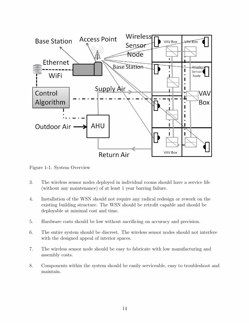
Figure 1-1. System Overview

3. The wireless sensor nodes deployed in individual rooms should have a service life(without any maintenance) of at least 1 year barring failure.

4. Installation of the WSN should not require any radical redesign or rework on theexisting building structure. The WSN should be retrofit capable and should bedeployable at minimal cost and time.

5. Hardware costs should be low without sacrificing on accuracy and precision.

6. The entire system should be discreet. The wireless sensor nodes should not interferewith the designed appeal of interior spaces.

7. The wireless sensor node should be easy to fabricate with low manufacturing andassembly costs.

8. Components within the system should be easily serviceable, easy to troubleshoot andmaintain.

14

1.3 Final System Layout

The WSN that is discussed in this thesis is shown in Figure 1-2. It has a star topology.

Individual nodes communicate to a central hub. Texas Instruments eZ430-RF2500 was

chosen to act as nodes and the hub in this WSN . The individual nodes are attached to

sensors and are called End Points (EP). The central hub is called an Access Point (AP).

The AP’s are connected to a plug computer or a base station using cables. Sensor data

from the EP’s are received at the AP. The base station logs the data onto a remotely hosted

database via the Internet. The control algorithms then access this data from the database.

Each EP has sensors that can measure temperature, humidity and CO2 levels. A Passive

Infrared (PIR) sensor included in the wireless sensor node detects motion. When there are

multiple occupants present in a room, the CO2 readings can be a measure of the occupancy.

Figure 1-2. Wireless Sensor Network

15

CHAPTER 2WIRELESS SENSOR NODE

The design and implementation of the wireless sensor node is discussed here. We went

through a complete product development cycle while designing the wireless sensor node.

The node needs to have sensors to monitor temperature, humidity, presence and carbon

dioxide as well as the ability to process and transmit sensor data to a base station. Thus

we will have to integrate all the sensors to a microprocessor for processing sensor data and

a radio for wireless communication. In the preliminary design phase, we look at various

options available for the hardware components and select the ones that meet our

requirements of cost and specifications. We then do a detailed design of the Printed Circuit

Board (PCB) and the packaging for the node. Finally, the software for the EP onboard the

wireless sensor node is discussed. Fabrication of the wireless sensor node is outsourced to a

local company due to the requirement of surface mount technology for soldering and the

large number of sensor nodes that have to be fabricated. Design of the node is constrained

by the need for easy assembly, dis assembly, hardware replacement and easy

troubleshooting.

2.1 Hardware Selection

Multiple choices were available for all the hardware components used in the wireless

sensor node. The best suited hardware was selected after careful consideration in terms of

cost and features.

2.1.1 Microprocessor and Radio

The first prototype was made using an Arduino Board, a Xbee transmitter and a Zilog

PIR sensor.

X-CTU software is used to interact with the Xbee modules. One of the modules was

set to receiving mode and is connected to a PC via a USB cable. The other Xbee module

which is a part of the prototype is set to transmit mode. The Xbee modules are configured

using the instructions given in [1].

16

Table 2-1. Comparison of Arduino+Zigbee and eZ430-Rf2500

Device Arduino + XBee eZ430-Rf2500Cost $85 $20Range 100 ft 15-30 ftMesh Networking Capability 4 5

Temperature Sensor 5 4

Low Power 5 4

Easy to program 4 5

Communication protocol Zigbee SimpliciTI

The Arduino board is programmed to read a digital value from the PIR sensor on one

of its I/O ports. The digital reading (1 corresponds to motion detected and 0 corresponds

to no motion detected) is sent to the Xbee wireless module set for transmission. The

receiving Xbee module receives the data and sends it to a computer via the serial port. It

was noted that the Xbee modules provided excellent range based on the hardware that was

being used. The Arduino platform is easy to program, has a very good online community

and has enough Analog/Digital ports for attaching peripherals/sensors. The only major

hindrance is the cost. The cost of the wireless module(XBEE) along with the

microcontroller(Arduino) is close to $85 per WSN.

Texas Instruments offers a complete wireless development tool - the eZ430-RF2500

(2-1) for $20 each. The eZ430-RF2500, includes a MSP430 microcontroller and a CC2500

radio along with the hardware required to develop an entire wireless project. It comes built

in with SimpliciTI, a proprietary low-power star network stack, which enables robust

wireless networks out of the box. The hardware includes the MSP430F22x4 which

combines 16-MIPS (million instructions per second) performance, a 10-bit

Analog-Digital-Converter (ADC) paired with a CC2500 multi-channel RF transceiver and

an integrated temperature sensor [11]. The only downside to this hardware platform is that

it has limited wireless range. Out of the box, it has a range of only 30 feet. This can be a

17

Figure 2-1. Texas Instruments eZ430-RF2500

major hindrance when the WSN is used in buildings with large floor areas. However, the

range can be extended by reducing the communication band width.

This Arduino based prototype established that it is possible to use wireless modules

coupled with micro controllers to transmit sensor data wirelessly however, the

eZ430-RF2500 was chosen to be the EP and AP in the WSN due to its low cost and ability

to meet all the other requirements including range.

2.1.2 Sensors

The eZ430-RF2500 platform supports analog and digital I/O. Sensors for sensing

humidity, CO2 and temperature commonly have analog outputs while PIR sensors usually

give a digital output. Sensors were selected to comply with the limitations of the

eZ430-RF2500 platform.

2.1.3 CO2 Sensor

Indoor CO2 levels are typically between 350 to 2500 ppm [7]. Commonly used CO2

sensors had errors ranging from 75 ppm to over 200 ppm [9]. Energy savings from DCV

based on occupancy depend on the accuracy of the CO2 sensors and so sacrificing accuracy

for lower hardware costs is not logical. The best choice for a CO2 sensor capable of

18

Table 2-2. Comparison of COZIR and K-30 Sensors

Sensor COZIR K-30Cost $175 $65Range 0-2000 ppm 0-10000 ppmPre-calibrated 4 4

Power consumption 3.5 mW 200 mWAccuracy ± 50 ppm ± 30 ppmWarm up time 3 Seconds 120 Seconds

measuring CO2 levels up to 2500 ppm at acceptable levels of accuracy was the Sensair K30

CO2 sensor. The K30 sensor has a measuring range of 0 to 10000 ppm at an accuracy of

±30 ppm. The accuracy of the K30 is better than most of the sensors tested in [9]. It

supports serial communication and has two selectable analog outputs. The only drawback

is that, the K30 is not suitable for low power applications as it operates on 150 mA at 5V.

Another option is a COZIR ultra low power CO2 sensor. It needs only 33 mA at 3.3V.

However, it can measure only up to 2000 ppm and is more expensive at $170 each at the

time of hardware selection. The K30 was selected as it gives better accuracy and range at

a low price of only $65 each. It comes pre-calibrated and does not need recalibration

during its lifetime. This is a major advantage as calibration drift of CO2 sensors has been

reported as a serious issue [9].

2.1.4 Humidity Sensor

A lot of humidity sensors are available commercially. Humidity sensors are based on

resistive, capacitative or thermal conductivity sensing technologies [16]. Capacitive sensors

are the most widely used because of their wide RH range and condensation tolerance. The

key features required in a humidity sensor for the wireless sensor node are: good accuracy,

wide range, ability to operate at less than 5V , analog or serial output. The HIH4030

humidity sensor from Honeywell satisfies all of the above and does not need any

calibration. Moreover, it comes as a surface mount device making it cheap and easy to use

on a Printed Circuit Board (PCB).

19

2.1.5 PIR Sensor

There are a lot of commercially available PIR sensors which are used for motion

detection. A PIR sensor measures infrared light emitted by objects in the environment in

its field of view. It gets triggered when an infrared source of intensity higher than the

background appears and then disappears, such as a human being moving in front of a wall.

The sensor detects this change in the heat signature of the environment. The Parallax PIR

sensor is capable of detecting motion at distances of up to 30ft. It can operate at 5V and

has an option to vary sensitivity if needed. The sensor also has an on board led which

lights up for visual feedback when motion is detected. Communication is through a digital

output. A compact form factor, good sensitivity and low price ($10 at the time of

development) makes the Parallax PIR sensor an ideal choice for the wireless sensor node.

2.1.6 Temperature Sensor

The EZ430 comes with a temperature sensor with a range of −10◦F to 500◦F . This is

more than sufficient for indoor climate monitoring. The temperature sensor is not accurate

and needs to be calibrated. Since most of the terminal VAV boxes have temperature

sensors, only a few rooms which do not have dedicated VAV boxes will need temperature

data from wireless sensor nodes.

2.2 Detailed Design

2.2.1 Prototype

The first prototype that integrated all the sensors to the eZ430-RF2500 was done on a

breadboard. All sensors were connected to their respective ports on the eZ430-RF2500.

The MSP430 was flashed with the code for the EP instructing it to read and transmit

sensor data. Power requirements for all peripherals on the node are not same. The

humidity sensor and the CO2 sensor operate at 5V while the eZ430-RF2500 and the PIR

sensor operate at 3.3V . An arduino board was used to supply the two voltages. The

prototype was tested after configuring an Access Point to receive sensor data transmitted

by the EP. After confirming that the eZ430-RF2500 was capable of reading sensor data and

20

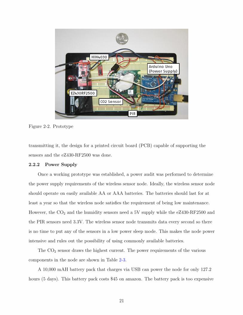
Figure 2-2. Prototype

transmitting it, the design for a printed circuit board (PCB) capable of supporting the

sensors and the eZ430-RF2500 was done.

2.2.2 Power Supply

Once a working prototype was established, a power audit was performed to determine

the power supply requirements of the wireless sensor node. Ideally, the wireless sensor node

should operate on easily available AA or AAA batteries. The batteries should last for at

least a year so that the wireless node satisfies the requirement of being low maintenance.

However, the CO2 and the humidity sensors need a 5V supply while the eZ430-RF2500 and

the PIR sensors need 3.3V. The wireless sensor node transmits data every second so there

is no time to put any of the sensors in a low power sleep mode. This makes the node power

intensive and rules out the possibility of using commonly available batteries.

The CO2 sensor draws the highest current. The power requirements of the various

components in the node are shown in Table 2-3.

A 10,000 mAH battery pack that charges via USB can power the node for only 127.2

hours (5 days). This battery pack costs $45 on amazon. The battery pack is too expensive

21

Table 2-3. Power requirements for various node components

Component Voltage (V) Current (mA)PIR Sensor 3.3 8.9Humidity Sensor 5 0.5CO2 5 40eZ430-RF2500 3.3 5.1

and the operating life constant for the node using such a battery pack is really low. Using

batteries for such a power intensive application is not possible and so the wireless sensor

node was designed to run on wall power. Power outlets are easily accessible in most

buildings.

One way of running the wireless sensor node off batteries is to operate it without the

CO2 sensor. This reduces the power requirement and the node can run for around 466

hours (20 days) on a 10,000 mAH battery. Hence the power jack on board the wireless

sensor node was chosen to be compatible with battery power packs for operating the node

temporarily in places without wall outlets.

2.2.3 PCB Design

A minimalistic approach was used to design the PCB board to keep the wireless sensor

node compact and light. The PCB was designed using proprietary software from Express

PCB. Express PCB is a low cost PCB manufacturer that has integrated PCB design and

ordering of PCB boards into a convenient software package. The PCB used for the wireless

sensor node is double sided. The design specifications for the board are:

1. 3.3V and 5V power supply

2. Programming headers for flashing the MSP430

3. Screw holes for fastening the PCB to the case

4. Pin holes for connecting CO2 , PIR and eZ430-RF2500

5. Surface mount slot for humidity sensor

A 5V wall adapter supplies power to the board. A power jack makes this power

available on the PCB. A 3.3V regulator is used to step down the voltage. The regulator

22

needs a 1µF capacitor at the input and a 10µF capacitor at the output. The output from

the regulator is wired to the eZ430-RF2500 and the PIR sensor. The CO2 sensor and the

humidity sensor are powered directly from the power jack. The pins on the eZ430-RF2500

that are used for flashing code on the MSP430 are also made available on the board . This

makes it easy to flash the MSP430 without removing it from the PCB. Since the CO2

sensor shares the pins on the eZ430-RF2500 used for programming, making it available

externally improves accessibility for troubleshooting the eZ430-RF2500. A schematic of the

PCB is shown in Figure 2-3.

Figure 2-3. Printed Circuit Board Schematic

2.2.4 Case Design

The PIR sensor on board the wireless sensor node needs direct line of sight to detect

motion. The node therefore should be positioned to have maximum visibility with the

occupant. As the node will be deployed in places such as office workstations, room walls

etc., it should appear pleasing. The packaging for the wireless sensor node was designed to

make it as discreet as possible. The material chosen for the casing is acrylonitrile butadiene

23

styrene (ABS). ABS is one of the most commonly used polymers for making electronic

packaging. It is strong, durable and light. To keep costs down, an existing mold from an

injection molding vendor was modified to meet our specifications. Ventilation holes all

around the periphery of the case ensure that the IAQ sensors have good access to the air

inside the room. The CAD drawing for the case used is shown in Figure 2-4. The case

fabricated as per the design in Figure 2-4 is shown in Figure 2-5.

Figure 2-4. Case-CAD Drawing

2.3 Software for the End Point

The EP is an eZ430-RF2500 programmed to read sensor data, process it, convert it

into hexadecimal and transmit it using the CC2500 radio. The EP acts as a node in a

wireless network with a star topology. The EP’s talk directly to the Access Points.

Communication is handled by the SimpliciTI network protocol. SimpliciTI is a low power

24

Figure 2-5. Case and Cover

radio-frequency (RF) protocol targeting simple small RF networks (< 100nodes). The

protocol runs out of the box on TI’s MSP430 microcontrollers. SimpliciTI supports only a

peer-to-peer network topology. However, hardware limitations limit the implementation of

mesh networks on the EZ430 platform and hence SimpliciTI ideal.

The eZ430-RF2500 is programmed using embedded C programming. Texas

Instruments Code Composer Studio (CCS) provides an Integrated Development

Environment(IDE) and the compiler for converting C code into binary. The flowchart for

the operations being performed at the EP is shown in Figure 2-6.

25

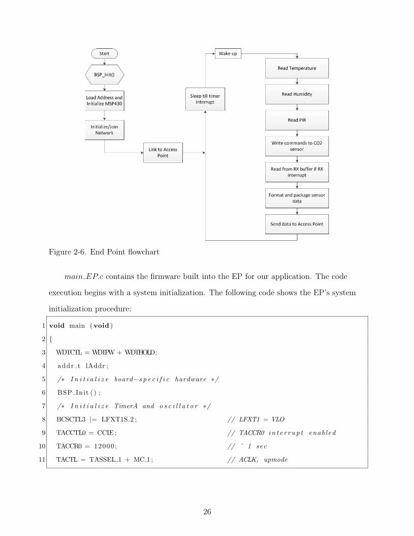
Figure 2-6. End Point flowchart

main EP.c contains the firmware built into the EP for our application. The code

execution begins with a system initialization. The following code shows the EP’s system

initialization procedure:

1 void main (void )

2 {

3 WDTCTL = WDTPW + WDTHOLD;

4 addr t lAddr ;

5 /∗ I n i t i a l i z e board−s p e c i f i c hardware ∗/

6 BSP Init ( ) ;

7 /∗ I n i t i a l i z e TimerA and o s c i l l a t o r ∗/

8 BCSCTL3 |= LFXT1S 2 ; // LFXT1 = VLO

9 TACCTL0 = CCIE ; // TACCR0 in t e r r u p t enab led

10 TACCR0 = 12000 ; // ˜ 1 sec

11 TACTL = TASSEL 1 + MC 1 ; // ACLK, upmode

26

BSP Init() SimpliciTI API call initializes the hardware on the eZ40-RF2500. It

establishes communication between the MSP430 and the CC2500 radio and initializes the

LEDs/switches on the board. The following other initializations are also performed:

• The DCO and MCLK are set to run at 8 MHz.

• Timer A is set to trigger interrupts at 1 second intervals.

• The universal serial communication interface (USCI) UART is initialized tocommunicate with the CO2 sensor.

After all the system components have been initialized, the EP tries to connect to an

AP that is listening for connections. The LED’s are turned on to indicate that joining is

yet to occur. The Timer A0 will wake the CPU up every second to try and establish a

connection. If a connection is made, both the LED’s are turned off. The following code

shows how the EP tries to establish a connection with a listening AP.

1 while (SMPL SUCCESS != SMPL Init (0 ) )

2 {

3 BSP TOGGLE LED1( ) ;

4 BSP TOGGLE LED2( ) ;

5 b i s SR r e g i s t e r ( LPM3 bits+GIE) ; // LPM3 with i n t e r r u p t s enab led

6 }

7 /∗ LEDs on s o l i d to i n d i c a t e s u c c e s s f u l j o i n . ∗/

8 BSP TURN OFF LED1( ) ;

9 BSP TURN OFF LED2( ) ;

10 /∗ Uncondi t iona l l i n k to AP which i s l i s t e n i n g due to s u c c e s s f u l j o i n . ∗/

11 l inkTo ( ) ;

If a successful connection is estabilshed, the protocol issues a handle called the LinkID.

This will be unique for each EP on the network just like an address. Individual packets

from each EP are identified at the AP using the LinkID. The linkTo() function handles

sensor data collection and communication once the EP has attained a working link to an

AP. TimerA0 wakes up the CPU every second to enable sensor data collection and

27

transmission. A flag - sSelfMeasureSem, inside the Timer interrupt routine keeps track of

whether sensor data needs to be measured or not.

Once the timer raises the sSelfMeasureSem flag, the sensor readings are attained

starting with the temperature sensor. The temperature sensor is mapped to one of the

ADC ports (Pin 2) on the eZ430-RF2500. A reference voltage of 1.5 V is used. The

reference is allowed to settle for at least 30µs before the analog port is sampled. The

measured value is then saved in an array. The following lines of code show how the

temperature is read via an analog port:

1 /∗ Get temperature ∗/

2 ADC10CTL1 = INCH 10 + ADC10DIV 4 ; // Temp Sensor ADC10CLK/5

3 ADC10CTL0 = SREF 1 + ADC10SHT 3 + REFON + ADC10ON + ADC10IE + ADC10SR;

4 /∗ Allow r e f v o l t a g e to s e t t l e f o r at l e a s t 30us (30 us ∗ 8MHz = 240

c y c l e s )

5 d e l a y c y c l e s (240) ;

6 ADC10CTL0 |= ENC + ADC10SC; // Sampling and convers ion s t a r t

7 b i s SR r e g i s t e r (CPUOFF + GIE) ; // LPM0 with i n t e r r u p t s enab led

8 r e s u l t s [ 0 ] = ADC10MEM; // Ret r i eve r e s u l t

9 ADC10CTL0 &= ˜ENC;

10

11 degC = (( ( temp − 673) ∗ 4230) / 1024) ; //

t emp ca l i b r a t i on

12 i f ( (∗ tempOffse t ) != 0xFFFF )

13 {

14 degC += (∗ tempOffse t ) ;

15 }

The analog value is converted into the required temperature value. Any errors in the

measurement are corrected using a one point calibration. The calibration constant is

represented as an offset and is different for different sensors. The calibration constant has

to be determined empirically. It is then updated on the code before the eZ430-RF2500 is

28

flashed. Assuming a zeroth order derivative, the temperature is calibrated as:

T̂ = TADC + offset (2–1)

The PIR sensor gives a digital o/p. An output high corresponds to motion detected.

The digital pin remains at output low if no motion is detected. One of the ADC pins (Pin

2.2) on the eZ430-RF2500 is set as a digital input. A value of 1 or 0 is assigned to a

variable based on the output at this pin. The following lines of code illustrate data

collection from a PIR sensor:

1 //Get PIR

2 int value ;

3 P2DIR &= ˜BIT2 ; // Set P2 .2 to input

4 value = (P2IN & BIT2) ;

The humidity sensor also gives an analog output. It is mapped to ADC Pin 8. It

requires a reference voltage of 2.5 V. The value measured is converted into the required

humidity value and is stored in a variable.

1 ADC10CTL0 = SREF 1 + ADC10SHT 3 + REFON + ADC10ON + ADC10IE + REF2 5V ;

2 d e l a y c y c l e s (240) ;

3 ADC10CTL0 |= REF2 5V ;

4

5 ADC10CTL1 = INCH 3 + ADC10DIV 3 ; // Input S e l c t and Clock Div

6 P2SEL = 0x08 ; // S e l e c t Pin 2.3

7 ADC10AE0 = 0x08 ; // ADC Low Bit (A3)

8 ADC10AE1 = 0x00 ;

9 ADC10CTL0 |= ENC + ADC10SC; // S ta r t to sample

10 b i s SR r e g i s t e r (CPUOFF + GIE) ; // LPM0 w/ in t

11 r e s u l t s [ 3 ] = ADC10MEM; // Store Resu l t

12 ADC10AE0 = 0 ; // Reset S e l e c t i o n Bi t s

13 ADC10AE1 = 0 ;

14 humidity = ( int ) ( ( ( ( ( ( r e s u l t s [ 3 ] / 1 0 2 3 . 0 ) ∗2 . 5 ) −.45) ∗100 .0 ) /3)−15) ;

//Derived from Datasheet In fo

29

Readings from the CO2 sensor are available in analog or serial format. During testing,

it was noted that the analog readings were not very reliable as the signal processing

algorithm built into the CO2 sensor works efficiently only when the data is read in serial

format. Polling the CO2 sensor via serial requires a free serial port on the eZ430-RF2500.

The eZ430-RF2500 has only one serial port which is used to flash the MCU. This port is

available once the MCU is flashed and can be used to read from the CO2 sensor. Polling

the CO2 sensor via the serial port involves sending a set of hexadecimal values to the

sensor. It then responds with the desired CO2 reading. The commands in 2-4 need to be

send to the CO2 sensor to initiate a response from the sensor [18].

After receiving the instruction list, the CO2 sensor measures the CO2 value and

transmits it via the serial port. The transmitted data will include the address of the CO2

sensor along with the measured CO2 levels. The measured value will be in hexadecimal

format with a high byte and a low byte. The response has the following format:

Table 2-4. Instruction set for CO2 sensor.

Address of the Sensor Read initiate commands0xFE 0x44 0x00 0x08 0x02 0x9F 0x25

The MSP430 MCU can read the response using an interrupt service routine [12]. The

following lines of code show how the interrupt service routine is implemented.

1 /∗ USCIA in t e r r u p t s e r v i c e rou t ine ∗/

2 #pragma vec to r=USCIAB0RX VECTOR

3 i n t e r r u p t void USCI0RX ISR(void )

4 {

5 i f (UCA0RXBUF == 0xFE) \\Check i f c o r r e c t data i s be ing sent

6 {

7 bufpos = 0 ;

8 bu f f e r [ bufpos ] = 0xFE ;

9 }

30

10 bu f f e r [ bufpos ] = UCA0RXBUF;

11 bufpos++;

12 }

The interrupt service routine gets activated when the CO2 sensor sends the first packet

of the response. Each packet gets stored in the RX buffer of the MSP430’s UART and is

transferred onto a temporary variable so that the more packets can be written into it. The

temporary variable, represents the response from the CO2 sensor.

Once all the sensor data is collected, it is converted into hexadecimal format made

ready for transmission. The following lines of code show how the sensor readings for

temperature, humidity and CO2 are formatted and stored in a temporary variable (msg).

1 //Temperature sensor

2 temp = r e s u l t s [ 1 ] ;

3 vo l t = ( temp∗25) /512 ;

4 msg [ 0 ] = degC&0xFF ;

5 msg [ 1 ] = (degC>>8)&0xFF ;

6 msg [ 2 ] = vo l t ;

7

8 //Humidity Sensor

9 msg [5 ]= humidity&0xFF ; // Package the humidi ty data in t o h igh and low

by t e s

10 msg [6 ]=( humidity>>8)&0xFF ;

11

12 //CO2 sensor

13 i f ( bu f f e r [0]==0xFE)

14 {

15 msg [3 ]= bu f f e r [ 3 ] ;

16 msg [4 ]= bu f f e r [ 4 ] ;

17 }

31

The temporary variable is sent to the access point using the SMPL SendOpt

SimpliciTI API. The LinkID for the EP assigned by the network is sent along with the

transmitted message.

32

CHAPTER 3ACCESS POINT

3.1 Hardware

The Access Point is a ez430-RF2500 board that relays data between the end point and

the base station. The AP interfaces with the base station over USB as a serial device. A

USB to serial converter configured to operate at 3.3V VCC and 3.3V I/O enables serial

communication. The COM port settings are 9600, N, 8, 1 (baud, parity, data bits, stop

bits).

3.2 Software

The AP acts as a data hub in a wireless network with a star topology. All the End

Points act as nodes and talk directly to the AP. Communication is handled by the

SimpliciTI network protocol. The sequence of operation of the AP is shown in Figure 3-1.

Figure 3-1. Access Point flowchart

33

main AP.c contains the firmware built into the AP for our application. The code

execution begins with a system initialization that is almost identical to the EP’s in the

network. The following code shows the AP’s system initialization procedure:

1 void main (void )

2 {

3 b sp IS t a t e t i n tS t a t e ;

4 /∗ I n i t i a l i z e board ∗/

5 BSP Init ( ) ;

6

7 /∗ I n i t i a l i z e TimerA and o s c i l l a t o r Reference : G l i t o v s k y ∗/

8 BCSCTL3 |= LFXT1S 2 ; // LFXT1 = VLO

9 TACCTL0 = CCIE ; // TACCR0 in t e r r u p t enab led

10 TACCR0 = 12000 ; // ˜1 second

11 TACTL = TASSEL 1 + MC 1 ; // ACLK, upmode

12

13 /∗ I n i t i a l i z e s e r i a l por t ∗/

14 COM Init ( ) ;

BSP Init() SimpliciTI API call initializes the hardware on the EZ40. This call

initializes the communication between the MSP430 and the CC2500 radio and the

LEDs/switches on the board. The following other initializations are also performed:

• The DCO and MCLK are set to run at 8 MHz.

• Timer A is set to trigger interrupts at 1 second intervals.

• The universal serial communication interface (USCI) UART is initialized tocommunicate with the PC Com port.

Once hardware initialization is complete, the SMPL Init(sCB) function, initializes

the network. The sCB parameter is a function pointer that is executed within the interrupt

service routine (ISR) upon packet reception by the AP. Once network initialization is

complete, both the LEDs are turned on to indicate that the AP is waiting for an EP to join.

34

The sCB call back function, filters the received packet according to its link ID to

identify the source of transmission and distinguish the EP join request from a data packet

transmission from an EP that has already established a connection to the network. A link

ID of 0 identifies a join request. Upon acceptance of an EP join request, the AP

enumerates new members to the network and assigns incremental IDs from 0x01 to 0x1D.

The possible enumeration values from 0x01 to 0x1D are a design network constraint for the

SimpliciTI protocol that allows up to 30 devices to be linked to the AP. A link ID from

0x01 to 0x1D identifies the reception of a packet from one of the network EP’s. For our

application, the maximum number of connections is restricted to 8.

According to the link ID, the sCB callback function identifies and increments the

respective sPeerFrameSem[aphore] or sJoinSem[aphore] for handling the program’s main

loop. These two semaphores, control the program flow after network initialization.

3.2.1 sJoinSem Branch

The sJoinSem semaphore is set when an EP calls its SMPL Init() function. A join to

the network is actually a side effect of initialization, as there is never an actual call made

that requests a network join. When the sJoinSem[aphore] has been set in the AP’s callback

function and as long as the AP has made less than its maximum number of links, the AP

will call its SMPL LinkListen() function. As the function parameter, the link listen

function, takes a pointer to the link ID that will be used to communicate with the linked

EP. SMPL LinkListen() is a blocking call, meaning it will not return until a successful

link has been created, so it is important that the SMPL LinkListen() call be made only

when the user knows that another device has made the link request using the

SMPL Link(). On a successful link creation, the sJoinSem branch increases the number of

devices that the AP recognizes as part of the network and unlocks the sJoinSem[aphore] for

another device to set. Implementation of the sJoinSem branch is shown in the following

lines of code:

1

35

2 i f ( sJoinSem && ( sNumCurrentPeers < NUMCONNECTIONS) )

3 {

4 /∗ l i s t e n f o r a new connect ion ∗/

5 while (1 )

6 {

7 i f (SMPL SUCCESS == SMPL LinkListen(&sLID [ sNumCurrentPeers ] ) )

8 {

9 break ;

10 }

11

12 }

13

14 sNumCurrentPeers++;

15

16 BSP ENTER CRITICAL SECTION( in tS t a t e ) ;

17 sJoinSem−−;

18 BSP EXIT CRITICAL SECTION( in tS t a t e ) ;

19 }

3.2.2 sPeerFrameSem Branch

The sPeerFrameSem semaphore is incremented in the callback function every time the

AP receives a frame from a EP. In the case that the sPeerFrame Sem[aphore] has been set

or incremented, the AP first defines a message buffer in which to store the current frame

being analyzed and then loop through its input queue searching for messages until it has

processed all of the waiting frames. The following lines of code shows how the EP messages

are handled.

1 i f ( sPeerFrameSem )

2 {

3 u i n t 8 t msg [ 1 0 ] , len , i ;

4

5 /∗ process a l l frames wa i t ing ∗/

36

6 for ( i =0; i<sNumCurrentPeers ; ++i )

7 {

8 i f (SMPL SUCCESS == SMPL Receive ( sLID [ i ] , msg , &len ) )

9 {

10 i o c t lR ad i o S i g i n f o t s i g I n f o ;

11

12 processMessage ( sLID [ i ] , msg , l en ) ;

13

14 s i g I n f o . l i d = sLID [ i ] ;

15

16 SMPL Ioctl (IOCTL OBJ RADIO, IOCTL ACT RADIO SIGINFO, (void ∗)&

s i g I n f o ) ;

17 //TXString ( ( char ∗)msg , l en ) ;

18 transmitData ( i , s i g I n f o . s i g I n f o . r s s i , (char∗)msg ) ;

19

20 BSP TOGGLE LED2( ) ;

21

22 BSP ENTER CRITICAL SECTION( in tS t a t e ) ;

23 sPeerFrameSem−−;

24 BSP EXIT CRITICAL SECTION( in tS t a t e ) ;

25 }

26 }

3.2.3 Writing to the Serial Port

Functions to handle communication through the serial port are defined in

virtual com cmds.c. The pins to handle serial port communication are initialized first.

P3.4 is chosen as TX and P3.5 is chosen as RX. The universal serial communication

interface (USCI) is then initialized along with the RX interrupt.

Message packets from the EP’s in hexadecimal format are passed as arguments to the

function transmitDataString. This function, converts the hexadecimal values to decimal

and then formats it into a string. The formatted string is written into the serial buffer by

37

the function TXString. This function uses pointers to fill the TX buffer. The following

lines of code show the implementation of TXString:

1 void TXString ( char∗ s t r i ng , int l ength )

2 {

3 int po in t e r ;

4 for ( po in t e r = 0 ; po in t e r < l ength ; po in t e r++)

5 {

6 volat i le int i ;

7 while ( ! ( IFG2&UCA0TXIFG) ) ; // USCI A0 TX bu f f e r ready?

8 UCA0TXBUF = s t r i n g [ po in t e r ] ;

9 }

10 }

A check is performed at each iteration to ensure that the TX buffer is ready and to

avoid overwriting of the buffer. The formatted string being written into the serial port is as

follows:

1 [ 0 0 ] $1010 , 7 2 . 7F,0608ppm,040 ,0 no \\ address , temperature , CO2 l e v e l , humidity ,

occupancy

2 [ 0 0 ] $1004 , 7 2 . 9F,0611ppm,041 ,0 no

3 [ 0 0 ] $1006 , 7 1 . 8F,0621ppm,039 ,0 no

4 [ 0 0 ] $1012 , 7 0 . 5F,0599ppm,040 ,0 no

5 [ 0 0 ] $1005 , 7 2 . 4F,0601ppm,041 ,0 no

6 [ 0 0 ] $1007 , 7 3 . 6F,0615ppm,040 ,0 no

38

CHAPTER 4TESTING AND VALIDATION

The wireless nodes were manufactured as per the design presented in Section 2. The

design and the peripherals sourced from various vendors were provided to Just In Time

Manufacturing - a contract manufacturing company. The first batch of 5 nodes was

fabricated to establish the manufacturing cost and to obtain samples for testing. The

difficulties in manufacturing the box were noted and the design was tweaked to remove

these. A total of 70 nodes were fabricated with the new updated design. The finished

wireless sensor node when deployed on a wall is shown in Figure 4-1.

Figure 4-1. Wireless Sensor Node - Deployed on a wall

For testing the WSN we need a base station that can log data from the AP onto a

database. Section 4.1 details the base station that was used for testing the WSN .

39

4.1 Base Station

The main role of the base station is to receive data from the AP, time stamp it and

write the data to a remotely hosted database via the Internet. For this purpose we need a

plug computer capable of running a script that can read data from the serial port, process

it and write it to a database. The Dream plug from Marvell is a compact plug computer

that is capable of running Debian Linux. It comes preloaded with the operating system. It

has 802.11b/g WiFi adapter, two Ethernet port, two USB ports and 4 GB of internal

memory. Thanks to its ruggedness and compact form factor it can be concealed when

deployed in buildings. The Dream plug is chosen as the base station.

A FTDI serial to USB converter that has a 3.3V serial I/O and a 3.3V power supply is

used to connect the AP to the base station. A python script is executed on the base

station to log data coming in from the AP. The python script starts with initialization.

The database connection and serial communication with the AP are established. The

following lines of code written by Siddarth Goyal illustrate the initialization process.

1

2 db = po s t g r e s q l . open ( ”pq :// po s tg r e s : therock@10 . 2 45 . 1 6 . 2 27/ po s tg r e s ” ) \\

Database connect ion opened

3 por t s=[”/dev/ttyUSB0” , ”/dev/ttyUSB1” , ”/dev/ttyUSB2” , ”/dev/ttyUSB3” ] \\

Ports to check for connect i ons

4 #por t s=[”/dev/ttyUSB0” , ”/dev/ttyUSB2” ]

5 \\ s e r i a l port s e t t i n g s

6 by t e s i z e=8

7 ra t e=9600

8 pa r i t y=0

9 s t opb i t=1

10 debug=True

The pyserial API is used to handle serial communication. Each line represents data

from one of the EP’s. The line.decode function is used to process each data set. The sensor

40

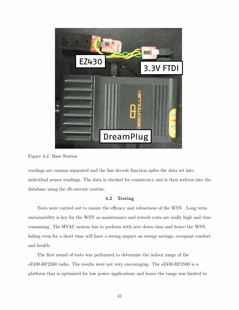
Figure 4-2. Base Station

readings are comma separated and the line.decode function splits the data set into

individual sensor readings. The data is checked for consistency and is then written into the

database using the db.execute routine.

4.2 Testing

Tests were carried out to ensure the efficacy and robustness of the WSN . Long term

sustainability is key for the WSN as maintenance and rework costs are really high and time

consuming. The HVAC system has to perform with zero down time and hence the WSN

failing even for a short time will have a strong impact on energy savings, occupant comfort

and health.

The first round of tests was performed to determine the indoor range of the

eZ430-RF2500 radio. The results were not very encouraging. The eZ430-RF2500 is a

platform that is optimized for low power applications and hence the range was limited to

41

less than 15 feet. This was not acceptable as base stations are expensive and hence

deployment costs will not be justifiable.

A significant improvement in range can be attained by decreasing the data rate. The

SimpliciTI protocol has a data rate of 250 kbps by default. Such a high data rate is not

required for our application as each data packet being transmitted by the EP’s is less than

1.6 KB and the sensor data is being transmitted once every second. A data rate of 2 kbps

will be sufficient. The data rate for the communication channel is determined by

parameters set in mrfi defs.h within the SimpliciTI protocol. The modified definitions are

shown below:

1

2 #define mrfi LENGTH FIELD SIZE 1

3 #define mrfi ADDR SIZE 4

4 #define mrfi MAX PAYLOAD SIZE 20

5

6 #define mrfi RX METRICS SIZE 2

7 #define mrfi RX METRICS RSSI OFS 0

8 #define mrfi RX METRICS CRC LQI OFS 1

9 #define mrfi RX METRICS CRC OK MASK 0x80

10 #define mrfi RX METRICS LQI MASK 0x7F

11

12 #define mrfi NUM LOGICAL CHANS 4

13 #define mrfi NUM POWER SETTINGS 3

14

15 #define mrfi BACKOFF PERIOD USECS 250

16

17 #define mrfi LENGTH FIELD OFS 0

18 #define mrfi DST ADDR OFS ( mrfi LENGTH FIELD OFS +

mrfi LENGTH FIELD SIZE )

19 #define mrfi SRC ADDR OFS ( mrfi DST ADDR OFS +

mrfi ADDR SIZE )

42

20 #define mrfi PAYLOAD OFS ( mrfi SRC ADDR OFS +

mrfi ADDR SIZE )

21

22 #define mrfi HEADER SIZE (2 ∗ mrfi ADDR SIZE )

23 #define mrfi FRAME OVERHEAD SIZE ( mrfi LENGTH FIELD SIZE +

mrfi HEADER SIZE )

24

25 #define mrfi GET PAYLOAD LEN (p) ( ( p)−>frame [ mrfi LENGTH FIELD OFS ]

− mrfi HEADER SIZE )

26 #define mrfi SET PAYLOAD LEN (p , x ) s t ( (p)−>frame [

mrfi LENGTH FIELD OFS ] = x + mrfi HEADER SIZE ; )

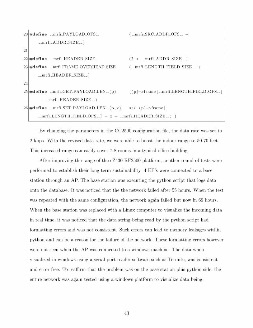
By changing the parameters in the CC2500 configuration file, the data rate was set to

2 kbps. With the revised data rate, we were able to boost the indoor range to 50-70 feet.

This increased range can easily cover 7-8 rooms in a typical office building.

After improving the range of the eZ430-RF2500 platform, another round of tests were

performed to establish their long term sustainability. 4 EP’s were connected to a base

station through an AP. The base station was executing the python script that logs data

onto the database. It was noticed that the the network failed after 55 hours. When the test

was repeated with the same configuration, the network again failed but now in 69 hours.

When the base station was replaced with a Linux computer to visualize the incoming data

in real time, it was noticed that the data string being read by the python script had

formatting errors and was not consistent. Such errors can lead to memory leakages within

python and can be a reason for the failure of the network. These formatting errors however

were not seen when the AP was connected to a windows machine. The data when

visualized in windows using a serial port reader software such as Termite, was consistent

and error free. To reaffirm that the problem was on the base station plus python side, the

entire network was again tested using a windows platform to visualize data being

43

transmitted by the AP. The network however, failed again in almost the same time (51

hours). We can now safely assume that the reason for failure is at the AP or base station.

Changes to the format in which the AP transmits data did not solve the issue. The

AP employs a timer that is used to read the temperature sensor on board the

eZ430-RF2500. There is another timer that takes care of receiving wireless data and

communication through the serial port. A hypothesis was that the presence of two timers

(one is dependent on the other) may be leading to memory issues on the resource limited

eZ430-RF2500 platform. The eZ430-RF2500 acting as the AP does not need to sense

temperature. The only function of the AP is to receive wireless data and to forward it to

the serial port. We can safely disable the timer that controls the temperature reading and

reporting on the AP without any significant impact on the WSN . The AP now has only

one timer that takes care of receiving and forwarding wireless data.

Another hypothesis was that the python script was resetting the AP as both the AP

and the base station shared the same serial buffer. It was proposed that the API used to

read from the serial port in python was causing memory issues. As the AP wrote data into

this buffer, memory overflow on the serial buffer can stifle the AP from writing to the same

buffer. To rectify this issue, the python code was made to reset every 24 hours.

The WSN was again tested using the single timer AP connected to a base station

running a self resetting python script. The WSN worked without any hiccups for 30 days.

This test establishes the long term viability of the WSN .

Each AP on the WSN can connect to a maximum of 8 EP’s. The number 8 is limited

by the SimpliciTI protocol due to the eZ430-RF2500 platforms limited hardware. This

limitation can be a major hindrance if there is a need to scale the the network. We face

this challenge as we plan to deploy and test a 70 node network in a building at the

University of Florida campus. Atleast 8 AP’s will be needed to service this building. To

limit interference and to ensure that the EP’s communicate only with the AP to which it

has been assigned, the AP’s were set to operate at different frequency channels. The base

44

frequency used is 2424.998 MHz. Each channel is spaced 249.938 MHz apart. EP’s set to

operate on channel 1 can only communicate with the AP that is listening on channel 1.

The network can thus be easily scaled with limited interference.

4.3 Deployment

The wireless sensor network will be used to implement an advanced control algorithm

on the HVAC system at a building (Pugh Hall) on the University of Florida campus. 70

wireless sensor nodes will be connected to 10 base stations to cover the entire floor area of

the building. A schematic of the location of the base stations and the wireless sensor nodes

on Floor 2 of the building is shown in Figure 4-3.

4.4 Cost Analysis

The cost of deploying and operating a wireless network for HVAC control should be

minimal as most HVAC designers have limited funds for retrofits. Also an investment to

reduce energy costs should have payback periods of 3 years or less. The entire design of the

WSN was performed keeping hardware costs to a minimum. The design of the wireless

sensor node and the network was done by graduate students earning $20 an hour. The

design and development of the nodes took 12 weeks. The fabrication of the nodes is

outsourced to a local company which charges $76.68 each for soldering and assembling all

the components within the node. Testing and validation of the WSN required 15 weeks

taking the development time to a total of 27 weeks. A graduate student typically dedicates

half of his 20 hour week to research and so over a 27 week period, at least 270 hours would

have been spent on developing the WSN . The labor cost for R&D will thus be close to

$5400. Considering only the cost of hardware and fabrication, each node costs $214.90.

The component wise price break up is shown in Table 4-1. Prices can be further reduced

for large quantities by optimizing the manufacturing setup and obtaining bulk quantity

discounts on the components.

45

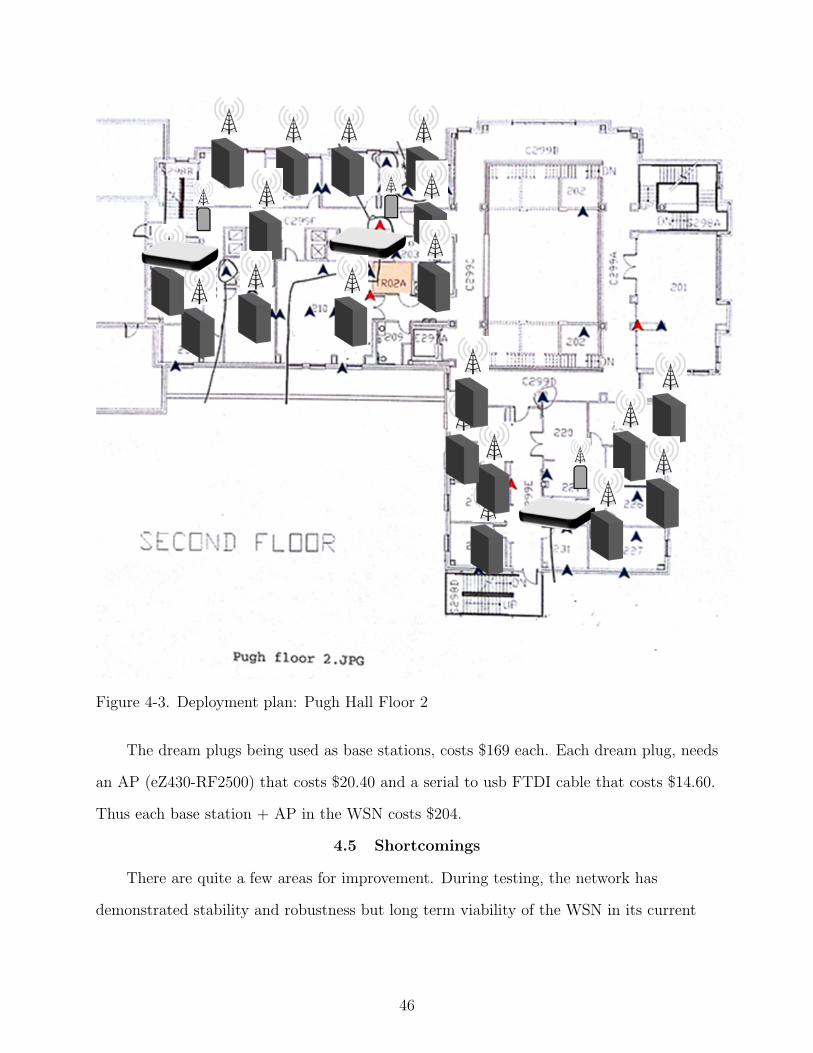
Figure 4-3. Deployment plan: Pugh Hall Floor 2

The dream plugs being used as base stations, costs $169 each. Each dream plug, needs

an AP (eZ430-RF2500) that costs $20.40 and a serial to usb FTDI cable that costs $14.60.

Thus each base station + AP in the WSN costs $204.

4.5 Shortcomings

There are quite a few areas for improvement. During testing, the network has

demonstrated stability and robustness but long term viability of the WSN in its current

46

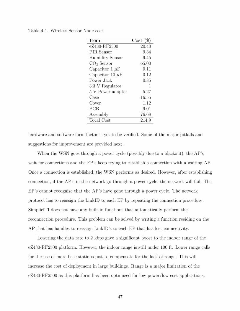
Table 4-1. Wireless Sensor Node cost

Item Cost ($)eZ430-RF2500 20.40PIR Sensor 9.34Humidity Sensor 9.45CO2 Sensor 65.00Capacitor 1 µF 0.11Capacitor 10 µF 0.12Power Jack 0.853.3 V Regulator 15 V Power adapter 5.27Case 16.55Cover 1.12PCB 9.01Assembly 76.68Total Cost 214.9

hardware and software form factor is yet to be verified. Some of the major pitfalls and

suggestions for improvement are provided next.

When the WSN goes through a power cycle (possibly due to a blackout), the AP’s

wait for connections and the EP’s keep trying to establish a connection with a waiting AP.

Once a connection is established, the WSN performs as desired. However, after establishing

connection, if the AP’s in the network go through a power cycle, the network will fail. The

EP’s cannot recognize that the AP’s have gone through a power cycle. The network

protocol has to reassign the LinkID to each EP by repeating the connection procedure.

SimpliciTI does not have any built in functions that automatically perform the

reconnection procedure. This problem can be solved by writing a function residing on the

AP that has handles to reassign LinkID’s to each EP that has lost connectivity.

Lowering the data rate to 2 kbps gave a significant boost to the indoor range of the

eZ430-RF2500 platform. However, the indoor range is still under 100 ft. Lower range calls

for the use of more base stations just to compensate for the lack of range. This will

increase the cost of deployment in large buildings. Range is a major limitation of the

eZ430-RF2500 as this platform has been optimized for low power/low cost applications.

47

Using other radios instead of the CC2500 can result in a significant boost in range. Xbee

radios running on the Zigbee protocol are available commercially with a range of up to 10

km. However, they will increase the cost of each wireless sensor node by $65.

Hardware limitations of the eZ430-RF2500 prevent the implementation of mesh

networks. Also they are not capable of running embedded operation systems such as Tiny

OS. As a result, the microprocessor on board cannot be programmed over the air. They

have to be brought back to the lab to be re programmed. Doing firmware upgrades in a

large building where a lot of wireless sensor nodes have been deployed is a laborious task in

the current configuration of the WSN .

Although using wall power is reliable and cheap, wall sockets are not always

available/accessible in all rooms. By optimizing the hardware to consume very little power,

we can run the wireless sensor node off readily available low cost batteries. Low power

devices are usually more expensive and less efficient. For example an ultra low power CO2

sensor, costs $175 while the one used in the wireless sensor node costs only $65.

The EP’s in the network are assigned LinkIDs by the SimpliciTI protocol. All the AP’s

the vicinity of the network which assigned the ID can communicate with the EP’s. There is

no way for an EP to decide which AP it wants to connect to. This restriction makes it

difficult to prevent the EP’s from communicating with two nearby base stations. As each

AP can connect to only 8 EP’s, we wish to keep multiple connections at a minimum.

48

CHAPTER 5CONCLUSION AND FUTURE WORK

5.1 Summary

In this thesis, we have shown the development cycle of a Wireless Sensor Network for

collecting climate, occupancy and IAQ data from within buildings. This data will then be

used by advanced control algorithms to optimize the operation of VAV terminal reheat

based HVAC systems. The WSN consists of wireless sensor nodes with End Points that

rely data to Access Points that are connected to base stations. Base stations, log the data

into a database via Ethernet or WiFi. The WSN was tested to ensure that it meets all of

the system requirements. Tests were conducted to establish its long term sustainability and

robustness.

5.2 Future Work

The WSN will be deployed and tested at Pugh Hall, a 40,000 sq ft LEED certified

building on the University of Florida campus. The building has a VAV terminal reheat

HVAC system and is ideal for testing the functionality of the WSN .

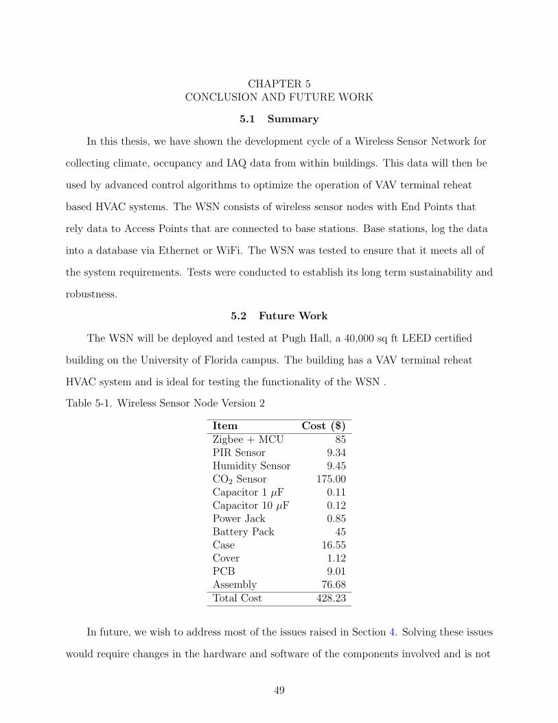
Table 5-1. Wireless Sensor Node Version 2

Item Cost ($)Zigbee + MCU 85PIR Sensor 9.34Humidity Sensor 9.45CO2 Sensor 175.00Capacitor 1 µF 0.11Capacitor 10 µF 0.12Power Jack 0.85Battery Pack 45Case 16.55Cover 1.12PCB 9.01Assembly 76.68Total Cost 428.23

In future, we wish to address most of the issues raised in Section 4. Solving these issues

would require changes in the hardware and software of the components involved and is not

49

trivial. The cost of components for an updated wireless sensor node is shown in Table 5-1.

The low power CO2 sensor will enable the wireless sensor node to last up to 8 months on a

10,000 mAH battery pack. This is a significant improvement over the current hardware.

The new wireless sensor node will allow more than 8 connections for each AP. The

range of each AP will also increase substantially as Zigbee radios have indoor range of up

to 500ft. This translates to fewer number of base stations in each WSN . Cost of each base

station can also be reduced by using a Raspberry PI instead of dream plug. A Raspberry

PI is a low cost plug computer and satisfies all the requirements for a base station. A

Raspberry PI costs only $25.

50

REFERENCES

[1] U. S. G. Energy Use Administration, “Electricity explained - use of electricity,” 2010.[Online]. Available:http://www.eia.gov/energyexplained/index.cfm?page=electricity use

[2] M. J. Brandemuehl and J. E. Braun, “The impact of demand-controlled andeconomizer ventilation strategies on energy use in buildings,” ASHRAE Transactions,vol. 105, 1999.

[3] V. Erickson, M. A. Carreira-Perpinan, and A. Cerpa, “OBSERVE: Occupancy-basedsystem for efficient reduction of HVAC energy,” in 10th International Conference onInformation Processing in Sensor Networks (IPSN 2010), April 2011, pp. 258–269.

[4] S. Goyal, H. Ingley, and P. Barooah, “Zone-level control algorithms based onoccupancy information for energy efficient buildings,” in American Control Conference(ACC), 2012, pp. 3063–3068.

[5] M. Morari, F. Oldewurtel, and D. Sturzenegger, “Importance of OccupancyInformation for Building Climate Control,” Applied Energy, Jan. 2012. [Online].Available:http://control.ee.ethz.ch/index.cgi?page=publications;action=details;id=3984

[6] F. Oldewurtel, D. Gyalistras, M. Gwerder, C. Jones, A. Parisio, V. Stauch,B. Lehmann, and M. Morari, “Increasing Energy Efficiency in Building ClimateControl using Weather Forecasts and Model Predictive Control,” in Clima - RHEVAWorld Congress, Antalya, Turkey, May 2010.

[7] American Society of Heating, Refrigerating and Air-Conditioning Engineers, Inc.,“ANSI/ASHRAE standard 62.1-2007, ventilation for acceptable air quality,” 2007.[Online]. Available: www.ashrae.org

[8] J. R. Sand, “Demand-controled ventilation using co2 sensors,” U.S. Department ofEnergy, Energy Efficiency and Renewable Energy, Tech. Rep., March 2004.

[9] N. Nassif and M. Zaheer-Uddin, “Simulated performance analysis of a multizone VAVsystem under different ventilation control strategies,” ASHRAE Transactions, pp.617–629, Jan 2007.

[10] S. J. Emmerich and A. K. Persily, “State-of-the-art review of CO2 demand controlledventilation technology and application, NISTIR 6729,” National Institute of Standardsand Technology, Tech. Rep., July 2001.

[11] R. Subramany, C. Liao, and P. Barooah, “Performance comparison of sensing systemsfor building occupancy measurement,” Energy and Buildings, 2012.

[12] R. American Society of Heating and I. Air-Conditioning Engineers, “Ansi/ashraestandard 55-1981, thermal environmental conditions for human occupancy,” 1992.[Online]. Available: www.ashrae.org

51

[13] A. TenWolde and W. B. Rose, “Criteria for humidity in the building and the buildingenvelope,” in Proceedings of workshop on control of humidity for health,artifacts andbuildings, November 1993, pp. 63–65.

[14] “Arduino instructions.” [Online]. Available: http://www.ladyada.net/learn/arduino/

[15] T. Instruments, “ez430-rf2500 user’s guide,” 2007. [Online]. Available:www.ti.com/lit/ug/slau227e/slau227e.pdf

[16] C. Erdmann, K. Steiner, and M. Apte, “Indoor carbondioxide concentrations andsickbuilding syndrome symptoms in the base study revisitted: Analysis of 100 bulidigdataset,” in Proceedings: Indoor Air 2012.

[17] W. Frisk, D. Sullivan, D. Faulkner, and E.Eliseeva, “Co2 monitoring for demandcontrol ventilation in commercial buildings,” California Energy commisssion report,2011.

[18] D. K. Roveti, “Choosing a humidity sensor: A review of three technologies,” July2001. [Online]. Available: http://www.ohmicinstruments.com/home/?p=179

[19] Sensair, “K-30 CO2 sensor communication documentation.” [Online]. Available:http://co2meters.com/Documentation/Other/SenseAirCommGuide.zip

[20] G. Litovsky, “Beginning microcontrollers with the msp430 - tutorial.” [Online].Available: http://www.glitovsky.com/Tutorialv0 4.pdf

52

BIOGRAPHICAL SKETCH

Rahul will begin his career in June 2013, as a Senior Mechanical Engineer with Lutron

Electronics in West Palm Beach, where he will be a member of the new product

development team. He shares the company’s passion and dedication to design and build

innovative products that can enrich lives without affecting mother nature.

Rahul will graduate with a Master of Science degree in mechanical engineering from

the University of Florida, Gainesville in May 2013. Since October 2011, he has been a

Graduate Research Assistant in the Distributed Control Systems Lab at the University of

Florida under Dr. Prabir Barooah. His research is focused on developing solutions for the

control of Heating and Air Conditioning Systems in smart buildings.

During his master’s program he has been a Teaching Assistant for multiple courses.

He has also done research in data acquisition using quadcopters and condition monitoring

of machine tools.

Rahul earned his Bachelor of Technology degree in mechanical engineering from

Amrita Vishwavidyapeetham in 2011. He interned at Bharat Heavy Electricals Limited

and Toyota Kirloskar Auto Parts while pursuing his degree. His undergraduate dissertation

entitled, Condition monitoring of end mill cutter using Artificial Intelligence was

supervised by Dr. Babudevasenapati.

53