c© 2012 Andreas Stefan Manfred Hagemann

THREE ESSAYS IN ECONOMETRICS

BY

ANDREAS STEFAN MANFRED HAGEMANN

DISSERTATION

Submitted in partial fulfillment of the requirementsfor the degree of Doctor of Philosophy in Economics

in the Graduate College of theUniversity of Illinois at Urbana-Champaign, 2012

Urbana, Illinois

Doctoral Committee:

Professor Roger Koenker, ChairProfessor Xiaofeng ShaoProfessor Daniel P. McMillenProfessor Anil K. Bera

ABSTRACT

This dissertation consists of three essays. In the first essay, entitled “Robust

Spectral Analysis,” I introduce quantile spectral densities that summarize

the cyclical behavior of time series across their whole distribution by analyz-

ing periodicities in quantile crossings. This approach can capture systematic

changes in the impact of cycles on the distribution of a time series and allows

robust spectral estimation and inference in situations where the dependence

structure is not accurately captured by the auto-covariance function. I study

the statistical properties of quantile spectral estimators in a large class of

nonlinear time series models and discuss inference both at fixed and across

all frequencies. Monte Carlo experiments and an empirical example illustrate

the advantages of quantile spectral analysis over classical methods when stan-

dard assumptions are violated.

In the second essay, “Stochastic Equicontinuity in Nonlinear Time Series

Models,” I provide simple and easily verifiable conditions under which a

strong form of stochastic equicontinuity holds in a wide variety of modern

time series models. In contrast to most results currently available in the

literature, my methods avoid mixing conditions. I discuss two applications

in detail.

In the third essay, “A Simple Test for Regression Specification with Non-

Nested Alternatives,” I introduce a simple test for the presence of the data-

generating process among several non-nested alternatives. The test is an

extension of the classical J test for non-nested regression models. I also

provide a bootstrap version of the test that avoids possible size distortions

inherited from the J test.

ii

Fur meine Eltern

iii

ACKNOWLEDGMENTS

I will always be indebted to my thesis advisor Roger Koenker for his guidance,

insight, and patience. Working with him has been a constant source of

inspiration and motivation for me. Xiaofeng Shao taught me a lot about

econometrics and statistics, and I benefited enormously from his comments

on the first chapter of my dissertation. Dan Bernhardt tirelessly read through

several drafts of my manuscripts and provided advice and criticism that

helped me improve the presentation of my work. I also received helpful

comments from Anil Bera, Dan McMillen, Jiaying Gu, Euler Mello, Tom

Parker, and seminar participants at the University of Illinois.

Before coming to the University of Illinois, I was fortunate enough to meet

Gabriel Lee and Rolf Tschernig at the Universitat Regensburg. Gabe con-

vinced me to go to graduate school, which I still think is one of the best

decisions I have ever made. I wish to thank him for all of his advice over the

years. Rolf encouraged me to pursue econometrics and gave me important

early feedback on my projects. I am grateful for his continuing interest in

my work. I would also like to thank Harry Haupt at the Universitat Bielefeld

for his help in getting me into graduate school.

Finally, my most heartfelt thanks to Sarah Miller and my parents for all

the love and support they have given me throughout these years. This dis-

sertation is dedicated to my parents.

iv

TABLE OF CONTENTS

CHAPTER 1 ROBUST SPECTRAL ANALYSIS . . . . . . . . . . . 11.1 Introduction . . . . . . . . . . . . . . . . . . . . . . . . . . . . 11.2 Quantile Spectra and Two Estimators . . . . . . . . . . . . . . 41.3 Asymptotic Properties of Quantile and Smoothed Quantile

Periodograms . . . . . . . . . . . . . . . . . . . . . . . . . . . 91.4 Testing for Flatness of a Quantile Spectrum . . . . . . . . . . 171.5 Numerical Results . . . . . . . . . . . . . . . . . . . . . . . . . 221.6 Conclusion . . . . . . . . . . . . . . . . . . . . . . . . . . . . . 391.7 Proofs . . . . . . . . . . . . . . . . . . . . . . . . . . . . . . . 39

CHAPTER 2 STOCHASTIC EQUICONTINUITY IN NONLIN-EAR TIME SERIES MODELS . . . . . . . . . . . . . . . . . . . . 552.1 Introduction . . . . . . . . . . . . . . . . . . . . . . . . . . . . 552.2 Stochastic Equicontinuity in Nonlinear Time Series Models . . 562.3 Proofs . . . . . . . . . . . . . . . . . . . . . . . . . . . . . . . 60

CHAPTER 3 A SIMPLE TEST FOR REGRESSION SPECIFI-CATION WITH NON-NESTED ALTERNATIVES . . . . . . . . . 633.1 Introduction . . . . . . . . . . . . . . . . . . . . . . . . . . . . 633.2 The MJ Test for Non-Nested Regression Models . . . . . . . . 653.3 Bootstrapping the MJ Test Statistic . . . . . . . . . . . . . . 703.4 Simulation Study . . . . . . . . . . . . . . . . . . . . . . . . . 723.5 Conclusion . . . . . . . . . . . . . . . . . . . . . . . . . . . . . 763.6 Auxiliary Results and Definitions . . . . . . . . . . . . . . . . 783.7 Proofs . . . . . . . . . . . . . . . . . . . . . . . . . . . . . . . 79

REFERENCES . . . . . . . . . . . . . . . . . . . . . . . . . . . . . . . 83

v

CHAPTER 1

ROBUST SPECTRAL ANALYSIS

I introduce quantile spectral densities that summarize the cyclical

behavior of time series across their whole distribution by analyz-

ing periodicities in quantile crossings. This approach can capture

systematic changes in the impact of cycles on the distribution of a

time series and allows robust spectral estimation and inference in

situations where the dependence structure is not accurately cap-

tured by the auto-covariance function. I study the statistical prop-

erties of quantile spectral estimators in a large class of nonlinear

time series models and discuss inference both at fixed and across

all frequencies. Monte Carlo experiments and an empirical ex-

ample illustrate the advantages of quantile spectral analysis over

classical methods when standard assumptions are violated.

1.1 Introduction

Classical spectral analysis uses estimates of the spectrum or spectral density,

a weighted sum of auto-covariances, to quantify the relative magnitude and

frequency of cycles present in a time series. However, if the dependence struc-

ture is not accurately captured by the auto-covariance function, for example,

because the time series under consideration is uncorrelated or heavy-tailed,

then spectral analysis can provide only uninformative or even misleading re-

sults. In this chapter I discuss estimation and inference for a new class of

spectral densities that summarize the cyclical behavior across the whole dis-

tribution of a time series by analyzing how frequently a process crosses its

marginal quantiles. Functions from this class, which I refer to as quantile

spectra or quantile spectral densities, are similar to classical spectral densi-

ties in both shape and interpretation, but can capture systematic changes

1

in the impact of cycles on the distribution of a time series. Such changes

arise naturally in a variety of modern time series models, including stochas-

tic volatility and random coefficient autoregressive models, and cannot be

identified through classical spectral analysis, where cycles are assumed to be

global phenomena with a constant effect on the whole distribution. Quantile

spectral analysis fundamentally changes this view because it distinguishes

between the effects of cycles at different points of the distribution of a pro-

cess and permits a local focus on the parts of the distribution that are most

affected by the cyclical structure.

Spectral analysis has traditionally played an important role in the anal-

ysis of economic time series; see, among many others, Granger (1966), Sar-

gent (1987, chap. 11), Diebold, Ohanian, and Berkowitz (1998), and Qu and

Tkachenko (2011), where the shape of the sample spectral density is typi-

cally taken to be one of the “stylized facts” that the predictions of a model

must match. For macroeconomic data, these stylized facts often refer to

high-frequency (seasonal) and low-frequency (business cycle) peaks in the

spectrum. However, both observed data and the posterior distributions of

economic models can exhibit heavy tails (Cogley and Sargent, 2002) that

can induce peaks at random in the sample spectra of the data and the model

output, invalidating comparisons between the two. For financial data, the

stylized facts include the absence of auto-correlation, i.e., peakless spectra,

and heavy-tailed marginal distributions (Cont, 2001). Stochastic volatility

models such as GARCH processes (Bollerslev, 1986) can cross almost every

quantile of their distribution in a periodic manner and at the same time

satisfy these and other stylized facts, leading the researcher to incorrectly

conclude from the spectrum that no periodicity is present. Bispectra and

higher-order spectra can possibly detect cycles in quantile crossings, but rely

on the presumption of light tails since they require the existence of at least

third moments to be well defined and sixth moments to be estimated reli-

ably (see, e.g., Rosenblatt and Van Ness, 1965). Financial time series such

as log-returns of foreign exchange rates or stock prices may lack finite fourth

or even third moments (Loretan and Phillips, 1994; Longin, 1996).

My proposed approach is robust to each of these concerns: Quantile spec-

tral methods consistently recover the spectral shape and detect periodicities

even in uncorrelated or heavy-tailed data. Inference about quantile spectra

both at fixed frequencies and across frequencies does not require assumptions

2

about the moments of the process. Although moment conditions can be used

to verify some of the assumptions below, arbitrarily low fractional moments

suffice. Because several common time series models can induce situations

where cycles are present at some but not at all quantiles, I also provide

a general Cramer-von Mises specification test for peakless quantile spectra.

Under conditions that are routinely imposed in the literature when testing

for the absence of peaks, these tests are distribution-free and, depending

on the strength of the assumptions, sometimes even exact in finite samples.

The test remains valid asymptotically under much weaker conditions when

a bootstrap approximation is used.

Several recent papers apply quantiles in spectral or correlogram (auto-

correlation) analysis. Li (2008, 2011) obtains robust spectral estimators via

quantile regressions for harmonic regression models. Although his estimation

method is quite different from that developed here, there is some overlap in

our results. I provide a detailed discussion in section 1.3. Katkovnik (1998)

relies on the same idea as Li (2008), but only works with sinusoidal models

and iid noise. Linton and Whang (2007) introduce the “quantilogram,” a

correlogram that is essentially the inverse Fourier transform of a quantile

spectrum, but their focus is on testing for directional predictive ability of

financial data in the time domain, rather than spectral analysis. Chung

and Hong (2007) test for directional predictive ability with the generalized

spectrum (Hong, 1999) by investigating the frequency domain behavior of

processes around a given threshold. This approach is similar in spirit to

quantile spectral analysis but, as Linton and Whang point out, Chung and

Hong rescale their data with sample standard deviations but do not account

for the randomness introduced by the rescaling in the derivation of their

tests. In contrast, the scaling of the data for quantile spectral analysis is

provided automatically through the marginal quantile function and all of my

results are derived under the assumption that these quantiles are estimated.

Other robust spectral methods are discussed by Kleiner and Martin (1979)

and Kluppelburg and Mikosch (1994): Kleiner and Martin focus on time se-

ries where the dependence structure is accurately captured by an autoregres-

sive model of sufficiently high order. Quantile spectral analysis differs from

these methods in that it is completely nonparametric and, most importantly,

it robustly estimates cyclical components even when an autoregression is not

an appropriate model for the data. Kluppelburg and Mikosch robustify clas-

3

sical spectral estimates by a self-normalization procedure to estimate normal-

ized spectra under arbitrarily weak fractional moments conditions. However,

their results are of limited use for applications because little is known about

the asymptotic distribution of their procedures. In contrast, I show that

quantile spectral estimates have relatively simple asymptotic distributions

even when no moments exist.

After completing the first draft of this manuscript (Hagemann, 2011), the

papers by Dette, Hallin, Kley, and Volgushev (2011) and Lee and Subba Rao

(2011) became available. Both describe methods based on analyzing cross-

covariances of quantile hits and copulas in the frequency domain that are

similar to the quantile spectral estimators presented here. However, both

Dette et al. and Lee and Subba Rao develop their methods as alternatives to

the generalized spectrum to discover the presence of any type of dependence

structure in time series data. My estimators are constructed to identify

cyclical dependence.

The remainder of this chapter is organized as follows: Section 1.2 discusses

quantile spectral analysis and introduces two classes of estimators. Section

1.3 establishes the asymptotic validity of the estimators under weak regularity

conditions. In section 1.4, I show the consistency of Cramer-von Mises tests

for peakless spectra. The Monte Carlo experiments and an empirical example

in section 1.5 illustrate the finite sample properties of the estimators and

tests. Section 1.6 concludes. Section 1.7 contains auxiliary results and proofs.

I use the following notation throughout this chapter: 1· and 1· both

represent the indicator function and ‖X‖p denotes (E |X|p)1/p. Limits are as

n → ∞ unless otherwise noted and convergence in distribution is indicated

by . The inner product 〈·, ·〉Π and norm ‖ · ‖Π are defined at the beginning

of section 1.4.

1.2 Quantile Spectra and Two Estimators

This section introduces quantile spectral density estimation as a robust com-

plement to classical spectral methods. Spectral analysis aims to reveal pe-

riodic behavior in a stationary time series Xt with auto-covariance function

γX(j) := EX0Xj − (EX0)2 at lag j by estimating the spectrum or spectral

4

density at frequency λ, defined as

fX(λ) =1

2π

∑j∈Z

γX(j) cos(jλ), λ ∈ (−π, π]. (1.1)

The auto-covariance function is typically taken to be absolutely summable

to ensure that fX is continuous and symmetric about 0; a stochastic process

that does not possess at least finite second moments cannot be meaningfully

analyzed by the spectrum. If fX has a peak at λ, then Xt is expected to

repeat itself on average after 2π/λ units of time; for example, a monthly

time series with a peak in the spectrum at 2π/3 has a three-month cycle,

with a higher value of fX corresponding to a more pronounced cycle. The

primary goal of this chapter is to develop spectral methods that go a step

beyond summarizing the average impact of cycles by distinguishing between

the effects of cycles at different points of the distribution of Xt.

The central idea is that if a stationary process (Xt)t∈Z contains cycles,

then its realizations will tend to stay above or below a given threshold in an

approximately periodic manner. The pattern in which the process crosses

a threshold at the center of its distribution reflects the most prominent cy-

cles, but provides little information about their relative sizes. Patterns in

threshold crossings near the extremes of the distribution help to identify am-

plitudes of these cycles and they also recover periodicities that are obscured

at the center of the distribution. The quantiles of Xt, arising from the quan-

tile function ξ0(τ) := infx : P(X0 ≤ x) ≥ τ, are natural choices for such

thresholds because they give precise meaning to the notion of the center and

extremes of a distribution. Spectral analysis of quantile crossing patterns

can then discover cycles in the process and reveal the extent to which they

are present at a given quantile without relying on moments.

To formalize this idea, pick probabilities τ ∈ (0, 1) corresponding to the

marginal quantiles ξ0(τ) of Xt. The variable of interest for the analysis is

Vt(τ, ξ) = τ − 1Xt < ξ, (τ, ξ) ∈ (0, 1)× R,

such that Vt(τ) := Vt(τ, ξ0(τ)) takes on the value τ − 1 if Xt is below its

τ -th quantile at t, and τ otherwise. Here the quantiles are not assumed to be

known, which enables the researcher to choose the values of τ according to the

amount and nature of information that is needed about the cyclical structure

5

of the time series. For example, τ = 0.5 only analyzes fluctuations about the

median, whereas varying τ between 0.5 and 0.9 also provides information

about the positive amplitudes by including values in the upper tail of the

process.

If the distribution function of Xt is continuous and increasing at ξ0(τ),

then the τ -th quantile crossing indicator Vt(τ) is a bounded, stationary,

mean-zero random variable with auto-covariance function rτ (j) := γV (τ)(j) =

EV0(τ)Vj(τ). Periodicities in Vt(τ) are summarized by peaks in its spectral

density

gτ (λ) := fV (τ)(λ) =1

2π

∑j∈Z

rτ (j) cos(jλ), (1.2)

which I refer to as the τ -th quantile spectrum or τ -th quantile spectral density

in the sequel. Analyzing gτ across a grid of probabilities τ ∈ (0, 1) therefore

reveals cycles in events of the form Xt < ξ0(τ) : t ∈ Z, which in turn

summarize (Xt)t∈Z with arbitrary precision as long as the grid is fine enough.

As the next two Examples show, quantile spectral analysis can in fact yield

additional insights beyond classical spectral analysis; Linton and Whang

(2007) consider similar models. I discuss estimation of quantile spectra below.

Example 1.1 (Stochastic volatility). Let (εt)t∈Z be a sequence of iid mean-

zero random variables and suppose the data are generated by the stochastic

volatility model Xt = ξ0(τ0) + εtv(εt−1, εt−2, . . . ) for some τ0 ∈ (0, 1), where

v > 0 is a measurable function that drives the volatility of the process. If

Xt has finite second moments, then it is an uncorrelated time series and its

spectrum contains no information about the dependence structure beyond

that it is “flat,” i.e., fX(λ) = γX(0)/(2π) at all frequencies.

However, any stationary time series with a continuous and increasing distri-

bution function at ξ0(τ) satisfies rτ (0) = τ(1−τ) and the stochastic volatility

process also has the property that

rτ0(j) = EV0(τ0)(τ0 − P(Xj < ξ0(τ0) | εj−1, . . . )

)=(τ0 − P(εj < 0)

)EV0(τ0) = 0 for all j > 0.

Therefore its τ0-th quantile spectrum will also flat in the sense that gτ0(λ) ≡τ0(1− τ0)/(2π), but the other quantile spectra of the stochastic process will

6

be informative because rτ (j) generally does not vanish for τ 6= τ0.

Example 1.2 (QAR). Let (εt)t∈Z be a sequence of independent Uniform(0, 1)

variables and consider the second-order quantile autoregressive (QAR(2))

process of Koenker and Xiao (2006),

Xt = β0(εt) + β1(εt)Xt−1 + β2(εt)Xt−2

= E(β1(ε0))Xt−1 + E(β2(ε0))Xt−2 + Yt,

where Yt = β0(εt) + [β1(εt)−E(β1(ε0))]Xt−1 + [β2(εt)−E(β2(ε0))]Xt−2. Here

β0, β1, and β2 are unknown functions that satisfy regularity conditions that

ensure stationarity and Xt is assumed to be increasing in εt conditional on

Xt−1, Xt−2. Provided that its second moments exist, the sequence (Yt)t∈Z

has no influence on the shape of the spectrum because it is an uncorrelated

sequence that is also uncorrelated with the other variables on the right-hand

side of the preceding display (Knight, 2006). Hence, if E β1(ε0) = E β2(ε0) =

0, the spectrum of Xt satisfies fX(λ) ≡ γY (0)/(2π) and classical spectral

analysis cannot reveal anything about cycles in Xt. If E β1(ε0) and E β2(ε0)

are nonzero, then the spectrum of Xt is the same as that of an AR(2) process

with the same mean and covariances as the QAR(2). If, instead, there is some

τ0 ∈ (0, 1) such that β1(τ0) = β2(τ0) = 0, then the τ0-th quantile spectrum

is also flat (see Example 1.14 below), but cycles can be recovered at other

quantiles. Further, the quantile spectra of the QAR(2) process and those of

an AR(2) process with the same mean and covariance structure will generally

be different.

For a given sample Sn := Xt : t = 1, . . . , n, I consider two estimators of

the quantile spectrum that correspond to the periodograms and smoothed

periodograms used in classical spectral analysis. The key difference from the

classical case is that the variable of interest Vt(τ) is indexed by the unknown

quantity ξ0(τ) and therefore itself has to be estimated. To this end, let

ξn(τ) be the τ -th sample quantile determined implicitly by solutions to the

minimization problem

minx∈R

n∑t=1

ρτ (Xt − x),

where ρτ (x) := x(τ − 1x < 0) is the Koenker and Bassett (1978) check

7

function. Let Vt(τ) := Vt(τ, ξn(τ)) be the estimate of Vt(τ). The τ -th quantile

periodogram is then the “plug-in” estimator

Qn,τ (λ) :=1

2π

∣∣∣n−1/2

n∑t=1

Vt(τ)e−itλ∣∣∣2 =

1

2π

∑|j|<n

rn,τ (j) cos(jλ), (1.3)

where i :=√−1 and rn,τ (j) := n−1

∑nt=|j|+1 Vt(τ)Vt−|j|(τ) for |j| < n. As I

will show in the next section, the quantile periodogram inherits the properties

of the classical periodogram in the sense that it allows the construction of

valid confidence intervals, but does not provide consistent estimates for the

spectrum of interest.

Consistent estimation of the quantile spectrum requires additional smooth-

ing to assign less weight to the imprecisely estimated auto-covariances with

lags |j| near n. For this I apply the Parzen (1957) class of kernel spectral

density estimators to the present framework. The estimators, which I refer

to as smoothed τ -th quantile periodograms, are given by

gn,τ (λ) =1

2π

∑|j|<n

w(j/Bn)rn,τ (j) cos(jλ), (1.4)

where Bn is a scalar “bandwidth” parameter that grows with n at a rate

specified in Theorem 1.11 below, and w is a real-valued smoothing weight

function from the set

W :=w is bounded and continuous, w(x) = w(−x) ∀x ∈ R,

w(0) = 1, w(x) := supy≥x |w(y)| satisfies∫∞

0w(x) dx <∞,

W (λ) := 12π

∫∞−∞w(x)e−ixλ dx satisfies

∫∞−∞ |W (λ)| dλ <∞

.

In the literature, w and W are usually called the lag window and spectral

window, respectively. Both functions are also often referred to as kernels,

although w does not necessarily integrate to one.

Remarks. 1. The class W includes most of the kernels that are used in

practice, for example the Bartlett (i.e., triangular), Parzen, Tukey-Hanning,

Daniell, and quadratic-spectral windows. However, it excludes the truncated

(also known as rectangular or Dirichlet) window. See Andrews (1991) and

Brockwell and Davis (1991, pp. 359-362) for thorough descriptions of these

8

windows and their properties. I provide a brief discussion on how to choose

w and Bn at the end of the next section.

2. The restriction∫∞

0w(x) dx <∞ is not standard in the spectral density

estimation literature. As pointed out by Jansson (2002), it is needed for

asymptotic bounds on expressions such as B−1n

∑|j|<n |w(j/Bn)| that typ-

ically arise in consistency proofs of spectral density estimates indexed by

estimated parameters; see also Robinson (1991).

3. Spectra are non-negative. It is therefore common practice to choose

a window such that W ≥ 0 to ensure non-negativity of the spectral den-

sity estimate; see, e.g., Andrews (1991) and Smith (2005). The condi-

tion∫∞−∞ |W (λ)| dλ < ∞ is immediately satisfied for such windows in view

of the inverse Fourier transform w(x) =∫∞−∞ e

ixλW (λ) dλ, which implies∫∞−∞W (λ) dλ = w(0) = 1 for w ∈ W . The Tukey-Hanning window is an

example of a window that satisfies∫∞−∞ |W (λ)| dλ <∞, but not W ≥ 0.

The next section characterizes the asymptotic properties of the quantile

and smoothed quantile periodograms.

1.3 Asymptotic Properties of Quantile and Smoothed

Quantile Periodograms

In this section I construct confidence intervals for the quantile spectrum

and establish the consistency of the smoothed quantile periodogram under

regularity conditions. I also compare the quantile periodogram to the peri-

odograms of Li (2008, 2011).

Throughout the remainder of this chapter I assume that (Xt)t∈Z is a non-

linear process of the form

Xt = Y (εt, εt−1, εt−2, . . . ), (1.5)

where (εt)∈Z is a sequence of iid copies of a random variable ε and Y is

a measurable, possibly unknown function that transforms the input Ft :=

(εt, εt−1, . . . ) into the output Xt. The class (1.5) includes a large number of

commonly-used stationary time series models. For instance, the processes

in Examples 1.1 and 1.2 are of this form; I provide other examples below

Proposition 1.4 in this section.

9

The essential conditions for the estimation of spectra are restrictions on

the memory of the time series. As pointed out by Wu (2005), for time series

of the form (1.5) such restrictions are most easily implemented by comparing

Xt to a slightly perturbed version of itself. Let (ε∗t )t∈Z be an iid copy of

(εt)t∈Z, so that the difference between Xt and X ′t := Y (εt, . . . , ε1, ε∗0, ε∗−1, . . . )

are the inputs before time t = 1. Define Xτ (δ) := ξ ∈ R : |ξ0(τ) − ξ| ≤ δand assume the following:

Assumption 1.3. For a given τ ∈ (0, 1), there exist δ > 0 and σ ∈ (0, 1)

such that

supξ∈Xτ (δ)

‖1Xn < ξ − 1X ′n < ξ‖ = O(σn).

Intuitively, this condition requires the probability that Xn is below but X ′n

is above a given threshold (or vice versa) to be sufficiently small for large n

as long as the threshold is near ξ0(τ). It is the only dependence condition

needed to construct asymptotically valid confidence intervals for the quantile

spectrum. Assumption 1.3 avoids restrictions on the summability of the

cumulants (Brillinger, 1975, pp. 19-21) of Xt that are routinely imposed in

the spectral estimation literature; see Andrews (1991) and the references

therein. Cumulant conditions or “mixing” assumptions (Rosenblatt, 1984)

that imply such conditions are sometimes difficult to establish for a given

time series model and can easily fail or put unwanted restrictions on the

parameter space when Xt is, for example, generated by a standard GARCH

process (Bollerslev, 1986).

Assumption 1.3 does not require the existence of any moments of Xt, but

can be verified for most commonly used stationary time series models at the

expense of an arbitrarily weak moment restriction via the geometric moment

contracting (GMC) property introduced by Hsing and Wu (2004). A time

series of the form (1.5) is said to be GMC for some α > 0 if ‖Xn −X ′n‖α =

O(%n) for some % ∈ (0, 1), where % may depend on α.

Proposition 1.4. Assumption 1.3 is satisfied if FX(x) := P(X0 ≤ x) is

Lipschitz continuous in a neighborhood of ξ0(τ) and ‖Xn−X ′n‖α = O(%n) for

some α > 0 and % ∈ (0, 1).

The GMC property is satisfied for stationary (causal) ARMA, ARCH (En-

gle, 1982), GARCH, ARMA-ARCH, ARMA-GARCH, asymmetric GARCH

(Ding, Granger, and Engle, 1993; Ling and McAleer, 2002), generalized ran-

10

dom coefficient autoregressive (Bougerol and Picard, 1992), and QAR mod-

els; see Shao and Wu (2007) and Shao (2011b) for proofs and more examples.

By Proposition 1.4, all of these models are included in the analysis if FX is

Lipschitz near ξ0(τ)—a condition that is also needed for all of my results.

In addition to Lipschitz continuity, a restriction on FX is required to ensure

both that Vt(τ) can be estimated consistently and that√n(ξn(τ)− ξ0(τ)) is

bounded in probability:

Assumption 1.5. FX is Lipschitz continuous in a neighborhood of ξ0(τ) and

has a positive and continuous (Lebesgue) density at ξ0(τ).

This assumption, or slight variations thereof, is standard in the quantile

estimation and regression literature; see, e.g., Koenker (2005, p. 120) and

Wu (2007).

As a preliminary step towards inference about quantile spectra, the follow-

ing result establishes the joint asymptotic distribution of the quantile peri-

odogram on a subset of the natural frequencies . . . ,−4π/n,−2π/n, 0, 2π/n,

4π/n, . . . ⊂ (−π, π]. More precisely, Theorem 1.6 shows that the usual con-

vergence of the periodogram at different frequencies to independent expo-

nential variables is not affected by the presence of the estimated quantile

ξn(τ).

Theorem 1.6. Suppose Assumptions 1.3 and 1.5 hold for some τ ∈ (0, 1).

Let λn = 2πjn/n with jn ∈ Z be a sequence of natural frequencies such that

λn → λ ∈ (0, π) with gτ (λ) > 0. Then, for any fixed k ∈ Z, the collection of

quantile periodograms

Qn,τ

(λn − 2πk/n

), Qn,τ

(λn − 2π(k − 1)/n

), . . . , Qn,τ

(λn + 2πk/n

)converges jointly in distribution to independent exponential variables with

mean gτ (λ).

Remarks. 1. The natural frequencies induce invariance to centering in the

quantity inside the modulus in (1.3) so we can write

n−1/2

n∑t=1

Vt(τ)e−itλn = −n−1/2

n∑t=1

(1Xt < ξn(τ) − FX

(ξn(τ)

))e−itλn .

Given the invariance, the strategy for the proof is to show that the empiri-

cal process on the right-hand side of the preceding display is stochastically

11

equicontinuous with respect to an appropriate semi-metric on bounded sets

near ξ0(τ). For this I extend Andrews and Pollard’s (1994) functional limit

theorems to time series of the form (1.5) that satisfy Assumption 1.3. The

equicontinuity property and a result of Shao and Wu (2007) on classical

periodograms at natural frequencies then yield the desired results.

2. If a quantile of interest ξ0(τ) is assumed to be known, for example

ξ0(0.5) = 0 as in Li (2008), then Theorem 1.6 remains valid when (i) ξ0(τ) is

used in Qn,τ instead of ξn(τ), (ii) Assumption 1.5 is replaced by the condition

that FX is continuous and increasing at ξ0(τ), and (iii) Assumption 1.3 is

replaced by Assumption 1.9 below with δ = 0. This is a direct consequence

of Shao and Wu’s (2007) Corollary 2.1.

Theorem 1.6 yields a convenient way to construct point-wise confidence

intervals for the quantile spectrum. The proof follows immediately from the

properties of independent exponential variables. Example 1.8 provides an

application.

Corollary 1.7. Suppose the conditions of Theorem 1.6 are satisfied. De-

fine Qn,τ (λ, k) =∑|j|≤kQn,τ (λn + 2πj/n)/(2k + 1), and let χ2

4k+2,α be the α

quantile of a χ2 distribution with 4k + 2 degrees of freedom. Then, for every

fixed k ∈ Z, the probability of the event

gτ (λ) ∈(

(4k + 2)Qn,τ (λ, k)

χ24k+2,1−α/2

,(4k + 2)Qn,τ (λ, k)

χ24k+2,α/2

)converges to 1− α.

Example 1.8 (Testing for periodicities). The processes in Examples 1.1 and

1.2 are instances where Vt(τ0) is a white noise series for some τ0 ∈ (0, 1).

Then the τ0-th quantile spectrum of Xt is τ0(1 − τ0)/(2π) at all frequencies

and therefore contains no periodicities at that quantile. Because a spike

in the periodogram could either be evidence for a periodicity or an artifact

generated by the sample, this leads to the problem of testing whether the

τ0-th quantile spectrum behaves like a flat quantile spectrum at a given

frequency. By Corollary 1.7, this hypothesis can be rejected at level α if

the confidence interval in the Corollary does not contain τ0(1 − τ0)/(2π).

The same type of test is not as simple in classical spectral analysis because

(1.1) reduces to the unknown quantity γX(0)/(2π) if Xt is white noise. I

extend the idea of testing for flatness in section 1.4 to provide a test for

12

the more general hypothesis that gτ0(λ) = τ0(1 − τ0)/(2π) jointly across all

frequencies.

The results stated in Theorem 1.6 and its Corollary overlap to some extent

with Theorem 2 of Li (2008). He uses the least absolute deviations estimator

in the harmonic regression model

βn(λ) = arg min(b1,b2)>∈R2

n∑t=1

ρ0.5

(Xt − cos(tλ)b1 − sin(tλ)b2

),

to define the Laplace periodogram Ln(λ) = n|βn(λ)|2/4. In the special case

that the time series of interest satisfiesXt = cos(tλ0)β1+sin(tλ0)β2+εt, where

λ0, β1, and β2 are unknown constants, this approach has the advantage that

the maximizer of Ln(λ) can be used as a robust estimator of λ0, although Li

provides only Monte Carlo evidence of this assertion. For general time series,

he assumes that Xt has median zero and a density F ′X with F ′X(0) > 0, and

that certain short-range dependence conditions are satisfied. The proofs of

his Theorems 1 and 2 then yield an asymptotically linear representation for

βn(λn) that can be used to show

Ln(λn) = F ′X(0)−2∣∣∣n−1/2

n∑t=1

Vt(0.5)e−itλn∣∣∣2 + op(1).

The first term on the right-hand side is 2π/F ′X(0)2 times the quantile peri-

odogram evaluated at the median. Hence, if the median of Xt is indeed zero,

the Laplace periodogram and the quantile periodogram at the median are

asymptotically equivalent up to the unknown constant 2π/F ′X(0)2. Li (2011)

extends his idea of harmonic median regression to quantile regression.

Using Li’s (2008, 2011) periodograms instead of the quantile spectral meth-

ods introduced in this chapter has the following disadvantages: (i) All of Li’s

asymptotic results depend on terms of the form τ(1 − τ)/F ′X(ξ(τ))2 that in

his case must be estimated to make inference about the dimensionless quan-

tity gτ (λ) even for simple tests such as in Example 1.8; my approach avoids

this complication altogether. (ii) Li’s methods require quantile regression at

every frequency, whereas the quantile periodogram (1.3) can be computed

easily with the Fast Fourier Transform. (iii) Li does not provide consistent

estimators. For example, Ln(λ) converges to a distribution with asymptotic

mean [2π/(4F ′X(0)2)] × g0.5(λ), but Li does not establish that a smoothed

13

version of Ln(λ) converges in probability to this quantity. In contrast—as

I will show now—the quantile periodogram can be smoothed by standard

methods to provide uniformly consistent estimates of gτ .

Consistent estimation of the quantile spectrum requires weaker conditions

than the construction of confidence intervals because much of the randomness

introduced by replacing rτ (as defined above (1.2)) with rn,τ is now controlled

by the smoothing weight function w. Let ε∗0 be an iid copy of ε0 such that

Xt and X∗t := Y (εt, . . . , ε1, ε∗0, ε−1, . . . ) differ only through the input at time

t = 0. I assume Xt satisfies the following:

Assumption 1.9. For a given τ ∈ (0, 1) and Xτ (δ) as in Assumption 1.3,

there exists a δ > 0 such that

∞∑t=0

supξ∈Xτ (δ)

‖1Xt < ξ − 1X∗t < ξ‖ <∞.

Remarks. 1. Assumption 1.3 implies Assumption 1.9 in view of the relation

‖1X ′n < ξ − 1X∗n < ξ‖ = ‖1X ′n+1 < ξ − 1Xn+1 < ξ‖; see the

discussion below equation [13] of Wu (2005). For ξ near ξ0(τ), adding and

subtracting 1X ′n < ξ and the triangle inequality then yield ‖1Xn < ξ −1X∗n < ξ‖ = O(σn), which remains valid after taking suprema over Xτ (δ).

2. A stationary stochastic process is usually called short-range dependent if

its auto-covariance function is summable. Since Xt can have heavy tails, this

definition no longer has the desired meaning. However, Remark 2.1 of Shao

(2011a) can be used to show that Vt(τ) is short-range dependent because

∑j∈Z

|rτ (j)| ≤( ∞∑t=0

‖1Xt < ξ0(τ) − 1X∗t < ξ0(τ)‖)2

<∞,

provided Assumptions 1.3 or 1.9 hold. This suggests that these assump-

tions should still be regarded as short-range dependence conditions on Xt.

Heyde (2002) argues similarly to quantify the dependence of the increments

of certain Gaussian processes.

Assumption 1.9 is easily verified in most cases via Proposition 1.4. How-

ever, more direct arguments can also be useful:

Example 1.10 (Linear processes with Cauchy innovations). Consider the lin-

ear process Xt =∑∞

j=0 ajεt−j, where (aj)j∈N is a sequence of constants and

14

(εt)t∈Z is an sequence of iid copies of a standard Cauchy random variable.

Without loss of generality, let a0 = 1. Write Fε for the distribution func-

tion of ε; then Xt has distribution function FX(x) = EFε(x −∑∞

j=1 ajεt−j)

and therefore also possesses a bounded density F ′X by the Lebesgue Domi-

nated Convergence Theorem. Furthermore, apply the point-wise inequality

|1Xn < ξ − 1X∗n < ξ| ≤ 1|Xn − ξ| < |Xn −X∗n|, then the Mean Value

Theorem and P(|ε0|+ |ε∗0| ≥ x) ≤ P(|ε0| ≥ x/2) +P(|ε∗0| ≥ x/2) for any fixed

x to see that

‖1Xn < ξ − 1X∗n < ξ‖2

≤ P(|Xn − ξ| < |an||ε0 − ε∗0|)

≤ P(|X0 − ξ| ≤ |an|1/2) + P(|an||ε0 − ε∗0| ≥ |an|1/2)

≤ 2|an|1/2 supx∈R

F ′X(x) + 2P(|ε0| ≥ |4an|−1/2),

which is O(|an|1/2) because the tail probability P(|ε0| > x) of a Cauchy

random variable is proportional to x−1 as x → ∞. Because these bounds

hold uniformly in ξ, take square roots in the preceding display to conclude

that Assumption 1.9 is satisfied if∑∞

j=0 |aj|1/4 < ∞. The same type of

reasoning can be used more generally when the innovations come from a

smooth distribution whose tails behave algebraically. Proposition 1.4 does

not apply here because (an)n∈N does not necessarily vanish at a geometric

rate.

Theorem 1.11 below establishes uniform consistency of the smoothed quan-

tile periodogram under the condition that the bandwidth Bn grows at a suf-

ficiently slow rate. In particular, due to the uniformity Theorem 1.11 allows

for both fixed frequencies and sequences of frequencies such as the natural

frequencies above.

Theorem 1.11. If Assumptions 1.5 and 1.9 hold for some τ ∈ (0, 1), w ∈ W,

Bn →∞, and Bn = o(√n), then

gn,τ (λ)p→ gτ (λ)

uniformly in λ ∈ (−π, π].

Remarks. 1. The proof of Theorem 1.11 relies in part on recent results for

classical spectral density estimates obtained by Liu and Wu (2010).

15

2. At fixed frequencies, kernel spectral density estimates of differentiable

functions are often valid for bandwidths up to order Bn = o(n); see, e.g.,

Andrews (1991) and Davidson and de Jong (2000). The stronger requirement

Bn = o(√n) reflects that Vt(τ) is not a smooth function of ξn(τ). However,

this requirement is not much of a restriction because, as Andrews notes,

optimal bandwidths are typically of order less than√n.

3. If the quantile of interest ξ0(τ) is assumed to be known, then Theorem

1 of Liu and Wu (2010) implies that Theorem 1.11 continues to hold when

(i) ξ0(τ) is used in the definition of gn,τ instead of ξn(τ), (ii) Assumption

1.5 is replaced the condition that FX is continuous and increasing at ξ0(τ),

(iii) δ = 0 in Assumption 1.9, and (iv) Bn = o(n).

4. The smoothed quantile periodogram at a known quantile ξ0(τ) is just

an ordinary smoothed periodogram of Vt(τ) and therefore optimality results

from classical spectral analysis apply. In particular, the optimal lag window

among the kernels in W ∩ W ≥ 0 with respect to the relative mean-

square error (MSE) criterion of Priestley (1962) is the quadratic-spectral

(QS) window

wQS(x) =25

12π2x2

(sin(6πx/5)

6πx/5− cos(6πx/5)

).

The mean-square optimal bandwidth for the QS kernel is Bn = O(n1/5),

which can be established under additional dependence conditions; for exam-

ple, Assumption 1.3 with δ = 0 suffices. In the general case where ξ0(τ) is

estimated, a truncated MSE criterion as in Andrews (1991) could be used

to limit the influence of ξn(τ). However, his results rely crucially on second-

order differentiability of the smoothed periodogram with respect to the esti-

mated parameter. A fundamentally different approach is therefore likely to

be needed, which I leave for future research.

I investigate the finite sample properties of the smoothed quantile peri-

odogram and confidence intervals based on the quantile periodogram in a

small simulation study in section 1.5. The next section discusses the use of

integrated quantile periodograms to test for uninformative quantile spectra.

16

1.4 Testing for Flatness of a Quantile Spectrum

In this section I provide two Cramer-von Mises tests (Procedures 1.15 and

1.17 below) for the null hypothesis that the τ -th quantile spectrum is flat,

i.e., gτ (λ) ≡ τ(1 − τ)/(2π), against the alternative that the τ -th quantile

spectrum is informative.

If the distribution function of Xt is continuous and increasing at ξ0(τ),

then rτ (0) = τ(1− τ) and the null and alternative hypotheses can be stated

more precisely as

H0 : rτ (j) = 0 for all j > 0 and H1 : rτ (j) 6= 0 for some j > 0.

Provided that∑

j∈Z rτ (j) converges absolutely, the τ -th quantile spectrum

is symmetric about zero. One way to test for the null hypothesis is therefore

to check if the sample equivalent of∫ λ

0

gτ (u) du−∫ λ

0

rτ (0)

2πdu =

∑j>0

rτ (j)ψj(λ), (1.6)

where ψj(λ) := sin(jλ)/(πλ), is near zero for all λ ∈ Π := [0, π].

The quantity in the preceding display is best understood as an func-

tion in L2(Π), the set of Lebesgue-measurable functions f : Π → R with∫Πf(λ)2 dλ < ∞. Under the equivalence relation “f ≡ g if and only

if f = g Lebesgue-almost everywhere,” L2(Π) is a proper Hilbert space

with inner product 〈f, g〉Π :=∫

Πf(λ)g(λ) dλ for f, g ∈ L2(Π) and norm

‖f‖Π :=√〈f, f〉Π. Since ‖ψj‖2

Π = 1/(2πj2) for all j ∈ Z \ 0, (1.6) indeed

lies in L2(Π) and satisfies∥∥∥∥∑j>0

rτ (j)ψj

∥∥∥∥2

Π

=∑j>0

rτ (j)2‖ψj‖2

Π.

Here we need the fact that 〈ψj, ψk〉Π = 0 for all j 6= k. Now replace rτ (j) by

rn,τ (j) and rescale to obtain the Cramer-von Mises statistic

CM n,τ :=

∥∥∥∥√n n−1∑j=1

rn,τ (j)ψj

∥∥∥∥2

Π

=n

2π

n−1∑j=1

(rn,τ (j)

j

)2

based on the random process Sn,τ (λ) :=√n∑n−1

j=1 rn,τ (j)ψj(λ) in L2(Π). No

17

smoothing weight function and bandwidth is needed because the integral in

(1.6) already acts as a smoothing operator. The scaling factor√n in Sn,τ

is included because√nrn,τ (j) can be expected to have an asymptotically

normal distribution for each j > 0 under the null hypothesis. When viewed

as a random function on L2(Π), the process Sn,τ (λ) should then converge in

distribution to a mean-zero Gaussian process Sτ (λ) with covariances

ESτ (λ)Sτ (λ′) =

∑j>0

∑k>0

∑l∈Z

(V0(τ)Vj(τ), Vj−l(τ)Vj−l−k(τ)

)ψj(λ)ψk(λ

′),

(1.7)

λ, λ′ ∈ Π, so that CM n,τ ‖Sτ‖2Π by the Continuous Mapping Theorem

(see, e.g., Theorem 18.11 of van der Vaart, 1998, p. 259).

As the following Theorem shows, this convergence indeed occurs if the

conditions of the null hypothesis are strengthened slightly: Suppose that

under H0, for a given τ ∈ (0, 1) there is a δ > 0 such that

P(X0 < ξ,Xj < ξ′) = P(X0 < ξ)P(X0 < ξ′) (1.8)

for all j > 0 and all ξ, ξ′ ∈ Xτ (δ), where Xτ (δ) = ξ ∈ R : |ξ0(τ)− ξ| ≤ δ as

before. The role of this condition is discussed in detail below.

Theorem 1.12. Suppose Assumptions 1.3 and 1.5 hold for some τ ∈ (0, 1).

(i) If H0 is satisfied in the sense of (1.8), then CM n,τ ‖Sτ‖2Π, and

(ii) if H1 is satisfied, then P(CM n,τ > B)→ 1 for every B ∈ R.

Remarks. 1. For the proof of the Theorem, I show stochastic equicontinuity of

the empirical process (n − j)−1/2∑n−j

j=1 [Vt(τ, ξ)Vt+j(τ, ξ) − EV0(τ, ξ)Vj(τ, ξ)]

indexed by ξ under Assumptions 1.3 and 1.5 for each fixed j. Condition

(1.8) is used to control the behavior of rn,τ (j) for large j and n. These two

results then allow me to apply a general result on Cramer-von Mises tests

for spectral densities given in Shao (2011a).

2. Condition (1.8) imposes slightly more on the dependence structure of

Vt(τ) than the white noise assumption H0 (i.e., δ = 0). However, since

δ can be chosen to be as small as desired, it is much less restrictive than

requiring that (Xt)t∈Z be pairwise independent (δ =∞) or even iid, which is

frequently imposed when testing for white noise; see, e.g., Milhøj (1981) and

Hong (1996).

18

Example 1.13 (Stochastic volatility, continued). Recall that Fε is the dis-

tribution function of ε. The stochastic volatility process in Example 1.1 has

a flat τ0-th quantile spectrum but fails to satisfy (1.8) because

P(X0 < ξ,Xj < ξ′) = E 1

εt <

ξ − ξ0(τ0)

v(ε−1, . . . )

Fε

(ξ′ − ξ0(τ0)

v(εj−1, . . . )

)can generally not be simplified further due to the lagged innovations con-

tained in the volatility process v. Thus, Theorem 1.12 does not apply. How-

ever, the test procedure from Example 1.8 can still be used in this case to

test for flatness of the τ0-th quantile spectrum, for if gτ0(λ0) = τ0(1−τ0)/(2π)

is rejected at some frequency λ0, then H1 must be true. Linton and Whang

(2007) investigate the stochastic volatility model of Example 1.1 with the

sample quantilogram, defined as rn,τ (j)/rn,τ (0), for a fixed, finite number of

lags j = 1, 2, . . . . From their results it can be seen that the failure of (1.8)

for the stochastic volatility model manifests itself in terms of a non-vanishing

drift term in√nrn,τ (j) due to the estimation of ξ0(τ). A Cramer-von Mises

test requires control of these drifts for large j and n; this is nontrivial and

left for future work.

Example 1.14 (QAR, continued). The QAR process in Example 1.2 pos-

sesses a flat τ0-th quantile spectrum and has the property (1.8) if there exists

a neighborhood T of τ0 such that β1(τ) = β2(τ) = 0 for all τ ∈ T : In this

case, the conditional quantile function, defined as the solution ξ(τ | Ft−1)

of P(Xt ≤ ξ | Ft−1) = τ , is given by ξ(τ | Ft−1) = β0(τ) + β1(τ)Xt−1 +

β2(τ)Xt−2 = β0(τ) almost surely for all τ ∈ T by monotonicity. Take expec-

tations to deduce that

τ = P(Xt ≤ ξ(τ | Ft−1) | Ft−1

)= P

(Xt ≤ β0(τ)

)= P

(X0 ≤ ξ0(τ)

),

almost surely for all τ ∈ T and therefore ξ(τ | Ft) = ξ0(τ) almost surely on

τ ∈ T . Conclude that for any τ, τ ′ ∈ T ,

P(X0 < ξ0(τ), Xj < ξ0(τ ′)

)= E 1X0 < ξ0(τ)P

(Xj < ξ0(τ ′) | Fj−1

)= P

(X0 < ξ0(τ)

)P(X0 < ξ0(τ ′)

).

Now (1.8) follows because as long as FX is continuous and increasing in a

neighborhood of ξ0(τ0), there is a δ > 0 such that for every ξ, ξ′ ∈ Xτ0(δ),

19

there are τ, τ ′ ∈ T such that ξ = ξ0(τ) and ξ′ = ξ0(τ ′). The assertion in

Example 1.2 about the flatness of the τ0-th quantile spectrum is obtained by

letting T = τ0.

The main difficulty with applying Theorem 1.12 in practice is the un-

known covariance function (1.7) of the limiting process Sτ . In standard

spectral analysis, this has led researchers to assume that Xt is iid normal

under the null hypotheses of white noise (Durbin, 1967, is an important

early reference) in order to avoid having to estimate the covariance function

of a Gaussian process. In sharp contrast, in quantile spectral analysis the

assumption that Xt is iid is already enough to construct a test for flatness

without imposing a distributional assumption: In large samples Vt(τ) is close

to Vt(τ) = τ −1Xt < ξ0(τ) in probability, but 1Xt < ξ0(τ) is a Bernoulli

random variable with success probability τ as long as FX is continuous and

increasing at ξ0(τ). Hence, if Xt is indeed iid and J1, J2, . . . , Jn are indepen-

dent Bernoulli(τ) variables, then

˜CM n,τ :=1

2πn

n−1∑j=1

j−2

( n∑t=1+j

Vt(τ)Vt−j(τ)

)2

and

CM ′n,τ :=

1

2πn

n−1∑j=1

j−2

( n∑t=1+j

(τ − Jt)(τ − Jt−j))2

have the same distribution. Because CM n,τ = ˜CM n,τ + op(1) under the con-

ditions of Theorem 1.12(i), this distributional equivalence leads to a simple,

distribution-free Monte Carlo test. I prove its consistency in Corollary 1.16

below.

Procedure 1.15 (Monte Carlo test for flatness). 1. Draw n iid copies J1,

J2, . . . , Jn of a Bernoulli(τ) random variable.

2. Compute CM ′n,τ with the variables from step 1.

3. Repeat steps 1 and 2 R times. Reject H0 in favor of H1 if CM n,τ is

larger than cn,τ (1−α), the 1−α empirical quantile of the R realizations

of CM ′n,τ .

Remark. Exploiting the distribution-free character of sign or quantile crossing

indicators has a long history in statistics and econometrics; see, e.g., Walsh

(1960). More recently, Chernozhukov, Hansen, and Jansson (2009) use it to

construct finite sample confidence intervals for quantile regression estimators.

20

By choosing the number of Monte Carlo repetitions R large enough, the

quantiles of the null distribution of ˜CM n,τ can be approximated with arbi-

trary precision. I therefore let R→∞ and define the quantiles of the simu-

lated distribution directly as cn,τ (1− α) := infx ∈ R : P( ˜CM n,τ > x) ≤ α.The large sample properties of Procedure 1.15 can now be stated as follows:

Corollary 1.16. Suppose Assumption 1.5 is satisfied for some τ ∈ (0, 1)

and let α ∈ (0, 1).

(i) If (Xt)t∈Z is an iid sequence, then P(CM n,τ > cn,τ (1− α))→ α, and

(ii) if Assumption 1.3 and H1 hold, then P(CM n,τ > cn,τ (1− α))→ 1.

Remark. If ξ0(τ) is known, then the test in Procedure 1.15 has level α even

in finite samples provided that ˜CM n,τ is used in step 3 instead of CM n,τ .

In cases where it does not seem reasonable to assume that Xt is iid under

the null hypothesis, the block-wise wild bootstrap of Shao (2011a) should be

used instead. This bootstrap is a modification of the standard wild bootstrap

(Liu, 1988; Mammen, 1992). It perturbs whole blocks of observations with

iid copies of a random variable η that is independent of the data and satisfies

E η = 0, E η2 = 1, and E η4 < ∞. Since the blocks grow with the sample

size, this eventually captures enough of the dependence structure to provide

critical values for the null distribution under the more general condition (1.8).

Procedure 1.17 (Shao’s block-wise wild bootstrap). 1. Choose a block

length bn ≤ n and the corresponding number of blocks Ln = n/bn,

taken to be an integer for convenience. For each s = 1, . . . Ln define a

block Bs = (s− 1)bn + 1, . . . , sbn.2. Draw Ln iid copies η1, η2, . . . , ηLn of η. For each t = 1, . . . , n, define

ωt =∑Ln

s=1 ηs1t ∈ Bs so that ωt takes on the value ηs if t lies in the

s-th block.

3. Compute r∗n,τ (j) := n−1∑n

t=j+1[Vt(τ)Vt−j(τ)− rn,τ (j)]ωt and calculate

the bootstrap statistic

CM ∗n,τ :=

n

2π

n−1∑j=1

(r∗n,τ (j)

j

)2

.

4. Repeat steps 2 and 3 R times. Reject H0 in favor of H1 if CM n,τ is

larger than c∗n,τ (1−α), the 1−α empirical quantile of the R realizations

of CM ∗n,τ .

21

Remark. The recommended choice for η in practice is a Rademacher variable

that takes on the value 1 with probability 1/2 and the value −1 with proba-

bility 1/2. Distributions other than the Rademacher distribution can be used

for η, in particular if Vt(τ)Vt−j(τ) has a skewed distribution, but there is no

evidence that they would lead to better inference; see Davidson, Monticini,

and Peel (2007) for a discussion of this point for the standard wild bootstrap.

As before, I take R to be large and define the quantiles of the bootstrap

distribution conditional on the sample Sn as c∗n,τ (1 − α) = infx ∈ R :

P(CM ∗n,τ ≤ x | Sn) ≥ 1− α. Procedure 1.17 then has the following asymp-

totic properties:

Theorem 1.18. Suppose Assumptions 1.3 and 1.5 hold for some τ ∈ (0, 1).

Let α ∈ (0, 1), bn →∞ and bn/n→ 0.

(i) If H0 is satisfied in the sense of (1.8), then P(CM n,τ > c∗n,τ (1−α))→ α,

and

(ii) if H1 is satisfied, then P(CM n,τ > c∗n,τ (1− α))→ 1.

Remark. If ξ0(τ) is known, then Theorems 1.12 and 1.18 remain valid without

condition (1.8) as long as ˜CM n,τ is used in place of CM n,τ .

The next section investigates the finite sample properties of the two Cramer-

von Mises tests, the quantile periodogram, and the smoothed quantile peri-

odogram in a Monte Carlo study and provides an empirical application.

1.5 Numerical Results

In this section I present a sequence of examples to illustrate quantile spectral

methods in the context of some familiar time series models and macroe-

conomic data, and compare the results to those obtained from traditional

spectral analysis.

Example 1.19 (AR(2) with spectral peak). Let (εt)t∈Z be iid copies of an

N(0, 1) variable with distribution function Φ. Li (2008) investigates the fre-

quency domain properties of a stationary AR(2) process of the form

Xt = β1Xt−1 + β2Xt−2 + εt, β1 = 2× 0.95 cos(2π × 0.22), β2 = −0.952.

(1.9)

Shao and Wu’s (2007) Theorem 5.2 implies that Xt is GMC for all α > 0.

22

0.5 1.0 1.5 2.0 2.5 3.0

05

1015

2025

Frequency

Per

iodo

gram

0.5 1.0 1.5 2.0 2.5 3.0

05

1015

Frequency

Med

ian

Per

iodo

gram

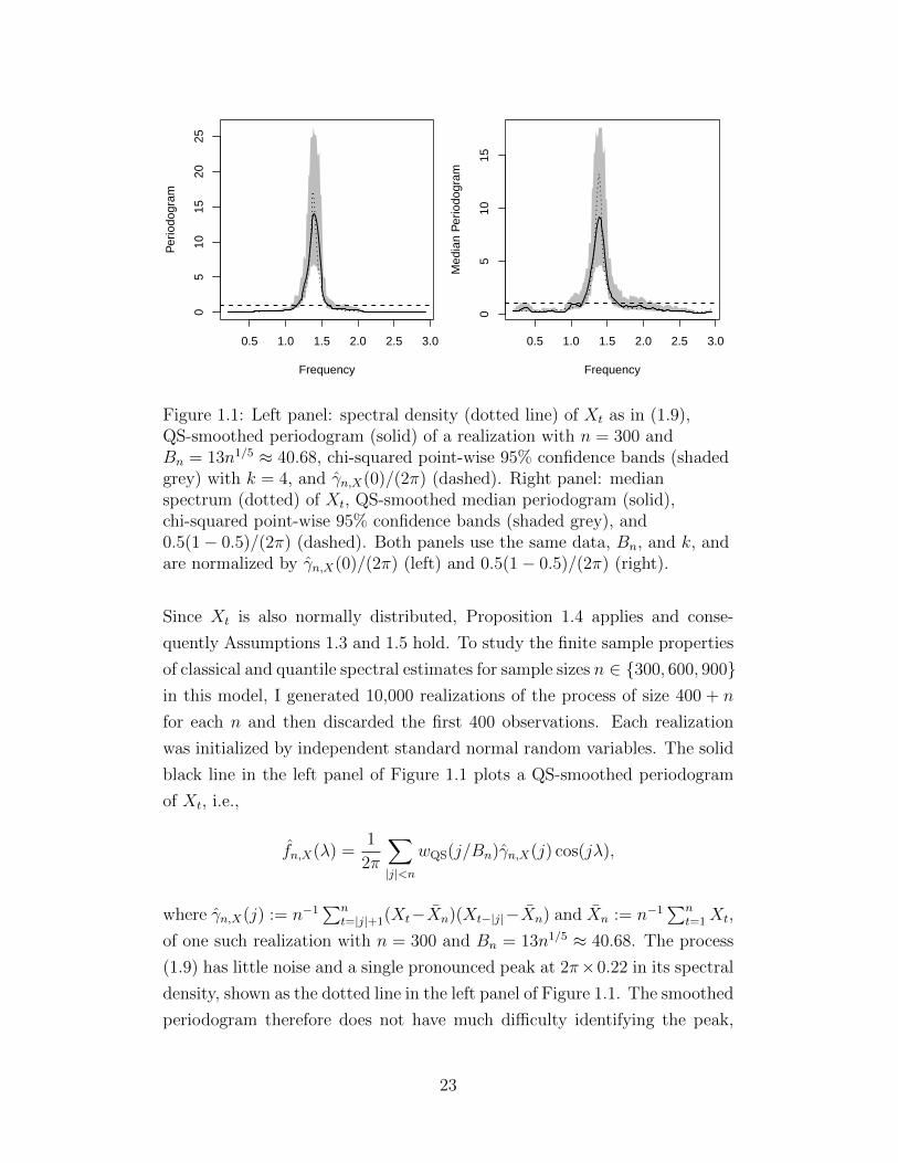
Figure 1.1: Left panel: spectral density (dotted line) of Xt as in (1.9),QS-smoothed periodogram (solid) of a realization with n = 300 andBn = 13n1/5 ≈ 40.68, chi-squared point-wise 95% confidence bands (shadedgrey) with k = 4, and γn,X(0)/(2π) (dashed). Right panel: medianspectrum (dotted) of Xt, QS-smoothed median periodogram (solid),chi-squared point-wise 95% confidence bands (shaded grey), and0.5(1− 0.5)/(2π) (dashed). Both panels use the same data, Bn, and k, andare normalized by γn,X(0)/(2π) (left) and 0.5(1− 0.5)/(2π) (right).

Since Xt is also normally distributed, Proposition 1.4 applies and conse-

quently Assumptions 1.3 and 1.5 hold. To study the finite sample properties

of classical and quantile spectral estimates for sample sizes n ∈ 300, 600, 900in this model, I generated 10,000 realizations of the process of size 400 + n

for each n and then discarded the first 400 observations. Each realization

was initialized by independent standard normal random variables. The solid

black line in the left panel of Figure 1.1 plots a QS-smoothed periodogram

of Xt, i.e.,

fn,X(λ) =1

2π

∑|j|<n

wQS(j/Bn)γn,X(j) cos(jλ),

where γn,X(j) := n−1∑n

t=|j|+1(Xt−Xn)(Xt−|j|−Xn) and Xn := n−1∑n

t=1Xt,

of one such realization with n = 300 and Bn = 13n1/5 ≈ 40.68. The process

(1.9) has little noise and a single pronounced peak at 2π×0.22 in its spectral

density, shown as the dotted line in the left panel of Figure 1.1. The smoothed

periodogram therefore does not have much difficulty identifying the peak,

23

although its size is underestimated slightly due to the smoothing. The shaded

area in the left panel shows 95% asymptotic point-wise confidence bands

based on the periodogram of Xt, defined as

In,X(λ) =1

2π

∑|j|<n

γn,X(j) cos(jλ).

The point-wise confidence bands were computed by averaging over 2k + 1

periodogram coordinates at natural frequencies in the same way as in Corol-

lary 1.7, but with Qn,τ replaced by In,X . Here and in all plots below, I used

k = 4. The dashed line in the left panel plots γn,X(0)/(2π), i.e., the usual

estimate of fX if the spectrum were known to be flat. It provides a natural

point of comparison for the other quantities; in particular, it can be seen

from the left panel that the peak at 2π × 0.22 is significantly different from

a flat spectrum at the 5% level.

The right panel of Figure 1.1 analyzes the same data with quantile spectral

methods. The black line is the QS-smoothed median (i.e., 0.5-th quantile)

periodogram and the shaded area graphs 95% point-wise confidence bands

computed as described in Corollary 1.7. Here I used the same values for Bn

and k as in the left panel. The dashed line is 0.5(1 − 0.5)/(2π), i.e., the

median spectrum under the hypothesis that it is flat. The dotted line shows

the median spectrum g0.5, which can be calculated exactly from equation

(6) in Li (2008). The smoothed median periodogram clearly identifies the

peak, although the estimate of the actual size of the peak is slightly worse

than the one obtained in the left panel. However, the median spectrum is

completely contained inside the confidence bands and the peak at 2π × 0.22

differs significantly from a flat median spectrum at the 5% level.

For both panels the choice of Bn and k matters, with lower values of Bn

and higher values of k leading to smoother—but not necessarily better—

estimates: Figure 1.2 shows the mean integrated square error (MISE) of

the QS-smoothed periodogram (left panel) and the QS-smoothed median

periodogram (right) estimated from the 10,000 realizations as a function

of Bn/n1/5. Here the behavior of both methods is quite similar and the

MISEs attain their minimum at Bn/n1/5 ≈ 13 for each n ∈ 300, 600, 900,

which provides evidence that the optimal growth rate Bn = O(n1/5) for the

QS-smoothed periodogram is also a good choice for QS-smoothed quantile

24

5 10 15 20

0.0

0.2

0.4

0.6

0.8

1.0

Bn n1 5

Nor

mal

ized

MIS

E o

f f n

, X

n = 300n = 600n = 900

5 10 15 20

0.0

0.2

0.4

0.6

0.8

1.0

Bn n1 5

Nor

mal

ized

MIS

E o

f g

n, τ

n = 300n = 600n = 900

Figure 1.2: Emprical MISE of the QS-smoothed periodogram (left panel)and the QS-smoothed median periodogram (right) for three differentsample sizes as a function of Bn/n

1/5. Both panels were separatelynormalized by the respective joint maximum of the three curves.

periodograms. Further, Table 1.1 shows the empirical frequency of the event

that the 95% confidence interval at λ ∈ π × 0.22, 2π × 0.22, 3π × 0.22covered the spectrum and median spectrum, respectively, in the experiments

for k ∈ 2, 4, 6 and n as before. The confidence intervals constructed from

the periodogram and the median periodogram behaved very similar at the

three frequencies and covered the population value in nearly 95% of all cases

unless n was small and k was large. For these values both methods had low

coverage frequencies.

Robust estimators (in the sense of Huber and Ronchetti, 2009, p. 5) exhibit

stability, i.e., small deviations from the model assumptions should have small

effects on the performance of the estimator, and high breakdown resistance,

i.e., larger deviations should not cause catastrophic results. The following

two examples illustrate that classical spectral estimates are not robust to

outliers in the data, whereas quantile spectral estimators provide reliable

results in such situations.

Example 1.20 (Stability of quantile spectral estimators). Suppose that each

observation in a realization of the AR(2) process from Example 1.19 has a

probability p of being contaminated by an additional additive error com-

ponent. For this I drew iid Bernoulli(p) variables J1, . . . , Jn and iid cen-

25

Table 1.1: Finite-sample coverage frequencies of an asymptotic 95%confidence interval (CI) for the spectrum and median spectrum of theprocess in Example 1.19 at λ ∈ π × 0.22, 2π × 0.22, 3π × 0.22 as afunction of n and k.

Periodogram CI Median Periodogram CIn k π × .22 2π × .22 3π × .22 π × .22 2π × .22 3π × .22

300 2 0.940 0.931 0.937 0.937 0.982 0.9614 0.936 0.676 0.931 0.924 0.907 0.9746 0.921 0.249 0.909 0.913 0.178 0.979

600 2 0.943 0.951 0.948 0.942 0.982 0.9564 0.946 0.915 0.947 0.938 0.980 0.9626 0.944 0.774 0.941 0.926 0.930 0.965

900 2 0.950 0.951 0.948 0.948 0.974 0.9564 0.949 0.941 0.946 0.940 0.980 0.9596 0.948 0.904 0.947 0.934 0.971 0.964

tral Student t(ν) variables T1, . . . , Tn to generate the observed samples as

Sn = Xt + JtTt : t = 1, . . . , n, where the X1, . . . , Xn were taken from Ex-

ample 1.19. The spectral density of the corresponding process (Xt +JtTt)t∈Z

is

fX+JT (λ) = fX(λ) +p

2π

ν

ν − 2,

which, for any given p, can be made as large as desired by choosing ν > 2

sufficiently close to 2 without violating the assumptions of classical spectral

theory. Figure 1.3 plots fX+JT (λ) for p = 0.15 and ν = 2.001 as a dotted line

in the left panel; the median spectrum (dotted, right) needed no adjustment

because it is invariant under such contamination. The other quantities are

the same as in Figure 1.1 and the same 300 observations were used, but 46

of these were contaminated. The smoothed periodogram retains the spectral

shape and has a significant spike at 2π×0.22, but grossly underestimates the

location of the spectrum. Moreover, the confidence bands no longer contain

the spectrum at any frequency. In sharp contrast, the smoothed median pe-

riodogram is barely affected by the contamination and the confidence bands

cover the median spectrum at almost all frequencies. The hypothesis that

g0.5(2π × 0.22) = 0.5(1− 0.5)/(2π) can also be clearly rejected.

I repeated the experiment from Table 1.1 with the contaminated data.

The estimated coverage probabilities for the confidence intervals constructed

26

0.5 1.0 1.5 2.0 2.5 3.0

010

2030

4050

Frequency

Per

iodo

gram

0.5 1.0 1.5 2.0 2.5 3.0

05

1015

Frequency

Med

ian

Per

iodo

gram

Figure 1.3: Left panel: spectral density (dotted line) of the process inExample 1.20, QS-smoothed periodogram (solid) of a realization withn = 300 and Bn = 13n1/5 ≈ 40.68, chi-squared point-wise 95% confidencebands (shaded grey) with k = 4, and γn,X(0)/(2π) (dashed). Right panel:median spectrum (dotted), QS-smoothed median periodogram (solid),chi-squared point-wise 95% confidence bands (shaded grey), and0.5(1− 0.5)/(2π) (dashed). Both panels use the same data, Bn, and k, andare normalized by γn,X(0)/(2π) (left) and 0.5(1− 0.5)/(2π) (right).

from the periodogram and the median periodogram are shown in Table 1.2.

As can be seen, the presence of outliers had little effect on the performance of

the quantile spectral estimates. In sharp contrast, the coverage probability

for the classical spectrum was almost zero in most cases and 0.245 in the

best scenario (k = 2, n = 900).

The odd behavior of the classical spectral density estimates in this example

is likely due to the imprecisely estimated auto-covariances of the contami-

nated process. As Basraka, Davis, and Mikosch (2002) point out, for near-

infinite variance time series the convergence rate of sample auto-covariances

to their population equivalent is much slower than n−1/2. Since periodograms

are weighted sums of sample auto-covariances, they can be expected to in-

herit this lack of precision. In contrast, the sample auto-covariances of Vt(τ)

can be shown to converge at rate n−1/2 as long as Assumption 1.3 and a

slightly strengthened version of Assumption 1.5 hold.

Example 1.21 (Breakdown resistance of quantile spectral estimators). Now

suppose instead that each observation from Example 1.19 has a 15 per-

27

Table 1.2: Finite-sample coverage frequencies of an asymptotic 95%confidence interval (CI) for the spectrum and the median spectrum of theprocess in Examples 1.20 as a function of n and k.

Periodogram CI Median Periodogram CIn k π × .22 2π × .22 3π × .22 π × .22 2π × .22 3π × .22

300 2 0.001 0.109 0.001 0.918 0.976 0.9584 0.001 0.001 0.001 0.900 0.858 0.9656 0.001 0.001 0.001 0.886 0.089 0.972

600 2 0.001 0.208 0.001 0.928 0.976 0.9524 0.001 0.006 0.001 0.914 0.966 0.9586 0.001 0.001 0.001 0.901 0.890 0.963

900 2 0.001 0.245 0.001 0.932 0.974 0.9484 0.001 0.013 0.001 0.924 0.973 0.9576 0.001 0.002 0.001 0.912 0.953 0.957

cent chance of being contaminated by one of the iid Cauchy(0, 1) variables

C1, . . . , Cn. The observed samples then were Sn = Xt + JtCt : t = 1, . . . , nwith the X1, . . . , Xn as before. Since these outliers do not have a well defined

mean, the spectral density of the corresponding contaminated process no

longer exists. Spectral analysis by ordinary methods broke down completely

when 46 of the 300 observations used for Figure 1.1 were contaminated: The

smoothed periodogram in Figure 1.4 no longer has the expected spectral

shape and fails to give any indication of a periodicity present in the data.

A comparison of the confidence bands to the estimate of γX(0)/(2π) now

provides overwhelming evidence for the false hypothesis that the process is

white noise. In sharp contrast, the median spectrum is unaffected by the con-

tamination and the smoothed median periodogram significantly identifies the

periodicity. In addition, the confidence bands remain essentially unchanged

from Example 1.20, which is also confirmed by the coverage probability es-

timates of the confidence intervals constructed from median periodograms

provided in Table 1.3. Here the estimates were nearly identical to the ones

presented in Table 1.2 for the median spectrum. Corresponding estimates

for the classical spectrum cannot be computed because it is unbounded at

all frequencies.

For the next Monte Carlo exercise, I return to the stochastic volatility

model from Example 1.1 to illustrate that even if the classical spectrum

28

0.5 1.0 1.5 2.0 2.5 3.0

0.0

0.5

1.0

1.5

2.0

2.5

3.0

Frequency

Per

iodo

gram

0.5 1.0 1.5 2.0 2.5 3.0

05

1015

Frequency

Med

ian

Per

iodo

gram

Figure 1.4: Left panel: QS-smoothed periodogram (solid black) of arealization of the process in Example 1.21 with n = 300 andBn = 13n1/5 ≈ 40.68, chi-squared point-wise 95% confidence bands (shadedgrey) with k = 4, and γn,X(0)/(2π) (dashed). The spectral density does notexist. Right panel: median spectrum (dotted), QS-smoothed medianperiodogram (solid), chi-squared point-wise 95% confidence bands (shadedgrey), and 0.5(1− 0.5)/(2π) (dashed). Both panels use the same data, Bn,and k, and are normalized by γn,X(0)/(2π) (left) and 0.5(1− 0.5)/(2π)(right).

Table 1.3: Finite-sample coverage frequencies of an asymptotic 95%confidence interval for the median spectrum of the process in Example 1.21as a function of n and k.

Median Periodogramn k π × .22 2π × .22 3π × .22

300 2 0.904 0.971 0.9574 0.889 0.827 0.9606 0.861 0.059 0.966

600 2 0.915 0.973 0.9484 0.901 0.961 0.9526 0.884 0.872 0.955

900 2 0.918 0.970 0.9514 0.905 0.966 0.9526 0.883 0.940 0.951

29

shows no sign of periodicity, almost all quantiles of the distribution can be

crossed in a periodic manner.

Example 1.22 (Stochastic volatility, continued). Take (εt)t∈Z to be iid copies

of an N(0, θ2) variable and let ut = log v(εt−1, εt−2, . . . ) be the stationary so-

lution of the process ut = β1ut−1 + β2ut−2 + εt−1 with β1, β2 as in (1.9).

Then eut is log-normally distributed and Xt = εtv(εt−1, εt−2, . . . ) = εteut has

median zero. To show that Xt is GMC, apply the Mean Value Theorem

and the Cauchy-Schwarz inequality to obtain the bound ‖Xn − X ′n‖α ≤‖εn‖α‖eun‖2α‖un − u′n‖2α, where u′n is un with (ε0, ε−1, . . . ) replaced by

(ε∗0, ε∗−1, . . . ) and un lies on the line segment joining un and u′n. By mono-

tonicity of the exponential function and the Minkowski inequality, we have

‖eun‖min1,2α ≤∥∥max

eun , e−un , eu

′n , e−u

′n∥∥

min1,2α ≤ 4‖eun‖min1,2α <∞

because the four terms inside the maximum have the same log-normal dis-

tribution. If needed, the Loeve cr inequality provides a similar bound for the

case 0 < 2α < 1. The GMC property then follows since ut is GMC by The-

orem 5.2 of Shao and Wu (2007). The distribution function of Xt is given

by FX(x) = EΦ(x/(eutθ)), which can be seen to have a bounded density

with the help of the Lebesgue Dominated Convergence Theorem. Therefore,

Assumptions 1.3 and 1.5 again hold.

The top two panels of Figure 1.5 graph the same spectral estimates as

in Figures 1.1 for n = 600 observations of the stochastic volatility model

with θ = 1. The spectrum (not shown to prevent clutter) and the median

spectrum (identical to the dashed line in the top right panel) of the model

are flat, which is also correctly identified at almost all frequencies by both

point-wise confidence bands. The bottom two panels show the smoothed

quantile periodograms (black lines) and point-wise confidence bands (shaded

grey) at τ = 0.25 (left) and τ = 0.75 (right) computed from the same data.

In both panels, the estimated quantile spectra show a considerable spike that

is significantly different from a flat τ -th quantile spectrum at frequency 2π×0.22, thereby providing evidence of a dependence structure that is not present

in the mean and auto-covariance of the process. Since the quantile spectra of

the process do not possess a closed-form expression for τ 6= 0.5, I instead also

plot smoothed quantile periodograms of n = 106 observations at τ = 0.25

(left) and τ = 0.75 (right) as dotted lines in the bottom panels to illustrate

30

0.5 1.0 1.5 2.0 2.5 3.0

01

23

4

Frequency

Per

iodo

gram

0.5 1.0 1.5 2.0 2.5 3.0

01

23

4

Frequency

Med

ian

Per

iodo

gram

0.5 1.0 1.5 2.0 2.5 3.0

02

46

810

12

Frequency

0.25

−th

Qua

ntile

Per

iodo

gram

0.5 1.0 1.5 2.0 2.5 3.0

02

46

810

Frequency

0.75

−th

Qua

ntile

Per

iodo

gram

Figure 1.5: Top left panel: QS-smoothed periodogram (solid) of arealization of the process in Example 1.22 with n = 600 andBn = 13n1/5 ≈ 46.73, chi-squared point-wise 95% confidence bands (shadedgrey) with k = 4, and γn,X(0)/(2π) (dashed). Other panels: QS-smoothedτ -th quantile periodogram (solid), chi-squared point-wise 95% confidencebands (shaded grey), and τ(1− τ)/(2π) (dashed) for τ = 0.5 (top right),0.25 (bottom left), and 0.75 (bottom right). All panels use the same data,Bn, and k. The top left panel is normalized by γn,X(0)/(2π). The otherpanels are normalized by τ(1− τ)/(2π). The bottom two panels also showQS-smoothed τ -th quantile periodograms (dotted) with n = 106 forτ = 0.25 (left) and 0.75 (right). Frequencies near zero are not shown toenhance readability.

31

how much of the spectral shape is already recovered in a sample with 600

observations. Indeed, although the estimates from the smaller sample are

more volatile, the size and shape of the peaks at 2π×0.22 are nearly identical

for the two sample sizes.

0.2 0.4 0.6 0.8

0.0

0.2

0.4

0.6

0.8

1.0

τ

Dis

cove

ry R

ate

n = 300n = 600n = 900

Figure 1.6: Empirical size and power of a test for a cycle with frequency2π × 0.22 in the stochastic volatility model of Example 1.22 as a function ofτ . Nominal size at τ = 0.5 is 0.05 (lower grey line).

To evaluate how reliably the quantile spectral estimates discover the cycle

at frequency 2π × 0.22, I recorded the relative number of the test decisions

in favor of the hypothesis H0 : gτ (2π × 0.22) = τ(1 − τ)/(2π) in 10,000 re-

alizations of the stochastic volatility model using a 95% confidence interval

with k = 4. The results are shown in Figure 1.6 for different sample sizes

as a function of τ ∈ (0, 1). At τ = 0.5, the null hypothesis is true and the

tests almost attained the 5% level (lower grey line) for the three sample sizes.

At the other quantiles, the null hypothesis is false, which was also correctly

recognized at all sample sizes as long as a quantile not too close to τ = 0.5

was chosen.

The additional information obtained from quantile spectral analysis can

also be seen in Figure 1.7, where I graph the QS-smoothed quantile pe-

riodogram as a function of both λ and τ . Here I chose n = 900 and

Bn = 8n1/5 ≈ 31.18 for a smoother appearance of the plot. The two humps

in the figure make it clear that most of the dependence structure is in fact

present near the lower and upper quartiles of the process, whereas working

with the mean or median provides no insight in this case.

32

0.20.4

0.60.8

0.5

1.0

1.5

2.0

2.5

0.2

0.4

0.6

0.8

1.0

τ

λ

Figure 1.7: QS-smoothed quantile periodogram across all quantiles of arealization of the process in Example 1.22 with n = 900 andBn = 8n1/5 ≈ 31.18, normalized by the joint maximum of all quantileperiodograms. Frequencies near zero are not shown to enhance readability.

The following examples illustrate the size and power of the two Cramer-von

Mises tests introduced in section 1.4.

Example 1.23 (QAR(2) and Procedure 1.15). Table 1.4 shows the empirical

rejection frequency of the null hypothesis of a flat τ -th quantile spectrum as a

function of n ∈ 100, 200, 300 and τ ∈ 0.1, 0.5, 0.9 in a variety of settings.

For each entry, I recorded the test decision of Procedure 1.15 in 10,000 real-

izations by comparing the test statistics to 5% critical values obtained from

106 simulations each. The first column of the “Size” portion provides the re-

jection frequencies when the data were iid χ23 variables. In this case, the null

hypothesis is true at all quantiles. The test behaved mildly conservatively

for τ = 0.1 in smaller samples, but was close to the level of the test at other

quantiles and samples sizes. In samples larger than 300 (not reported), the

test was essentially exact at all quantiles. I also experimented with other dis-

tributions, including normal, Student t(2), and standard Cauchy variables,

but found that they had little impact on the results.

The first column of the “Power” portion shows the relative number of

rejections when the data-generating process was the AR(2) from Example

1.19. Here the null hypothesis is false at all quantiles, which was also reliably

33

Table 1.4: Rejection frequencies of the null hypothesis for the Monte CarloCramer-von Mises test (Procedure 1.15) at the 5% level.

Size Powern τ χ2

3 Ex. 1.22 QAR Ex. 1.19 Ex. 1.22 QAR100 0.1 0.022 – 0.024 0.093 0.007 –

0.5 0.053 0.068 – 0.999 – 0.9990.9 0.037 – – 0.169 0.332 0.993

200 0.1 0.019 – 0.021 0.405 0.043 –0.5 0.052 0.076 – 1.000 – 1.0000.9 0.046 – – 0.504 0.468 1.000

300 0.1 0.048 – 0.029 0.795 0.188 –0.5 0.052 0.080 – 1.000 – 1.0000.9 0.050 – – 0.875 0.724 1.000

identified at the median at all samples. However, at the outer quantiles the

spectral peak is smaller and therefore larger samples were needed to detect

its presence. The results for the contaminated processes from Examples 1.20

and 1.21 are not shown because they were virtually identical.

The second “Size” and “Power” columns give the rejection frequencies

for the stochastic volatility model from Example 1.22. The null hypothesis is

true at τ = 0.5, but the process is not covered by the assumptions underlying

the Monte Carlo test because the stochastic volatility model is not iid, which

resulted in a mild over-rejection at all sample sizes. At the other quantiles,

the process satisfies H1 and the test has power against this alternative by

Corollary 1.16(ii). The power of the test increased sharply with the sample

size for τ = 0.9, whereas for τ = 0.1 the increase was considerably slower.

Some intuition for this result can be gathered from Figure 1.5, where the

estimated quantile spectrum in the lower quantiles can be seen to have a long

stretch on which it is close to the hypothetical quantile spectrum implied by

the null hypothesis. In contrast, this stretch is somewhat shorter in the upper

quantiles. Moreover, as shown in Figure 1.6, the setup for the test is quite

demanding because the spectral peak near the extremes of the distribution is

small. Larger samples (not reported) yielded better results, with the power

being nearly one at all quantiles for n = 600.

The third columns of the “Size” and “Power” portions show the relative

number of rejections of the hypothesis of a flat τ -th quantile spectrum for

34

realizations of the QAR(2) process (see Example 1.2)

Xt = 4 + Φ−1(εt)︸ ︷︷ ︸β0(εt)

+ 0.8× 1εt > 0.2︸ ︷︷ ︸β1(εt)

Xt−1 + 0.6× 1εt > 0.6︸ ︷︷ ︸β2(εt)

Xt−2 (1.10)

where, as before, (ε)t∈Z is a sequence of iid copies of a Uniform(0, 1) variable.

By Theorem 5.1 of Shao and Wu (2007), this recursion admits a station-

ary solution of the form (1.5) and satisfies the GMC property. Further,

the marginal distribution function of Xt can be seen to possess a bounded

Lebesgue density from the properties of truncated normal variables and dom-

inated convergence. If (Xt)t∈Z is positive, the right-hand side of (1.10) is

guaranteed to be increasing in εt conditional on Xt−1, Xt−2 and the model in

the preceding display is indeed a proper QAR model. Since the process has a

very small probability of generating a negative observation, I therefore con-

sidered only positive realizations of (1.10) in order to enforce well-behaved

sample paths.

The QAR process satisfies the null hypothesis of a flat quantile spectrum

for τ ∈ (0, 0.2] and the alternative at the other quantiles. In particular,

it behaves like a stationary QAR(1) on τ ∈ (0.2, 0.6] that exhibits enough

mean reversion to regulate the explosive behavior of the process on τ ∈(0.6, 1). This dependence structure induces an asymmetric spectral shape

across quantiles, with spectral peaks of different sizes at frequency zero in

the middle to upper quantiles. The QS-smoothed quantile periodogram of a

realization with n = 900 plotted in Figure 1.8 illustrates this shape. As can

be seen from Table 1.4, the Monte Carlo Cramer-von Mises test very reliably

detected the presence of the alternative hypothesis at τ = 0.5 and 0.9 even

for n = 100. At τ = 0.1 the null hypothesis is true and, although Procedure

1.15 does not apply because the observations are not iid, the test was only

mildly conservative.

Example 1.24 (QAR(2) and Procedure 1.17). I repeated the experiments

outlined in the previous example with the wild bootstrap test described in

Procedure 1.17. I experimented with the block size bn, but found that the

results were not overly sensitive to this choice as long as the blocks were not

too large. I therefore settled for block sizes near√n/2 and used bn = 5, 8,

and 10 for n = 100, 200, and 300, respectively, although other choices are

clearly possible; see Shao (2011a) for a thorough discussion.

35

0.20.4

0.60.8

−2

−1

0

1

2

0.2

0.4

0.6

0.8

1.0

τ

λ

Figure 1.8: QS-smoothed quantile periodogram across all quantiles of arealization of the QAR(2) process in Example 1.23 with n = 900 andBn = 8n1/5 ≈ 31.18, normalized by the joint maximum of all quantileperiodograms.

The results are shown in Table 1.5. The important difference to the pre-

ceding example is that the QAR(2) model (1.10) is now fully covered by the

assumptions of the test; see Theorem 1.18. This is also reflected in the test

for a flat quantile spectrum of the QAR process at τ = 0.1, which was nearly

exact for n = 300. The other results in the “Size” portion of the table were

similar to the ones given in Table 1.4 for the Monte Carlo test. The power

of the bootstrap test was also comparable to the other test, but neither of

the tests dominated the other: For the AR model both test behaved sim-

ilarly, for the stochastic volatility model the bootstrap test showed a more

balanced performance, and for the QAR model the Monte Carlo test was

more powerful at the outer quantiles.

Example 1.25 (Building permits data). Finally, to illustrate what kind of

insights quantile spectral analysis of actual economic data can provide, I con-

sider the series “New Privately Owned Housing Units Authorized by Building

Permits in Permit-Issuing Places” from the US Census.1 The data consist

of 634 (seasonally unadjusted) monthly observations from January 1959 to

October 2011 of the total number of permits from permit-issuing places in

1I downloaded the data from http://www.census.gov/const/permits cust.xls onNovember 30, 2011.

36

Table 1.5: Rejection frequencies of the null hypothesis for the bootstrapCramer-von Mises test (Procedure 1.17) at the 5% level. The block sizesare bn = 5, 8, and 10 for n = 100, 200, and 300, respectively. I used thewarp-speed method of Giacomini et al. (2007) to estimate size and power ofthe bootstrap test; this method considerably sped up the simulationsbecause only one bootstrap replication per Monte Carlo replication wasneeded.

Size Powern τ χ2

3 Ex. 1.22 QAR Ex. 1.19 Ex. 1.22 QAR100 0.1 0.027 – 0.026 0.113 0.056 –

0.5 0.055 0.094 – 1.000 – 0.9990.9 0.029 – – 0.170 0.110 0.374

200 0.1 0.031 – 0.030 0.430 0.339 –0.5 0.058 0.083 – 1.000 – 1.0000.9 0.049 – – 0.486 0.422 0.635

300 0.1 0.050 – 0.051 0.754 0.550 –0.5 0.056 0.090 – 1.000 – 1.0000.9 0.052 – – 0.780 0.567 0.820

the United States that report to the Census. Such a permit is typically issued

by a town or a county and enables an individual to begin construction on a

new housing unit.

Figure 1.9 graphs this time series in the frequency domain: The smoothed

periodogram (solid line, top left) and smoothed median periodogram (solid,

top right) behave similarly and have their largest peaks at frequencies 0.045

and 0.039, respectively, which translates into an estimated business cycle

length of 11.58 years when measured by the smoothed periodogram and

13.39 years when measured by the smoothed median periodogram. Both

lines also have peaks of similar size at the yearly (2π/12 ≈ 0.52) and half-

yearly (2π/6 ≈ 1.05) frequencies, which provides evidence of considerable

seasonality in the data. However, as illustrated by the smoothed 0.10-th

quantile periodogram (solid, bottom left) and 0.90-th quantile periodogram

(solid, bottom right), these seasonal cycles do not appear uniformly across

the distribution of the data. At the 0.90-th quantile, the yearly and—to

some extent—the half-yearly cycles are still present, but at the 0.10-th quan-

tile, this seasonality vanishes completely; the smoothed 0.10-th quantile pe-

riodogram also has some smaller peaks between 0.2 and 0.5, but comparison

37

0.0 0.5 1.0 1.5 2.0 2.5 3.0

05

1015

2025

Frequency

Per

iodo

gram

0.0 0.5 1.0 1.5 2.0 2.5 3.0

05

1015

FrequencyM

edia

n P

erio

dogr

am

0.0 0.5 1.0 1.5 2.0 2.5 3.0

05

1015

Frequency

0.10

−th

Qua

ntile

Per

iodo

gram

0.0 0.5 1.0 1.5 2.0 2.5 3.0

05

1015

Frequency

0.90

−th

Qua

ntile

Per

iodo

gram

Figure 1.9: Top left panel: QS-smoothed periodogram (solid) of buildingpermit data with Bn = 28n1/5 ≈ 101.76 to prevent smaller peaks from beingsmoothed out, chi-squared point-wise 95% confidence bands (shaded grey,not shown completely to prevent clutter) with k = 4, and γn,X(0)/(2π)(dashed). Other panels: QS-smoothed τ -th quantile periodogram (solid),chi-squared point-wise 95% confidence bands (shaded grey), andτ(1− τ)/(2π) (dashed) for τ = 0.5 (top right), 0.10 (bottom left), and 0.90(bottom right). All panels use the same data, Bn, and k. The top left panelis normalized by γn,X(0)/(2π). The other panels are normalized byτ(1− τ)/(2π).

38

to the confidence intervals (shaded grey) shows that these peaks are not sig-

nificantly different from a straight line. All graphs have in common, however,

that the business cycle explains most of the cyclical variation, which indicates

that seasonal patterns disappear during economic troughs.

1.6 Conclusion

In this chapter I introduced quantile spectral densities that summarize the

cyclical behavior of time series across their whole distribution by analyzing

periodicities in quantile crossings. I discussed robust spectral estimation and

inference in situations where the dependence structure of a time series is not

accurately captured by the auto-covariance function, in particular when the

time series under consideration is uncorrelated or heavy-tailed. I established

the statistical properties of quantile spectral estimators in a large class of non-

linear time series models and discussed inference both at fixed and across all

frequencies. Monte Carlo experiments and an empirical example showed that

quantile spectral estimates are similar to regular spectral density estimates

in both shape and interpretation when standard conditions are satisfied, but

can still reliably identify dependence structures when these conditions fail to

hold.

1.7 Proofs

Throughout this section, P∗ and E∗ respectively denote outer probability

and outer expectation (see, e.g., van der Vaart, 1998, p. 258). Probability

and expectation conditional on the observed sample Sn is abbreviated by

P(·) := P(· | Sn) and E(·) := E(· | Sn).

Proof of Proposition 1.4. By assumption, we can find a δ′ > 0 such that FX

is Lipschitz on (ξ0(τ) − δ′, ξ0(τ) + δ′). Choose a large enough N ∈ N such

that δ := δ′ − %N/(1+α) > 0 and pick any ξ ∈ Xτ (δ); then, for all n ≥ N ,

apply the pointwise bound

|1Xn < ξ − 1X ′n < ξ| ≤ 1|Xn − ξ| < |Xn −X ′n|,

39

the Markov inequality, and the GMC property to see that

‖1Xn < ξ − 1X ′n < ξ‖2

≤ P(|Xn − ξ| < |Xn −X ′n|)

≤ P(|Xn − ξ| < %nα/(1+α)) + E |Xn −X ′n|α%−nα2/(1+α)

≤M%nα/(1+α)

for a large enough absolute constant M . This constant can be enlarged

slightly to ensure that the inequality also holds for the remaining n < N .

With σ := %α/(2+2α), take square-roots on both sides and suprema over Xτ (δ)to establish the desired result.

Proof of Theorem 1.6. Let Zt,n = (Xt, tλn) and define the maps hξ(Zt,n) =

1Xt < ξ × cos(tλn) and h∗ξ(Zt,n) = 1Xt < ξ × sin(tλn). The empirical

process evaluated at some function h is denoted by

νn h := n−1/2

n∑t=1

(h(Zt,n)− Eh(Zt,n)

).

The finite Fourier transform at nonzero natural frequencies is invariant to

centering. Hence, from (1.3), we can decompose Qn,τ (λn) into

1

2π

∣∣∣νn(hξn(τ) − hξ0(τ)

)+ i νn

(h∗ξn(τ)− h∗ξ0(τ)

)− n−1/2

n∑t=1

Vt(τ)e−itλn∣∣∣2(1.11)

For the proof of the theorem, I proceed in three steps: I show that (i) the first

term and (ii) the second term inside the modulus in the display are small in

probability and that (iii) the remainder of (1.11) has the desired asymptotic

distribution jointly for frequencies λn + 2πj/n with |j| ≤ k.

Step (i): Define a norm ρ(hξ) = supt,n∈N ‖hξ(Zt,n)‖. Take a grid of points

ξ0(τ)− δ =: ξ0 < ξ1 < · · · < ξN := ξ0(τ) + δ and let bk(Zt,n) :=(hξk(Zt,n,)−

hξk−1(Zt,n)

)/ cos(tλn). Given a ξ ∈ Xτ (δ), we can then find an index k such

that |hξ − hξk−1| ≤ bk. In addition, we have

ρ(bk) = ‖1X0 < ξk − 1X0 < ξk−1‖ ≤√FX(ξk)− FX(ξk−1),

which is bounded above by a constant multiple of√ξk − ξk−1 due to Lipschitz

40

continuity. Hence, if we choose the grid such that ρ(bk) ≤ ε for all k =

1, . . . , N , the parametric class H := hξ : ξ ∈ Xτ (δ) has bracketing numbers

(see Andrews and Pollard, 1994; van der Vaart, 1998, pp. 270-271) with

respect to ρ of order N(ε,H) = O(ε−2) as ε→ 0.

By the same calculations as in the preceding display, there is some M > 0

such that all ξ, ξ′ ∈ Xτ (δ) satisfy ρ(hξ − hξ′) ≤ M |ξ − ξ′|1/2 and therefore

ρ(hξn(τ) − hξ0(τ)) →p 0 in view of Lemma 1.26 below. For ε, η > 0, the limit

superior of P(| νn(hξn(τ) − hξ0(τ))| ≥ ε

)is then at most

lim supn→∞

P(∣∣νn(hξn(τ) − hξ0(τ)

)∣∣ ≥ ε, ρ(hξn(τ) − hξ0(τ)

)≤ η)

≤ lim supn→∞

P∗(

supξ∈Xτ (δ):ρ(hξ−hξ0(τ))≤η

∣∣νn(hξ − hξ0(τ)

)∣∣ ≥ ε

)(1.12)

The Markov inequality and Lemma 1.28 below imply that the term on the

right can be made as small as desired by choosing η small enough. This is

also true for the frequencies λn + 2πj/n with |j| ≤ k.

Step (ii): Replace cosines with sines in the proofs of Lemmas 1.27 and 1.28

(with the same bounding functions bk as above) to reach the same conclusion

for νn(h∗ξ0(τ) − h∗ξn(τ)).

Step (iii): In view of (i), (ii), and continuity of the modulus, I only have

to show that the remainder of (1.11) converges jointly at each λn + 2πj/n,

|j| ≤ k, in distribution to independent exponential variables with mean gτ (λ).

For this I apply Corollary 2.1 of Shao and Wu (2007). Because Vt(τ) is a

bounded mean-zero variable, the only condition that has to be checked is

∞∑t=0

‖E(Vt(τ) | F0)− E(Vt(τ) | F−1)‖ <∞.

By the conditional Jensen inequality, the law of iterated expectations, and

Assumption 1.9, this summability condition is satisfied because

∥∥E(Vt(τ) | F0

)− E

(Vt(τ) | F−1

)∥∥=∥∥E(1Xt < ξ0(τ) − 1X∗t < ξ0(τ) | F0

)∥∥≤ ‖1Xt < ξ0(τ) − 1X∗t < ξ0(τ)‖.

Assumption 1.3 implies Assumption 1.9, and so the joint convergence asserted

41

in Theorem 1.6 follows.

Lemma 1.26. Suppose Assumptions 1.5 and 1.9 hold; then ξn(τ) − ξ0(τ) =

Op(n−1/2).

Proof of Lemma 1.26. Arguing as in the proof of Theorem 1 of Wu (2005),

use the conditional Jensen inequality and the law of iterated expectations to

deduce that

‖E(1Xt < ξ | F0)− E(1X∗t < ξ | F−1, ε∗0)‖

= ‖E(1Xt < ξ − 1X∗t < ξ | F0, ε∗0)‖

≤ ‖1Xt < ξ − 1X∗t < ξ‖.

Taking suprema over Xτ (δ) shows that Assumption 1.9 implies condition (7)

of Wu (2007) and his Theorem 1 then yields the desired result.

For Lemmas 1.27 and 1.28, I mimic the proofs of Andrews and Pollard’s

(1994) Theorem 2.2 and Lemma 3.1; their arguments do not apply directly

since Andrews and Pollard work with strongly mixing arrays.

Lemma 1.27. Let φ(hξ−hξ′) := ρ(hξ−hξ′)2/(2+γ) for some γ > 0 and suppose

that Assumption 1.3 holds. Then, for all n ∈ N, all ξ, ξ′ ∈ Xτ (δ), and every

even integer Q ≥ 2,

E | νn(hξ − hξ′)|Q ≤ n−Q/2C((φ(hξ − hξ′)2n) + · · ·+ (φ(hξ − hξ′)2n)Q/2

),

where C depends only on Q, γ, and σ. The inequality remains valid when

hξ − hξ′ is replaced by bk for any given k ≥ 1.

Proof of Lemma 1.27. It suffices to show the inequality given in the lemma

after dividing both sides by 4Q to ensure that the absolute value of

Ht :=(hξ(Zt,n)− hξ′(Zt,n)− (Ehξ(Zt,n)− Ehξ′(Zt,n))

)/4

is bounded by 1. The 4−Q on the right hand can be absorbed into C. Define

H ′t in the same way as Ht but replace Xt with X ′t. Here I suppress the

dependence of Ht and H ′t on n, ξ, and ξ′ because they are irrelevant in the

following. Also note that EHt = EH ′t = 0 for all t, n ∈ N and all ξ, ξ′ ∈ Xτ (δ)because Xt and X ′t are identically distributed.

42

For fixed k ≥ 2, d ≥ 1, and 1 ≤ m < k, consider integers t1 ≤ · · · ≤ tm ≤tm+1 ≤ · · · ≤ tk so that tm+1−tm = d and define ak(λn) = |2−k

∏ki=1 cos(tiλn)|.

Since Ut := Ht/ cos(tλn) and U ′t := H ′t/ cos(tλn) are stationary, repeatedly

add and subtract to see that

∣∣EHt1Ht2 · · ·Htk − EHt1Ht2 · · ·Htm EHtm+1 · · ·Htk

∣∣= ak(λn)

∣∣EUt1−tmUt2−tm · · ·Utk−tm − EUt1−tmUt2−tm · · ·U0 EUd · · ·Utk−tm∣∣

≤ ak(λn)∣∣EUt1−tm · · ·U0(Ud − U ′d)Utm+2−tm · · ·Utk−tm

∣∣+

k−m−1∑i=2

ak(λn)∣∣EUt1−tm · · ·U0U

′d · · · (Utm+i−tm − U ′tm+i−tm) · · ·Utk−tm

∣∣+ ak(λn)

∣∣EUt1−tm · · ·U0U′d · · ·U ′tk−tm − EUt1−tm · · ·U0 EUd · · ·Utk−tm

∣∣(1.13)

In particular, the last term on the right-hand side is zero because Ut1−tm · · ·U0

and U ′d · · · U ′tk−tm are independent and U ′d · · ·U ′tk−tm and Ud · · ·Utk−tm are

identically distributed.

By Assumption 1.3, ‖Ud − U ′d‖s ≤ ‖1Xd < ξ − 1X ′d < ξ‖s + ‖1Xd <

ξ′−1X ′d < ξ′‖s ≤ 2 supξ∈Xτ (δ) ‖1Xd < ξ−1X ′d < ξ‖s ≤ C ′σd for some

C ′ > 0 and s ≥ 1. Here the choice of s does not matter because Assumption

1.3 still applies when ‖ · ‖ is replaced by ‖ · ‖s for any s > 0; see Lemma 2 of

Wu and Min (2005). Holder’s inequality then bounds the first term on the

right-hand side of the preceding display by

‖Ht1 · · ·Htm‖p‖Htm+2 · · ·Htk‖qC ′σd, (1.14)

where the reciprocals of p, q, and s sum to 1. Proceeding as in Andrews and

Pollard (1994), another application of the Holder inequality yields

‖Ht1 · · ·Htm‖p ≤( m∏i=1

E |Hti |mp)1/(mp)

≤ φ(hξ − hξ′)(2+γ)/p

whenevermp ≥ 2 and similarly ‖Htm+2 · · ·Htk‖q ≤ φ(hξ−hξ′)(2+γ)/q whenever

(k − m − 1)q ≥ 2. Suppose for now that k ≥ 3. If k > m + 1, take

s = (γ + Q)/γ and mp = (k − m − 1)q = (k − 1)/(1 − 1/s). Decrease

the resulting exponent of φ(hξ − hξ′) from Q(2 + γ)/(Q + γ) to 2 to see

that (1.14) is bounded by C ′σdφ(hξ − hξ′)2. If k ≥ 2 and k = m + 1,

43

the factor ‖Htm+2 · · ·Htk‖q is not present in (1.14), but we can still choose

s = (γ +Q)/γ and mp = (k− 1)/(1− 1/s) to obtain the same bound. Since

the same argument also applies to each of the other summands in (1.13), we

can find a constant M > 0 such that

∣∣EHt1Ht2 · · ·Htk

∣∣ ≤ ∣∣EHt1Ht2 · · ·Htm EHtm+1 · · ·Htk

∣∣+Mσdφ(hξ − hξ′)2.

Here M in fact depends on k, but this does not disturb any of the subsequent

steps.

Now replace (A.2) in Andrews and Pollard (1994) by the inequality in the

preceding display. In particular, replace their 8α(d)1/s with Mσd and their

τ 2 with φ(hξ − hξ′)2. The rest of their arguments now go through without

changes.

The inequality for bk follows by letting λn ≡ 0; this is not a contradiction to

the assumptions of Theorem 1.6 because this proof is valid for any sequence

(λn)n∈N.

Lemma 1.28. Suppose the assumptions of Theorem 1.6 hold. For every ε > 0

and every even integer Q ≥ 4, there is an η > 0 such that

lim supn→∞

E∗(

supξ,ξ′∈Xτ (δ):ρ(hξ−hξ′ )≤η

| νn(hξ − hξ′)|)Q≤ ε.

Proof of Lemma 1.28. I follow Andrews and Pollard’s (1994) proof of their

Theorem 2.1. It requires three steps: (i) Their “Proof of inequality (3.2),”

(ii) their “Proof of inequality (3.3),” and (iii) their “Comparison of pairs”

argument. Replace their i with k and their τ(hi) with φ(bk); then apply

Lemma 1.27 above instead of Andrews and Pollard’s (1994) Lemma 3.1 in

the derivation of their inequality (3.5) to deduce∥∥∥ max1≤k≤N

| νn bk|∥∥∥Q≤ C ′N1/Q max

n−1/2, max

1≤k≤Nφ(bk)

and use this inequality in (i) instead of their inequality (3.5). In (i) Andrews

and Pollard also require the finiteness of the bracketing integral∫ 1

0

x−γ/(2+γ)N(x,H)1/Q dx,

44

which follows immediately by choosing γ = Q − 4. Another application

of Lemma 1.27 establishes the required analogue of Andrews and Pollard’s

inequality (3.5) used in (ii). The same inequality can also be applied in (iii).

The other arguments remain valid without changes.

Proof of Theorem 1.11. Denote by rn,τ (j) = n−1∑n|j|+1 Vt(τ)Vt−|j|(τ) and

gn,τ (λ) :=1

2π

∑|j|<n

w(j/Bn)rn,τ (j)e−ijλ

the infeasible sample auto-covariance and smoothed quantile spectrum, re-

spectively, based on the unknown quantile ξ0(τ). The triangle inequality and

|Vt(·, ·)| < 1 yield

2π supλ∈(−π,π]

|gn,τ (λ)− gn,τ (λ)|

≤ 1

n

∑|j|<n

|w(j/Bn)|n∑

t=|j|+1

|Vt(τ)Vt−|j|(τ)− Vt(τ)Vt−|j|(τ)|

≤ 1

n

∑|j|<n

|w(j/Bn)|n∑

t=|j|+1

(|Vt(τ)− Vt(τ)|+ |Vt−|j|(τ)− Vt−|j|(τ)|

)≤ 1

n

∑|j|<n

|w(j/Bn)|n∑

t=|j|+1

(1|Xt−ξ0(τ)|<|ξn(τ)−ξ0(τ)|

+ 1|Xt−|j|−ξ0(τ)|<|ξn(τ)−ξ0(τ)|

).

Consider the first indicator function on the right-hand side of the preceding

display and recall that√n(ξn(τ)− ξ0(τ)) is uniformly tight by Lemma 1.26.

For any given ε > 0 and η > 0, the Markov inequality implies for large

enough M > 0

lim supn→∞

P

(1

n

∑|j|<n

|w(j/Bn)|n∑

t=|j|+1

1|Xt−ξ0(τ)|<|ξn(τ)−ξ0(τ)| ≥ η

)

≤ lim supn→∞

P

(1

n

∑|j|<n

|w(j/Bn)|n∑

t=|j|+1

1|Xt−ξ0(τ)|<Mn−1/2 ≥ η

)+ sup

n∈NP(|ξn(τ)− ξ0(τ)| ≥Mn−1/2

)≤ lim sup

n→∞

1

η

∑|j|<n

|w(j/Bn)|P(|X0 − ξ0(τ)| < Mn−1/2) + ε.

45

By Lemma 1 of Jansson (2002), the limit superior of B−1n

∑|j|<n |w(j/Bn)| is

finite, and in view of the assumed Lipschitz continuity, the first term on the

right-hand side of the preceding display then vanishes because Bnn−1/2 → 0.

The same argument applies to the second indicator function above due to

stationarity. Together this yields supλ |gn,τ (λ)− gn,τ (λ)| →p 0.

To show gn,τ (λ)→p gτ (λ) uniformly in λ, I use Liu and Wu’s (2010) The-

orem 1, which applies whenever the windows w ∈ W satisfy their Condition

1. The only two conditions that need to be established are the absolute inte-

grability of w, which is immediate from∫∞−∞ |w(x)| dx ≤ 2

∫∞0w(x) dx <∞,

and

lim supn→∞

B−1n

∑j∈Z

w(j/Bn)2 <∞.

Although Liu and Wu (2010) provide a specific value for the limit in the

preceding display, its boundedness is in fact all that is needed for the proof

of their Theorem 1. To this end, take M ≥ supx∈R |w(x)| such that for j ≥ 1

w(j/Bn)2 ≤M |w(j/Bn)| ≤Mw(j/Bn) ≤MBn

∫ j/Bn

(j−1)/Bn

w(x) dx

by monotonicity, and therefore symmetry implies

B−1n

∑j∈Z

w(j/Bn)2 ≤ B−1n + 2M

∞∑j=1

∫ j/Bn

(j−1)/Bn

w(x) dx

= B−1n + 2M

∫ ∞0

w(x) dx,

which is finite by assumption. This is also true for its limit superior as

n→∞. The triangle inequality completes the proof.

Proof of Theorem 1.12. (i) The process Sn,τ (λ) can be decomposed into

√n

n−1∑j=1

(rn,τ (j)− rn,τ (j)

)ψj(λ) +

√n

n−1∑j=1

rn,τ (j)ψj(λ).

The second term side converges weakly in L2(Π) to Sτ (λ) by the proof of

Theorem 2.1 of Shao (2011a). The Continuous Mapping Theorem then yields

CM n,τ ‖Sτ‖2Π as long as the L2(Π)-norm of the first term of the display

is eventually small in probability.

46

To this end, define ϕj = ‖ψj‖Π and note that 〈ψj, ψk〉 = 0 for j 6= k. Use

this orthogonality to write

∥∥∥√n n−1∑j=1

(rn,τ (j)− rn,τ (j)

)ψj

∥∥∥2

Π= n

n−1∑j=1

(rn,τ (j)− rn,τ (j)

)2ϕ2j .

Let rn,τ (j, ξ) = (τ − FX(ξ))2(n − j)/n for j > 0 and ξ ∈ R. Under the null

hypothesis, we have rτ (j) = 0 = rn,τ (j, ξ0(τ)) for all j > 0 and, by Lipschitz

continuity, there exists M > 0 such that

rn,τ (j) := rn,τ (j, ξn(τ)) ≤ |FX(ξn(τ))− τ |2 ≤M |ξn(τ)− ξ0(τ)|2

for all j > 0. In view of these properties, fix some K ≤ n and apply the

Loeve cr inequality to bound the quantity in the preceding display by

2nK−1∑j=1

(rn,τ (j)− rn,τ (j)−

(rn,τ (j)− rτ (j)

))2

ϕ2j (1.15)

+ 2nK−1∑j=1

rn,τ (j)2ϕ2

j + nn−1∑j=K

(rn,τ (j)− rn,τ (j)

)2ϕ2j . (1.16)

Fix ε, ε′ > 0 and let eξ,j(Xt, Xt+j) := Vt(τ, ξ)Vt+j(τ, ξ). For given j > 0,

take ρ(eξ,j−eξ′,j) as the distance of ξ and ξ′ on Xτ (δ), where ρ is as in the proof

of Theorem 1.6. The distance also depends on τ , but this is irrelevant in the

following. Note that ρ(eξ,j−eξ′,j) ≤ 2‖1X0 < ξ−1X0 < ξ′‖ ≤M ′|ξ−ξ′|uniformly in j > 0 for some M ′ > 0 by stationarity. Hence, for any ηj > 0,

1 ≤ j < K, we have

PK−1⋃j=1

ρ(eξn(τ),j − eξ0(τ),j

)> ηj

≤ P

(|ξn(τ)− ξ0(τ)|1/2 > min

1≤j<Kηj/M

′)

= o(1).

Under the null hypothesis, we can write√n(rn,τ (j)−rτ (j)) =

√(n− j)/n×

νn−j eξ0(τ) and, by (1.8),√n(rn,τ (j) − rn,τ (j)) =

√(n− j)/n νn−j eξn(τ) as

long as ξn(τ) ∈ Xτ (δ), where I use the notation from the proof of Theorem

47

1.6. In view of the preceding display, (1.15) then satisfies

lim supn→∞

P(n

K−1∑j=1

(rn,τ (j)− rn,τ (j)−

(rn,τ (j)− rτ (j)

))2

ϕ2j ≥ ε/2

)

≤ lim supn→∞

P∗(K−1∑j=1

(sup

ξ∈Xτ (δ):ρ(eξ,j−eξ0(τ),j)≤ηj

∣∣νn−j(eξ,j − eξ0(τ),j

)∣∣)2

ϕ2j ≥ ε/2

)

≤ 2

ε

K−1∑j=1

lim supn→∞

E∗(

supξ∈Xτ (δ):ρ(eξ,j−eξ0(τ),j)≤ηj

∣∣νn−j(eξ,j − eξ0(τ),j

)∣∣)2

ϕ2j

≤ 2

ε

K−1∑j=1

(lim supn→∞

E∗(

supξ∈Xτ (δ):ρ(eξ,j−eξ0(τ),j)≤ηj

∣∣νn−j(eξ,j − eξ0(τ),j

)∣∣)Q)2/Q

ϕ2j

≤ 2ε′

ε

K−1∑j=1

ϕ2j ≤

2ε′

ε

∑j>0

ϕ2j =

( π6ε

)ε′,

where the first inequality is the Markov inequality, the second follows from

Lemma 1.29 below, the third is Jensen’s, and the equality uses ϕ2j = 1/(2πj2)

for j > 0.

Now consider (1.16). The first term can be bounded by

2nM2|ξn(τ)− ξ0(τ)|4∑j>0

ϕ2j = Op(n

−1) = op(1).

By arguments as in the proof of Theorem 1.11, for a large enough M ′ the

probability that the second term of (1.16) exceeds ε is at most

P(nn−1∑j=K

(rn,τ (j)− rn,τ (j)

)2ϕ2j ≥ ε, |ξn(τ)− ξ0(τ)| ≤M ′n−1/2

)+ ε′

≤ P

(n−1

n−1∑j=K

( n∑t=j+1

1|Xt−ξ0(τ)|<|ξn(τ)−ξ0(τ)|

+ 1|Xt−j−ξ0(τ)|<|ξn(τ)−ξ0(τ)|

)2

ϕ2j ≥ ε, |ξn(τ)− ξ0(τ)| ≤M ′n−1/2

)+ ε′

≤ P

(n−1

n−1∑j=K

( n∑t=j+1

1|Xt−ξ0(τ)|≤M ′n−1/2

)2

ϕ2j

+ n−1

n−1∑j=K

( n∑t=j+1

1|Xt−j−ξ0(τ)|≤M ′n−1/2

)2

ϕ2j ≥ ε/2

)+ ε′

48

≤ 4

εE(n−1/2

n∑t=1

1|Xt−ξ0(τ)|≤M ′n−1/2

)2∑j≥K

ϕ2j + ε′

≤ 4

ε

(P(|X0 − ξ0(τ)| ≤M ′n−1/2

)+ nP

(|X0 − ξ0(τ)| ≤M ′n−1/2

)2)∑j≥K

ϕ2j + ε′

= O(1)∑j≥K

ϕ2j + ε′,

which can be made smaller than 2ε′ by choosing K large enough. This

does not affect any of the other bounds. Since ε′ was arbitrary, we have

CM n,τ = ˜CM n,τ + op(1) and CM n,τ ‖Sτ‖2Π, which proves the first result.

(ii) Fix some K ≤ n and decompose the statistic into

CM n(τ)/n =K−1∑j=1

(rn,τ (j)− rn,τ (j)

)2ϕ2j + 2

K−1∑j=1

(rn,τ (j)− rn,τ (j)

)rn,τ (j)ϕ

2j

+K−1∑j=1

rn,τ (j)2ϕ2

j +n−1∑j=K

rn,τ (j)2ϕ2

j .

The first and second terms on the right-hand side of the displayed equation

converge to zero in probability as n → ∞ because rn,τ (j) − rn,τ (j) = op(1)

for each j under the assumptions of the theorem. The third term converges

in probability to∑K−1

j=1 rτ (j)2ϕ2

j as n → ∞ by Wu’s (2005) Theorem 2(i).

The absolute value of the last term is bounded by∑

j≥K ϕ2j , where I have

used the fact that |rn,τ | ≤ 1. Hence, let K →∞ to conclude CM n(τ)/n→p∑j>0 rτ (j)

2ϕ2j > 0. The desired result now follows from a routine argument.

Lemma 1.29. Suppose the assumptions of Theorem 1.12 hold. For every

j > 0, every Q, and every ε > 0, there is an η > 0 such that

lim supn→∞

E∗(

supξ,ξ′∈Xτ (δ):ρ(eξ,j−eξ′,j)≤η

| νn−j(eξ,j − eξ′,j)|)Q≤ ε.

Proof of Lemma 1.29. Take a grid of points ξ0(τ)−δ = ξ0 < ξ1 < · · · < ξN =

ξ0(τ) + δ and let bk,j(Xt, Xt+j) := 1Xt < ξk − 1Xt < ξk−1 + 1Xt+j <

ξk − 1Xt+j < ξk−1. Given a ξ ∈ Xτ (δ), we can then find an index k such

49

that |eξ,j − eξk−1,j| ≤ bk,j. Further,

ρ(bk,j) ≤ 2‖1X0 < ξk − 1X0 < ξk−1‖ ≤ 2√FX(ξk)− FX(ξk−1),

which is proportional to√ξk − ξk−1 due to Lipschitz continuity. If ρ(bk,j) ≤ ε

for all k = 1, . . . , N then, as above, for each j the parametric class Ej := eξ,j :

ξ ∈ Xτ (δ) has bracketing numbers with respect to ρ of order N(ε, Ej) =

O(ε−2) as ε → 0. Hence, bracketing integrals of the class H above and the

classes Ej have the same behavior. The proof of Lemma 1.28 therefore also

applies to this lemma as long as the reference to Lemma 1.27 is replaced by

Lemma 1.30 below.

Lemma 1.30. Fix some γ > 0 and suppose that Assumption 1.3 holds. For

all n ∈ N, all j < n, all ξ, ξ′ ∈ Xτ (δ), and every even integer Q ≥ 2 we have

E | νn−j(eξ,j − eξ′,j)|Q ≤ (n− j)−Q/2C((φ(eξ,j − eξ′,j)2(n− j))

+ · · ·+ (φ(eξ,j − eξ′,j)2(n− j))Q/2),

where C depends only on j, Q, γ, and σ. The inequality remains valid when

eξ,j − eξ′,j is replaced by bk,j for any given k ≥ 1.

Proof of Lemma 1.30. As in the proof of Lemma 1.27, it suffices to show the

inequality given in the Lemma after dividing both sides by 4Q to ensure that

the absolute value of

Et,t+j :=(eξ,j(Xt, Xt+j)−eξ′,j(Xt, Xt+j)−(E eξ,j(X0, Xj)−E eξ′,j(X0, Xj))

)/4

is bounded by 1. Define E ′t,t+j in the same way as Et,t+j but replace Xt with

X ′t and Xt+j with X ′t+j. For fixed k ≥ 2, d ≥ 1, and 1 ≤ m < k, consider

integers t1 ≤ · · · ≤ tm ≤ tm+1 ≤ · · · ≤ tk so that tm+1 − tm = d. Repeatedly

add and subtract to see that

∣∣EEt1,t1+j · · ·Etk,tk+j − EEt1,t1+j · · ·Etm,tm+j EEtm+1,tm+1+j · · ·Etk,tk+j

∣∣=∣∣EEt1−tm−j,t1−tm · · ·Etk−tm−j,tk−tm− EEt1−tm−j,t1−tm · · ·E−j,0 EEl−j,l · · ·Etk−tm−j,tk−tm

∣∣≤∣∣EEt1−tm−j,t1−tm · · ·E−j,0(Ed−j,d − E ′d−j,d)

× Etm+2−tm−j,tm+2−tm · · ·Etk−tm−j,tk−tm∣∣

50

+k−m−1∑i=2

∣∣EEt1−tm−j,t1−tm · · ·E−j,0E ′d−j,d × · · ·× (Etm+i−tm−j,tm+i−tm − E ′tm+i−tm−j,tm+i−tm) · · ·Etk−tm−j,tk−tm

∣∣+∣∣EEt1−tm−j,t1−tm · · ·E−j,0E ′d−j,d · · ·E ′tk−tm−j,tk−tm− EEt1−tm−j,t1−tm · · ·E−j,0 EEl−j,l · · ·Etk−tm−j,tk−tm

∣∣,where the last term on the right-hand side can again been seen to be zero.

Since j is fixed, it is possible to write ‖Ed−j,d − E ′d−j,d‖s ≤ ‖1Xd <

ξ − 1X ′d < ξ‖s + ‖1Xd−j < ξ′ − 1X ′d−j < ξ′‖s ≤ C ′σd(1 + σ−j) for

some C ′ > 0, where the cases where d ≤ j were absorbed into C ′. The same

can then be done for (1 + σ−j). Hence, proceed exactly as above to find a

constant M > 0 such that

∣∣EEt1,t1+jEt2,t2+j · · ·Etk,tk+j

∣∣≤∣∣EEt1,t1+jEt2,t2+j · · ·Etm,tm+j EEtm+1,tm+1+j · · ·Etk,tk+j

∣∣+Mσdφ(eξ,j − eξ′,j)2.

The rest of the arguments in the proof of Lemma 1.27 now go through without

changes. The proof for the bounding functions bk is almost identical and

therefore omitted.

Proof of Corollary 1.16. (i) Theorem 1 of Lifshits (1982) guarantees that

‖Sτ‖2Π has a continuous distribution function, and therefore cn,τ (1 − α) →

c∞,τ (1−α) by Lemma 21.2 of van der Vaart (1998), where c∞,τ is the quantile

function of ‖Sτ‖2Π. Hence, CM n,τ − cn,τ (1− α) ‖Sτ‖2

Π − c∞,τ (1− α) and,

in particular, ‖Sτ‖2Π− c∞(1−α) also has a continuous distribution function.

This in turn implies

∣∣P(CM n,τ > cn,τ (1− α))− α

∣∣=∣∣P(CM n,τ ≤ cn,τ (1− α)

)− P

(‖Sτ‖2

Π ≤ c∞,τ (1− α))∣∣→ 0.

(ii) Let CM∞,τ :=∑

j>0 rτ (j)2ϕ2

j and pick an ε > 0 such that CM∞,τ−ε >0. By Theorem 1.12(ii) and the properties of quantile functions,

P(CM n,τ ≤ cn,τ (1− α)

)≤ 1(cn,τ (1− α) > n(CM∞,τ − ε)

)+ P(|CM n,τ/n− CM∞,τ | ≥ ε)

51

= 1(1− α > P(CM ′

n,τ/n ≤ CM∞,τ − ε))

+ o(1).

It therefore suffices to show that CM ′n,τ/n →p 0, which follows from an

application of Birkhoff’s Ergodic Theorem to the first term on the right-

hand side of

n−1CM ′n,τ ≤

K−1∑j=1

(n−1

n∑t=1+j

(τ − Jt)(τ − Jt−j))2

ϕ2j +

∑j≥K

ϕ2j

and then letting K →∞.

Proof of Theorem 1.18. (i) Recall that rτ (j) = 0 for all j > 0 under the

null hypothesis and let r∗n,τ (j) := n−1∑n

t=j+1 Vt(τ)Vt−j(τ)ωt. We can write

CM ∗n,τ = ‖S∗n,τ‖2

Π, where S∗n,τ is

n−1/2

n−1∑j=1

( n∑t=j+1

(Vt(τ)Vt−j(τ)− Vt(τ)Vt−j(τ)

)ωt

)ψj(λ) (1.17)

− n−1/2

n−1∑j=1

rn,τ (j)ψj(λ)

( n∑t=j+1

ωt

)+√nn−1∑j=1

r∗n,τ (j)ψj(λ). (1.18)

As a preliminary step, I show that the L2(Π)-norms the first two terms have

a P-probability limit of zero with high P-probability; the L2(Π)-norm of the

third term converges P-weakly in P-probability to ‖Sτ‖2Π by Shao’s (2011a)

Theorem 3.1. I then use these results below to prove that the bootstrap test

has asymptotic size α.

The P-expectation of the square of the L2(Π)-norm of (1.17) can be written

as

E∥∥∥∥n−1/2

n−1∑j=1

( n∑t=j+1

(Vt(τ)Vt−j(τ)− Vt(τ)Vt−j(τ)

)ωt

)ψj

∥∥∥∥2

Π

= n−1

n−1∑j=1

ϕ2j

Ln∑s=1

( ∑t∈Bs∩[j+1,n]

(Vt(τ)Vt−j(τ)− Vt(τ)Vt−j(τ)

))2

.

Fix ε, ε′ > 0 and pick a large enough M > 0 such that supn∈N P(|X0−ξ0(τ)| >Mn−1/2) < ε′. As in the proof of Theorem 1.12(i), the probability that the

52

term on the right is larger than ε is at most ε′ plus

2

ε

n−1∑j=1

ϕ2jn−1

Ln∑s=1

E( ∑t∈Bs∩[j+1,n]

1|Xt−ξ0(τ)|≤Mn−1/2

)2

≤ 2

ε

n−1∑j=1

ϕ2jb−1n

(bn P

(|X0 − ξ0(τ)| ≤Mn−1/2

)+ b2

n P(|X0 − ξ0(τ)| ≤Mn−1/2

)2)

≤ 2

ε

(O(n−1/2) +O(bn/n)

)∑j>0

ϕ2j ,

which can be made arbitrarily small by first letting n→∞ and thenM →∞.

Now consider the P-expectation of the square of the L2(Π)-norm of (1.18),

which can be written as

E∥∥∥∥n−1/2

n−1∑j=1

rn,τ (j)

( n∑t=j+1

ωt

)ψj

∥∥∥∥2

Π

= n−1

n−1∑j=1

rn,τ (j)2ϕ2

j

Ln∑s=1

E( ∑t∈Bs∩[j+1,n]

ωt

)2

≤ bn

n−1∑j=1

rn,τ (j)2ϕ2

j

≤ 2bn

n−1∑j=1

(rn,τ (j)− rn,τ (j)

)2ϕ2j + 2bn

n−1∑j=1

rn,τ (j)2ϕ2

j

by the Loeve cr inequality. The first term on the right-hand side of the

display converges to zero in probability by arguments similar to those given

in the proof of Theorem 1.12(i) provided that bn/n→ 0. The second term is

Op(bn/n) by Corollary 2.1 of Shao (2011a). It follows that CM ∗n,τ ‖Sτ‖2

Π

in probability.

Theorem 1 of Lifshits (1982) and Lemma 21.2 of van der Vaart (1998) then

give cn,τ (1−α)→p c∞(1−α). Thus, CM n,τ−cn,τ (1−α) ‖Sτ‖2Π−c∞,τ (1−

α), which yields

∣∣P(CM n,τ > c∗n,τ (1− α))− α

∣∣=∣∣P(CM n,τ ≤ c∗n,τ (1− α)

)− P

(‖Sτ‖2

Π ≤ c∞,τ (1− α))∣∣→ 0.

53

(ii) Recall that CM∞,τ =∑

j>0 rτ (j)2ϕ2

j . Pick an ε > 0 such that CM∞,τ >

ε and, as in the proof of Corollary 1.16(ii), the properties of quantile functions

and Theorem 1.12(ii) imply

P(CM n,τ ≤ c∗n,τ (1− α)

)≤ P

(c∗n,τ (1− α) > n(CM∞,τ − ε)

)+ P(|CM n,τ/n− CM∞,τ | ≥ ε)

= P(1− α > P(CM ∗

n,τ/n ≤ CM∞,τ − ε))

+ o(1).

Hence it suffices to show that ECM ∗n,τ/n→p 0, which is seen from

n−1ECM ∗n,τ = n−2

n−1∑j=1

ϕ2j

Ln∑s=1

( ∑t∈Bs∩[j+1,n]

(Vt(τ)Vt+j(τ)− rn,τ (j)

))2

≤ 4bnn

∑j>0

ϕ2j

almost surely and bn/n→ 0.

54

CHAPTER 2

STOCHASTIC EQUICONTINUITY INNONLINEAR TIME SERIES MODELS

I provide simple and easily verifiable conditions under which a

strong form of stochastic equicontinuity holds in a wide variety of

modern time series models. In contrast to most results currently

available in the literature, my methods avoid mixing conditions.

I discuss two applications in detail.

2.1 Introduction

Stochastic equicontinuity typically captures the key difficulty in weak conver-

gence proofs of estimators with non-differentiable objective functions. Pre-

cise and elegant methods have been found to deal with cases where the data

dependence structure can be described by mixing conditions; see Dedecker,

Doukhan, Lang, Leon, Louhichi, and Prieur (2007) for an excellent summary.

Mixing assumptions are convenient in this context because they measure how

events generated by time series observations—rather than the observations

themselves—relate to one another and therefore also measure dependence of

functions of such time series. The downside to these assumptions is that

they can be hard to verify for a given application. Hansen (1996) describes

alternatives and considers parametric classes of functions that behave like

mixingales, but his results come at the expense of Lipschitz continuity con-

ditions on these functions and rule out many applications of interest.

In this chapter I give simple and easily verifiable conditions under which

objective functions of econometric estimators are stochastically equicontinu-

ous when the underlying process is a stationary time series of the form

ξi = ξ(εi, εi−1, εi−2, . . . ). (2.1)

Here (εi)∈Z is a sequence of iid copies of a random variable ε and ξ is a mea-

55

surable, possibly unknown function that transforms the input (εi, εi−1, . . . )

into the output ξi. The stochastic equicontinuity problem does not have to be

parametric and no continuity conditions are needed. The class (2.1) allows

for the construction of dependence measures that are directly related to the

stochastic process and includes a large number of commonly-used stationary

time series models. The next section provides several specific examples.

In the following, ‖X‖p denotes (E |X|p)1/p and P∗ and E∗ are outer proba-

bility and expectation, respectively (see van der Vaart, 1998, p. 258). Limits

are as n→∞.

2.2 Stochastic Equicontinuity in Nonlinear Time Series

Models

Let νn f := n−1/2∑n

i=1

(f(ξi) − E f(ξ0)

)be the empirical process evaluated

at some function f . Here f is a member of a class of real-valued functions F .

In econometric applications, F is typically a parametric class fθ : θ ∈ Θ,where Θ is a bounded subset of Rk, although no parametric restriction on Fis necessary in the following. Define a norm by ρ(f) = ‖f(ξ0)‖2. An empirical

process is said to be stochastically equicontinuous (see, e.g., Pollard, 1985, p.

139) on F if for all ε > 0 and η > 0, there is a δ > 0 such that

lim supn→∞

P∗(

supf,g∈F :ρ(f−g)<δ

| νn(f − g)| > η

)< ε. (2.2)

As mentioned above, proving stochastic equicontinuity is often the key dif-

ficulty in weak convergence proofs. The next two examples illustrate typical

applications.

Example 2.1 (Quantilograms). Linton and Whang (2007) measure the di-

rectional predictive ability of stationary time series (Xi)i∈Z with the quan-

tilogram, a normalized version of E(α − 1X0 < θα)(α − 1Xh < θα)with α ∈ (0, 1) and h = 1, 2, . . . , where θα is the α-quantile of the marginal

distribution of (Xi)i∈Z. Let ξi = (Xi−h, Xi) and fθ(ξi) = (α − 1Xi−h <

θ)(α− 1Xi < θ). Under the null hypothesis of no directional predictabil-

ity, we have E fθα(ξ0) = 0 for all h = 1, 2, . . . . Let θn,α be the sample

α-quantile and replace population moments by sample moments to obtain

56

(n − h)−1∑n

i=1+h fθn,α(ξi), the sample version of E fθα(ξ0). Apart from a

scaling factor, the asymptotic null distribution of the sample quantilogram

can be determined through the decomposition

(n− h)−1/2

n∑i=1+h

fθn,α(ξi)

=√n− h E fθn,α(ξ0) + νn−h fθα + νn−h(fθn,α − fθα).

If the distribution of Xi is smooth, the delta method can be used to control

the first term on the right and, under dependence conditions, an ordinary

central limit theorem applies to the second term. Further, we have ρ(fθn,α −fθα) →p 0 whenever θn,α →p θα (see Example 3 below). Hence, we can take

F = fθ : θ ∈ Θ, where Θ is a compact neighborhood of θα, and as long

as (2.2) holds, the third term on the right-hand side of the preceding display

converges to zero in probability because in large samples

P(νn−h(fθn,α − fθα) > η, ρ(fθn,α − fθα) < δ

)≤ P∗

(sup

fθ∈F :ρ(fθ−fθα )<δ

| νn−h(fθ − fθα)| > η

).

Example 2.2 (Robust M -estimators of location). Robust location estima-

tors can often be defined implicitly as an M -estimator θn that nearly solves

n−1∑n

i=1 fθ(ξi) = 0 in the sense that∑n

i=1 fθn(ξi) = op(√n). Popular exam-

ples include the median with fθ(x) = sign(x− θ) and Huber estimators with

fθ(x) = −∆1x−θ < −∆+(x−θ)1|x−θ| ≤ ∆+∆1x−θ > ∆ for some

∆ > 0. Add and subtract in∑n

i=1 fθn(ξi) = op(√n) to see that stochastic

equicontinuity implies√n E fθn(ξ0) + νn fθ0 = op(1). The limiting behavior

of√n(θn − θ0) can then again be determined through the delta method and

a central limit theorem.

Stochastic equicontinuity cannot hold without restrictions on the complex-

ity of the set F ; see, e.g., Andrews (1994, pp. 2252–2253). Here, complexity

of F is measured via its bracketing number N = N(δ,F), the smallest num-

ber for which there are functions f1, . . . , fN ∈ F and functions b1, . . . , bN (not

necessarily in F) such that ρ(bk) ≤ δ and |f − fk| ≤ bk for all 1 ≤ k ≤ N .

In addition, some restrictions are required on the memory of the time se-

ries. For processes of the form (2.1), the memory is most easily controlled

57

by comparing ξi to a slightly perturbed version of itself (see Wu, 2005).

Let (ε∗i )i∈Z be an iid copy of (εi)i∈Z, so that the difference between ξi and

ξ′i := ξ(εi, . . . , ε1, ε∗0, ε∗−1, . . . ) are the inputs prior to period 1. Assume the

following:

Assumption 2.3. Let F be a uniformly bounded class of real-valued func-

tions with bracketing numbers N(δ,F) < ∞. Then there exists some α ∈(0, 1) and p > 0 such that

(i) supf∈F ‖f(ξn)− f(ξ′n)‖p = O(αn) and

(ii) max1≤k≤N(δ,F) ‖bk(ξn)− bk(ξ′n)‖p = O(αn) for any given δ > 0.

Remarks. (i) The examples at the end of this section show that Assumption

2.3 often represents only a mild restriction on the dependence structure.

(ii) Because F is assumed to be uniformly bounded, the bounding functions

bk can be chosen to be bounded as well. Hence, in view of Lemma 2 of Wu

and Min (2005), the exact choice of p in Assumption 2.3 is irrelevant, for if

the assumption holds for some p, then it holds for all p > 0.

Assumption 2.3 and a complexity requirement on F given by a bracketing

integral imply a strong form of stochastic equicontinuity. The following the-

orem (the proof of which is found in the next section) is similar to Andrews

and Pollard’s (1994) Theorem 2.2 with their mixing condition replaced by

Assumption 2.3. It implies (2.2) via the Markov inequality.

Theorem 2.4. Suppose that Assumption 2.3 holds and∫ 1

0

x−γ/(2+γ)N(x,F)1/Q dx <∞

for some γ > 0 and an even integer Q ≥ 2. Then for every ε > 0, there is a

δ > 0 such that

lim supn→∞

E∗(

supf,g∈F :ρ(f−g)<δ

| νn(f − g)|)Q

< ε.

A useful feature of this theorem is that the constants γ and Q are not

connected to the dependence measures as in Andrews and Pollard (1994). In

contrast to their result for mixing arrays, γ and Q can therefore be chosen to

be as small and large, respectively, as desired to make the bracketing integral

converge without restricting the set of time series under consideration.

Before concluding this section, the next two examples illustrate how to

58

apply the theorem and how to verify Assumption 2.3 in practice.

Example 2.5 (Quantilograms, continued). Take a grid of points min Θ :=

θ0 < θ1 < · · · < θN =: max Θ and let bk(ξi) = 1Xi−h < θk − 1Xi−h <

θk−1 + 1Xi < θk − 1Xi < θk−1. Suppose for simplicity that FX(θ) :=

P(X0 ≤ θ) is Lipschitz on Θ. Given a θ ∈ Θ, we can then find an index k such

that |fθ−fθk | ≤ bk, where I used the fact that |α−1·| ≤ maxα, 1−α < 1.

Moreover, by stationarity

ρ(bk) ≤ 2‖1X0 < θk − 1X0 < θk−1‖2 ≤ 2√FX(θk)− FX(θk−1),

which is bounded above by a constant multiple of√θk − θk−1 due to Lipschitz

continuity. Hence, if ρ(bk) ≤ δ for all k = 1, . . . , N , we can choose bracketing

numbers with respect to ρ of order N(δ,F) = O(δ−2) as δ → 0 (see Andrews

and Pollard, 1994; van der Vaart, 1998, pp. 270–272) and the bracketing inte-

gral converges, e.g., for γ = 1 and Q = 4. By the same calculations as in the

preceding display, all θ, θ′ ∈ Θ satisfy ρ(fθ−fθ′) = O(|θ−θ′|1/2) as θ → θ′ and

therefore ρ(fθn,α − fθα)→p 0 if θn,α →p θα. In addition, suppose that the ge-

ometric contraction (GMC) property of Wu and Min (2005) holds, i.e., there

is some β ∈ (0, 1) and p > 0 such that ‖ξn−ξ′n‖p = O(βn). Then Assumption

2.3(i) is also satisfied because ‖fθ(ξn) − fθ(ξ′n)‖p ≤ 2‖1Xn < θ − 1X ′n <θ‖p + 2‖1Xn−h < θ − 1X ′n−h < θ‖p = O(αn) uniformly in θ for some

α ∈ (0, 1) by Proposition 3.1 of Hagemann (2011). The GMC property

holds, e.g., for stationary (causal) ARMA, ARCH, GARCH, ARMA-ARCH,

ARMA-GARCH, asymmetric GARCH, generalized random coefficient au-

toregressive, and quantile autoregressive models; see Shao and Wu (2007)

and Shao (2011b) for proofs and more examples. All of these models there-

fore also satisfy Assumption 2.3(i). The same reasoning applies to bk.

Example 2.6 (Robust M -estimators of location, continued). Nearly identi-

cal arguments as in the preceding example yield stochastic equicontinuity for

the median. For the Huber estimator, take the grid from before and note that

we can find a k such that |fθ − fθk | ≤ minθk − θk−1, 2∆ =: bk. A routine

argument (Andrews and Pollard, 1994; van der Vaart, 1998, Example 19.7,

pp. 270–271) yields bracketing numbers of order N(δ,F) = O(δ−1) as δ → 0;

the bracketing integral is finite, e.g., for γ = 1 and Q = 2. Assumption 2.3(i)

can be verified via the bound supθ∈Θ ‖fθ(ξn)− fθ(ξ′n)‖p ≤ ‖ξn− ξ′n‖p and (ii)

holds trivially.

59

2.3 Proofs

Proof of the Theorem. This follows from a simple modification of Andrews

and Pollard’s (1994) proof of their Theorem 2.1. The proof requires three

steps: (i) Their “Proof of inequality (3.2),” (ii) their “Proof of inequality

(3.3),” and (iii) their “Comparison of pairs” argument. Replace their i with

k and their τ(hi) with τ(bk); then apply the Lemma below instead of Andrews

and Pollard’s (1994) Lemma 3.1 in the derivation of their inequality (3.5) to

deduce ‖max1≤k≤N | νn bk|‖Q ≤ C ′N1/Q maxn−1/2,max1≤k≤N τ(bk) and use

this in (i) instead of their inequality (3.5). Another application of the Lemma

establishes the required analogue of their inequality (3.5) used in (ii). The

same inequality can also be applied in (iii). The other arguments remain

valid without changes.

Lemma 2.7. Let τ(f) := ρ(f)2/(2+γ) for some γ > 0 and suppose that As-

sumption 2.3 holds. For all n ∈ N, all f, g ∈ F , and every even integer

Q ≥ 2 we have

E | νn(f − g)|Q ≤ n−Q/2C((τ(f − g)2n

)+ · · ·+

(τ(f − g)2n

)Q/2),

where C depends only on Q, γ, and α. The inequality remains valid when

f − g is replaced by bk for any given k ≥ 1.

Proof of the Lemma. Let Z(i) := f(ξi)−E f(ξ0)− (g(ξi)−E g(ξ0)). Assume

without loss of generality that |Z(i)| ≤ 1 for all i ≥ 1; otherwise rescale and

redefine C. Define Z ′(i) = f(ξ′i) − E f(ξ0) − (g(ξ′i) − E g(ξ0)) and note that

EZ(i) = EZ ′(i) = 0 for all i ∈ Z and all f, g ∈ F because ξi and ξ′i are

identically distributed. For fixed k ≥ 2, d ≥ 1, and 1 ≤ m < k, consider

integers i1 ≤ · · · ≤ im ≤ im+1 ≤ · · · ≤ ik so that im+1 − im = d. Since Z(i)

and Z ′(i) are stationary, repeatedly add and subtract to see that∣∣∣EZ(i1)Z(i2) · · ·Z(ik)− EZ(i1)Z(i2) · · ·Z(im)EZ(im+1) · · ·Z(ik)∣∣∣

=∣∣∣EZ(i1 − im)Z(i2 − im) · · ·Z(ik − im)

− EZ(i1 − im)Z(i2 − im) · · ·Z(0)EZ(d) · · ·Z(ik − im)∣∣∣

≤∣∣∣EZ(i1 − im) · · ·Z(0)

(Z(d)− Z ′(d)

)Z(im+2 − im) · · ·Z(ik − im)

∣∣∣

60

+k−m−1∑j=2

∣∣∣EZ(i1 − im) · · ·Z(0)Z ′(d)× · · ·

×(Z(im+j − im)− Z ′(im+j − im)

)· · ·Z(ik − im)

∣∣∣+∣∣∣EZ(i1 − im) · · ·Z(0)Z ′(d) · · ·Z ′(ik − im)

− EZ(i1 − im) · · ·Z(0)EZ(d) · · ·Z(ik − im)∣∣∣ (2.3)

In particular, the last summand on the right-hand side is zero because

Z(i1 − im) · · ·Z(0) and Z ′(d) · · ·Z ′(ik − im) are independent and Z(d)×· · ·×Z(ik − im) and Z ′(d) · · ·Z ′(ik − im) are identically distributed. For a large

enough M > 0 and some s > 1, Assumption 2.3(i) and distributional equiva-

lence of Z(d) and Z ′(d) imply ‖Z(d)−Z ′(d)‖s ≤ ‖f(ξd)− f(ξ′d)‖s + ‖g(ξd)−g(ξ′d)‖s ≤ 2 supf∈F ‖f(ξd)−f(ξ′d)‖s ≤Mαd. Holder’s inequality then bounds

the first term on the right-hand side of the preceding display by

‖Z(i1) · · ·Z(im)‖p‖Z(im+2) · · ·Z(ik)‖qMαd, (2.4)

where the reciprocals of p, q, and s sum to 1. Proceeding similarly to Andrews

and Pollard (1994), another application of the Holder inequality yields

‖Z(i1) · · ·Z(im)‖p ≤( m∏j=1

E |Z(ij)|mp)1/(mp)

≤ τ(f − g)(2+γ)/p

whenever mp ≥ 2 and similarly ‖Z(im+2) · · ·Z(ik)‖q ≤ τ(f − g)(2+γ)/q when-

ever (k − m − 1)q ≥ 2. Suppose for now that k ≥ 3. If k > m + 1, take

s = (γ + Q)/γ and mp = (k −m − 1)q = (k − 1)/(1 − 1/s). Decrease the

resulting exponent of τ(f−g) from Q(2+γ)/(Q+γ) to 2 so (2.4) is bounded

by Mαdτ(f − g)2. If k ≥ 2 and k = m + 1, the factor ‖Z(im+2) · · ·Z(ik)‖qis not present in (2.4), but we can still choose s = (γ + Q)/γ and mp =

(k − 1)/(1− 1/s) to obtain the same bound. Identical arguments also apply

to each of the other summands in (2.3). Hence, we can find some M ′ > 0 so

that

|EZ(i1)Z(i2) · · ·Z(ik)|

≤ |EZ(i1)Z(i2) · · ·Z(im)EZ(im+1) · · ·Z(ik)|+M ′αdτ(f − g)2.

61

Here M ′ in fact depends on k, but this does not disturb any of the subsequent

steps.

Now replace (A.2) in Andrews and Pollard (1994) by the inequality in the

preceding display. In particular, replace their 8α(d)1/s with M ′αd and their

τ 2 with τ(f − g)2. The rest of their arguments now go through without

changes. The desired result for bk follows mutatis mutandis: Simply define

Z(i) = bk(ξi), repeat the above steps, and invoke Assumption 2.3(ii) in place

of Assumption 2.3(i).

62

CHAPTER 3

A SIMPLE TEST FOR REGRESSIONSPECIFICATION WITH NON-NESTED

ALTERNATIVES1

I introduce a simple test for the presence of the data-generating

process among several non-nested alternatives. The test is an

extension of the classical J test for non-nested regression models.

I also provide a bootstrap version of the test that avoids possible

size distortions inherited from the J test.

3.1 Introduction

Non-nested testing problems typically do not have a natural null hypothesis.

For example, it is a priori not clear what should be the null hypothesis when

testing whether a specific covariate enters the regression equation in level or

in log form. For the Davidson and MacKinnon (1981) J test and the Cox

(1961, 1962) test, the literature therefore usually suggests a sequence of tests

where each possible null hypothesis is considered; see, among others, Fisher

and McAleer (1979), Dastoor (1981), and Pesaran and Weeks (2003). In

this chapter, I introduce a simple test for the presence of the correct model

among several non-nested specifications that avoids sequential testing. The

test, which I refer to as the MJ (minimum J) test, is an extension of the J

test and bases its decision on the model with the least significant J statistic.

Non-nested hypothesis tests such as the J or the Cox tests rely heavily on

the assumption that one of the models under consideration is correct, and

therefore all other non-nested specifications must be wrong. However, it may

well happen that a non-nested hypothesis test does not reject a model in the

presence of an alternative model, but also does not reject the alternative in

the presence of the original model when the hypotheses are reversed. This

1Reprinted from Journal of Econometrics, 166(2), Andreas Hagemann, A Simple Testfor Regression Specification with Non-Nested Alternatives, pp. 247–254, 2012, with per-mission from Elsevier.

63

leaves the researcher in the unfortunate situation of having to conclude that

both specifications “explain the data equally well” even though at most one

of them can be correct. Similar problems arise when all models are rejected.

A further issue is that the sequential testing is typically conducted without

regard to overall size, and thus two researchers working with the same data

can arrive at different specifications simply because they used different levels

of significance. Non-nested testing procedures have been subject to substan-

tial criticism because of these features; see, e.g., Granger, King, and White

(1995) and Shi (2010).

I show that the MJ test is robust to each of these concerns: It does not re-

quire the correct model to be among the considered specifications and avoids

ambiguous test outcomes. The MJ test determines with asymptotically cor-

rect size if the correct model is among the specifications under consideration.

If the correct model is present, it is chosen with probability approaching one

as the sample size becomes large. I also provide a bootstrap version of the

MJ test that possesses all of these properties.

As the Monte Carlo study in this chapter shows, the bootstrap is crucial

here because the MJ test can over-reject in empirically relevant cases, but a

careful application of the bootstrap transforms it into an almost exact test

even in quite small samples. This feature of the MJ test is inherited from

the traditional J test, which is known to over-reject severely (Godfrey and

Pesaran, 1983) unless the bootstrap is used; see Fan and Li (1995), Godfrey

(1998), and Davidson and MacKinnon (2002). My simulation study also

suggests that the bootstrap test has good power except when the researcher

makes a particularly bad guess about the correct model, i.e., when there is

little correlation between the designs of the true model and the models under

consideration.

The chapter is organized as follows: Section 3.2 establishes the large sample

properties of the MJ test. Section 3.3 discusses bootstrap methods. Section

3.4 contains the simulation study. Section 3.5 concludes. Sections 3.6 and

3.7 present auxiliary results and proofs.

I will use the following notation throughout the chapter: For an index

set of increasing integers I = 1, . . . , I, (ai)i∈I denotes the column vector

(a1, a2, . . . , aI)> ∈ RI , and an I × I matrix with generic element ai,i′ in its

ith row and i′th column is denoted by (ai,i′)i,i′∈I . If the integers in I are not

consecutive, the notation is meant to indicate that the ai and ai,i′ enter (ai)i∈I

64

and (ai,i′)i,i′∈I sequentially from smallest to largest index. Convergence in

distribution as n→∞ is denoted by ; | · | is the Euclidean norm.

3.2 The MJ Test for Non-Nested Regression Models

This section extends the J test for non-nested linear regression models to

handle heteroscedastic errors. I then introduce the MJ test (Procedure 3.6

below).

Suppose we observe covariates (x>i,1, . . . , x>i,M)> ∈ Rd1+···+dM : i = 1, . . . , nthat give rise to M ≥ 2 different possible linear regression models for y :=

(y1, . . . , yn)> ∈ Rn, i.e.,

y = Xmβm + um, m ∈M := 1, . . . ,M, (3.1)

where Xm := (x1,m, . . . , xn,m)> ∈ Rn×dm is the design matrix of model m.

The matrices X1, . . . , XM are assumed to be non-nested, i.e., for any two

matrices with index m 6= l inM, no matrix can be obtained from another by

a linear transformation. This does not rule out the possibility that some of

the columns of Xm and Xl are identical or that they may be nonlinear trans-

formations of one another. In addition, there is an observed or unobserved

design matrix Xm∗ := (x1,m∗ , . . . , xn,m∗)> associated with the correct model

m∗. Suppose that F := Xm : m ∈M∪m∗ has the following properties:

Assumption 3.1. (yi, (xi,m)>m∈M∪m∗)> : i ≥ 1 is a sequence of iid random

vectors. We have E |xi,m|4 <∞ for all m ∈M∪m∗, where the number of

elements ofM does not depend on n. For all m ∈M, the matrices Exi,mx>i,mare positive definite.

Tests constructed for non-nested environments such as the Davidson and

MacKinnon (1981) J test typically assume that there is an m∗ ∈ M such

that the conditional mean of y can be written as E(y | F) = Xm∗βm∗ . In

the following, I depart from this condition and only assume that a correct

specification exists.

Assumption 3.2. Model m∗ satisfies E(y | F) = Xm∗βm∗ . Let ui,m∗ :=

yi − x>i,m∗βm∗ for all i ≥ 1 and Eu4i,m∗ <∞.

Remarks. 1. Although I only consider linear regression models with indepen-

dent data, the results of the chapter can be extended to nonlinear (para-

65

metric) models with weakly dependent data; see also the discussion below

Theorem 3.7.

2. Davidson and MacKinnon (1981) point out that the assumptionm∗ ∈Mis not crucial since the J test is capable of rejecting all models in M.

The setup of the J test presumes that for some predetermined m ∈ M,

the researcher wants to test the null hypothesis m = m∗ against m 6= m∗ in

the presence of the non-nested alternatives l ∈ M \ m. This can be done

by artificially nesting the models in (3.1) via an additional parameter vector

αm := (αl,m)l∈M\m ∈ RM−1 such that

y = Xmbm +∑

l∈M\m

αl,mXlβl + u, where bm :=

(1−

∑l∈M\m

αl,m

)βm.

Since the vectors (αl,m, βl)l∈M\m of the nesting model may not be identified,

Davidson and MacKinnon replace the βl in the preceding display by the least

squares (LS) estimates βl = (X>l Xl)−1X>l y. After redefining the error term

appropriately, this yields

y = Xmbm +∑

l∈M\m

αl,mXlβl + u, (3.2)

which can be estimated by LS. A Wald test for αm = 0 is a J test for the

validity of model m in the presence of the alternativesM\m. To construct

the test statistic, let

λn,m := n−1/2(y>PlMmy

)l∈M\m

and

Σn,m := n−1(y>PlMmΩn,mMmPl′y

)l,l′∈M\m

,

where Pm := Xm(X>mXm)−1X>m and Mm := In−Pm are the usual projection

matrices and Ωn,m is an “estimate” of E(um∗u>m∗ | F). The J test statistic

for model m is then

Jn,m := λ>n,mΣ−1n,mλn,m, (3.3)

and the hypothesis that model m is the true model is rejected for large values

of Jn,m. In practice, the J statistic is easily computed by running regression

(3.2) and performing a Wald test for αm = 0 with weighting matrix Ωn,m.

Given the independence of the observations, Ωn,m should be a diagonal

66

matrix of squared residuals. For heteroscedasticity-robust testing, the lit-

erature frequently recommends using the residuals of the model under the

null hypothesis; see, e.g., Davidson and MacKinnon (1985). Hence, I use the

residuals ui,m := yi − x>i,mβm and define

Ωn,m := diag(u21,m, . . . , u

2n,m),

although other approaches are clearly possible. If Assumptions 3.1 and 3.2

hold, I show in Section 3.6 that we can then write Σm = Σm + Πm + oP(1),

where Σm is Σn,m with products of the form n−1X>mXl replaced by Exi,mx>i,land products of the form n−1X>l Ωn,mXl′ replaced by E(u2

i,m∗xi,lx>i,l′), and Πm

is a positive semi-definite matrix; in particular, Πm∗ is equal to zero. To

ensure that the J statistics are well behaved in large samples, I make the

following assumption:

Assumption 3.3. For all m ∈M, Σm is positive definite.

Remarks. Assumption 3.3 is needed to identify the artificial parameters αm,

m ∈ M. This condition fails when the covariates of m∗ are completely

uncorrelated with the covariates of one of the models in M or when the

design matrices of any two models inM are nested, i.e., one matrix is a linear

transformation of the other. Michelis (1999) discusses the consequences of

near-singularity of Σm for the case M = 2.

For the J test to have power against the alternative m∗ 6∈ M, I also

assume that the covariates of m∗ have enough idiosyncratic variation so that

the following condition holds:

Assumption 3.4. For all m ∈M \ m∗, there exists l ∈M such that

|β>m∗ Exi,m∗x>i,l(Exi,lx>i,l)−1[Exi,lx>i,m∗

− Exi,lx>i,m(Exi,mx>i,m)−1 Exi,mx>i,m∗ ]βm∗ | > 0.(3.4)

Remarks. In addition to the restrictions imposed via Assumption 3.3, this

property rules out that the covariates of m∗ are fully correlated with (but

not identical to) the covariates of any model m inM, e.g., if Xm = Xm∗+Z,

where Z is an independent measurement error with mean zero. In such a

case, the J test would mistake Xm for Xm∗ .

The following Lemma summarizes the large sample properties of the Jn,m

statistics under Assumptions 3.1–3.4.

67

Lemma 3.5. Suppose Assumptions 3.1–3.4 are satisfied.

(i) If m∗ ∈M, then Jn,m∗ χ2M−1.

(ii) For every m ∈ M \ m∗ and every B ∈ R, we have limn→∞ P(Jn,m >

B) = 1.

The J test does not have a natural null hypothesis, and therefore the

researcher is expected to have a preferred model m to test the null hypothesis

m = m∗. Because there is usually little guidance in applied work about what

m could be, this makes a seemingly simple task such as testing whether

to include a specific covariate in level or in log form a surprisingly difficult

problem. However, a closer look at Lemma 3.5 reveals an easy way out of this

dilemma: If one of the models under consideration is the correct model, then

its J statistic has an asymptotic distribution and the statistics of the other

models diverge; if, instead, the correct model is not among the M models,

then all statistics will diverge. Thus, only the model with the smallest J

statistic can possibly be the correct model and we can reject the hypothesis

m∗ ∈M when the smallest J statistic is large. This motivates the following

alternative to the traditional sequential testing procedures:

Procedure 3.6 (MJ Test). 1. For each m ∈ M, run regression (3.2)

and compute Jn,m as in (3.3). Let Jn := Jn,m : m ∈ M and define

MJ n := minJn.

2. Reject the hypothesis H0 : m∗ ∈ M in favor of H1 : m∗ 6∈ M if MJ n >

c1−α, where c1−α is the 1− α quantile of the χ2M−1 distribution.

As a referee points out, the MJ test is an instance of an intersection–union

test (Berger, 1982): The null hypothesis is the union of different nulls, and

the rejection region is thus the intersection of the rejection regions of the

respective nulls. Indeed, the null is that one of the models inM is correctly

specified, but it can be any of them, so that the null is the union of the sets

of data-generating processes, each of which constitutes one of the models in

M, and, for the null to be false, each of those hypotheses must be false.

The following Theorem shows that the MJ test is indeed a valid test for

m∗ ∈ M and, in particular, the asymptotic distributions of Jn,m∗ and MJ n

coincide. The reason for this result is that the number of models in Mdoes not depend on n and the M different J statistics are asymptotically

independent since M − 1 of them diverge—two features that are typically

not available for nested testing problems, but can be exploited in non-nested

68

environments to construct simple tests such as Procedure 3.6.

Theorem 3.7. Suppose Assumptions 3.1–3.4 are true.

(i) If m∗ ∈M, then MJ n χ2M−1 and

(ii) if m∗ 6∈ M, then limn→∞ P(MJ n > B) = 1 for all B ∈ R.

Remarks. 1. The J test can be generalized to nonlinear regressions (Davidson

and MacKinnon, 1981), and to models with dependent errors via standard

heteroscedasticity and autocorrelation consistent covariance matrix estima-

tors or fixed-b asymptotics as in Choi and Kiefer (2008). See also MacKinnon,

White, and Davidson (1983) for an extension to models with weakly depen-

dent and endogenous covariates. Since the MJ test is nothing but a J test

for a specific model, these generalizations are also available for the minimum

J approach as long as an identification condition analogous to (3.4) holds.

2. Related tests for non-nested models such as the JA test of Fisher and

McAleer (1981) can be extended in a similar way.

The MJ test chooses a model m = arg minJn for the test, and if the

test provides evidence that m∗ ∈ M, then m is the natural candidate for

m∗. This can be interpreted as the non-nested analogue of general-to-specific

testing: Selecting m amounts to choosing a model for which there is the most

evidence that it is not outperformed by the other models under consideration

in terms of explanatory power. Indeed, as the following Lemma shows, the

MJ test consistently finds the true model among the specifications, both

unconditionally and conditional on having accepted the null hypothesis:

Lemma 3.8. If Assumptions 3.1–3.4 hold and m∗ ∈M, then limn→∞ P(m =

m∗) = 1 and limn→∞ P(m = m∗ | MJ n ≤ c1−α) = 1.

The Monte Carlo results in Section 3.4 show that m reliably chooses the

correct model, but nonetheless one should be careful about how to proceed

from there; see Leeb and Potscher (2009) and the references therein.

The MJ test might be expected to inherit the well-known size distortion

present in the J test (see Davidson and MacKinnon, 2002, and the refer-

ences therein). However, I will show in Section 3.4 that these effects can be

ameliorated as long as the bootstrap is used. The next section provides the

necessary modifications.

69

3.3 Bootstrapping the MJ Test Statistic

This section presents a bootstrap version of the MJ test (Procedure 3.9).

The idea is to replace Jn,m in Jn by realizations of a bootstrap J statistic

such that repeatedly computing the minimum over this new set of J statistics

mimics the behavior of MJ n. To account for the possible heterogeneity in

the errors, I use the wild bootstrap of Liu (1988) and Mammen (1992); it

perturbs the residuals with iid copies η1, η2, . . . of a random variable η with

E(η | y,F) = 0, E(η2 | y,F) = 1 and E(|η|2+δ | y,F) < ∞ for some δ > 0.

Let also H := diag(η1, . . . , ηn).

Procedure 3.9 (Bootstrap MJ Test). Let m = arg minJn. (If arg minJnis not unique, choose m to be any element of arg minJn.)

1. (a) Use LS to obtain the residuals u = y −Xmβm and compute u∗ :=

Hu.

(b) Generate bootstrap data y∗ := Xmβm + u∗ and calculate

λ∗n,m := n−1/2(y∗>PlMmy

∗)l∈M\m

and

Σ∗n,m := n−1(y∗>PlMmΩn,mMmPl′y

∗)l,l′∈M\m

.(3.5)

(c) Compute the bootstrap J statistic J∗n,m := λ∗>n,mΣ∗−1n,mλ

∗n,m.

2. Let J ∗n := J∗n,m ∪ Jn \ Jn,m and calculate MJ ∗n := minJ ∗n .

3. Repeat steps 1–2 R times, each with a new realization of H. Reject the

hypothesis m∗ ∈ M if MJ n is larger than c∗n,1−α, the 1 − α empirical

quantile of the MJ ∗n.

Remarks. 1. The recommended choice for η in practice is a Rademacher vari-

able that takes on the value 1 with probability 1/2 and the value −1 with

probability 1/2. Distributions other than the Rademacher distribution could

be used for η, in particular if the error distribution is skewed, but there is no

evidence that they would lead to better inference; see Davidson et al. (2007)

for a discussion.

2. Step 1 is similar to the standard residual bootstrap used in Fan and

Li (1995), Godfrey (1998), and Davidson and MacKinnon (2002), who deal

with homoscedastic errors; Choi and Kiefer (2008) use the block bootstrap.

None of these authors establish the validity of their bootstrap method.

3. There is no need to approximate Ωn,m in Σ∗n,m by a bootstrap version

70

because the variance of the bootstrap errors u∗ is var(u∗u∗> | y,F) = Ωn,m;

see also Flachaire (2002).

4. Step 1 only approximates the distribution of Jn,m conditional on m,

and computing the minimum over the J statistics after replacing Jn,m with

J∗n,m in step 2 mimics the additional randomness from choosing m out of

the M models. If m∗ ∈ M, m and the minimizer of J ∗n coincide in large

samples, and hence this step is not crucial for the validity of the bootstrap.

However, the simulation study in Section 3.4 suggests that, if anything, the

Bootstrap MJ test can behave conservatively in small samples. Step 2 can

therefore improve both the size and power of the bootstrap test in finite

samples because it restricts the magnitude of large realizations of J∗n,m.

By choosing the number of bootstrap repetitions R in Procedure 3.9 large

enough, we can approximate the quantiles of the distribution of MJ ∗n with

arbitrary precision. I therefore let R → ∞ in the following and define the

quantiles of MJ ∗n directly as c∗n,1−α := infx ∈ R : P∗(MJ ∗n ≤ x) ≥ 1 − α,where P∗(·) abbreviates P(· | y,F).

To ensure that the bootstrap approximation is well-behaved, a further

condition similar to Assumption 3.3 is needed: Since E(X>l u∗ | y,F) = 0

and var(X>l u∗/n | y,F) = X>l ΩXl/n

2 = oP(1) provided Assumptions 3.1

and 3.2 hold, we can with P-probability approaching one as n→∞ write

Σ∗n,m = n−1(β>mX

>mPlMmΩn,mMmPl′Xmβm

)l,l′∈M\m

+ oP∗(1).

Define Ξn,m as the first term on the right-hand side. In the same way as

Σn,m = Σm + Πm + oP(1), it can be seen that Ξn,m = Ξm + Ψm + oP(1), where

Ξm is Ξn,m with expressions of the form n−1X>mXl replaced by Exi,mx>i,l and

expressions of the form n−1X>l Ωn,mXl′ replaced by E(u2i,m∗xi,lx

>i,l′); Ψm is a

positive semi-definite matrix with Ψm∗ equal to zero. Details are provided in

Section 3.6. I impose the following condition:

Assumption 3.10. For all m ∈M, Ξm is positive definite.

Remarks. In addition to the restrictions imposed by Assumptions 3.3 and

3.4, this condition rules out that the covariates of any two models in M are

orthogonal. In practice, it should not limit the applicability of the Bootstrap

MJ test because all models under consideration are supposed to explain the

same variable y. Therefore, it is not much of a restriction to assume that

71

they have some common features.

The following result establishes the consistency of the Bootstrap MJ test.

Theorem 3.11. Suppose Assumptions 3.1–3.4 and 3.10 are satisfied with

E |ui,m∗|4+δ < ∞ and E |xi,m|4+δ < ∞ for all m ∈ M ∪ m∗ and some

δ > 0. Let α ∈ (0, 1). Procedure 3.9 has the following properties:

(i) If m∗ ∈M, then limn→∞ P(MJ n > c∗n,1−α) = α, and

(ii) if m∗ 6∈ M, then limn→∞ P(MJ n > c∗n,1−α) = 1.

The consistency of m conditional on accepting the null hypothesis of the

bootstrap test is then an immediate consequence.

Corollary 3.12. Suppose the conditions of Theorem 3.11 are satisfied. If

m∗ ∈M, then limn→∞ P(m = m∗ | MJ n ≤ c∗n,1−α) = 1.

The next section illustrates this consistency property and the finite sample

behavior of the MJ and Bootstrap MJ tests in a small simulation study.

3.4 Simulation Study

The J test is known to severely over-reject when (1) the sample size is small,

(2) the error variance is large, (3) the number of regressors differs among

the models, or (4) the correlation between the models under consideration

is small; see Davidson and MacKinnon (2002) for a thorough analysis of

why this is the case. Focusing on the correlation structure, this section

investigates the impact of these properties on the performance of the MJ

test and the Bootstrap MJ test.

The true model m∗ for the following experiments is

yi = x>i,m∗βm∗ + ui, ui = (vi − 1)[|xi,1,m∗xi,2,m∗ |(|xi,3,m∗ |+ 2.5)]1/2,

where βm∗ is a dm∗-vector of ones, the first element of xi,m∗ is one and the

other components, denoted as (xi,2,m∗ , . . . , xi,dm∗ ,m∗)>, are uncorrelated stan-

dard normal variables; the vi are independently distributed as χ21. I experi-

mented with the form of the heteroscedasticity in ui, but found that it had

little effect on the performance of the bootstrap test. I therefore settled for

a worst-case scenario and chose an error structure that is known to cause

size distortions when heteroscedasticity-robust estimators are employed (see

72

Long and Ervin, 2000). The covariates xi,m = (xi,1,m, . . . , xi,dm,m)> of any

other model m ∈M \ m∗ are given by xi,1,m = 1,

xi,j,m =ρ√

1− ρ2xi,j,m∗ + zi,j,m, j = 2, . . . ,mindm∗ , dm,

and xi,j,m = zi,j,m for dm > dm∗ , where the zi,j,m are independent standard

normals. This ensures that the correlation between the random components

of xi,m∗ and the corresponding components of xi,m is exactly ρ.

I used 10,000 replications for each sample size n ∈ 10, 20, . . . , 500 to in-

vestigate the behavior of the MJ test forM ∈ 2, 3 and ρ ∈ 0.1, 0.3, 0.5, 0.7,0.9 under both the null and the alternative hypothesis. For each of these

cases, I recorded the test decision of the MJ test at a significance level of

5% and the model m with the smallest J statistic. I used the warp-speed

method of Giacomini et al. (2007) to estimate size and power of the Boot-

strap MJ test; this method considerably sped up the simulations because

only one bootstrap replication per Monte Carlo replication was needed. For

notational simplicity, let also m∗ = 1 when m∗ ∈M.

Panels (a)–(e) of Figure 3.1 show the rejection frequencies of the MJ test

and the bootstrap version for the case M = 2 when H0 : m∗ ∈M is true as a

function of n and ρ. Here and in the following, I used the same sequence of

random numbers for each correlation structure in order to make the results

comparable. The number of regressors in the true model was dm∗ = 5 and

the other specification had d2 = 7 covariates. The MJ test over-rejected

severely in all cases at all sample sizes, although the size of the test improved

considerably in larger samples for ρ ∈ 0.3, 0.5, 0.7, 0.9. The case ρ =

0.9 was the slowest to adjust because the two models under consideration

were so similar. The MJ test broke down completely for ρ = 0.1 because

the distribution of the J test statistic is not well approximated by the χ21

distribution when the correlation among the models is small; see Davidson

and MacKinnon (2002). In contrast, the Bootstrap MJ test was almost exact

for ρ ∈ 0.5, 0.7, 0.9 at all sample sizes, and behaved mildly conservatively

for the low correlation structures. Experiments with larger values of d2 and

larger variation in vi increased the size distortion of the MJ test even further,

whereas the Bootstrap MJ test remained unaffected.

The last panel in Figure 3.1 shows the relative number of times m was

indeed the true model in the experiments presented in panels (a)–(e). Se-

73

100 200 300 400 500

0.0

0.2

0.4

0.6

0.8

1.0

(a) ρ = 0.9

0 100 200 300 400 500

0.0

0.2

0.4

0.6

0.8

1.0

(b) ρ = 0.7

rp[,

4]

0 100 200 300 400 500

0.0

0.2

0.4

0.6

0.8

1.0

(c) ρ = 0.5

rp[,

7]

0 100 200 300 400 500

0.0

0.2

0.4

0.6

0.8

1.0

(d) ρ = 0.3

0 100 200 300 400 500

0.0

0.2

0.4

0.6

0.8

1.0

(e) ρ = 0.1

rp[,

13]

20 40 60 80 100

0.80

0.85

0.90

0.95

1.00

(f) Selection frequencies

rp[,

3]

ρ = 0.9ρ = 0.7ρ = 0.5ρ = 0.3ρ = 0.1

Figure 3.1: Panels (a)–(e) show rejection frequencies of the MJ test(dashed line) and Bootstrap MJ test (solid) under H0 with M = 2 at the5% level (dotted) for different values of ρ as a function of sample size n.Panel (f) plots the relative frequency of the event m = m∗ for theexperiments in panels (a)–(e) as a function of n.

74

lecting the model with the smallest J statistic worked well in small samples

even when the models were highly correlated. In samples larger than 100

(not reported), the selection frequency of the true model was essentially one.

Table 3.1: Conditional and Unconditional Selection Frequencies

Relative Frequency of m = m∗

Unconditional · | MJ n ≤ c1−α · | MJ n ≤ c∗n,1−αn = 30 ρ = 0.9 0.855 0.921 0.858

ρ = 0.5 0.940 0.996 0.948ρ = 0.1 0.902 0.998 0.908

n = 60 ρ = 0.9 0.933 0.979 0.936ρ = 0.5 0.986 1.000 0.989ρ = 0.1 0.950 1.000 0.958

n = 90 ρ = 0.9 0.967 0.997 0.970ρ = 0.5 0.996 1.000 0.997ρ = 0.1 0.967 1.000 0.976

Figure 3.1 does not show the selection frequencies conditional on accepting

the null hypothesis since the warp-speed method cannot estimate this quan-

tity for the Bootstrap MJ test. I therefore calculated the actual rejection

and selection frequencies for n ∈ 30, 60, 90; the bootstrap test was based

on R = 399 bootstrap replications. As Table 3.1 shows, the conditional se-

lection frequencies for the Bootstrap MJ test and the relative frequencies of

the event m = m∗ were almost identical. The discrepancy was larger for the

conditional selection frequencies based on the MJ test, which was mostly

driven by its inability to control the nominal size.

Figure 3.2 plots the rejection frequency of the Bootstrap MJ test for M =

2 under H1 : m∗ 6∈ M as a function of n and ρ. I do not report power

estimates for the MJ test because its size distortion invalidates the power

estimates. As before, the true model had dm∗ = 5 covariates, and the other

specifications had d1 = 5 and d2 = 7 regressors. The bootstrap test had good

power in moderately large samples as long as the correlation between the

models in M and the true models was high. However, the power dropped

considerably for ρ = 0.5 and was essentially zero for smaller correlations.

Hence, if the researcher uses models that are very different from the correct

model, the Bootstrap MJ test will most likely not be able to detect this

problem. Experiments with larger error variances gave qualitatively similar

75

0 100 200 300 400 500

0.0

0.2

0.4

0.6

0.8

1.0

ρ = 0.9ρ = 0.7ρ = 0.5ρ = 0.3ρ = 0.1

Figure 3.2: Rejection frequencies of the Bootstrap MJ test under H1 withM = 2 at the 5% level for different values of ρ as a function of sample size n.

results, but larger sample sizes were required to reach the same level of power.

I also experimented with the number of covariates of the models in M, but

found that the impact was relatively small.

Figure 3.3 repeats the experiments shown in Figure 3.1 for M = 3. The

models under consideration now had dm∗ = 5, d2 = 5, and d3 = 7 regres-

sors. The size distortion of the MJ test was even more extreme than before,

whereas the Bootstrap MJ test was less conservative and even more precise

than in the case M = 2. The selection frequency of the true model was

slightly worse and larger samples were needed to reliably detect the true

model.

Finally, Figure 3.4 shows the power experiment from Figure 3.2 for M = 3.

The true model had dm∗ = 5 regressors, and the models inM now had d1 = 5,

d2 = 6, and d3 = 7 covariates, but the results remained almost unchanged.

3.5 Conclusion

In this chapter, I introduced a simple test for the presence of the data-

generating process among several non-nested regression models. In contrast

to classical approaches to non-nested testing, the MJ test does not require

the correct model to be among the considered specifications and avoids am-

biguous test outcomes.

76

100 200 300 400 500

0.0

0.2

0.4

0.6

0.8

1.0

(a) ρ = 0.9

0 100 200 300 400 500

0.0

0.2

0.4

0.6

0.8

1.0

(b) ρ = 0.7

rp[,

4]

0 100 200 300 400 500

0.0

0.2

0.4

0.6

0.8

1.0

(c) ρ = 0.5

rp[,

7]

0 100 200 300 400 500

0.0

0.2

0.4

0.6

0.8

1.0

(d) ρ = 0.3

0 100 200 300 400 500

0.0

0.2

0.4

0.6

0.8

1.0

(e) ρ = 0.1

rp[,

13]

50 100 150 200

0.5

0.6

0.7

0.8

0.9

1.0

(f) Selection frequenciesrp

[, 3]

ρ = 0.9ρ = 0.7ρ = 0.5ρ = 0.3ρ = 0.1

Figure 3.3: Panels (a)–(e) show rejection frequencies of the MJ test(dashed line) and Bootstrap MJ test (solid) under H0 with M = 3 at the5% level (dotted) for different values of ρ as a function n. Panel (f) plotsthe relative frequency of the event m = m∗ for the experiments in panels(a)–(e) as a function of n.

0 100 200 300 400 500

0.0

0.2

0.4

0.6

0.8

1.0

ρ = 0.9ρ = 0.7ρ = 0.5ρ = 0.3ρ = 0.1

Figure 3.4: Rejection frequencies of the Bootstrap MJ test under H1 withM = 3 at the 5% level for different values of ρ as a function of sample size n.

77

3.6 Auxiliary Results and Definitions

This section states two results that are needed for the proofs below and de-

fines Σn,m = Σm+Πm+oP(1) and Ξn,m = Ξm+Ψm+oP(1) explicitly. To sim-

plify notation, for a random variable Z and random sequences Zn,Z ′n, the ex-

pression “Zn Z in probability” abbreviates “P(supz |P∗(Zn ≤ z)−P(Z ≤z)| > ε) = o(1) for every ε > 0,” and “Zn = Z ′n + oP∗(1) in probability” ab-

breviates “P(P∗(|Zn −Z ′n| > ε) > ε) = o(1) for every ε > 0.” The Frobenius

norm√

trace(A>A) of a matrix A is denoted by ‖A‖.Given any m, l, l′ ∈M, repeated application of the Law of Large Numbers

yields n−1X>l Ωm,nXl′ = E(u2i,m∗xi,lx

>i,l′) + E[(x>i,m∗βm∗ − x>i,mβm)2xi,lx

>i,l′ ] +

oP(1), provided that Assumptions 3.1 and 3.2 are satisfied, where βm :=

(Exi,mx>i,m)−1 Exi,mx>i,m∗βm∗ . Define Γm,l := (Exi,mx>i,m)−1 Exi,mx>i,l and

υ2i,m := (x>i,m∗βm∗ − x>i,mβm)2; then

n−1y>PlMmΩn,mMmPl′y

=[β>m∗Γ

>l,m∗

(E(u2

i,m∗xi,lx>i,l′)− Γ>m,l E(u2

i,m∗xi,mx>i,l′)

+ Γ>m,l E(u2i,m∗xi,mx

>i,m)Γm,l′ − E(u2

i,m∗xi,lx>i,m)Γm,l′

)Γl′,m∗βm∗

]+[β>m∗Γ

>l,m∗

(E(υ2

i,mxi,lx>i,l′)− Γ>m,l E(υ2

i,mxi,mx>i,l′)

+ Γ>m,l E(υ2i,mxi,mx

>i,m)Γm,l′ − E(υ2

i,mxi,lx>i,m)Γm,l′

)Γl′,m∗βm∗

]+ oP(1).

Denote the first term in square brackets by σm,l,l′ and the second term

in square brackets by πm,l,l′ . Define Σm := (σm,l,l′)l,l′∈M\m and Πm :=

(πm,l,l′)l,l′∈M\m. Similarly, replace y by Pmy, Γl,m∗βm∗ by Γl,mΓm,m∗βm∗ ,

and Γl′,m∗βm∗ by Γl′,m×Γm,m∗βm∗ in the preceding display to define ξm,l,l′ as

the resulting first term in square brackets and ψm,l,l′ as the new second term

in square brackets. Let Ξm := (ξm,l,l′)l,l′∈M\m and Ψm := (ψm,l,l′)l,l′∈M\m.

By construction, for all m ∈ M we then have Σn,m = Σm + Πm + oP(1) and

Ξn,m = Ξm+Ψm+oP(1), and Σm, Πm, Ξm, and Ψm are positive semi-definite

with Πm∗ = Ψm∗ = 0.

Finally, I state two results that are needed below. In particular, Lemma

3.13 establishes the asymptotic distribution of J∗n,m defined in step 1 of Pro-

cedure 3.9 with the random index m equal to a fixed index m ∈ M; this

statistic is denoted by J∗n,m.

Lemma 3.13. Suppose we are in the situation of Theorem 3.11. For all m ∈

78

M, we have J∗n,m X in probability, where X ∼ χ2M−1.

Lemma 3.14. Suppose the conditions of Theorem 3.11 hold. If m∗ ∈ M,

then

plimn→∞

supx∈R

∣∣∣P∗(MJ ∗n ≤ x)− P(MJ n ≤ x)∣∣∣ = 0. (3.6)

3.7 Proofs

Proof of Lemma 3.5. Both parts can be established by routine arguments for

Wald statistics. The details are therefore omitted.

Proof of Theorem 3.7. (i) In view of Lemma 3.5, this can be shown by argu-

ments similar to those used to prove Theorem 1 of Berger (1982). (ii) Use

Lemma 3.5(ii) and the continuity of the minimum function.

Proof of Lemma 3.8. By Lemma 3.5, for every ε > 0 we can find B > 0 such

that

lim supn→∞

P(m 6= m∗) = lim supn→∞

P(∃m ∈M \ m∗ : Jn,m < Jn,m∗

)≤

∑m∈M\m∗

limn→∞

P(Jn,m ≤ B) + supn∈N

P(Jn,m∗ > B) < ε,

which can be made arbitrarily small by choosing B large enough. To see the

second part, note that

P(m = m∗ | MJ n ≤ c1−α) =P(Jn,m∗ ≤ c1−α)

P(MJ n ≤ c1−α),

which converges to one by Lemma 3.5(i) and Theorem 3.7(i).

Proof of Lemma 3.13. I first show Σ∗−1/2n,m λ∗n,m NM−1(0, IM−1) in probabil-

ity. Since

Σ∗−1/2n,m λ∗n,m = Ξ−1/2

n,m

(n−1/2β>mX

>mPlMmHu

)l∈M\m

+ oP∗(1) in probability,

it suffices to argue that the first term on the right-hand side satisfies a Lia-

pounov condition in probability.

79

Let E∗(·) := E(· | y,F), Γm,l := (X>mXm)−1X>mXl, and note that

n−1−δn∑i=1

E∗∣∣∣(β>mΓ>l,m

(xi,l − Γ>m,lxi,m

)ηiui,m

)l∈M\m

∣∣∣2+δ

≤(2(M − 1)

n

)1+δn∑i=1

∑l∈M\m

E∗(∣∣β>mΓ>l,mxi,lηiui,m

∣∣2+δ

+∣∣β>mΓ>l,mΓ>m,lxi,mηiui,m

∣∣2+δ)

≤(2(M − 1)

n

)1+δ ∑l∈M\m

((|βm|‖Γl,m‖)2+δ E∗ |η|2+δ

n∑i=1

|xi,lui,m|2+δ

+ (|βm|‖Γl,m‖‖Γm,l‖)2+δ E∗ |η|2+δ

n∑i=1

|xi,mui,m|2+δ)

= OP(n−δ),

where the first inequality uses the cr inequality and the second inequality

applies the fact that η is iid and submultiplicativity of the Frobenius norm.

The equality follows from another application of the cr inequality to the sums

involving n such that

n∑i=1

|xi,lui,m|2+δ ≤ 31+δ

n∑i=1

(|xi,lui,m∗ |2+δ + ‖xi,lx>i,m∗‖2+δ|βm∗ |2+δ

+ ‖xi,lx>i,m‖2+δ|βm|2+δ)

which is OP(n), and |βm|, ‖Γl,m‖, and ‖Γm,l‖ are OP(1). Polya’s Theo-

rem (Theorem 11.2.9 of Lehmann and Romano, 2005, p. 429) then implies

Σ∗−1/2n,m λ∗n,m NM−1(0, IM−1) in probability and therefore J∗n,m χ2

M−1 in

probability by continuity.

Proof of Lemma 3.14. Let m∗ := arg minJ ∗n . I first show that if m∗ ∈ M,

then m∗ approximates m∗. Notice that for all m ∈ M \ m, we have

P∗(Jn,m ≤ B) = 1(Jn,m ≤ B) since Jn,m is constant with respect to P∗ and

therefore

P∗(m∗ 6= m) ≤ 1(∃m ∈M \ m : Jn,m ≤ B

)+ P∗(J∗n,m > B). (3.7)

Without loss of generality, fix any 0 < ε < 1; then P[1(∃m ∈ M \ m :

Jn,m ≤ B)> ε

]≤ P

(∃m ∈ M \ m∗ : Jn,m ≤ B

)+ P(m 6= m∗), which

converges to zero as n→∞ by Lemmas 3.5(ii) and 3.8. Further, P[P∗(J∗n,m >

80

B) > ε] ≤ P(m 6= m∗) + supn∈N P[P∗(J∗n,m∗ > B) > ε]. Since the second term

on the right-hand side can be shown to be small for large B by arguments

similar to those used to prove Prohorov’s Theorem (Theorem 2.4 of van der

Vaart, 1998, p. 8), conclude that (3.7) and therefore also P∗(m∗ 6= m) is oP(1);

but then P[P∗(m∗ 6= m∗) > ε] ≤ P[P∗(m∗ 6= m) > ε] + P(m 6= m∗) = o(1) for

all ε > 0. Since P∗(J∗n,m∗ ≤ x) = P∗(J∗n,m∗ ≤ x) + P∗(J∗n,m∗ ≤ x ∩ m∗ 6=m∗) for all x ∈ R, and P∗(J∗n,m∗ ≤ x ∩ m∗ 6= m∗) ≤ P∗(m∗ 6= m∗) =

oP(1), we have plimn→∞ P∗(J∗n,m∗ ≤ x) = K(x), where K is the distribution

function of a χ2M−1 variable. Polya’s Theorem then implies MJ ∗n = J∗n,m∗

χ2M−1 in probability. Finally, because the supremum in (3.6) is bounded

above by supx |P∗(MJ ∗n ≤ x) − K(x)| + supx |P(MJ n ≤ x) − K(x)|, the

result follows from Theorem 3.7(i).

Proof of Theorem 3.11. (i) Lemma 3.14 combined with Lehmann and Ro-

mano’s (2005, p. 430) Lemma 11.2.1 implies plimn→∞ c∗n,1−α = K−1(1 − α),

and therefore MJ n−c∗n,1−α X −K−1(1−α) by the Slutsky Lemma, where

X ∼ χ2M−1; but P[X −K−1(1− α) ≤ x] = K[K−1(1− α) + x] is continuous

in x and thus

|P(MJ n > c∗n,1−α)− α| ≤ supx∈R

∣∣∣P(MJ n − c∗n,1−α ≤ x)−K[K−1(1− α) + x]∣∣∣

converges to zero by Polya’s Theorem.

(ii) Suppose for now that the random index m that selects the model that is

bootstrapped is equal to some fixed l ∈M. Define J ∗n (l) := J∗n,l∪Jn\Jn,land notice that J ∗n (m) = J ∗n . Lemma 3.13 implies that J∗n,l χ2

M−1 in

probability. To deal with the other elements of J ∗n (l), pick any m ∈M\land note that for any 0 < ε < 1, we can find a B > 0 such that K(B) >

1 − ε. Thus, P∗(Jn,m ≤ B) ≥ P∗[|1 − K(Jn,m)| > ε]. Because P(Jn,m ≤B) = oP∗(1) in probability by Lemma 3.5(ii), the asymptotic distribution

of K(Jn,m), m ∈ M \ l, therefore converges to P∗-point mass at 1 in

probability.

By an “in probability” version of Theorem 2.7(v) of van der Vaart (1998,

p. 10), we can now strengthen the marginal convergence of each element of

J ∗n (l) to the joint convergence of the vector

Kl :=(K(Jn,1), . . . , K(J∗n,l), . . . , K(Jn,M)

)

81

such that

plimn→∞

P∗(Kl ≤ x) = P[(

1, . . . , K(Xl), . . . , 1)≤ x

](3.8)

for each x ∈ RM at which the right-hand side is continuous, where Xl ∼ χ2M−1.

The Continuous Mapping Theorem and Polya’s Theorem in probability then

yield minKl min(K(Xl), 1) ∼ Ul ∼ Uniform(0, 1) in probability.

There are M different ways of choosing the index l and therefore there

are M different bootstrap procedures that can be carried out. The boot-

strapped variables of each of the procedures, i.e., (J∗n,1, . . . , J∗n,M), are inde-

pendent conditional on y and F , and therefore the components of the vector

(minK1, . . . ,minKM) are also conditionally independent. By Levy’s Con-

tinuity Theorem (Theorem 11.2.2 of Lehmann and Romano, 2005, p. 426)

and Polya’s Theorem in probability, the marginal convergence then implies

the joint convergence (minK1, . . . ,minKM) (U1, . . . ,UM) in probability,

where the Ul, l ∈ M, are independent. Since K−1 is continuous and K is

increasing, conclude that

MJ∗n := max

l∈MminJ ∗n (l)

= K−1(

maxl∈M

minKl) K−1

(maxl∈MUl)

in probability.

Notice that MJ ∗n = minJ ∗n (m) and thus P∗(MJ ∗n > B) ≤ P∗(MJ∗n > B).

By an “in probability” version of Prohorov’s Theorem, for any 0 < ε < 1

and δ > 0, we can then find a B such that supn∈N P[P∗(MJ ∗n > B) > ε] ≤supn∈N P[P∗(MJ

∗n > B) > ε] < δ. Conclude from Lemma 21.1(i) of van der

Vaart (1998, p. 304) that P(c∗n,1−α > B) = P[P∗(MJ ∗n > B) > α] < δ

uniformly in n for any fixed α ∈ (0, 1). This result and Lemma 3.5(ii)

imply that for large enough n the right-hand side of the inequality P(MJ n ≤c∗n,1−α) ≤ P(MJ n ≤ B) + P(c∗n,1−α > B) can be made as small as desired,

which completes the proof.

Proof of Corollary 3.12. Identical to the proof of Lemma 3.8, mutatis mu-

tandis.

82

REFERENCES

Andrews, D. W. (1994). Empirical process methods in econometrics. In R. F.Engle and D. L. McFadden (Eds.), Handbook of Econometrics, Volume IV,Chapter 37, pp. 2248–2294. Elsevier.

Andrews, D. W. K. (1991). Heteroskedasticity and autocorrelation consistentcovariance matrix estimation. Econometrica 59, 817–858.

Andrews, D. W. K. and D. Pollard (1994). An introduction to functionalcentral limit theorems for dependent stochastic processes. InternationalStatistical Review 62, 119–132.

Basraka, B., R. A. Davis, and T. Mikosch (2002). Regular variation of garchprocesses. Stochastic Processes and their Applications 99, 95–115.

Berger, R. L. (1982). Multiparameter hypothesis testing and acceptancesampling. Technometrics 24, 295–300.

Bollerslev, T. (1986). Generalized autoregressive conditional heteroskedas-ticity. Journal of Econometrics 31, 307–327.

Bougerol, P. and N. Picard (1992). Strict stationarity of generalized autore-gressive processes. Annals of Probability 20, 1714–1730.

Brillinger, D. R. (1975). Time Series: Data Analysis and Theory. Holt,Rinehart and Winston.

Brockwell, P. J. and R. A. Davis (1991). Time Series: Theory and Methods(2nd ed.). Springer, New York.

Chernozhukov, V., C. Hansen, and M. Jansson (2009). Finite sample infer-ence for quantile regression models. Journal of Econometrics 152, 93–103.

Choi, H.-s. and N. M. Kiefer (2008). Robust nonnested testing and thedemand for money. Journal of Business and Economic Statistics 26, 9–17.

Chung, J. and Y. Hong (2007). Model-free evaluation of directional pre-dictability in foreign exchange markets. Journal of Applied Economet-rics 22, 855–889.

83

Cogley, T. and T. J. Sargent (2002). Evolving post-World War II U.S.inflation dynamics. In NBER Macroeconomics Annual 2001, Volume 17,pp. 331–388.

Cont, R. (2001). Empirical properties of asset returns: Stylized facts andstatistical issues. Quantitative Finance 1, 223–236.

Cox, D. R. (1961). Tests of separate families of hypotheses. In Proceedingsof the Fourth Berkeley Symposium on Mathematical Statistics and Proba-bility, Volume 1, pp. 105–123.

Cox, D. R. (1962). Further results on tests of separate families of hypotheses.Journal of the Royal Statistical Society, Series B 24, 406–424.

Dastoor, N. K. (1981). A note on the interpretation of the Cox procedurefor non-nested hypotheses. Economics Letters 8, 113–119.

Davidson, J. and R. de Jong (2000). Consistency of kernel estimators ofheteroscedastic and autocorrelated covariance matrices. Econometrica 68,407–424.

Davidson, J., A. Monticini, and D. Peel (2007). Implementing the wild boot-strap using a two-point distribution. Economics Letters 96, 309–315.

Davidson, R. and J. G. MacKinnon (1981). Several tests for model specifica-tion in the presence of alternative hypotheses. Econometrica 49, 781–793.

Davidson, R. and J. G. MacKinnon (1985). Heteroskedasticity-robust testsin regression directions. Annales de l’insee 59-60, 183–218.

Davidson, R. and J. G. MacKinnon (2002). Bootstrap J tests of nonnestedlinear regression models. Journal of Econometrics 109, 167–193.

Dedecker, J., P. Doukhan, G. Lang, J. R. Leon, S. Louhichi, and C. Prieur(2007). Weak Dependence: With Examples and Applications. Springer.

Dette, H., M. Hallin, T. Kley, and S. Volgushev (2011). Of copulas, quan-tiles, ranks and spectra: an L1-approach to spectral analysis. Unpublishedmanuscript, arXiv:1111.7205v1.

Diebold, F. X., L. E. Ohanian, and J. Berkowitz (1998). Dynamic equilib-rium economies: A framework for comparing models and data. Review ofEconomic Studies 65, 433–451.

Ding, Z., C. Granger, and R. F. Engle (1993). A long memory property ofstock market returns and a new model. Journal of Empirical Finance 1,83–106.

84

Durbin, J. (1967). Tests of serial independence based on the cumulatedperiodogram. Bulletin of the International Statistical Institute 42, 1040–1048.

Engle, R. F. (1982). Autoregressive conditional heteroscedasticity with es-timates of the variance of United Kingdom inflation. Econometrica 50,987–1007.

Fan, Y. and Q. Li (1995). Bootstrapping J -type tests for non-nested regres-sion models. Economics Letters 48, 107–112.

Fisher, G. and M. McAleer (1979). On the interpretation of the Cox test ineconometrics. Economics Letters 4, 145–150.

Fisher, G. R. and M. McAleer (1981). Alternative procedures and associ-ated tests of significance for non-nested hypotheses. Journal of Economet-rics 16, 103–119.

Flachaire, E. (2002). Bootstrapping heteroskedasticity consistent covariancematrix estimator. Computational Statistics 17, 501–506.

Giacomini, R., D. N. Politis, and H. White (2007). A warp-speed method forconducting Monte Carlo experiments involving bootstrap estimators. Un-published manuscript, Department of Economics, University of California,Los Angeles.

Godfrey, L. G. (1998). Tests of non-nested regression models: Some smallsample behaviour and the bootstrap. Journal of Econometrics 84, 59–74.

Godfrey, L. G. and M. H. Pesaran (1983). Tests on non-nested regressionmodels: Small sample adjustments and Monte Carlo evidence. Journal ofEconometrics 21, 133–154.

Granger, C. W. J. (1966). The typical spectral shape of an economic variable.Econometrica 34, 150–161.

Granger, C. W. J., M. L. King, and H. White (1995). Comments on test-ing economic theories and the use of model selection criteria. Journal ofEconometrics 67, 173–188.

Hagemann, A. (2011). Robust spectral analysis. Unpublished manuscript,Department of Economics, University of Illinois, arXiv:1111.1965v1.

Hansen, B. E. (1996). Stochastic equicontinuity for unbounded heterogeneousarrays. Econometric Theory 12, 347–359.

Heyde, C. C. (2002). On modes of long-range dependence. Journal of AppliedProbability 39, 882–888.

85

Hong, Y. (1996). Consistent testing for serial correlation of unknown form.Econometrica 64, 837–864.

Hong, Y. (1999). Hypothesis testing in time series via the empirical charac-teristic function: A generalized spectral density approach. Journal of theAmerican Statistical Association 94, 1201–1220.

Hsing, T. and W. B. Wu (2004). On weighted U -statistics for stationaryprocesses. Annals of Probability 32, 1600–1631.

Huber, P. J. and E. M. Ronchetti (2009). Robust Statistics (Second ed.).John Wiley & Sons.

Jansson, M. (2002). Consistent covariance matrix estimation for linear pro-cesses. Econometric Theory 18, 1449–1459.

Katkovnik, V. (1998). Robust M -periodogram. IEEE Transactions on SignalProcessing 46, 3104–3109.

Kleiner, B. and R. D. Martin (1979). Robust estimation of power spectra.Journal of the Royal Statistical Society. Series B. 49, 313–351.

Kluppelburg, C. and T. Mikosch (1994). Some limit theory for the self-normalised periodogram of stable processes. Scandinavian Journal ofStatistics 21, 485–491.

Knight, K. (2006). Comment on quantile autoregression. Journal of theAmerican Statistical Association 101, 994–996.

Koenker, R. W. (2005). Quantile Regression. Cambridge University Press,New York.

Koenker, R. W. and G. Bassett (1978). Regression quantiles. Economet-rica 46, 33–50.

Koenker, R. W. and Z. Xiao (2006). Quantile autoregression. Journal of theAmerican Statistical Association 101, 980–1006.

Lee, J. and S. Subba Rao (2011). The quantile spectral density and com-parison based tests for nonlinear time series. Unpublished manuscript,Department of Statistics, Texas A&M University arXiv:1112.2759v1.

Leeb, H. and B. M. Potscher (2009). Model selection. In T. G. Andersen,R. Davis, J.-P. Kreiss, and T. Mikosch (Eds.), Handbook of Financial TimeSeries, pp. 889–926. Springer.

Lehmann, E. L. and J. P. Romano (2005). Testing Statistical Hypotheses(3rd ed.). Springer, New York.

86

Li, T.-H. (2008). Laplace periodogram for time series analysis. Journal ofthe American Statistical Association 103, 757–768.

Li, T.-H. (2011). Quantile periodograms. IBM Research Report rc25199.

Lifshits, M. A. (1982). On the absolute continuity of distributions of func-tionals of random processes. Theory of Probability and Its Applications 27,600–607.

Ling, S. and M. McAleer (2002). Stationarity and the existence of momentsof a family of GARCH processes. Journal of Econometrics 106, 109–117.

Linton, O. and J.-Y. Whang (2007). The quantilogram: With an applicationto evaluating directional predictability. Journal of Econometrics 141, 250–282.

Liu, R. Y. (1988). Bootstrap procedures under some non-I.I.D. models. An-nals of Statistics 16, 1696–1708.

Liu, W. and W. B. Wu (2010). Asymptotics of spectral density estimates.Econometric Theory 26, 1218–1248.

Long, J. S. and L. H. Ervin (2000). Using heteroscedasticity consistent stan-dard errors in the linear regression model. The American Statistician 54,217–224.

Longin, F. M. (1996). The asymptotic distribution of extreme stock marketreturns. Journal of Business 69, 383–408.

Loretan, M. and P. C. B. Phillips (1994). Testing the covariance stationarityof heavy-tailed time series: An overview of the theory with applications toseveral financial datasets. Journal of Empirical Finance 1, 211–248.

MacKinnon, J. G., H. White, and R. Davidson (1983). Several tests formodel specification in the presence of alternative hypotheses: Some furtherresults. Journal of Econometrics 21, 53–70.

Mammen, E. (1992). When Does Bootstrap Work? Asymptotic Results andSimulations, Volume 77 of Lecture Notes in Statistics. Springer, New York.

Michelis, L. (1999). The distributions of the J and Cox non-nested tests inregression models with weakly correlated regressors. Journal of Economet-rics 93, 369–401.

Milhøj, A. (1981). A test of fit in time series models. Biometrika 68, 177–187.

Parzen, E. (1957). On consistent estimates of the spectrum of a stationarytime series. Annals of Mathematical Statistics 29, 329–348.

87

Pesaran, M. H. and M. Weeks (2003). Nonnested hypothesis testing: Anoverview. In B. H. Baltagi (Ed.), A Companion to Theoretical Economet-rics, Chapter 13, pp. 279–309. Blackwell Publishing.

Pollard, D. (1985). Convergence of Stochastic Processes. Springer.

Priestley, M. B. (1962). Basic considerations in the estimation of spectra.Technometrics 4, 551–564.

Qu, Z. and D. Tkachenko (2011). Identification and frequency domain QMLestimation of linearized DSGE models. Unpublished manuscript, Depart-ment of Economics, Boston University.

Robinson, P. M. (1991). Automatic frequency domain inference on semipara-metric and nonparametric models. Econometrica 59, 1329–1363.

Rosenblatt, M. (1984). Asymptotic normality, strong mixing, and spectraldensity estimates. Annals of Probability 12, 1167–1180.

Rosenblatt, M. and J. W. Van Ness (1965). Estimation of the bispectrum.Annals of Mathematical Statistics 36, 1120–1136.

Sargent, T. J. (1987). Macroeconomic Theory. Academic Press, New York.

Shao, X. (2011a). A bootstrap-assisted spectral test of white noise underunknown dependence. Journal of Econometrics 162, 213–224.

Shao, X. (2011b). Testing for white noise under unknown dependence andits applications to goodness-of-fit for time series models. EconometricTheory 27, 312–343.

Shao, X. and W. B. Wu (2007). Asymptotic spectral theory for nonlineartime series. Annals of Statistics 35, 1773–1801.

Shi, X. (2010). Model selection tests for nonnested moment inequality mod-els. Unpublished manuscript, Department of Economics, Yale University.

Smith, R. J. (2005). Automatic positive semidefinite HAC covariance matrixand GMM estimation. Econometric Theory 21, 158–170.

van der Vaart, A. W. (1998). Asymptotic Statistics. Cambridge UniversityPress.

Walsh, J. E. (1960). Nonparametric tests for median by interpolation fromsign tests. Annals of the Institute of Statistical Mathematics 11, 183–188.

Wu, W. B. (2005). Nonlinear system theory: Another look at dependence.Proceedings of the National Academy of Sciences 102, 14150–14154.

88

Wu, W. B. (2007). M -estimation of linear models with dependent errors.Annals of Statistics 35, 495–521.

Wu, W. B. and W. Min (2005). On linear processes with dependent obser-vations. Stochastic Processes and their Applications 115, 939–958.

89