(c) 2004 D.B.Stephenson@reading.ac.uk 1

MSc Module MTMW14: Numerical modelling of atmospheres and oceans

Lecture plan for week 1:

1.1 Introduction1.2 Brief history of numerical weather prediction 1.3 Dynamical equations for the unforced fluid

2

1.1 Introduction: Aims of this course

By the end of this module YOU should be able to:

explain the main components that make up a numerical atmosphere/climate model

recognise the strengths and weaknesses of the main numerical methods used to model the atmosphere and oceans.

develop your own numerical models in Fortran 90.

3

Week 1: The Basics1.1 Introduction1.2 Brief history of numerical weather forecasting and climate modelling 1.3 Dynamical equations for the unforced fluid (the “dynamical core”)

Week 3: Modelling the real world3.1 Physical parameterisations: horizontal mixing and convection3.2 Ocean modelling3.3 Staggered time discretisation and the semi-implicit method

Week 4: More advanced spatial methods4.1 Staggered space discretisations4.2 Lagrangian and semi-lagrangian schemes4.3 Series expansion methods: finite element and spectral methods

Week 5: Final thoughts5.1 Revision5.2 Test5.3 Survey of state-of-the-art coupled climate models

4

1.1 Introduction: MTMW14 Timetable 2005Week Date 11am-1pm GU01 Sutcliffe Agriculture lab GL20

1 11 Jan 1.1 Introduction

1.2 Brief history

1.3 Dynamical equations (2-3pm)

Computer assignment (3-5pm)

2 18 Jan No lectures Computer assignment (3-5pm)

3 24 Jan 3.1 Physical schemes

3.2 Ocean modelling

3.3 Staggered time schemes (2-3pm)

Computer assignment (3-5pm)

4 1 Feb 4.1 Staggered space schemes

4,2 Lagrangian methods

4.3 Series methods (2-3pm)

Computer assignment (3-5pm)

5 8 Feb 5.1 Revision

5.2 Test

5.3 Model survey (2-3pm)

Computer assignment (3-5pm)

Notes:• GL20 lab is not reserved for this module from 2-3pm on Tue 18 January• deadline to hand in practical assignment: 18 March 2005!

5

1.1 Introduction: Prerequisites and Assessment

Some knowledge of fluid dynamics Some knowledge of numerical methods Some ability to use Fortran and MATLAB + plenty of curiosity !

5 week practical assignment [ 70 % total ] 1 hour test in week 5 [ 30% total ]

6

1.1 Introduction: Books on numerical modelling1. McGuffie, K. and Henderson-Sellers, A. 1997 “A Climate Modelling Primer”, Wiley.

2. Kalnay, E. (2002) Atmospheric Modeling, Data Assimilation and Predictability,

Cambridge University Press, 512 pages.

3. Washington, W.M, Parkinson, C.L. (1986) Introduction to Three Dimensional Climate

Modelling, 422 pages.

4. Trenberth, K.E. (Editor) 1992 “Climate System Modeling”, Cambridge University

Press

5. Haltiner, G.J. and Williams, R.T. 1980 “Numerical prediction and dynamical

meteorology”, 2nd edition.

6. Durran, D.R. 1999 “Numerical methods for wave equations in geophysical fluid

dynamics”, Springer.

7

1.1 Introduction: Ocean books and other sources

1. Dale B. Haidvogel, Aike Beckmann (1999) Numerical Ocean Circulation

Modeling, Imperial College Press, 300 pages.

2. Chassignet, E.P. and Verron, J. (editors) 1998 “Ocean modeling and

parameterization”, Kluwer Academic publishers

3. + many articles in journals such as J. Climate, QJRMS, etc.

8

1.1 Introduction: Internet sites

eumetcal.meteo.fr/article.php3?id_article=58

Very good online Numerical Weather Prediction course

www.ecmwf.int/resources/meteo-sites.html#members

List of National Weather Services in Europe

www-pcmdi.llnl.gov

Atmosphere Model Intercomparison Project

www.ecmwf.int/research/ifsdocs

Documentation for ECMWF forecasting model

9

1.1 Introduction: Why do we need models ?

To ESTIMATE the state of the system: ANALYSES=OBSERVATIONS + MODEL

To FORECAST the future state

To SUMMARISE our understanding (MODEL=THEORY/MAP OF REALITY)

10

1.1 Introduction: What exactly is a “model” ? model n. [Fr. Modele, It. Modello, from L. modellus]

A miniature representation (small measure) of a thing, with the several parts in due proportion.

A model is only a “representation” of reality (e.g. a street plan of reality) Good modellers know the strong AND weak points of their models “Modelling” (English) and “Modeling” (American) Some quotations:

“All models are wrong, but some are useful” – George Box

“The purpose of models is not to fit the data but to sharpen the questions” – Samuel Karlin

“A theory has only the alternative of being right or wrong. A model has a third possibility, it may be right, but irrelevant.” – Manfred Eigen

11

1.1 Introduction: The Modelling Process

1. COLLECT measurements

2. EXPLORE observed measurements

3. IDENTIFY a suitable class of models

4. ESTIMATE model parameters (tuning/fitting)

5. PREDICT new things using the model

6. EVALUATE performance

7. ITERATE – go back to previous steps

The Principle of Parsimony(Occam’s razor)

Do not make more assumptions than the minimum needed.

Use the simplest model possible

12

13

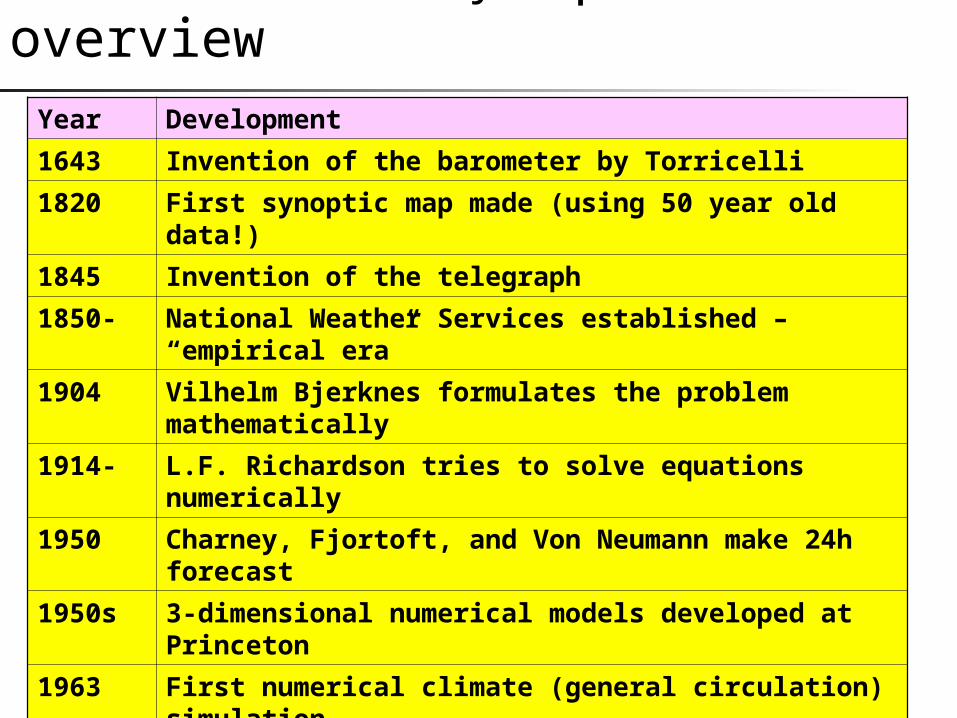
1.2 Brief history: quick overviewYear Development

1643 Invention of the barometer by Torricelli

1820 First synoptic map made (using 50 year old data!)

1845 Invention of the telegraph

1850- National Weather Services established – “empirical era”

1904 Vilhelm Bjerknes formulates the problem mathematically

1914- L.F. Richardson tries to solve equations numerically

1950 Charney, Fjortoft, and Von Neumann make 24h forecast

1950s 3-dimensional numerical models developed at Princeton

1963 First numerical climate (general circulation) simulation

1967 Global ocean model developed by Cox and Bryan

1970s Coupled models, spectral methods, and start of ECMWF

1980s Semi-lagrangian methods, data assimilation, etc.

1990s Massively parallel processors (MPPs), ensemble forecasts

2000s Earth system modelling …

14

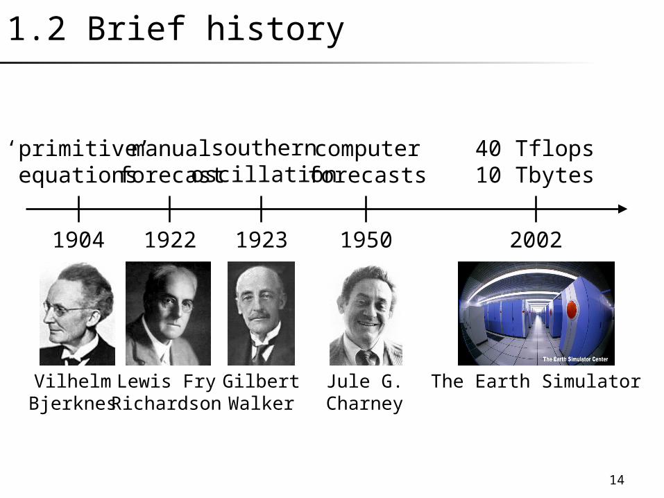
1.2 Brief history

Jule G.Charney

VilhelmBjerknes

The Earth SimulatorLewis FryRichardson

1950

computerforecasts

1922

manualforecast

‘primitive’equations

1904 2002

GilbertWalker

40 Tflops10 Tbytes

southernoscillation

1923

15

1.2 Brief history: Svante August Arrhenius (1859-1927)

Concern of effect on climate of doubling CO2

Arrhenius, S. 1896aUber den einfluss des atmosphaerischen kohlensauregehalts auf die temperatur der erdoberflaeche Proc. of the Royal Swedish Academy ofSciences 22.

Arrhenius, S. 1896bOn the influence of carbonic acid in the air upon the temperature of the ground,The London, Edinburgh, and Dublin PhilosophicalMagazine and Journal of Science, 41, 237-76.

16

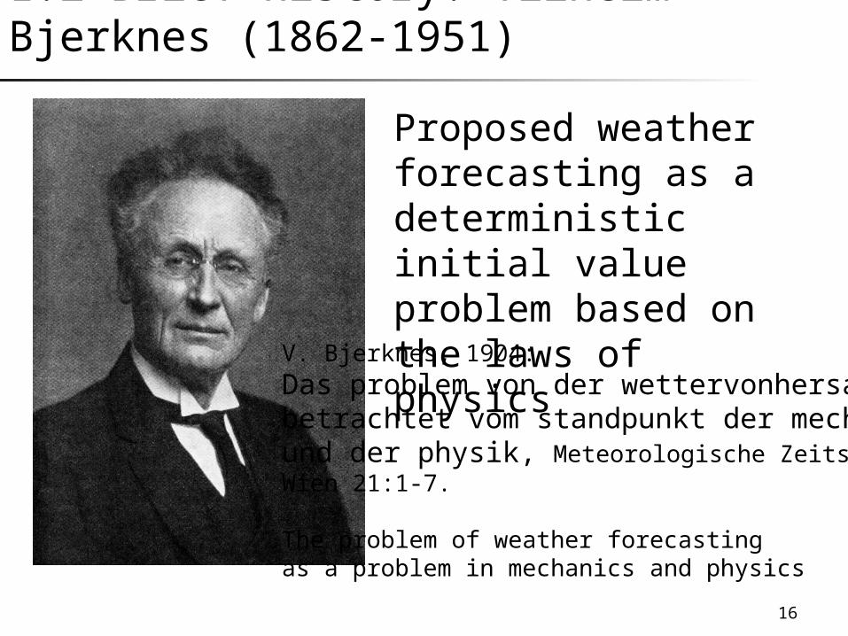
1.2 Brief history: Vilhelm Bjerknes (1862-1951)

Proposed weather forecasting as a deterministic initial value problem based on the laws of physics

V. Bjerknes, 1904:Das problem von der wettervonhersage, betrachtet vom standpunkt der mechanik und der physik, Meteorologische Zeitschrift, Wien 21:1-7.

The problem of weather forecasting as a problem in mechanics and physics

17

1.2 Brief history: The Bergen school

The Bergen Weather Service 14 Nov 1914

18

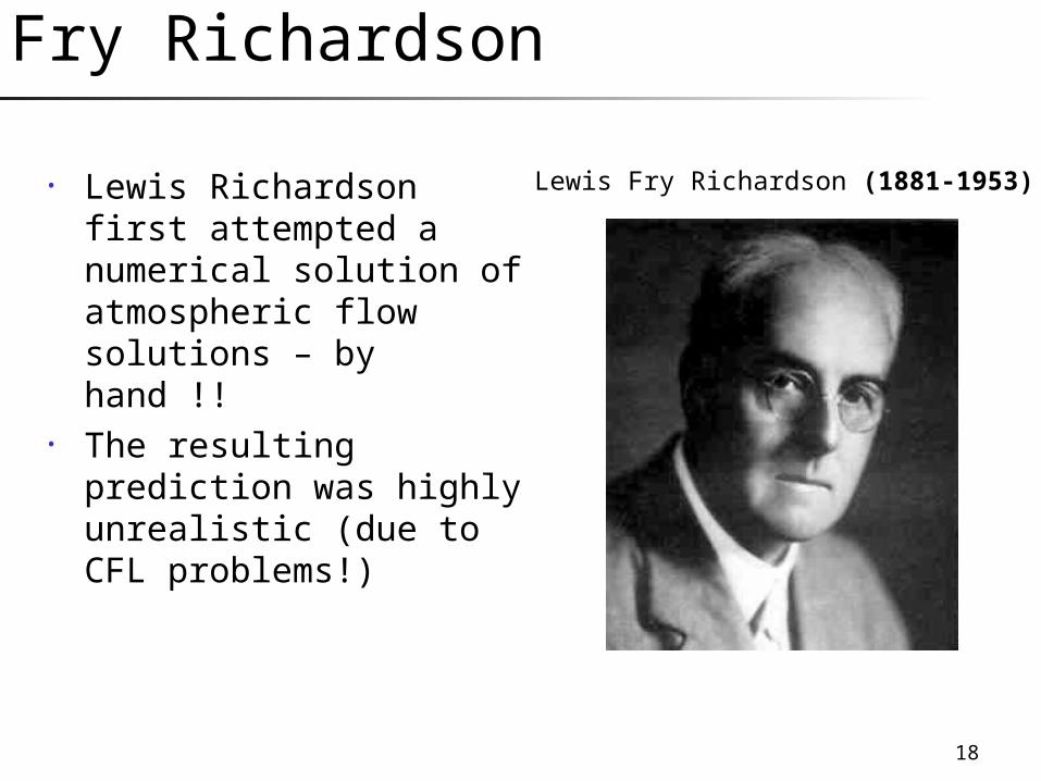
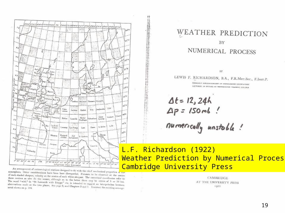
1.2 Brief history: Lewis Fry Richardson

• Lewis Richardson first attempted a numerical solution of atmospheric flow solutions – by hand !!

• The resulting prediction was highly unrealistic (due to CFL problems!)

Lewis Fry Richardson (1881-1953)

19

L.F. Richardson (1922) Weather Prediction by Numerical Process, Cambridge University Press

20

21

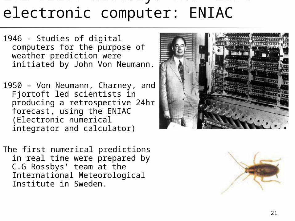
1.2 Brief history: The first electronic computer: ENIAC

1946 - Studies of digital computers for the purpose of weather prediction were initiated by John Von Neumann.

1950 – Von Neumann, Charney, and Fjortoft led scientists in producing a retrospective 24hr forecast, using the ENIAC (Electronic numerical integrator and calculator)

The first numerical predictions in real time were prepared by C.G Rossbys’ team at the International Meteorological Institute in Sweden.

22

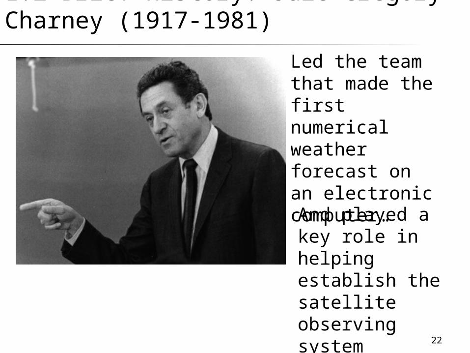
1.2 Brief history: Jule Gregory Charney (1917-1981)

Led the team that made the first numerical weather forecast on an electronic computer…

And played a key role in helping establish the satellite observing system

23

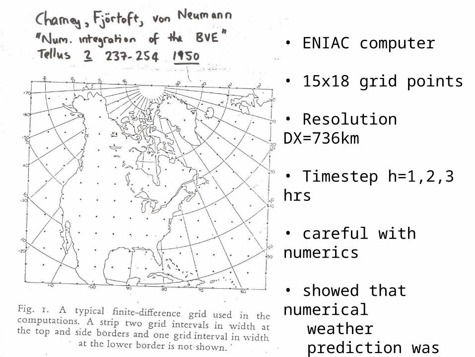
• ENIAC computer

• 15x18 grid points

• Resolution DX=736km

• Timestep h=1,2,3 hrs

• careful with numerics

• showed that numerical

weather prediction was feasible.

24

1.2 Brief history: Edward Lorenz (1917 – )

bZXYZ

YrXXZY

YXX

“… one flap of a sea-gull’s wing may forever change the future course of the weather” (Lorenz, 1963)

25

1.2 Brief history: Syukuro Manabe (1931-)

First predictions of global warming based on comprehensive global climate models

Smagorinsky, J., S. Manabe, J. L. Holloway, Jr., 1965:Numerical results from a nine-level general circulation model of the atmosphere. Monthly Weather Review, 93(12), 727-768.

Manabe, S., and R. T. Wetherald, 1975: The effects of doubling CO2 concentration on the climate of a general circulation model. Journal of the Atmospheric Sciences, 32(1), 3-15.

Manabe, S., K. Bryan, and M. J. Spelman, 1975: A global ocean-atmosphere climate model. Part I. The atmospheric circulation. Journal of Physical Oceanography, 5(1), 3-29.

26

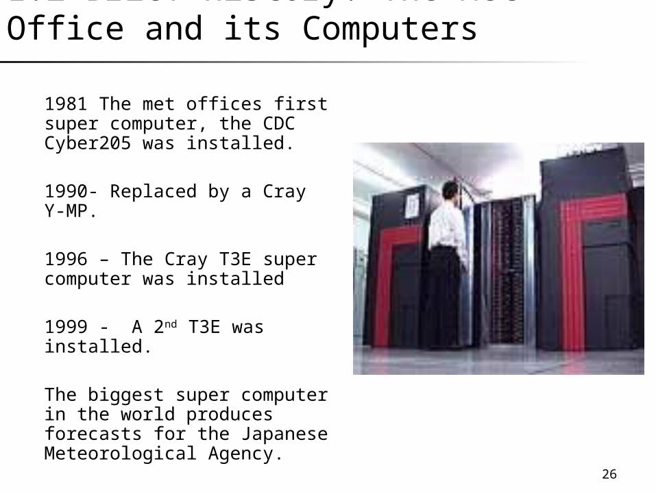
1.2 Brief history: The Met Office and its Computers

1981 The met offices first super computer, the CDC Cyber205 was installed.

1990- Replaced by a Cray Y-MP.

1996 – The Cray T3E super computer was installed

1999 - A 2nd T3E was installed.

The biggest super computer in the world produces forecasts for the Japanese Meteorological Agency.

27E x t r a 1 3H a d l e y C e n t r e f o r C l i m a t e P r e d i c t i o n a n d R e s e a r c h

V e r t i c a l e x c h a n g e b e t w e e n l a y e r so f m o m e n t u m , h e a t a n d m o i s t u r e

H o r i z o n t a l e x c h a n g eb e t w e e n c o l u m n so f m o m e n t u m , h e a t a n d m o i s t u r e

V e r t i c a l e x c h a n g eb e t w e e n l a y e r so f m o m e n t u m , h e a t a n d s a l t sb y d i f f u s i o n , c o n v e c t i o na n d u p w e l l i n g O r o g r a p h y , v e g e t a t i o n a n d s u r f a c e c h a r a c t e r i s t i c s

i n c l u d e d a t s u r f a c e o n e a c h g r i d b o x

V e r t i c a l e x c h a n g e b e t w e e n l a y e r sb y d i f f u s i o n a n d a d v e c t i o n

M o d e l l i n g G l o b a l C l i m a t e

1 5 ° W6 0 ° N

3 . 7 5 °

2 . 5 °

1 1 . 2 5 ° E4 7 . 5 ° N

28

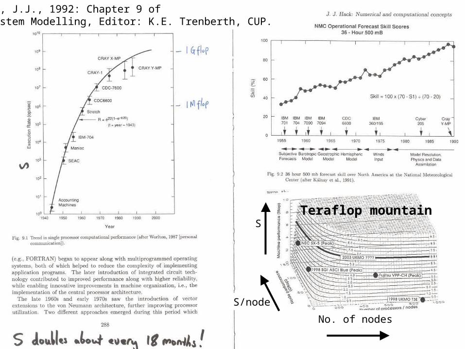
From: Hack, J.J., 1992: Chapter 9 ofClimate System Modelling, Editor: K.E. Trenberth, CUP.

No. of nodes

S

S/node

Teraflop mountain

29

Earth System Simulator - Japan

30

1.2 Brief history: Driving factors

Forecasting needs: Nowcasting (up to 6 hours lead) Short-range (6h-3days) Medium-range (3-10 days) Extended-range (10-30 days) Long-range (>30 days) – seasonal/climate forecasts

Computer technology – speed and memory

Availability of more data e.g. satellite measurements

31

32

1.3 Dynamical equations: hierarchies of models

Molecular dynamics – predict the motion of 1045 molecules using Newton’s laws (not feasible!)

Navier-Stokes equations – use the continuum approximation to treat gas as a continuous fluid. Includes sound, gravity, inertial, and Rossby waves.

Euler equations – use the incompressible or anelastic approximations to filter out sound waves that have little relevance to meteorology (speeds > 300m/s)

Primitive equations – use the hydrostatic approximation to filter out vertically propagating gravity waves (speeds >30m/s)

Shallow water equations – linearise about a basic steady flow in order to describe horizontal flow for different vertical modes. Each mode has a different equivalent depth external mode (e.g. tsunami) + barotropic mode + baroclinic modes

Vorticity equations – assume geostrophic balance to remove gravity waves. Useful in understanding extra-tropical dynamics.

More conceptual models: 0d (low order), 1d, and 2d models.

33

1.3 Waves in a compressible atmosphere

From J.S.A. Green dynamics notes

34

1.3 Some basic sets of equations

Primitive equations Shallow water eqns Barotropic vor. eqn

0log

0.

0

0

pDt

TD

pu

p

RT

p

ufzDt

Du

p

p

0

0

0

y

v

x

ugH

t

yfu

t

vx

fvt

u0 v

Dt

D

Exercise: Derive prognostic equations for relative vorticity and divergence using the shallow water equations and compare the resultingvorticity equation to the barotropic vorticity equation.

35

1.3 Dynamical systems theory

],;[][ tFQt

is a multidimensional state vector

The state of the system can be represented by a pointin state space.

Movement of point (flow) in state space representsthe evolution of the system

Q is hydrodynamical advection term (dynamical core)F is forcing and dissipation due to physical processes

36

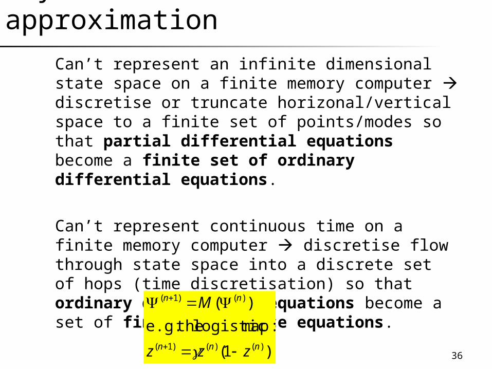
Why we need numerical approximation

Can’t represent an infinite dimensional state space on a finite memory computer discretise or truncate horizonal/vertical space to a finite set of points/modes so that partial differential equations become a finite set of ordinary differential equations.

Can’t represent continuous time on a finite memory computer discretise flow through state space into a discrete set of hops (time discretisation) so that ordinary differential equations become a set of finite difference equations.

)1(

:map logistic thee.g.

)(

)()()1(

)()1(

nnn

nn

zzz

M

37

1.3 Finite difference methods in time & space

Idea: Replace all derivatives by finite difference approximations:

For example: 0

xu

t

02

)(

2

)( )(1

)(1

)1()1(

nj

njn

i

nj

nj u

h

Centered Time Centred Space (CTCS)n=“time level” j=“grid point”h=“time step” delta=“grid spacing”

1-dimensional advection equation

),(),()( nhjtx njnj

38

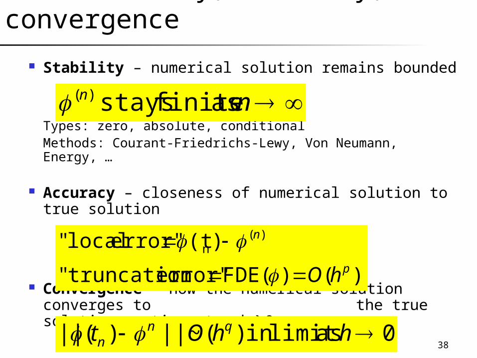
1.3 Stability, accuracy, and convergence

Stability – numerical solution remains bounded

Types: zero, absolute, conditionalMethods: Courant-Friedrichs-Lewy, Von Neumann, Energy, …

Accuracy – closeness of numerical solution to true solution

Convergence – how the numerical solution converges to the true solution as time step h0

nn as finite stays )(

)()FDE( error" truncation"

)(t error" local" )(n

p

n

hO

0 aslimit in )(||~)(|| hhOt qnn

39

1.3 Numerical instability

So stable & consistent (p>=1 accurate) linear schemes converge on the true solution as h0. E.g. stable 2nd order leapfrog schemes.

Lax equivalence theorem:A stable p’th order accurate

linear finite difference equation

is p’th order convergent

Numerical solutions that growexponentially with time step

40

1.3 Courant-Friedrichs-Lewy stability analysis (CFL)

R. Courant, K.O. Friedrichs, and H. Lewy, 1928: Uber die partiellen Differen-zengleichungen der mathematischen Physik. Mathematische Annalen, Vol. 100, pages 32-74.

Domain of dependence of the finite difference scheme must

include the domain of dependence of the partial differential equation. (necessary but not sufficient condition for stability)

dh

Example:FDE of advection eqn.where the value on the next time stepdepends on nearest neigbour values.

41

1.3 Implications of CFL

Information should not spread more than one grid spacing in one time step (for a FTCS advection scheme!)

Time step needs to be small enough to avoid instability caused by the fastest waves e.g. h<d/c fast waves require lots of time steps & computer time! filter out fastest waves, slow down waves, move grid with the flow

Note that c is the “phase velocity” simulated by the finite difference equations and so methods that can slow down unwanted fast waves can be used to avoid CFL.

Diffusion and advection can also cause CFL instability!

42

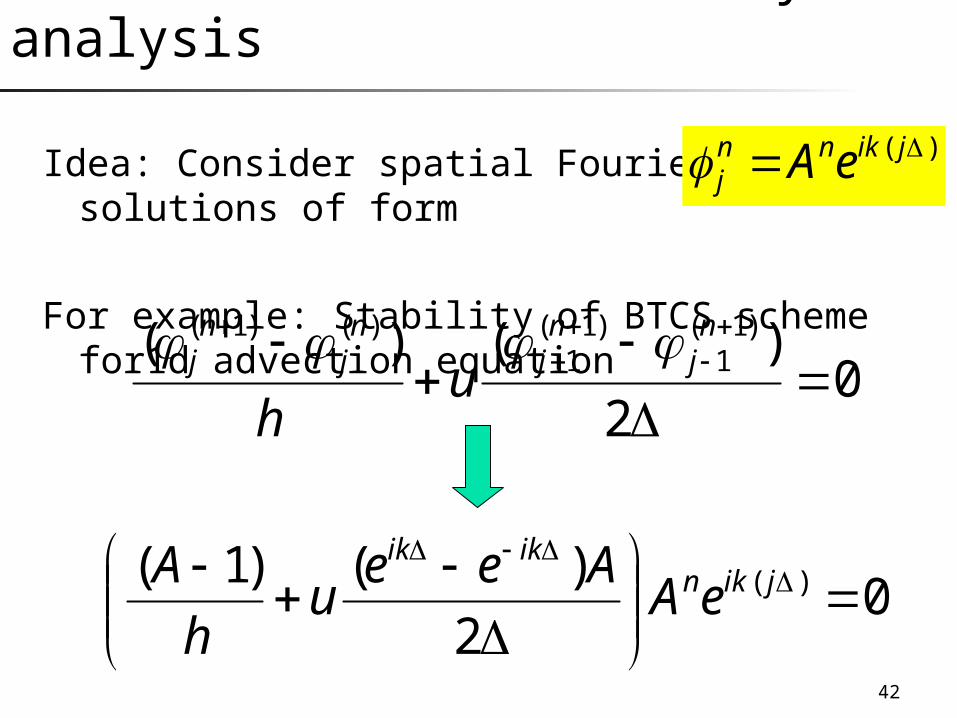
1.3 Von Neumann stability analysis

Idea: Consider spatial Fourier solutions of form

For example: Stability of BTCS scheme for1d advection equation

02

)()( )1(1

)1(1

)()1(

nj

nj

nj

nj u

h

)( jiknnj eA

02

)()1( )(

jiknikik

eAAee

uh

A

43

1.3 Von Neumann stability analysis

dispersion relation

Dependence of angular frequency on wavenumber

ieAkiuh

A

1

sin1

02

)()1( )(

jiknikik

eAAee

uh

A

(damped) stable always 1sin11

22

222

khu

A

kuh

ckhh sintan 1

44

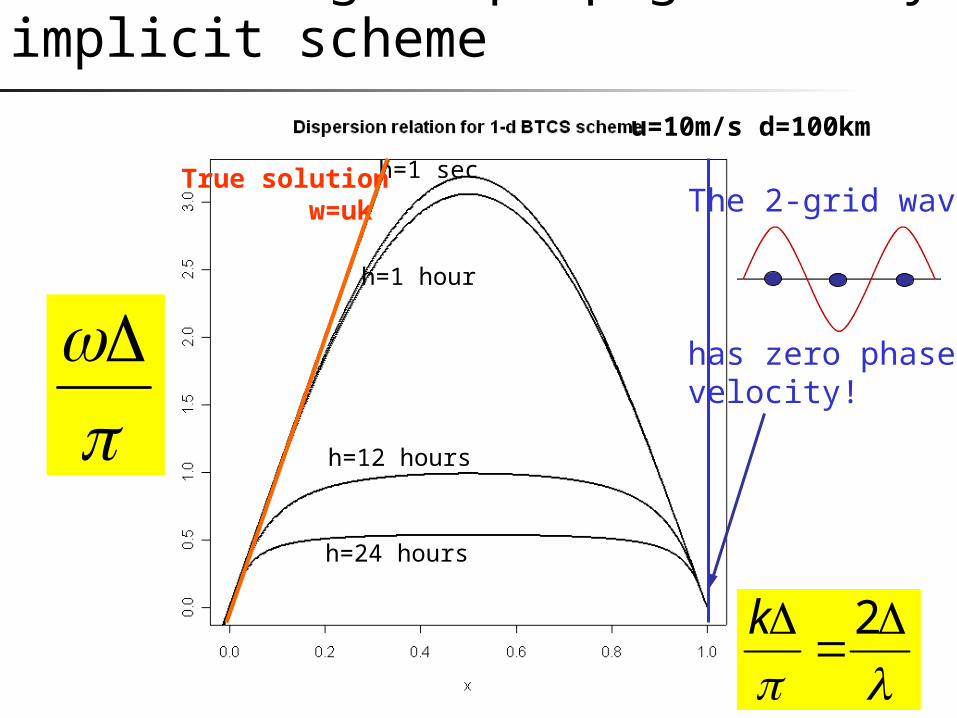
1.3 Slowing of propagation by implicit scheme

h=1 sec

h=1 hour

h=12 hours

h=24 hours

True solutionw=uk

2k

The 2-grid wave

has zero phasevelocity!

u=10m/s d=100km

45

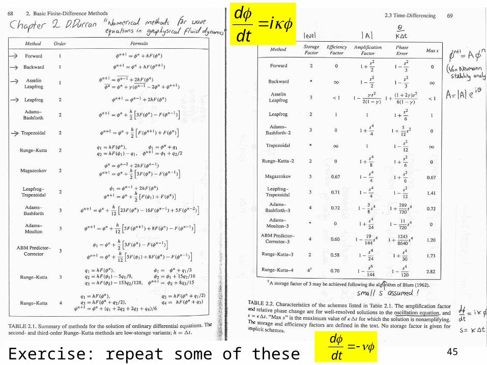
i

dt

d

Exercise: repeat some of these calculations but for

dt

d

46

1.3 Summary of main points

Weather prediction and climate simulation is limited by the amount of computer time available

Stability, accuracy and speed are the main concerns when developing numerical schemes

CFL stability analysis shows that higher spatial resolution simulations require smaller time steps

Methods have been developed to filter out fast waves (e.g. sound waves, v.prop gravity waves) slow down fast waves (e.g. semi-implicit schemes) treat fast advection by moving with the flow (semi-lagrangian)

47