Embed Size (px)
Citation preview

ESSAYS IN MACROECONOMICS AND DYNAMIC FACTOR MODELS
By
Ziyi Guo
Dissertation
Submitted to the Faculty of the
Graduate School of Vanderbilt University
in partial ful�llment of the requirements
for the degree of
DOCTOR OF PHILOSOPHY
in
Economics
August, 2013
Nashville, Tennessee
Approved:
Professor Mototsugu Shintani
Professor Mario J. Crucini
Professor Kevin X.D. Huang
Professor David C. Parsley

Copyright c 2013 by Ziyi Guo
All Rights Reserved

To my parents and my old sister of whose lives I am proud.
ii

ACKNOWLEDGMENTS
I am especially grateful to my advisor Dr. Mototsugu Shintani, who gives me
tremendous guidance and support on this and many other research. I cannot thank him
enough for the countless discussions and insights he has passed on to me. I also especially
thank my committe members - Dr. Mario J. Crucini, Dr. Kevin X.D. Huang and Dr. David
C. Parsley for their valuable comments and useful discussions.
I also have been bene�ted from the insightful comments from my presentations at
Vanderbilt University, the 2012 Midwest Macroeconomics Meetings at University of Notre
Dame and the 2012 Midwest Econometrics Meetings at University of Kentucky. In particu-
lar, I thank Dr. Chris Benett, Eric Bond, William Collins, Yanqin Fan, Gregory Hu¤man,
Tong Li, Jingfeng Lu, and Joel Rodrigue.
This work has been generously supported by College of Arts & Sciences Sum-
mer Research Award, Kirk Dornbush Summer Research Grant, and Graduate Research
Assistantship at Vanderbilt University. Without these �nancial supports, this work would
not have been possible. Also, without the professional assistance provided by Ms. Kathleen
Finn, this work cannot be completed.
I am also grateful for all of the classmates and o¢ cemates who have made my years
in graduate school a great experience. I am looking forward to interacting and working with
many of these friends and colleagues in the future.
Finally, I would like to thank my parents, Turen Guo and Xinv Chen, as well as
my old sister, Nina Guo, for their endless love and unconditional encouragement throughout
my life. Without their support, I could not �nish my degree in the end.
iii

TABLE OF CONTENTS
Page
ACKNOWLEDGMENTS ........................................................................................ iii
LIST OF TABLES.................................................................................................. vi
LIST OF FIGURES................................................................................................ vii
Chapter
I NOISY INFORMATION IN AN INTERNATIONAL REAL BUSINESS CYCLEMODEL .......................................................................................................... 1
Introduction............................................................................................... 1
Model........................................................................................................ 4Firms.............................................................................................. 5Households...................................................................................... 6Equilibrium..................................................................................... 8
Implications for International Business Cycles .............................................. 9International Output Correlation (� = �� = 0) .................................. 9International Consumption Correlation (� = �� > 0).......................... 13International Productivity-Hours Dynamics (� 6= ��) ......................... 15
The Model with Capital Accumulation ........................................................ 16
Conclusion ................................................................................................. 18
Appendix A ............................................................................................... 20
Appendix B ............................................................................................... 27
Appendix C ............................................................................................... 31
II FINITE SAMPLE PERFORMANCE OF PRINCIPAL COMPONENTS ESTI-MATORS FOR DYNAMIC FACTOR MODELS: ASYMPTOTIC AND BOOT-STRAP APPROXIMATIONS ........................................................................... 40
Introduction............................................................................................... 40
Two-Step Estimation of the Autoregressive Model of Latent Factor............... 43
The Bootstrap Approach to Bias Correction ................................................ 50
The Bootstrap Approach to Con�dence Intervals.......................................... 53
Empirical Application to US Di¤usion Index................................................ 56
Conclusion ................................................................................................. 57
III INFORMATION HETEROGENEITY, HOUSING DYNAMICS AND THE BUSI-NESS CYCLE ................................................................................................. 88
Introduction............................................................................................... 88
Empirical Motivation.................................................................................. 93
The Basic Model ........................................................................................ 96Entrepreneurs.................................................................................. 97Households...................................................................................... 98
iv

Market Clearing .............................................................................. 99Shocks ............................................................................................ 100The Information Structure and the Equilibrium................................. 100
Economic Implications................................................................................ 101What drives house prices �uctuations?.............................................. 104Implications for Investment Dynamics............................................... 106
Empirical Evidence from Survey Data ......................................................... 108
Conclude ................................................................................................... 110
Appendix: Solving a DSGE model with heterogeneous information ............... 112
BIBLIOGRAPHY .................................................................................................. 119
v

vi
LIST OF TABLES Table Page 1 AR Estimation . . . . . . . . . . . . . . . . . . . . . . . . . . . . . . . . . . . . . . . . . . . . . . . . . . . . . . . . . . . . . 81 2 Two-Step AR Estimation . . . . . . . . . . . . . . . . . . . . . . . . . . . . . . . . . . . . . . . . . . . . . . . . . . . . . 81 3 Bootstrap Bias Corrections . . . . . . . . . . . . . . . . . . . . . . . . . . . . . . . . . . . . . . . . . . . . . . . . . . . 82 4 Coverage Rate of Bootstrap Confidence Intervals . . . . . . . . . . . . . . .. . . . . . . . . . . . . . . . . . . 84 5 AR(1) Estimates of the US Diffusion Index . . . . . . . . . . . . . . . . . . . . . . . . . . . . . . . . . . . . . . 85 6 House Price Appreciation and Rental Prices . . . . . . . . . . . . . . . . . . . . . . . . . . . . . . . . . . . . . 113 7 Second Moments – Empirical Lead-Lag Correlations. . . . . . . . . . . . . . . . . . . . . . . . . . . . . . 113 8 The Causality Test between Residential and Business Investments . . . . . . . . . . . . . . . . . . . 113 9 Business Cycle Statistics for the Models. . . . . . . . . . . . . . . . . . . . . . . . . . . . . . . . . . . . . . . . 114 10 House Price Appreciation and Rental Prices in Simulated Data . . . . . . . . . . . . . . . . . . . . . . 114
vii
LIST OF FIGURES Figure Page 1 The Correlations of Outputs in Different Asset Markets. . . . . . . . . . . . . . . . . . . . . . . . . . . . . 34 2 The Impulse Response of Consumption. . . . . . . . . . . . . . . . . . . . . . . . . . . . . . . . . . . . . . . . . . 34 3 Outputs Growth Correlation and Consumption Growth Correlation with Different Degrees of
Noise Shocks ( 0.6κ κ =*= ) . . . . . . . . . . . . . . . . . . . . . . . . . . . . . . . . . . . . . . . . . . . . . . . . . 35
4 Labor Productivity and Hours Worked during the Recent Financial Crisis . . . . . . . . . . . . . . 36 5 The Correlations of Hours Worked Growth . . . . . . . . . . . . . . . . . . . . . . . . . . . . . . . . . . . . . . 37
6 Productivity Growth and Hours Growth Correlation ( *0.1 and 0.7κ κ= = ). . . . . . . . . . . 37
7 The Correlations of Outputs in Different Asset Markets (Models with Capital). . . . . . . . . . . 38 8 Outputs Growth Correlation and Consumption Growth Correlation with Different Degrees of
Noise Shocks (Models with Capital, 0.7κ κ =*= ). . . . . . . . . . . . . . . . . . . . . . . . . . . . . . . . 38
9 The Correlations of Hours Worked Growth (Models with Capital). . . . . . . . . . . . . . . . . . . . . 39 10 Productivity Growth and Hours Growth Correlation (Models with Capital, 0.1 κ = and
0.7κ = ) . . . . . . . . . . . . . . . . . . . . . . . . . . . . . . . . . . . . . . . . . . . . . . . . . . . . . . . . . . . . . . . . . 39 11 US Diffusion Index . . . . . . . . . . . . . . . . . . . . . . . . . . . . . . . . . . . . . . . . . . . . . . . . . . . . . . . . . 86 12 Home Rents and House Prices with the Business Cycle . . . . . . . . . . . . . . . . . . . . . . . . . . . . 115 13 Residential Investment and Nonresidential Investment with the Business Cycle . . . . . . . . . 115 14 House Prices in Response to TFP Shocks . . . . . . . . . . . . . . . . . . . . . . . . . . . . . . . . . . . . . . . 116 15 Average Expectation of Next-Period House Prices . . . . . . . . . . . . . . . . . . . . . . . . . . . . . . . . 116

viii
16 Empirical Evidences from SVAR. . . . . . . . . . . . . . . . . . . . . . . . . . . . . . . . . . . . . . . . . . . . . . 117 17 Simulation Evidences from SVAR. . . . . . . . . . . . . . . . . . . . . . . . . . . . . . . . . . . . . . . . . . . . . 117

CHAPTER I
NOISY INFORMATION IN AN INTERNATIONAL REAL BUSINESS CYCLE MODEL
Introduction
Standard international real business cycle (IRBC) models formulated by Backus,
Kehoe, and Kydland (BKK, 1992, 1995) have been considered a natural starting point to
assess the quantitative implications of dynamic stochastic general equilibrium (DSGE) mod-
els in an open economy environment. Since the standard IRBC model under assumptions
of �exible prices and perfect competition cannot replicate all the observed characteristics
of international business cycles, a number of extended models with more realistic features
have been developed in the past two decades. Most importantly, incorporating monopolis-
tic competition and sticky prices, along with the monetary sector in open economy DSGE
models has been proven to be very successful in matching the data. In contrast to a large
interest in the role of nominal rigidities, however, few studies have attempted to formally
assess the quantitative implications of introducing informational frictions in the model.
In this paper, we introduce a noisy information structure in an otherwise standard IRBC
model and show that an extension in this direction is also useful in understanding some key
features of international comovements of output, consumption, and labor.
We consider an imperfect information variant of a standard two-country bond-
economy IRBC model similar to the one used in Baxter and Crucini (1995) and Heathcote
and Perri (2002), except that we exclude capital accumulation from the model. While we
believe that an open economy DSGE model with nominal rigidities is more realistic, we
maintain the assumptions of perfect competition and �exible prices in this paper simply
because they provide a reasonable benchmark in evaluating the pure e¤ect of imperfect
1

information on the international business cycle properties. In terms of explaining the in-
ternational comovement, the original BKK model predicts negative (or near-zero) output
correlation, near-perfect consumption correlation, and negative correlation of factors of pro-
duction, all of which contradict the data. To improve the performance of the model, Baxter
and Crucini (1995) and Kollman (1996) replaced the complete market assumption of the
BKK model with the incomplete market assumption, so that consumers only have access
to a real bond market. A convenient approach to ensure a unique stationary solution to an
open economy model of incomplete market is to impose a (small) real cost of bond holding
(see Heathcote and Perri, 2002, and Schmitt-Grohe and Uribe, 2003). According to the
simulation results reported by Boileau and Normandin (2008, Table 1), under the station-
ary technology process with positive international spillovers, an incomplete market model
with a tiny bond holding cost can yield positive international output correlation, but its
magnitude is still less than the data.1 As in the original BKK model, we focus on station-
ary technology shocks with international spillovers as a source of aggregate �uctuations.
However, domestic �rms are assumed to observe the current foreign technology with noise.
We �rst show that when the information noise is su¢ ciently large, the model can match
the positive output comovement in the data not only for the case of incomplete market but
also for the case of perfect international risk sharing.
Even in the case of incomplete market where international consumption risk shar-
ing is restricted, the standard IRBC models with stationary technology shocks are known
to predict international consumption correlation higher than the international output cor-
relation (see Boileau and Normandin, 2008, Table 1). The data, however, typically suggest
that the former is lower than the latter (see Ambler, Cardia, and Zimmermann, 2004).
To narrow the gap between output correlation and consumption correlation predicted by
the model, several di¤erent channels have been emphasized in the literature. For example,
1Baxter and Crucini (1995) emphasized the better performance of the bond economy model when thetechnology is highly persistent and there is no international spillover.
2

the proposed channels include nontraded goods (Stockman and Tesar, 1995), endogenous
incomplete market with limited enforcement (Kehoe and Perri, 2002), sticky prices (Chari,
Kehoe, and McGrattan, 2002) and variable capital utilization (Baxter and Farr, 2005). In
this paper, we highlight the information channel and show that the presence of a noisy
information structure in the household sector helps to �ll the gap between the cross country
output correlation and consumption correlation.
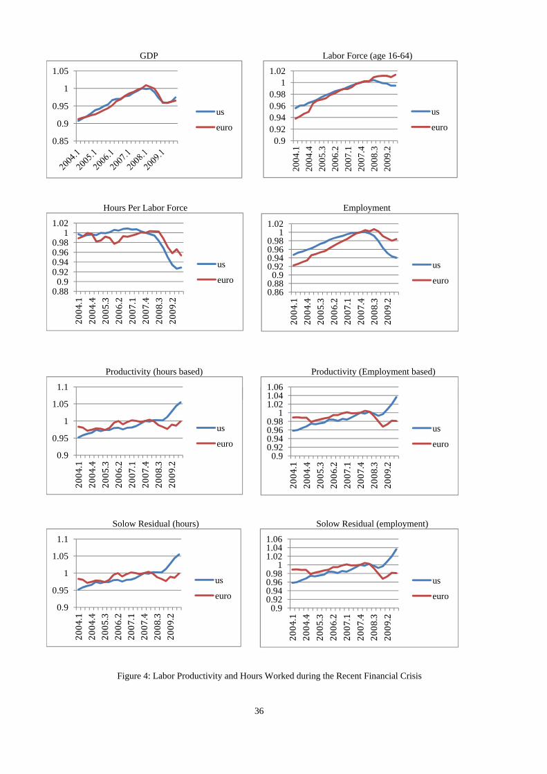
In the recent global �nancial crisis of 2007-2009, employment and hours worked
declined both in the US and Euro area. Such a positive comovement is not predicted
by the standard IRBC models but can be generated in our imperfect information variant
of the model. Furthermore, since the labor declined more in the US than in the Euro
area, observed labor productivity increased in the US, which contrasts to the Euro area
where near-zero or negative productivity growth was observed. The empirical observation
of near-zero (or negative) correlation between productivity and hours worked has been
viewed as a productivity-hours anomaly in the macroeconomic literature, since the standard
real business cycle models predict positive response of hours worked to positive technology
shocks, provided an upward sloping labor supply curve (see for example, Galí, 1999, and
Christiano, Eichenbaum, and Vigfusson, 2003). To explain the negative productivity-hours
correlation, Galí (1999) emphasizes the role of monetary policy shocks and sticky prices. In
this paper, we show that negative productivity-hours correlation can also be predicted from
the noisy information structure even if prices are �exible and that heterogenous observations
in two regions can be obtained if the fraction of information-constrained consumers di¤ers
across regions.
We note that there are other studies that emphasize the role of imperfect in-
formation structures in open economy macroeconomic models. For example, Gourinchas
and Tornell (2004) discuss distorted beliefs of investors, while Bacchetta and van Wincoop
(2006) and Crucini, Shintani, and Tsuruga (2010), respectively, introduce the heterogenous
3

information and sticky information structures in open economy monetary models. However,
these studies mainly focus on explaining nominal and real exchange rate dynamics rather
than the international comovement of real variables. Luo, Nie, and Young (2010) introduce
the rational inattention to an intertemporal current account model. However, since the
intertemporal current account model is a small open partial equilibrium model, it is not
suitable for understanding cross-country correlations. In our paper, we introduce a noisy
information structure in a two-country economy general equilibrium model with direct im-
plications on cross-country comovements. Our approach is similar in spirit to Angeletos and
La�O (2009), who introduce an imperfect common knowledge structure in a close-economy
real business cycle model and show that the model can induce a negative short-run response
of employment to productivity shocks. Unlike their model where heterogenous information
across �rms plays an important role, we assume homogeneous information across �rms but
only allow heterogenous information between countries. Even with such a simple informa-
tion structure, the model still has rich implications on international business cycle features.
The remainder of the paper is organized as follows. Our two-country model with
noisy information is introduced in Section 2. Section 3 discusses the implications of our
model on output, consumption and labor in order. Section 4 extends the baseline model
with capital accumulation. Section 5 concludes.
Model
Our baseline international real business model is a simpli�ed version of the two-
country bond-economy model of Baxter and Crucini (1995) from which we have eliminated
capital accumulation. We introduce information noise to both �rms and households in
the baseline model and compare it with the case of perfect information. Foreign country
4
variables are denoted by stars.
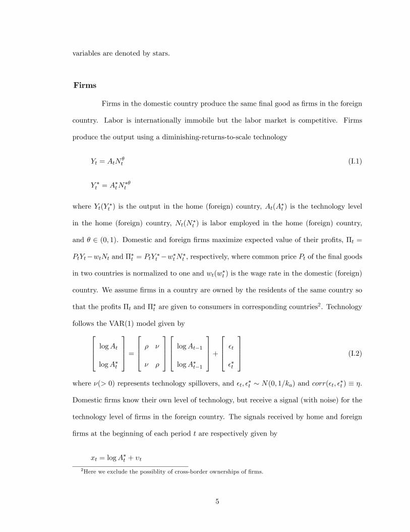
Firms
Firms in the domestic country produce the same �nal good as �rms in the foreign
country. Labor is internationally immobile but the labor market is competitive. Firms
produce the output using a diminishing-returns-to-scale technology
Yt = AtN�t (I.1)
Y �t = A�tN��t
where Yt(Y �t ) is the output in the home (foreign) country, At(A�t ) is the technology level
in the home (foreign) country, Nt(N�t ) is labor employed in the home (foreign) country,
and � 2 (0; 1). Domestic and foreign �rms maximize expected value of their pro�ts, �t =
PtYt�wtNt and ��t = PtY�t �w�tN�
t , respectively, where common price Pt of the �nal goods
in two countries is normalized to one and wt(w�t ) is the wage rate in the domestic (foreign)
country. We assume �rms in a country are owned by the residents of the same country so
that the pro�ts �t and ��t are given to consumers in corresponding countries2. Technology
follows the VAR(1) model given by2664 logAt
logA�t
3775 =2664 � �
� �
37752664 logAt�1logA�t�1
3775+2664 �t
��t
3775 (I.2)
where �(> 0) represents technology spillovers, and �t; ��t � N(0; 1=ka) and corr(�t; ��t ) � �.
Domestic �rms know their own level of technology, but receive a signal (with noise) for the
technology level of �rms in the foreign country. The signals received by home and foreign
�rms at the beginning of each period t are respectively given by
xt = logA�t + �t
2Here we exclude the possiblity of cross-border ownerships of �rms.
5

and
x�t = logAt + ��t
where �t; ��t � N(0; 1=kx).
Households
Each country consists of two types of consumers. The �rst type (type 1) decides
the consumption level based on the same information set as the �rms located in the same
country. The fraction of the type 1 consumers in the home (foreign) country is represented
by �(��). The remaining consumers choose their consumption level after the information on
the foreign technology level is revealed. Households consume the �nal products and supply
labor to �rms located in the same country. Each type of consumer in the home country
maximizes the expected value of the discounted sum of utility given by
1Xt=0
�t[C1� it
1� �N1+�it
1 + �]
conditional on the information available at the decision timing, where Cit and Nit are
consumption and labor supply of type i (i = 1; 2) consumers, (� 0) is the reciprocal of the
intertemporal elasticity of substitution or relative risk aversion, �(� 0) is the reciprocal of
the Frisch elasticity of labor supply, and � is the discount factor. The international asset
market is restricted to trade only non-contingent bonds. The household budget constraint
is given by
Cit +QtBit+1 +�
2B2it+1 � �t + wtNit +Bit
where Bit is bonds held by the type i consumers, Qt (= (1 + rt)�1) is the price of bonds
in units of good, rt is the world interest rate, and (�=2)B2it+1 is a quadratic holding cost of
6

bonds with � being a small positive value. The household maximization problem is similarly
de�ned for foreign consumers with preferences identical to domestic consumers.
For the timing of decisions made by �rms and households, we follow the setting
of Angeletos and La�O (2009) and consider each period in two stages. At the beginning
of each time period (stage 1), �rms and labor representatives of households meet and de-
cide the production level based on the information set flogAt; xtg [ t�1. All households
make labor supply decisions at this stage. The type 1 consumers, � fraction of house-
holds, also determine their consumption level (which cannot be adjusted in the next stage).
Firms produce �nal goods. Then, at the end of each time period (stage 2), information
on foreign productivity is revealed. The type 2 consumers, the remaining 1� � fraction of
households, make their consumption-saving decisions based on the updated information set
t = flogAt; logA�t ; xt; x�t g [ t�1. The interest rate level and the real wage rate level are
determined where the bond market and the labor market clear. Countries export or import
goods in the world market.
Reis (2006) built a microfoundation of inattentive consumers, who update their
information sporadically. Mankiw and Reis (2006) further considered the role of inattentive
consumers in a general equilibrium framework. In our model, type 1 consumers play a role
similar to that of inattentive consumers (planner) considered in Mankiw and Reis (2006),
except that we allow our consumers to observe a signal. The presence of type 2 consumers,
who make their consumption decision after all the information is revealed, is essential in
closing our model so that � = 1 case is excluded in the analysis. The timing of the decision
made by type 2 consumers is important in avoiding strategic responses by �rms and type 1
consumers. In the beginning of each period, neither �rms nor type 1 consumers can observe
prices to extract the information about the state of the economy. Since there is no strategic
responses by �rms, they make their production decisions based on their expected value of
the price, conditional on their restricted information set. Likewise, type 1 consumers make
7

their saving-borrowing decisions based on their conditional expectation of the interest rate.
Equilibrium
Labor is internationally immobile so that the labor market clearing condition for
each country is respectively given by
Nt = �N1t + (1� �)N2t
and
N�t = ��N�
1t + (1� ��)N�2t
Trade across countries is allowed so that the world goods-market clearing condition (resource
constraint) is given by
Yt � Ct + Y �t � C�t ���
2B21t+1 �
���
2B�21t+1 �
(1� �)�2
B22t+1 �(1� ��)�
2B�22t+1 = 0
where
Ct = �C1t + (1� �)C2t
and
C�t = ��C�1t + (1� ��)C�2t:
Finally, the Walras�Law implies that the remaining bond market clears as
�B1t + ��B�1t + (1� �)B2t + (1� ��)B�2t = 0
so that bonds are in zero net supply at the world level.
8

Implications for International Business Cycles
International Output Correlation (� = �� = 0)
We �rst solve the model and investigate its implication on the international output
correlation when � = �� = 0 so that all the consumers can decide their consumption levels
after the information about foreign technology is revealed. This setting is convenient for
comparing the implication of the model under incomplete market assumption and that of
the model under complete market assumption. To solve the model, we log-linearize all the
�rst-order conditions and then use the guess-veri�cation approach. That is, we assume a
policy function to take a linear form and plug it into the model to match the coe¢ cients of
the same state variables in the two sides of the equations.
Let yt = log Yt� log Y (y�t = log Y�t � log Y �) and bt = Bt=Y (b�t = B�t =Y
�) where
variables with no subscript imply steady state values. We then have the following results
on the level of output.
Proposition 1 Suppose � = �� = 0 under the incomplete market assumption. Then, (i)the equilibrium level of output in the home country and in the foreign country is given by
yt = m�1 logAt�1 +m��1 logA
�t�1 +m logAt +mxxt +mbbt (I.3)
y�t = m�1 logA�t�1 +m
��1 logAt�1 +m logA
�t +mxx
�t +mbb
�t
for some coe¢ cients (m�1;m��1;m;mx;mb); and
(ii) the equilibrium value of the coe¢ cients (m�1;m��1;m;mx;mb) satis�es the
following properties: m�1 and m��1 approach zero as ka=kx ! 0; m approaches a positive
value as ka=kx ! 0; mx approaches a negative value as ka=kx ! 0 and approaches zero askz=kx !1; and mb is invariant to ka=kx.
To illustrate the reason why the model with noisy information provides a quantita-
tively di¤erent result on international output correlation from the full information model, it
is helpful to �rst consider the case of the complete market which has a closed form solution.
For the complete market case, �rms�problems are the same as before but the households
9
maximize expected value of
1Xt=0
�tfC1� t
1� �N1+�t
1 + �+C�1� t
1� �N�1+�t
1 + �g
which is common across countries subject to the world resource constraint
Yt � Ct + Y �t � C�t = 0:
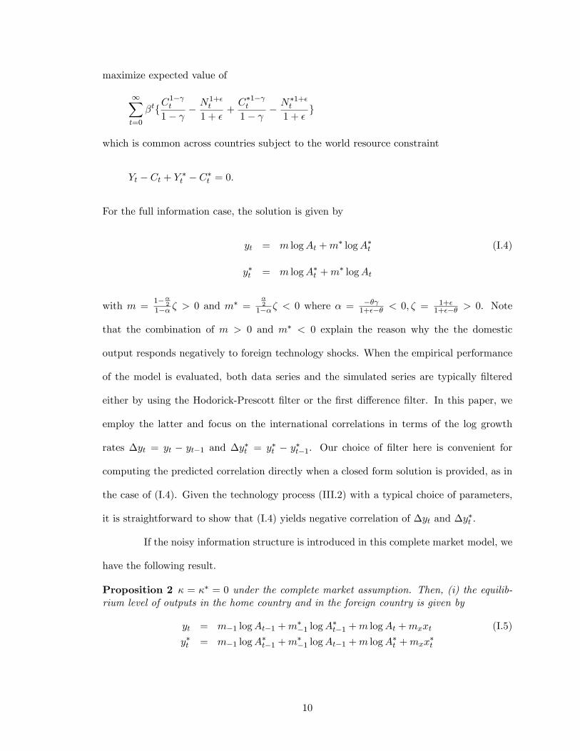
For the full information case, the solution is given by
yt = m logAt +m� logA�t (I.4)
y�t = m logA�t +m� logAt
with m =1��
21�� � > 0 and m� =
�2
1��� < 0 where � = �� 1+��� < 0; � = 1+�
1+��� > 0. Note
that the combination of m > 0 and m� < 0 explain the reason why the the domestic
output responds negatively to foreign technology shocks. When the empirical performance
of the model is evaluated, both data series and the simulated series are typically �ltered
either by using the Hodorick-Prescott �lter or the �rst di¤erence �lter. In this paper, we
employ the latter and focus on the international correlations in terms of the log growth
rates �yt = yt � yt�1 and �y�t = y�t � y�t�1. Our choice of �lter here is convenient for
computing the predicted correlation directly when a closed form solution is provided, as in
the case of (I.4). Given the technology process (III.2) with a typical choice of parameters,
it is straightforward to show that (I.4) yields negative correlation of �yt and �y�t .
If the noisy information structure is introduced in this complete market model, we
have the following result.
Proposition 2 � = �� = 0 under the complete market assumption. Then, (i) the equilib-rium level of outputs in the home country and in the foreign country is given by
yt = m�1 logAt�1 +m��1 logA
�t�1 +m logAt +mxxt (I.5)
y�t = m�1 logA�t�1 +m
��1 logAt�1 +m logA
�t +mxx
�t
10
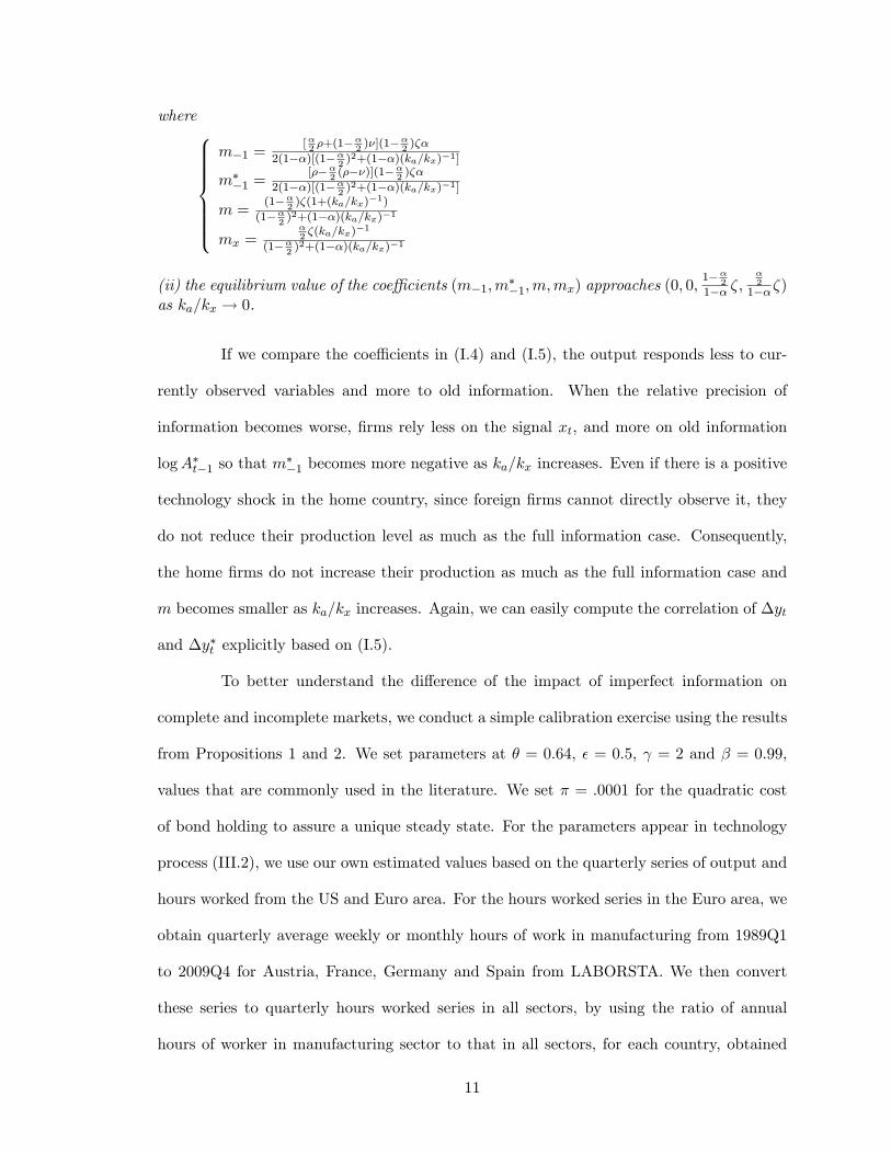
where8>>>>>><>>>>>>:
m�1 =[�2�+(1��
2)�](1��
2)��
2(1��)[(1��2)2+(1��)(ka=kx)�1]
m��1 =
[���2(���)](1��
2)��
2(1��)[(1��2)2+(1��)(ka=kx)�1]
m =(1��
2)�(1+(ka=kx)�1)
(1��2)2+(1��)(ka=kx)�1
mx =�2�(ka=kx)�1
(1��2)2+(1��)(ka=kx)�1
(ii) the equilibrium value of the coe¢ cients (m�1;m��1;m;mx) approaches (0; 0;
1��2
1�� �;�2
1���)as ka=kx ! 0.
If we compare the coe¢ cients in (I.4) and (I.5), the output responds less to cur-
rently observed variables and more to old information. When the relative precision of
information becomes worse, �rms rely less on the signal xt, and more on old information
logA�t�1 so that m��1 becomes more negative as ka=kx increases. Even if there is a positive
technology shock in the home country, since foreign �rms cannot directly observe it, they
do not reduce their production level as much as the full information case. Consequently,
the home �rms do not increase their production as much as the full information case and
m becomes smaller as ka=kx increases. Again, we can easily compute the correlation of �yt
and �y�t explicitly based on (I.5).
To better understand the di¤erence of the impact of imperfect information on
complete and incomplete markets, we conduct a simple calibration exercise using the results
from Propositions 1 and 2. We set parameters at � = 0:64, � = 0:5, = 2 and � = 0:99,
values that are commonly used in the literature. We set � = :0001 for the quadratic cost
of bond holding to assure a unique steady state. For the parameters appear in technology
process (III.2), we use our own estimated values based on the quarterly series of output and
hours worked from the US and Euro area. For the hours worked series in the Euro area, we
obtain quarterly average weekly or monthly hours of work in manufacturing from 1989Q1
to 2009Q4 for Austria, France, Germany and Spain from LABORSTA. We then convert
these series to quarterly hours worked series in all sectors, by using the ratio of annual
hours of worker in manufacturing sector to that in all sectors, for each country, obtained
11

from OECD Main Economic Indicator. The hours worked series for the US is obtained from
the BLS. Quarterly real GDP series, obtained from OECD Quarterly National Accounts is
used to construct output series for the US and Euro area. We then transform the hours
worked series and output series to logAt using (I.1) combined with � = 0:64. Using the
estimation procedure employed by BKK, we obtain � = 0:931, � = 0:046 and � = 0:040,
values that are very close to the ones used by BKK. The output (growth) correlation of
the US and Euro area from 1989Q1 to 2009Q4 is 0.54 when the Euro area is based on the
four countries we used to construct logAt. When we expand the output series of the Euro
area to those from 15 European countries (Austria, Belgium, Denmark, Finland, France,
Germany, Greece, Ireland, Italy, Norway, Netherlands, Portugal, Spain, Sweden and the
United Kingdom), the output correlation from the same period becomes 0.32.
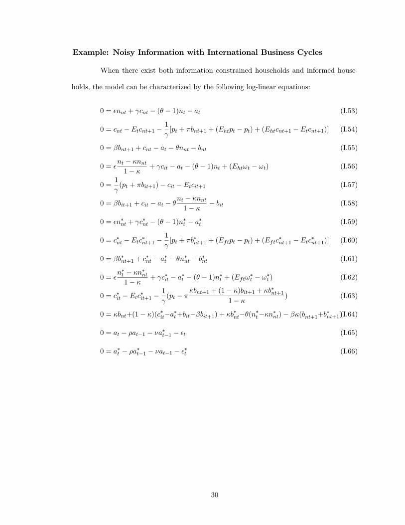
Figure 1 shows how the predicted correlation of �yt and �y�t changes in response
to changes in the relative precision of information ka=kx under two di¤erent asset market
assumptions. The left panel shows the complete market case based on (I.5) and the right
panel shows the incomplete market case based on (I.3). When the information is perfect
(ka=kx = 0), the output correlation is negative for the complete market. As ka=kx increases,
the correlation monotonically increases and becomes positive. In case of the incomplete
market, the output correlation is positive but is much smaller than what the data suggests.
Again, the correlation increases as ka=kx increases. For both cases, the model with a
su¢ ciently large noise matches the observed output correlation from the data (0.54 and
0.32).
An intuitive explanation on the role of restricted information in increasing output
correlation is as follows. The main reason why standard IRBC models generate negative or
near zero correlation of output is that the domestic and foreign �rms respond to technology
shocks in the opposite direction. For example, with a positive productivity shock in the
home country, domestic �rms increase their production, while foreign �rms decrease their
12

production. In contrast, if foreign �rms do not directly observe a positive shock at home
country, they do not reduce their production. Furthermore, as a result of excess supply
caused by uninformed foreign �rms, home �rms do not increase production as much as the
fully informed case. Combining the e¤ect of weaker responses with positively correlated
technologies across two countries can yield positive output correlation.
International Consumption Correlation (� = �� > 0)
We now focus on the bond-economy IRBC model when there are two types of
consumers. We show that introducing type 2 consumers in the economy will make the
international correlation of consumption lower compared to the benchmark model with
full information. To simplify the argument, we here maintain that the fraction of type 1
consumers is common across the countries. As in the previous subsection, we use the �rst
di¤erence �lter to investigate the international consumption correlation. Typically, the data
suggests that international consumption growth correlation is less than the international
output growth correlation. For example, Obstfeld and Rogo¤ (2000) use the annual Penn
World Table data over 1973 to 1992 and �nd that the average international correlation in
real GDP growth rates is 0.53, while the average consumption growth correlation is 0.40.
We also compute the consumption growth rate correlation based on the data from OECD
Quarterly National Accounts. If we use four countries for the Euro area, consumption
correlation is 0.46 compared to the outputs correlation of 0.54 during the period from
1989Q1 to 2009Q4. When we use 15 European countries to construct Euro aggregates,
the consumption correlation is 0.26, but the outputs correlation is 0.32. In either case,
consumption correlation is lower than the output correlation, which cannot be predicted by
the standard full information model.3
To solve the model with � = �� > 0, we need to combine an extended version of
3Pakko (2004) uses 10 country data from 1973:Q1 to 2002:Q4 and show that for all countries, the corre-lations of output growth rates is higher than that of consumption growth rates.
13

Sims�(2001) approach and the guess-veri�cation approach. We decompose heterogeneous
expectations into homogeneous expectation component and expectation error component.
We then solve the model by treating as if the latter is an exogenous shock in the �rst
step. In the second step, we use the method of undetermined coe¢ cients to assure the
endogenous expectation errors consistent with the solution from the �rst step (see technical
appendix for details). All the parameter values are the same as before except that we set
� = 0:6. The solutions are obtained for both (yt; y�t ) and (ct; c�t ) where ct = logCt � logC
and c�t = logC�t � logC�.
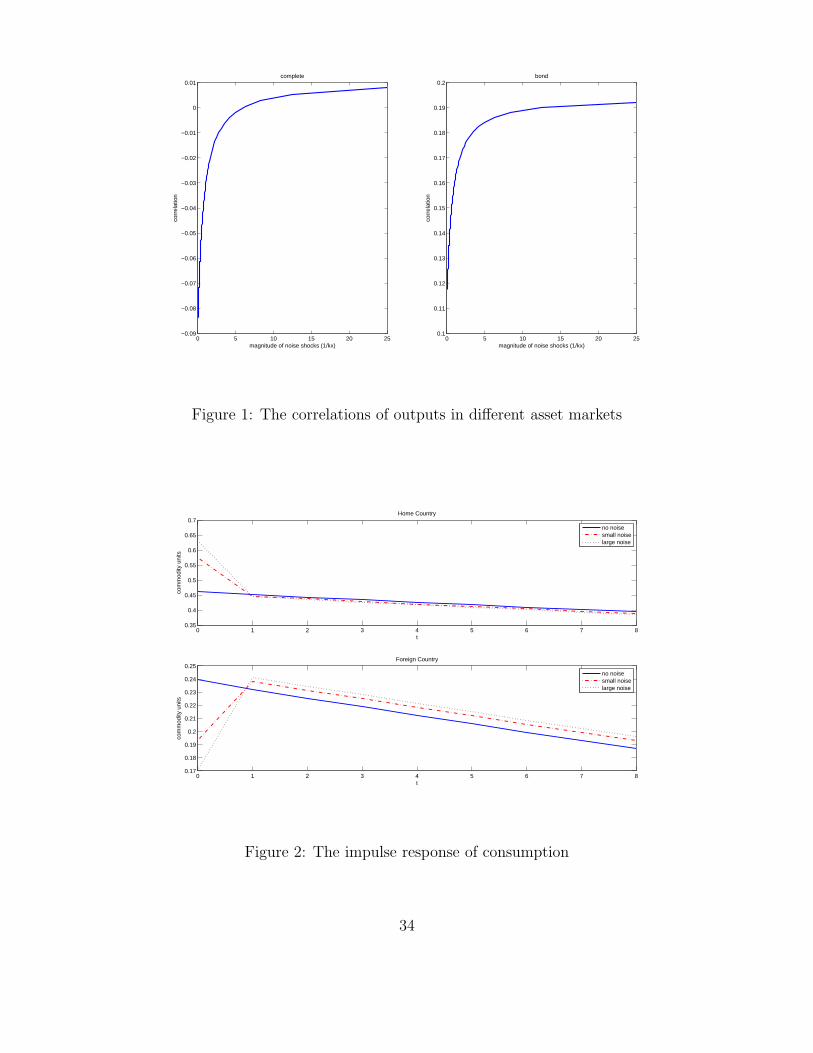
To understand the characteristics of the model, we compute the impulse response
of consumption to one standard positive deviation of domestic technology shocks with three
di¤erent choice of relative precision of information, ka=kx = 0, 1, and 25, which is shown
in Figure 24. Since the information is revealed at the end of each period, the e¤ects of
information precision become almost negligible after one period. In the perfect information
case (ka=kx = 0), households in the home country increase their consumptions as their
income increases. Households in the foreign country also increase consumption, since the
spillover e¤ects of the positive technology shocks make foreign households to borrow from
the home country. When the information noise becomes large (ka=kx = 1, and 25), foreign
households cannot predict the increase in income in the future and do not borrow as much
as they should from the international asset market. Therefore, even if foreign �rms produce
relatively more than the perfect information case, foreign households still decrease their
consumption. This asymmetric responses of ct and c�t is even more ampli�ed by taking the
�rst di¤erence �ct and �c�t . This makes consumption growth correlation decreasing with
respect to the magnitude of information noise.
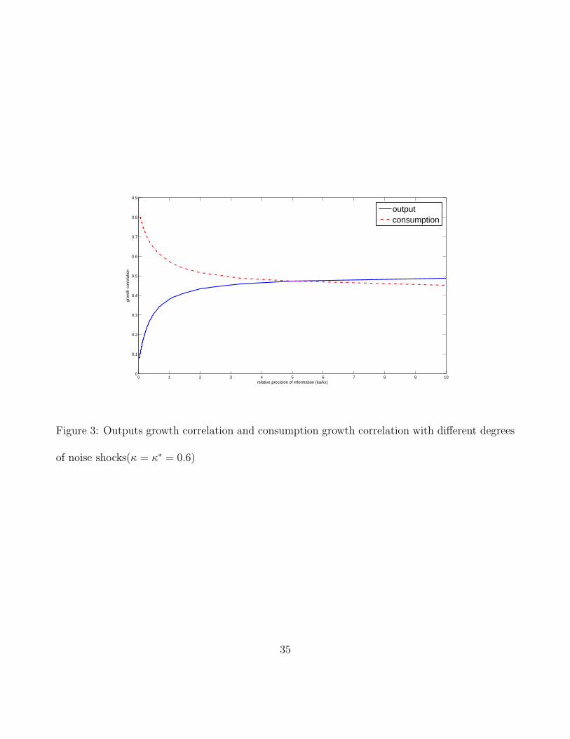
Figure 3 demonstrates the dynamics of consumptions growth correlation and out-
4Since both information-constrained and unconstrained consumers have rational expectations, as long as� is not extremely large the calibration of our exercise shows the response of interest rates to technologyshocks is not unrealistic.
14

puts growth correlation in response to di¤erent degrees of information frictions. As in the
case of � = �� = 0, we can see information noise increases outputs growth correlation, and
at the same time it reduces consumptions-growth correlation. When the relative precision
of information (ka=kx) reaches 5, the consumption growth correlation becomes less than
the output growth correlation which dramatically reduces the gap between the prediction
of the model and the data.
International Productivity-Hours Dynamics (� 6= ��)
In the recent global �nancial crisis of 2007-2009, employment and hours worked
declined both in the US and Euro area. Such a positive comovement is not predicted by the
standard IRBC models. Furthermore, since the labor declined more in the US than in Euro
area, observed labor productivity increased in the US which contrast to the Euro area where
near-zero or negative productivity growth was observed. This fact was �rst investigated by
Ohanian (2010). The empirical observation of near-zero (or negative) correlation between
productivity and hours worked has been viewed as a productivity-hours anomaly in the
macroeconomic literature since the standard real business cycle model predicts a positive
response of hours worked to positive technology shocks, provided an upward sloping labor
supply curve (see Galí, 1999; Christiano, Eichenbaum and Vigfusson, 2003).
Let us �rst show that given a certain range of parameter values, our model can
predict the positive comovement of labor input, which cannot be obtained in the full in-
formation model. In our data, the hours worked (growth) correlation between the US and
Euro area based on four European countries is positive at 0.20. Using the same solution
technique as before, we can obtain the solution for (nt; n�t ) where nt = logNt � logN and
n�t = logN�t � logN�. Figure 4 shows the predicted international correlation of hours
worked using the same set of parameter values as before. For the perfect information case
with ka=kx = 0, the correlation is negative. The correlation is not monotonically increasing
15

in ka=kx. However, it predicts the positive correlation when ka=kx lies between the values
of 0.1 and 0.5.
We also solve the model when the fraction of information constrained consumers
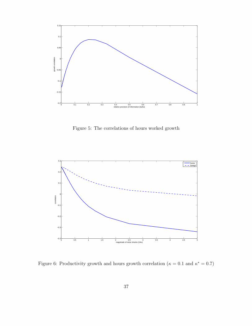
di¤ers across the country. Figure 5 shows the predicted correlation of hour worked growth,
�nt(�n�t ), and measured productivity growth, �yt ��nt(�y�t ��n�t ), when � = 0:1 and
�� = 0:7. It shows that when ka=kx increases, the model can predict negative productivity-
hours correlation in one region and positive productivity-hours correlation in the other
region (Figure 6), where the former represents the Euro area and the latter represents the
US.
The Model with Capital Accumulation
In this section, we extend our model, and show that our main results are consistent
for models with and without capital as an input in the production functions. The model
structure is the same as in section 2, and the only di¤erence is �rms�production functions
and households�budget-constraint equations. The production functions is
Yt = AtK1��t N �
t
for the home country and
Y �t = A�tK�1��t N��
t
for the foreign country, where Kt(K�t ) is the capital stock for the home (foreign) country. In
addition to investing in the �nancial capital market, households also invest in the physical
16

capital market. The households�budget constraint is
Ct + It +Bt+1 +�
2B2t+1 � rtKt +WtNt +RtBt
for the home country and
C�t + I�t +B
�t+1 +
�
2B�2t+1 � r�tKt +W
�t N
�t +RtB
�t
for the foreign country, if households can only trade real bonds across countries. If house-
holds can trade state-contingent bonds internationally, the households�budget constraint
becomes
Ct + C�t + It + I
�t = Yt + Y
�t ;
where It(I�t ) is the investment in the physical capital in the home (foreign) country and
rt(r�t ) is the interest rate in the capital renting market in the home (foreign) country. The
capital stock evolves according to
Kt+1 = (1� �)Kt + �(ItKt)Kt
for the home country and
K�t+1 = (1� �)K�
t + �(I�tK�t
)K�t
for the foreign country, where � is the capital depreciation rate and the function �(�) implies
an adjustment cost. The function 1=�0is Tobin�s q, which gives the number of units of
output which must be foregone to increase the capital stock in a particular location by one
unit.
The solution method is the same as the method used in section 3.2. We log-
linearize the �rst-order conditions of the model �rst, and then use an approach combining
an extended version of Sims� (2001) approach and the guess-veri�cation approach. To
calibrate the model, in addition to the parameters speci�ed before, we need specify two
17
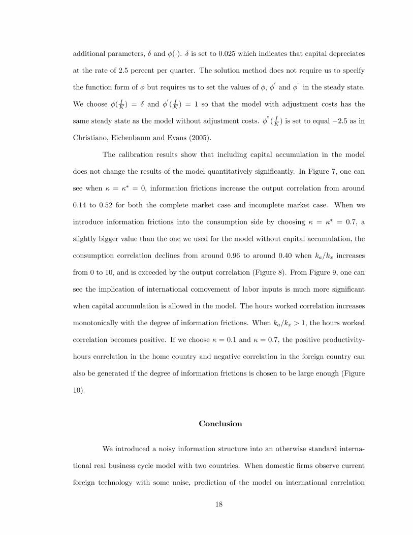
additional parameters, � and �(�). � is set to 0:025 which indicates that capital depreciates
at the rate of 2:5 percent per quarter. The solution method does not require us to specify
the function form of � but requires us to set the values of �, �0and �" in the steady state.
We choose �( IK ) = � and �0( IK ) = 1 so that the model with adjustment costs has the
same steady state as the model without adjustment costs. �"( IK ) is set to equal �2:5 as in
Christiano, Eichenbaum and Evans (2005).
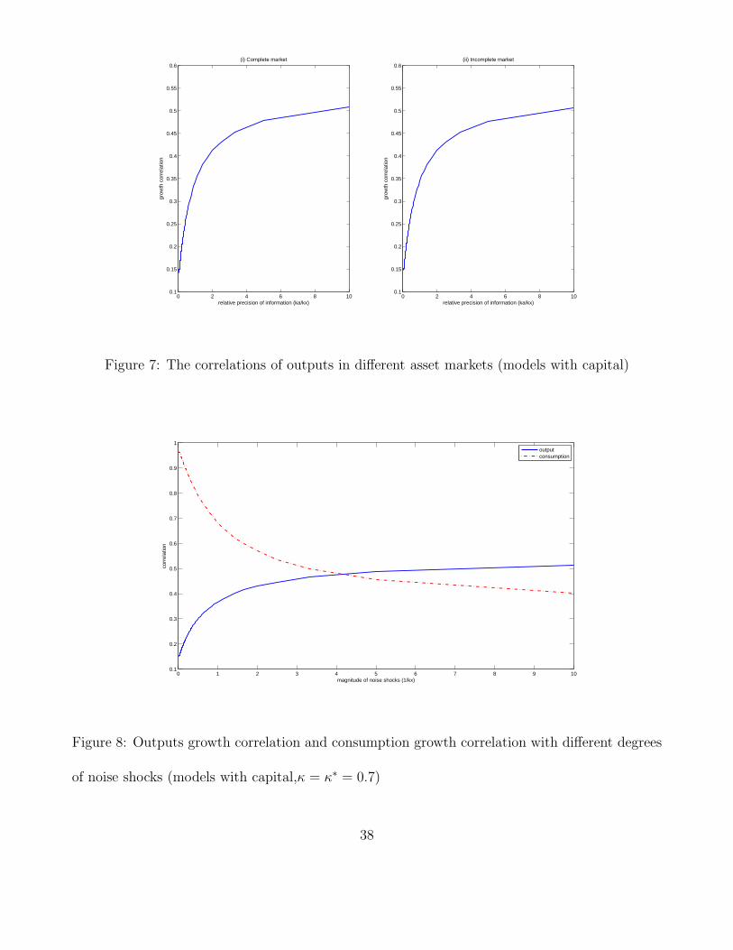
The calibration results show that including capital accumulation in the model
does not change the results of the model quantitatively signi�cantly. In Figure 7, one can
see when � = �� = 0, information frictions increase the output correlation from around
0:14 to 0:52 for both the complete market case and incomplete market case. When we
introduce information frictions into the consumption side by choosing � = �� = 0:7, a
slightly bigger value than the one we used for the model without capital accumulation, the
consumption correlation declines from around 0:96 to around 0:40 when ka=kx increases
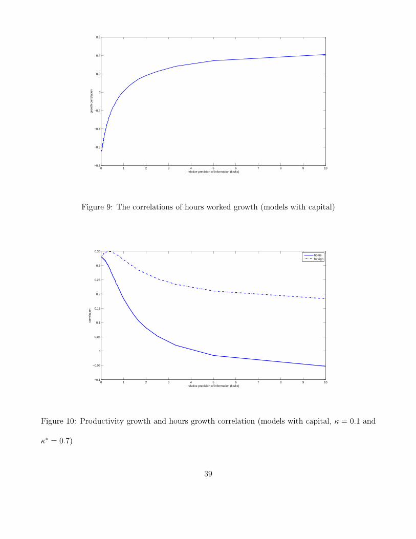
from 0 to 10, and is exceeded by the output correlation (Figure 8). From Figure 9, one can
see the implication of international comovement of labor inputs is much more signi�cant
when capital accumulation is allowed in the model. The hours worked correlation increases
monotonically with the degree of information frictions. When ka=kx > 1, the hours worked
correlation becomes positive. If we choose � = 0:1 and � = 0:7, the positive productivity-
hours correlation in the home country and negative correlation in the foreign country can
also be generated if the degree of information frictions is chosen to be large enough (Figure
10).
Conclusion
We introduced a noisy information structure into an otherwise standard interna-
tional real business cycle model with two countries. When domestic �rms observe current
foreign technology with some noise, prediction of the model on international correlation
18

turned out to be very di¤erent from that of a standard perfect information model. First, we
found that the imperfect information model can explain positive output correlation both in
complete and incomplete market models. Second, consumption correlation became smaller
than output correlation when the precision of the information becomes worse in the pres-
ence of information constrained households. Third, the model can explain the observation
of positive productivity-hours correlation in one country and negative correlation in the
other country.
There are several directions in which our model can be extended. First, we can
allow for information heterogeneity not only across the countries but also within a country.
When �rms in the same country face di¤erent signals about the foreign technology, the
lagged foreign technology will have a role of public information, in addition to its role as the
predictor of the current foreign technology. This may amplify the e¤ect of noisy information
and increase the predicted international output comovement. Second, we can introduce
nominal shocks into the model and consider the possibility of confusion between nominal
and real shocks. Third, we can investigate the role of the possible correlation of noise shocks
across countries for the output correlations. Finally, it would be another contribution to the
literature if one can estimate the parameters of variances of noise shocks and of proportions
of information-constrained households within a country5. These extensions are left for
future research.
5To the best of my knowledge, until now there is no estimation work on to what degree noise shockscan quantitatively explain business cycle �uctuations in a DSGE framework. Olivier J. Blanchard, GuidoLorenzoni, and Jean Paul L�Huillier (2012) use a structural vector autoregression (SVAR) and argue thatnoise shocks explain around half of business cycle �uctuations.
19
Appendix A
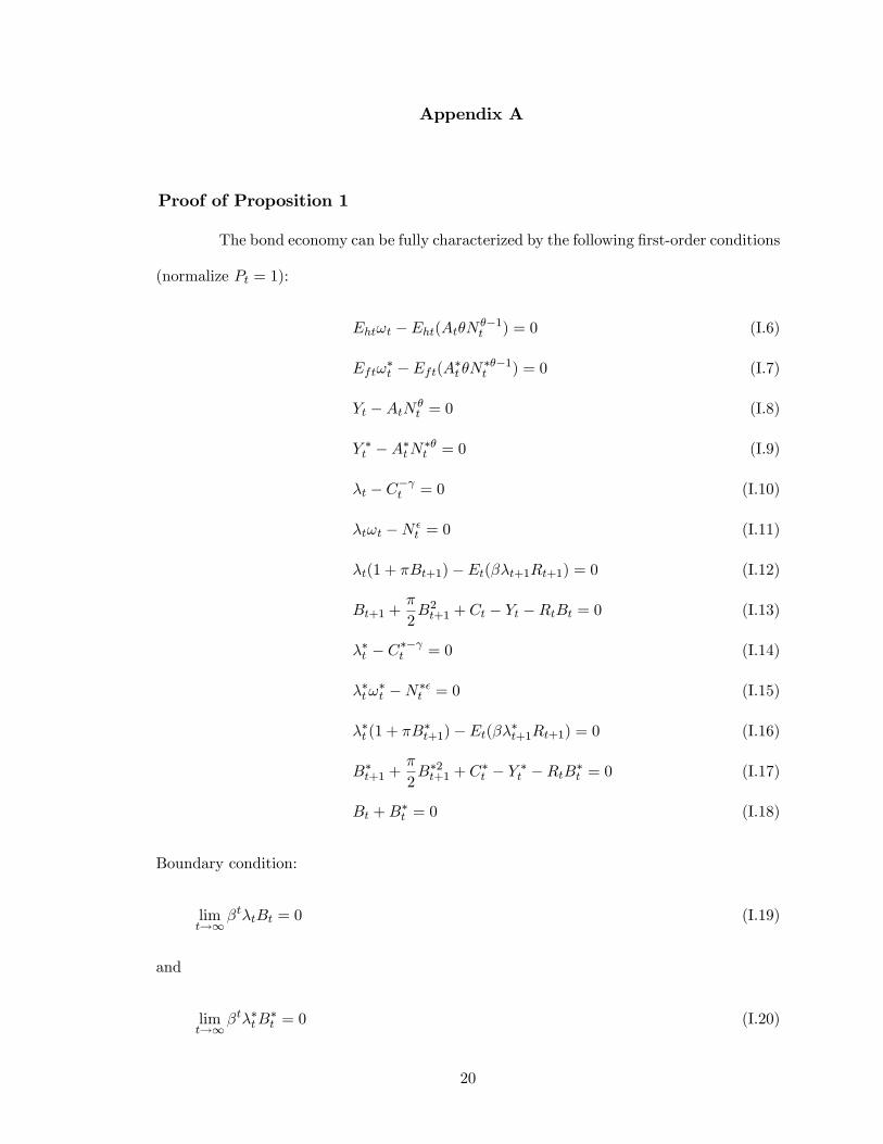
Proof of Proposition 1
The bond economy can be fully characterized by the following �rst-order conditions
(normalize Pt = 1):
Eht!t � Eht(At�N ��1t ) = 0 (I.6)
Eft!�t � Eft(A�t �N���1
t ) = 0 (I.7)
Yt �AtN �t = 0 (I.8)
Y �t �A�tN��t = 0 (I.9)
�t � C� t = 0 (I.10)
�t!t �N �t = 0 (I.11)
�t(1 + �Bt+1)� Et(��t+1Rt+1) = 0 (I.12)
Bt+1 +�
2B2t+1 + Ct � Yt �RtBt = 0 (I.13)
��t � C�� t = 0 (I.14)
��t!�t �N��
t = 0 (I.15)
��t (1 + �B�t+1)� Et(���t+1Rt+1) = 0 (I.16)
B�t+1 +�
2B�2t+1 + C
�t � Y �t �RtB�t = 0 (I.17)
Bt +B�t = 0 (I.18)
Boundary condition:
limt!1
�t�tBt = 0 (I.19)
and
limt!1
�t��tB�t = 0 (I.20)
20
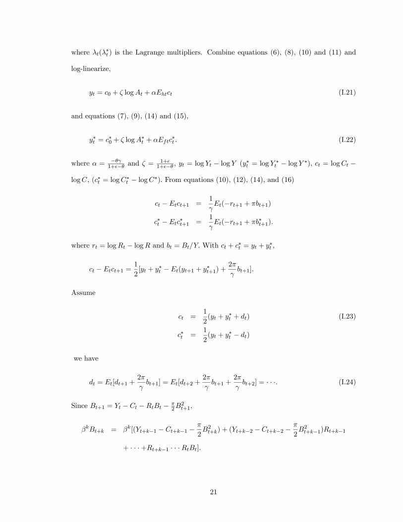
where �t(��t ) is the Lagrange multipliers. Combine equations (6), (8), (10) and (11) and
log-linearize,
yt = c0 + � logAt + �Ehtct (I.21)
and equations (7), (9), (14) and (15),
y�t = c�0 + � logA�t + �Eftc
�t : (I.22)
where � = �� 1+��� and � =
1+�1+��� , yt = log Yt � log Y (y�t = log Y
�t � log Y �), ct = logCt �
logC, (c�t = logC�t � logC�): From equations (10), (12), (14), and (16)
ct � Etct+1 =1
Et(�rt+1 + �bt+1)
c�t � Etc�t+1 =1
Et(�rt+1 + �b�t+1):
where rt = logRt � logR and bt = Bt=Y: With ct + c�t = yt + y�t ,
ct � Etct+1 =1
2[yt + y
�t � Et(yt+1 + y�t+1) +
2�
bt+1]:
Assume
ct =1
2(yt + y
�t + dt) (I.23)
c�t =1
2(yt + y
�t � dt)
we have
dt = Et[dt+1 +2�
bt+1] = Et[dt+2 +
2�
bt+1 +
2�
bt+2] = � � �: (I.24)
Since Bt+1 = Yt � Ct �RtBt � �2B
2t+1,
�kBt+k = �k[(Yt+k�1 � Ct+k�1 ��
2B2t+k) + (Yt+k�2 � Ct+k�2 �
�
2B2t+k�1)Rt+k�1
+ � � �+Rt+k�1 � � �RtBt]:
21

By using the boundary condition (19), limk!1Et�kBt+k = 0, in the steady state Y = C
and �R = 1, Yt � Ct � Y (yt � ct), and (24),
dt = (1� �)fEt[1Xk=0
�k(yt+k � y�t+k) +1Xk=0
�k+12�
(1� �)bt+1+k + 2bt]g: (I.25)
Use guess-veri�cation approach and assume
yt = m�1 logAt�1 +m��1 logA
�t�1 +m logAt +mxxt +mbbt (I.26)
y�t = m�1 logA�t�1 +m
��1 logAt�1 +m logA
�t +mxx
�t +mbb
�t (I.27)
and technology processes have the following vector-autoregressive form2664lnAtlnA�t
3775 =2664� �
� �
37752664lnAt�1lnA�t�1
3775+2664�t��t
3775 (I.28)
then
dt = (1� �)(m�1 �m��1)(logAt�1 � logA�t�1) +
1� �1� �(�� �) [�(m�1 �m�
�1) (I.29)
+m� �mx(�� �)](logAt � logA�t ) + (1� �)[mx(xt � x�t ) + (2mb +2�
(1� �))
�Et1Xk=0
�kbt+k + (2�2�
(1� �))bt]: (I.30)
Plug (25) into (24),
Et[
1Xk=0
�k(yt+k � y�t+k) + (2mb +2�
(1� �))1Xk=0
�kbt+k + (2�2�
(1� �))bt](I.31)
= Et[
1Xk=0
�k(yt+1+k � y�t+1+k) + (2mb +2�
(1� �))1Xk=0
�kbt+1+k + 2bt+1]:
22
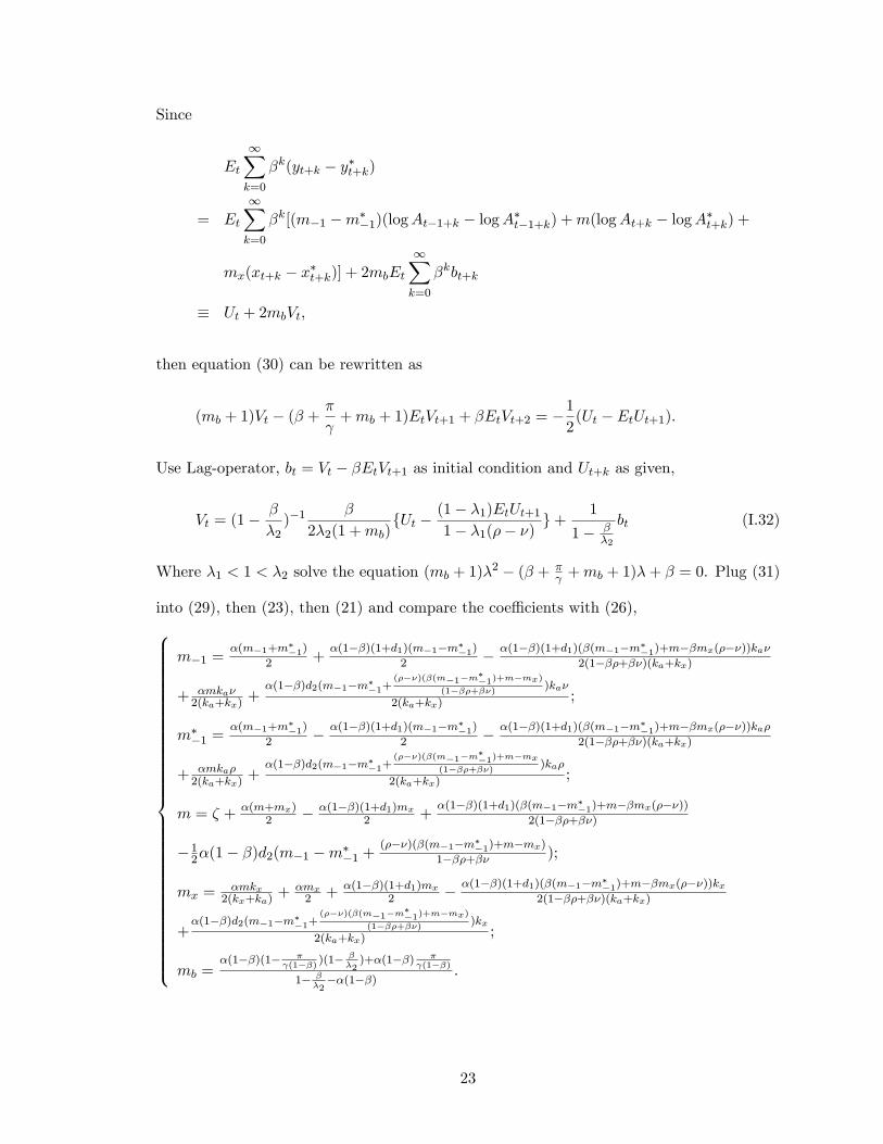
Since
Et
1Xk=0
�k(yt+k � y�t+k)
= Et
1Xk=0
�k[(m�1 �m��1)(logAt�1+k � logA�t�1+k) +m(logAt+k � logA�t+k) +
mx(xt+k � x�t+k)] + 2mbEt
1Xk=0
�kbt+k
� Ut + 2mbVt;
then equation (30) can be rewritten as
(mb + 1)Vt � (� +�
+mb + 1)EtVt+1 + �EtVt+2 = �
1
2(Ut � EtUt+1):
Use Lag-operator, bt = Vt � �EtVt+1 as initial condition and Ut+k as given,
Vt = (1��
�2)�1
�
2�2(1 +mb)fUt �
(1� �1)EtUt+11� �1(�� �)
g+ 1
1� ��2
bt (I.32)
Where �1 < 1 < �2 solve the equation (mb + 1)�2 � (� + �
+mb + 1)�+ � = 0. Plug (31)
into (29), then (23), then (21) and compare the coe¢ cients with (26),8>>>>>>>>>>>>>>>>>>>>>>>>>>>>>>><>>>>>>>>>>>>>>>>>>>>>>>>>>>>>>>:
m�1 =�(m�1+m�
�1)2 +
�(1��)(1+d1)(m�1�m��1)
2 � �(1��)(1+d1)(�(m�1�m��1)+m��mx(���))ka�
2(1���+��)(ka+kx)
+ �mka�2(ka+kx)
+�(1��)d2(m�1�m�
�1+(���)(�(m�1�m
��1)+m�mx)
(1���+��) )ka�
2(ka+kx);
m��1 =
�(m�1+m��1)
2 � �(1��)(1+d1)(m�1�m��1)
2 � �(1��)(1+d1)(�(m�1�m��1)+m��mx(���))ka�
2(1���+��)(ka+kx)
+ �mka�2(ka+kx)
+�(1��)d2(m�1�m�
�1+(���)(�(m�1�m
��1)+m�mx
(1���+��) )ka�
2(ka+kx);
m = � + �(m+mx)2 � �(1��)(1+d1)mx
2 +�(1��)(1+d1)(�(m�1�m�
�1)+m��mx(���))2(1���+��)
�12�(1� �)d2(m�1 �m�
�1 +(���)(�(m�1�m�
�1)+m�mx)
1���+�� );
mx =�mkx
2(kx+ka)+ �mx
2 + �(1��)(1+d1)mx
2 � �(1��)(1+d1)(�(m�1�m��1)+m��mx(���))kx
2(1���+��)(ka+kx)
+�(1��)d2(m�1�m�
�1+(���)(�(m�1�m
��1)+m�mx)
(1���+��) )kx
2(ka+kx);
mb =�(1��)(1� �
(1��) )(1���2)+�(1��) �
(1��)
1� ��2��(1��)
:
23
where � = �� 1+��� , � =
1+�1+��� , d1 = (mb+
� (1��))(1�
��2)�1 �
(�2(1+mb), d2 = (mb+
� (1��))(1�
��2)�1 �(1��1)
(�2(1+mb)[1��1(���)] . There are �ve undetermined variables and �ve equations, so we
solve the coe¢ cients (m�1;m��1;m;mx;m
�x). We can easily verify that mb is invariant to
ka=kx.
For part (ii), when ka=kx ! 0, the above equations become8>>>>>>>>>>>>>>>>>>>>>>><>>>>>>>>>>>>>>>>>>>>>>>:
m�1 =�(m�1+m�
�1)2 +
�(1��)(1+d1)(m�1�m��1)
2 ;
m��1 =
�(m�1+m��1)
2 � �(1��)(1+d1)(m�1�m��1)
2 ;
m = � + �(m+mx)2 � �(1��)(1+d1)mx
2 +�(1��)(1+d1)(�(m�1�m�
�1)+m��mx(���))2(1���+��)
�12�(1� �)d2(m�1 �m�
�1 +(���)(�(m�1�m�
�1)+m�mx)
1���+�� );
mx =�(m+mx)
2 + �(1��)(1+d1)mx
2 � �(1��)(1+d1)(�(m�1�m��1)+m��mx(���))
2(1���+��)
+�(1��)d2(m�1�m�
�1+(���)(�(m�1�m
��1)+m�mx)
(1���+��) )
2 ;
mb =�(1��)(1� �
(1��) )(1���2)+�(1��) �
(1��)
1� ��2��(1��)
:
so, 8>>>>>>>>>>><>>>>>>>>>>>:
m�1 = m��1 = 0;
m = �1�� �
�[(1���+��)�(1��)(1+d1)+(1��)d2(���)]�2(1��)[(1���+��)��(1��)(1+d1)+�(1��)d2(���)] ;
mx =�[(1���+��)�(1��)(1+d1)+(1��)d2(���)]�
2(1��)[(1���+��)��(1��)(1+d1)+�(1��)d2(���)] ;
mb =�(1��)(1� �
(1��) )(1���2)+�(1��) �
(1��)
1� ��2��(1��)
:
Then, let us proof the case under the condition � ! 0, m > 0 and mx < 0. Let us prove
�1 < mb < 0 as a preparation for later proofs. Since 0 < �1 < 1 < �2, 0 < � < 1;and
� < 0; ��2 < 1; if � ! 0, we have mb < 0 and,
mb + 1 =(1� �
�2)(1� �(1� �)) + ���
�2
1� ��2� �(1� �)
> 0:
24
Therefore, we have �1 < mb < 0: Next,
d1 = (mb +�
(1� �))(1��
�2)�1
�
�2(1 +mb)
=�(1� �)� ��
+�
(1��)
1� ��2� �(1� �)
�
�2(1 +mb)=
��(1��)�2
� ��� �2
+ �� �2(1��)
���(1��)�2
+ ��� �2
+ 1� ��2
< 0:
Similarly, we can also have d2 < 0:
�d2(�� �) < �d2 = �d11� �1
1� �1(�� �)< �d1;
so we have �d1 + d2(�� �) > 0: Therefore, mx�s numerator:
�[(1� ��+ ��)� (1� �)(1 + d1) + (1� �)d2(�� �)]�
= �f� � ��+ �� + (1� �)[�d1 + d2(�� �)]g < 0:
Furthermore,
d1 + 1 =1� �
�2+ ��
�2(1��)
���(1��)�2
+ ��� �2
+ 1� ��2
> 0:
mx�s denominator
2(1� �)[(1� ��+ ��)� �(1� �)(1 + d1) + �(1� �)d2(�� �)] > 0:
Overall,
mx =�[(1� ��+ ��)� (1� �)(1 + d1) + (1� �)d2(�� �)]�
2(1� �)[(1� ��+ ��)� �(1� �)(1 + d1) + �(1� �)d2(�� �)]< 0:
Note that m+mx =�
1�� > 0; so m > 0.
25

Proof of Proposition 2
The complete-market economy can be fully characterized by the following �rst-
order conditions:
Eht!t � Eht(At�N ��1t ) = 0 (I.33)
Eft!�t � Eft(PtA�t �N���1
t ) = 0 (I.34)
Yt �AtN �t = 0 (I.35)
Y �t �A�tN��t = 0 (I.36)
C� t � C�� t = 0 (I.37)
N �t � C
� t !t = 0 (I.38)
N��t � C�� t !�t = 0 (I.39)
Ct + C�t �AtN �
t �A�tN��t = 0: (I.40)
From equations (32), (34) and (37)
yt = c0 + � logAt + �Ehtct (I.41)
and equations (33), (35) and (38)
y�t = c�0 + � logA�t + �Eftc
�t (I.42)
where the constant terms c0 = c�0 =�
1+"�� , � � ��
1+��� and � �1+�1+��� . Since Ct = C�t , we
have:
ct = c�t =1
2[yt + y
�t ]: (I.43)
Use guess-veri�cation approach and assume
yt = m�1 logAt�1 +m��1 logA
�t�1 +m logAt +mxxt
y�t = m�1 logA�t�1 +m
��1 logAt�1 +m logA
�t +mxx
�t
26
and plug the two above equations into equation (42), and then (40), we have
m0 +m�1 logAt�1 +m��1 logA
�t�1 +m logAt +mxxt
= c0 + � logAt + �fm0 +m�1 +m�
�12
logAt�1 +m�1 +m�
�12
logA�t�1
+m[ka(� logA
�t�1 + � logAt�1) + kxxt]
2(ka + kx)+m
2logAt +
mx
2xt +
mx
2logAtg:
Compare the coe¢ cients in the above equation,
m�1 = �m�1 +m�
�12
+m��ka2(ka + kx)
(I.44)
m��1 = �
m�1 +m��1
2+
m��ka2(ka + kx)
(I.45)
m = � + �m+mx
2(I.46)
mx = �[mx
2+
mkx2(ka + kx)
] (I.47)
Solve equations (42) to (46), and ignore the constant term, we have,
8>>>>>>>>>><>>>>>>>>>>:
m =(1��
2)�(ka+kx)
(1��2)2ka+(1��)kx ;
mx =�2�kx
(1��2)2ka+(1��)kx ;
m�1 =[�2�+(1��
2)�](1��
2)��
2(1��)[(1��2)2ka+(1��)kx]ka;
m��1 =
[(1��2)�+�
2�](1��
2)��
2(1��)[(1��2)2ka+(1��)kx]ka:
:
For part (ii), when ka=kx ! 0, it is straightforward to have that the coe¢ cients
(m�1;m��1;m;mx) approaches (0; 0;
1��2
1�� �;�2
1���).
Appendix B
This appendix brie�y describes a method to solve a system of linear expectational
di¤erence equations with heterogeneous information. At �rst, we divide heterogeneous
expectational operators into two components, the full information part and the expectation
errors part. The expectation errors part is then treated as shocks to the model, and then we
solve the system of linear expectational di¤erence equations as the case with homogeneous
information by Sims�s (2001) method in the �rst step. In the second step, we use the method
27
of undetermined coe¢ cients to assure the endogenous expectation errors consistent with the
solution from the �rst step. Let y(t) be a vector (k � 1) which we are interested in. Then
a typical system of linear rational expectational di¤erence equations with heterogeneous
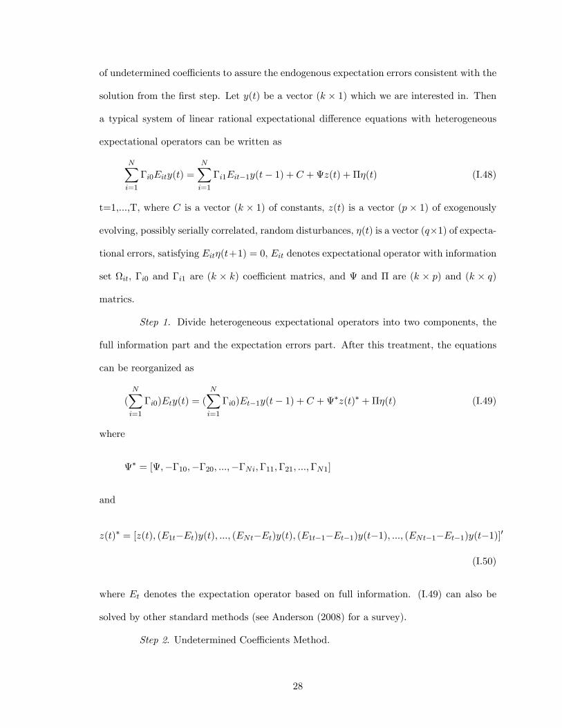
expectational operators can be written as
NXi=1
�i0Eity(t) =NXi=1
�i1Eit�1y(t� 1) + C +z(t) + ��(t) (I.48)
t=1,...,T, where C is a vector (k � 1) of constants, z(t) is a vector (p � 1) of exogenously
evolving, possibly serially correlated, random disturbances, �(t) is a vector (q�1) of expecta-
tional errors, satisfying Eit�(t+1) = 0, Eit denotes expectational operator with information
set it, �i0 and �i1 are (k � k) coe¢ cient matrics, and and � are (k � p) and (k � q)
matrics.
Step 1. Divide heterogeneous expectational operators into two components, the
full information part and the expectation errors part. After this treatment, the equations
can be reorganized as
(NXi=1
�i0)Ety(t) = (NXi=1
�i0)Et�1y(t� 1) + C +�z(t)� +��(t) (I.49)
where
� = [;��10;��20; :::;��Ni;�11;�21; :::;�N1]
and
z(t)� = [z(t); (E1t�Et)y(t); :::; (ENt�Et)y(t); (E1t�1�Et�1)y(t�1); :::; (ENt�1�Et�1)y(t�1)]0
(I.50)
where Et denotes the expectation operator based on full information. (I.49) can also be
solved by other standard methods (see Anderson (2008) for a survey).
Step 2. Undetermined Coe¢ cients Method.
28

By using Sims�s (2001) method, the solution of (I.49) can be characterized as
y(t) = �1y(t� 1) + �c +�0z�(t) + �y1Xs=1
�s�1f QzEtz�(t+ s) (I.51)
where the coe¢ cients are de�ned in equations (44) and (45) by Sims (2001). To use
undetermined coe¢ cients method, �rst, we list all the exogenous innovations by �(t) �
(�1t; �2t; :::; �lt) which might a¤ect the solution of y(t). The state variables �its could be
technology innovations, information signals, or other type of shocks. We then assume
z�(t) = ��0(t) (I.52)
where � is the ((p + kN) � l) undetermined coe¢ cients matrix. Remember that the top
entry of z�t is zt, so the �rst p row of � should also be known at this point and in total we
have kN � l unknown coe¢ cients. Plug equation (I.52) into (I.51), and we can have y(t).
Then plug the y(t) into the de�nition of z�(t) (I.50), and �nally match the coe¢ cients in
equation (I.52). We will have exactly the same number of linear equations as of unknown
variables, so we can exactly identify the unknown matrix �. Because it is a linear equations,
the solution procedure will not take too much time by using regular matrix-based software.
29
Example: Noisy Information with International Business Cycles
When there exist both information constrained households and informed house-
holds, the model can be characterized by the following log-linear equations:
0 = �nnt + cnt � (� � 1)nt � at (I.53)
0 = cnt � Etcnt+1 �1
[pt + �bnt+1 + (Ehtpt � pt) + (Ehtcnt+1 � Etcnt+1)] (I.54)
0 = �bnt+1 + cnt � at � �nnt � bnt (I.55)
0 = �nt � �nnt1� � + cit � at � (� � 1)nt + (Eht!t � !t) (I.56)
0 =1
(pt + �bit+1)� cit � Etcit+1 (I.57)
0 = �bit+1 + cit � at � �nt � �nnt1� � � bit (I.58)
0 = �n�nt + c�nt � (� � 1)n�t � a�t (I.59)
0 = c�nt � Etc�nt+1 �1
[pt + �b
�nt+1 + (Eftpt � pt) + (Eftc�nt+1 � Etc�nt+1)] (I.60)
0 = �b�nt+1 + c�nt � a�t � �n�nt � b�nt (I.61)
0 = �n�t � �n�nt1� � + c�it � a�t � (� � 1)n�t + (Eft!�t � !�t ) (I.62)
0 = c�it � Etc�it+1 �1
(pt � �
�bnt+1 + (1� �)bit+1 + �b�nt+11� � ) (I.63)
0 = �bnt+(1� �)(c�it�a�t+bit��bit+1) + �b
�nt��(n
�t��n
�nt)� ��(bnt+1+b
�nt+1)(I.64)
0 = at � �at�1 � �a�t�1 � �t (I.65)
0 = a�t � �a�t�1 � �at�1 � ��t (I.66)
30

So
z�t =
26666666666666666666666666664
�t
��t
Ehtpt � pt
Eht!t � !t
Eftpt � pt
Eft!�t � !�t
Ehtcnt+1 � Etcnt+1
Eftc�nt+1 � Etc�nt+1
37777777777777777777777777775At �rst, we solve the models and get the equation (I.51), then assume
z�t =
���������������������������������
1 0 0 0
0 1 0 0
p1 p2 p3 p4
!1 !2 !3 !4
p�1 p�2 p�3 p�4
!�1 !�2 !�3 !�4
c1 c2 c3 c4
c�1 c�2 c�3 c�4
���������������������������������
�
266666666664
�t
��t
vt
v�t
377777777775
Use the algorithm discussed above, we solve the models.
Appendix C
We choose US versus the Euro as the two countries in our model. To construct
the Euro aggregator we choose the following four countries: Austria, France, Germany,
31

and Spain. The following �les are used for average weekly hours worked per worker in
manufacturing.
Austria: we collect Monthly hours of work per month in manufacturing data from
LABORSTA. Then we use arithmetic mean of every three months to calculate the quarterly
hours of work per month in manufacturing. The data cover wage earners from 1989M1 to
1995M12. After that the data cover employees6.
France: we collect Quarterly hours of work per week in manufacturing data from
LABORSTA. The data cover wage earners from 1989Q1 to 1992Q4. From 1993Q1 to
2009Q4, the main coverage is for employees.
Germany: before 2005, LABORSTA has two di¤erent sequences for Germany:
Western Germany and Eastern Germany, but Western Germany covers both of two parts
after 1990Q1. After 2005, there is only one Germany sequence. We choose the sequence of
Western Germany to supplement the Germany sequence to have a complete data series of
Germany. The data cover wage earners.
Spain: we collect quarterly hours of work per week data from LABORSTA. The
data cover wage earners. There are two missing observations and we use the average of the
two closest observations to replace them.
All the raw data are not seasonally adjusted. We use X-12-ARIMA to seasonally
adjust them.
From above, we have the data of quarterly average hours of work per week or per
month in manufacturing. We collect the data of average annual hours actually worked per
worker in all sectors from OECD Main Economic Indicator. Then we use the quarterly
average hours of worker per week or per month in manufacturing as proportions to divide
the annual hours worked per worker in all sector to construct the quarterly hours of work
in all sectors data.6Because we use the series of quarterly hours of work as proportions to divide the series of annual hours
of work, so we conjecture the change of coverage only has a minor e¤ect.
32

Employment: we use quarterly average employment data from OECD Main Eco-
nomic Indicator. The data is seasonally adjusted.
Output and Consumption: the data for quarterly GDP and quarterly consumption
are from OECD Quarterly National Accounts.
The series for US quarterly average hours of work per week and employment are
from BLS. The series for US consumption and GDP are from OECD Quarterly National
Accounts.
33
0 5 10 15 20 25−0.09
−0.08
−0.07
−0.06
−0.05
−0.04
−0.03
−0.02
−0.01
0
0.01complete
magnitude of noise shocks (1/kx)
corr
elat
ion
0 5 10 15 20 250.1
0.11
0.12
0.13
0.14
0.15
0.16
0.17
0.18
0.19
0.2bond
magnitude of noise shocks (1/kx)
corr
elat
ion
Figure 1: The correlations of outputs in different asset markets
0 1 2 3 4 5 6 7 80.35
0.4
0.45
0.5
0.55
0.6
0.65
0.7
t
com
mod
ity u
nits
Home Country
no noisesmall noiselarge noise
0 1 2 3 4 5 6 7 80.17
0.18
0.19
0.2
0.21
0.22
0.23
0.24
0.25
t
com
mod
ity u
nits
Foreign Country
no noisesmall noiselarge noise
Figure 2: The impulse response of consumption
34
0 1 2 3 4 5 6 7 8 9 100
0.1
0.2
0.3
0.4
0.5
0.6
0.7
0.8
0.9
relative precision of information (ka/kx)
grow
th c
orre
latio
n
outputconsumption
Figure 3: Outputs growth correlation and consumption growth correlation with different degrees
of noise shocks(κ = κ∗ = 0.6)
35
GDP Labor Force (age 16-64)
Hours Per Labor Force Employment
Productivity (hours based) Productivity (Employment based)
0.85
0.9
0.95
1
1.05
us
euro0.9
0.920.940.960.98
11.02
2004
.120
04.4
2005
.320
06.2
2007
.120
07.4
2008
.320
09.2
us
euro
0.880.9
0.920.940.960.98
11.02
2004.1
2004.4
2005.3
2006.2
2007.1
2007.4
2008.3
2009.2
us
euro0.860.88
0.90.920.940.960.98
11.02
2004.1
2004.4
2005.3
2006.2
2007.1
2007.4
2008.3
2009.2
us
euro
1.11.041.06
Solow Residual (hours) Solow Residual (employment)
Figure 4: Labor Productivity and Hours Worked during the Recent Financial Crisis
36
0.9
0.95
1
1.05
1.1
2004.1
2004.4
2005.3
2006.2
2007.1
2007.4
2008.3
2009.2
us
euro0.9
0.920.940.960.98
11.021.041.06
2004.1
2004.4
2005.3
2006.2
2007.1
2007.4
2008.3
2009.2
us
euro
0.9
0.95
1
1.05
1.1
2004.1
2004.4
2005.3
2006.2
2007.1
2007.4
2008.3
2009.2
us
euro0.9
0.920.940.960.98
11.021.041.06
2004.1
2004.4
2005.3
2006.2
2007.1
2007.4
2008.3
2009.2
us
euro
0 0.1 0.2 0.3 0.4 0.5 0.6 0.7 0.8 0.9 1−0.2
−0.15
−0.1
−0.05
0
0.05
0.1
0.15
relative precision of information (ka/kx)
grow
th c
orre
latio
n
Figure 5: The correlations of hours worked growth
0 0.5 1 1.5 2 2.5 3 3.5 4 4.5 5−0.4
−0.3
−0.2
−0.1
0
0.1
0.2
0.3
magnitude of noise shocks (1/kx)
corr
elat
ion
homeforeign
Figure 6: Productivity growth and hours growth correlation (κ = 0.1 and κ∗ = 0.7)
37
0 2 4 6 8 100.1
0.15
0.2
0.25
0.3
0.35
0.4
0.45
0.5
0.55
0.6(i) Complete market
relative precision of information (ka/kx)
grow
th c
orre
latio
n
0 2 4 6 8 100.1
0.15
0.2
0.25
0.3
0.35
0.4
0.45
0.5
0.55
0.6(ii) Incomplete market
relative precision of information (ka/kx)
grow
th c
orre
latio
n
Figure 7: The correlations of outputs in different asset markets (models with capital)
0 1 2 3 4 5 6 7 8 9 100.1
0.2
0.3
0.4
0.5
0.6
0.7
0.8
0.9
1
magnitude of noise shocks (1/kx)
corr
elat
ion
outputconsumption
Figure 8: Outputs growth correlation and consumption growth correlation with different degrees
of noise shocks (models with capital,κ = κ∗ = 0.7)
38
0 1 2 3 4 5 6 7 8 9 10−0.8
−0.6
−0.4
−0.2
0
0.2
0.4
0.6
relative precision of information (ka/kx)
grow
th c
orre
latio
n
Figure 9: The correlations of hours worked growth (models with capital)
0 1 2 3 4 5 6 7 8 9 10−0.1
−0.05
0
0.05
0.1
0.15
0.2
0.25
0.3
0.35
relative precision of information (ka/kx)
corr
elat
ion
homeforeign
Figure 10: Productivity growth and hours growth correlation (models with capital, κ = 0.1 and
κ∗ = 0.7)
39
CHAPTER II
FINITE SAMPLE PERFORMANCE OF PRINCIPAL COMPONENTS ESTIMATORSFOR DYNAMIC FACTOR MODELS: ASYMPTOTIC AND BOOTSTRAP
APPROXIMATIONS
Introduction
The estimation of dynamic factor models has become popular in macroeconomic
analysis since in�uential works by Sargent and Sims (1977), Geweke (1977) and Stock and
Watson (1989). Later studies by Stock and Watson (1998, 2002), Bai and Ng (2002) and
Bai (2003) emphasize the consistency of the principal components estimator of unobservable
common factors under the asymptotic framework with a large number of cross-sectional
observations. This paper investigates the �nite sample properties of two-step persistence
estimators in dynamic factor models when unobservable common factors are estimated by
the principal components method in the �rst step. The �rst-step estimation is followed
by the estimation of autoregressive models of common factors in the second step. Using
analytical results and simulation experiments, we evaluate the e¤ect of the number of the
series (N) relative to the time series observations (T ) on the performance of the two-
step estimator of a persistence parameter. Furthermore, we propose a simple bootstrap
procedure that works well when N is relatively small.
In this paper, we focus on the persistence parameter of the common factor be-
cause of its empirical relevance in macroeconomic analysis. In modern macroeconomics
literature, dynamic stochastic general equilibrium (DSGE) models predict that a small set
of driving forces is responsible for covariation in macroeconomic variables. Theoretically,
the persistence of the common factor often plays a key role on implications of these models.
For example, in the real business cycle model, there is a well-known trade-o¤ between the
persistence of the technology shock and the performance of the model. When the shock
becomes more persistent, the performance improves along some dimensions but deteriorates
40

along other dimensions (King et al., 1988, Hansen, 1997, Ireland, 2001). In DSGE models
with a monetary sector, the optimal monetary policy largely depends on the persistence
of real shocks in the economy (Woodford, 1999). In open economy models, the welfare
gain from the introduction of international risk-sharing becomes larger when the technol-
ogy shock becomes more persistent (Baxter and Crucini, 1995). Since these common shocks
are not directly observable, a dynamic factor model o¤ers a simple robust statistical frame-
work for measuring the persistence of the common components that cause macroeconomic
�uctuations.1
Dynamic factor models have also been used to construct a business cycle index
(e.g., Stock and Watson, 1989, Kim and Nelson, 1993) and to extract a measure of underly-
ing, or core, in�ation (e.g., Bryan and Cecchetti, 1993). In such applications, the persistence
of a single factor can often be of main interest. For example, Clark (2006) examines the
possibility of a structural shift in the persistence of a single common factor estimated using
the �rst principal component of disaggregate in�ation series. In this paper, we consider
only the case in which a single common factor is generated from a univariate autoregressive
(AR) model of order one. This speci�cation keeps our problem simple since the persistence
measure corresponds to the AR coe¢ cient. However, in principle, the main idea of our
approach can be applicable to AR models of higher order.2
The principal components estimation of the unobserved common factors is com-
putationally simple and feasible with a large number of cross-sectional observations N .
The method also allows for an approximate factor structure with possible cross-sectional
correlations of idiosyncratic errors.3 The large N asymptotic results obtained by Connor
and Korajczyk (1986) and Bai (2003) implypN -consistency of the principal components
estimators of common factors up to a scaling constant. Therefore, if N is su¢ ciently large,
we can treat the estimated common factor as if we directly observe the true common factor
when conducting inference. However, since this argument is based on the asymptotic the-
1Recently, Boivin and Giannoni (2006) proposed estimating a dynamic factor model in which they imposethe full structure of the DSGE model on the transition equation of the latent factors.
2In the case of AR models of higher order, however, there are several measures of persistence, includingthe sum of AR coe¢ cients, largest characteristic root and �rst-order autocorrelation.
3The principle components estimator of the common factor with large N can also be used to estimatenonlinear models (Connor, Korajczyk and Linton, 2006, Diebold, 1998, Shintani, 2005, 2008) or to test thehypothesis of a unit root (Bai and Ng, 2004, and Moon and Perron, 2004).
41
ory, an approximation may not work when N is small relative to the time series observation
T that is typically available in practice. Consistent with our theoretical prediction, the
results from our Monte Carlo experiment using positively autocorrelated factors suggest
the downward bias in the AR coe¢ cient estimator and signi�cant under-coverage of the
naive con�dence interval when N is small. The simulation results also suggest that a simple
bootstrap procedure works well in correcting the bias and improves the performance of the
con�dence interval.
The bootstrap part of our analysis is closely related to recent studies by Gonçalves
and Perron (2012) and Yamamoto (2012). Both papers also employ bootstrap procedures
for the purpose of improving the �nite sample performance of estimators of dynamic factor
models. Gonçalves and Perron (2012) employ a bootstrap procedure in factor-augmented
forecasting regression models with multiple factors. The factor-augmented forecasting re-
gression models are very useful in utilizing information from many predictors without in-
cluding too many regressors. This aspect is emphasized in Stock and Watson (1998, 2002),
Marcellino, Stock and Watson (2003) and Bai and Ng (2006), among others. Gonçalves
and Perron (2012) provide the �rst order asymptotic validity of their bootstrap procedure
for factor-augmented forecasting regression models, but not in the context of estimation
of the persistence parameter of the common factor. It should also be noted that, unlike
their factor-augmented forecasting regression models with multiple factors, the bootstrap
procedure for our univariate AR model of the common factor is not subject to scaling and
rotation issues.4 Yamamoto (2012) examines the performance of the bootstrap procedure
applied to the factor-augmented vector autoregressive (FAVAR) models of Bernanke, Boivin
and Eliasz (2005). While his multiple factor structure is more general than our single fac-
tor structure, his main focus is the identi�cation of structural parameters in the FAVAR
analysis using various identifying assumptions. In contrast, we are more interested in the
role of parameters in the model in explaining the deviation from the large N asymptotics
when N is small.4To be more speci�c, under our normalizing assumption, the factor is estimated up to sign but the au-
toregressive coe¢ cient can be identifed as the sign cancels out from both side of the autoregressive equation.
42
There are several simulation results available in the literature on the principal
components estimator of dynamic factor models. Stock and Watson (1998) report the �nite
sample simulation results on the magnitude of the �rst-step estimation error of the common
factor as well as the performance of an out-of-sample forecast based on the estimated factor
relative to that of an infeasible forecast with a true factor. Boivin and Ng (2006) report
similar performance measures in investigating the marginal e¤ect of increasingN when there
is a strong cross-sectional correlation of the errors. In addition, Stock and Watson (1998)
and Bai and Ng (2002) �nd that information criteria designed to determine the number
of the factors perform well in a �nite sample. None of these studies, however, directly
investigate the e¤ect of N on the estimation of dynamic structure of the common factors.
The remainder of the paper is organized as follows: Section 2 reviews the as-
ymptotic theory of the two-step estimator, and investigates the �nite sample performance
of the estimator in simulation. Section 3 considers a bootstrap approach to reduce the
bias. Section 4 considers a bootstrap approach to improve the coverage performance of the
con�dence interval. Section 5 provides an empirical illustration of our procedures. Some
concluding remarks are made in Section 6. All the proofs of theoretical results are provided
in the Appendix.
Two-Step Estimation of the Autoregressive Model of Latent Factor
We begin our discussion by reviewing the literature of �nite sample bias correction
of an infeasible estimator of an AR(1) model, and then provide asymptotic properties of
a two-step estimator of dynamic factor structure. Let xit be an i-th component of N -
dimensional multiple time series Xt = (x1t; : : : ; xNt)0 and t = 1; :::; T . A natural way to
explain the comovement of xit�s caused by a single factor, such as productivity shocks, is
to use a simple one-factor model
xit = �ift + eit (II.1)
for i = 1; :::; N , where �i�s are factor loadings with respect to i-th series, ft is a scalar
common factor and eit�s are possibly cross-sectionally correlated idiosyncratic shocks. If
43
a dynamic structure is introduced by incorporating (i) a dynamic data generating process
for ft, (ii) lags of ft in (II.1) or (iii) serial correlation in eit�s, then the model becomes a
dynamic factor model. In this paper, we limit our attention to a simple case with a single
factor generated from a zero-mean linear stationary AR(1) model,
ft = �ft�1 + "t (II.2)
where j�j < 1, and "t is i.i.d. with E ("t) = 0; E("t2) = �2" and a �nite fourth moment.
When ft is directly observable, the AR parameter � can be estimated by ordinary
least squares (OLS),
b� = T+1Xt=2
f2t�1
!�1 TXt=2
ft�1ft: (II.3)
Under the assumption described above, the limiting distribution of the OLS estimator (II.3)
is given by
pT (b�� �) d! N(0; 1� �2); (II.4)
as T tends to in�nity, which justi�es the use of the asymptotic con�dence intervals for �.
For example, the 90% con�dence interval is typically constructed as
[b�� 1:645� SE(b�);b�+ 1:645� SE(b�)] (II.5)
where SE(b�) is the standard error of b� de�ned as SE(b�) = (b�2"=PT+1t=2 f
2t�1)
1=2, b�2" =(T � 1)�1
PTt=2 b"2t and b"t = ft � b�ft�1.
When T is small, the presence of bias of the OLS estimator (II.3) is well-known
and several procedures have been proposed to reduce the bias in the literature. Using the
approximation formula of the bias obtained in early studies by Hurwicz (1950), Marriott and
Pope (1954) and Kendall (1954), one can construct a simple bias-corrected estimator. For
example, in the current setting with a zero-mean restriction, the bias-corrected estimator
is given by b�KBC = T (T � 2)�1b�, which is a solution to the bias approximation formulaE(b�) � � = �2T�1� + O(T�2) for � with E(b�) replaced by b�. Alternatively, one can use
44
the bootstrap method for the bias correction. A similar methodology was �rst employed by
Quenouille (1949), who proposed a subsampling procedure to correct the bias. A bootstrap
method for AR models based on resampling residuals was later formalized by Bose (1988)
and was extended to the multivariate case by Kilian (1998), among others. In particular,
the bias-corrected estimator is given by b�BC = b�� dbias where the bootstrap bias estimateis dbias = B�1
PBb=1 b��b � b� and b��b is the b-th AR estimate from the bootstrap sample and
B is the number of bootstrap replications. By using either the Kendall-type bias correction
or bootstrap bias correction procedures, the small T bias is reduced by the order of T�1.
Table 1 reports the mean values of the OLS estimator b� along with the e¤ectivecoverage rates of the nominal 90% conventional asymptotic con�dence intervals (II.5) in
10,000 replications, using ft generated from (II.2) with the AR parameter, � = 0:5 and 0:9
combined with "t � iidN(0; 1 � �2).5 The sample sizes are T = 100 and 200. The initial
value ft is drawn from the unconditional distribution of ft, that is N(0; 1). In addition to
the OLS estimator b�, the mean values of the Kendall-type bias-corrected estimator b�KBCand the bootstrap bias-corrected estimator b�BC are also reported. For the bootstrap biascorrection, we use B = 499. The results suggest that the coverage of conventional asymp-
totic con�dence intervals seems very accurate for sample sizes T = 100 and 200. In addition,
comparisons between two bias correction methods suggest that the small T bias of the OLS
estimator (b�) can be corrected reasonably well either by the Kendall-type correction (b�KBC)or the bootstrap-type correction (b�BC). In what follows, we use the results in Table 1 as abenchmark to evaluate the performance of the two-step estimator when the factor ft is not
known.
Let us now review the asymptotic property of the two-step estimator for the per-
sistence parameter � when only xit from (II.1) is observable. Under very general conditions,
ft can still be consistently estimated (up to scale) by using the �rst principal component of
the N�N matrix X 0X where X is the T �N data matrix with t-th row X 0t, or by using the
�rst eigenvector of the T �T matrix XX 0.6 We denote this common factor estimator by eft5Since our results are based on 10,000 replications, the standard error of 90% coverage rate in the
simulation is about 0.003 (�p0:9� 0:1=10000).
6Since principal components are not scale-invariant, it is common practice to standardized all xit�s tohave zero sample mean and unit sample variance before applying the principal components method.
45

with a normalization T�1PTt=1
ef2t = 1. Once eft is obtained, we can replace ft in (II.3) byeft and the feasible estimator of � ise� = T+1X
t=2
ef2t�1!�1 TX
t=2
eft�1 eft: (II.6)
Below, we �rst show the asymptotic validity of this two-step estimator, followed
by the examination of its �nite sample performance using a simulation. To this end, we
employ the following assumptions on the moment conditions for factors, factor loadings and
idiosyncratic errors. Below, we let M be some �nite positive constant.
Assumption F (factors): (i) Ejftj4 � M and (ii) F 0F=Tp! �2f = 1 where F =
[f1; � � � ; fT ]0 as T !1.
Assumption FL (factor loadings): (i) Ej�ij4 � M and (ii) �0�=Np! �2� > 0 where
� = [�1; � � � ; �N ]0 as N !1.
Assumption E (errors): (i) For all (i; t), E (eit) = 0, E jeitj8 � M , (ii) E(eiseit) = 0
for all t 6= s, and N�1PNi;j=1 j� ij j � M where � ij = E(eitejt), (iii) EjN�1=2PN
i=1[eiteis �
E(eiteis)]j4 � M for all t and s and (iv) (TN)�1PTt=1
PNi;j=1 �i�jeitejt
p! � > 0, as
N;T !1.
Since we focus on the AR(1) process of the factor, Assumption F is equivalent
to the �nite fourth moment condition of an i.i.d. error "t with variance �2" = 1 � �2
given the stationarity condition j�j < 1. Assumption FL can be replaced by the bounded
deterministic sequence of factor loadings, but we only consider the case of random sequence
in this paper. Assumption E allows cross-sectional correlation and heteroskedasticity but
not serial correlation of idiosyncratic error terms. It should be noted that Assumption E can
be replaced by a weaker assumption that allows serial correlations of idiosyncratic errors
(see Bai, 2003, and Bai and Ng, 2002). Finally, we employ the following assumption on the
relation among three random variables.
Assumption I (independence): The variables fftg, f�ig and feitg are three mutually
independent groups. Dependence within each group is allowed.
46
The following proposition provides the asymptotic properties of the two-step esti-
mator of the autoregressive coe¢ cient.
Proposition 1. Let xit and ft be generated from (II.1) and (II.2), respectively, and As-
sumptions F, FL, E and I hold. Then, as T !1 and N !1 such thatpT=N ! c where
0 � c <1,
pT (e�� �) d! N(�c���4� �; 1� �
2). (II.7)
The proposition is derived using the asymptotic framework employed by Bai (2003)
and Gonçalves and Perron (2012) in their analysis of the factor-augmented forecasting
regression model. In particular, it relies on the simultaneous limit theory where both N
and T are allowed to grow simultaneously with a rate of N being at least as fast aspT . The
bias term of order T�1=2 is analogous to the bias term in the factor-augmented forecasting
regression discussed by Ludvigson and Ng (2010) and Gonçalves and Perron (2012). Bai
(2003) emphasizes that the factor estimation error has no e¤ect on the estimation of the
factor-augmented forecasting regression model ifpT=N is su¢ ciently small in the limit
(c = 0). Similarly, in the context of estimating the autoregressive model of the common
factor, the factor estimation error can be negligible for smallpT=N . A special case of
Proposition 1 with c = 0 implies
pT (e�� �) d! N(0; 1� �2) (II.8)
as T tends to in�nity, so that the limiting distribution of e� in Theorem 1 is same as that
of b� given by (II.4). In fact, we can also show the asymptotic equivalence of e� and b� withtheir di¤erence given by e� � b� = oP (T
�1=2).7 Therefore, when the number of the series
(N) is su¢ ciently large relative to the time series observations (T ), the estimated factoreft can be treated in exactly the same way as in the case of observable ft. Combined withthe consistency of the standard error, asymptotic con�dence intervals analogues to (II.4)
can be used for the two-step estimator e�. For example, the 90% con�dence interval can be
7See the proof of Proposition 1.
47
constructed as
[e�� 1:645� SE(e�);e�+ 1:645� SE(e�)] (II.9)
where SE(e�) is the standard error of e� de�ned as SE(e�) = (e�2"=PT+1t=2
ef2t�1)1=2, e�2" =(T � 1)�1
PTt=2 e"2t and e"t = eft � e� eft�1.
When N is small (relative to T ), however, the distribution of e� may better beapproximated by (II.7) in Proposition 1, rather than by (II.8). In such a case, the presence
of bias term in (II.7) can result in bad coverage performance of a naive asymptotic con�dence
interval (II.9). Since the asymptotic bias term �T�1=2c���4� � can also be approximated
by �N�1���4� �, in what follows, we refer to this bias as the small N bias as opposed to
the small T bias, �2T�1�, discussed above. Within our asymptotic framework, the small
N bias dominates the small T bias since the former is of order T�1=2 and the latter is of
order T�1. However, it is interesting to note some similarity between the small N bias and
the small T bias. For positive values of �, both types of bias are downward and increasing
in �. However, the small N bias also depends on the dispersion of the factor loadings (�2�)
and covariance structure of the factor loadings and idiosyncratic errors (�).
To examine the �nite sample performance of the two-step estimator e� in a sim-ulation, we now generate xit from (II.1) with the factor loading �i � N(0; 1), the serially
and cross-sectionally uncorrelated idiosyncratic error eit � N(0; �2e), and the factor ft from
the same data generating process as before. The relative size of the common component
and idiosyncratic error in xit is expressed in terms of the signal-to-noise ratio de�ned by
V ar(�ift)=V ar(eit) = 1=�2e, which is controlled by changing �2e. The set of values of the
signal-to-noise ratio we consider is f0:5; 0:75; 1:0; 1:5; 2:0g. We also follow Bai and Ng (2006)
and Gonçalves and Perron (2012) in considering the performance in the presence of cross-
sectionally correlated errors where the correlation between eit and ejt is given by 0:5ji�jj if
ji�jj � 5. For a given value of T , the relative sample size N is set according to N = [pT=c]
for c = f0:5; 1:0; 1:5g where [x] is integer part of x. Therefore, sets of Ns under consideration
are f7; 10; 20g for T = 100 and f9; 14; 28g for T = 200.
Table 2 reports the mean values of the two-step estimator e�, along with the e¤ectivecoverage rates of the nominal 90% asymptotic con�dence intervals (II.9). The theoretical
48
result for c = 0 implies that the coverage probability of (II.9) should be close to 0.90 only
if N is su¢ ciently large relative to T , but we are interested in examining its �nite sample
performance when N is small. The upper panel of the table shows the results with cross-
sectionally uncorrelated errors, while the lower panel shows those with cross-sectionally
correlated errors.
Overall, the point estimates of the two-step estimator e� are clearly biased down-ward when N is small. Compared to the results for the infeasible estimator b� in Table 1,the magnitude of bias is much larger with e� re�ecting the fact that the theoretical orderof the small N bias dominates that of the small T bias. In addition, consistent with the
theoretical prediction in Proposition 1, the magnitude with bias increases when (i) � in-
creases, (ii) c increases (or N decreases) and (iii) the signal-to-noise ratio decreases (or �
increases). For the same parameter values for �, c and signal-to-noise ratio, the introduction
of the cross-sectional correlation seems to increase the bias of e�. This e¤ect does not showup in the �rst order asymptotics in Proposition 1 since it does not change the value of �.
However, when the signal-to-noise ratio is highest, the di¤erence in point estimates between
cross-sectionally uncorrelated and cross-sectionally correlated cases is smallest.
The coverage performance of the standard asymptotic con�dence intervals also
becomes worse compared to the results in Table 1. For all the cases, the actual coverage
frequency is much less than the nominal coverage rate of 90%. The closest coverage to
the nominal rate is obtained when � = 0:5 is combined with a small c (a large N) and
a large signal-to-noise ratio. In this case, there is about a 2 to 4% under-coverage. The
deviation from the nominal rate becomes larger when � increases, c increases, the signal-
to-noise ratio decreases and the cross-sectional correlation is introduced. The fact that the
degree of under-coverage is in parallel relationship to the magnitude of the small N bias
can also be explained by Proposition 1. When �c���4� � in (II.7) is not negligible, the
con�dence interval (II.9), which is based on approximation (II.8), cannot be expected to
perform well. In summary, the asymptotic con�dence interval (II.9) may work well in terms
of the coverage rate when N is as large as a half of T and when the AR parameter is not
close to unity. Otherwise, the presence of the small N bias results in a poor coverage of
the naive con�dence interval. The e¤ect of this downward bias becomes more severe as
49

the AR parameter approaches to unity. In the next section, we consider the possibility of
improving the performance of the two-step estimator when N is small, by approximating
the true distribution using bootstrap procedures.
The Bootstrap Approach to Bias Correction
In the previous section, we conjectured that the presence of the small N bias is
likely the main source of poor coverage of the asymptotic con�dence interval when N is
small. Recall that in the case of correcting the small T bias, an analytical bias formula
is utilized to obtain b�KBC while the bootstrap estimate of bias is used to construct b�BC .Similarly, we can either utilize the explicit bias function and correct the bias analytically
using the formula in Proposition 1, or estimate the bias using the bootstrap method for the
purpose of correction. For example, Ludvigson and Ng (2010) consider the former approach
in reducing bias in the context of the factor-augmented forecasting regression model. Here
we take the latter approach and employ the bootstrap procedure designed to work with
cross-sectionally and serially uncorrelated errors. To be speci�c, we set � ij = 0 for all
i 6= j in Assumption E(ii). However, in simulation, we also investigate its performance
in the presence of cross-sectionally correlated errors (� ij 6= 0). We �rst describe a simple
bootstrap procedure for the bias correction.
Bootstrap Bias Correction I
1. Estimate factors and factor loadings using the principal components method and
obtain residuals eeit = xit � e�i eft.2. Recenter eeit, e�i and eft around zero. Generate x�1t = ��1 eft + e�1t for t = 1; :::; T by
�rst drawing ��1 from e�i and then drawing e�1t for t = 1; :::; T from eejt given ��1 = e�j .Repeat the same procedure N times to generate all x�it�s for i = 1; :::; N .
3. Apply the principal components method to x�it and estimate ef�t .4. Compute the bootstrap AR coe¢ cient estimate e�� from ef�t .5. Repeat steps 2 to 4B times to obtain the bootstrap bias estimator bias� = B�1
PBb=1 e��b�
50

e� where e��b is the b-th bootstrap AR estimate and e� is the AR estimate from eft. Thebias-corrected estimator of � is given by e�BC = e�� bias�.Beran and Srivastava (1985) have established the validity of applying the bootstrap
procedure to the principal components analysis. Our procedure slightly di¤ers from theirs
in that we resample x�it using the estimated factor model in step 2.
In the implementation of the bootstrap, theoretically, it is possible that the �rst
principal components cannot be computed for some bootstrap sample if an associated eigen-
value is extremely small. In such a case, we just set e�� = e� for the corresponding bootstrapsample. This modi�cation, however, does not a¤ect the asymptotic property of the boot-
strap estimator of bias.
It should be noted that the procedure above is designed to evaluate the small N
bias in the principal components method rather than the small T bias in the autoregression.
In order to incorporate both the small T bias and the small N bias simultaneously, we may
combine the procedure above with bootstrapping AR models. This possibility is considered
in the second bootstrap bias correction method described below.
Bootstrap Bias Correction II
1. Estimate factors and factor loadings using the principal components method and
obtain residuals eeit = xit � e�i eft.2. Compute the AR coe¢ cient estimate e� from eft and obtain residuals e"t = eft � e� eft�1.3. Recenter e"t around zero, if necessary, and generate "�t by resampling from e"t. Thengenerate pseudo factors using f�t = e�f�t�1 + "�t .
4. Recenter eeit and e�i around zero. Generate x�1t = ��1f�t + e�1t for t = 1; :::; T by �rst
drawing ��1 from e�i and then drawing e�1t for t = 1; :::; T from eejt given ��1 = e�j .Repeat the same procedure N times to generate all x�it�s for i = 1; :::; N .
5. Apply the principal components method to x�it and estimate ef�t .6. Compute the bootstrap AR coe¢ cient estimate e�� from ef�t .
51
7. Repeat steps 2 to 6B times to obtain the bootstrap bias estimator bias� = B�1PBb=1 e��b�e� where e��b is the b-th bootstrap AR estimate and e� is the AR estimate from eft. The
bias-corrected estimator of � is given by e�BC = e�� bias�.The second procedure for the bias correction involves a combination of bootstrap-
ping principal components and bootstrapping the residuals in AR models (Freedman, 1984,
and Bose, 1988). Note that our procedures employ the bootstrap bias correction based on
a constant bias function. While this form of bias correction seems to be the one most fre-
quently used in practice (e.g., Kilian, 1998), the performance of the bias-corrected estimator
may be improved by introducing linear or nonlinear bias functions in the correction (see
MacKinnon and Smith, 1998).
Let P � denotes the probability measure induced by the bootstrap conditional on
the original sample, and let E� denotes expectation with respect to the distribution of
the bootstrap sample conditional on the original sample. The asymptotic justi�cation of
using our bootstrap methods to correct the small N bias is established in the following
proposition.
Proposition 2. Let all the assumptions of Proposition 1 hold with � ij = 0 for all i 6= j,
Ejftj8 � M , Ej�ij8 � M , E jeitj16 � M , and the bootstrap data be generated as described
in Bootstrap Bias Correction I or in Bootstrap Bias Correction II. Then, as T ! 1 and
N !1 such thatpT=N ! c where 0 � c <1, E�(e���e�) = �T�1=2c���4� �+oP (T�1=2).
Proposition 2 implies the consistency of the bootstrap bias estimator bias� since
E�(e�� � e�) can be accurately approximated by bias� with a suitably large value of B.
The proposition also suggests that the bias-corrected estimator e�BC = e� � bias� has the
asymptotic bias of order smaller than T�1=2. Since the consistency holds for both Bootstrap
Bias Correction I and Bootstrap Bias Correction II, whether or not bootstrapping AR
models is included in the procedure does not matter asymptotically.
Let us now conduct the simulation to evaluate the performance of the bootstrap
bias correction method. The results of the simulation under the same speci�cation as in
Table 2 are shown in Table 3. For each speci�cation, the true bias is �rst evaluated by using
52

the mean value of ~�� � in 10,000 replications. The asymptotic bias �T�1=2c���4� � is also
reported. The performance of bootstrap bias estimator based on Bootstrap Bias Correction
I and Bootstrap Bias Correction II is evaluated by using the mean value of bias� in 10,000
replications. The number of the bootstrap replications is set at B = 199.
The results of the simulation can be summarized as follows. First, results turn
out to be very similar between the cases of Bootstrap Bias Correction I and Bootstrap Bias
Correction II. This �nding suggests that the small T bias is almost negligible for the size of
T we consider, which is consistent with the results in Table 1. Two bootstrap bias estimates
match closely with the true bias for both the � = 0:5 and � = 0:9 cases unless the signal-to-
noise ratio is too small. Second, while the direction of the changes of the theoretical bias is
consistent with that of true bias, it only accounts for a fraction of the actual bias. In many
cases, bootstrap bias estimates are much closer to the actual bias than the �rst-order term
of the theoretical bias. Third, the bootstrap bias estimate does not seem to capture the
e¤ect of increased bias in the presence of the cross-sectional correlation. However, this is
not surprising because our bootstrap procedure is designed for the case of cross-sectionally
uncorrelated errors. Overall, the performance of the bootstrap correction method seems to
be satisfactory.
The Bootstrap Approach to Con�dence Intervals
Since the bootstrap bias correction method has been proven to be e¤ective in
simulation, we now turn to the issue of improving the performance of con�dence intervals
using a bootstrap approach. Recall that the deviation of the actual coverage rate of a naive
asymptotic con�dence interval (II.9) from the nominal rate is proportional to the size of
bias in Table 2. Thus, it is natural to expect that recentered asymptotic con�dence intervals
using the bootstrap bias-corrected estimates improve the coverage accuracy. For example,
the 90% con�dence interval can be constructed as
[e�BC � 1:645� SE(e�);e�BC + 1:645� SE(e�)]: (II.10)
53

The asymptotic validity of the con�dence interval (II.10) can easily be shown using the
consistency result of the bootstrap bias estimator provided in Proposition 2.
Instead of using a bias-corrected estimator, we can directly utilize the bootstrap
distribution of the estimator to construct bootstrap con�dence intervals. Here we consider
the percentile con�dence interval based on the recentered bootstrap estimator e���e� as wellas the percentile-t equal-tailed con�dence interval based on the bootstrap t statistic de�ned
as t(e��) = (e���e�)=SE(e��) where SE(e��) is the standard error of e��, which is asymptoticallypivotal.8 For example, the 90% percentile con�dence interval and 90% percentile-t equal-
tailed con�dence interval can be constructed as
[e�� q0:95(e�� � e�);e�� q0:05(e�� � e�)] (II.11)
and
[e�� q0:95(t(e��))� SE(e�);e�� q0:05(t(e��))� SE(e�)] (II.12)
respectively, where q�(x) denotes 100��-th percentile of x. We now describe our procedure
of constructing the bootstrap con�dence intervals.
Bootstrap Con�dence Interval
1. Follow either steps 1 to 3 in Bootstrap Bias Correction I or steps 1 to 5 in Bootstrap
Bias Correction II.
2. Compute the bootstrap AR coe¢ cient estimate e�� or t(e��) from ef�t .3. Repeat steps 1 to 2 B times to obtain the empirical distribution of e���e� to constructthe percentile con�dence interval and of t(e��) to construct the percentile-t con�denceinterval.
Note that, as in Kilian�s (1998) argument on vector autoregression, e� in step 3in Bootstrap Bias Correction II can be replaced by bias-corrected estimates e�BC withoutchanging the limiting distribution of the bootstrap estimator. The following proposition
provides the asymptotic validity of the bootstrap con�dence intervals.8See Hall (1992) on the importance of using asymptically pivotal statistics in achieving the higher order
accuracy of the bootstrap con�dence interval.
54
Proposition 3. Let all the assumptions of Proposition 1 hold with � ij = 0 for all i 6= j,
and the bootstrap data be generated as described in Bootstrap Con�dence Interval. Then, as
T ! 1 and N ! 1 such thatpT=N ! c where 0 � c < 1, supx2< jP �(
pT (~�� � ~�) �
x)� P (pT (~�� �) � x)j P! 0.
Proposition 3 implies the consistency of our bootstrap procedure in the sense
that the limiting distribution of the bootstrap estimator ~�� is asymptotically equivalent
to that of e�.9 Since the limiting distribution of e� is given by (II.7) in Proposition 1, thesame distribution can be used to describe the limiting behavior of ~��. Since the coverage
rate of the asymptotic con�dence interval around the bias-corrected estimate, given by
(II.10), approaches the nominal coverage rate in the limit, the same is true for the percentile
bootstrap con�dence interval. Similarly, we can modify Proposition 3 and replace ~�� and
~� by their studentized statistics t(e��) and t(e�) = (~� � �)=SE(e�) and show the bootstrap
consistency of t(e��) and the asymptotic validity of the percentile-t con�dence interval.10Table 4 reports coverage of three con�dence intervals based on the bootstrap ap-
plied to the two-step estimator e� for � = 0:5 and � = 0:9 cases. Here, for the bootstrap
bias correction method required in the con�dence interval (II.10), we use Bootstrap Bias
Correction II. Similarly, we report percentile and percentile-t con�dence intervals based on
Bootstrap Con�dence Interval combined with Bootstrap Bias Correction II. The table shows
that all three con�dence intervals signi�cantly improve over the naive asymptotic interval
(II.9) in Table 2. Especially, when T = 200, c = 0:5 and � = 0:5, the coverage rates of
all three bootstrap intervals are very close to each other and are nearly the nominal rate
regardless of the signal-to-noise ratio. The percentile con�dence interval (II.11) seems to
work relatively well when T = 100. The percentile-t con�dence interval (II.12) seems to
dominate the bias-corrected con�dence interval (II.10) for all the cases.
As in the case of the bias correction result, the performance of con�dence inter-
vals tends to improve when the signal-to-noise ratio increases. Likewise, the performance
9In general, signs of the coe¢ cients in the factor forecasting regression cannot be identi�ed, and Gonçalvesand Perron (2012) argue the consistency of their bootstrap procedure in renormalized parameter space. Incontrast, our result is not subject to the sign identi�cation problem since slope coe¢ cients in univariate ARmodels can still be identi�ed.10Note that we are not claiming here the higher order re�nement of the percentile-t bootstrap con�dence
interval.
55

deteriorates when errors are cross-sectionally correlated. Yet, their coverage is much closer
to the nominal rate when compared to the corresponding results for the naive asymptotic
con�dence interval. In summary, the percentile-t con�dence interval works at least as well
as the bias-corrected con�dence interval but does not uniformly dominates the percentile
con�dence interval. Therefore, we suggest using three methods complementarily in practice.
Empirical Application to US Di¤usion Index
In this section, we apply our bootstrap procedure to the analysis of a di¤usion
index based on a dynamic factor model. Stock and Watson (1998, 2002) extract common
factors from 215 U.S. monthly macroeconomic time series and report that the forecasts
based on such di¤usion indexes outperform the conventional forecasts.11 We use the same
data source (and transformations) as Stock and Watson and sample period is from 1959:3
to 1998:12 giving a maximum number of time series observation T = 478. By excluding the
series with missing observations, we �rst construct a balance panel with N = 159.12 For the
purpose of visualizing the e¤ect of small N on the estimation of persistence parameter of the
single common factor, we then generate multiple subsamples using the following procedure.
Based on the full balanced panel, we select variables 1, 4, 7 and so on to construct a
balanced panel subsample. Next, we construct another subsample by selecting variables 2,
5, 8 and so on. By repeating such a selection three times, we can construct three balanced
panel data sets with T = 478 and N = 53. Similarly, we can select variables 1, 6, 11
and so on to construct �ve balanced panel with T = 478 and N = 31. Since the number
of the series in the full balanced panel and the two subsamples are N = 159; 53 and 31,
correspondingpT=N are 0.14, 0.41 and 0.71. Since the values of
pT=N are not close to zero,
the bootstrap method is likely more appropriate than the naive asymptotic approximation
11The list provided in Appendix B of Stock and Watson (2002) shows that the individual series arefrom 14 categories that consist of (1) real output and income; (2) employment and hours; (3) real retail,manufacturing and trade sales; (4) consumption; (5) housing starts and sales; (6) real inventories andinventory-sales ratios; (7) orders and un�lled orders; (8)stock prices; (9) exchange rates; (10) interest rates;(11) money and credit quantity aggregates; (12) price indexes; (13) average hourly earnings; and (14)miscellaneous.12The number of the series in the full balanced panel di¤ers from that of Stock and Watson (2002) due to
the di¤erent treatment of outliers.
56
in the two-step estimation. Di¤usion indexes, obtained as the cummurative sums of the
�rst principal components of panel data sets, are shown in Figure 11. The bold line shows
the estimated common factor using the full balanced panel with N = 159. The darker
shaded area represents the range of common factor estimates among three subsamples with
N = 53, while the lighter shaded area represents the range of common factor estimates
among �ve subsamples with N = 31. As the asymptotic theory predicts, we observe that
the variation among the indexes based on N = 31 is much larger than the variation among
indexes based on N = 53.
In the next step, we estimate the dynamic structure of three di¤usion indexes
using the AR(1) speci�cation. Table 5 reports the point estimates e�, naive 90% con�dence
intervals (II.9), bias-corrected estimates e�BC and 90% con�dence intervals (II.10), which arebased on the bootstrap bias-corrected estimates. The bias-corrected estimates are computed
with the number of bootstrap replication B = 799. One notable observation from this
empirical exercise is that the size of the bootstrap bias correction is substantial for all three
cases with the size largest in the N = 31 case and smallest in the N = 159 case. In
addition, the non-overlapping range between the naive and bootstrap intervals seems to be
wider when N is smaller. These observations are consistent with our �nding in the Monte
Carlo section.
Conclusion
In this paper, we examined the �nite sample properties of the two-step estimator
of the persistence parameter in dynamic factor models when unobservable common factors
are estimated by the principal components methods in the �rst step. As a result of the sim-
ulation experiment with small N , we found that the AR coe¢ cient estimator of a positively
autocorrelated factor is biased downward, and the bias is larger for a more persistent factor.
This �nding is consistent with the theoretical prediction. The property of the small N bias
somewhat resembles that of the small T bias of the AR estimator. However, the bias caused
by the small N is also present in the large T case. When there is a possibility of such a
downward bias, a bootstrap procedure proposed in the paper is e¤ective in correcting bias
57

and controlling the coverage rate of the con�dence interval.
Using a large number of series in the dynamic factor analysis has become a very
popular approach in applications. The �nding of this paper suggests that practitioners
need to pay attention to the relative size of N and T before relying too much on a naive
asymptotic approximation. Finally, it would be interesting to extend the experiments to
allow for higher order AR models and nonlinear factor dynamics.
58
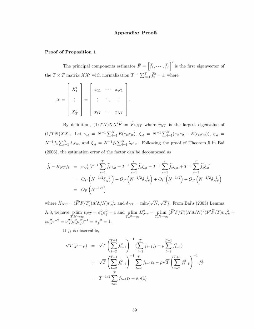
Appendix: Proofs
Proof of Proposition 1
The principal components estimator eF =h ef1; � � � ; efT i0 is the �rst eigenvector of
the T � T matrix XX 0 with normalization T�1PTt=1
ef2t = 1, where
X =
26666664X 01
...
X 0T
37777775 =26666664x11
...
x1T
� � �
. . .
� � �
xN1
...
xNT
37777775 :
By de�nition, (1=TN)XX 0 eF = eFvNT where vNT is the largest eigenvalue of
(1=TN)XX 0. Let st = N�1PNi=1E(eiseit), �st = N�1PN
i=1(eiseit � E(eiseit)), �st =
N�1fsPNi=1 �ieit, and �st = N�1ft
PNi=1 �ieis. Following the proof of Theorem 5 in Bai
(2003), the estimation error of the factor can be decomposed as
eft �HNT ft = v�1NT [T�1
TXs=1
efs st + T�1 TXs=1
efs�st + T�1 TXs=1
efs�st + T�1 TXs=1
efs�st]= OP
�N�1=2��1NT
�+OP
�N�1=2��1NT
�+OP
�N�1=2
�+OP
�N�1=2��1NT
�= OP
�N�1=2
�where HNT = ( eF 0F=T )(�0�=N)v�1NT and �NT = minfpN;pTg. From Bai�s (2003) Lemma
A.3, we have p limT;N!1
vNT = �2��2f = v and p lim
T;N!1H2NT = p lim
T;N!1( eF 0F=T )(�0�=N)2(F 0 eF=T )v�2NT =
v�2�v�2 = �2�(�
2��
2f )�1 = ��2f = 1.
If ft is observable,
pT (b�� �) =
pT
T+1Xt=2
f2t�1
!�1(TXt=2
ft�1ft � �T+1Xt=2
f2t�1)
=pT
T+1Xt=2
f2t�1
!�1 TXt=2
ft�1"t � �pT
T+1Xt=2
f2t�1
!�1f2T
= T�1=2TXt=2
ft�1"t + oP (1)
59

since T�1PTt=1 f
2t = 1 + oP (1). If ft is replaced with eft, we have
pT (e�� �) =
pT
T+1Xt=2
ef2t�1!�1
(
TXt=2
eft�1 eft � � T+1Xt=2
ef2t�1)= T�1=2
TXt=2
eft�1 � eft � � eft�1�� T�1=2� ef2T = T�1=2TXt=2
eft�1 � eft � � eft�1�+ oP (1)= T�1=2HNT
TXt=2
eft�1"t + T�1=2 TXt=2
eft�1 n eft �HNT ft � �� eft�1 �HNT ft�1�o+ oP (1)= T�1=2H2
NT
TXt=2
ft�1"t � T�1=2�TXt=2
eft�1 � eft�1 �HNT ft�1�+T�1=2
TXt=2
eft�1 � eft �HNT ft�+ T�1=2HNT TXt=2
� eft�1 �HNT ft�1� "t + oP (1):We next show (i) T�1�
PTt=2
eft�1( eft�1 � HNT ft�1) = 2�v�2N�1� + oP (��2NT );
(ii) T�1PTt=2
eft�1( eft � HNT ft) = �v�2N�1� + oP (��2NT ); and (iii) T
�1HNTPTt=2(
eft�1 �HNT ft�1)"t = oP (�
�2NT ).
We decompose the left-hand-side of (i) as,
T�1�TXt=2
eft�1( eft�1 �HNT ft�1)= T�1�
TXt=2
( eft�1 �HNT ft�1)2 + T�1� TXt=2
HNT ft�1( eft�1 �HNT ft�1)= �(A+B):
For A, we have,
A = T�1TXt=2
v�2NT [T�1
TXs=1
efs st�1 + T�1 TXs=1
efs�st�1 + T�1 TXs=1
efs�st�1 + T�1 TXs=1
efs�st�1]2= v�2NTT
�1TXt=2
(A0t +A1t +A2t +A3t)2
where A0t = T�1PTs=1
efs st�1, A1t = T�1PTs=1
efs�st�1, A2t = T�1PTs=1
efs�st�1 andA3t = T�1
PTs=1
efs�st�1.
60
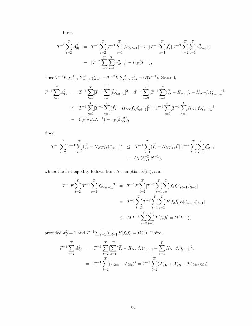
First,
T�1TXt=2
A20t = T�1TXt=2
[T�1TXs=1
efs st�1]2 � f[T�1 TXs=1
~f2s ][T�2
TXt=2
TXs=1
2st�1]g
= [T�2TXt=2
TXs=1
2st�1] = OP (T�1);
since T�2EPTt=2
PTs=1
2st�1 = T�2E
PTs=2
2ss = O(T�1). Second,
T�1TXt=2
A21t = T�1TXt=2
[T�1TXs=1
efs�st�1]2 = T�1TXt=2
[T�1TXs=1
( efs �HNT fs +HNT fs)�st�1]2� T�1
TXt=2
[T�1TXs=1
( efs �HNT fs)�st�1]2 + T�1 TXt=2
[T�1TXs=1
HNT fs�st�1]2
= OP (��2NTN
�1) = oP (��2NT );
since
T�1TXt=2
[T�1TXs=1
( efs �HNT fs)�st�1]2 � [T�1TXs=1
( efs �HNT fs)2][T�2 TXt=2
TXs=1
�2st�1]
= OP (��2NTN
�1);
where the last equality follows from Assumption E(iii), and
T�1ETXt=2
[T�1TXs=1
fs�st�1]2 = T�1E
TXt=2
[T�2TXs=1
TXl=1
fsfl�st�1� lt�1]
= T�1TXt=2
T�2TXs=1
TXl=1
E[fsfl]E[�st�1� lt�1]
� MT�2TXs=2
TXl=1
E[fsfl] = O(T�1);
provided �2f = 1 and T�1PT
s=1
PTl=1E[fsfl] = O(1). Third,
T�1TXt=2
A22t = T�3TXt=2
[TXs=1
( efs �HNT fs)�st�1 + TXs=1
HNT fs�st�1]2;
= T�1TXt=2
(A21t +A22t)2 = T�1
TXt=2
(A221t +A222t + 2A21tA22t)
61
where A21t = T�1PTs=1(
efs �HNT fs)�st�1 and A22t = T�1PTs=1HNT fs�st�1.We have
T�1TXt=2
A221t � [T�1TXs=1
( efs �HNT fs)2][T�2 TXt=2
TXs=1
�2st�1] = OP (��2NTN
�1);
where the last equality follows from
T�2ETXt=2
TXs=1
�2st�1 = T�2TXt=2
TXs=1
E(N�1fs
NXi=1
�ieit�1)2
= T�1�2f
TXt=2
N�2ENXi=1
�2i e2it�1 = O(N�1);
and
T�1TXt=2
A222t = H2NTT
�3TXt=2
(
TXs=1
fsN�1fs
NXi=1
�ieit�1)(TXs=1
fsN�1fs
NXi=1
�ieit�1)
= H2NT (T
�1TXs=1
f2s )2T�1
TXt=2
(N�1NXi=1
�ieit�1)2
= N�1� + oP (��2NT ) = OP (�
�2NT );
and
T�1TXt=2
A21tA22t � [T�1TXt=2
A21t]1=2[T�1
TXt=2
A22t]1=2 = OP (�
�2NTN
�1=2):
Therefore, T�1PTt=2A
22t = N�1� + oP (�
�2NT ) = OP (�
�2NT ). Fourth,
T�1TXt=2
A23t = T�1TXt=2
T�2[TXs=1
( efs �HNT fs)�st�1 + TXs=1
HNT fs�st�1]2;
= T�1TXt=2
(A31t +A32t)2 = T�1
TXt=2
(A231t +A232t + 2A31tA32t) = oP (�
�2NT )
where A31t = T�1PTs=1(
efs � HNT fs)�st�1 and A32t = T�1PTs=1HNT fs�st�1. The proof
of T�1PTt=1A
231t = oP (�
�2NT ) and T
�1PTt=1A31tA32t = oP (�
�2NT ) is similar to the proof of
T�1PTt=1A
221t = oP (�
�2NT ) and T
�1PTt=1A21tA22t = oP (�
�2NT ). For the remaining term,
T�1TXt=2
A232t = H2NT (T
�1TXt=2
f2t�1)(T�1
TXs=1
N�1NXi=1
fs�ieis)2 = OP ((NT )
�1);
62
since
E(T�1N�1TXs=1
NXi=1
fs�ieis)2 = E[T�2N�2
TXs=1
TXt=1
fsft
NXi=1
�2i e2is]
= M�2�E[T�2N�1
TXs=1
TXt=1
fsft] = O((NT )�1):
Using the Cauchy-Schwartz inequality, we can show that T�1PTt=2A1tA2t = oP (�
�2NT ),
T�1PTt=2A1tA3t = oP (�
�2NT ), and T�1
PTt=2A2tA3t = oP (�
�2NT ). By combining all the
results, we have A = T�1PTt=2(
eft�1 � HNT ft�1)2 = v�2NTN
�1� + oP (��2NT ) = v�2N�1� +
oP (��2NT ): For B,
B = HNT v�1NTT
�2TXt=2
TXs=1
[ft�1 efs st�1 + ft�1 efs�st�1 + ft�1 efs�st�1 + ft�1 efs�st�1]= HNT v
�1NT (B0 +B1 +B2 +B3):
First,
B0 = T�2TXt=2
TXs=1
ft�1 efs st�1 � [T�1 TXs=1
ef2s ]1=2[T�1 TXs=1
(T�1TXt=2
ft�1 st�1)2]1=2
= OP (T�1);
where
T�1ETXs=1
(T�1TXt=2
ft�1 st�1)2 = T�3E
TXs=1
T�2TXt=2
TXl=2
ft�1fl�1 st�1 sl�1
= O(T�2):
Second,
B1 = T�2TXt=2
TXs=1
ft�1 efs�st�1 � [T�1 TXs=1
ef2s ]1=2[T�1 TXs=1
(T�1TXt=2
ft�1�st�1)2]1=2
= OP ((NT )�1=2):
63
Third,
B2 = T�2TXt=2
TXs=1
ft�1 efs�st�1 � [T�1 TXs=1
ef2s ]1=2[T�1 TXs=1
(T�1TXt=2
ft�1�st�1)2]1=2
= [T�1TXs=1
ef2s ]1=2[T�1 TXs=1
(T�1TXt=2
ft�1N�1
NXi=1
fs�ieit�1)2]1=2
= [T�1TXs=1
ef2s ]1=2[(T�1 TXs=1
f2s )(T�1N�1
TXt=2
NXi=1
ft�1�ieit�1)2]1=2
= OP ((NT )�1=2):
Fourth,
B3 = T�2TXt=2
TXs=1
ft�1 efs�st�1 = T�2TXt=2
TXs=1
ft�1( efs �HNT fs +HNT fs)�st�1= T�2
TXt=2
TXs=1
ft�1( efs �HNT fs)�st�1 + T�2 TXt=2
TXs=1
ft�1HNT fs�st�1
= B31 +B32:
For B31,
B31 = [T�1TXt=2
f2t�1][T�1
TXs=1
( efs �HNT fs)N�1NXi=1
�ieis]
= T�2TXs=1
v�1NT
TXt=1
[ eft ts + eft�ts + eft�ts + eft�ts]N�1NXi=1
�ieis + oP (��2NT )
= v�1NT (B310 +B311 +B312 +B313) + oP (��2NT );
where
B310 = T�2TXs=1
TXt=1
eft tsN�1NXi=1
�ieis
� [T�1TXs=1
(T�1TXt=1
eft ts)2]1=2[T�1 TXs=1
(N�1NXi=1
�ieis)2]1=2 = OP (�
�1NTN
�1);
and
B311 = T�2TXs=1
TXt=1
eft�tsN�1NXi=1
�ieis
� [T�1TXs=1
(T�1TXt=1
eft�ts)2]1=2[T�1 TXs=1
(N�1NXi=1
�ieis)2]1=2 = OP (�
�1NTN
�1);
64
and
B312 = T�2TXs=1
TXt=1
eft�tsN�1NXi=1
�ieis = (T�1
TXt=1
eftft)[T�1 TXs=1
(N�1NXi=1
�ieis)2]
= HNTN�1� + oP (�
�2NT ):
and
B313 = T�2TXs=1
TXt=1
( eft �HNT ft +HNT ft)�tsN�1NXi=1
�ieis = OP (��1NTN
�1);
since
T�2TXs=1
TXt=1
( eft �HNT ft)�tsN�1NXi=1
�ieis
� [T�1TXt=1
( eft �HNT ft)2]1=2[T�1 TXt=1
(T�1TXs=1
�tsN�1
NXi=1
�ieis)2]1=2
� [T�1TXt=1
( eft �HNT ft)2]1=2[(T�2 TXt=1
TXs=1
�2ts)T�1
TXs=1
(N�1NXi=1
�ieis)2]1=2
= OP (��1NTN
�1T�1=2);
and
T�2TXs=1
TXt=1
HNT ft�tsN�1
NXi=1
�ieis = HNTT�2[
TXs=1
N�1NXi=1
fs�ieis]2:
= OP ((NT )�1):
Thus, B31 = HNT v�1NTN
�1� + oP (��2NT ). For B32,
B32 = T�2TXt=2
TXs=1
ft�1HNT fs�st�1 = T�2HNT
TXt=2
TXs=1
ft�1fsN�1
NXi=1
ft�1�ieis
= (T�1HNT
TXt=2
f2t�1)(T�1N�1
TXs=1
NXi=1
fs�ieis) = OP ((NT )�1=2):
Therefore, B3 = HNT v�1NTN
�1� + oP (��2NT ). By combining all the results for B1, B2 and
B3, we have B = T�1PTt=2HNT ft�1(
~ft�1 � HNT ft�1) = H2NT v
�2NTN
�1� + oP (��2NT ) =
v�2N�1�+ oP (��2NT ). Thus, T
�1�PTt=2
eft�1( eft�1�HNT ft�1) = �(A+B) = �(v�2N�1�+
v�2N�1�) + oP (��2NT ) = 2�v
�2N�1� + oP (��2NT ).
65
To show (ii), we can decompose the left-hand-side of (ii) as
T�1TXt=2
eft�1( eft�HNT ft) = T�1TXt=2
( eft�1�HNT ft�1)( eft�HNT ft)+HNTT�1 TXt=2
ft�1( eft�HNT ft):The proof is almost the same as the proof of (i). We only mention the di¤erence. To show
T�1PTt=1(
eft�1 �HNT ft�1)( eft �HNT ft) = oP (��2NT ), we need use
T�1TXt=2
( eft�1 �HNT ft�1)( eft �HNT ft)= v�2NTH
2NTT
�3TXt=2
(TXs=1
fsN�1fs
NXi=1
�ieit�1)(TXs=1
fsN�1fs
NXi=1
�ieit) + oP (��2NT )
= v�2NTH2NTT
�3(TXs=1
f2s )2TXt=2
(N�1NXi=1
�ieit�1)(N�1
NXi=1
�ieit) + oP (��2NT )
= oP (��2NT ):
To show HNTT�1PT
t=2 ft�1(eft �HNT ft) = �v�2N�1� + oP (�
�2NT ), we need use
HNTT�1
TXt=2
ft�1( eft �HNT ft) = [T�1TXt=2
ft�1ft][T�1
TXs=1
( efs �HNT fs)N�1NXi=1
�ieis] + oP (��2NT )
= �T�1TXs=1
( efs �HNT fs)N�1NXi=1
�ieis + oP (��2NT )
= �HNTN�1� + oP (�
�2NT ):
To obtain the result (iii), we �rst decompose the left-hand-side of (iii) as
T�1HNT
TXt=2
( eft�1 �HNT ft�1)"t= HNT v
�1NTT
�2TXt=2
TXs=1
[ efs st�1"t + efs�st�1"t + efs�st�1"t + efs�st�1"t]= HNT v
�1NT (C0 + C1 + C2 + C3):
For C0;
C0 = T�2TXt=2
TXs=1
efs st�1"t � (T�1 TXs=1
ef2s )1=2[T�1 TXs=1
(T�1TXt=2
st�1"t)2]1=2
= [T�1TXs=1
(T�1TXt=2
st�1"t)2]1=2 = OP ((NT )
�1=2);
66
where the last equality follows from
T�1TXs=1
E(T�1TXt=2
st�1"t)2 = T�1
TXs=1
E(T�1TXt=2
[N�1NXi=1
E(eit�1eis)]"t)2
= �2"T�3
TXs=1
TXt=2
[N�1NXi=1
E(eit�1eis)]2
= O((NT )�1):
For C1;
C1 = T�2TXt=2
TXs=1
efs�st�1"t � (T�1 TXs=1
ef2s )1=2[T�1 TXs=1
(T�1TXt=2
�st�1"t)2]1=2
= OP ((NT )�1=2);
where the last equality follows from
T�1TXs=1
E(T�1TXt=2
�st�1"t)2 = T�1
TXs=1
E(T�1TXt=2
[N�1NXi=1
(eit�1eis � E(eit�1eis))]"t)2
= �2"T�1
TXs=1
T�2ETXt=2
[N�1NXi=1
(eit�1eis � E(eit�1eis))]2
= O((NT )�1):
For C2;
C2 = T�2TXt=2
TXs=1
efs�st�1"t � (T�1 TXs=1
ef2s )1=2[T�1 TXs=1
(T�1TXt=2
�st�1"t)2]1=2 = OP ((NT )
�1=2);
where the last equality follows from
T�1TXs=1
E(T�1TXt=2
�st�1"t)2 = �2"T
�1TXs=1
E(T�2TXt=2
�2st�1)
= �2"T�1
TXs=1
E[T�2TXt=2
(N�1NXi=1
fs�ieit�1)2]
= �2"�2fT
�2E[TXt=2
(N�1NXi=1
�ieit�1)2] = O((NT )�1):
Similarly, we can show C3 = OP ((NT )�1=2): By combining all the results for C0, C1,
C2 and C3, we have T�1HNTPTt=2(
eft�1 � HNT ft�1)"t = OP ((NT )�1=2). Finally, we use
67

H2NT � 1 = oP (1) and T 1=2N�1 � c = o(1) to obtain
pT (e�� �) = T�1=2
TXt=2
ft�1"t � c�v�2� + oP (1).
The desired result follows from the central limit theorem applied to the martingale di¤erence
sequence ft�1"t with E(f2t�1"2t ) = 1� �2 combined with Slutsky�s theorem.
Proof of Proposition 2.
In this proof, we only derive the limiting behavior of E� (e�� � ~�) = E�[�PT+1
t=2ef�2t�1��1PT
t=2ef�t�1 ef�t ] � ~� based on Bootstrap Bias Correction II because the proof for Bootstrap
Bias Correction I is similar but simpler. The bootstrap principal components estimatoreF � = h ef�1 ; � � � ; ef�T i0 is the �rst eigenvector of the T � T matrix X�X�0 with normalization
T�1PTt=1
ef�2t = 1, where the bootstrap sample is given by
X� =
26666664X�01
...
X�0T
37777775 =26666664x�11
...
x�1T
� � �
. . .
� � �
x�N1
...
x�NT
37777775 :
Analogous to the original version, we have (1=TN)X�X�0 ~F � = v�NT~F � where v�NT
is the largest eigenvalue of (1=TN)X�X�0. Let ��st = N�1PNi=1 e
�ise
�it, �
�st = N�1f�s
PNi=1 �
�i e�it,
and ��st = N�1f�tPNi=1 �
�i e�is = ��ts. The estimation error of the factor can be decomposed
as
~f�t �H�NT f
�t = v��1NT T
�1TXs=1
~f�s ��st + v
��1NT T
�1TXs=1
~f�s ��st + v
��1NT T
�1TXs=1
~f�s ��st
whereH�NT = (
~F �0F �=T )(��0��=N)v��1NT . From Lemma C.1 of Gonçalves and Perron (2012),
with mutual independence of ft, �i, and eit and Ejftj8 � M , Ej�ij8 � M , Ejeitj16 � M ,
we have (a) T�1PTt=1 j eft�HNT ftj8 = OP (1); (b) N�1PN
i=1 j~�i�H�1NT�ij8 = OP (1); and (c)
(NT )�1PNi=1
PTt=1 ~e
8it = OP (1). (a), (b) and (c) imply that E�(e�8it ) = (NT )
�1PNi=1
PTt=1 ~e
8it =
68
OP (1),
E���8i = N�1NXi=1
~�8i � 8N�1(
NXi=1
j~�i �H�1NT�ij
8 +NXi=1
jH�1NT�ij
8) = OP (1);
and
E�"�8t = T�1TXt=1
( eft � ~� eft�1)8= T�1
TXt=1
[ eft �HNT ft +HNT ft � ~�( eft�1 �HNT ft�1)� ~�HNT ft�1]8� 47T�1
TXt=1
[( eft �HNT ft)8 + (HNT ft)8 + ~�4( eft�1 �HNT ft�1)8 + (~�HNT ft�1)8]= OP (1):
We denote S�T = oP �(��1T ) if the bootstrap statistic S
�T satis�es P
�(�T jS�T j > �) = oP (1) for
any � > 0 as �T !1. We have v�NT = v�+ oP �(1), where v� = �����F , �
�� =
e�0e�=N !P v
and ��F = eF 0 eF=T = 1, and H�2NT � 1 = oP �(1) because
H�2NT = ( ~F
�0F �=T )(��0��=N)2(F �0 ~F �=T )v��2NT = ���1F + op�(1):
Note that v�NT is the largest eigenvalue of a positive semi-de�nite matrix (1=TN)X�X�0 and
v�NT !P � v > 0. By the construction of our bootstrap procedure, v�NT has a lower bound
and (TN)�1X�X 0� is non-zero for all bootstrap samples. Because v�NT is greater than some
small positive number � in our bootstrap procedure, we have E�v��4NT = v�4+oP (1). Even if
there is no lower bound, P �(v�NT � �)!P 1 holds and thus the e¤ect of such a modi�cation
in our procedure on the distributions of random variables ��i , f�t , and e
�it is asymptotically
negligible. We can also show E�H�2NT = 1 + oP (1) and E�H�4
NT = 1 + oP (1) by using the
69
following argument. We have
E�[T�1TXt=1
( ~f�t�1 �H�NT f
�t�1)
2]
= T�1E�fTXt=1
v��2NT [T�1
TXs=1
ef�s ��st�1 + T�1 TXs=1
ef�s ��st�1 + T�1 TXs=1
ef�s ��st�1]2g= v��2NT E
�fT�1TXt=1
(A�1t +A�2t +A
�3t)
2g
� ��2E�fT�1TXt=1
(A�1t +A�2t +A
�3t)
2g;
where A�1t = T�1PTs=1
ef�s ��st�1, A�2t = T�1PTs=1
ef�s ��st�1 and A�3t = T�1PTs=1
ef�s ��st�1.First,
E�fT�1TXt=1
A�21t g = E�fT�1TXt=1
[T�1TXs=1
ef�s ��st�1]2g� E�f[T�1
TXs=1
ef�2s ][T�2 TXt=1
TXs=1
��2st�1]g
= fE�[T�2TXt=1
TXs=1
��2st�1]g = T�2TXt=1
TXs=1
N�2E�[NXi=1
e�2is e�2it ]
= OP (��2NT );
provided E�e�4it = OP (1): Second,
E�fT�1TXt=1
A�22t g = E�fT�1TXt=1
(T�1TXs=1
~f�sN�1f�s
NXi=1
��i e�it�1)
2g
= E�fT�1TXt=1
(T�1TXs=1
~f�s f�s )2(N�1
NXi=1
��i e�it)2g
� E�f(T�1TXs=1
~f�2s )(T�1
TXs=1
f�2s )T�1
TXt=1
(N�1NXi=1
��i e�it)2g
= E�[(T�1TXs=1
f�2s )][T�1
TXt=1
N�2E�NXi=1
��2i e�2it ]
= E�[(T�1TXs=1
f�2s )][T�1
TXt=1
N�2NXi=1
E���2i E�e�2it ]
= OP (��2NT );
70
which follows from E�[T�1PTs=1 f
�2s ] = T�1
PTs=1
~f2s = 1 and E���4i = OP (1). Third,
E�fT�1TXt=1
A�23t g = E�f(T�1TXt=1
f�2t )(T�1
TXs=1
~f�sN�1
NXi=1
��i e�is)2g
� E�f(T�1TXs=1
~f�2s )(T�1
TXt=1
f�2t )[T�1
TXs=1
(N�1NXi=1
��i e�is)2]g
= fE�(T�1TXt=1
f�2t )[T�1N�2E�
TXs=1
NXi=1
��2i e�2is ]g
= OP (��2NT ):
Using the Cauchy-Schwartz inequality, we can show that E�[T�1PTt=1A
�1tA
�2t] = OP (�
�2NT ),
E�[T�1PTt=1A
�1tA
�3t] = OP (�
�2NT ), and E
�[T�1PTt=1A
�2tA
�3t] = OP (�
�2NT ). Therefore, we
have E�[T�1PTt=1(
~f�t�1�H�NT f
�t�1)
2] = OP (��2NT ). Since H
�2NT = 1+ oP �(1); with Markov�s
inequality we have E�H�2NT � 1 + oP (1): Also, with E�[T�1
PTt=1(
~f�t�1 � H�NT f
�t�1)
2] =
OP (��2NT ),
E�H�2NT = E�[T�1 ~F �
0 ~F � T�1( ~F � �H�NT
~F )0 ~F ]2
= E�(T�1 ~F �0 ~F )2 + E�[T�1( ~F � �H�
NT~F )0 ~F ]2 � 2E�[T�2 ~F �0 ~F ( ~F � �H�
NT~F )0 ~F ]
� E�(T�1jj ~F �0 jjjj ~F jj) + oP (1) = 1 + oP (1):
Therefore, E�H�2NT = 1+ oP (1):Similarly, with E
�e�8it , E���8i , and E
�"�8i bounded in proba-
bility, we can obtain E�[T�1PTt=1(
~f�t�1�H�NT f
�t�1)
4] = OP (��4NT ) and E
�H�4NT = 1+oP (1).
71
The bootstrap bias estimator can be decomposed as
E� (e�� � ~�)= E�[
T+1Xt=2
ef�2t�1!�1
(TXt=2
ef�t�1 ef�t � ~� T+1Xt=2
ef�2t�1)]= T�1E�[
TXt=2
ef�t�1 � ef�t � ~� ef�t�1�]� T�1~�E� ef�2T= T�1E�[
TXt=2
ef�t�1 � ef�t � ~� ef�t�1�] + oP (T�1=2)= T�1E�[
TXt=2
ef�t�1 n ef�t �H�NT f
�t � ~�
� ef�t�1 �H�NT f
�t�1
�o+H�
NT
TXt=2
ef�t�1"�t ] + oP (T�1=2)= T�1E�[H�2
NT
TXt=2
f�t�1"�t ]� T�1E�[~�
TXt=2
ef�t�1 � ef�t�1 �H�NT f
�t�1
�]
+T�1E�[TXt=2
ef�t�1 � ef�t �H�NT f
�t
�] + T�1E�[H�
NT
TXt=2
� ef�t�1 �H�NT f
�t�1
�"�t ] + oP (T
�1=2):
Note that third equality follows from T�1E� ef�2T = oP (T�1=2) which can be shown by using
the decomposition T�1E�H�2NT f
�2T +T
�1E�( ef�T�H�NT f
�T )2. The leading term can be written
as
T�1E�[�H�2NT � 1
� TXt=2
f�t�1"�t +
TXt=2
f�t�1"�t ] = T�1E�[
�H�2NT � 1
� TXt=2
f�t�1"�t ]
� fE�[H�4NT � 2H�2
NT + 1]T�2E�[
TXt=2
f�t�1"�t ]2g1=2
= fE�[H�2NT � 1]2T�2E�[
TXt=2
f�2t�1"�2t ]g1=2 = oP (T
�1=2);
where we use the fact E�[H�2NT�1]2 = oP (1). In what follows, we show that (i) T�1E�[~�
PTt=2
ef�t�1� ef�t�1 �H�NT f
�t�1
�] = 2N�1�v�2� + oP (T
�1=2); (ii) T�1E�[~�PTt=2
ef�t�1 � ef�t �H�NT f
�t
�] =
N�1�v�2�+oP (T�1=2); and (iii) T�1E�[H�
NT
PTt=2(
ef�t�1� H�NT f
�t�1)"
�t = oP (T
�1=2). The
proof of (i) to (iii) is similar to the proof of Proposition 1. For (i),
T�1E�f~�TXt=2
~f�t�1( ~f�t�1 �H�
NT f�t�1)g = ~�(A� +B�)
72
where A� = E�fT�1PTt=2(
~f�t�1�H�NT f
�t�1)
2g = v��2NT E�fT�1
PTt=1(A
�1t+A
�2t+A
�3t)
2g and
B� = E�fT�1PTt=2H
�NT f
�t�1(
~f�t�1 � H�NT f
�t�1)g. To show A� = v�2N�1� + oP (�
�2NT ), we
can focus on dominant term A�2t which is analogous to the dominant term A2t in the proof
of Proposition 1.
E�fv��2NT T�1
TXt=2
A�22t g = T�3E�v��2NT
TXt=2
[TXs=1
( ef�s �H�NT f
�s )�
�st�1 +
TXs=1
H�NT f
�s ��st�1]
2;
= T�1E�v��2NT
TXt=2
(A�21t +A�22t)
2
= T�1E�v��2NT
TXt=2
(A�221t +A�222t + 2A
�21tA
�22t);
where A�21t = T�1PTs=1(
ef�s � H�NT f
�s )�
�st�1 and A
�22t = T�1
PTs=1H
�NT f
�s ��st�1. Further-
more,
T�1E�v��2NT
TXt=2
A�221t � ��2E�f[T�1TXs=1
( ef�s �H�NT f
�s )2][T�2
TXt=2
TXs=1
��2st�1]g
= ��2fE�[T�1TXs=1
( ef�s �H�NT f
�s )2]2E�[T�2
TXt=2
TXs=1
��2st�1]2g1=2
= OP ((TN)�1=2);
and
T�1E�v��2NT
TXt=2
A�222t = T�1E�(v��2NT H�2NT �v�2)H��2
NT
TXt=2
A�222t+T�1E�v�2H��2
NT
TXt=2
A�222t;
where
T�1E�v�2H��2NT
TXt=2
A�222t = v�2E�[T�3TXt=2
(
TXs=1
f�sN�1f�s
NXi=1
��i e�it�1)
2]
= E�fv�2(T�1TXs=1
f�2s )2T�1
TXt=2
(N�1NXi=1
��i e�it�1)
2g
= v�2E�(T�1TXs=1
f�2s )2E�[T�1
TXt=2
(N�1NXi=1
��i e�it�1)
2]
= v�2N�1� + oP (T�1=2) = OP (�
�2NT );
73
where the last equality follows from
T�1E�TXt=2
(N�1=2NXi=1
��i e�it)2 = T�1N�1
TXt=2
NXi=1
e�2i ee2it= � + oP (1);
and
T�1E�(v��2NT H�2NT � v�2)H��2
NT
TXt=2
A�222t
= E�(v��2NT H�2NT � v�2)[T�3
TXs=1
f�2s
TXt=2
(N�1NXi=1
��i e�it�1)
2]
� E�(v��2NT H�2NT � v�2)2E�[T�3
TXs=1
f�2s
TXt=2
(N�1NXi=1
��i e�it�1)
2]2
= oP (��2NT );
and
T�1E�v��2NT
TXt=2
A�21tA�22t � E�fv��2NT [T
�1TXt=2
A�221t]1=2[T�1
TXt=2
A�222t]1=2g
� ��2fE�[T�1TXt=2
A�221t]E�[T�1
TXt=2
A�222t]g1=2 = oP (��2NT ):
Therefore, T�1E�v��2NT
PTt=2A
�22t = v�2N�1� + oP (�
�2NT ) = OP (�
�2NT ). By combining all the
results, A� = v�2N�1� + oP (��2NT ): For B
�, we have
B� = E�fH�NT v
��1NT T
�2TXt=2
TXs=1
[f�t�1 ef�s ��st�1 + f�t�1 ef�s ��st�1 + f�t�1 ef�s ��st�1]g= (B�1 +B
�2 +B
�3):
74
First,
B�1 = T�2E�[H�NT v
��1NT
TXt=2
TXs=1
f�t�1 ef�s ��st�1]� E�f[T�1H�
NT v��2NT
TXs=1
ef�2s ]1=2[T�1 TXs=1
(T�1TXt=2
f�t�1��st�1)
2]1=2g
= E�f[H�NT v
��2NT ][T
�1TXs=1
(T�1TXt=2
f�t�1N�1
NXi=1
e�ise�it�1)
2]g1=2
� f��2E�[H�2NT ]E
�[T�1TXs=1
(T�1TXt=2
f�t�1N�1
NXi=1
e�ise�it�1)
2]g1=2
= OP ((NT )�1=2):
Second,
B�2 = T�2E�[H�NT v
��1NT
TXt=2
TXs=1
f�t�1 ef�s ��st�1]� E�f[H�2
NT v��2NT T
�1TXs=1
ef�2s ][T�1 TXs=1
(T�1TXt=2
TXs=1
f�t�1��st�1)
2]g1=2
= E�fH�2NT v
��2NT [T
�1TXs=1
(T�1TXt=2
f�t�1��st�1)
2]g1=2
� f��2E�[H�2NT ]E
�[T�1TXs=1
(T�1TXt=2
f�t�1��st�1)
2]g1=2
= OP ((NT )�1=2):
Third,
B�3 = T�2E�[H�NT v
��1NT
TXt=2
TXs=1
f�t�1 ef�s ��st�1]= T�2E[H�
NT v��1NT
TXt=2
TXs=1
f�t�1( ef�s �H�NT f
�s +H
�NT f
�s )�
�st�1]
= T�2E�fH�NT v
��1NT [
TXt=2
TXs=1
f�t�1( ef�s �H�NT f
�s )�
�st�1 +
TXt=2
TXs=1
f�t�1H�NT f
�s ��st�1]g
= B�31 +B�32:
75
For B�31,
B�31 = E�fH�NT v
��1NT [T
�1TXt=2
f�2t�1][T�1
TXs=1
( ef�s �H�NT f
�s )N
�1NXi=1
��i e�is]g
= T�2E�fTXs=1
H�NT v
��2NT
TXt=1
[ ef�t ��ts + ef�t ��ts + ef�t ��ts]N�1NXi=1
��i e�isg
= (B�311 +B�312 +B
�313);
where
B�311 = T�2E�[H�NT v
��2NT
TXs=1
TXt=1
ef�t ��tsN�1NXi=1
��i e�is]
� E�f[(T�1H�NT v
��2NT
TXt=1
ef�t )2]1=2[T�3 TXt=1
(TXs=1
��tsN�1
NXi=1
��i e�is)2]1=2g
� E�f[H�2NT v
��4NT ]
1=2[T�3TXt=1
(
TXs=1
��tsN�1
NXi=1
��i e�is)2]1=2g
� ��2fE�f[H�2NT ]E
�[T�1TXt=1
(T�1TXs=1
��tsN�1
NXi=1
��i e�is)2]g1=2
= OP ((NT )�1=2);
and
B�312 = E�[H�NT v
��2NT T
�2TXs=1
TXt=1
ef�t ��tsN�1NXi=1
��i e�is]
= E�fH�NT v
��2NT (T
�1TXt=1
ef�t f�t )[T�1 TXs=1
(N�1NXi=1
��i e�is)2]g
= E�fv�2(T�1TXt=1
f�2t )[T�1
TXs=1
(N�1NXi=1
��i e�is)2]g
+E�f(H�2NT v
��2NT � v
�2)(T�1TXt=1
f�2t )[T�1
TXs=1
(N�1NXi=1
��i e�is)2]g
+EfH�NT v
�2NT [T
�1TXt=1
( ef�t �H�NT f
�t )f
�t ][T
�1TXs=1
(N�1NXi=1
��i e�is)2]g
= v�2N�1� + oP (��2NT ) + oP (�
�2NT );
76
and
B�313 = T�2E[H�NT v
��2NT
TXs=1
TXt=1
( ef�t �H�NT f
�t +H
�NT f
�t )�
�tsN
�1NXi=1
��i e�is]
= OP (��1NTN
�1);
since
T�2E�[H�NT v
��2NT
TXs=1
TXt=1
( ef�t �H�NT f
�t )�
�tsN
�1NXi=1
��i e�is]
� E�f[H�2NT v
��4NT T
�1TXt=1
( ef�t �H�NT f
�t )2]1=2[T�1
TXt=1
(T�1TXs=1
��tsN�1
NXi=1
��i e�is)2]1=2g
� fE�[T�1H�2NT v
��4NT
TXt=1
( ef�t �H�NT f
�t )2]E�[T�1
TXt=1
(T�1TXs=1
��tsN�1
NXi=1
��i e�is)2]g1=2
� ��2fE�[T�1H�2NT
TXt=1
( ef�t �H�NT f
�t )2]E�[T�1
TXt=1
(T�1TXs=1
��tsN�1
NXi=1
��i e�is)2]g1=2
� ��2fE�H�4NTE
�[T�1TXt=1
( ef�t �H�NT f
�t )2]2E�[T�1
TXt=1
(T�1TXs=1
��tsN�1
NXi=1
��i e�is)2]g1=2
= OP ((NT )�1=2);
and
T�2E�[H�2NT v
��2NT
TXs=1
TXt=1
f�t ��tsN
�1NXi=1
��i e�is]
= E�fH�2NT v
��2NT [T
�1TXs=1
N�1NXi=1
f�s ��i e�is]2g: = OP ((NT )
�1=2):
Thus, B�31 = v�2N�1� + oP (��2NT ). For B
�32,
B�32 = E�[H�2NT v
��1NT T
�2TXt=2
TXs=1
f�t�1f�s ��st�1]
= E�[H�2NT v
��1NT T
�2TXt=2
TXs=1
f�t�1f�sN
�1NXi=1
f�t�1��i e�is]
= E�[H�2NT v
��1NT (T
�1TXt=2
f�2t�1)(T�1N�1
TXs=1
NXi=1
f�s ��i e�is)] = OP ((NT )
�1=2):
Therefore, B�3 = v�2N�1�+ oP (��2NT ). By combining all the results for B
�1 , B
�2 and B
�3 , we
haveB� = v�2N�1�+oP (��2NT ). Thus, E
�[T�1~�PTt=2
ef�t�1( ef�t�1�H�NT f
�t�1)] = ~�(A
�+B�) =
77
2�v�2N�1� + oP (��2NT ) which completes the proof of (i).
To show (ii), we use a similar decomposition as (i),
T�1E�~�TXt=2
ef�t�1( ef�t �H�NT f
�t )
= E�[T�1~�TXt=2
( ef�t�1 �H�NT f
�t�1)( ef�t �H�
NT f�t ) + T
�1H�NT ~�
TXt=2
f�t�1( ef�t �H�NT f
�t )]:
Since the proof is almost the same as the proof of (i), we only mention the di¤erence. To
show T�1E�PTt=2(
ef�t�1 �H�NT f
�t�1)(
ef�t �H�NT f
�t ) = oP (�
�2NT ), we need to use
T�1E�TXt=2
( ef�t�1 �H�NT f
�t�1)( ef�t �H�
NT f�t )
= E�[H�2NT v
��2NT T
�3TXt=2
(TXs=1
f�sN�1f�s
NXi=1
��i e�it�1)(
TXs=1
f�sN�1f�s
NXi=1
��i e�it)] + oP (�
�2NT )
= E�[H�2NT v
��2NT T
�3(TXs=1
f�2s )2TXt=1
(N�1NXi=1
��i e�it�1)(N
�1NXi=1
��i e�it)] + oP (�
�2NT )
= oP (��2NT ):
To show E�[H�NTT
�1PTt=2 f
�t�1(
ef�t �H�NT f
�t )] = �v�2N�1� + oP (�
�2NT ), we need to use
E�[H�NTT
�1TXt=2
f�t�1( ef�t �H�NT f
�t )]
= E�f[T�1TXt=2
f�t�1f�t ][T
�1TXs=1
( ef�s �H�NT f
�s )N
�1NXi=1
��i e�is]g+ oP (��2NT )
= E�[~�[T�1TXt=2
f�2t�1]T�1
TXs=1
( ef�s �H�NT f
�s )N
�1NXi=1
��i e�is] + oP (�
�2NT )
= �v�2N�1� + oP (��2NT ):
To obtain the result (iii), we have
T�1E�[H�NT
TXt=2
( ef�t�1 �H�NT f
�t�1)"
�t ]
= E�fH�NT v
��1NT T
�2TXt=2
TXs=1
[ ef�s ��st�1"�t + ef�s ��st�1"�t + ef�s ��st�1"�t ]g= C�1 + C
�2 + C
�3 :
78
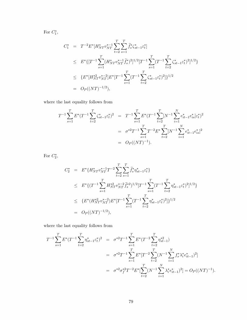
For C�1 ;
C�1 = T�2E�[H�NT v
��1NT
TXt=2
TXs=1
ef�s ��st�1"�t ]� E�f[T�1
TXs=1
(H�NT v
��1NT
ef�s )2]1=2[T�1 TXs=1
(T�1TXt=2
��st�1"�t )2]1=2g
� fE�[H�2NT v
��2NT ]E
�[T�1TXs=1
(T�1TXt=2
��st�1"�t )2]g1=2
= OP ((NT )�1=2);
where the last equality follows from
T�1TXs=1
E�(T�1TXt=2
��st�1"�t )2 = T�1
TXs=1
E�(T�1TXt=2
[N�1NXi=1
e�it�1e�is]"
�t )2
= ��2T�1TXs=1
T�2E�TXt=2
[N�1NXi=1
e�it�1e�is]2
= OP ((NT )�1):
For C�2 ;
C�2 = E�fH�NT v
��1NT T
�2TXt=2
TXs=1
ef�s ��st�1"�t g� E�f(T�1
TXs=1
H�2NT v
��2NT
ef�2s )1=2[T�1 TXs=1
(T�1TXt=2
��st�1"�t )2]1=2g
� fE�(H�2NT v
��2NT )E
�[T�1TXs=1
(T�1TXt=2
��st�1"�t )2]g1=2
= OP ((NT )�1=2);
where the last equality follows from
T�1TXs=1
E�(T�1TXt=2
��st�1"�t )2 = ��2T�1
TXs=1
E�(T�2TXt=2
��2st�1)
= ��2T�1TXs=1
E�[T�2TXt=2
(N�1NXi=1
f�s ��i e�it�1)
2]
= ��2��2f T�2E�[
TXt=2
(N�1NXi=1
��i e�it�1)
2] = OP ((NT )�1):
79
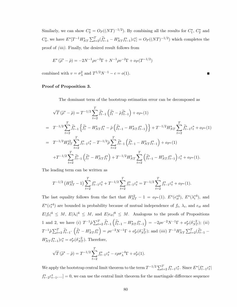
Similarly, we can show C�3 = OP ((NT )�1=2): By combining all the results for C�1 , C
�2 and
C�3 , we have E�[T�1H�
NT
PTt=2(
ef�t�1 �H�NT f
�t�1)"
�t ] = OP ((NT )
�1=2) which completes the
proof of (iii). Finally, the desired result follows from
E� (e�� � ~�) = �2N�1�v�2� +N�1�v�2� + oP (T�1=2)
combined with v = �2� and T1=2N�1 � c = o(1).
Proof of Proposition 3.
The dominant term of the bootstrap estimation error can be decomposed as
pT (e�� � ~�) = T�1=2
TXt=2
ef�t�1 � ef�t � ~� ef�t�1�+ oP �(1)= T�1=2
TXt=2
ef�t�1 n ef�t �H�NT f
�t � ~�
� ef�t�1 �H�NT f
�t�1
�o+ T�1=2H�
NT
TXt=2
ef�t�1"�t + oP �(1)= T�1=2H�2
NT
TXt=2
f�t�1"�t � T�1=2~�
TXt=2
ef�t�1 � ef�t�1 �H�NT f
�t�1
�+ oP �(1)
+T�1=2TXt=2
ef�t�1 � ef�t �H�NT f
�t
�+ T�1=2H�
NT
TXt=2
� ef�t�1 �H�NT f
�t�1
�"�t + oP �(1):
The leading term can be written as
T�1=2�H�2NT � 1
� TXt=2
f�t�1"�t + T
�1=2TXt=2
f�t�1"�t = T�1=2
TXt=2
f�t�1"�t + oP �(1).
The last equality follows from the fact that H�2NT � 1 = oP �(1): E
�(e�4it ), E�(��4i ), and
E�("�4t ) are bounded in probability because of mutual independence of ft, �i, and eit and
Ejftj4 � M , Ej�ij4 � M , and Ejeitj8 � M . Analogous to the proofs of Propositions
1 and 2, we have (i) T�1~�PTt=2
ef�t�1 � ef�t�1 �H�NT f
�t�1
�= �2�v�2N�1� + o�P (�
�2NT ); (ii)
T�1~�PTt=2
ef�t�1� � ef�t �H�NT f
�t
�= �v�2N�1� + o�P (�
�2NT ); and (iii) T
�1H�NT
PTt=2(
ef�t�1 �H�NT f
�t�1)"
�t = o�P (�
�2NT ): Therefore,
pT (e�� � ~�) = T�1=2
TXt=2
f�t�1"�t � c���4� � + o
�P (1):
We apply the bootstrap central limit theorem to the term T�1=2PTt=2 f
�t�1"
�t . Since E
�[f�t�1"�t j
f�t�2"�t�1; :::] = 0, we can use the central limit theorem for the martingale di¤erence sequence
80

under the bootstrap probability measure and thus P �(pT (~�� � ~�) � x) approaches normal
distribution function with mean �c���4� � and variance E�(f�2t�1"�2t ) = T�1PTt=2
~f2t�1~"2t un-
der the bootstrap probability measure. Combining it with T�1PTt=2
~f2t�1~"2t !P E(f2t�1"
2t ) =
1� �2, we have P �(pT (~��� ~�) � x)�P (
pT (~�� �) � x)!P 0 for any x. By using Polya�s
theorem, we have the uniform convergence result.
81
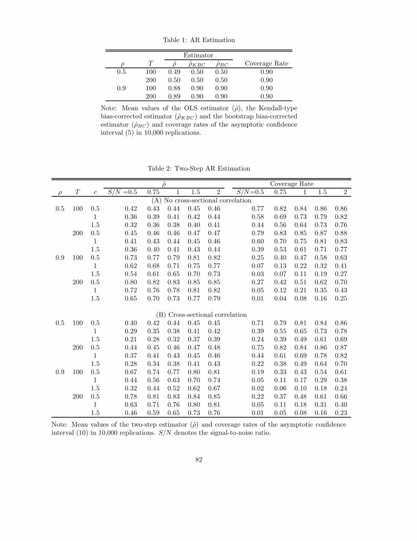
Table 1: AR Estimation
Estimatorρ T ρ ρKBC ρBC Coverage Rate
0.5 100 0.49 0.50 0.50 0.90200 0.50 0.50 0.50 0.90
0.9 100 0.88 0.90 0.90 0.90200 0.89 0.90 0.90 0.90
Note: Mean values of the OLS estimator (ρ), the Kendall-typebias-corrected estimator (ρKBC) and the bootstrap bias-correctedestimator (ρBC) and coverage rates of the asymptotic confidenceinterval (5) in 10,000 replications.
Table 2: Two-Step AR Estimation
ρ Coverage Rateρ T c S/N =0.5 0.75 1 1.5 2 S/N=0.5 0.75 1 1.5 2
(A) No cross-sectional correlation0.5 100 0.5 0.42 0.43 0.44 0.45 0.46 0.77 0.82 0.84 0.86 0.86
1 0.36 0.39 0.41 0.42 0.44 0.58 0.69 0.73 0.79 0.821.5 0.32 0.36 0.38 0.40 0.41 0.44 0.56 0.64 0.73 0.76
200 0.5 0.45 0.46 0.46 0.47 0.47 0.79 0.83 0.85 0.87 0.881 0.41 0.43 0.44 0.45 0.46 0.60 0.70 0.75 0.81 0.83
1.5 0.36 0.40 0.41 0.43 0.44 0.39 0.53 0.61 0.71 0.770.9 100 0.5 0.73 0.77 0.79 0.81 0.82 0.25 0.40 0.47 0.58 0.63
1 0.62 0.68 0.71 0.75 0.77 0.07 0.13 0.22 0.32 0.411.5 0.54 0.61 0.65 0.70 0.73 0.03 0.07 0.11 0.19 0.27
200 0.5 0.80 0.82 0.83 0.85 0.85 0.27 0.42 0.51 0.62 0.701 0.72 0.76 0.78 0.81 0.82 0.05 0.12 0.21 0.35 0.43
1.5 0.65 0.70 0.73 0.77 0.79 0.01 0.04 0.08 0.16 0.25
(B) Cross-sectional correlation0.5 100 0.5 0.40 0.42 0.44 0.45 0.45 0.71 0.79 0.81 0.84 0.86
1 0.29 0.35 0.38 0.41 0.42 0.39 0.55 0.65 0.73 0.781.5 0.21 0.28 0.32 0.37 0.39 0.24 0.39 0.49 0.61 0.69
200 0.5 0.44 0.45 0.46 0.47 0.48 0.75 0.82 0.84 0.86 0.871 0.37 0.41 0.43 0.45 0.46 0.44 0.61 0.69 0.78 0.82
1.5 0.28 0.34 0.38 0.41 0.43 0.22 0.38 0.49 0.64 0.700.9 100 0.5 0.67 0.74 0.77 0.80 0.81 0.19 0.33 0.43 0.54 0.61
1 0.44 0.56 0.63 0.70 0.74 0.05 0.11 0.17 0.29 0.381.5 0.32 0.44 0.52 0.62 0.67 0.02 0.06 0.10 0.18 0.24
200 0.5 0.78 0.81 0.83 0.84 0.85 0.22 0.37 0.48 0.61 0.661 0.63 0.71 0.76 0.80 0.81 0.05 0.11 0.18 0.31 0.40
1.5 0.46 0.59 0.65 0.73 0.76 0.01 0.05 0.08 0.16 0.23
Note: Mean values of the two-step estimator (ρ) and coverage rates of the asymptotic confidenceinterval (10) in 10,000 replications. S/N denotes the signal-to-noise ratio.
82
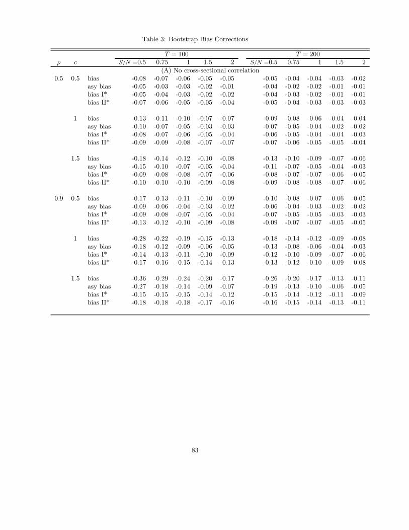
Table 3: Bootstrap Bias Corrections
T = 100 T = 200ρ c S/N =0.5 0.75 1 1.5 2 S/N =0.5 0.75 1 1.5 2
(A) No cross-sectional correlation0.5 0.5 bias -0.08 -0.07 -0.06 -0.05 -0.05 -0.05 -0.04 -0.04 -0.03 -0.02
asy bias -0.05 -0.03 -0.03 -0.02 -0.01 -0.04 -0.02 -0.02 -0.01 -0.01bias I* -0.05 -0.04 -0.03 -0.02 -0.02 -0.04 -0.03 -0.02 -0.01 -0.01bias II* -0.07 -0.06 -0.05 -0.05 -0.04 -0.05 -0.04 -0.03 -0.03 -0.03
1 bias -0.13 -0.11 -0.10 -0.07 -0.07 -0.09 -0.08 -0.06 -0.04 -0.04asy bias -0.10 -0.07 -0.05 -0.03 -0.03 -0.07 -0.05 -0.04 -0.02 -0.02bias I* -0.08 -0.07 -0.06 -0.05 -0.04 -0.06 -0.05 -0.04 -0.04 -0.03bias II* -0.09 -0.09 -0.08 -0.07 -0.07 -0.07 -0.06 -0.05 -0.05 -0.04
1.5 bias -0.18 -0.14 -0.12 -0.10 -0.08 -0.13 -0.10 -0.09 -0.07 -0.06asy bias -0.15 -0.10 -0.07 -0.05 -0.04 -0.11 -0.07 -0.05 -0.04 -0.03bias I* -0.09 -0.08 -0.08 -0.07 -0.06 -0.08 -0.07 -0.07 -0.06 -0.05bias II* -0.10 -0.10 -0.10 -0.09 -0.08 -0.09 -0.08 -0.08 -0.07 -0.06
0.9 0.5 bias -0.17 -0.13 -0.11 -0.10 -0.09 -0.10 -0.08 -0.07 -0.06 -0.05asy bias -0.09 -0.06 -0.04 -0.03 -0.02 -0.06 -0.04 -0.03 -0.02 -0.02bias I* -0.09 -0.08 -0.07 -0.05 -0.04 -0.07 -0.05 -0.05 -0.03 -0.03bias II* -0.13 -0.12 -0.10 -0.09 -0.08 -0.09 -0.07 -0.07 -0.05 -0.05
1 bias -0.28 -0.22 -0.19 -0.15 -0.13 -0.18 -0.14 -0.12 -0.09 -0.08asy bias -0.18 -0.12 -0.09 -0.06 -0.05 -0.13 -0.08 -0.06 -0.04 -0.03bias I* -0.14 -0.13 -0.11 -0.10 -0.09 -0.12 -0.10 -0.09 -0.07 -0.06bias II* -0.17 -0.16 -0.15 -0.14 -0.13 -0.13 -0.12 -0.10 -0.09 -0.08
1.5 bias -0.36 -0.29 -0.24 -0.20 -0.17 -0.26 -0.20 -0.17 -0.13 -0.11asy bias -0.27 -0.18 -0.14 -0.09 -0.07 -0.19 -0.13 -0.10 -0.06 -0.05bias I* -0.15 -0.15 -0.15 -0.14 -0.12 -0.15 -0.14 -0.12 -0.11 -0.09bias II* -0.18 -0.18 -0.18 -0.17 -0.16 -0.16 -0.15 -0.14 -0.13 -0.11
83
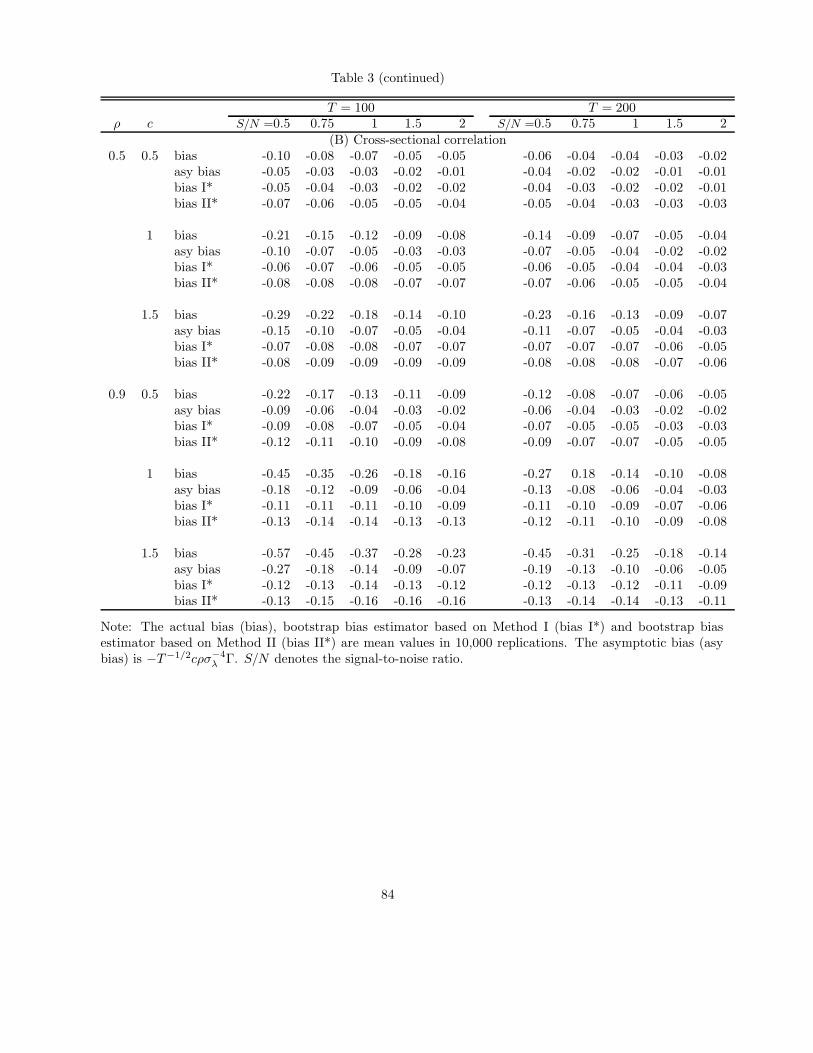
Table 3 (continued)
T = 100 T = 200ρ c S/N =0.5 0.75 1 1.5 2 S/N =0.5 0.75 1 1.5 2
(B) Cross-sectional correlation0.5 0.5 bias -0.10 -0.08 -0.07 -0.05 -0.05 -0.06 -0.04 -0.04 -0.03 -0.02
asy bias -0.05 -0.03 -0.03 -0.02 -0.01 -0.04 -0.02 -0.02 -0.01 -0.01bias I* -0.05 -0.04 -0.03 -0.02 -0.02 -0.04 -0.03 -0.02 -0.02 -0.01bias II* -0.07 -0.06 -0.05 -0.05 -0.04 -0.05 -0.04 -0.03 -0.03 -0.03
1 bias -0.21 -0.15 -0.12 -0.09 -0.08 -0.14 -0.09 -0.07 -0.05 -0.04asy bias -0.10 -0.07 -0.05 -0.03 -0.03 -0.07 -0.05 -0.04 -0.02 -0.02bias I* -0.06 -0.07 -0.06 -0.05 -0.05 -0.06 -0.05 -0.04 -0.04 -0.03bias II* -0.08 -0.08 -0.08 -0.07 -0.07 -0.07 -0.06 -0.05 -0.05 -0.04
1.5 bias -0.29 -0.22 -0.18 -0.14 -0.10 -0.23 -0.16 -0.13 -0.09 -0.07asy bias -0.15 -0.10 -0.07 -0.05 -0.04 -0.11 -0.07 -0.05 -0.04 -0.03bias I* -0.07 -0.08 -0.08 -0.07 -0.07 -0.07 -0.07 -0.07 -0.06 -0.05bias II* -0.08 -0.09 -0.09 -0.09 -0.09 -0.08 -0.08 -0.08 -0.07 -0.06
0.9 0.5 bias -0.22 -0.17 -0.13 -0.11 -0.09 -0.12 -0.08 -0.07 -0.06 -0.05asy bias -0.09 -0.06 -0.04 -0.03 -0.02 -0.06 -0.04 -0.03 -0.02 -0.02bias I* -0.09 -0.08 -0.07 -0.05 -0.04 -0.07 -0.05 -0.05 -0.03 -0.03bias II* -0.12 -0.11 -0.10 -0.09 -0.08 -0.09 -0.07 -0.07 -0.05 -0.05
1 bias -0.45 -0.35 -0.26 -0.18 -0.16 -0.27 0.18 -0.14 -0.10 -0.08asy bias -0.18 -0.12 -0.09 -0.06 -0.04 -0.13 -0.08 -0.06 -0.04 -0.03bias I* -0.11 -0.11 -0.11 -0.10 -0.09 -0.11 -0.10 -0.09 -0.07 -0.06bias II* -0.13 -0.14 -0.14 -0.13 -0.13 -0.12 -0.11 -0.10 -0.09 -0.08
1.5 bias -0.57 -0.45 -0.37 -0.28 -0.23 -0.45 -0.31 -0.25 -0.18 -0.14asy bias -0.27 -0.18 -0.14 -0.09 -0.07 -0.19 -0.13 -0.10 -0.06 -0.05bias I* -0.12 -0.13 -0.14 -0.13 -0.12 -0.12 -0.13 -0.12 -0.11 -0.09bias II* -0.13 -0.15 -0.16 -0.16 -0.16 -0.13 -0.14 -0.14 -0.13 -0.11
Note: The actual bias (bias), bootstrap bias estimator based on Method I (bias I*) and bootstrap biasestimator based on Method II (bias II*) are mean values in 10,000 replications. The asymptotic bias (asybias) is −T−1/2cρσ−4
λ Γ. S/N denotes the signal-to-noise ratio.
84
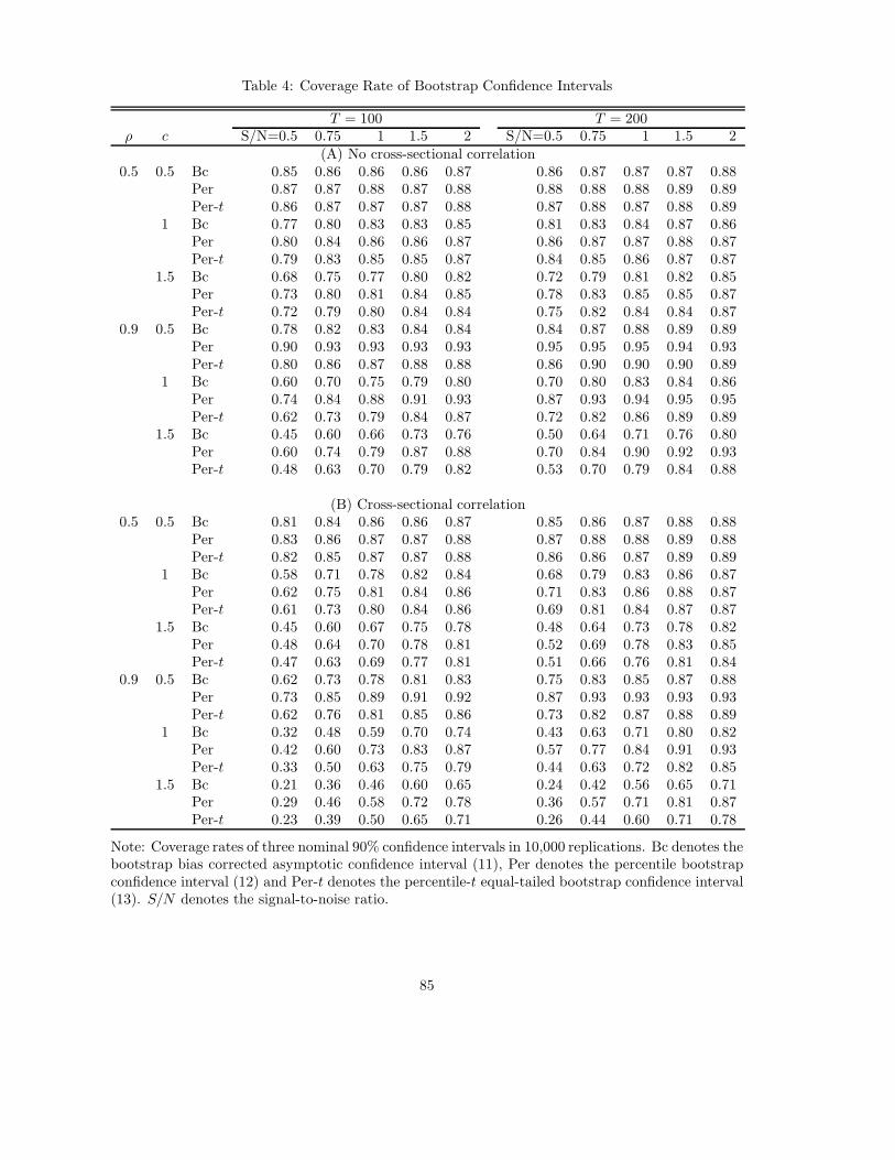
Table 4: Coverage Rate of Bootstrap Confidence Intervals
T = 100 T = 200ρ c S/N=0.5 0.75 1 1.5 2 S/N=0.5 0.75 1 1.5 2
(A) No cross-sectional correlation0.5 0.5 Bc 0.85 0.86 0.86 0.86 0.87 0.86 0.87 0.87 0.87 0.88
Per 0.87 0.87 0.88 0.87 0.88 0.88 0.88 0.88 0.89 0.89Per-t 0.86 0.87 0.87 0.87 0.88 0.87 0.88 0.87 0.88 0.89
1 Bc 0.77 0.80 0.83 0.83 0.85 0.81 0.83 0.84 0.87 0.86Per 0.80 0.84 0.86 0.86 0.87 0.86 0.87 0.87 0.88 0.87Per-t 0.79 0.83 0.85 0.85 0.87 0.84 0.85 0.86 0.87 0.87
1.5 Bc 0.68 0.75 0.77 0.80 0.82 0.72 0.79 0.81 0.82 0.85Per 0.73 0.80 0.81 0.84 0.85 0.78 0.83 0.85 0.85 0.87Per-t 0.72 0.79 0.80 0.84 0.84 0.75 0.82 0.84 0.84 0.87
0.9 0.5 Bc 0.78 0.82 0.83 0.84 0.84 0.84 0.87 0.88 0.89 0.89Per 0.90 0.93 0.93 0.93 0.93 0.95 0.95 0.95 0.94 0.93Per-t 0.80 0.86 0.87 0.88 0.88 0.86 0.90 0.90 0.90 0.89
1 Bc 0.60 0.70 0.75 0.79 0.80 0.70 0.80 0.83 0.84 0.86Per 0.74 0.84 0.88 0.91 0.93 0.87 0.93 0.94 0.95 0.95Per-t 0.62 0.73 0.79 0.84 0.87 0.72 0.82 0.86 0.89 0.89
1.5 Bc 0.45 0.60 0.66 0.73 0.76 0.50 0.64 0.71 0.76 0.80Per 0.60 0.74 0.79 0.87 0.88 0.70 0.84 0.90 0.92 0.93Per-t 0.48 0.63 0.70 0.79 0.82 0.53 0.70 0.79 0.84 0.88
(B) Cross-sectional correlation0.5 0.5 Bc 0.81 0.84 0.86 0.86 0.87 0.85 0.86 0.87 0.88 0.88
Per 0.83 0.86 0.87 0.87 0.88 0.87 0.88 0.88 0.89 0.88Per-t 0.82 0.85 0.87 0.87 0.88 0.86 0.86 0.87 0.89 0.89
1 Bc 0.58 0.71 0.78 0.82 0.84 0.68 0.79 0.83 0.86 0.87Per 0.62 0.75 0.81 0.84 0.86 0.71 0.83 0.86 0.88 0.87Per-t 0.61 0.73 0.80 0.84 0.86 0.69 0.81 0.84 0.87 0.87
1.5 Bc 0.45 0.60 0.67 0.75 0.78 0.48 0.64 0.73 0.78 0.82Per 0.48 0.64 0.70 0.78 0.81 0.52 0.69 0.78 0.83 0.85Per-t 0.47 0.63 0.69 0.77 0.81 0.51 0.66 0.76 0.81 0.84
0.9 0.5 Bc 0.62 0.73 0.78 0.81 0.83 0.75 0.83 0.85 0.87 0.88Per 0.73 0.85 0.89 0.91 0.92 0.87 0.93 0.93 0.93 0.93Per-t 0.62 0.76 0.81 0.85 0.86 0.73 0.82 0.87 0.88 0.89
1 Bc 0.32 0.48 0.59 0.70 0.74 0.43 0.63 0.71 0.80 0.82Per 0.42 0.60 0.73 0.83 0.87 0.57 0.77 0.84 0.91 0.93Per-t 0.33 0.50 0.63 0.75 0.79 0.44 0.63 0.72 0.82 0.85
1.5 Bc 0.21 0.36 0.46 0.60 0.65 0.24 0.42 0.56 0.65 0.71Per 0.29 0.46 0.58 0.72 0.78 0.36 0.57 0.71 0.81 0.87Per-t 0.23 0.39 0.50 0.65 0.71 0.26 0.44 0.60 0.71 0.78
Note: Coverage rates of three nominal 90% confidence intervals in 10,000 replications. Bc denotes thebootstrap bias corrected asymptotic confidence interval (11), Per denotes the percentile bootstrapconfidence interval (12) and Per-t denotes the percentile-t equal-tailed bootstrap confidence interval(13). S/N denotes the signal-to-noise ratio.
85
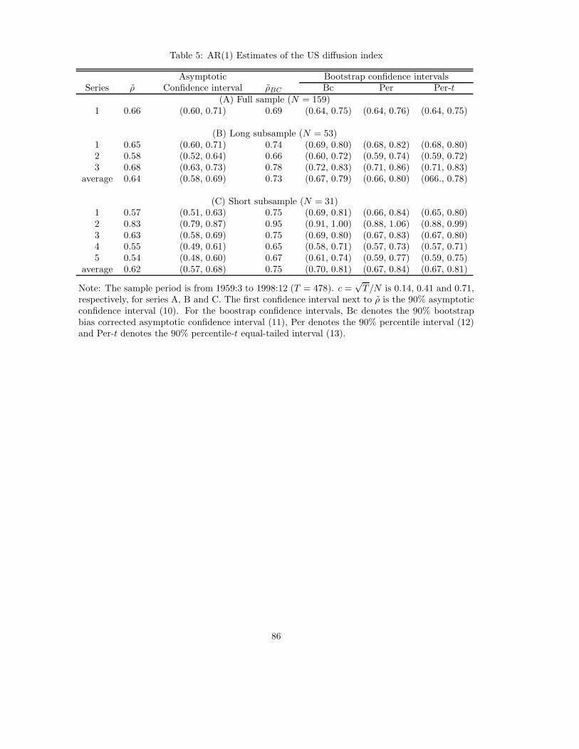
Table 5: AR(1) Estimates of the US diffusion index
Asymptotic Bootstrap confidence intervalsSeries ρ Confidence interval ρBC Bc Per Per-t
(A) Full sample (N = 159)1 0.66 (0.60, 0.71) 0.69 (0.64, 0.75) (0.64, 0.76) (0.64, 0.75)
(B) Long subsample (N = 53)1 0.65 (0.60, 0.71) 0.74 (0.69, 0.80) (0.68, 0.82) (0.68, 0.80)2 0.58 (0.52, 0.64) 0.66 (0.60, 0.72) (0.59, 0.74) (0.59, 0.72)3 0.68 (0.63, 0.73) 0.78 (0.72, 0.83) (0.71, 0.86) (0.71, 0.83)
average 0.64 (0.58, 0.69) 0.73 (0.67, 0.79) (0.66, 0.80) (066., 0.78)
(C) Short subsample (N = 31)1 0.57 (0.51, 0.63) 0.75 (0.69, 0.81) (0.66, 0.84) (0.65, 0.80)2 0.83 (0.79, 0.87) 0.95 (0.91, 1.00) (0.88, 1.06) (0.88, 0.99)3 0.63 (0.58, 0.69) 0.75 (0.69, 0.80) (0.67, 0.83) (0.67, 0.80)4 0.55 (0.49, 0.61) 0.65 (0.58, 0.71) (0.57, 0.73) (0.57, 0.71)5 0.54 (0.48, 0.60) 0.67 (0.61, 0.74) (0.59, 0.77) (0.59, 0.75)
average 0.62 (0.57, 0.68) 0.75 (0.70, 0.81) (0.67, 0.84) (0.67, 0.81)
Note: The sample period is from 1959:3 to 1998:12 (T = 478). c =√
T/N is 0.14, 0.41 and 0.71,respectively, for series A, B and C. The first confidence interval next to ρ is the 90% asymptoticconfidence interval (10). For the boostrap confidence intervals, Bc denotes the 90% bootstrapbias corrected asymptotic confidence interval (11), Per denotes the 90% percentile interval (12)and Per-t denotes the 90% percentile-t equal-tailed interval (13).
86
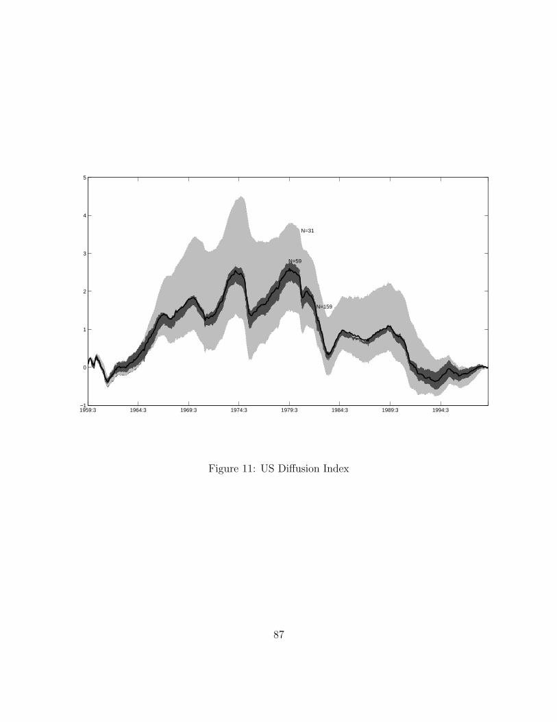
1959:3 1964:3 1969:3 1974:3 1979:3 1984:3 1989:3 1994:3−1
0
1
2
3
4
5
N=159
N=31
N=59
Figure 11: US Diffusion Index
87

CHAPTER III
INFORMATION HETEROGENEITY, HOUSING DYNAMICS AND THE BUSINESSCYCLE
Introduction
The recent �nancial crisis that started in the U.S. in December 2007 has demon-
strated the importance of the housing sector in macroeconomic modeling. In response to
the recession, a growing literature has tried to incorporate the housing sector into standard
macroeconomic models to explain stylized facts in the housing market and the business
cycle.1 However, there are two facts that existing quantitative macroeconomic models have
di¢ culty explaining: house prices are highly volatile and closely correlated with the busi-
ness cycle, which is at odds with the evidence that rental prices are relatively stable and
almost uncorrelated with the business cycle; and residential investment leads the business
cycle while nonresidential investment moves contemporaneously with the business cycle.
The main goal of this paper is to present an alternative model to quantitatively
explain these two facts. To incorporate the housing sector into the standard dynamic sto-
chastic general equilibrium (DSGE) model, one usually assumes that �rms need a collateral
asset to secure their external �nancing as in Kiyotaki and Moore (1997), and speci�es the
collateral asset as houses, such as Iacoviello (2005), and Liu, Wang, and Zha (2011) et al.
These types of models succeed in explaining either the close correlation between house prices
and nonresidential investment or the close correlation between house prices and consump-
tion, but fails in explaining the contrast between the high volatility of house prices and the
low volatility of rental prices. Figure 12 illustrates the cyclical components of house prices
and rental prices with the business cycle for the United States from 1975Q1 to 2010Q32
1Iacoviello (2010) is a recent survey. A inexhaustive reading list should include Iacoviello (2005), Davisand Heathcote (2005, 2007), Piazzesi and Schneider (2009), Iacoviello and Neri (2010), Liu, Wang, and Zha(2011), Sterk (2010), Burnside, Eichenbaum, and Rebelo (2011), Caplin and Leahy (2011), Chaney, Sraer,and Thesmar (2012), Chatterjee and Eyigungor (2011), Favilukis, Ludvigson, and Nieuwerburgh (2011),Mian and Su� (2011), Kiyotaki, Michaelides, and Nikolov (2011), and Rupert and Wasmer (2012).
2In this paper, we collect the data of output, consumption, residential investment, and nonresidentialinvestment from the St. Louis Fed.
88

(all data are log-linearized and �ltered using the Hodrick-Prescott �lter). House prices are
closely correlated with the business cycle and their correlation with U.S. GDP is around
0:52. In contrast, rental prices are almost uncorrelated with the business cycle and their
correlation with U.S. GDP is less than 0:06. Furthermore, house prices are much more
volatile than output and their standard deviation is around 1:55 times of the standard devi-
ation of output. However, rental prices are much less volatile and their standard deviation
is only 0.46 times of the standard deviation of output. To explain the di¤erence between
the volatility of house prices and the volatility of rental prices, in addition to incorporat-
ing �nancial frictions as in Liu, Wang, and Zha (2011), we further incorporate information
frictions into the standard DSGE model, and demonstrate that information heterogeneity
plays a key role in quantitative macroeconomic analysis of housing dynamics.
In the standard DSGE model with �nancial frictions, houses can be viewed as
assets (see equation (20) in Liu, Wang, and Zha (2011)). If we de�ne the rental prices as
the marginal rate of substitution (MRS) between housing consumption and goods consump-
tion, the asset pricing theory implies that house prices are determined by the discounted
sum of future rents. With consumption smoothing, the model predicts that the volatility of
house prices is much lower than the volatility of output (see Liu, Wang, and Zha (2011) for
a detailed discussion). However, if households have heterogeneous information about the
future average MRS between housing consumption and goods consumption, house prices
will also be determined by households�expectations of other households�expectations of the
future average MRS, households�expectations of other households�expectations of other
households�expectations of the future average MRS, and so on. Therefore, higher-order ex-
pectations of the future average MRS play a potential role in determining the �uctuations
of house prices. Our calibration exercise shows that information heterogeneity increases the
relative volatility of house prices to output by more than 50% and explain the disconnect
between house prices and the discounted sum of future rents compared with the full infor-
mation case. However, our model still has a di¢ culty in predicting house prices having a
higher volatility than output.
We assume households�information sets di¤er in two respects. First, households
have dispersed information of the total factor productivity (TFP). Second, households have
89
idiosyncratic information of the aggregate preferences on houses. When house prices rise,
households are confused by whether this rise is driven by an improvement in TFP or an
increase in the aggregate demand. Because of rational confusion, an improvement in TFP
has an ampli�ed e¤ect on house prices3. Thus, information heterogeneity generates a higher
volatility of house prices, and breaks down the close correlation between house prices and
rental prices.
The other fact which standard macroeconomic models have di¢ culty in explain-
ing is the lead-lag relationship between residential investment and nonresidential investment
over the business cycle. Figure 13 displays the normalized cyclical components of residential
and nonresidential investment over the business cycle for the United States from 1975Q1 to
2010Q3, and shows that residential investment leads the business cycle while nonresidential
investment moves contemporaneously with the business cycle. The reason why standard
real macroeconomic models have di¢ culty in explaining the lead-lag relationship is because
nonresidential capital produces market consumption and investment goods, whereas resi-
dential capital produces only home consumption goods (e.g. Fisher, 2007). The asymmetry
in how many goods to substitute away from residential capital provides a strong incentive to
substitute away from residential capital toward nonresidential capital after a productivity
shock. In our model, with incomplete information �rms cannot fully observe the true TFP
shocks, so the model generates a dampened response of nonresidential investment to TFP
shocks. On the other side, since the ampli�ed response of house prices mainly comes from
the rising demand of real estate from households, the response of residential investment
to TFP shocks is dampened, but to a smaller degree. In total, the correlation between
lead residential investment and nonresidential investment increases, as does the correlation
between lead residential investment and output. Our calibration shows that the correlation
between lead residential investment and nonresidential investment increases from a negative
value to a large positive value.
3The idea of rational confusion has long existed in the noisy rational expectation literature. For example,Bulow and Klemperer (1994) use this idea to explain the worldwide stock market crash of 1987. Bacchettaand van Wincoop (2006) claim that such rational confusion plays a key role in explaining the exchange ratedisconnect puzzle and matching the evidence on micro trading activities.
90
The paper is related to several strands of the literature. First, it is related to the
literature incorporating �nancial frictions into models of business cycles (see Gertler and
Kiyotaki, 2010, for a survey). Within this strand, there is a large body of work that speci�es
houses as a collateral asset, and investigates frictions in the house market a¤ecting the
business cycle1. For example, Iacoviello (2005) introduces collateral constraints tied to home
values into a standard monetary business cycle model and shows that houses contribute to
the ampli�cation and propagation of demand shocks. In terms of the labor market, Rupert
and Wesmer (2012) incorporate frictions in housing mobility into a standard searching and
matching model to investigate the di¤erence of unemployment rates between the U.S. and
Europe. Sterk (2011) studies the e¤ect of the housing bust in 2007 on the unemployment rate
of the recent �nancial crisis. However, these models either do not consider the disconnect
between house prices and rental prices or have di¢ culty in explaining it. Liu, Wang, and Zha
(2011) estimate a real business cycle model with land as a collateral asset in �rms�credit
constraints, and claim that a shock originated from households�preferences on houses is
important in determining land prices and the business cycle. In their model, the housing
demand shock explains more than 90% of the observed �uctuations of land prices, and other
shocks make almost no contributions, which seems counterintuitive4.
In this paper, we investigate information frictions in explaining the high volatility
of house prices. Trading with information frictions in the housing market has been consid-
ered in the literature for a long time (see Himmelberg, Mayer, and Sinar, 2005, for a survey).
For recent evidence, Piazzesi and Schneider (2009) propose a search model with transac-
tion costs and show that a small portion of momentum trades generates a high volatility
of house prices. Burnside, Eichenbaum, and Rebelo (2011) develop a model with hetero-
geneous expectations and show that changes in expectations can generate the boom-bust
cycles in the housing market. However, these models are not in a micro-founded general
equilibrium framework, and therefore are not suitable for a quantitative analysis of the
interaction of information frictions and the housing dynamics over the business cycle. To
the best of my knowledge, this paper is the �rst to introduce imperfect information into
4The other shocks include a patience shock, permanent and transitory shocks to neutral technology,permanent and transitory shocks to biased technology, a labor supply shock, and a collateral shock.
91

the standard DSGE model with a housing sector, and shows information heterogeneity has
the potential to explain the aforementioned puzzles in both the housing market and the
macroeconomy. Our paper is also the �rst one to introduce information frictions to explain
the lead-lag relationship between residential investment and business investment. Previous
literature investigating the lead-lag relationship includes Benhabib, Rogerson, and Wright
(1991), Greenwood and Hercowitz (1991), Chang (2000), Gomme, Kydland, and Rupert
(2001) Davis and Heathcote (2005), Fisher (2007), et al.
Finally, this paper also contributes to the growing interests in investigating im-
perfect information in macroeconomics5. In their seminal work, Phelps (1970) and Lucas
(1972) demonstrate that the dispersion of information can help nominal shocks generate
�uctuations in real variables. Recently, Morris and Shin (2002) investigate strategic in-
teractions in a global game framework; Mankiw and Reis (2002) consider the case that
agents update their information sets sporadically; and Sims (2003) formalizes the idea of
information frictions by assuming limited capacity for processing information. Our work
is more closely related with La�O (2010), which also studies the interaction of information
frictions with �nancial frictions. However, our work di¤ers from La�O�s work in three as-
pects. First, our work directly investigates the information frictions in the housing market
and the spillover e¤ects from the housing market to the business cycle. Second, we build our
model in a dynamic stochastic general equilibrium framework and thus can quantitatively
evaluate the contribution of information heterogeneity to both the housing market and the
business cycle. Finally, La�O�s work focuses on how the interactions of �nancial frictions
and information frictions a¤ect noise shocks as an independent source of the business cycle
�uctuations.
The remainder of the paper is organized as follows. Section 2 provides empirical
evidence about the two facts in the housing market and the business cycle. Section 3
introduces the model with both �nancial frictions and information frictions. Section 4
discusses the implications of our model regarding house prices, residential investment, and
5Mankiw and Reis (2010) provide a recent survey. An inexhaustive list includes Phelps (1970), Lucas(1972), Townsend (1983), Mankiw and Reis (2002), Morris and Shin (2002), Sims (2003), Woodford (2003),Bacchetta and van Wincoop (2006), Nimark (2008), Lorenzoni (2009), Machowiak and Wiederholt (2009),Angeletos and La�O (2010), Graham and Wright (2010), and Guo and Shintani (2011), Crucini, Shintani,and Tsuruga (2010, 2012).
92
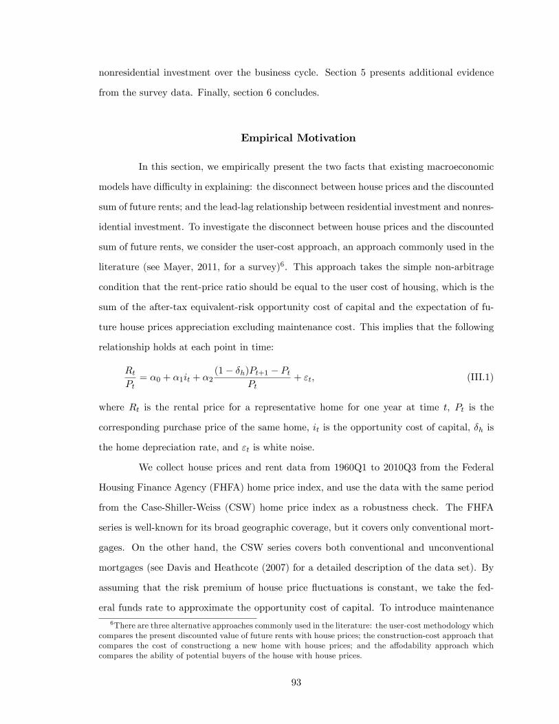
nonresidential investment over the business cycle. Section 5 presents additional evidence
from the survey data. Finally, section 6 concludes.
Empirical Motivation
In this section, we empirically present the two facts that existing macroeconomic
models have di¢ culty in explaining: the disconnect between house prices and the discounted
sum of future rents; and the lead-lag relationship between residential investment and nonres-
idential investment. To investigate the disconnect between house prices and the discounted
sum of future rents, we consider the user-cost approach, an approach commonly used in the
literature (see Mayer, 2011, for a survey)6. This approach takes the simple non-arbitrage
condition that the rent-price ratio should be equal to the user cost of housing, which is the
sum of the after-tax equivalent-risk opportunity cost of capital and the expectation of fu-
ture house prices appreciation excluding maintenance cost. This implies that the following
relationship holds at each point in time:
RtPt= �0 + �1it + �2
(1� �h)Pt+1 � PtPt
+ "t; (III.1)
where Rt is the rental price for a representative home for one year at time t, Pt is the
corresponding purchase price of the same home, it is the opportunity cost of capital, �h is
the home depreciation rate, and "t is white noise.
We collect house prices and rent data from 1960Q1 to 2010Q3 from the Federal
Housing Finance Agency (FHFA) home price index, and use the data with the same period
from the Case-Shiller-Weiss (CSW) home price index as a robustness check. The FHFA
series is well-known for its broad geographic coverage, but it covers only conventional mort-
gages. On the other hand, the CSW series covers both conventional and unconventional
mortgages (see Davis and Heathcote (2007) for a detailed description of the data set). By
assuming that the risk premium of house price �uctuations is constant, we take the fed-
eral funds rate to approximate the opportunity cost of capital. To introduce maintenance6There are three alternative approaches commonly used in the literature: the user-cost methodology which
compares the present discounted value of future rents with house prices; the construction-cost approach thatcompares the cost of constructiong a new home with house prices; and the a¤odability approach whichcompares the ability of potential buyers of the house with house prices.
93

costs, we assume that houses depreciate at a constant rate �h = 0:01 as in Iacoviello and
Neri (2010). Table 6 presents the regression results of equation (III.1). The results show
that appreciation in house prices has almost no explanatory power in the �uctuations of
the rent-price ratio. One percent increases in house prices predict around 0:09 increases in
rent-price ratio for the FHFA series, and around 0:02 increases for the CSW series. The null
hypothesis �2 = 1 is rejected at any signi�cance level for both of the two data sets. Thus,
the regression results con�rm the disconnect between house prices and the discounted sum
of future rents.
The second fact that we want to investigate is the lead-lag relationship between
residential investment and nonresidential investment over the business cycle. The litera-
ture in home production has demonstrated that residential investment leads the business
cycle and nonresidential investment lags the business cycle for the U.S. economy (see Davis,
2010, for a survey). In sharp contrast, Kydland, Rupert, and �ustek (2012) empirically show
that the lead-lag relationship in the developed countries only holds for the two Western-
Hemishpere countries: USA and Canada, and in other developed economies there is no
such a clear feature of the lead-lag relationship between either residential investment or
nonresidential investment and the business cycle. We reconsider the fact and calculate the
correlations among the lead (lag) residential investment, the lead (lag) business investment,
and the lead (lag) output for the following countries and periods: Austria (1988Q1-2012Q2),
Finland (1975Q1-2012Q2), France (1978Q1-2012Q2), Netherlands (1988Q1-2012Q2), the
U.K. (1970Q1-2012Q2), the EU (1988Q1-2012Q2), Australia (1959Q3-2012Q2), Canada
(1981Q1-2012Q2), and the U.S. (1960Q1-2012Q2)7. All the data are logged and Hodrick-
Prescott �ltered. In Table 7, our main results con�rm the leading (lagged) role of residential
(nonresidential) investment over the business cycle in the U.S. and Canada. In other devel-
oped countries, there is no clear order among the second moments except Finland, which
also shares this feature to some extent. One interesting thing in our calculation is that if
we aggregate the �ve countries in the Europe together, the aggregate will also somewhat
perform like the U.S. and Canada.
7The EU is aggregated by the �ve following countries: Austria, Finland, France, Netherlands, and theU.K.. We collect the data for the European countries from the Eurostat, for Canada from the OECD, forAustralia from Australian Bureau of Statistics, and for the U.S. from the St. Louis Fed.
94
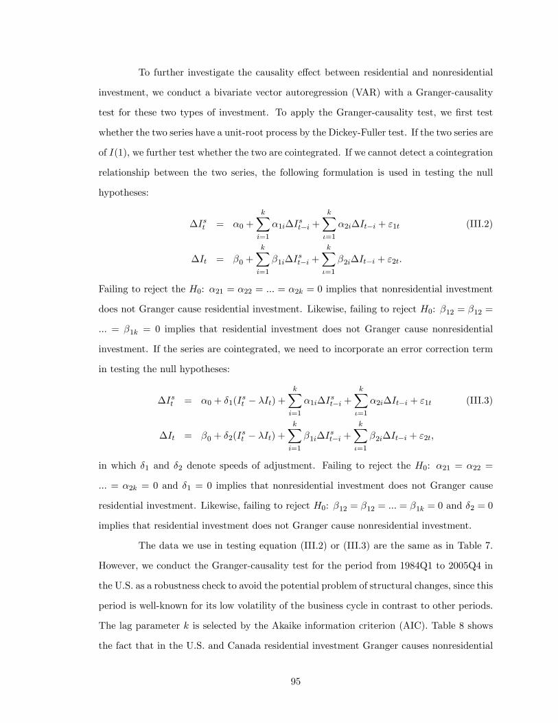
To further investigate the causality e¤ect between residential and nonresidential
investment, we conduct a bivariate vector autoregression (VAR) with a Granger-causality
test for these two types of investment. To apply the Granger-causality test, we �rst test
whether the two series have a unit-root process by the Dickey-Fuller test. If the two series are
of I(1), we further test whether the two are cointegrated. If we cannot detect a cointegration
relationship between the two series, the following formulation is used in testing the null
hypotheses:
�Ist = �0 +
kXi=1
�1i�Ist�i +
kX�=1
�2i�It�i + "1t (III.2)
�It = �0 +kXi=1
�1i�Ist�i +
kX�=1
�2i�It�i + "2t:
Failing to reject the H0: �21 = �22 = ::: = �2k = 0 implies that nonresidential investment
does not Granger cause residential investment. Likewise, failing to reject H0: �12 = �12 =
::: = �1k = 0 implies that residential investment does not Granger cause nonresidential
investment. If the series are cointegrated, we need to incorporate an error correction term
in testing the null hypotheses:
�Ist = �0 + �1(Ist � �It) +
kXi=1
�1i�Ist�i +
kX�=1
�2i�It�i + "1t (III.3)
�It = �0 + �2(Ist � �It) +
kXi=1
�1i�Ist�i +
kX�=1
�2i�It�i + "2t;
in which �1 and �2 denote speeds of adjustment. Failing to reject the H0: �21 = �22 =
::: = �2k = 0 and �1 = 0 implies that nonresidential investment does not Granger cause
residential investment. Likewise, failing to reject H0: �12 = �12 = ::: = �1k = 0 and �2 = 0
implies that residential investment does not Granger cause nonresidential investment.
The data we use in testing equation (III.2) or (III.3) are the same as in Table 7.
However, we conduct the Granger-causality test for the period from 1984Q1 to 2005Q4 in
the U.S. as a robustness check to avoid the potential problem of structural changes, since this
period is well-known for its low volatility of the business cycle in contrast to other periods.
The lag parameter k is selected by the Akaike information criterion (AIC). Table 8 shows
the fact that in the U.S. and Canada residential investment Granger causes nonresidential
95

investment and nonresidential investment does not Granger cause residential investment.
This fact is very clear in Canada, but in the U.S., we can reject the null hypothesis that
residential investment does not Granger cause nonresidential investment at any signi�cance
level, whereas we cannot reject the null hypothesis that nonresidential investment does
not Granger cause residential investment for the period from 1984Q1 to 2005Q4 at 5%
signi�cance level, and for the period from 1960Q1 to 2010Q3 at 1% signi�cance level. In
other developed countries, there is no such feature similar as in the U.S. and Canada,
except in Australia and the U.K. In contrast to the lead-lag relationship that the European
aggregate shares with the U.S. and Canada, we cannot see such a similarity for the Granger
causality of the two types of investment between the two regions.
The Basic Model
To quantitatively explain the two facts in a dynamic general equilibrium frame-
work, we build our model in the style of Liu, Wang, and Zha (2011) with real estate
production and information heterogeneity. The model in Liu, Wang, and Zha (2011) is
a variant of standard real business cycle models that include a feature of credit frictions
(Kiyotaki and Moore, 1997). We add a real estate production sector into the model, and
assume agents are endowed with heterogeneous information instead of perfect information.
Following Iacoviello (2005), Iacoviello and Neri (2010), Kiyotaki, Michaelides, and Nikolov
(2011), and Liu, Wang and Zha (2011), we assume two types of agents in the economy:
a representative impatient entrepreneur and a continuum of patient households. The rep-
resentative entrepreneur owns two types of �rms: a continuum of residential �rms and a
continuum of nonresidential �rms. The whole economy is segmented geographically and
endowed with a continuum of islands. Each island i 2 [0; 1] contains one residential �rm,
one nonresidential �rm, and one household. The residential �rm hires labors from the
household, and accumulates residential structures to build houses. The nonresidential �rm
also hires labor from the household, accumulates nonresidential capital, and combines with
real estate input to produce �nal goods. The household provides labor services, saves for
next period, and consumes �nal goods and housing services. The �nal goods can be used to
96
�nance residential investment and nonresidential investment, whereas real estate can only
be used for residence.
Entrepreneurs
The representative entrepreneur owns a continuum of residential �rms and a con-
tinuum of nonresidential �rms. On each island resides one residential �rm and one nonresi-
dential �rm. The residential �rm and the nonresidential �rm maximize their expected pro�ts
and return the pro�ts to the entrepreneur. The nonresidential �rm i takes a Cobb-Douglas
constant-to-scale technology that uses labor, capital, and housing as input, according to
Yit = K�kit (AtAitN
0kit )
vkH01��k�vkit ;
where Yit is the output, At is the aggregate technology level, Ait is the �rm-speci�c tech-
nology level, Kit is capital produced at the end of last period, H0it is the real estate input,
and N0kit is the labor input in the nonresidential market. �k and 1 � �k � vk measure
output share of capital and real estate respectively. The residential �rm i also takes a
Cobb-Douglas constant-to-scale technology that uses labor, residential structures, and land
as input, according to
H0it = S
�hit (AtAitN
0hit )
vhL1��h�vhit ;
where H0it is newly built housing, Sit are residential structures, Lit is the land endowment,
and N0hit is the labor input in the residential market. �h and 1��h�vh measure output share
of residential structures and land respectively. The representative entrepreneur borrows Bit
from household i in the asset market, invests Iit in the nonresidential capital market and
Isit in the residential structure market, produces consumption �nal goods by purchasing real
estate input �(Hit) and hiring workers Nkit, constructs houses by using the land endowment
Lit, the labor input Nhit, and the residential structure Sit, and consumes C
0t to maximize its
97
expected utility according to
maxE
1Xt=0
�0tC
01� t
1�
s:t: C0t +
ZI[(N
0kit +N
0hit )Wit �
�itBit+1Rit
+ Pt(H0it � (1� �h)H
0it�1) + Iit + I
sit �
K�kit (AitAtN
0kit )
vkH01��k�vkit � PtS�hit (AitAtN
0hit )
vhL1��h�vhit +Bit]di = 0
where �0is the discount factor of the entrepreneur, measures the relative risk aversion,Wit
is the wage that the entrepreneur pays for workers from the household i, �it is the island-
speci�c bond-holding shock, Rit is the island-speci�c interest rate, �h is the discount factor
of houses, and Pt is house prices. The island-speci�c bond-holding shock �it serves one and
only one role, to slow down the learning of agents in island i from the bond market. To
replace the assumption of the island-speci�c bond-holding shock, one can introduce another
aggregate shock, such as a patience shock to the entrepreneur, to serve a similar role. For
simplicity, we do not consider adding another aggregate shock. As in Kiyotaki and Moore
(1997), we assume the entrepreneur needs collateral to secure its borrowings
Bit+1 � mEit(Pt+1H0it); (III.4)
where m indicates that if borrowers repudiate their debt obligations, lenders can liqui-
date the borrowers� real estate assets but have to pay a proportional transaction cost
(1�m)Pt+1Hit. Allowing capital as an additional collateral asset will amplify the e¤ect of
credit constraints since the entrepreneur will be more leveraged. We will discuss this later
as a robustness check. Nonresidential capital accumulation follows the law of motion
Kit+1 = (1� �k)Kit +�1(IitKit
)Kit;
and similarly, residential structure accumulation follows the law of motion
Sit+1 = (1� �s)Sit +�2(IsitSit)Sit;
where �k and �s are the discount factors of nonresidential capital and of residential structures
respectively, and �1(�) and �2(�) denote the adjustment cost functions of nonresidential
capital and of residential structures respectively.
98

Households
We assume one household resides on each island i. The household i consumes
the �nal goods, utilitzes the housing services, and provides labor services to the residential
�rm and the nonresidential �rm. The household maximizes its expected discounted sum of
utility conditional on its own information set it by
maxEi
1Xt=0
�t[lnCit + �0�t�it lnHit � Nit];
where Cit is goods consumption, Hit is the housing consumption, Nit is the labor services
provided by the household, � is the discount factor, �t and �it denote the aggregate and the
idiosyncratic housing preference shocks respectively, and �0 and are constant parameters.
We assume households�discount factor � > �0, which indicates that households are more
patient than the entrepreneur and inclined to save. The household i�s budget constraint is
given by
Cit + Pt(Hit � (1� �h)Hit�1) +Bit+1Rit
�WitNit �Bit = 0:
Market Clearing
The economy has four markets in total: goods, labor, bond and housing. To clear
the goods market, we have
C0t +
ZI[Cit + Iit + I
sit]di =
ZIYitdi:
We assume labor is immobile across islands, so in island i we have
Nit = N 0kit +N
0hit :
To clear the bond market, we have
Bit +B0it = 0:
99
Finally, to clear the housing market, we haveZI[Hit +H
0it � (1� �h)(Hit�1 +H 0
it�1)]di =
ZIH0itdi:
Shocks
Our model includes two aggregate shocks and three idiosyncratic shocks. The
aggregate shocks follow AR(1) processes in logs,
logAt = �a logAt�1 + uat
log�t = �� log�t�1 + u�t ;
where uat � N(1; �2a), and u�t � N(1; �2�). The idiosyncratic shocks also follow the AR(1)
processes in logs
logAit = �ai logAit�1 + uait
log�it = ��i log�it�1 + u�it
log �it = ��i log �it�1 + u�it;
where uait � N(1; �2ai), u�it � N(1; �2�i), and u
�it � N(1; �2�i). We also assume the law of
large numbers applies for the distribution of all the three types of idiosyncratic shocks, as
is common in the literature.
The Information Structure and the Equilibrium
At each period t, the representative entrepreneur has full information. However,
the �nal goods �rm i, the real estate �rm i, and the household i can only obtain information
from their market activities: idiosyncratic preferences series on houses f�t�s�it�sg1s=0, wage
series fWit�sg1s=0, interest rate series fRit�sg1s=0, and house prices series fPt�sg1s=0. The
information set for agents in island i is denoted as
it = ff�t�s�it�sg1s=0; fWt�sg1s=0; fRit�sg1s=0; fPt�sg1s=0g:
100
We assume the parameters and the model structure are common knowledge, which indicates
our model is in line with the framework of noisy rational expectation models.
The equilibrium is de�ned as follows:
1. Given prices and information restrictions, the allocations solve the utility maximiza-
tion problem of the entrepreneur and of the household i and the pro�t maximization
problem of the �nal goods �rm i and the real estate �rm i.
2. All markets clear, and fPt�s; Rit�s;Wit�sg1s=0 are the market clearing house prices,
interest rates of bonds, and wages, respectively.
Economic Implications
In our model, we assume residential �rms, nonresidential �rms, and households
do not have full information about the economic fundamentals and di¤er in their informa-
tion sets for di¤erent islands. Instead of an ad hoc assumption of perfect information, we
assume agents can only extract information about the true economic fundamentals from
their idiosyncratic market activities. With information heterogeneity, agents make their
decisions based on their forecasts of not just true economic fundamentals but also forecasts
of other agents�actions, forecasts of other agents�forecasts of other agents�actions, etc. In
this section, we show that higher-order beliefs play a potential explanatory role in the two
facts: the disconnect between house prices and rental prices, and the lead-lag relationship
between residential investment and nonresidential investment over the business cycle.
Solving a dynamic general model with dispersed information requires dealing with
the well-known "in�nite regress" problem (Townsend, 1983), since higher-order beliefs are
crucial for the decisions of agents and depend on the entire history of shocks. The literature
has solved this type of model by either truncating the dependence of equilibrium actions on
higher order beliefs (Nimark, 2008) or by assuming private information is revealed after an
ad hoc period T (Lorenzoni, 2009). We take the second approach, and assume that after T =
30 periods all of the shocks are observed by agents across islands. The choice of T is based
101
on two considerations: saving computational time and not a¤ecting the results signi�cantly
if the value of T is increased. We assume all the shocks are relatively small in magnitude,
so the inequality in (III.4) is always binding. Without the problem of occasional binding,
one can solve the model by log-linearizing around the steady state. After log-linearization,
we solve the linear equations by combining Sims�s (2001) method and the guess-veri�cation
approach. In the model economy, agents on island i are integrated into two aggregate
markets: the �nal goods market and the housing market. Therefore, decisions of agents
are a¤ected by two aggregate variables: consumption of the representative entrepreneur C0t
and house prices Pt. In the �rst step, we guess the aggregate variables, C0t and Pt, to be
linear functions of aggregate shocks; in the second step, we plug these two variables into the
equations and solve the equations using Sims�s (2001) method; in the third step, we update
expectation operators of agents on island i by their information set it; �nally, we verify
the guess of linear functions of C0t and Pt by minimizing their distance with the updated
variables C0t and Pt. The appendix provides a detailed description of the method.
To calibrate the model, we choose the parameters commonly used in the literature
(e.g. Iacoviello and Neri, 2010). � and �0are set to 0:9925 and 0:97 respectively. Relative
risk aversion, , is set to 2. The housing preference parameter �0 is set to 0:1 and the
disutility on labor is set to 1. The entrepreneurial "loan-to-value ratio" m is set to 0:89
to match the empirical debt to GDP ratio in the U.S. data. The nonresidential capital
share in the output production function is set to �k = 0:63, and the house share is set to
1��k�vk = 0:05. For the real estate production function, the share of residential structures
is set to �h = 0:1, and the share of land is set to 1��h� vh = 0:1. The discount factors for
houses, residential structures, and nonresidential capital are set to �h = 0:01, �s = 0:25, and
�k = 0:03 respectively. These three discount factors, combined with the capital share in the
goods production function and real estate production function, imply that nonresidential
investment accounts for around 30% of the total output, residential investment accounts for
about 6% of the total output, and the value of house stocks is about 1:80 time the total
output. The solution method does not require us to specify the functional form of �1 and
�2, but needs us to set the values of �1, �01, �001, �2, �
02, and �
002 in the steady state. We
choose �1( IK ) = �k, �01(IK ) = 1, �2( I
s
S ) = �s, and �01(Is
S ) = 1, so that the model with
102
adjustment costs has the same steady state as the model without adjustment costs. We
set the second-order derivative of the adjustment cost function of residential investment
�002(Is
S ) = �2:5, the same as that of nonresidential investment �001(
IK ) = �2:5. The later is
chosen as in Christiano, Eichenbaum, and Evans (2005)8.
There are two aggregate and three idiosyncratic AR(1) shock processes in total.
Two parameters are crucial for the AR(1) processes: the persistence and the variance of the
shocks. The persistence and the variance of the shocks a¤ect the response of business cycle
variables in two di¤erent ways: �rst, the shocks to the model are directly a¤ected; second,
the precision of agents�information and agents�information updating process are altered.
For the aggregate technology shock process, we assume a persistent shock process and set
�a = 0:95 as in Fisher (2005). Similarly, the autocorrelation in the aggregate housing
preference shock is assumed to be �� = 0:95. We choose �2a = 0:009842 to match the
volatility of output, and �2� =1102�2a to weaken the e¤ect of housing preference shocks and
focus on technology shocks as a main driving force of the business cycle �uctuations9. Since
our interest is in the role of information heterogeneity in matching aggregate business cycle
variables, we choose the persistence and the variance of idiosyncratic shocks to maximize
the e¤ect of information heterogeneity on house prices, and ignore the empirical micro-level
cross-sectional facts. For the idiosyncratic bond-speci�c shock processes, we set ��i = 0
and �2�i = 1 for one and only one reason: to screen the information contained by the
real interest rate. For the idiosyncratic technology shock and the idiosyncratic housing
preference shock, we set �ai = 0:001, ��i = 0:001, �2ai = 1002�2a and �2�i = 1002�2a. The
high magnitude of idiosyncratic shocks implies that agents extract information mainly from
house prices instead of idiosyncratic variables, such as island-speci�c wages and island-
speci�c technology shocks. This assumption of a large magnitude of idiosyncratic shocks
relative to aggregate shocks has been used in the literature (Mackowiak and Wiederholt,
2009).
8In the literature, one usually pins down the parameters �001 (IS) and �001 (
Is
S) by matching the volatility of
nonresidential investment and residential investment in the data, Unfortunately, our solving procedure can�nd a convergence point only for certain ranges of parameters values. Of course, this is left for future work.
9In our model, a low magnitude of the housing preference shocks is enough to confuse the rational agents.Nimark (2008) makes a similar assumption that the variance of the transitory labor supply shock is 1
100of
other aggregate shocks, such as the technology shock.
103

To evaluate the model�s performance, we turn on all the shocks and simulate the
model 1; 000 times with 142 periods in each simulation. The simulated data are then �ltered
with the Hodrick-Prescott �lter. The average second moments of all the simulations and
their empirical counterparts are reported in Table 9. Our model con�rms the main argu-
ments in Liu, Wang, and Zha (2011) that collateral constraints in nonresidential investment
play a key role in explaining the close correlation between house prices and other business
cycle variables. All of the correlations between house prices and other business cycle vari-
ables for the simulated data are well above their empirical counterparts. In comparison
with the model with full information, two facts stand out for the model with heterogeneous
information: �rst, information heterogeneity ampli�es the response of business cycle vari-
ables to technology shocks10; second, the correlation between lead residential investment
and nonresidential investment increases signi�cantly from a negative value to a large posi-
tive value, and exceeds the correlation between lag residential investment and nonresidential
investment. Similarly, the correlation between lead residential investment and output in-
creases signi�cantly from a small positive value to a large positive value, and exceeds the
correlation between lag residential investment and output.
What drives house prices �uctuations?
Table 9 shows that information heterogeneity ampli�es the response of business
cycle variables to technology shocks, especially for house prices, whose standard deviation
in the model with heterogeneous information is about twice the standard deviation in the
model with full information. In contrast, the standard deviation of goods consumption
increases slightly. These two together indicate that our model might be able to explain the
puzzle of the disconnect between house prices and rental prices, since the later is closely
correlated with �nal goods consumption. As discussed in Liu, Wang, and Zha (2011),
the main reason why standard DSGE models with a housing sector cannot predict a high
10Since the standard deviation of housing preference shocks is one-tenth of the standard deviation oftechnology shocks, the role of housing preference shocks in our calibration is limited.
104
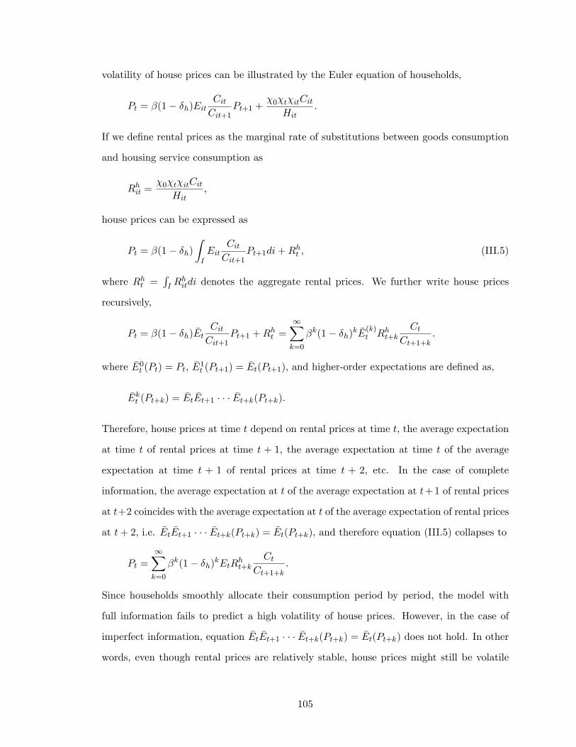
volatility of house prices can be illustrated by the Euler equation of households,
Pt = �(1� �h)EitCitCit+1
Pt+1 +�0�t�itCit
Hit:
If we de�ne rental prices as the marginal rate of substitutions between goods consumption
and housing service consumption as
Rhit =�0�t�itCit
Hit;
house prices can be expressed as
Pt = �(1� �h)ZIEit
CitCit+1
Pt+1di+Rht ; (III.5)
where Rht =RI R
hitdi denotes the aggregate rental prices. We further write house prices
recursively,
Pt = �(1� �h) �EtCitCit+1
Pt+1 +Rht =
1Xk=0
�k(1� �h)k �E(k)t Rht+kCt
Ct+1+k:
where �E0t (Pt) = Pt, �E1t (Pt+1) = �Et(Pt+1), and higher-order expectations are de�ned as,
�Ekt (Pt+k) = �Et �Et+1 � � � �Et+k(Pt+k):
Therefore, house prices at time t depend on rental prices at time t, the average expectation
at time t of rental prices at time t + 1, the average expectation at time t of the average
expectation at time t + 1 of rental prices at time t + 2, etc. In the case of complete
information, the average expectation at t of the average expectation at t+1 of rental prices
at t+2 coincides with the average expectation at t of the average expectation of rental prices
at t+ 2, i.e. �Et �Et+1 � � � �Et+k(Pt+k) = �Et(Pt+k), and therefore equation (III.5) collapses to
Pt =1Xk=0
�k(1� �h)kEtRht+kCt
Ct+1+k:
Since households smoothly allocate their consumption period by period, the model with
full information fails to predict a high volatility of house prices. However, in the case of
imperfect information, equation �Et �Et+1 � � � �Et+k(Pt+k) = �Et(Pt+k) does not hold. In other
words, even though rental prices are relatively stable, house prices might still be volatile
105

since house prices are also determined by higher-order expectations of future rental prices.
Figure 14 displays the response of house prices to one positive standard deviation of tech-
nology shocks in the models with full information and in the model with heterogeneous
information. Information heterogeneity initially dampens the technology shocks, but am-
pli�es and propagates the technology shocks after three quarters. Unfortunately, our model
still fails to generate a higher volatility of house prices than output. To illustrate how in-
formation heterogeneity a¤ects house prices, we plot the average expectation of next-period
house prices for both the full information case and the heterogeneous information case in
Figure 15, since equation (III.5) shows that it is crucial in determining house prices in this
period. The �gure displays that the model with heterogeneous information is accompanied
by higher average expectations of house prices.
To rigorously prove that information heterogeneity can explain the disconnect
between house prices and rental prices, we test the user-cost equation as in (III.1) using the
simulated data. The results in Table 10 show that the null hypothesis �2 = 1 cannot be
rejected by the model with full information, but is rejected by the model with heterogeneous
information at 5% signi�cance level. In sum, even though the model with heterogeneous
information cannot predict house prices having a higher volatility than output, it explains
the disconnect puzzle between house prices and rental prices to some level.
Implications for Investment Dynamics
The other prediction of our model is the lead-lag relationship among nonresiden-
tial investment, residential investment, and output. Empirical studies have documented
that residential investment leads the business cycle, but nonresidential investment lags the
business cycle, and the two types of investment are positively correlated with each other
(see Gangopadhyay and Hatchondo, 2009, for a survey). However, standard real business
cycle models with home production predict the opposite and even a large negative value
for the correlation between the contemporaneous residential investment and nonresidential
investment. To match the data, several di¤erent channels have been emphasized in the
literature, including adjustment costs in capital accumulation (Chang, 2000), time-to-build
106
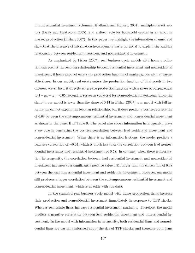
in nonresidential investment (Gomme, Kydland, and Rupert, 2001), multiple-market sec-
tors (Davis and Heathcote, 2005), and a direct role for household capital as an input in
market production (Fisher, 2007). In this paper, we highlight the information channel and
show that the presence of information heterogeneity has a potential to explain the lead-lag
relationship between residential investment and nonresidential investment.
As emphasized by Fisher (2007), real business cycle models with home produc-
tion can predict the lead-lag relationship between residential investment and nonresidential
investment, if home product enters the production function of market goods with a reason-
able share. In our model, real estate enters the production function of �nal goods in two
di¤erent ways: �rst, it directly enters the production function with a share of output equal
to 1��k�vk = 0:05; second, it serves as collateral for nonresidential investment. Since the
share in our model is lower than the share of 0:14 in Fisher (2007), our model with full in-
formation cannot explain the lead-lag relationship, but it does predict a positive correlation
of 0:69 between the contemporaneous residential investment and nonresidential investment
as shown in the panel B of Table 9. The panel also shows information heterogeneity plays
a key role in generating the positive correlation between lead residential investment and
nonresidential investment. When there is no information frictions, the model predicts a
negative correlation of �0:04, which is much less than the correlation between lead nonres-
idential investment and residential investment of 0:58. In contrast, when there is informa-
tion heterogeneity, the correlation between lead residential investment and nonresidential
investment increases to a signi�cantly positive value 0:51, larger than the correlation of 0:38
between the lead nonresidential investment and residential investment. However, our model
still produces a larger correlation between the contemporaneous residential investment and
nonresidential investment, which is at odds with the data.
In the standard real business cycle model with home production, �rms increase
their production and nonresidential investment immediately in response to TFP shocks.
Whereas real estate �rms increase residential investment gradually. Therefore, the model
predicts a negative correlation between lead residential investment and nonresidential in-
vestment. In the model with information heterogeneity, both residential �rms and nonresi-
dential �rms are partially informed about the size of TFP shocks, and therefore both �rms
107
postpone their investment in response to TFP shocks. However, if the ampli�ed house prices
are mainly caused by rising demand from households, real estate �rms will have a stronger
incentive to increase residential investment in response to TFP shocks since the marginal
revenue of real estate production increases. As shown in last subsection, the main reason the
response of house prices is ampli�ed is the breakdown in households�Euler equation (III.5).
In our calibration, we �nd aggregate housing demand from households Ht =RI Hitdi de-
creases by much less in the model with information heterogeneity compared with the model
with full information. Accordingly, residential investment will decrease by much less, and
the correlation between lead residential investment and nonresidential investment increases.
With the delayed response of nonresidential investment, our model predicts a hump-shaped
response of output to one standard deviation of TFP shocks. In the case of imperfect in-
formation, the response of output initially increases at a slow speed and peaks in several
periods. The hump-shaped response of output con�rms the �nding in Nimark (2008) that
imperfect information provides a potential explanation for the contrast between a posi-
tive autocorrelation of output in the data and a negative autocorrelation of output in the
real business cycle theory (Cogley and Nason, 1995). The one-period-lag autocorrelation
increases from �0:10 to 0:04, although not signi�cantly.
Empirical Evidence from Survey Data
A di¢ culty in the literature of imperfect information is that it is hard to provide
empirical evidence to test the model. A prediction of our model is that if we de�ne ex-
pectation errors of real variables as the di¤erence between the average expectation of real
variables and the corresponding realized variables, the expectation errors should be corre-
lated with the business cycle. For instance, the model predicts that the forecast errors of
output are positively correlated with the business cycle in response to TFP shocks with
a correlation of 0:052, since �rms are partially informed about the shocks and agents�ex-
pectations of output tend to underreact. As other variables, such as house prices, are also
positively responded to TFP shocks, if one identi�es an independent shock in the expecta-
tion errors of output, a vector autoregression (VAR) should perform as this shock positively
108
causes other real variables, such house prices, output and investment.
To con�rm this prediction, we run a three-variable VAR with expectation errors
of output, output, and house prices to consider the partial derivatives of output and house
prices at various horizons with respect to shocks in the expectation errors of output. We
compare the results from an empirical VAR to those arising from application of the same
VAR speci�cation to data generated from our model with information heterogeneity. To
measure the average expectation of output, we collect data from the Survey of Professional
Forecasters (SPF). The data cover the period from 1975Q1 to 2010Q3. We take the median
forecasts of real GDP in the coming quarter as the forecast of output. We de�ne the
expectation errors as the percentage deviation of the realized real GDP from the forecast
of real GDP. To see how innovations in the expectation errors a¤ect other variables, we
run the VAR with four lags and the expectation errors ordered �rst. Figure 15 shows the
empirical impulse responses to shocks in expectation errors of output from the trivariate
VAR. The shaded areas represent one-standard-error bias-corrected bootstrap con�dence
bands of Kilian (1998). The �gure shows that one percent increases in agents�expectation
errors are followed by around 0:05 increases in house prices and 0:4 increases in real GDP.
To run a similar trivariate VAR for the model, we collect simulated data with a
length of 142 observations. The average expectations of real variables are directly calculated,
as agents�information sets are clearly de�ned. Similarly, we de�ne the expectation errors
of output as the percent deviation between the average expectation of output and the true
output. The correlation between the expectation errors and output is also a positive value of
0:042. Figure 16 plots the impulse response to one positive standard deviation of shocks in
expectation errors of output from the trivariate VAR for the simulated data. The responses
in the simulated data are as similar as the responses in the empirical data, although they
di¤er in magnitude. A one percent increase in agents� expectation errors is followed by
around a 0:05 percent increase in house prices and a 0:05 percent increase in output. The
main di¤erence between the data sets is that in the simulated data both house prices and
output respond with a hump shape, but in the empiricial data, we do not observe such a
hump.
To check the robustness of the results, we have repeated the VAR exercise using
109

di¤erent variables or di¤erent numbers of variables. For instance, we have replaced the
expectation errors of output by the expectation errors of nonresidential investment, and
replaced output by nonresidential investment. We have also extended the three-variable
VAR to a �ve-variable VAR by adding consumption and nonresidential investment. All of
the regressions report similar qualitative results.
Conclude
The recent standard real business cycle models with �nancial frictions succeed in
explaining the close correlations among house prices, consumption, and investment. How-
ever, the models cannot explain two facts: the disconnect between house prices and rental
prices, and the lead-lag relationship between residential investment and nonresidential in-
vestment. We introduce information heterogeneity into a standard real business cycle model
with real estate production and �nancial frictions. By assuming that agents are rationally
confused about the sources of shocks, the model generates an ampli�ed response of house
prices to technology shocks, which explain the disconnect puzzle. Since the ampli�ed re-
sponse mainly comes from the rising demand of real estate from households, the model
potentially explains the lead-lag relationship between residential investment and nonresi-
dential investment.
There are several directions in which our paper can be improved11. In our model,
although we show information heterogeneity ampli�es the response of house prices to tech-
nology shocks, the volatility of house prices is still much lower compared to the data. One
can introduce monetary shocks into the model and investigate the confusion between real
shocks and nominal shocks, since nominal shocks can also be viewed as pure demand shocks
and therefore may serve a similar role to housing demand shocks in our model. Second, we
could apply the method of minimization of distance between the simulated second moments
and the empirical second moments to pin down parameters for our calibration instead of
choosing ad hoc values. Third, our model extends the standard real business cycle model
in three directions: residential production, �nancial frictions, and information frictions. It11Our solution method can only solve the model using certain ranges of parameters values. Of course, this
is the most central issue to address.
110

is more intuitive to extend the model step by step, so one can clearly discuss how each
extension a¤ects the model. All of these are left for future work.
111

Appendix: Solving a DSGE model with heterogeneous information
The solving procedure consists of four steps in total.
� Step one: shut down all the shocks, solve the model in the steady state, and log-
linearize the model around the steady state. In our model, there are two aggregate
variables which a¤ect agents�decisions: housing prices Pt and the aggregate consump-
tion of the entrepreneur Ct. The later one also determines the stochastic discount
factor. We assume the two aggregate variables are a linear function of aggregate
shocks �t = ffuat�igTi=1; fu�t�igTi=1g, Ct = CC � [uat ; uat�1; :::; uat�T ; u
�t ; u
�t�1; :::; u
�t�T ]
0,
and Pt = PP � [uat ; uat�1; :::; uat�T ; u�t ; u
�t�1; :::; u
�t�T ]
0.
� Step two: replace the goods market clearing condition and the housing market clear-
ing condition by the two above equations of the de�nitions Ct and Pt, and solve the
linear di¤erence equations as a typical rational expectation model.
� Step three: from Step two, we have
Yit = G1Yit�1 +�c +�0z�it;
and then apply an expectation operator to both sides of the above equation conditional
on the information set it
Yit = G1Yit�1 +�c +�0Eitz�it:
To derive Eitz�it, we should �rst keep in mind that the signals sit island i receives are
linear functions of zit, given by,
sit = �zit:
By Kalman �lter updating, we have
Eitzit � E(zitjsit) = ��0(���0)�1sit = ��0(���0)�1�zit:
� Step four: plug the solved individual variables into the goods market clearing con-
dition and the housing market clearing condition, derive the updated C�t and P �t ,
112

and match the distance between (Ct; Pt) and (C�t ; P�t ): If the distance is zero or close
enough to zero, we solve the model. In our calibration, the square root of the distance
is less than 10�3, although we cannot �nd the exact solution.
113
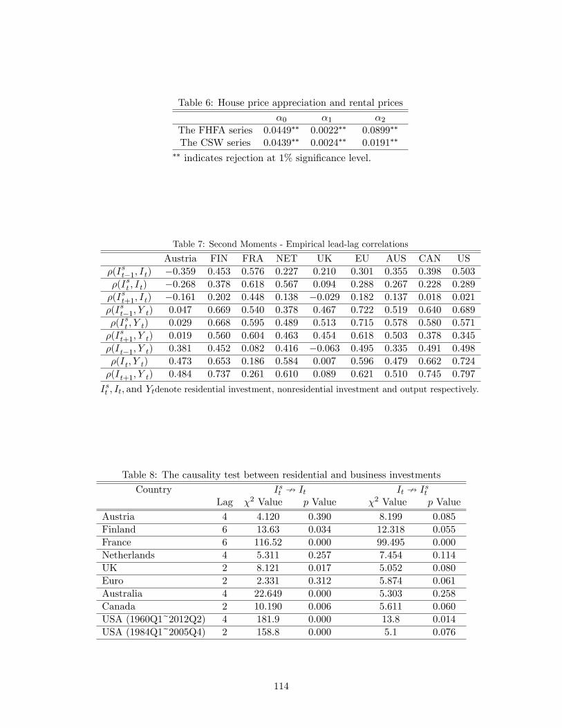
Table 6: House price appreciation and rental prices
�0 �1 �2The FHFA series 0:0449�� 0:0022�� 0:0899��
The CSW series 0:0439�� 0:0024�� 0:0191��
�� indicates rejection at 1% signi�cance level.
Table 7: Second Moments - Empirical lead-lag correlations
Austria FIN FRA NET UK EU AUS CAN US�(Ist�1; It) �0:359 0:453 0:576 0:227 0:210 0:301 0:355 0:398 0:503
�(Ist ; It) �0:268 0:378 0:618 0:567 0:094 0:288 0:267 0:228 0:289
�(Ist+1; It) �0:161 0:202 0:448 0:138 �0:029 0:182 0:137 0:018 0:021
�(Ist�1; Y t) 0:047 0:669 0:540 0:378 0:467 0:722 0:519 0:640 0:689
�(Ist ; Y t) 0:029 0:668 0:595 0:489 0:513 0:715 0:578 0:580 0:571
�(Ist+1; Y t) 0:019 0:560 0:604 0:463 0:454 0:618 0:503 0:378 0:345
�(It�1; Y t) 0:381 0:452 0:082 0:416 �0:063 0:495 0:335 0:491 0:498
�(It; Y t) 0:473 0:653 0:186 0:584 0:007 0:596 0:479 0:662 0:724
�(It+1; Y t) 0:484 0:737 0:261 0:610 0:089 0:621 0:510 0:745 0:797
Ist ; It; and Ytdenote residential investment, nonresidential investment and output respectively.
Table 8: The causality test between residential and business investments
Country Ist 9 It It 9 IstLag �2 Value p Value �2 Value p Value
Austria 4 4:120 0:390 8:199 0:085
Finland 6 13:63 0:034 12:318 0:055
France 6 116:52 0:000 99:495 0:000
Netherlands 4 5:311 0:257 7:454 0:114
UK 2 8:121 0:017 5:052 0:080
Euro 2 2:331 0:312 5:874 0:061
Australia 4 22:649 0:000 5:303 0:258
Canada 2 10:190 0:006 5:611 0:060
USA (1960Q1~2012Q2) 4 181:9 0:000 13:8 0:014
USA (1984Q1~2005Q4) 2 158:8 0:000 5:1 0:076
114
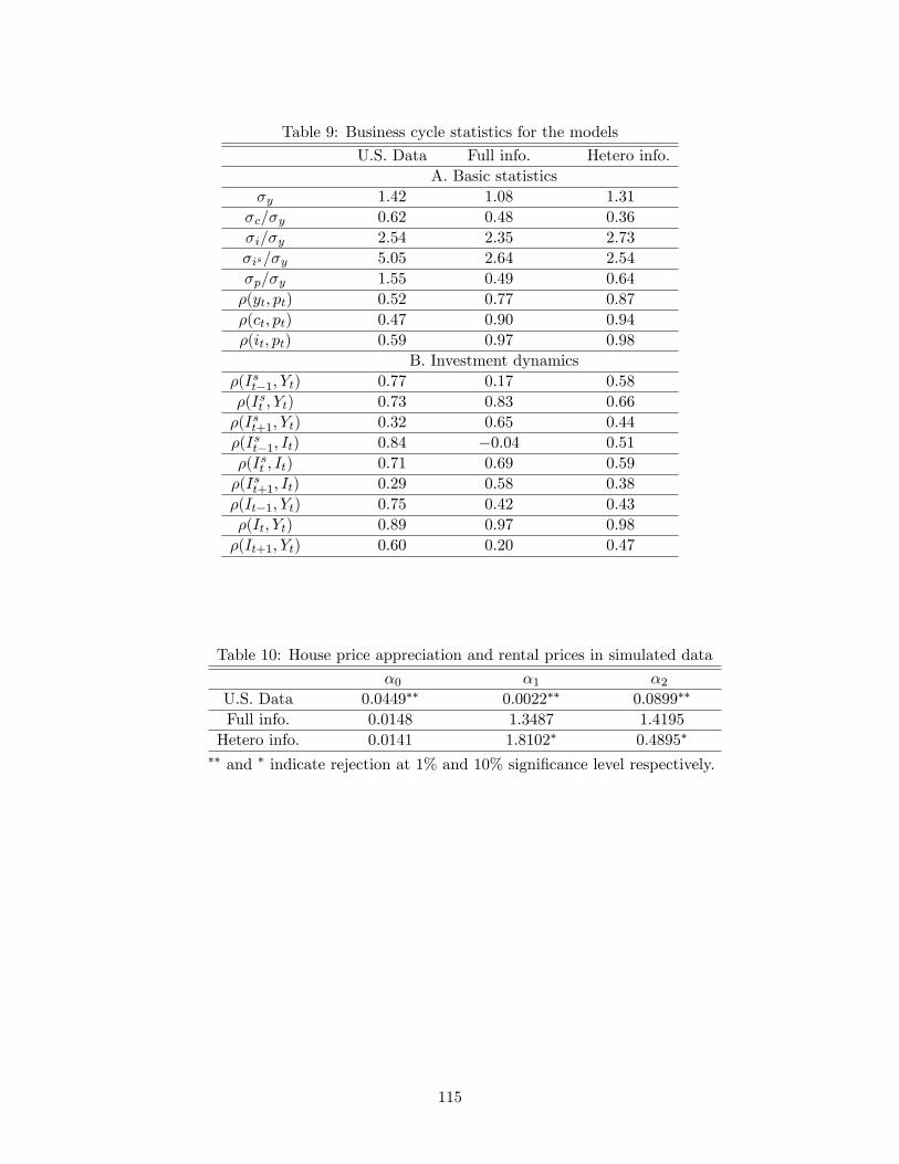
Table 9: Business cycle statistics for the models
U.S. Data Full info. Hetero info.A. Basic statistics
�y 1:42 1:08 1:31
�c=�y 0:62 0:48 0:36
�i=�y 2:54 2:35 2:73
�is=�y 5:05 2:64 2:54
�p=�y 1:55 0:49 0:64
�(yt; pt) 0:52 0:77 0:87
�(ct; pt) 0:47 0:90 0:94
�(it; pt) 0:59 0:97 0:98
B. Investment dynamics�(Ist�1; Yt) 0:77 0:17 0:58
�(Ist ; Yt) 0:73 0:83 0:66
�(Ist+1; Yt) 0:32 0:65 0:44
�(Ist�1; It) 0:84 �0:04 0:51
�(Ist ; It) 0:71 0:69 0:59
�(Ist+1; It) 0:29 0:58 0:38
�(It�1; Yt) 0:75 0:42 0:43
�(It; Yt) 0:89 0:97 0:98
�(It+1; Yt) 0:60 0:20 0:47
Table 10: House price appreciation and rental prices in simulated data
�0 �1 �2U.S. Data 0:0449�� 0:0022�� 0:0899��
Full info. 0:0148 1:3487 1:4195
Hetero info. 0:0141 1:8102� 0:4895�
�� and � indicate rejection at 1% and 10% signi�cance level respectively.
115
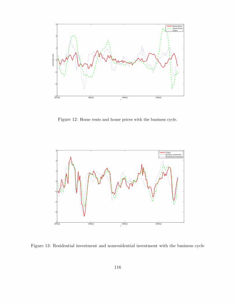
1975Q1 1985Q1 1995Q1 2005Q1−6
−4
−2
0
2
4
6
t
com
mod
ity u
nits
Home RentsHouse PricesOutput
Figure 12: Home rents and house prices with the business cycle.
1975Q1 1985Q1 1995Q1 2005Q1−4
−3
−2
−1
0
1
2
3
t
OutputBusiness InvestmentResidential Investment
Figure 13: Residential investment and nonresidential investment with the business cycle
116
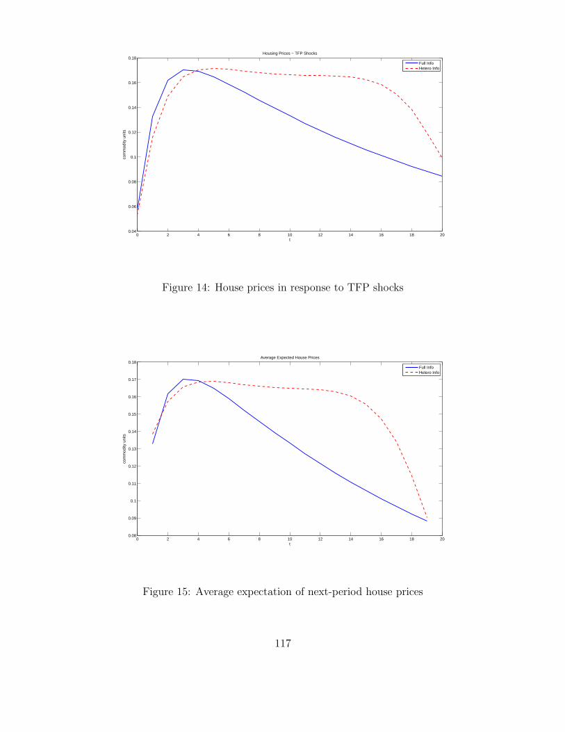
0 2 4 6 8 10 12 14 16 18 200.04
0.06
0.08
0.1
0.12
0.14
0.16
0.18
t
com
mod
ity u
nits
Housing Prices − TFP Shocks
Full InfoHetero Info
Figure 14: House prices in response to TFP shocks
0 2 4 6 8 10 12 14 16 18 200.08
0.09
0.1
0.11
0.12
0.13
0.14
0.15
0.16
0.17
0.18
t
com
mod
ity u
nits
Average Expected House Prices
Full InfoHetero Info
Figure 15: Average expectation of next-period house prices
117
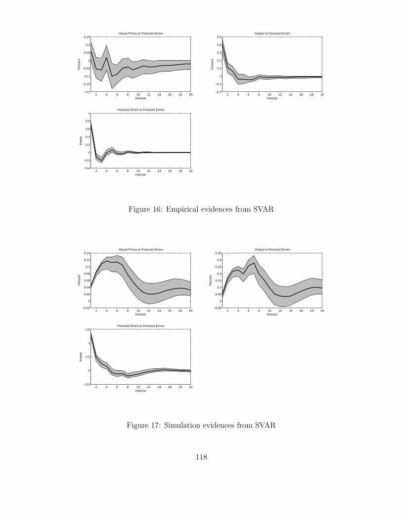
Horizon
Per
cent
House Prices to Forecast Errors
2 4 6 8 10 12 14 16 18 20−0.2
−0.15
−0.1
−0.05
0
0.05
0.1
0.15
Horizon
Per
cent
Output to Forecast Errors
2 4 6 8 10 12 14 16 18 20−0.2
−0.1
0
0.1
0.2
0.3
0.4
0.5
Horizon
Poi
nts
Forecast Errors to Forecast Errors
2 4 6 8 10 12 14 16 18 20−0.4
−0.2
0
0.2
0.4
0.6
0.8
1
Figure 16: Empirical evidences from SVAR
Horizon
Per
cent
House Prices to Forecast Errors
2 4 6 8 10 12 14 16 18 20−0.02
0
0.02
0.04
0.06
0.08
0.1
0.12
0.14
Horizon
Per
cent
Output to Forecast Errors
2 4 6 8 10 12 14 16 18 20−0.05
0
0.05
0.1
0.15
0.2
0.25
0.3
0.35
Horizon
Poi
nts
Forecast Errors to Forecast Errors
2 4 6 8 10 12 14 16 18 20−0.5
0
0.5
1
1.5
Figure 17: Simulation evidences from SVAR
118
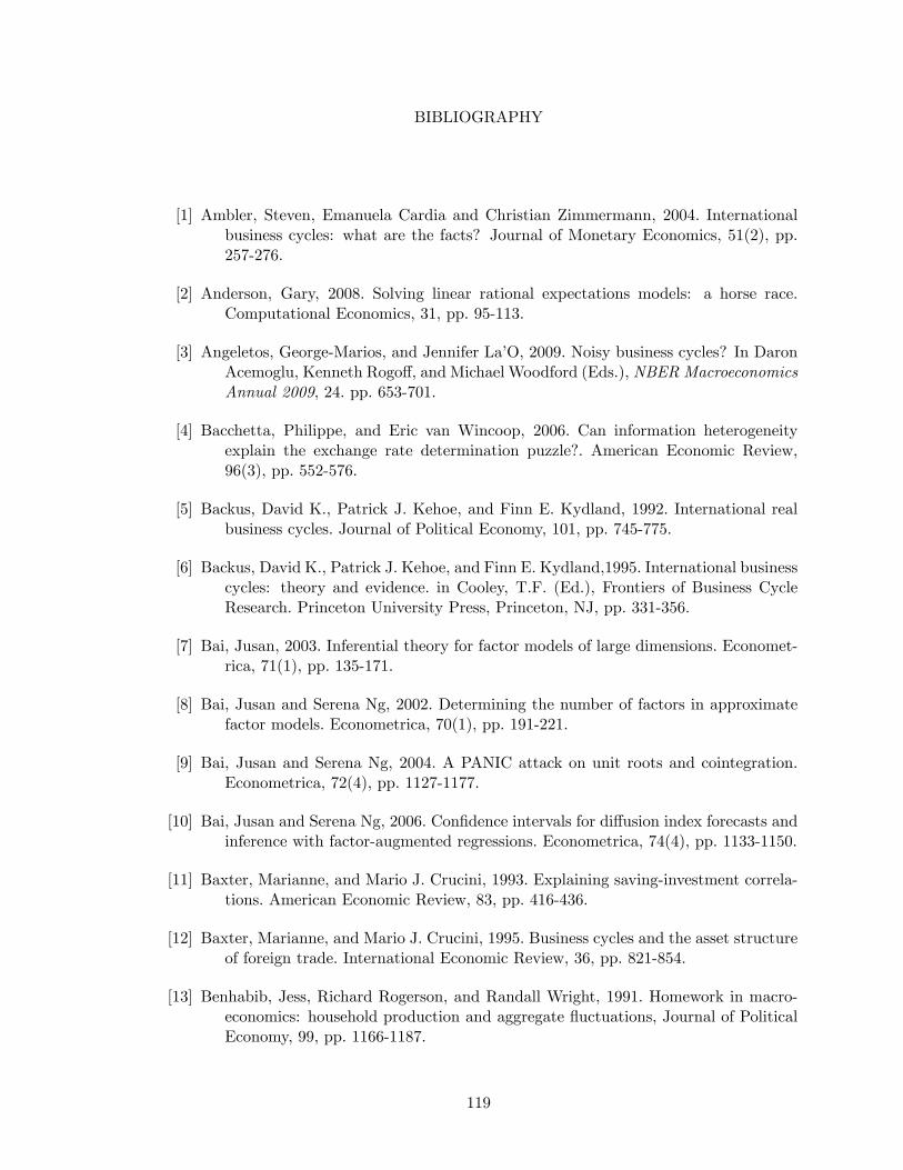
BIBLIOGRAPHY
[1] Ambler, Steven, Emanuela Cardia and Christian Zimmermann, 2004. Internationalbusiness cycles: what are the facts? Journal of Monetary Economics, 51(2), pp.257-276.
[2] Anderson, Gary, 2008. Solving linear rational expectations models: a horse race.Computational Economics, 31, pp. 95-113.
[3] Angeletos, George-Marios, and Jennifer La�O, 2009. Noisy business cycles? In DaronAcemoglu, Kenneth Rogo¤, and Michael Woodford (Eds.), NBER MacroeconomicsAnnual 2009, 24. pp. 653-701.
[4] Bacchetta, Philippe, and Eric van Wincoop, 2006. Can information heterogeneityexplain the exchange rate determination puzzle?. American Economic Review,96(3), pp. 552-576.
[5] Backus, David K., Patrick J. Kehoe, and Finn E. Kydland, 1992. International realbusiness cycles. Journal of Political Economy, 101, pp. 745-775.
[6] Backus, David K., Patrick J. Kehoe, and Finn E. Kydland,1995. International businesscycles: theory and evidence. in Cooley, T.F. (Ed.), Frontiers of Business CycleResearch. Princeton University Press, Princeton, NJ, pp. 331-356.
[7] Bai, Jusan, 2003. Inferential theory for factor models of large dimensions. Economet-rica, 71(1), pp. 135-171.
[8] Bai, Jusan and Serena Ng, 2002. Determining the number of factors in approximatefactor models. Econometrica, 70(1), pp. 191-221.
[9] Bai, Jusan and Serena Ng, 2004. A PANIC attack on unit roots and cointegration.Econometrica, 72(4), pp. 1127-1177.
[10] Bai, Jusan and Serena Ng, 2006. Con�dence intervals for di¤usion index forecasts andinference with factor-augmented regressions. Econometrica, 74(4), pp. 1133-1150.
[11] Baxter, Marianne, and Mario J. Crucini, 1993. Explaining saving-investment correla-tions. American Economic Review, 83, pp. 416-436.
[12] Baxter, Marianne, and Mario J. Crucini, 1995. Business cycles and the asset structureof foreign trade. International Economic Review, 36, pp. 821-854.
[13] Benhabib, Jess, Richard Rogerson, and Randall Wright, 1991. Homework in macro-economics: household production and aggregate �uctuations, Journal of PoliticalEconomy, 99, pp. 1166-1187.
119
[14] Beran, Rudolf and Muni S. Srivastava, 1985. Bootstrap tests and con�dence regionsfor functions of a covariance matrix. Annals of Statistics, 13, pp. 95-115.
[15] Bernanke, Ben, Jean Boivin and Piotr Eliasz, 2005. Measuring the e¤ects of monetarypolicy: A factor-augmented vector autoregressive (FAVAR) approach. QuarterlyJournal of Economics, 120(1), pp. 387-422.
[16] Bryan, Michael F. and Stephen G. Cecchetti, 1993. The consumer price index as ameasure of in�ation, Federal Reserve Bank of Cleveland Economic Review, pp.15�24.
[17] Boileau, Martin and Michel Normandin, 2008. Closing international real businesscycle models with restricted �nancial markets. Journal of International Moneyand Finance, 27, pp. 733-756.
[18] Boivin, Jean and Marc Giannoni, 2006. DSGE models in a data-rich environment.NBER Working Paper no. 12772.
[19] Boivin, Jean and Serena Ng, 2006. Are more data always better for factor analysis?Journal of Econometrics, 132, pp. 169-194.
[20] Bose, Arup, 1988. Edgeworth correction by bootstrap in autoregressions. Annals ofStatistics, 16, pp. 1709-1722.
[21] Bulow, Jeremy, and Paul Klemperer, 1994. Rational frenzies and crashes. Journal ofPolitical Economy, 102, pp. 1-23.
[22] Burnside, Craig, Martin Eichenbaum, and Sergio Rebelo, 2011. Understanding boomsand busts in housing markets, mimeo.
[23] Caplin, Andrew, and John Leahy, 2011. Trading frictions and house price dynamics.Journal of Money, Credit, and Banking, 43, pp. 283-303.
[24] Chaney, Thomas, David Sraer, and David Thesmar, 2012. The collateral channel:how real estate shocks a¤ect corporate investment, American Economic Review,102, pp. 2381-2409.
[25] Chang, Yongsung, 2000. Comovement, excess volatility, and home production. Journalof Monetary Economics, 46, pp. 385-396.
[26] Chari, V.V., Patrick J. Kehoe and Ellen R. McGrattan, 2002. Can sticky price modelsgenerate volatile and persistent real exchange rates?. Review of Economic Studies,69, pp. 533-563.
[27] Chatterjee, Satyajit, and Burcu Eyigungor, 2011. A quantitative analysis of the UShousing and mortgage markets and the foreclosure crisis, mimeo.
[28] Christiano, Lawrence J., Martin Eichenbaum, and Evans, 2005, Nominal rigidities andthe dynamic e¤ects of a shock to monetary policy. Journal of Political Economy,113, pp. 1-45.
120
[29] Christiano, Lawrence J., Martin Eichenbaum, and Robert Vigfusson, 2003. Whathappens after a technology shock? NBER Working Paper 9819.
[30] Clark, Todd E., 2006. Disaggregate evidence on the persistence of consumer pricein�ation. Journal of Applied Econometrics, 21, pp. 563�587.
[31] Cogley, Timothy, and James M. Nason, 1995. Output dynamics in real-business-cyclemodels. American Economic Review, 85, pp. 492-511.
[32] Connor, Gonnor and Robert A. Korajczyk, 1986. Performance measurement with theArbitrage Pricing Theory: A new framework for analysis. Journal of FinancialEconomics, 15, 373-394.
[33] Connor, Gonnor, Robert A. Korajczyk and Oliver B. Linton, 2006. The common andspeci�c components of dynamic volatility. Journal of Econometrics 132(1), pp.231-255.
[34] Crucini, Mario J., Mototsugu Shintani, and Takayuki Tsuruga, 2010. Accountingfor persistence and volatility of good-level real exchange rates: the role of stickyinformation. Journal of International Economics, 81(1), pp. 48-60.
[35] Crucini, Mario J., Mototsugu Shintani, and Takayuki Tsuruga, 2012. Noisy informa-tion, distance and law of one price dynamics across US cities, mimeo.
[36] Davis, Morris A., and Jonathan Heathcote, 2005. Housing and the business cycle.International Economic Review, 46, pp. 751�84.
[37] Davis, Morris A., and Jonathan Heathcote, 2007. The price and quantity of residentialland in the United States. Journal of Monetary Economics, 54, pp. 2595-2620.
[38] Davis, J. Scott, and Kevin X.D. Huang, 2011. International real business cycles withendogenous markup variability. Journal of International Economics, 85, pp. 302-315.
[39] Diebold, Francis X., 2000. �Big Data�dynamic factor models for macroeconomic mea-surement and forecasting. manuscript presented at World Congress of the Econo-metric Society 2000.
[40] Favilukis, Jack, Sydney C. Ludvigson, and Stijn Van Nieuwerburgh, 2011. The macro-economic e¤ects of housing wealth, housing �nance, and the limited risk-sharingin general equilibrium, mimeo.
[41] Fisher, Jonas D., 2007. Why does household investment lead business investment overthe business cycle?. Journal of Political Economy, 115, pp. 141-168.
[42] Freedman, David, 1984. On bootstrapping two-stage least-squares estimates in sta-tionary linear models. Annals of Statistics, 12, pp. 827-842.
121
[43] Galí, Jordi, 1999. Technology, employment, and the business cycle: do technologyshocks explain aggregate �uctuations? American Economic Review, 89(1), pp.249-271.
[44] Gangopadhyay, Kausik, and Juan Carlos Hatchondo, 2009. The behavior of house-hold and business investment over the business cycle, Federal Reserve Bank ofRichmond Economic Quarterly, 95, pp. 269-288.
[45] Gertler, Mark, and Nobuhiro Kiyotaki, 2010. Financial intermediation and creditpolicy in business cycle analysis. The Handbook of Monetary Economics, ed. byBenjamin M. Friedman, and Michael Woodford, vol. 3B, pp. 1341-1393. ElsevierScience B.V., Amsterdam, North Holland.
[46] Geweke, John, 1977. The dynamic factor analysis of economic time-series models. inD. J. Aigner and A.S. Goldberger (eds.), Latent Variable in Socioeconomic Models,Amsterdam, North-Holland, pp. 365-387.
[47] Gomme, Paul, Finn E. Kydland, and Peter Rupert, 2001. Home production meetstime to build, Journal of Political Economy, 109, pp. 1115-1131.
[48] Gonçalves, Silvia and Benoit Perron, 2012. Bootstrapping factor-augmented regressionmodels, working paper, University of Montreal.
[49] Gourichas, Pierre-Olivier and Aaron Tornell, 2004. Exchange rate puzzles and dis-torted beliefs. Journal of International Economics, 64(2), pp. 303-333.
[50] Graham, Liam, and Stephen Wright, 2010. Information, heterogeneity and marketincompleteness. Journal of Monetary Economics, 57, pp. 164-174.
[51] Greenwood, Jeremy, and Zvi Hercowitz, 1991. The allocation of capital and time overthe business cycle. Journal of Political Economy, 99, pp. 1188-1214.
[52] Guo, Zi-Yi, and Mototsugu Shintani, 2011. Noisy information, risk sharing and inter-national business cycles, mimeo.
[53] Hall, Peter, 1992. The Bootstrap and Edgeworth Expansion. New York: Springer-Verlag.
[54] Hansen, Gary D., 1997. Technical progress and aggregate �uctuations. Journal ofEconomic Dynamics and Control, 21, pp. 1005-1023.
[55] Heathcote, Jonathan and Fabrizio Perri, 2002. Financial autarky and internationalbusiness cycles. Journal of Monetary Economics, 49, pp. 601-627.
[56] Himmelberg, Charles, Christopher Mayer, and Todd Sinai, 2005. Assessing high houseprices: bubbles, fundamentals and misperceptions, Journal of Economic Perspec-tives, 19, pp. 67-92.
[57] Hurwicz, Leonid, 1950. Least squares bias in time series, in T. Koopmans (ed.) Sta-tistical Inference in Dynamic Economic Models. Wiley, New York, pp. 365-383.
122
[58] Iacoviello, Matteo, 2005. House prices, borrowing constraints, and monetary policy inthe business cycle. American Economic Review, 95, pp. 739-764.
[59] Iacoviello, Matteo, 2010. Housing in DSGE models: �ndings and new directions, inBandt, O. de; Knetsch, Th.; Peµnalosa, J.; Zollino, F. (Eds.), Housing marketsin Europe: a macroeconomic perspective, Berlin, Hidelberg: Springer-Verlag, pp.3-16.
[60] Iacoviello, Matteo, and Stefano Neri, 2010. Housing market spillovers: evidence froman estimated DSGE model. American Economic Journal: Macroeconomics, 2, pp.125-164.
[61] Ireland, Peter N., 2001. Technology shocks and the business cycle: On empiricalinvestigation. Journal of Economic Dynamics and Control, 25, pp. 703�719.
[62] Kehoe, Patrick J. and Fabrizio Perri, 2002. International business cycles with endoge-nous incomplete markets. Econometrica, 70, pp. 907-928.
[63] Kendall, Manfred G., 1954. Note on bias in the estimation of autocorrelation. Bio-metrika, 41, pp. 403-403.
[64] Kilian, Lutz, 1998. Small-sample con�dence intervals for impulse response functions.Review of Economics and Statistics, 80, pp. 218-230.
[65] Kim, Chang-Jin and Charles R. Nelson, 1998. Business cycle turning points, a newcoincident index, and tests of duration dependence based on a dynamic factormodel with regime-switching. Review of Economics and Statistics, 80, pp. 188-201.
[66] King, Robert G., Charles I. Plosser and Sergio T. Rebelo, 1988. Production, growthand business cycles: I. the basic neoclassical model. Journal of Monetary Eco-nomics, 21, pp. 195-232.
[67] Kiyotaki, Nobuhiro, and John Moore, 1997. Credit cycles. Journal of Political Econ-omy, 105, pp. 211-248.
[68] Kiyotaki, Nobuhiro, Alexander Michaelides, and Kalin Nikolov, 2011. Winners andlosers in housing markets. Journal of Money, Credit, and Banking, 43, pp. 255-296.
[69] Kollmann, Robert, 1996. Incomplete asset markets and the cross-country consumptioncorrelation puzzle. Journal of Economic Dynamics and Control, 20, 945-961.
[70] La�O, Jennifer, 2010. Collateral constraints and noisy �uctuations, mimeo.
[71] Liu, Zheng, Pengfei Wang, and Tao Zha, 2013. Land-price dynamics and macroeco-nomic �uctuations. Econometrica, forthcoming.
[72] Lorenzoni, Guido, 2009. A theory of demand shocks. American Economic Review, 99,pp. 2050-2084.
123
[73] Lucas, Robert Jr., 1972. Expectations and the neutrality of money. Journal of Eco-nomic Theory, 4, pp. 103-124.
[74] Ludvigson, Sydney C. and Serena Ng, 2010. A factor analysis of bond risk premia.In A. Ullah and D. E. A. Giles (eds.), Handbook of Empirical Economics andFinance, pp. 313-372.
[75] Luo, Yulei, Jun Nie and Eric R. Young, 2012. Robustness, information-processing con-straints, and the current account in small open economies. Journal of InternationalEconomics, 88, pp. 104-120. .
[76] MacKinnon, James G. and Anthony A. Smith, 1998. Approximate bias correction ineconometrics. Journal of Econometrics, 85, pp. 205-230.
[77] Mackowiak, Bartosz A., and Mirko Wiederholt, 2009. Optimal sticky prices underrational inattention. American Economic Review, 99. pp. 769-803.
[78] Mankiw, N. Gregory, and Ricardo Reis, 2002. Sticky information versus sticky prices:a proposal to replace the New Keynesian Phillips curve. Quarterly Journal ofEconomics, 117, pp. 1295-1328.
[79] Mankiw, N. Gregory, and Ricardo Reis, 2011. Imperfect Information and AggregateSupply. The Handbook of Monetary Economics, edited by B. Friedman and M.Woodford, vol. 3A, pp. 182-230., Elsevier-North Holland.
[80] Marcellino, Marcellino, James H. Stock and Mark W. Watson, 2003. Macroeconomicforecasting in the Euro area: Country speci�c versus area-wide information. Eu-ropean Economic Review, 47, pp. 1-18.
[81] Marriott, Frank. H. C., and James A. Pope, 1954. Bias in the estimation of autocor-relations. Biometrika, 41, pp. 390�402.
[82] Mayer, Christopher, 2011. Housing bubbles: a survey. Annual Review of Economics,3, pp. 559-577.
[83] Mian, Atif, and Amir Su�, 2011. House prices, home equity-based borrowing, and theU.S. household leverage crisis. American Economic Review, 101, pp. 2132-2156.
[84] Moon, Hyungsik R. and Benoit Perron, 2004. Testing for a unit root in panels withdynamic factors. Journal of Econometrics 122, pp. 81-126.
[85] Morris, Stephen and Hyun Song Shin, 2002. Social value of public information. Amer-ican Economic Review, 92, pp. 1521-1534.
[86] Nimark, Kristo¤er, 2008. Dynamic pricing and imperfect common knowledge. Journalof Monetary Economics, 55, pp. 365-382.
[87] Obstfeld, Maurice and Kenneth Rogo¤, 2000. The six major puzzles in internationalmacroeconomics: is there a common cause? in Bernanke, Ben; Rogo¤, Kenneth
124
(Ed.), NBER Macroeconomics Annual 2000, The MIT Press, Cambridge MA, pp.339-390.
[88] Pakko, Michael, 2004. A spectral analysis of the cross-country consumption correlationpuzzle. Economics Letters, 84, pp. 341-347.
[89] Phelps, Edmund S., 1970. Introduction: the new macroeconomics in employmentand in�ation theory. In Microeconomic Foundations of Employment and In�ationTheory, edited by Edmund et al. Phelps. New York: Norton.
[90] Piazzesi, Monika, and Martin Schneider, 2009. Momentum traders in the housingmarket: survey evidence and a search model. American Economic Review: Papers& Proceedings, 99, pp. 406-411.
[91] Quenouille, Michael H., 1949. Approximate tests of correlation in time series. Journalof the Royal Statistical Society, Series B, 11, pp. 68�83.
[92] Rupert, Peter, and Etienne Wasmer, 2012. "Housing and the labor market: timeto move and aggregate unemployment," Journal of Monetary Economics, 59, pp.24-36.
[93] Sargent, Thomas J. and Christopher A. Sims, 1977. Business cycle modeling withoutpretending to have too much a priori theory. In C. Sims (ed.), New Methods ofBusiness Cycle Research. Minneapolis: Federal Reserve Bank of Minneapolis.
[94] Schmitt-Grohé, Stephanie and Martín Uribe, 2003. Closing small open economy mod-els. Journal of International Economics, 61, pp. 163-185.
[95] Shintani, Mototsugu, 2005. Nonlinear forecasting analysis using di¤usion indexes: Anapplication to Japan. Journal of Money, Credit, and Banking, 37(3), pp. 517-538.
[96] Shintani, Mototsugu, 2008. A dynamic factor approach to nonlinear stability analysis.Journal of Economic Dynamics and Control, 32(9), pp. 2788-2808.
[97] Sims, Christopher. A., 2001. Solving linear rational expectations models. Computa-tional Economics, 20, pp. 1-20.
[98] Sims, Christopher A., 2003. Implications of rational inattention. Journal of MonetaryEconomics, 50, pp. 665-690.
[99] Sterk, Vincent, 2010. Home equity, mobility, and macroeconomic �uctuations. DeNederlandsche Bank and University of Amsterdam, mimeo.
[100] Stock, James H. and Mark W. Watson, 1989. New indexes of coincident and leadingeconomic indicators. In O. Blanchard and S. Fischer (eds.), NBER Macroeco-nomics Annual (Cambridge, Mass. MIT Press).
[101] Stock, James H. and Mark W. Watson, 1998. Di¤usion indexes. NBERWorking Paperno. 6702.
125

[102] Stock, James H. and Mark W. Watson, 2002. Macroeconomic forecasting using di¤u-sion indexes. Journal of Business and Economic Statistics 20, pp. 147-162.
[103] Stockman, Alan and Linda Tesar, 1995. Tastes and technology in a two-country modelof the business cycle: explaining international comovements. American EconomicReview, 85, pp. 168-185.
[104] Townsend, Robert M., 1983. Forecasting the forecasts of others. Journal of PoliticalEconomy, 91, pp. 546-588.
[105] Woodford, Michael D. 1999. Optimal monetary policy inertia, NBER Working Paperno. 7261.
[106] Woodford, Michael D., 2003. Imperfect common knowledge and the e¤ects of mon-etary policy, In Knowledge, Information and Expectations in Modern Macroeco-nomics: In Honor of Edmund S. Phelps, edited by Phillipe Aghion et al.
[107] Yamamoto, Yohei, 2012. Bootstrap inference for impulse response functions in factor-augmented vector autoregressions. working paper, University of Alberta.
126