Embed Size (px)
Citation preview

No. 2007–38
STRATEGIC R&D WITH KNOWLEDGE SPILLOVERS AND
ENDOGENOUS TIME TO COMPLETE
By R. Lukach, P.M. Kort, J. Plasmans
June 2007
ISSN 0924-7815

Strategic R&D with Knowledge Spillovers and
Endogenous Time to Complete
Lukach, R.1, Kort, P.M.2,1, Plasmans, J.1,2
1Department of Economics, University of Antwerp,2Department of Econometrics & Operations Research and
CentER, Tilburg University.
November 22, 2006
Abstract1
We present a model where firms make competitive decisions about the op-timal duration (or time to build) of their R&D projects. Choosing its project’sduration, the firm can choose to become a leader or a follower, based on its R&Defficiency, the size of the R&D to be carried out and the degree of innovation,which this research will produce.
It is shown that asymmetry in R&D efficiency between firms is an importantfactor determining feasibility of the preemption and attrition scenarios in com-petitive R&D with time to build. Scenarios of attrition and preemption gamesare most likely to occur when competitors have similar R&D efficiencies. Incase of largely asymmetric firms the games of attrition and preemption are veryunlikely, thus the R&D duration choices of firms are determined by the actualtrade-off between the benefits of earlier innovation and the costs of faster R&Dproject completion.
JEL Classification: C72, D21, O31Keywords:R&D Investment, Competition, Preemption, Attrition.
1Corresponding Author: Ruslan Lukach, Department of Economics, University of Antwerp,
Prinsstraat 13, 2000 Antwerp, BELGIUM. Tel: +32-3-220-4008. Fax: +3-3-220-4585. E-mail:
1

1 Introduction
The host of the IO literature in the area of competitive/cooperative R&D in-vestment regarding process innovation (Reinganum (1981), d’Aspremont andJacquemin (1988) (referred below as A&J(88)), Suzumura (1992), and Petit,and Tolwinski (1999)) assumes that R&D investment has an immediate effecton the firm’s production capacity and/or efficiency. This implies that theR&D project is completed instantaneously. Obviously, such a setup ignoresan important property of R&D, which is that an R&D project requires time tocomplete.
Dutta (1997) investigates the problem of optimal budget management of anR&D project, which is carried out in several stages. The paper analyzes anoptimization problem of a single decision maker. Our goal is to analyze thefirms’ R&D investment strategies in a duopolistic setting. We depart from thestatic competitive/cooperative R&D investment A&J(88) model.
In our model we combine the knowledge spillover idea of A&J(88) with anoptimal R&D resource allocation problem setting. (Scherer (1967), Pacheco-de-Almedia and Zemsky (2003)). The Pacheco-de-Almedia and Zemsky’s (2003)discrete-time model is timed in three stages: resolution of uncertainty of du-ration T , capacity investment also of duration T , and a production period ofinfinite length. We assume that the firms operate in a deterministic environ-ment and, therefore, our model has two stages: R&D investment in order todevelop a new production process where the firm has to determine the durationof the R&D process (while producing with old technology) and a productionstage from the moment of R&D completion onwards. It can be assumed as wellthat uncertainty about the volume and the cost of R&D has been resolved inthe previous stages of research, and the firm now considers its project durationdecisions in the final stretch of the innovation process. Our analysis is carriedout in a continous-time setting in the spirit of Scherer (1967).
In the presented model there is a positive relation between the degree ofinnovation and the amount of knowledge to be accumulated in order to achievesuch an innovation. Although there is evidence that major product innovationsdo not necessarily require large amounts of resources and/or research effort (seeBercovitz et al. (1997)), it is almost definitely true for process innovations.The Toyota’ successful introduction of its "lean" auto assembly process (Teece(1996) and Van Biesebroek (2003)) required a substantial amount of resourcesto redesign the whole production system and coordinate it with its numeroussuppliers. Our study shows that, for bigger innovations a marginal increase intotal R&D effort necessary to complete the innovation requires more additionaltime than in the case of a smaller innovation.
The firm’s problem of determining the optimal duration of an R&D projectresembles the ground breaking model of technology adoption timing of Fuden-berg and Tirole (1985), which was extended by works of Dutta et al. (1995),Hoppe and Lehmann-Grube (2001) and (2005), and Hoppe (2000). But un-like in the setting of Fudenberg and Tirole (1985), where a new technology isavailable and becomes adopted against some cost, our model contains an R&D
2

process with endogenous time to complete, while the new technology can onlybecome available after this process is completed. Intermediate innovations cannot, thus, be used productively for the firm.
Also, unlike in studies of technology adoption timing of Katz and Shapiro(1987) and Hoppe and Lehmann-Grube (2001), where earlier adoption meansusage of a less advanced technology, in this model the degree of innovationand R&D duration decisions are uncoupled. We find that our assumption fitsbetter for a cost reducing process innovation, because the company deciding tomodernize its production process almost always has a particular level of costreduction in mind. As an example, consider Intel’s computer chip productionprocess, where each cycle of technological improvement has a goal of cuttingthe production cost of "putting" one transistor on the chip by one half (Marcyk(2002)).
With the degree of innovation not being dependent on time, this study showsthat in the precommitment equilibrium the optimal R&D project duration ofthe leader (the firm, which finishes its R&D first) is the same as the optimalduration of the innovator in a duopoly, where only one firm conducts R&D; andthe optimal R&D project duration of the follower (the firm, which finishes itsR&D second) is the same as the optimal duration of the catching up innovator,facing the opponent who already possesses the new technology.
Furthermore, we investigate the competitive equilibria under conditions ofknowledge spillovers, which create incentives for the firm to finish its R&D laterthan its competitor. Katz and Shapiro (1987) considered firms with differentprofit incentives for innovation and derived the corresponding preemption andwaiting game equilibria under different spillover mechanisms such as licensingand imitation. We find that under conditions of weak knowledge spillovers, apreemption equilibrium is more likely to occur, while the attrition equilibriumwill prevail when the spillovers are strong.
Firms’ payoffs in the preemption equilibrium and in the "war of attrition" aredifferent from the corresponding precommitment cases. In the precommitmentscenarios with exogenous roles the optimal duration of R&D is determined bythe trade-off between the extra profit gain from innovation and the additionalR&D cost from finishing the project sooner. Firms do not consider strategiceffects and the incentives for preemption or attrition.
In the preemption scenario the optimal project durations are set in a waythat the follower is not able to preempt the leader. In such a situation the leadermakes its decisions based on the follower’s incentives to preempt (if the followerhas such incentives). As a result, the winner (leader) has lower payoffs thanin the corresponding precommitment case. In the attrition scenario the winner(follower) must neutralize the other firm’s second mover advantage and give uppart of its profits. But, unlike in the preemption case, where the deviatingfirm has the same payoff as in the original position, in the war of attrition thefirm, which deviates, ends up with higher payoffs than in the original position.The looser in the war of attrition receives some extra benefits by getting a moreextended period of technological leadership. This happens due to the fact thatin our model adopting earlier does not mean that the leader will have a less
3

advanced technology than the follower.In the presented model we consider two asymmetric firms, which have dif-
ferent R&D efficiencies in the form of different per unit marginal cost of R&D.This asymmetry plays a role in determining who will become the leader andthe follower, when feedback equilibria are considered. With a reasonable smallasymmetry in R&D efficiency between firms, the game with endogenous rolescan have preemption or attrition equilibria depending on different values of theparameters. But if one firm has a strong advantage in R&D efficiency overthe other, a preemption or attrition game cannot occur. In such a situationthe more R&D efficient firm is almost always capable of capturing the leadingposition.
This paper is structured as follows; the second section of this study presentsthe model of competitive R&D with time to build and knowledge spillovers. Sec-tions 3, 4, 5 and 6 present solutions of the model for monopoly, one-innovatorduopoly, catching-up innovator duopoly, and the two-innovators duopoly, re-spectively. Conclusions and discussions are presented in Section 7.
2 The Model of R&D with Time to Build
In this section we present the setting and main assumptions for the model of acompetitive R&D in duopoly with time to build and knowledge spillovers.
Let us consider the following scenario. A firm is producing a good with aparticular technology. This production technology can be improved throughprocess innovation, which results in decreasing the marginal cost of production.In the initial state of development, this technology allows the firm to producewith marginal cost A. The firm has all necessary R&D capabilities to imple-ment the required innovation, which will allow it to bring the marginal cost ofproduction down to zero.
The firm knows exactly how much R&D is needed to reach a given level ofproduction efficiency. By engaging in R&D the firm must realize a knowledgegain in order to obtain the new production technology. It takes time to completeeach R&D project. The marginal cost decrease takes place only after the projectis completed (i.e. the knowledge gain is fully realized). There is anothercompeting firm in the market operating under the same set of rules, whichmakes it a duopoly.
Consider an A&J(88)-type problem, where the A&J(88) framework is ex-tended by taking the above conditions into account. Assume that for firm i
completion of an R&D project results in decreasing the marginal productioncost from A to 0.
We assume that the two firms are symmetric in their marginal costs of pro-duction (A1 = A2 = A). Therefore, following the specification of the A&J(88)model, firm i ’s total individual knowledge gain must equal firm i ’s marginalcost of production before innovation, A. In this way we explicitly establish apositive correlation between the degree of process innovation and the knowledgegain necessary to achieve such an innovation.
4

To model the "time to complete", we assume that the firm subdivides thetotal R&D in per-period R&D efforts, so that a completed R&D project (incontinuous space) satisfies
∫n
0
xi(t)dt = A, i = 1,2,
where xi(t) is the knowledge gain of firm i, and n is the total duration of theR&D project.
The firms are assumed to be asymmetric in R&D effectiveness, representedby different R&D efficiency (γ
1�= γ
2). The corresponding present value of
firm i ’s total R&D spending of firm exhibits diminishing returns to R&D andis specified as
Ξi =
γi
2
∫n
0
x2i(t)e−rtdt,
where r is the discount rate.Currently we assume that the outcome of each step of the R&D project is
deterministic. By spending Ξi dollars firm i achieves the projected decrease ofthe marginal production cost of A. After the R&D process is completed, thefirm will continue producing with an upgraded technology from time n onwards.
There are knowledge spillovers present in the market, but unlike in A&J(88),where a part of one firm’s R&D effort is utilized by the other firm immediatelyin the form of extra production cost benefit, in our case only one firm can benefitfrom a knowledge spillover, which is the firm that completes its R&D later thanthe other. Here we make a reasonable assumption that during the projectimplementation stage the firms are capable of protecting their knowledge sothat no information flows occur. Yet, when one firm completes the project andthe R&D output becomes realized (Grossman and Helpman (1990)), the otherfirm will be able to obtain some extra technological knowledge by observing thenew technology or products produced with it.
We assume that this amount of knowledge equals a part of the other firm’stotal knowledge gain. For example, if firm i finishes its R&D as second, it willreceive a knowledge spillover of βA at the moment when firm j completes itsproject, where parameter β (0 < β < 1) here determines the strength or degreeof such a knowledge spillover.
Here we address the problem of determining the optimal project durationtime, given a certain amount of new knowledge needed to complete the project tobe carried out during this time. Currently, we approach this task by consideringa two-stage R&D/production game where the firmmust carry out one innovationcycle to achieve one technological breakthrough.
Two situations can be distinguished: one situation with exogenous firm rolesthat are prescribed beforehand implicitely which firm will become the leader andfinish the R&D process first (precommitment strategies as defined in Reinganum(1981)) In the second situation it is not established beforehand which of the twofirms will finish its R&D first. In the latter case the firm roles are endogenous.
5

First, we derive the solution of the general problem of R&D with time tobuild. Then we consider an open-loop game setting with exogenous roles in casesof one-innovator duopoly, catching-up innovator duopoly, and the two innovatorsduopoly, respectively. The monopoly case is considered as a benchmark. Thefeedback model with endogenous roles is presented later.
3 Solution of General Problem of R&D with
Time to Build
Let us consider a firm which produces with some technology generating the profit
stream π0(q(t)). If this firm invests in R&D it can obtain a new technology,
which will generate the profit stream π1(q(t)) after the innovation is completed.
Innovation requires time to build as set in the above model description.
The problem can then be specified as:
max{n,q(t),x(t)}
π =
n∫
0
[π0(q(t)) − γx2(t)
2]e−rtdt+
∞∫
n
π1(q(t))e−rtdt, (1)
s.t.
n∫
0
x(t)dt = A.
First we maximize this payoff function with respect to q(t) and x(t) for agiven n. This requires maximization of the following corresponding Lagrangian
functions:
max
{q(t),x(t),λ}Lt∈(0,n] = [π0(q(t))− γ
x2(t)
2]e−rt + λ
⎛⎝
n∫0
x(t)dt−A
⎞⎠ , and(2)
max{q(t)}
Lt∈(n,∞) = π1(q(t))e−rt. (3)
The FOCs for maximization of (2) and (3) with respect to q(t) require:
∂π0
∂q= 0 and
∂π1
∂q= 0,
from which we obtain the optimal outputs q∗0 (t) and q∗1 (t). These optimal outputsyield π∗0 and π∗1.
Maximizing (2) with respect to x(t) and given the optimal π∗0 and π∗1 isequivalent to minimizing the total cost of R&D carrying out the project subjectto the project completion constraint:
min{x(t),λ}
HΞ,m = γx2(t)
2e−rt − λ
⎛⎝
n∫0
x(t)dt −A
⎞⎠ . (4)
6

The set of first order conditions is:
∂H
∂x= γx(t)e−rt − λn = 0, (5)
∂H
∂λ=
n∫
0
x(t)dt−A = 0. (6)
From (5) we get x(t) = λnert
γ, which after substitution into (6) yields
λ =
Aγre−rn
n(1− e−rn)and
x∗(t)|
t∈(0,n] =
Are−rn
1− e−rnert. (7)
The time schedule of the R&D effort presented in (7) implies the R&D effortincreases during the project implementation phase. This result is in line withthe finding of Grossman and Shapiro (1986) stating that, due to discounting,R&D expenditures increase.
Introducing our preliminary results into (1) and expanding the integrals weobtain:
max{n}
π =1
r
π0 +e−rn
r
∆π −
γ
2A2
re−rn
1− e−rn, (8)
where ∆π = π1 − π0 is the firm’s profit gain from innovation.The FOCs for solving (8) is:
e−rn[γA2r2 − 2∆π(1− e−rn)2] = 0. (9)
Equation (9) has two nonzero roots in terms of e−rn. But, we are interestedonly in non-negative values of n, which means that we consider only valuese−rn < 1. This leaves only one root of interest, which is:
(e−rn)∗ = 1−A√∆π
√γr2
2(10)
and yields:
n∗
= −1
rln
(1−
A√∆π
√γr2
2
). (11)
4 Monopoly
Here we present a one-firm benchmark case. Consider the firm weighing adecision about the length of the R&D project n, which will result in achievinga marginal production cost decrease of A. After the project is completed, the
7

0.80.60.40.20
30
25
20
15
10
5
0
A
n
A
n
Figure 1: Monopolist’s project duration as a function of the degree of innova-tion/knowledge gain (r = 0.05, γ = 10).
firm will be able to produce with a lower marginal production cost from time nonwards. The inverse market demand function is specified as
p = 1− q.
Solving the monopolist’s problem results in the following optimal values of out-
put:
q∗
0,m(t) =
1−A
2, (12)
q∗1,m
(t) =1
2,
with optimal R&D schedule:
x∗m(t) =
Are−rn∗
m
1− e−rn
∗
m
ert,
and an optimal R&D project duration of:
n∗
m= −
1
rln
(1−
√2Aγr2
2−A
). (13)
Additionally, the profits gain from the monopolist’s innovation is ∆πm =
2A−A2
4.
8
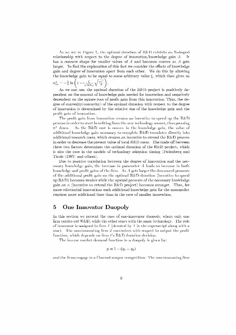
As we see in Figure 1, the optimal duration of R&D exhibits an S-shapedrelationship with respect to the degree of innovation/knowledge gain A. Ithas a concave shape for smaller values of A and becomes convex as A getslarger. To find the explanation of this fact we consider the effects of knowledgegain and degree of innovation apart from each other. We do this by allowingthe knowledge gain to be equal to some arbitrary value ξ, which then gives us
n∗m= −
1
rln
(1−
ξ√∆πm
√γr2
2
).
As we can see, the optimal duration of the R&D project is positively de-pendent on the amount of knowledge gain needed for innovation and negativelydependent on the square root of profit gain from this innovation. Thus, the de-gree of convexity(concavity) of the optimal duration with respect to the degreeof innovation is determined by the relative size of the knowledge gain and theprofit gain of innovation.
The profit gain from innovation creates an incentive to speed up the R&Dprocess in order to start benefiting from the new technology sooner, thus pressingn∗ down. As the R&D cost is convex in the knowledge gain, the value ofadditional knowledge gain necessary to complete R&D translates directly intoadditional research costs, which creates an incentive to extend the R&D processin order to decrease the present value of total R&D costs. The trade off betweenthese two factors determines the optimal duration of the R&D project, whichis also the case in the models of technology adoption timing (Fudenberg andTirole (1985) and others).
Due to positive correlation between the degree of innovation and the nec-essary knowledge gain, the increase in parameter A leads to increase in bothknowledge and profit gains of the firm. As A gets larger the downward pressureof the additional profit gain on the optimal R&D duration (incentive to speedup R&D) becomes weaker while the upward pressure of the necessary knowledgegain on n (incentive to extend the R&D project) becomes stronger. Thus, formore substantial innovations each additional knowledge gain for the monopolistrequires more additional time than in the case of smaller innovation.
5 One Innovator Duopoly
In this section we present the case of one-innovator duopoly, where only onefirm carries out R&D, while the other stays with the same technology. The roleof innovator is assigned to firm 1 (denoted by 1 in the superscript along with astar). The non-innovating firm 2 maximizes with respect to output the profitfunction, which depends on firm i ’s R&D duration decision.
The inverse market demand function in a duopoly is given by:
p = 1− (q1 + q2)
and the firms engage in a Cournot output competition. The non-innovating firm
9

has:
π∗1
2=
n1∫
0
π∗1
0,2e−rt
dt +
∞∫
n1
π∗1
1,2e−rt
dt,
where
π∗1
0,2 =
(q∗1
0,2(t)
)2=
(1−A
3
)2
,
π∗1
1,2=
(q∗1
1,2(t)
)2=
(1− 2A
3
)2
.
The innovator firm in its turn has:
π∗1
1=
n∗1
1∫
0
[π∗1
0,1− γ
x∗1
1(t)
2
]e−rt
dt+
∞∫n∗1
1
π∗1
1,1e−rt
dt
with:
π∗1
0,1 =
(q∗1
0,1(t)
)2=
(1−A
3
)2
,
π∗11,1
=
(q∗11,1(t))2
=
(1 +A
3
)2
,
x∗11(t) =
Are−rn∗1
1
1− e−rn
∗1
1
ert, and
n∗1
1= −
1
rln
(1−
√9Aγ
1r2
8
)
The optimal output levels in this scenario give rise to a profit gain from
innovation ∆π∗11=
4A
9.
The relationship between the optimal duration of the R&D of one innovatorand the degree of innovation/knowledge gain is presented in Figure 2. Here theshape of the relationship between knowledge gain/degree of innovation and theoptimal duration of the project for the same parameter values is similar to thatof the monopolist (Figure 1), but has a less prominent S-shape. Indeed, forrelatively large innovations (with A > 2
9) the innovator’s profit gain is higher
than the profit gain of the monopolist, resulting in stronger incentives to keepthe project duration short. If the degree of innovation is small (A ≤ 2
9), the
effect of the profit gain is stronger for the monopolist.
6 "Catching Up" Innovator Duopoly
Here we consider the case where one firm is already in possession of the newtechnology and the other firm decides about developing the new technology
10

10.750.50.250
25
20
15
10
5
0
A
n
A
n
Figure 2: An innovator’s project duration as a function of the degree of inno-vation/knowledge gain (δ = 0.05, γ
1= 10)
in the "catch up" mode. Let us assume that firm 1 produces with the newtechnology and firm 2 must develop one to be able to compete as equal. Firm2 also benefits from the knowledge spillovers βA generated by firm 1, so it mustsatisfy:
n2∫
0
x2(t)dt = (1− β)A.
The corresponding payoffs of the catching up innovator are (the order of indexesin the superscript indicates the order in which firms innovate):
π∗1
2=
n∗1
2∫
0
[π∗1
0,2− γ
x∗12(t)
2
]e−rt
dt +
∞∫n∗1
2
π∗1
1,2e−rtdt,
11

where:
π∗10,2 =
(q∗1
0,2(t)
)2=
(1− 2A
3
)2
,
π∗11,2
=
(q∗1
1,2(t))2
=
(1
3
)2
,
x∗1
2(t) =
(1− β)Are−rn∗1
2
1− e−rn
∗1
2
ert, and
n∗1
2= −
1
rln
(1− (1− β)
√9Aγ
2r2
8(1−A)
)
and the corresponding profit gain from innovation of the catching-up innovator
is ∆π∗12 =
4A(1−A)9
.
The firm that already has the new technology has the following payoff:
π∗11 =
n∗1
2∫
0
π∗1
0,1e−rt
dt +
∞∫
n∗12
π∗1
1,1e−rtdt,
where
π∗1
0,1=
(q∗10,1(t))2
=
(1 +A
3
)2
,
π∗1
1,1=
(q∗10,1(t))2
=
(1
3
)2
.
The relationship between the degree of innovation/knowledge gain and theoptimal duration of R&D is presented in Figure 3. Here we must take intoaccount that there is another parameter, which plays a role in determining theshape of the optimal project duration for the catching-up innovator. Thisparameter is the strength of knowledge spillovers. The stronger the knowledgespillover the smaller the amount of additional knowledge gain is needed, and,thus, the less additional time should be spent on R&D. In Figure 4 it is clearlyvisible that as knowledge spillovers get stronger, the relationship between thedegree of innovation/knowledge gain becomes more concave.
In Figure 3 we observe that the optimal duration curve with respect to theknowledge gain and the degree of innovation in case of the catching-up innovatoris S-shaped with a prominent convex interval. This is explained by the fact that
the profit gain from innovation for the catching-up innovator (∆π∗122 =4A(1−A)
9 )is always smaller than the innovator’s profit gain in the one innovator duopoly(∆π∗11 =
4A9 ). Thus, the catching-up innovator has less incentives to conduct
its R&D fast.
12

0.80.60.40.20
15
12.5
10
7.5
5
2.5
0
A
n
A
n
Figure 3: "Catching-up" innovator’s project duration as a function of the degreeof innovation/knowledge gain (r = 0.05, γ
2= 10, β = 0.2)
0.8 0.6 0.4 0.2 0
10.75
0.50.25
0
8
6
4
2
0
A
beta
A
beta
Figure 4: Optimal project duration of the catching-up innovator as a functionof A and β (r = 0.05, γ
2= 10).
13

7 Two Innovators with Different Project Dura-
tions
After studying the scenarios where only one firm must make the optimal R&Dduration decision, we turn our attention to the case where both firms in duopolyinnovate and set the optimal time to build for the new technology.
First of all, we want to determine the conditions under which two firms willchoose different durations of their R&D, creating in this way the situation whereone firm becomes the first investor, or the leader, and the other becomes thesecond inventor, or the follower. The follower then benefits from the knowledgespillovers generated by the leader.
Let us for now assume that firm 2 is going to spend more time developing
its new technology: n2 > n1. Currently we consider γ1�= γ
2, but we do not
make any assumptions about which of these parameters is greater.
As firm 2 ’s project duration is longer than that of firm 1 we take into account
two main changes in the firms’ profit functions. First, firm 2 will benefit from
the knowledge spillovers generated at the moment after firm 1 completes its
R&D project. Second, during the time period between n1 and n2 firm 1 will
enjoy a technological advantage over firm 2.
The leader’s optimal payoff is expressed as:
πL
1=
nL
1∫
0
[πL0,1 − γ
1
xL1(t)
2
]e−rt
dt+
nF
2∫
nL
1
π∗L
1,1e−rt
dt +
∞∫
nF2
πL1,1e
−rtdt, (14)
where
πL0,1 =
(qL0,1(t)
)2=
(1−A
3
)2
,
π∗L1,1 =
(q∗L1,1(t)
)2=
(1 +A
3
)2
,
πL1,1 =
(qL1,1(t)
)2=
(1
3
)2
,
xL1(t) =
Are−rnL
1
1− e−rn
L
1
ert, and
nL
1= −
1
rln
(1−
√9Aγ
1r2
8
).
The follower’s optimal payoff is:
πF2=
nL
1∫
0
[πF0,2 − γ
2
xF2(t)
2
]e−rtdt+
nF
2∫
nL
1
[π∗F
0,2− γ
2
xF2(t)
2
]e−rtdt +
∞∫
nF
2
πF1,2e
−rtdt,
(15)
14

with
πF0,2 =
(qF0,2(t)
)2=
(1−A
3
)2
,
π∗F0,2 =
(q∗F0,2(t)
)2=
(1− 2A
3
)2
,
πF1,2 =
(qF1,2(t)
)2=
(1
3
)2
,
xF2(t) =
(1− β)Are−rnF
2
1− e−rn
F
2
ert, and
nF
2= −
1
rln
(1− (1− β)
√9Aγ
2r2
8(1−A)
).
The corresponding profit gains from innovation of the two firms are
∆πL1
=
4A
9,
∆πF2
=4A(1−A)
9.
As the problem is constructed based on the assumption that n2 > n1, thisresult only holds under the parameters requirements, which ensure that nF
2>
nL1. Given δ < 1, it is clear that nF
2> nL
1if and only if
(1− β)2γ2
1−A> γ
1,
orγ2
γ1
>1−A
(1− β)2. (16)
Interpreted directly, expression (16) presents the condition ensuring that thefollower firm will still have to devote more time to complete its R&D than theleader even with the benefit of knowledge spillovers. Such a situation is mostlikely to occur if a notable asymmetry between firms is accompanied by weakknowledge spillovers and a modest degree of innovation.
If (16) does not hold, knowledge spillovers allow the follower to finish itsR&D as soon as the leader completes the project and the knowledge spilloversget realized. In such a case the follower benefits from knowledge created by theleader and does not have a stream of lower profits associated with the periodwhen it lags behind in developing the new technology. Such an outcome occursin case of a smaller asymmetry, strong knowledge spillovers and a small degreeof innovation, which ensure that the second-mover advantage (Hoppe (2000))will be the strongest. Nonetheless, if the roles are exogenously predefined,the leader’s optimal R&D duration choice is not affected by the fact that thefollower will immediately bring up the new technology after the leader.
15
In several limit cases we make the following observations:i)As lim
A→0
β→1
1−A(1−β)2
= ∞ and limA→1
β→1
1−A(1−β)2
= ∞, we conclude that under condi-
tions of strong knowledge spillovers the follower will finish the R&D project atthe same time as the leader.
ii) As limA→0β→0
1−A(1−β)2 = 1 and lim
A→1
β→0
1−A(1−β)2 = 0, we see that with weak knowledge
spillovers the feasible leader-follower arrangement is likely to hold for a broad
range of asymmetries between firms. Moreover, in case of a large degree of
innovation the leader must not be necessarily more efficient in R&D than the
follower, due to a very strong incentive to preempt.
Above we have considered the condition for existence of a unique solution of
the problem where the leader’s role is assigned to firm 1. If the leader’s role isgiven to firm 2, then the unique solution condition requires that
γ1
γ2
>1−A
(1− β)2. (17)
In a situation where both (16) and (17) hold both firms will be able toperform the corresponding functions of the leader/follower, and the equilibriumwill be the result of the game with endogenous roles.
Remark 1 We observe that the leader’s optimal R&D project duration is the
same as the optimal duration of the innovator in the one innovator duopoly:
nL
1= n
∗1
1; and the follower’s optimal R&D project duration is the same as the
optimal duration of the catching up innovator: nF2= n
∗1
2.
Observing results presented in Remark 1 and analyzing firms’ payoff func-tions (14) and (15) we make the following observations. The leader’s optimalR&D project duration based on the profit gain from innovation determined bythe difference in profits in times t ∈ (0, n1] (duopoly with old technology) andtimes t ∈ (n1, n2), where the leader has a technological advantage. Therefore,the decisive factor for the leader is the fact of technological leadership during acertain period of time. The profit stream generated in time periods after bothfirms acquire the new technology is not relevant for the leader’s R&D durationdecisions.
On the other hand, the follower’s optimal R&D duration is based on theprofit gain determined by the difference in profits in times t ∈ (n1, n2] andt ∈ (n2,∞) (duopoly with new technology). Thus, the follower disregards theprofits during the time period when both firms have the old technology andtakes into account the fact that it will be in the inferior position for some time,but will benefit from knowledge spillovers.
In other words, the technological leader will behave (regarding the durationof R&D) as if it is the only innovator in the market with the old technology.On the other hand, the follower will behave as the (catching-up) innovator ina duopoly market where the leader produces with a superior technology. Thisresult is consistent with the findings of Katz and Shapiro (1987), who show that
16
FIRM 2
Follower
NoR&D
FIRM 1
R&D No R&D
7 8
Leader
R&D
FIRM 1
FIRM 2
R&D No R&D R&D No R&D
63
Leader
4
Follower
5
Follower
2
Leader
1
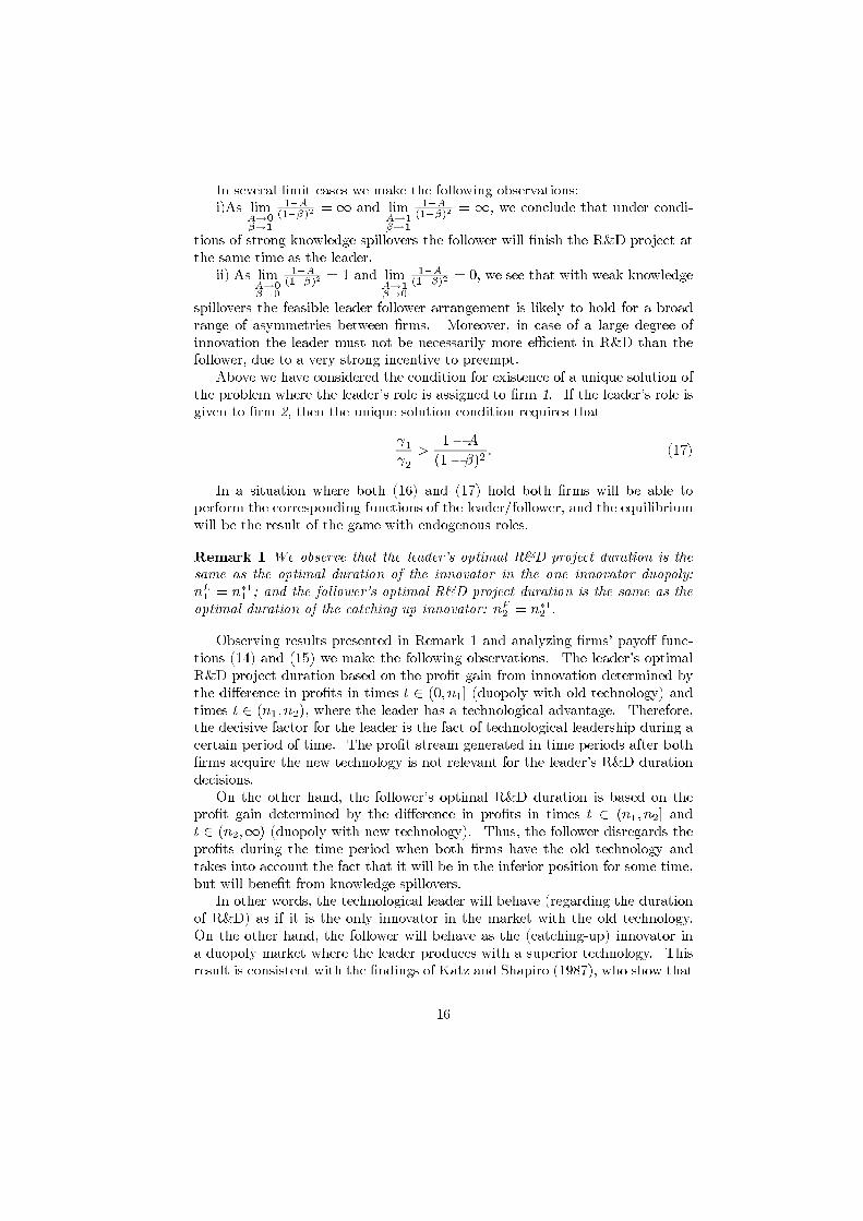
Figure 5: R&D Investment and Timing Decisions Tree.
under conditions of strong imitation risk, the timing of technology adoptionby the leader is not influenced by imitation as long as its leader position ispreserved.
In Appendix we also present the benchmark case of the two innovatorsduopoly with the same project duration, which results will be used in laterdiscussions.
8 Strategy Choice in the Endogenous Roles Game
Here we analyze the firms’ optimal decisions regarding carrying out the R&Dand the mode in which this research must proceed (leader or follower). Inthe leader mode the firm will complete its R&D first, without benefitting fromany positive knowledge spillovers. In the follower mode the firm will completeits innovation as second and will receive an additional benefit in the form ofknowledge spillovers generated by the leader.
We derive the firms’ payoff for each feasible outcome of different leader/followerdecisions in Figure 5, and formulate the firms’ optimal strategies. For simplic-ity purposes we assume that A < 1
2, so that duopoly is preserved in case one
firm does not invest in R&D.It can be shown (see Appendix A??) that firms will finish their R&D projects
simultaneously if and only if they have the same R&D efficiencies. Therefore,for asymmetric firms with γ
1�= γ
2the game will not have the outcome with the
simultaneous completion of R&D.In this game we first consider only the decision paths where each firm chooses
17

the leader/follower role compatible with its competitor’s role, such as on thepaths leading to the outcomes (2), (3), (4), (6), (7), and (8) in Figure 5. Onthe paths corresponding to the outcomes (1) and (5) both firms choose to bethe leader or the follower, respectively. In these cases, one of them must switchits role for the equilibrium to exist. Outcome (1) is a preemption game andin the situation corresponding to outcome (5) a waiting game (war of attrition)takes place.
In this section we derive the firms’ payoffs corresponding to the compatiblerole decisions first, followed by a description of the preemption game and thewaiting game in the outcomes with incompatible role choices.
8.1 Compatible Role Decisions
The compatible role decisions of firms produce the equilibria derived in the sameway as in the scenarios with exogenous roles shown in Sections 5 to 7.
In the outcome (2) the roles of two firms are clearly defined. Firm 1 is theleader and firm 2 is the follower with:
v(2) =
(πL
1
πF
2
),
where
πL
1=
(1−A
3
)21− e
−rnL
1
r−
γ1A2re−rn
L
1
2(1− e−rn
L
1 )+
(1+A
3
)2(e−rn
L
1− e
−rnF
2
r
)
+e−rn
F
2
r
(1
3
)2
,
πF
2=
(1−A
3
)21− e
−rnL
1
r− (1− β)2
γ2A2re−rn
F
2
2(1− e−rn
F
2 )+
(1− 2A
3
)2(e−rn
L
1− e
−rnF
2
r
)
+e−rn
F
2
r
(1
3
)2
,
with nL
1= −
1
rln(1−
√9γ
1Ar2
8),
nF2
= −
1
rln(1− (1− β)
√9γ
2Ar2
8(1−A)).
The outcome (3) presents the situation when only firm 1 invests in R&D:
v(3) =
(π∗1
1
π∗1
2
),
18

where
π∗1
1=
(1−A
3
)2(1− e
−rn∗1
1
r
)+
(1 +A
3
)2e−rn
∗1
1
r,
π∗1
2=
(1−A
3
)2(1− e
−rn∗1
1
r
)+
(1− 2A
3
)2e−rn
∗1
1
r
,
with n∗1
1= −
1
r
ln(1−
√9γ
1Ar2
8).
In the outcome (4) the roles are a reverse of the outcome (2) with firm 1
being the follower and firm 2 being the leader:
v(4) =
(πF
1
πL
2
),
where
πL
2=
(1−A
3
)21− e
−rnL
2
r
−
γ2A2re−rn
L
2
2(1− e−rn
L
2 )+
(1+A
3
)2(e−rn
L
2− e
−rnF
1
r
)
+e−rn
F
1
r
(1
3
)2
,
πF
1=
(1−A
3
)21− e
−rnL
2
r
− (1− β)2γ1A2re−rn
F
1
2(1− e−rn
F
1 )+
(1− 2A
3
)2(e−rn
L
2− e
−rnF
1
r
)
+e−rn
F
1
r
(1
3
)2
,
with nL
2= −
1
r
ln(1−
√9γ
2Ar2
8),
nF1
= −
1
rln(1− (1− β)
√9γ
1Ar2
8(1−A)).
The outcomes (7) and (8) are straightforward and are specified as:
v(7) =
(π∗2
1
π∗2
2
)
where
π∗2
2=
(1−A
3
)2(1− e
−rn∗2
2
r
)+
(1 +A
3
)2e−rn
∗2
2
r,
π∗2
1=
(1−A
3
)2(1− e
−rn∗2
2
r
)+
(1− 2A
3
)2e−rn
∗2
2
r
,
with n∗2
2= −
1
r
ln(1−
√9γ
2Ar2
8).
19

In the outcome (8) both firms decide not to invest in R&D resulting in thestandard Cournot equilibrium with:
q1 = q2 =1−A
3,
π1 = π2 =
(1−A
3
)2 (1
r
),
and
v(8) =
(π1
π2
).
8.2 Preemption Game for Leadership
The decision path leading to the outcome (1) in the game corresponds to thescenario where both firms decide to invest in R&D and want to be the first tofinish research. The profit-maximizing project durations of the two firms are:
nL
1= −
1
r
ln
(1−
√9Aγ
1r2
8
), and
nL2
= −
1
r
ln
(1−
√9Aγ
2r2
8
).
If γ1< γ
2, then n
L
1< n
L
2. Nonetheless firm 2 may attempt to preempt firm
1 by finishing its project a bit earlier as long as the profits obtained in theleader position are higher than the profits of the follower or abandoning theR&D. Firm 1 will follow the same logic and will definitely react to firm 2 ’spreemption attempts. Such a preemption game is illustrated in Figure 6.
As it was mentioned in Remark 1 above, the leader’s project duration in thetwo-innovator duopoly is the same as the duration in the case of one innovator(nL
i= n∗i
i). The after-innovation profits stream of the only innovator is higher
(π∗ii> π
L
i), because the innovating firm has a technology advantage. Thus,
a deviation of one firm from the R&D leadership decision (decision to becomea follower or abandon R&D) will not change the other firm’s decision aboutinvesting in R&D (it will always innovate).
Let us consider some particular value of the R&D project duration n̄ suchthat n̄ < n
L
1and n̄ ≤ n
L
2. Thus, n̄ represents the project duration decision by
which one of the firms tries to preempt the other. Each firm can decrease the
value of n̄ until the profits from preempting become lower than the profits from
becoming a follower or giving up the R&D.
Here the points of interest are the values of n̄ where either firm 1 has:
πL
1
∣∣n̄= π
F
1
∣∣nL
2
, if πF
1≥ π
∗2
1
∣∣nL
2
and πL
1
∣∣n̄= π
∗2
1
∣∣nL
2
, if π∗2
1> π
F
1
∣∣nL
2
(18)
or firm 2 has:
πL
2
∣∣n̄
= πF
2
∣∣nL
1
, if πF
2≥ π
∗1
2
∣∣nL
1
and πL
2
∣∣n̄= π
∗1
2
∣∣nL
1
, if π∗1
2> π
F
2
∣∣nL
1
. (19)
20

1512.5107.55
1
0.875
0.75
0.625
0.5
n
Profits
n
Profits
1Fπ
2Lπ1Lπ
2Fπ
1n 2n1Ln 2
Ln
Figure 6: Preeemption Game Diagram (A = 0.49, γ1= 95, γ
2= 100, β = 0.01,
r = 5%).
The equations in (18) represent the conditions where firm 1 will deviate fromits leader’s decision and will decide to become the follower or not to invest inthe new technology at all. The equations in (19) represent the same conditionsfor firm 2.
To derive which of the two firms will be able to preempt its competitor weneed to explicitly calculate the critical values of duration where the firm willgive up its leader role. These critical values are:
n̄1(nL
2) = max(arg(πL
1
∣∣n̄
= πF
1
∣∣nL
2
),arg(πL1
∣∣n̄= π
∗2
1
∣∣nL
2
)), and (20)
n̄2(nL
1) = max(arg(πL
2
∣∣n̄= π
F
2
∣∣nL
1
),arg(πL2
∣∣n̄
= π∗1
2
∣∣nL
1
)). (21)
Deriving these critical values algebraically results in very complex and non-tractable expressions. Thus, in this study we will use numerical simulations toillustrate some scenarios.
The payoffs corresponding to the preemption outcomes are:
v(1)|π∗1
2>π
F
2
=
(π∗1
1(n̄2)
π∗1
2(n̄2)
), and v(1)|
πF
2≥π∗1
2
=
(πL
1(n̄2)
πF2(n̄2)
), if n̄1 < n̄2, (22)
i.e. when firm 2 deviates first, and
v(1)|π∗2
1>π
F
1
=
(π∗2
1(n̄1)
π∗2
2(n̄1)
), and v(1)|
πF
1≥π∗2
1
=
(πF
1(n̄1)
πL2(n̄1)
), if n̄2 < n̄1, (23)
21
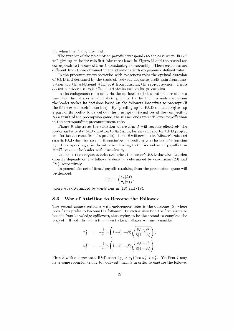
i.e. when firm 1 deviates first.The first set of the preemption payoffs corresponds to the case where firm 2
will give up its leader role first (the case shown in Figure 6) and the second setcorresponds to the case of firm 1 abandoning its leadership. These outcomes aredifferent from those obtained in the situations with exogenously defined roles.
In the precommitment scenarios with exogenous roles the optimal durationof R&D is determined by the trade-off between the extra profit gain from inno-vation and the additional R&D cost from finishing the project sooner. Firmsdo not consider strategic effects and the incentives for preemption.
In the endogenous roles scenario the optimal project durations are set in away that the follower is not able to preempt the leader. In such a situationthe leader makes its decisions based on the followers incentives to preempt (ifthe follower has such incentives). By speeding up its R&D the leader gives upa part of its profits to cancel out the preemption incentives of the competitor.As a result of the preemption game, the winner ends up with lower payoffs thanin the corresponding precommitment case.
Figure 6 illustrates the situation where firm 1 will become effectively theleader and sets its R&D duration to n̄2 (going for an even shorter R&D projectwill further decrease firm 1 ’s profits). Firm 2 will accept the follower’s role andsets its R&D duration so that it maximizes its profits given the leader’s durationn̄2. Correspondingly, in the situation leading to the second set of payoffs firm2 will become the leader with duration n̄1.
Unlike in the exogenous roles scenarios, the leader’s R&D duration decisiondirectly depends on the follower’s decision determined by conditions (20) and(21), respectively.
In general the set of firms’ payoffs resulting from the preemption game willbe denoted:
v(1) =
(π1(n̄)
π2(n̄)
),
where n̄ is determined by conditions in (18) and (19).
8.3 War of Attrition to Become the Follower
The second game’s outcome with endogenous roles is the outcome (5) whereboth firms prefer to become the follower. In such a situation the firm wants tobenefit from knowledge spillovers, thus trying to be the second to complete theproject. If both firms are to choose to be a follower we must consider
nF
2= −
1
r
ln
(1− (1− β)
√9Aγ
1r2
8(1−A)
),
nF2
= −
1
rln
(1− (1− β)
√9Aγ
2r2
8(1−A)
).
Firm 2 with a larger total R&D effort (γ2> γ
1) has nF
2> nF
1. Yet firm 1 may
have some room for trying to "outwait" firm 2 in order to capture the follower
22

17.51512.5107.552.5
2.25
2
1.75
1.5
1.25
n
Profits
n
Profits1Fπ
2Lπ
1Lπ
2Fπ
1n 2n
1Fn
2Fn
Figure 7: Attrition Game Diagram (r = 5%, A = 0.2, γ1= 150, γ
2= 250,
β = 0.8).
position or make it abandon its R&D completely. In case the attrition gametakes place, we conduct comparisons of firms’ profits in different situations tofigure out the outcomes.
Let us define n¯such that n
¯> nF
1and n
¯> nF
2. Duration choice n
¯represents
the decision where one firm tries to extend the time to complete its R&D sothat it will become the follower. As in the preemption game, the other firmmay extend its project’s duration as well in order to outwait its opponent (asshown in Figure 7).
It can be easily seen from (14) that the leader’s payoff is an increasing andconcave function in terms of the follower’s optimal R&D project duration. Thus,the conditions where the firm 1 will give up the follower role in the attritiongame are given by (note that π1 > π∗2
1):
πF
1
∣∣n¯
= πL
1
∣∣n¯
, if πL
1≥ π
∗2
1and π
F
1
∣∣n¯
= π∗2
1
∣∣n¯
, if π∗21
> πL
1. (24)
Correspondingly for firm 2 these conditions are:
πF
2
∣∣n¯
= πL
2
∣∣n¯
, if πL
2≥ π
∗1
2and π
F
2
∣∣n¯
= π∗1
2
∣∣n¯
, if π∗12
> πL
2. (25)
Similarly to the previous case, here different conditions determine differentscenarios and, thus, different solutions of the game. But, unlike in the preemp-tion scenario, deviation of one firm from its decision to invest in R&D as thefollower can lead to a change in the other firm’s decision as well. This happens
23

when one firm decides to abandon it R&D completely. In this case it becomesimpossible for the other firm to be the follower, so it must invest in R&D is theonly innovator or abandon its research too.
Let us define the critical values:
n
¯1(nL
2) = min(arg(πF
1= π
L
1
∣∣n¯
), arg(πF1= π
∗2
1
∣∣n¯
)), and
n
¯2(nL
1) = min(arg(πF
2= π
L
2
∣∣n¯
), arg(πF2= π
∗1
2
∣∣n¯
)).
Consider, for example, the situation when n
¯1 <n
¯2 (as illustrated in Figure
7). Here firm 1 will be the first to deviate from the follower role. If πL1≥ π
∗2
1,
then firm 1 will accept the leader role, with firm 2 as the follower and with firm1 setting its R&D duration equal to n
¯1. On the other hand, observing π∗2
1> π
L
1
firm 1 will abandon its R&D. This will make firm 2 to reconsider its own R&Ddecision. As becoming the follower is no longer feasible, there are two otheroptions left: firm 2 may pursue the innovation alone (if π∗2
2≥ π2), or abandon
its R&D as well (π∗22
< π2). The similar logical sequence is used to determinefirms’ actions if n
¯2 <n
¯1.
The corresponding payoffs of the attrition game:
v(5)|πL
1≥π∗2
1
=
(πL
1(n¯1)
πF
2(n¯1)
), v(5)|
π∗2
1>π
L
1
π∗2
2≥π2
=
(π∗2
1(n¯1)
π∗2
2(n¯1)
),
and v(5)|π∗2
1>π
L
1
π2>π∗2
2
=
(π1
π2
), if n
¯1< n¯2,
or
v(5)|πL
1≥π∗2
1
=
(πF
1(n¯2)
πL
2(n¯2)
), v(5)|
π∗2
1>π
L
1
π∗2
2≥π2
=
(π∗2
1(n¯2)
π∗2
2(n¯2)
),
and v(5)|π∗2
1>π
L
1
π2>π∗2
2
=
(π1
π2
), if n
¯2< n¯1.
Like in the preemption scenario we will use simplified notations for the firms’
payoffs obtained in the game of attrition:
v(5)|πL
1≥π∗2
1
=
(π1(n
¯)
π2(n¯)
)
Firms’ payoffs in the war of attrition are also different from the correspondingprecommitment cases. The winner (follower) has to cancel out the other firm’sincentives to extent its R&D (second mover advantage), thus it has to give uppart of its profits. But, unlike in the preemption case, where the deviating firmhas the same payoff as in the original position, in the war of attrition the firm,which deviates, ends up with the higher payoffs than in the original position.The looser (in this case the leader) receives some extra benefits in the form of a
24
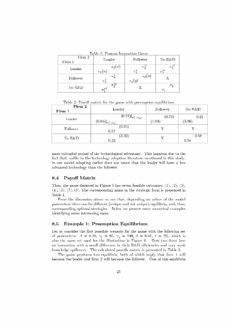
Table 1: Process Innovation GameFirm 2
Firm 1Leader Follower No R&D
Leaderπ2(n̄)
π1(n̄)πF
2
πL
1
π∗1
2
π∗1
1
FollowerπL
2
πF
1
π2(n¯)
π1(n¯)
X
No R&Dπ∗2
2
π∗2
1
Xπ2
π1
Table 2: Payoff matrix for the game with preemption equilibriumFirm 2
Firm 1Leader Follower No R&D
Leader(0.73)|
πF
2(n̄2)
(0.85)|πL
1(n̄2)
(0.73)(1.04)
0.21(3.36)
Follower(0.95)
0.77X X
No R&D(3.32)
0.22X
0.580.58
more extended period of the technological advantage. This happens due to thefact that, unlike in the technology adoption literature mentioned in this study,in our model adopting earlier does not mean that the leader will have a lessadvanced technology than the follower.
8.4 Payoff Matrix
Thus, the game depicted in Figure 5 has seven feasible outcomes: (1), (2), (3),(4), (5), (7), (8). The corresponding game in the strategic form is presented inTable 1.
From the discussion above we see that, depending on values of the modelparameters there can be different (unique and not unique) equilibria, and, thus,corresponding optimal strategies. Below we present some numerical examplesidentifying some interesting cases.
8.5 Example 1: Preemption Equilibrium
Let us consider the first possible scenario for the game with the following setof parameters: A = 0.49, γ
1= 95, γ
2= 100, β = 0.01, r = 5%, which is
also the same set used for the illustration in Figure 6. Here two firms facean innovation with a small difference in their R&D efficiencies and very weakknowledge spillovers. The calculated payoffs matrix is presented in Table 2.
The game produces two equilibria, both of which imply that firm 1 will
become the leader and firm 2 will become the follower. One of this equilibria
25

Table 3: Payoff matrix for the game with attrition equilibriumFirm 2
Firm 1Leader Follower No R&D
Leader X(2.17)
1.420.98
(2.68)
Follower1.20
(2.28)
(1.73)|πF
2(n¯1)
(1.79)|πL
1(n¯1)
X
No R&D(2.53)
1.03X
1.421.42
is equivalent to the precommitment situation and another is produced by a
preemption game. In both equilibria the payoff of the follower is the same and
the leader has a smaller payoff in the preemption equilibrium.
If the roles of the firms are determined endogenously, this particular pa-
rameter setting will produce one Nash equilibrium, which is the preemption
equilibrium. In order to preempt its opponent firm 1 will have to speed up
development resulting in a leader’s payoff decrease of 18%.
8.6 Example 2: Attrition Equilibrium
The next parameters set is: r = 5%, A = 0.2, γ1= 150, γ
2= 250, β = 0.8,
which corresponds to the illustration in Figure 7. In this scenario we see twofirms with notable difference in the R&D production efficiency, which considerinvesting in a relatively small innovation under conditions of strong knowledgespillovers. Numerical calculations give us the payoffs matrix as presented inTable 3.
This game has a unique Nash equilibrium, corresponding to the outcome of awar of attrition. As a result of the waiting game the follower’s payoff decreasedby 25% and the leader’s payoff increased by 26%. In case of precommitmentstrategies, the game would have two leader/follower equilibria and firms wouldface a coordination problem.
8.7 Example 3: No Preemption/Attrition Scenario
To find out the effect of larger asymmetry between firms we consider the fol-lowing parameter set: A = 0.49, γ
1= 50, γ
2= 100, β = 0.01, r = 5%, which is
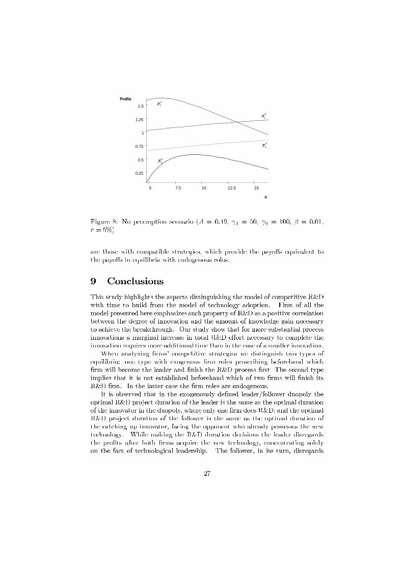
different from that in Example 1 only by a larger degree of asymmetry betweenfirms. From Figures 8 and 9 we can clearly see that neither preemption norwar of attrition are possible.
A very large advantage of a more R&D efficient firm eliminates any pre-emption incentives for the less R&D efficient firm. On the other hand, theknowledge spillover is not strong enough to create the incentive to engage in awaiting game. Thus, it is obvious, that the only outcomes feasible in this game
26
1512.5107.55
1.5
1.25
1
0.75
0.5
0.25
n
Profits
n
Profits
1Fπ
2Lπ
1Lπ
2Fπ
Figure 8: No preemption scenario (A = 0.49, γ1= 50, γ
2= 100, β = 0.01,
r = 5%)
are those with compatible strategies, which provide the payoffs equivalent tothe payoffs in equilibria with endogenous roles.
9 Conclusions
This study highlights the aspects distinguishing the model of competitive R&Dwith time to build from the model of technology adoption. First of all themodel presented here emphasizes such property of R&D as a positive correlationbetween the degree of innovation and the amount of knowledge gain necessaryto achieve the breakthrough. Our study show that for more substantial processinnovations a marginal increase in total R&D effort necessary to complete theinnovation requires more additional time than in the case of a smaller innovation.
When analyzing firms’ competitive strategies we distinguish two types ofequilibria: one type with exogenous firm roles prescribing beforehand whichfirm will become the leader and finish the R&D process first The second typeimplies that it is not established beforehand which of two firms will finish itsR&D first. In the latter case the firm roles are endogenous.
It is observed that in the exogenously defined leader/follower duopoly theoptimal R&D project duration of the leader is the same as the optimal durationof the innovator in the duopoly, where only one firm does R&D; and the optimalR&D project duration of the follower is the same as the optimal duration ofthe catching up innovator, facing the opponent who already possesses the newtechnology. While making the R&D duration decisions the leader disregardsthe profits after both firms acquire the new technology, concentrating solelyon the fact of technological leadership. The follower, in its turn, disregards
27

22.52017.51512.5107.55
2
1.5
1
0.5
0
-0.5 n
Profits
n
Profits
1Fπ
2Lπ
1Lπ
2Fπ
Figure 9: No attrition scenario (A = 0.49, γ1= 50, γ
2= 100, β = 0.01, r = 5%)
the profits where both firms have the old technology and takes into account itstechnological handicap resulting from slower innovation. This emphasizes theimportance of strategic effects for the firms’ R&D duration decisions.
We find that with weak knowledge spillovers the feasible leader-followerarrangement is likely to hold for a broad range of asymmetries between firms.Moreover, in case of a large degree of innovation the leader must not be neces-sarily more efficient in R&D than the follower, due to a very strong incentive topreempt.
With a reasonably small asymmetry in R&D efficiency between firms, thegame with endogenous roles can have preemption or attrition equilibria depend-ing on the parameter constellations. But if one firm has strong advantage inR&D efficiency over another, preemption game and/or attrition games becomenot feasible, thus the more R&D efficient firm is capable of securing its techno-logical leadership.
28

10 APPENDIX
10.1 Two Innovators, Same Project Duration Duopoly Case
Consider firms’ competitive R&D and production strategies provided that to
complete the project they have different R&D efficiencies, but must carry out
their R&D during the same period of time. In this case none of the firms is
able to make use of knowledge spillovers occurring after completion of R&D.
We, thus, assume that firms have γ1�= γ
2, and n1 = n2 = n.
Solving the firm i’s optimal time to build problem we obtain the optimal
payoffs of:
π∗i=
n∗
i∫
0
[π∗
0,i − γx∗i (t)
2
]e−rt
dt +
∞∫n∗
i
π∗
1,ie−rtdt, i, j = 1, 2, i �= j,
and where:
π∗
0,i =
(q∗
0,i(t))2
=
(1−A
3
)2
,
π∗
1,i =
(q∗1,i(t)
)2=
(1
3
)2
,
x∗i (t) =Are−rn∗
i
1− e−rn
∗
i
ert, and
n∗
i= −
1
r
ln
(1−
√9Aγ
ir2
8
)
for i, j = 1,2, i �= j.
It is clearly visible that if γi�= γj, the model does not provide an equilibrium
solution with n∗i = n∗j . Therefore we conclude that it is not optimal for the two
firms with different R&D efficiency to choose the same R&D project durations.
11 References
d’Aspremont, C. and A. Jacquemin (1988), Cooperative and NoncooperativeR&D in Duopoly with Spillovers, The American Economic Review, Vol. 78, pp.1133-1137.
Bercovitz, J., J. de Figueiredo, and D. Teece (1997), Firm Capabilities andManagerial Decision Making: A Theory of Innovation Biases, in R. Garud,P. Nayyar, and Z. Shapira, (eds.), Technological Innovation. Oversights and
Foresights, Cambridge University Press, Cambridge.Dutta P. (1997), Optimal Management of an R&D Budget, Journal of Eco-
nomic Dynamics and Control, Vol. 21, pp. 575-602.
29

Dutta, P., S. Lach, and A. Rustichini (1995), Better Late than Early: Verti-cal Differentiation in the Adoption of a New Technology, Journal of Economicsand Management Strategy, Vol. 4, pp. 563—589.
Fudenberg, D. and J. Tirole (1985), Preemption and Rent Equalization inthe Adoption of New Technology, The Review of Economic Studies, Vol. 52, pp.383—401.
Grossman, G. and E. Helpman (1990), Trade, Innovation, and Growth,American Economic Review, Vol. 80, pp. 86-91.
Grossman, G. and C. Shapiro (1986), Optimal Dynamic R&D Programs,RAND Journal of Economics, Vol. 17, pp. 581-593.
Hoppe, H. (2000), Second-Mover Advantages in the Strategic Adoption ofNew Technology under Uncertainty, International Journal of Industrial Orga-nization, Vol. 18, pp. 115-138.
Hoppe, H. and U. Lehmann-Grube (2001), Second-mover Advantages in Dy-namic Quality Competition, Journal of Economics and Management Strategy,Vol. 10, pp. 419-433.
Hoppe, H. and U. Lehmann-Grube (2005), Innovation Timing Games: AGeneral Framework with Applications, Journal of Economic Theory, Vol. 121,pp. 30-50.
Katz, M. and C. Shapiro (1987), R&D Rivalry with Licensing and Imitation,The American Economic Review, Vol. 77, pp. 402-420.
Marcyk, G. (2002), Silicon Technology: Scaling for the Second Half of theDecade, Logic Technology Development, Intel Corporation (http://intel.com/labs/).
Pacheco-de-Almedia, G. and P. Zemsky (2003), The Effect of Time-to-Buildon Strategic Investment under Uncertainty, RAND Journal of Economics, Vol.34, pp. 166-182.
Petit, M. L. and B. Tolwinski (1999), R&D Cooperation or Competition?,European Economic Review, Vol. 43, pp. 185-208.
Reinganum, J. (1981), Dynamic Games of Innovation, Journal of EconomicTheory, Vol. 25, pp. 21-41.
Scherer, F (1967), Research and development resource allocation under ri-valry, The Quarterly Journal of Economics, Vol. 81, pp. 359-394.
Suzumura, K. (1992), Cooperative and Noncooperative R&D in an Oligopolywith Spillovers, The American Economic Review, Vol. 82, pp. 1307-1320.
Teece, D. (1996), Firm Organization, Industrial Structure, and TechnologicalInnovation, Journal of Economic Behavior and Organization, Vol. 31, pp. 193-224.
Van Biesebroek, J. (2003), Productivity Dynamics with Technology Choice:An Application to Automobile Assembly, The Review of Economic Studies, Vol.70, pp. 167-198.
30