BY - Princeton Universitydeaton/downloads/Saving_and_Liquidity... · Limited borrowing opportunities may also help to explain the observed ... but cannot do so typically can do

Econometrica, Vol. 59, No. 5 (September, 1991), 1221-1248

SAVING AND LIQUIDITY CONSTRAINTS

BY ANGUS DEATON 1

This paper is concerned with the theory of saving when consumers are not permitted to borrow, and with the ability of such a theory to account for some of the stylized facts of saving behavior. When consumers are relatively impatient, and when labor income is independently and identically distributed over time, assets act like a buffer stock, protecting consumption against bad draws of income. The precautionary demand for saving interacts with the borrowing constraints to provide a motive for holding assets. If the income process is positively autocorrelated, but stationary, assets are still used to buffer consumption, but do so less effectively and at a greater cost in terms of foregone consumption. In the limit, when labor income is a random walk, it is optimal for impatient liquidity constrained consumers simply to consume their incomes. As a consequence, a liquidity constrained representative agent cannot generate aggregate U.S. saving behavior if that agent receives aggregate labor income. Either there is no saving, when income is a random walk, or saving is contracyclical over the business cycle, when income changes are positively autocorrelated. However, in reality, microeconomic income processes do not resemble their average, and it is possible to construct a model of microeconomic saving under liquidity constraints which, at the aggregate level, reproduces many of the stylized facts in the actual data. While it is clear that many households are not liquidity constrained, and do not behave as described here, the models presented in the paper seem to account for important aspects of reality that are not explained by traditional life-cycle models.

KEYWORDS: Saving, liquidity constraints, assets, income, dynamic programming.

INTRODUCTION

THIS PAPER IS CONCERNED with the optimal intertemporal consumption behavior of consumers who are restricted in their ability to borrow to finance consumption. The restriction is not a symmetric one. Nothing prevents, these consumers from saving and accumulating assets, and under some circumstances they will find it desirable to do so. Such models are worth pursuing if only because borrowing constraints seem to be a feature of reality, both in poor and rich countries. Furthermore, at least some of the recent econometric work on life-cycle rational expectations models of consumption has discovered anomalies that can perhaps be attributed to consumers' inability to borrow. For the United States, using macroeconomic data, Flavin (1981) and many subsequent authors have found evidence that changes in consumption are positively related to predictable changes in income. The microeconomic evidence, primarily from the Panel Study of Income Dynamics (PSID), is more mixed, but Hall and Mishkin (1982) and Zeldes (1989a) found a relationship between changes in food

1 Fisher-Schultz Lecture, Econometric Society European Meetings, Munich, September 6, 1989. Much of the material in Section 2 of this paper could not have been written without the advice

and assistance of Jim Mirrlees. I am grateful to him for his permission to include our joint work in this lecture. I am grateful to the Lynde and Harry Bradley Foundation and the Pew Charitable Trusts for financial support. I should like to thank Nancy Stokey for her detailed comments on earlier versions, as well as Joe Altonji, Orazio Attanasio, John Campbell, Avinash Dixit, Duncan Foley, Fumio Hayashi, Ian Jewitt, Miles Kimball, Guy Laroque, Greg Mankiw, Steve Pischke, Nick Stem, Steve Zeldes, and two referees for helpful comments and discussion. I alone am responsible for errors.

1221

1222 ANGUS DEATON

consumption and previously predictable income changes, although the work of Altonji and Siow (1987) and Mariger and Shaw (1988) shows that the relationship is not present in all years. Although there is room for different interpreta- tions of these results, the possibility of liquidity constraints has been widely canvassed.

Limited borrowing opportunities may also help to explain the observed patterns of household wealth holdings as well as the fact that consumption appears to track household income quite closely over the life-cycle; see in particular Carroll and Summers (1989). Most versions of life-cycle models predict a dissociation of consumption from income, and the existence of substantial asset accumulations at least at some points in the life cycle. In recent controversies starting with Kotlikoff and Summers (1981) the validity of these predictions has been challenged. In particular, it is clear that most households in the U.S. hold very few assets. Different surveys give somewhat different estimates, but the Survey of Income and Program Participation (SIPP), the Consumer Expenditure Survey (CES), and the Survey of Consumer Finances (SCF) are in broad agreement that median household wealth, excluding pension rights and housing, is around $1000. Indeed, the CES data show that approxi- mately one fifth of total consumption is accounted for by households who not only possess no stocks or bonds, but who have neither a checking nor a savings account. It is hard to believe that such households would be able to borrow much money to finance consumption, should they indeed wish to do so.

In this paper I consider the behavior of relatively impatient consumers, who prefer consumption now to consumption later, and who are unpersuaded by the rewards of waiting. With no uncertainty, and no borrowing constraints, such households would borrow or run down assets. What makes their behavior interesting is that their incomes are uncertain. In common with recent work by Barsky, Mankiw, and Zeldes (1986), Skinner (1988), Zeldes (1989b), and Kimball (1990), I assume that consumers are "prudent" and have a precautionary demand for saving. Precautionary motives interact with liquidity constraints because the inability to borrow when times are bad provides an additional motive for accumulating assets when times are good, even for impatient consumers.

My general procedure is to start from a simple stochastic process for labor income, and to derive, from that process, the appropriate policy rule for consumption given that borrowing is not allowed, or at least cannot exceed some fixed limit. I then focus on the time-series behavior of consumption, savings, and asset accumulation in response to the forcing behavior of income. I shall discuss whether it is possible to build a representative agent model of a liquidity constrained consumer that could account for the main features of the aggregate time-series data in the U.S. But my more fundamental concern is to characterize the type of microeconomic behavior that borrowing constraints might produce. The approach is one of partial equilibrium, and in particular, I make no attempt to model the determination of the real interest rate. I also do not consider the welfare consequences of borrowing restrictions; interested

SAVING AND LIQUIDITY CONSTRAINTS 1223

readers may consult Imrohoroglu (1989) who examines welfare issues in a closely related model.

The analysis shows that, in the presence of borrowing restrictions, the behavior of saving and asset accumulation is quite sensitive to what consumers believe about the stochastic process generating their incomes. In the simplest case, when incomes are stationary and independently and identically distributed over time, as might be the case for a poor farmer in a developing country, assets play the role of a buffer stock, and the consumer saves and dissaves in order to smooth consumption in the face of income uncertainty. I show that it is possible to make consumption very much smoother than income without borrowing and without accumulating very many assets. The more prudent are consumers, and the more uncertain is income, the greater is the demand for these precautionary balances.

Positive serial correlation in the income process diminishes both the desirability and the feasibility of using assets in this way. In the limit, when income is a random walk, with or without drift, it turns out that those who wish to borrow but cannot do so typically can do no better than consume their incomes. This "rule-of-thumb" or simple Keynesian policy is not generally optimal in the presence of borrowing constraints, but the random walk case is one of several income processes that produce the result. I also investigate the consequences of borrowing restrictions in an environment in which income growth is stationary, but where the growth rates mimic aggregate data and are positively serially correlated. These models produce what may appear to be the paradoxical result that, when consumers follow the optimal consumption policy, savings is contracyclical, rising at the onset of the slump, when incomes are falling, and falling at the onset of the boom, when incomes are rising.

In reality, microeconomic income processes are very different from their macroeconomic aggregates, so that while individual consumers share in the general growth, the variance in their incomes is dominated by idiosyncratic components, some permanent, some transitory. The presence of substantial transitory income at the individual level is quite likely to generate negative serial correlation in individual income growth rates, and this can generate buffering behavior as in the simple models with no growth. If each agent's income process is independent of all others, such behavior will not generate savings in the aggregate. However, some component of aggregate fluctuations in income growth is common to all consumers, and even though it accounts for only a very small fraction of individual income changes, its existence can generate savings in the aggregate. I construct a simple model in which individual income growth is negatively autocorrelated, aggregate income growth is positively autocorrelated, and aggregate saving is procyclical.

For much of the analysis, I shall assume an infinite horizon. This is mostly for technical convenience in that it allows me to derive relatively simple stationary policy rules, but the contrast with finite life models is more apparent than real. The existence of borrowing constraints effectively shortens the horizon, and in many cases, the infinite horizon policy rule will characterize much of the finite

1224 ANGUS DEATON

plan, in the same way that finite horizon growth models possess turnpike growth paths that are themselves the solutions to infinite horizon problems. In cases where this is not true, the solutions are typically already covered in the literature, so that a fairly complete treatment is possible.

There are two main sections to the paper. In the first, I assume that the process generating labor income is stationary, while the second deals with the nonstationary case. The analysis differs markedly in the two cases. Section 1.1 outlines the basic model, and 1.2 shows how to incorporate serial correlation within the stationary model. Section 2.1 is concerned with the case in which income growth is independently and identically distributed over time. Section 2.2 allows for serial dependence in the growth process, and is concerned with the behavior of liquidity constrained consumers whose income process mimics that of U.S. aggregate data. Section 2.3 examines income processes that more closely mirror the microeconomic data and considers the implication of individual behavior for the aggregate.

1. SAVING AND LIQUIDITY CONSTRAINTS WITH STATIONARY INCOME

1.1. The Basic Model

The framework is the standard one of intertemporal utility maximization. The consumer maximizes the utility function

(1)~~~~~~~~~~~~D (1) u = Ett E (1 + 6)t tv(c"))

where 8 > 0 is the rate of time preference, and v(ct) is the instantaneous (sub)utility function, assumed to be increasing, strictly concave, and differen- tiable. The evolution of assets is given by

(2) At+1 = (1 + r)(At + -ct)

where yt is labor income, At is real assets, and r is the real interest rate. The real interest rate is treated as fixed and known, and all the uncertainty is focussed on labor income yt. Labor is inelastically supplied, and y, is a stationary random variable with support [y0, y1], with y0 > 0 and y 0 y1 < 00; income cannot fall below the positive floor yo. I take the simplest form for the borrowing restriction

(3) At>0 although it would be straightforward to allow for some fixed negative limit.

Since it will be used so much in what follows, I shall denote the instantaneous marginal utility of money by A(cd), i.e.

(4) A(ct) = v'(ct).

A(-) is a positive monotone decreasing function. In most of what follows I shall assume a precautionary motive for saving by taking A(-) to be convex. A decrease in consumption causes the "price" of consumption to rise by at least as


much as an increase reduces it, so that increased uncertainty (and Jensen's inequality) raises the expected price of future consumption relative to that of current consumption.

Rather more attention has to be given to my next assumption, that 8 > r. For many people, particularly those close to subsistence in LDC's, the assumption seems to me to be a natural one, and one that is worth following through. However, much of the standard empirical life-cycle literature is premised on the supposition that 8 = r. While the assumption is probably more favored for its convenience than its inherent plausibility, there are undoubtedly many individuals who are sufficiently patient to ensure that 8 S r. I therefore consider briefly the various possible configurations of interest and impatience; readers interested in more detail can consult the papers by Schechtman (1975), Bewley (1977), Schechtman and Escudero (1977), and Mendelson and Amihud (1982).

Take first the case where 8 = r = 0. Schechtman (1975) has shown that, if this is so, and with the income process independently and identically distributed over time, consumption will converge to the mean of income, ,u, say. Such a result is possible in spite of the liquidity constraints, because the optimal policy results in At tending to infinity as t becomes large. Bewley (1977) has shown that this version of the permanent income hypothesis also holds if Schechtman's i.i.d. assumption is extended to stationarity. In some ways this is an attractive model; consumption is smooth, indeed completely so, and assets act as a buffer against fluctuations in income. However, in reality, consumption does fluctuate with income, if not one for one, and we do not observe consumers responding to liquidity constraints by accumulating indefinitely large quantities of assets.

Consumers for whom 8 S r will accumulate assets indefinitely, and in the limit, the income stream becomes irrelevant as consumption comes to be financed increasingly out of capital income. Borrowing constraints are unlikely to be of relevance for such consumers; saving, not borrowing, is their main concern. Dynasties and central planners apart, such infinite horizon models are not very relevant for individual consumers. More interesting results are obtained by working with a finite horizon. With no uncertainty, and a constant income stream, these patient consumers will accumulate early in life and decumulate later, so that, once again, borrowing constraints are not an issue. With uncertainty, and with convex marginal utility, more assets will be accumulated early in life, consumption will begin from a lower level and will grow more rapidly, so that, once again, borrowing constraints are unlikely to be binding. The solutions to these problems (without liquidity constraints) have been studied by Skinner (1988) and Zeldes (1989b); their simulations show that there can be substantial precautionary accumulation if future incomes are sufficiently uncertain. Again, we have the problem that, unless income happens to match the desired consumption stream, the assumption that 8 < r generates more accumulation than appears to be the case for many consumers. For example, in occupations with uncertain but relatively flat income profiles, consumers should accumulate when they are young; in fact, as in most occupations, consumption tracks income closely; see Carroll and Summers (1989).

1226 ANGUS DEATON

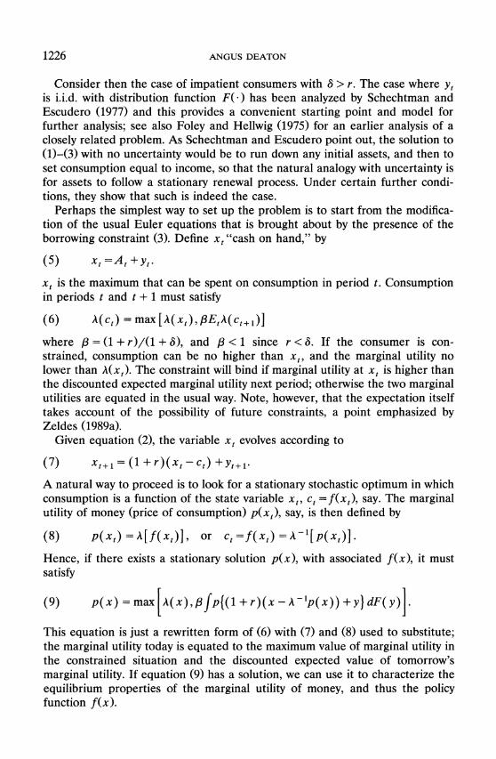
Consider then the case of impatient consumers with 8 > r. The case where y, is i.i.d. with distribution function F(Q) has been analyzed by Schechtman and Escudero (1977) and this provides a convenient starting point and model for further analysis; see also Foley and Hellwig (1975) for an earlier analysis of a closely related problem. As Schechtman and Escudero point out, the solution to (1)-(3) with no uncertainty would be to run down any initial assets, and then to set consumption equal to income, so that the natural analogy with uncertainty is for assets to follow a stationary renewal process. Under certain further conditions, they show that such is indeed the case.

Perhaps the simplest way to set up the problem is to start from the modifica- tion of the usual Euler equations that is brought about by the presence of the borrowing constraint (3). Define x "cash on hand," by

(5) xt =At +Yt.

xt is the maximum that can be spent on consumption in period t. Consumption in periods t and t + 1 must satisfy

(6) A(ct) = max [A(xt), 8EtA(ct+M)

where f3 = (1 + r)/(1 + 8), and f8 < 1 since r < 8. If the consumer is constrained, consumption can be no higher than xt, and the marginal utility no lower than A(xt). The constraint will bind if marginal utility at xt is higher than the discounted expected marginal utility next period; otherwise the two marginal utilities are equated in the usual way. Note, however, that the expectation itself takes account of the possibility of future constraints, a point emphasized by Zeldes (1989a).

Given equation (2), the variable xt evolves according to

(7) xt+1 = (1 + r)(xt -ct) + yt+,.

A natural way to proceed is to look for a stationary stochastic optimum in which consumption is a function of the state variable xt, ct =f(xt), say. The marginal utility of money (price of consumption) p(xt), say, is then defined by

(8) p(xt) =A[ft(xt)], or ct=f(xt) =A-1[p(xt)].

Hence, if there exists a stationary solution p(x), with associated f(x), it must satisfy

(9) p(x)=max[A(x),|fp{(1+r)(x-A'1p(x))+y}dF(y)].

This equation is just a rewritten form of (6) with (7) and (8) used to substitute; the marginal utility today is equated to the maximum value of marginal utility in the constrained situation and the discounted expected value of tomorrow's marginal utility. If equation (9) has a solution, we can use it to characterize the equilibrium properties of the marginal utility of money, and thus the policy function f(x).


The standard method of solving these problems is also useful for thinking about the economics, and about how the infinite horizon solution relates to the same problem with a finite horizon. Imagine a series of functions p0(x), p1(x),.. ., pj(x), where p0(x) A(x), and the updating rule is

(10) Pn(X)=max [A(x),8 fpn{(1+r)(x-A-'Pn(x))+y}dF(y)].

This recursion can be thought of as the backward solution to a finite life stochastic dynamic program. In the final period, n = 0 say, everything is spent, and the marginal utility of money p0(x) is simply A(x) because whatever x is, it will be spent. One period before, p1(x) is set by the borrowing constraints or to equate marginal utilities, and so on back in time. In this form, equation (10) is useful for calculating the functions pn(X) and thus for solving and simulating any finite period problem. Under appropriate conditions, as we iterate back- wards, the function will converge, in which case we have a solution to (9) and to the infinite horizon problem. If we define the mapping T by pn + 1(x) = Tpn(x), then the condition 8 > r, so that 18 < 1, together with the restrictions on the support of F(y), guarantee that T is a contraction mapping; see Theorem 1 of Deaton and Laroque (forthcoming). In consequence, under the original assump- tions, there exist unique functions p(x) and c =f(x) that solve the original problem.

An alternative approach to the same solution is to work through the value function, V(x), defined by the functional equation

(11) V(x) = O?max (v(x-s) + (1 +)' fV[(1 +r)s+y] dF(y)}

where s is the amount of assets held over into the next period. The period by period recursion corresponding to (10) is

(12) Vn(x)= max (v(x-s)+(1+)Y' fVn1[(l+r)s+yJdF(y)}.

The solution to (11) exists under the same conditions as the solution to (9), and the two solutions are linked both by the envelope property p(x) = V'(x) and by the fact that s(x), the argument that maximizes (11), satisfies c = f(x) = x - s(x). Since the value function inherits the concavity of the original utility function v(x), it is monotone increasing and concave, so that we have the useful property that p(x) is decreasing, so that f(x) = A -'{p(x)} is increasing. Deaton and Laroque (forthcoming, Theorem 3) show that the convexity of A(x) implies that p(x) is convex. Without borrowing constraints, it is the convexity of A(x) that controls the degree of precautionary saving. With borrowing constraints, the same role is played by p(x), so the inherited convexity means that the same arguments for prudence and precautionary savings go through when borrowing is prohibited. Indeed, p(x) is more convex than A(x); the inability to borrow in adversity reinforces the precautionary motive.

Mendelson and Amihud (1982) and Deaton and Laroque (forthcoming) also show that there exists a unique x* such that p(x) = A(x) for x <x*, and

1228 ANGUS DEATON

a

0 CN4

0 0

~~~~~~~~~=(/h+rx)/(l1+r) 0

-,0

E cn 0 y is N(100,a), r=O.05, 6=0.10

0

0 coses are from top to bottom

p=2, a=1O and o-=15

? 0 . . , H p=3, a=1 0 aond o- 1 5

0 40 80 120 160 200 240 280 320 income+assets

FIGURE 1.-Consumption functions for alternative utility functions and income dispersions.

p(x) > A(x) for x > x*, so that we have

(13) c=f(x)=X, XsAX*,

c=f(x) Ax, x> x*.

The consumption function therefore has the general shape shown in Figure 1, shown there for y, distributed as N(A, a-), u = 100, r = 0.05, 8 = 0.10, and A(c) = c-. Such figures appear in Mendelson and Amihud (1982) and are "smoothed" versions of the piecewise linear consumption functions derived in the certainty case by Heller and Starr (1979) and Helpman (1981). The figure shows four different consumption functions corresponding to the four combinations of two values of p and o-; they all begin as the 45-degree line, and diverge from it and one another at their respective values of x*, all of which, in this case, are a little below ,u, the mean value of income, shown as a vertical line. The other line in the figure will be discussed below.

The general properties of the solution are clear. Starting from some initial level of assets, the household receives a draw of income. If the total value of assets and income is below the critical level x*, everything is spent, and the household goes into the next period with no assets. If the total is greater than x* , something will be held over, and the new, positive level of assets will be carried forward to be added to the next period's income. Note that there is no presumption that saving will be exactly zero; consumption is a function of x, not of y, and f(x) can be greater than, less than, or equal to y. Assets are not desired for their own sake, but to buffer fluctuations in income. When income is low, there will be dissaving, and when it is high, there will be saving.


Note too that the distribution of consumption will not be symmetric. It is always possible for the consumer to prevent consumption from becoming too high since additional resources can always be carried forward. But the opposite is not true. If cash on hand is sufficiently low, it will be optimal to spend everything; in spite of prudent preferences, money is worth more now than it is expected to be in the future. But there is nothing to stop there being a bad income draw in the next period, and without assets carried forward, consumption cannot be higher than income. Optimal smoothing cannot do much against a series of bad harvests.

The evolution of cash on hand is governed by the equation

( 14) Xt+ 1 = (1 + r) [x X-f( Xt)] + Yt+.

In consequence xt+1 will be less than xt if

(15) ( ('I A ) '<Axt)- (rxt' /)) (1 +r) (1 +r)

so that xt can only go on expanding if the income draw is large enough to offset the vertical difference between f(x) and the line c = (, + rx)/(1 + r) in Figure 1, a difference that is increasing in x. From the graph it would appear that xt cannot become infinitely large, but must eventually collapse. Schechtman and Escudero show that this is true in general for -1 < r < 0, and will be true for all r < 8 provided additional restrictions are placed on the utility function. These restrictions are not satisfied by negative exponential utility (see also Levhari, Mirman, and Zilcha (1980)) but are satisfied by many other utility functions, including the isoelastic case. The evolution of the marginal utility of money p(x,) is also of interest. In the standard case, without borrowing restrictions, p(x,) follows a martingale, whereas in the current case, it follows a renewal process. As long as the consumer carries forward positive assets, we have the martingale result that Ej{p(x?+ 1)) = 8 - 'p(x,), but as soon as assets fall to zero, which they eventually must, the process "loses its memory" and begins again; conditional on zero assets Ej p(x,?+ l)) = E{ p(y)), a constant.

Further results require a more intimate knowledge of the consumption function f(x), and since there is little hope of recovering closed form solutions, it is necessary to use the contraction mapping apparatus to compute the functions over some suitable grid. Equation (10) is one possibility for doing so, but the presence of pn(x) on both right and left hand sides makes the computation extremely cumbersome. In practice, (10) seems to work well when pn(x) on the right hand side is replaced by pn-1(x) and p0(x) is set to A(x). Using Simpson's rule to evaluate the integral, and with a grid of 100 points, the computations were easily done on a 386-series PC, taking 5-20 minutes per calculation depending on the values of the parameters. I also repeated the calculations using the value function (12). In this case, the calculations follow the equation directly, and the policy function is recovered from the value of s(x) at the converged solution. For the problems examined here, this procedure

1230 ANGUS DEATON

0

@ ~~y is N(100,10), r=0.05, d=0.10, p=3

0

C',

aL consumption-40

=-o 0 , ',, ,M!, C Lo

1 0 20 40 60 80 100 120 140 160 180 200

time FIGURE 2.-Simulations of income, consumption, and assets, with white noise income.

was no faster, and although the same results were obtained, there are a number of computational disadvantages to using the value function approach. Firstly, in order to maximize over s for different values of x, it is necessary to have grids for both magnitudes, so that, to get adequate precision, very large matrices are required. Secondly, the utility function is typically not defined for all possible combinations of x and s, specifically those for which x - s is negative, and while this problem is not difficult to deal with, the programming is further complicated. Finally, the use of grids generates a policy function at the final stage that is a step function, which has to be "smoothed" once convergence is obtained. By contrast, the direct approach to the policy function through the modified version of (10) is straightforward to program, and seems to be robust in practice. The real virtue of (12) is that, unlike (10) it can be used in the finite-life case, even with 8 < r, when policy functions must be calculated for each period separately.

Figure 2 shows a 200 period simulation of one of the cases displayed in Figure 1. Income, consumption, and assets are drawn to the same scale. The marginal utility function is c-P, and income is simply 200 random drawings from N(100, 10). Consumption is notably smoother than income; its standard deviation is 4.9 as opposed to 10 for the income process. It is asymmetric, and its downward spikes are much more severe than any corresponding upward peaks. Assets show repeated reversions to zero, although assets are more often held than not. Only along the "flats" at zero is consumption equal to income, something that happens relatively rarely. Note that the level of assets is typically quite low, usually less than 10% or one standard deviation of income. It is an important finding that it is possible to smooth consumption to the extent shown with so few assets. The desirability of doing so is determined by the parameters


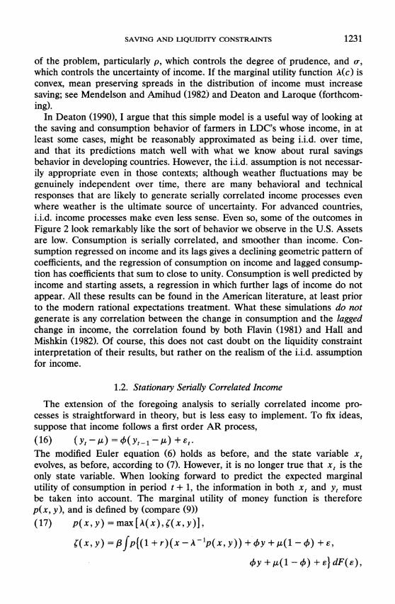
of the problem, particularly p, which controls the degree of prudence, and o-, which controls the uncertainty of income. If the marginal utility function A(c) is convex, mean preserving spreads in the distribution of income must increase saving; see Mendelson and Amihud (1982) and Deaton and Laroque (forthcoming).

In Deaton (1990), I argue that this simple model is a useful way of looking at the saving and consumption behavior of farmers in LDC's whose income, in at least some cases, might be reasonably approximated as being i.i.d. over time, and that its predictions match well with what we know about rural savings behavior in developing countries. However, the i.i.d. assumption is not necessar- ily appropriate even in those contexts; although weather fluctuations may be genuinely independent over time, there are many behavioral and technical responses that are likely to generate serially correlated income processes even where weather is the ultimate source of uncertainty. For advanced countries, i.i.d. income processes make even less sense. Even so, some of the outcomes in Figure 2 look remarkably like the sort of behavior we observe in the U.S. Assets are low. Consumption is serially correlated, and smoother than income. Con- sumption regressed on income and its lags gives a declining geometric pattern of coefficients, and the regression of consumption on income and lagged consumption has coefficients that sum to close to unity. Consumption is well predicted by income and starting assets, a regression in which further lags of income do not appear. All these results can be found in the American literature, at least prior to the modern rational expectations treatment. What these simulations do not generate is any correlation between the change in consumption and the lagged change in income, the correlation found by both Flavin (1981) and Hall and Mishkin (1982). Of course, this does not cast doubt on the liquidity constraint interpretation of their results, but rather on the realism of the i.i.d. assumption for income.

1.2. Stationary Serially Correlated Income

The extension of the foregoing analysis to serially correlated income processes is straightforward in theory, but is less easy to implement. To fix ideas, suppose that income follows a first order AR process, (16) (Y - /)=4(y-_1-/) +e'. The modified Euler equation (6) holds as before, and the state variable xt evolves, as before, according to (7). However, it is no longer true that xt is the only state variable. When looking forward to predict the expected marginal utility of consumption in period t + 1, the information in both xt and yt must be taken into account. The marginal utility of money function is therefore p(x, y), and is defined by (compare (9)) (17) p(x, y) = max [A(x), ?(x, y)],

?(x,y) =,3fp{(1 +r)(x-Ak-p(x,y)) +y +,u(1-4) +e,

by + u(l -4) + e} dF(e),

1232 ANGUS DEATON

and the associated consumption function f(x, y) is given by A - 1{p(x, y)). It is possible to show that, if the autocorrelation parameter 0 is positive, p(x, y) is nonincreasing in y and strictly decreasing when p(x, y) is greater than A(x), and vice versa when 4 is negative. In the former case, a good draw of income indicates that more good draws are to be expected, so that income can be expected to be higher in the future, and more can be spent out of a given amount of cash on hand. With p negative, as for a tree-crop farmer, part of the income from a good crop is really a loan from next year and should be treated accordingly.

In principle, p(x, y) can be computed in exactly the same way as p(x) in the previous subsection. In practice, the additional dimensionality poses difficult computational problems. If an n-point grid is used for each variable, then an n X n grid is required, effectively squaring the computational time. Rather than transfer to a supercomputer, I have chosen to replace the continuous income process by a discrete approximation in a way similar to that suggested by Tauchen (1986).

Suppose that the underlying distribution of ? in (16) is normal, N(O, o-). I first choose (mr-1) points a1, a2, ... , am 1, such that, with ao = -Xo and am = + , the successive areas under the standard normal, rP(aj) - .P(aj-1), are each equal to 1/m. I then take the m conditional means Z1, Z21 ... Zml within each of the intervals as the m equiprobable values of a discrete process that approximates N(O, 1). The true AR(1) for income implies that y, is distributed as N(Ij, 02) where 02 = o.2/(1 _ 22). This is replaced by a discrete first-order Markov process in which income takes on the m discrete values ,u + Ozi, with transition probabilities rij set to be identical to the transition probabilities from interval to interval of the true underlying normal autoregressive process y, From the properties of the normal distribution, we have

(18) rij =Pr(Oaj > -ix > Oaj_ 1Oai >yt-1 1- > Oai-1)

6 ( 2wrr)

x f exp - _ ( '( j-1 dxP ai-I 262 aJP ~ f X

For any given o- and P, this integral is calculated directly. The marginal utility function p(x, y) is then replaced by m functions p(x, i), i= 1,... m, each representing the marginal utility of x given that state i occurs, i.e. that income takes on the value Ozi + ,u. The functions are simultaneously defined by

(19) p(x, i) = max [A(x), E7ijp{(l + r)(x -A-lp(x, i)) + Oz1 + 1 j)]

The computations are as before; I start from po(x, i) = A(x) for all i, substitute into the right hand side of (19), and so on. I used m = 10 in all the calculations reported here and found that convergence was always straightforward. Indeed,


0

o highest state

0

0

4 0

Dn o /

y(t)- 100=0.7(y(t- 1)-1 00)+e(t)

(0 O/ e(t)'~ N(0, 1O), p=2, r-0.02, 6=0.05

0

01

<o /

0 40 80 120 160 200 240 280 320

cash on hand FIGURE 3.-Consumption and cash on hand for AR(1) income process.

the replacement of numerical integration by matrix multiplication appears to more than compensate for the need to compute 10 functions instead of one.

One particular set of consumption functions is shown in Figure 3. These functions are computed for the 10 point discrete Markov approximation with a positive autocorrelation parameter of 0.7. The coefficient of relative risk aversion is 2, the real interest rate 2%, the rate of time preference 5%, and the white noise driving process is N(0, 10). I have also computed similar sets of functions for 4 = ( - 0.4, 0, 0.3, 0.5, 0.7, 0.9); these are not shown, but I will refer to the results in the text.

As was the case when income was i.i.d., the consumption functions each follow the 45-degree line, branching off at critical values of x that depend on the level of income, or the "state." In this example, as in all others with 4 > 0, the lowest consumption function corresponds to the lowest value of income, and vice versa. When 4 = 0, the consumption functions collapse into one, as in Figure 1 (a useful check on the code!), while they move further apart as the autocorrelation increases.

A simulation corresponding to Figure 3 is shown in Figure 4. Careful inspection of the income series shows that there are, indeed, only 10 values; these are most noticeable when there are repeat values with associated troughs or "tables." Once again, consumption is smoother than income, with standard deviations of 10.4 and 14 (13.3 in the sample) respectively. Savings are pro-cyclical, and relatively large asset stocks are occasionally accumulated, particularly after long booms. There are also quite long periods when there are no, or close to no assets, and during which consumption is equal to income. The asymmetric

1234 ANGUS DEATON

0

(1-.7L)(y-100) is N(0,10), r=0.02, d=0.05, p=2

00

0'*0

00

a. consumption-40

0 C)4

(n (0)

0 20 40 60 80 100 120 140 160 180 200 time

FIGURE 4.-Simulations of income, consumption, and assets with positively autocorrelated income.

behavior of consumption is still prominent; savings are a much more effective cushion against high consumption than against low consumption.

The important point to note here is that positive serial correlation in the income process reduces the scope for income smoothing for liquidity constrained consumers. For the range of autocorrelation coefficients examined, the standard deviations of income and consumption are shown in Table I. For the i.i.d. case, optimal smoothing can remove half of the standard deviation of income, and for the negatively autocorrelated case, this figure rises to 57%. By contrast, when incomes have an autocorrelation coefficient of 0.9, consumption is essentially as noisy as income. I can think of several factors that help explain these results. By assumption, these consumers have a rate of time preference in excess of the interest rate, so that assets are costly to hold. The precautionary demand is a powerful motive to hold assets, but the smoothing of consumption over long autocorrelated swings requires more assets, and more sacrifice of consumption, than is the case when income is i.i.d. or negatively autocorrelated.

TABLE I

STANDARD DEVIATIONS OF CONSUMPTION AND INCOME FOR AR(1) INCOME, PARAMETER 4

AR coeff 4 -0.4 0.0 0.3 0.5 0.7 0.9

1. sd(y) 10.9 10.0 10.5 11.5 14.0 22.9 2. estsd(y) 10.8 10.2 10.0 11.4 13.3 27.5 3. est sd(c) 4.6 5.1 6.7 7.6 10.4 25.9 ratio 3/2 0.43 0.50 0.67 0.67 0.78 0.94


Positive autocorrelation also restricts the ability to smooth consumption. Once cash on hand falls below the minimum of the points at which the consumption functions in Figure 3 depart from the 45-degree line, no assets will be held, even if the bad income shock that produced the situation is a signal that further bad draws are to follow. These (anticipated) bad times have to be ridden out without any assets to cushion their impact.

In spite of the (important) difference that autocorrelation makes, the basic insights of the original model carry forward. For impatient consumers in a stationary environment, assets are expensive to hold, but can provide a useful buffer between consumption and income. Such buffers are more effective and less costly the less positively autocorrelated is the income stream. As is the nature of a buffer, savings can be negative as well as positive, and will be procyclical in the usual way. However, it is quite possible that saving will be zero for finite periods of time, something that is more likely the more positively autocorrelated is income.

Many of these results seem to accord well both with intuition (at least with mine) and with most of the stylized facts as we know them. But a serious difficulty remains. Most consumers in developed and developing economies can reasonably expect income to grow over time. As I shall show in the next section, if they do hold such expectations about their own incomes, the analysis may be very different. Of course, growth may not happen that way, and each consumer may expect his or her own income stream to be stationary, with growth taking place only from generation to generation. If so, the analysis of this section goes forward, with aggregate asset growth because the buffer stocks of the young will be larger than the buffer stocks of the old. Standard life-cycle models emphasize low frequency "hump" saving, and generate aggregate saving through aggregation effects when population and income are growing. The models examined here work with "high frequency" saving, and the same sort of aggregation effects will give positive saving and asset accumulation in the aggregate. Of course, the magnitudes will be much smaller than in the traditional story, and that again appears to be in accord with the data.

2. SAVING AND LIQUIDITY CONSTRAINTS WITH NONSTATIONARY INCOME

In this section, I examine the same model of savings with borrowing constraints under the assumption that the logarithm of the income process is stationary in first-differences. Without uncertainty, such an assumption corresponds to steady growth. Here I shall be concerned with logarithmic random walks with drift, as well as with processes whose first differences are either first-order autoregressions or first-order moving averages. Such models are capable of modelling actual aggregate household income in the U.S., and are thus the relevant processes if aggregate consumption is to be treated as that of a representative individual. The "correct" model of individual income is less obvious, but it is nevertheless plausible that many consumers perceive their incomes as displaying stationary growth rates rather than levels.

1236 ANGUS DEATON

2.1. Independent and Identically Distributed Growth

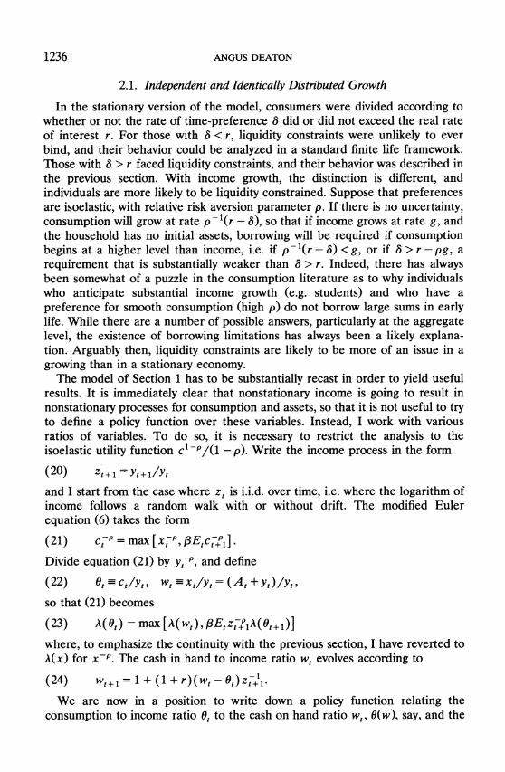
In the stationary version of the model, consumers were divided according to whether or not the rate of time-preference 8 did or did not exceed the real rate of interest r. For those with 8 < r, liquidity constraints were unlikely to ever bind, and their behavior could be analyzed in a standard finite life framework. Those with 8 > r faced liquidity constraints, and their behavior was described in the previous section. With income growth, the distinction is different, and individuals are more likely to be liquidity constrained. Suppose that preferences are isoelastic, with relative risk aversion parameter p. If there is no uncertainty, consumption will grow at rate p - 1(r - 8), so that if income grows at rate g, and the household has no initial assets, borrowing will be required if consumption begins at a higher level than income, i.e. if p- 1(r - 8) < g, or if 8 > r - pg, a requirement that is substantially weaker than 8 > r. Indeed, there has always been somewhat of a puzzle in the consumption literature as to why individuals who anticipate substantial income growth (e.g. students) and who have a preference for smooth consumption (high p) do not borrow large sums in early life. While there are a number of possible answers, particularly at the aggregate level, the existence of borrowing limitations has always been a likely explanation. Arguably then, liquidity constraints are likely to be more of an issue in a growing than in a stationary economy.

The model of Section 1 has to be substantially recast in order to yield useful results. It is immediately clear that nonstationary income is going to result in nonstationary processes for consumption and assets, so that it is not useful to try to define a policy function over these variables. Instead, I work with various ratios of variables. To do so, it is necessary to restrict the analysis to the isoelastic utility function c -P/(1 - p). Write the income process in the form

(20) zt+1=Yt+ 1/Yt

and I start from the case where zt is i.i.d. over time, i.e. where the logarithm of income follows a random walk with or without drift. The modified Euler equation (6) takes the form

(21) c-P = max [ xyP, pEt c71]P Divide equation (21) by y-P, and define

(22) 0tlyt, wt--x/yt = (At + yt)/yt,

so that (21) becomes

(23) A(Ot) =max [A(wt), 8Etz+P

where, to emphasize the continuity with the previous section, I have reverted to A(x) for x-P. The cash in hand to income ratio wt evolves according to

(24) wt+1 = 1 + (1 + r)(wt -Ot)z-+1

We are now in a position to write down a policy function relating the consumption to income ratio Ot to the cash on hand ratio wt, 0(w), say, and the


associated marginal utility p(w) = A{0(w)}. Note that p() is now the "scaled" marginal utility; it is the marginal utility of the wealth to income ratio multiplied by y-P. If the function exists it satisfies (substitute (24) in (23))

(25) p(w) = max[A(w),I8zPP{l + (z1 + r)z-l(w-A7-p(w)))dF(z)].

The question of existence is approached in exactly the same way as before. A finite life analog is constructed, and the backward iteration is set up and used to define a mapping from the policy in period n to that in the previous period n + 1. If this mapping is a contraction mapping, the finite life problem will converge to the infinite period solution given sufficient time. Otherwise, the infinite horizon problem has no solution and the finite life problem must be analyzed directly from the associated value function, exactly as done by Barsky, Mankiw, and Zeldes (1986), Skinner (1988), and Zeldes (1989b). With minor adaptation, the proof of Theorem 1 in Deaton and Laroque (forthcoming) can be used to show that the period to period mapping of the policy function is a contraction if

(26) PE(z-P) = (1 + r)E(z-P)/(1 + 8) < 1.

If this condition holds there will exist a unique optimum policy satisfying (25). If z is lognormally distributed, so that A ln y, is N(g, a 2), and we make the usual approximation that In (1 + r) - In (1 + 8) = r - 8, then (26) becomes

(27) p-'1(r - ) + po2/2 <g.

Condition (26) and its specialization (27) are the conditions that ensure that borrowing is part of the unconstrained plan. For the rest of the analysis, I assume that (26) holds, so that a unique p(w) exists.

The function p(w), defined by (25), and the associated consumption ratio function 0(w) have the same general shape as the consumption functions in Figure 1 although with an origin of (1, 1), not (0,0). As before, there exists some critical level of w, w* say, such that, for w < w*, p(w) = A(w) and 0(w) = w. The ratio wt evolves according to the process

(28) Wt+1= 1 +zT+1(l +r){wt-A 1p(wt)}

so that as soon as wt falls to w* or below, w+1 is 1. But p(l) = 1, because 1 < w*, or directly from substitution in (25) and using (26), so that once wt is 1, it remains 1 thereafter, no matter what are the future values of income. A value of wt of unity implies that assets are zero, so that once assets fall to zero, they remain zero. In this case, with consumption equal to income, it may readily be confirmed that (26) is (over)sufficient to guarantee that expected utility is bounded, or alternatively, that the appropriate transversality condition is satisfied.

1238 ANGUS DEATON

What appears to be more difficult to dispose of is the case where the consumer begins with some assets, since it is not clear to me that there could not exist a distribution F(z) which would generate a p(w) in (28) that would keep w permanently above w*. In special cases, this can be ruled out. Since p(w,) is monotone nondecreasing, and p(w) > A(w), with equality for w < w*, p(w) <p(w*) = A(w*), so that AW1{p(wd)} < w*. Define a, = w, - 1 > 0, and the stochastic process bt, such that bo = ao, and

(29) b+1 =z11(l + r)(bt - b*)

where b* = w* - 1 > 0. Now wt - 1 = at < bt for all t. Hence, if {bt} eventually falls below b*, then {wtj must be below w*, and will thus fall to unity in the next period. If w* were unity, which is its lowest possible value, the logarithm of bt would follow a random walk with drift ln (1 + r)/(1 + g)); recall that (1 + g) is the expectation of ln zt. Hence, if g > r, ln (bt) is a random walk with zero or negative drift, and will in finite time fall below b*, forcing wt below w* and thence to unity. Even if g < r, the quantity b* is nonnegative, so there are clearly other cases where, from an initial asset position, assets will quickly collapse to zero. However, I have not been able to develop a set of necessary conditions to guarantee that assets always collapse. In all the simulations that I have run, and from many different starting values, wt S w* after only a few periods, and I conjecture that this happens in general. If this is the case, the complete solution to the consumer's problem is that, if there are any opening assets, they will decline to zero in finite time, and thereafter consumption will be equal to income. In the case where the logarithm of income is a random walk, with or without drift, and provided (26) holds, then we get the often cited (but not generally valid) consequence of liquidity constraints, that consumption equals income.

When income is a random walk, we have the limiting case of the autoregressive stationary model in the previous subsection, and the presence of binding borrowing constraints makes it undesirable to undertake any smoothing. To see what is going on, suppose that the consumer has no assets, but that income growth is well above average. At first thought, this seems like a good situation to save. But, by assumption, the consumer is already liquidity constrained and the additional income merely provides an opportunity to get closer to the ideal consumption path that would have been realized had there been no borrowing constraints. So good draws in the income growth process are spent, and assets remain at zero. Saving is also typically desirable when income is expected to be lower in the future; see particularly Campbell (1987). However, with a random walk, while a bad draw does indeed imply that income thereafter can be expected to be permanently lower, the expected growth rate of income is unchanged, and nothing can signal a future trough in income over which it would be desirable to maintain consumption by accumulating assets now. There is never any rational expectation that income will be lower than it is now. In consequence, the combination of the persistence of the random walk and the binding liquidity constraints precludes the accumulation of assets.


2.2. Autocorrelated Growth and the Cycle

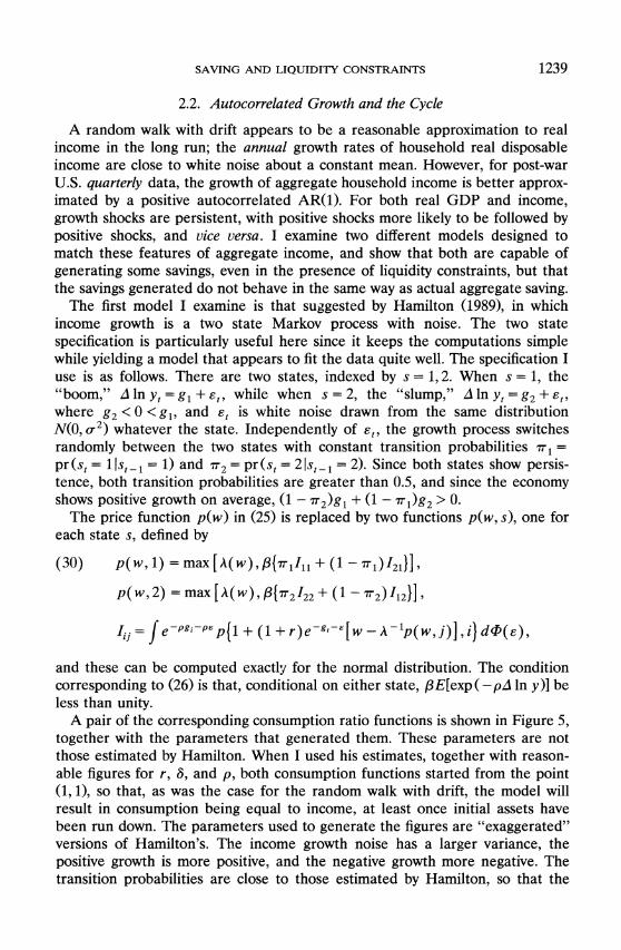
A random walk with drift appears to be a reasonable approximation to real income in the long run; the annual growth rates of household real disposable income are close to white noise about a constant mean. However, for post-war U.S. quarterly data, the growth of aggregate household income is better approximated by a positive autocorrelated AR(1). For both real GDP and income, growth shocks are persistent, with positive shocks more likely to be followed by positive shocks, and vice versa. I examine two different models designed to match these features of aggregate income, and show that both are capable of generating some savings, even in the presence of liquidity constraints, but that the savings generated do not behave in the same way as actual aggregate saving.

The first model I examine is that suggested by Hamilton (1989), in which income growth is a two state Markov process with noise. The two state specification is particularly useful here since it keeps the computations simple while yielding a model that appears to fit the data quite well. The specification I use is as follows. There are two states, indexed by s = 1,2. When s = 1, the "boom," A ln y, = g1 + E, while when s = 2, the "slump," A ln yt = g2 + E1, where g2 <0 <g1, and E, is white noise drawn from the same distribution N(O, ar2) whatever the state. Independently of Et, the growth process switches randomly between the two states with constant transition probabilities 7r= pr (st = 1 st - 1 = 1) and 7n2 = pr (st = 2 1st - 1 = 2). Since both states show persistence, both transition probabilities are greater than 0.5, and since the economy shows positive growth on average, (1 - r2)g1 + (1 - r1)g2 > O

The price function p(w) in (25) is replaced by two functions p(w, s), one for each state s, defined by

(30) p(w, 1) = max [A(w),(3{(71Ijj + (1 -l),211],

p(w,2) = max [A(w),13{r2122 + (1 -72) 12}],

Iij= e-Pgi-Pep{l + (1 + r)e-g,-'[w-A-lp(w,j)],i) dO(E),

and these can be computed exactly for the normal distribution. The condition corresponding to (26) is that, conditional on either state, f3E[exp (-pA ln y)] be less than unity.

A pair of the corresponding consumption ratio functions is shown in Figure 5, together with the parameters that generated them. These parameters are not those estimated by Hamilton. When I used his estimates, together with reasonable figures for r, 6, and p, both consumption functions started from the point (1, 1), so that, as was the case for the random walk with drift, the model will result in consumption being equal to income, at least once initial assets have been run down. The parameters used to generate the figures are "exaggerated" versions of Hamilton's. The income growth noise has a larger variance, the positive growth is more positive, and the negative growth more negative. The transition probabilities are close to those estimated by Hamilton, so that the

1240 ANGUS DEATON

0

o Alny(t)=4%+e in the boom

O o h lny(t)=-3%?t in the slump e is N(0,.02), p=2, r=6=0.10

O ?~ boom consumption

0 o

0_ /

o s tntion probability is 0.8

suboom retention probobility is 0.9 a) 6 1.01 1.02 1.03 1.04 1.05 1.06 1.07 1.08 1.09 1.10

cash on hand to income ratio FIGURE 5.-Consumption to cash on hand ratios for Hamilton's model.

autoregressive properties of the income growth process are similar to those found in the data.

The important results are in Figure 6, which shows a 200 period simulation of the saving ratio, the ratio of assets to income, and an indicator of whether the process is in the good or bad state. What happens here, and must happen given Figure 5, is that as soon as the bad state is announced, for example at period 29 in the figure, savings switches from zero to positive and the consumer begins to accumulate assets. As the slump continues, the savings ratio stops rising, eventually falling below zero if the slump continues long enough. Assets go on rising for a while after the savings ratio has started falling, but eventually reach a ceiling above which they cannot go. At this point of the slump, the negative savings ratio, supported by asset income, helps protect consumption against the effects of income which has negative expected growth throughout the slump. Eventually the slump ends (period 40), and the boom takes over. As soon as this happens, the consumer uses all of the accumulated assets to finance a spending boom, and then sits out the boom with consumption equal to income and no assets. The saving ratio therefore falls sharply at the onset of the boom, rises equally sharply at the start of a slump, and is zero during a well-established boom.

This behavior seems bizarre and is the precise opposite of the standard story in which procyclical savings helps smooth consumption. But the behavior is perfectly rational given the constraints and preferences of the individual. During the boom, when income is expected to rise more rapidly than its unconditional average growth rate, consumers have no motive to save. Indeed,


CNJ

co I boom iinomI I

4a

4-a I saving ratio

boom indicator

slump indicator

I 0 20 40 60 80 100 120 140 160 180 200

time FIGURE 6.-Cyclical saving behavior in Hamilton's model.

because they would prefer consumption to grow less rapidly than income, they would like to dissave and are only prevented from doing so by the borrowing constraints. Instead they save only to ride out the slumps. Because growth rates exhibit persistence the onset of the slump tells consumers that income can be expected to fall over the immediate future, so that to moderate the fall in consumption, there is a motive to accumulate assets now when income is still high, and to use them to ameliorate the effects of the slump. The fact that the actual data do not look like this tells us that the aggregate data cannot be modelled as the behavior of a liquidity constrained representative consumer. This is perhaps not surprising; even in the absence of borrowing restrictions, conditions for aggregation to representative agents are implausible, so that a representative agent formulation is perhaps even more than usually misdirected when there are liquidity constraints.

Some qualifications are in order. Within the Hamilton model, negative expected growth in the slump state is necessary to generate any saving, but it is not sufficient. In particular, define q1 by

(31) exp ( -p7ln) = rr exp ( -pgl) + (1 - r1) exp ( -pg2)

which is a measure of expected growth conditional on being in state 1, and the corresponding 712 for state 2. If both growth rates ql and 772 are greater than p-1(r - c) + po-2/2, then (30) implies that p(w, 1) =p(w, 2) = 1. If so, then as was the case when income was a random walk, once wt= 1, it will remain 1 thereafter, and there will be no savings and no assets no matter what the state. Secondly, note that I have assumed that consumers know the state, and that as

1242 ANGUS DEATON

u . , I I I . I . I .

income growth + 2

0 4-k

0

0

solid line is soving rotio n ^ ~~~~~broken line is ossetst

0 20 40 60 80 100 120 1 40 1 60 180 200

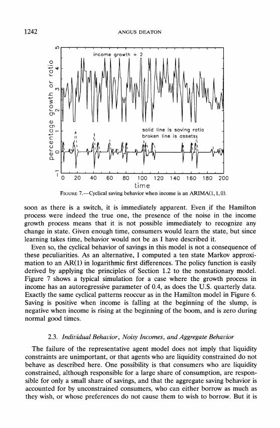
time FIGURE 7.-Cyclical saving behavior when income is an ARIMA(1, 1, 0).

soon as there is a switch, it is immediately apparent. Even if the Hamilton process were indeed the true one, the presence of the noise in the income growth process means that it is not possible immediately to recognize any change in state. Given enough time, consumers would learn the state, but since learning takes time, behavior would not be as I have described it.

Even so, the cyclical behavior of savings in this model is not a consequence of these peculiarities. As an alternative, I computed a ten state Markov approximation to an AR(1) in logarithmic first differences. The policy function is easily derived by applying the principles of Section 1.2 to the nonstationary model. Figure 7 shows a typical simulation for a case where the growth process in income has an autoregressive parameter of 0.4, as does the U.S. quarterly data. Exactly the same cyclical patterns reoccur as in the Hamilton model in Figure 6. Saving is positive when income is falling at the beginning of the slump, is negative when income is rising at the beginning of the boom, and is zero during normal good times.

2.3. Individual Behavior, Noisy Incomes, and Aggregate Behavior

The failure of the representative agent model does not imply that liquidity constraints are unimportant, or that agents who are liquidity constrained do not behave as described here. One possibility is that consumers who are liquidity constrained, although responsible for a large share of consumption, are responsible for only a small share of savings, and that the aggregate saving behavior is accounted for by unconstrained consumers, who can either borrow as much as they wish, or whose preferences do not cause them to wish to borrow. But it is


unlikely that income processes at the micro level exactly mirror the time-series behavior of aggregate income, so that an alternative approach is to work from the bottom up, starting not from the aggregate time-series process, but from those observed in the micro data. The final model that I examine represents an attempt to do so.

At the micro level, individual incomes are a good deal less persistent than is the case for the aggregate. Year to year changes show significant negative autocorrelation, either because there is substantial transitory income in each year, or because there is considerable measurement error in the data. The process I shall examine here is one in which, at the micro level, the first difference of logarithms has a moving average representation, i.e.

(32) Alny,-1a=

E-III-1,

where Et is a white noise process and 1 > qi > 0 is the moving average parameter. MaCurdy (1982) uses the PSID to estimate a model of this form for individual earnings, and although it is not his preferred model which is an MA(2), it fits the data almost as well. The representation (32) is equivalent to (log) income being the sum of white noise, (multiplicative) transitory income, and a random walk with drift, permanent income. In this interpretation, the parameter qi is 1 + [0 - (02 + 40)o.5]/2, where 0 is the ratio of the variance of the permanent component to the transitory component. MaCurdy's estimate for qi of 0.44 corresponds to value of 0 of 0.85, so that the permanent component accounts for just less than half the total variance in income.

Again, I assume a normal distribution for E, and again use an m-point approximation to simplify the computations. If the m states are labelled i = 1,... , m, there are m price functions p(w, i) defined by the functional equations,

(33) p(w,i) =max[A(w), E7njYJP

Xp([1 +iJ1(+r)(w-A-1P(wli))], I

where Yij = exp ( - - ei + 'iei) and rri is the probability that ei occurs, equal to 1/m here. I calculated (33) using MaCurdy's estimate of if = 0.44, growth rates of 0 and 2% per annum, and with r = 2%, U = 5%, and p = 2. MaCurdy estimates o, the standard deviation of e, the innovation to the logarithmic income process, to be 0.235, an enormous figure that would give a standard deviation for A ln yt of 0.25. If this estimate were correct, borrowing constraints would be unlikely to be a problem for most American earners. With earnings so uncertain, precautionary motives would tend to increase the desired growth rate of consumption and generate a great'deal of saving early in the life-cycle. In this sort of situation people are unlikely to wish to borrow; severe uncertainty and

1244 ANGUS DEATON

prudent preferences produce behavior that can look similar to that produced by liquidity constraints; see the excellent discussion in Zeldes (1986).

My presumption is that MaCurdy's estimate is too high because of the presence of substantial measurement error in recorded income, and I have experimented instead with values of oa of 0.10 and 0.15, themselves representing very substantial uncertainty in the income growth process. Logically, a reduction in oa should be accompanied by a decrease in qi, in order to accommodate the larger role of the permanent component. But the latter is already accounting for half of the variance in individual incomes, and a larger figure seems implausible.

The results are a hybrid between those where income is i.i.d. stationary and those where the growth process is positively autoregressive. The consumption functions have the usual general shape, but the low values of the innovations E correspond to the high branches of the consumption function. A high innovation now implies low income growth next period (because there is transitory noise in the income level), and so there will be a lower consumption ratio at the same cash on hand ratio when transitory income is high. This is the standard traditional explanation of procyclical savings out of transitory income. At the same time, high levels of current income growth reduce the cash on hand ratio, and also tend to reduce the consumption ratio. The net result is that, for example, with o= 0.15 and income growing at 2%, the regression of the consumption ratio on income growth has a coefficient around -0.2, so that the savings rate is procyclical. As a consequence, consumption is again smoother than income, with the standard deviation of consumption growth 0.13 as opposed to 0.17 for income growth. The liquidity constraints also generate a negative correlation between the consumption growth and lagged income growth. Such a correlation was found in the PSID data by Hall and Mishkin (1982), and was attributed by them to the presence of a fraction of liquidity constrained consumers spending their incomes. The explanation here runs somewhat dif- ferently, but the underlying cause is the same. (Note however that recent work by Mariger and Shaw (1988) suggests that Hall and Mishkin's finding is a phenomenon of the early 1970's and does not appear in the more recent waves of the PSID. The correlation should not therefore be treated as a proven fact.)

Consider now the transition from the individual consumers to the aggregate. If each income process were independent, then there would be no variation in aggregate income growth rates, and the saving and dissaving activities of individuals would cancel out in the aggregate. Instead of this, consider a simple model in which each consumer receives the aggregate shock together with idiosyncratic components. For each consumer, the growth rate of income is given by the following:

(34) Aln yt-g=Zlt +Z2t +Z3ts

ZTt =gro th +copt, 1 Z2to=g2the Z3t = 3t h r3t - 1

The first growth component, zl, together with the growth rate g, is common to


all consumers, and is assumed to be an MA(1) with positive parameter f3. Since both other components are taken to be idiosyncratic and independent over individuals, aggregate income growth will be z1 + g. (I assume for convenience that all income shares are the same, so average growth rates can be computed by simple averaging.) It would be more in accord with the aggregate data for the first component to be an AR(1) rather than an MA(1), but the former would much complicate the calculations to follow. The component Z2 is the innovation in an idiosyncratic random walk. Some such term must be present in order to match the large permanent component in individual income shocks, a role which cannot be played by the common shock because aggregate income growth is not sufficiently variable. The third component Z3 is the first difference of transitory income. Total income for each individual is the sum of a common IMA(1, 1), an idiosyncratic random walk, and transitory white noise.

The individual has no way of separating the three components, and observes only their sum, which is itself an IMA(1, 1) satisfying (32). I am thereby effectively assuming that consumers do not observe the aggregate shock, even with a lag. Clearly, such information is in fact available, but I assume either that consumers (irrationally) ignore it, or that, because it accounts for so little of individual income variance (see below), it is not worth consumers' time to discover it.

Matching (34) to both the aggregate data and the micro data ties down the parameters. From my interpretation of the micro data I take f = 0.44 and

= 0.15 as above. For the macro data, I take g = 0.02 and o1, the standard deviation of el, in (33), to be 0.01. A value of E of 0.5 generates an autocorrelation coefficient of 0.4 in the growth rates of income, in accord with the actually estimated AR(1). The other parameters can be calculated by matching the variances and covariances of Et - i/w-1 and z1 + Z2 + z3. After some rearrange- ment, this gives

(35) 22 = (1 - -)2 2-(1 + f)2 2

or32 = qlor2 + 'BU2

Note that because the innovation variance in the microeconomic growth process, so2, iS SO much larger than that in the aggregate, l2, the two idiosyncratic processes have to account for nearly all of the variance in individual income growth, something that matches the evidence that aggregate shocks have little explanatory power in individual earnings regressions.

Given that the parameters have been appropriately set, I can use the individual consumption functions previously calculated, simulate histories for a number of individuals, and do the aggregation explicitly. A simulated aggregate process z1 + g is generated first, and then this is added to individual independent z2 and Z3 processes for H consumers. The sum is then used to calculate consumption ratios according to the consumption functions in (33), and the process iterated forward. There is one minor complication in that the consump-

1246 ANGUS DEATON

tion functions A - 1{p(w, i)} from (33) are indexed on i, which is the element of the discrete approximation corresponding to the current innovation in the combined process, an innovation that bears no simple relationship to any of the innovations in (34). However, the moving average process (32) is invertible, and so its innovation can be recovered from the sum E:if'(A ln y,-i - g). Of course, this calculation will not yield a value that is one of the 10 points for which consumption functions have been calculated. For the moment, I have adopted the crude device of using the element of the approximation that is closest to the calculated innovation. Interpolation would be better, but since I am averaging over many consumers, it is hard to believe that the approximation errors are important in the aggregate.

Since individual income growth is negatively correlated, and aggregate income growth positively correlated, it is necessary to aggregate over a large number of households to eliminate the negative effects. In practice, 1000 cases seemed to be adequate, and yielded, over 200 periods, an aggregate income change with a sample mean of 0.0192 and standard deviation of 0.0125, compared with the theoretical magnitudes for infinite H of 0.02 and 0.0125 respectively. The sample autocorrelation coefficient of A ln y is 0.262, well below the theoretical value of 0.40. The aggregate consumption ratio (i.e. the simple average of the 1000 individual ratios) responds to income growth with a coefficient of -0.17, so that, while savings ratios are procyclical, the effects are small. It would take a 2.4 standard deviation increase in the income growth rate to shift the saving rate up by half a percentage point. As a result, while consumption is smoother than income, with a standard deviation of A ln c of 0.0114 as opposed to 0.0125 for income growth, the smoothing effect is very small. Assets are now always positive, although for each individual, assets are frequently zero. As a consequence, capital income allows the consumption ratio to average a little more than unity, 1.0015 in the simulations reported here. The growth rate of aggregate consumption has a positive regression coefficient (0.42) on lagged aggregate income growth, as opposed to the negative coefficient in the micro data. The model therefore provides a means of reconciling the actual (or at least possible) orthogonality condition failures in the micro data (Hall and Mishkin) with those in the macro data (Flavin), which also display the negative/positive pattern.

These results show that the model of this section is capable of providing a coherent account of a number of disparate phenomena in both microeconomic and macroeconomic data. However, it is important to note that the story is still incomplete in a number of important respects. While I believe that understand- ing the behavior of liquidity constrained consumers is important, I would not wish to claim that all consumers are in this position. There are relatively patient individuals as well as impatient ones, and the former are likely to accumulate considerable amounts of wealth in the standard life-cycle manner. I suspect that such people are in the minority, although they account for a disproportionate share of aggregate saving and wealth accumulation. Finally, while it is true that most Americans accumulate very few financial assets, they do accumulate


housing wealth and pension rights. Some of this saving is involuntary, but a fuller account would integrate the existence of these other assets into the models developed in this paper.

Research Program in Development Studies, Princeton University, Princeton, N.J. 08544, U.S.A.

Manuscript received December, 1989; final revision received October, 1990.

REFERENCES

ALTONJI, J. G., AND A. Siow (1987): "Testing the Response of Consumption to Income Change with (Noisy) Panel Data," Quarterly Journal of Economics, 102, 293-328.

BARSKY, R. B., N. G. MANKIW, AND S. P. ZELDES (1986): "Ricardian Consumers With Keynesian Propensities," American Economic Review, 76, 676-691.

BEWLEY, T. (1977): "The Permanent Income Hypothesis: A Theoretical Formulation," Journal of Economic Theory, 16, 252-292.

CAMPBELL, J. Y. (1987): "Does Saving Anticipate Declining Labor Income? An Alternative Test of the Permanent Income Hypothesis," Econometrica, 55, 1249-1274.

CARROLL, C., AND L. H. SUMMERS (1989): "Consumption Growth Parallels Income Growth: Some New Evidence," Department of Economics, Massachusetts Institute of Technology and Harvard University.

DEATON, A. S. (1990): "Saving in Developing Countries: Theory and Review," World Bank Economic Review, Special Issue, Proceedings of the Annual World Bank Conference on Develop- ment Economics.

DEATON, A. S., AND G. LAROQUE (FORTHCOMING): "On the Behavior of Commodity Prices," Review of Economic Studies, forthcoming.

FLAVIN, M. (1981): "The Adjustment of Consumption to Changing Expectations about Future Income," Journal of Political Economy, 89, 974-1009.

FOLEY, D., AND M. HELLWIG (1975): "Asset Management with Trading Uncertainty," Review of Economic Studies, 42, 327-346.

HALL, R. E., AND F. S. MISHKIN (1982): "The Sensitivity of Consumption to Transitory Income: Estimates from Panel Data on Households," Econometrica, 50, 461-481.

HAMILTON, J. D. (1989): "A New Approach to the Economic Analysis of Nonstationary Time Series and the Business Cycle," Econometrica, 57, 357-384.

HELLER, W. P., AND R. M. STARR (1979): "Capital Market Imperfection, the Consumption Function, and the Effectiveness of Fiscal Policy," Quarterly Journal of Economics, 93, 455-463.

HELPMAN, E. (1981): "Optimal Spending and Money Holdings in the Presence of Liquidity Constraints," Econometrica, 49, 1559-1570.

IMROHOROGLU, A. (1989): "Cost of Business Cycles with Indivisibilities and Liquidity Constraints," Journal of Political Economy, 97, 1364-1383.

KIMBALL, M. S. (1990): "Precautionary Saving in the Small and in the Large," Econometrica, 58, 53-73.

KOTLIKOFF, L. J., AND L. H. SUMMERS (1981): "The Role of Intergenerational Transfers in Aggregate Capital Accumulation," Journal of Political Economy, 89, 706-732.

LEVHARI, D., L. J. MIRMAN, AND I. ZILCHA (1980): "Capital Accumulation under Uncertainty," International Economic Review, 21, 661-671.

MACURDY, T. E. (1982): "The Use of Time Series Processes to Model the Error Structure of Earnings in Longitudinal Data Analysis," Journal of Econometrics, 18, 83-114.

MARIGER, R., AND K. SHAw (1988): "Unanticipated Aggregate Disturbances and Tests of the Life-Cycle Consumption Model Using Panel Data," Department of Economics, University of Washington, Seattle.

MENDELSON, H., AND Y. AMIHUD (1982): "Optimal Consumption Policy Under Uncertain Income," Management Science, 28, 683-697.

1248 ANGUS DEATON

SCHECHTMAN, J. (1976): "An Income Fluctuation Problem," Journal of Economic Theory, 12, 218-241.

SCHECHTMAN, J., AND V. ESCUDERO (1977): "Some Results on 'An Income Fluctuation Problem'," Journal of Economic Theory, 16, 151-166.

SKINNER, J. (1988): "Risky Income, Life-Cycle Consumption, and Precautionary Savings," Journal of Monetary Economics, 22, 237-255.

TAUCHEN, G. (1986): "Finite State Markov Chain Approximations to Univariate and Vector Autoregressions," Economics Letters, 20, 177-181.

ZELDES, S. (1986): "Optimal Consumption With Stochastic Income: Deviations from Certainty Equivalence," Wharton School, University of Pennsylvania.

(1989a): "Consumption and Liquidity Constraints: An Empirical Investigation," Journal of Political Economy, 97, 305-346.

(1989b): "Optimal Consumption With Stochastic Income: Deviations from Certainty Equiva- lence," Quarterly Journal of Economics, 104, 275-298.

Documents

BY - Princeton Universitydeaton/downloads/Saving_and_Liquidity... · Limited borrowing opportunities may also help to explain the observed ... but cannot do so typically can do