Embed Size (px)
Citation preview

THE SPATIO-TEMPORAL EVOLUTION OF IRRIGATION IN THE GEORGIA COASTAL
PLAIN: EMPIRICAL AND MODELED EFFECTS ON THE HYDROCLIMATE
by
Marcus De’Andre Williams
(Under the Direction of J. Marshall Shepherd)
ABSTRACT
Agricultural landscapes comprise up to 40% of global land cover and population growth
increases the need to grow current levels of agriculture. Irrigated agriculture increased globally
during the last century as a result of improved technology. The impacts of this rapid expansion
have been the focal point of many studies, but very few have focused on the southeastern United
States. Irrigation impacts the hydrologic cycle and surface energy budget through increased
evapotranspiration as a result of increased surface moisture. Georgia has experienced rapid
growth in irrigated area since the early 1970s with most irrigated lands being converted from
previously un-irrigated agriculture. The overarching goal of this research addresses irrigation-
hydroclimate relationships in the southeastern United States, with a primary focus on southwest
Georgia. While there is regional dependence on the beneficial effects of increased irrigation to
improve agricultural yield, there is limited refereed literature on the influence of expansion of
irrigation on Georgia’s climate. The analysis conducted uses remote sensing and geographic
information system (GIS) technologies to quantify past and current spatio-temporal trends in
irrigated acreage in Georgia. The identification of these trends allows for the assessment of the

impacts of irrigation on local to regional hydroclimate through observation and modeling
analysis.
INDEX WORDS: Irrigation, Remote Sensing, Regional Climate Change, Climate Modeling

THE SPATIO-TEMPORAL EVOLUTION OF IRRIGATION IN THE GEORGIA COASTAL
PLAIN: EMPIRICAL AND MODELED EFFECTS ON THE HYDROCLIMATE
by
Marcus De’Andre Williams
B.S. Florida State University, 2006
M.S., Florida State University, 2010
A Dissertation Submitted to the Graduate Faculty of The University of Georgia in Partial
Fulfillment of the Requirements for the Degree
DOCTOR OF PHILOSOPHY
ATHENS, GEORGIA
2016

©2016
Marcus De’Andre Williams
All Rights Reserved

THE SPATIO-TEMPORAL EVOLUTION OF IRRIGATION IN THE GEORGIA COASTAL
PLAIN: EMPIRICAL AND MODELED EFFECTS ON THE HYDROCLIMATE
by
Marcus De’Andre Williams
Major Professor: J. Marshall Shepherd
Committee: Andrew J. Grundstein
Marguerite Madden
Alan P. Covich
Electronic Version Approved:
Suzanne Barbour
Dean of the Graduate School
The University of Georgia
August 2016

DEDICATION
This dissertation is dedicated to my family. They provided me with the inspiration to
keep pressing forward and provided vital support to me throughout this journey. None of this
would be possible without them. I would also like to thank all of the special educators who
fostered my desire to learn. I also dedicate this work to my friends who have been there with me
through my early childhood and who are like brothers to me. I want to especially acknowledge
my wife and daughter, who are my backbone and inspiration for all my current and future
achievements.
iv

ACKNOWLEDGMENTS
I would like to thank Dr. J. Marshall Shepherd for being a mentor in my academic career
and personally. I cannot think of a better mentor to learn from as an early career scientist. It is an
honor to work with someone as distinguished, and famous. I would also like to thank my
committee, Drs. Andrew Grundstein, Marguerite Madden, and Alan Covich for their feedback
and guidance during the process. I would also like to Dr. Scott Goodrick and my colleagues at
the United States Forest Service for their support and insight.
v

Table of Contents
ACKNOWLEDGMENTS .............................................................................................................. v
1) INTRODUCTION AND LITERATURE REVIEW .............................................................. 1
1.1 Introduction and Literature Review ................................................................................. 1
1.2 Research Objectives ......................................................................................................... 6
1.3 Summary .......................................................................................................................... 9
2) MAPPING THE SPATIO-TEMPORAL EVOLUTION OF IRRIGATION IN THE
COASTAL PLAIN OF GEORGIA, USA .................................................................................... 18
Abstract ................................................................................................................................. 18
2.1 Introduction .................................................................................................................... 19
2.2 Literature Review ........................................................................................................... 21
2.3 Study Area, Data, and Methods ..................................................................................... 23
Study Area ............................................................................................................................ 23
Data and Methods ................................................................................................................. 24
2.4 Results ............................................................................................................................ 29
2.5 Discussion ...................................................................................................................... 33
2.6 Conclusion ...................................................................................................................... 36
2.7 References ...................................................................................................................... 38
vi

3) COMPARISON OF DEW POINT TEMPERATURE ESTIMATION METHODS IN
SOUTHWESTERN GEORGIA ................................................................................................... 54
Abstract ................................................................................................................................. 55
3.1 Introduction and Literature Review ............................................................................... 56
3.2 Data and Methodology ................................................................................................... 59
Data ....................................................................................................................................... 59
Linear Regression ................................................................................................................. 59
Artificial Neural Network ..................................................................................................... 61
3.3 Results and Discussion ................................................................................................... 62
Linear Regression ................................................................................................................. 62
3.4 Conclusion ...................................................................................................................... 66
3.5 References ...................................................................................................................... 67
4) INTEREPOCHAL CHANGES IN TEMPERATURE, HUMIDITY, AND
PRECIPITATION ASSOCIATED WITH INCREASING IRRIGATION IN THE GEORGIA
COASTAL PLAIN ....................................................................................................................... 81
Abstract ................................................................................................................................. 81
4.1 Introduction and Literature Review ............................................................................... 82
4.2 Data and Methods........................................................................................................... 84
4.3 Results ............................................................................................................................ 86
vii

Temperature .......................................................................................................................... 86
Precipitation .......................................................................................................................... 89
4.4 Discussion ...................................................................................................................... 90
4.5 Conclusion ...................................................................................................................... 93
4.6 References ...................................................................................................................... 94
5) ON THE IMPACT OF IRRIGATION ON SUMMERTIME SURFACE FLUXES AND
PRECIPITATION IN SOUTHWEST GEORGIA: A MODEL SENSITIVITY APPROACH . 114
Abstract ............................................................................................................................... 114
5.1 Introduction and Literature Review ............................................................................. 115
5.2 Methodology ................................................................................................................ 117
WRF and Model Configuration .......................................................................................... 118
5.3 Results and Analyses .................................................................................................... 120
Sensible and Latent Heat Flux ............................................................................................ 120
Precipitation ........................................................................................................................ 122
5.4 Summary ...................................................................................................................... 123
5.5 References .................................................................................................................... 124
6) SUMMARY AND CONCLUSIONS ................................................................................. 140
6.1 Overview ...................................................................................................................... 140
viii

6.2 Conclusions .................................................................................................................. 141
Table 2-1: Table providing information on the Landsat missions used in analysis...................... 44
Table 3-1 Error and model evaluation statistics of Equation 1 for the individual stations. The
coefficients for the regression equation are derived from a merged data set containing data from
all seven stations listed below. The model evaluation parameters are root mean square error
(RSME), mean absolute error (MAE), Pearson’s correlation coefficient (R), index of agreement
(D) and the coefficient of efficiency (E). ...................................................................................... 77
Table 3-2 Same as Table 1, except for Equation 2. ...................................................................... 78
Table 3-3 Same as Table 1, except for Equation 3. ...................................................................... 78
Table 3-4 Error and model evaluation statistics for the independent stations using Equation 3. . 79
Table 3-5 Error and model evaluation for Arlington during the growing season, daily
precipitation, and three day precipitation using H03 Method 4.................................................... 79
Table 3-6 Error and model evaluation statistics of the ANN for the individual stations. ............. 79
Table 3-7 Same as table 6, except for independent stations. ........................................................ 80
Table 3-8 Comparison of RMSE and MAE for Equation 3 and the ANN for the independent
stations. ......................................................................................................................................... 80
Table 5-1: 24-class land use classification used in the WRF simulations derived from USGS. 130
Table 5-2: Table showing land surface parameters for the NO-IRR and IRR model simulations.
..................................................................................................................................................... 133
ix

Figure 1.1: USDA map of irrigated land in 2012. Red box highlights the study area (USDA
Census of Agriculture, 2012) ........................................................................................................ 11
Figure 1.2: Time series of average number of farms (blue) and average farm size (red) from 2008
- 2015. Figure credit Mayo, 2016 ................................................................................................. 12
Figure 1.3: Depiction of the Hydrologic cycle. Red arrows and circles denote the impact of
irrigation on the water cycle (The Water Cycle USGS, 2016). .................................................... 13
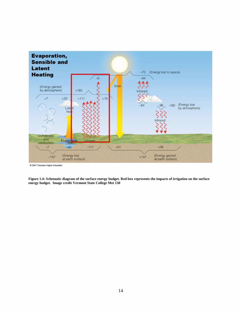
Figure 1.4: Schematic diagram of the surface energy budget. Red box represents the impacts of
irrigation on the surface energy budget. Image credit Vermont State College Met 130 ............. 14
Figure 1.5: Farm sales for 2012. Shaded colors represent the percentage of farms per county with
sales greater than $250, 000. Black box highlights area of interest in this study (USDA Ag
Census, 2012) ................................................................................................................................ 15
Figure 1.6: Diagram of water withdrawals between the public supply, industrial, and agricultural
irrigation sectors in the Apalachicola-Chattahoochee-Flint Basin (Maella, 1990). ...................... 16
Figure 1.7: Google Earth image of southwest Georgia. Red box highlights a portion of the study
area. Circular areas in image are center pivot irrigation systems. The strip of panchromatic
imagery in the center a result of images from other sources being combined. ............................. 17
Figure 2.1: Physiographic provinces of Georgia .......................................................................... 45
x

Figure 2.2: Natural, False, and Brightness, Wetness and Greenness (BWG) tasseled cap
composites of Miller Country, Georgia, USA .............................................................................. 46
Figure 2.3: Total center pivot systems and acreage irrigated (hectares) ....................................... 46
Figure 2.4: Percent change in center pivot irrigation systems (blue) and total acreage (red). ...... 47
Figure 2.5: Map of 1976 CPI systems overlaid on a Landsat false color composite. The variations
in the hue are due to the composite pulling from scenes from different dates. ............................ 48
Figure 2.6: Map of 1996 CPI systems overlaid on a Landsat composite of tasseled cap indices. 49
Figure 2.7: Map of 2013 CPI systems overlaid on Landsat false color composite. ..................... 50
Figure 2.8 County breakdown of total hectares irrigated for 2013 ............................................... 51
Figure 2.9 County breakdown of percent of total land area irrigated for 2013 ............................ 52
Figure 2.10 Map of NAIP imagery compared to a Landsat scene. ............................................... 53
Figure 3.1 Map of stations used in development of the regression models (blue) and testing of the
regression models (red) ................................................................................................................. 72
Figure 3.2 Basic network design of the ANN. This ANN is a feed-forward multilayer perceptron
with one hidden layer using sigmoid activation functions and trained using back-propagation.
The ANN consists of an input layer, a hidden layer, and an output layer. ................................... 73
Figure 3.3(a) Time series of observed and estimated dew point temperatures of H03 Equation 3
for Arlington automated weather station. The black line represents observed values and the grey
line represents the estimated values. The x-axis represents the date and the y-axis represents
temperature in degrees Celsius. (b) Observed versus Estimated scatter plot for Arlington
GEAMN station. The x-axis and y-axis are shown in degrees Celsius. ....................................... 74
xi

Figure 3.4 Performance of Equation 3 for the Arlington automated weather station. The x-axis
represents the absolute error in degrees and the y-axis represents the percent of cases associated
with the corresponding error. ........................................................................................................ 75
Figure 3.5 Performance comparison of various neural network architectures for dew point
estimation. Network architectures are given on x axis and are defined by the number of input and
hidden nodes: 3_2 represents a network with 3 inputs and 2 hidden nodes. ................................ 76
Figure 3.6 Performance of the ANN represented as a percentage for varying dew point
temperature ranges. The x-axis represents the absolute error in degrees and the y-axis represents
the percent of cases for the given absolute error. .......................................................................... 77
Figure 4.1: 2012 Irrigated acres in the United States. Photo credit to USDA Census of
Agriculture .................................................................................................................................... 99
Figure 4.2: Map of 19 NWS Coop stations used in analysis ...................................................... 100
Figure 4.3: Pre and Post Irrigation minimum temperature difference graph. Calculated by
subtracting post irrigation average from pre irrigation average. Averages for all 19 stations
shown. ......................................................................................................................................... 101
Figure 4.4: Pre and Post Irrigation minimum temperature difference maps. Green denotes
stations that had significant increases in June, July, and August minimum temperatures during
the post irrigation epoch. Red denotes averages for the 13 remaining stations .......................... 102
Figure 4.5: Pre and post irrigation dew point temperatures for all 19 stations ........................... 103
Figure 4.6: Pre and Post Irrigation dew point temperature difference maps. Green denotes
stations that had significant increases in June, July, and August dew point temperatures during
the post irrigation epoch. Red denotes averages for the 13 remaining stations .......................... 104
xii

Figure 4.7: Pre and post irrigation maximum temperature difference for all 19 stations. .......... 105
Figure 4.8: Pre and post irrigation precipitation difference for all 19 stations. .......................... 106
Figure 4.9: Map showing location of Albany NWS Coop station (green circle). The red circles
represent mapped center pivot irrigation (CPI) systems for 2008. ............................................. 107
Figure 4.10: Albany, GA pre and post irrigation difference graphs for precipitation (upper left),
minimum temperature (upper right), maximum temperature (lower left), and dew point
temperatures (lower right). Blue represents the pre-irrigation averages minus the 1938-2013
period of record (P.O.R.). Red represents post irrigation minus P.O.R. and green represents post
irrigation minus pre irrigation values. ......................................................................................... 108
Figure 4.11: Map showing location of Camilla NWS Coop station (green circle). The red circles
represent mapped center pivot irrigation (CPI) systems for 2008. ............................................. 109
Figure 4.12: Camilla, GA pre and post irrigation difference graphs for precipitation (upper left),
minimum temperature (upper right), maximum temperature (lower left), and dew point
temperatures (lower right). Blue represents the pre-irrigation averages minus the 1938-2013
period of record (P.O.R.). Red represents post irrigation minus P.O.R. and green represents post
irrigation minus pre irrigation values .......................................................................................... 110
Figure 4.13: Map of HYSPLIT back trajectory calculations for Alma, GA. Black and blue
asterisks represent trajectory calculations for July 1st and 2nd respectively. Red represents the
mapped CPI systems in 2008. ..................................................................................................... 111
Figure 4.14: Wind Rose diagram for Alma, GA ......................................................................... 112
Figure 4.15: Map showing location of Colquitt NWS Coop station (green circle). The red circles
represent mapped center pivot irrigation (CPI) systems for 2008. ............................................. 113
xiii

Figure 5.1: Depiction of the water cycle and alterations caused by irrigation. Image obtained
from the United States Geological Survey.................................................................................. 128
Figure 5.2: Depiction of the surface energy budget and the modifications caused by irrigation.
Image courtesy of Lyndon State University department of Meteorology. ................................. 129
Figure 5.3: Land use category for NO-IRR model simulations. ................................................. 131
Figure 5.4: Land use category for IRR model simulations. ........................................................ 132
Figure 5.5: Image of model domain set up. Largest domain D1 has a horizontal resolution of
15km, medium domain D2 has a horizontal resolution of 5km, and innermost domain D3 has a
horizontal resolution of 1km. ...................................................................................................... 133
Figure 5.6: June 30th sensible heat flux for a) NO-IRR, b) IRR, and c) the differences in sensible
heat flux between the two simulations. ....................................................................................... 134
Figure 5.7: Sensible and Latent heat flux for NO-IRR and IRR simulations. Plots are for grid
point near 31.5N and -83.5W (Coffee County). Blue and yellow lines represent NO-IRR latent
and sensible heat fluxes respectively. Red and grey lines represent IRR latent and sensible heat
fluxes, respectively. .................................................................................................................... 134
Figure 5.8: 20z June 30 sensible heat flux for a) NO-IRR, b) IRR, and c) the difference in flux
between the two surfaces. ........................................................................................................... 135
Figure 5.9: 18z July 11th differences in latent heat flux between NO-IRR and IRR simulations
(W/m2)......................................................................................................................................... 135
Figure 5.10: Sensible heat flux for 18z July 18th 2014 (W/m2). ................................................ 136
xiv

Figure 5.11: Image showing observed 24-hr precipitation on left hand side and model
accumulated precipitation on June 30th, 2014. Obeserved precipitation photo credit to NCEP
(http://www.wpc.ncep.noaa.gov/dailywxmap/index_20140630.html) ....................................... 137
Figure 5.12: Total simulation precipitation difference map for NO-IRR and IRR June 29ht-30th
simulation. ................................................................................................................................... 138
Figure 5.13: Total simulation precipitation difference map for NO-IRR and IRR July 10th-11th
simulation. ................................................................................................................................... 139
xv

1
1) INTRODUCTION AND LITERATURE REVIEW
1.1 Introduction and Literature Review
Agricultural production is a critical part of sustaining human life on earth. During a period
known as the “Green Revolution”, agricultural productivity doubled to meet rising demands of a
growing population (Tilman, 1999). With an expected global population of 11.2 billion by the
year 2100 (United Nations, 2015), the current levels of agricultural intensity are expected to
increase to support future food demands of the population. Historically, agricultural landscapes
relied on natural methods for irrigation, but more recently there has been rapid growth towards
artificially irrigated landscapes. The United States Geological Survey (USGS) defines irrigation
as “the controlled application of water for agricultural purposes through man-made systems to
supply water requirements not satisfied by rainfall (USGS, 2016). Irrigation has rapidly
expanded around the globe and can be a strain on already limited water resources. The global
area equipped for irrigation was estimated to be 324 million hectares in the year 2012, with
approximately 26.4 million hectares equipped for irrigation in the United States (Figure 1.1)
(FAO, 2014). Growing population, decreases in the number of farms, and an overall increase in
the total number of farms (Figure 1.2) (Mayo, 2016) exacerbate the need for remaining farmland
to have optimal efficiency and productivity. It is postulated that the above changes increase the
need for efficient irrigation as the average value of production was more than three times greater
for irrigated farmland than for dryland farmland (Schaible and Aillery, 2012). From a water use
standpoint, irrigation accounts for 80-90 percent of the United States’ consumptive water use and
much of the irrigated water is lost to atmosphere through evapotranspiration (USDA, 2012). The

2
bulk of this water is supplied by groundwater (38 percent global and nearly half in the United
States) and is in contention with municipal water use and thermoelectric power (USDA, 2012).
Irrigation is an anthropogenic disturbance of the land surface; much like urbanization
which is a widely known climate forcing that alters temperature and precipitation patterns
(Mahmood et al., 2010). The literature is conclusive that irrigation significantly modifies the land
surface, and it affects surface energy budgets, the water cycle, and climate (Cook et al., 2014).
Figure 1.3 (Hydrologic cycle) illustrates the various aspects of the hydrologic cycle that
irrigation modifies. Those branches of the hydrologic cycle affected by irrigation include
precipitation, water storage in the atmosphere via increased evaporation, and ground water
storage. Irrigation alters the surface energy budget (Figure 1.4) by modifying evaporation,
convection, latent and sensible heat fluxes, cloud coverage, and potentially soil-heat fluxes. One
common theme in irrigated areas that impacts both the local hydrologic cycle and the surface
energy budget is the increase in near surface moisture. This increased moisture extending into
the lower levels of the atmosphere has the ability to modify existing land-atmosphere
interactions which are a critical driver of earth’s climate system over continental scales (Pei et al,
2016). This modification takes place primarily through partitioning incoming solar radiation
towards increased latent heating. The increase in latent heating results in decreased sensible
heating that modifies temperature and evapotranspiration rates due to changes in the Bowen ratio
with the Bowen ratio defined as the ratio of sensible heat flux to latent heat flux. The increased
amount of near surface moisture can potentially modify existing precipitation patterns (Barnston
and Schickedanz 1984, DeAnglis et al., 2010). These impacts begin at the local scale

3
approximately 0.5 to 5 km in size and can extend to the regional scales of 100 to 10,000 km ,
although the effects of irrigation on regional climate are less certain and are often region specific
(Pei et al, 2016). Therefore, there is a critical need to quantify the extent of irrigated areas in
order to identify what areas are impacted and to what extent. It has been postulated that increased
irrigation has led to a local, and in some cases regional, cooling trend in maximum and minimum
temperatures, as well as diurnal temperature range (DTR) (Greets 2002, Lobell and Bonfils 2008,
Kueppers 2007, Snyder and Sloan 2007). DeAngelis et al. (2010) noted that precipitation
increased by15-30% downwind of heavily irrigated areas near the Ogallala aquifer, which is part
of the High Plains Aquifer System. Many of the aforementioned studies were conducted for
semi-arid regions that are believed to have a heavy reliance on irrigation. However, the
uncertainty of future climate change and drought frequency may lead the southeastern United
States (SE US) to rely on irrigation in the same manner as the semi-arid regions. To summarize
the known impacts of irrigation, literature has shown that irrigation reduces maximum
temperatures, increases minimum temperatures, enhances precipitation downwind of irrigated
areas, and increases low level moisture (Adegoke 2003, Barnston and Schickedanz 1984,
Boucher 2004, Marshall and Pielke 2004, Sen Roy et al. 2007).
There have been efforts to map irrigated areas globally as well as in the United States and
separate studies attempt to quantify the impacts of irrigation on climate. The analysis conducted
here synthesizes these often separate investigations into one comprehensive study. The primary
area of focus of this dissertation research is the Georgia Coastal Plain (Figure 1.1), covering an
area of approximately 92, 333 km2. The Georgia Coastal Plain landscape is characterized by
4
relatively gently rolling to level topography with elevations ranging from approximately 228
meters to sea level. At higher elevations, there is little level terrain except for the occasion
marshy flood plain or narrow steam terrace. Soils are generally productive, well-drained, and
moderately permeable. However, in areas of nearly level terrain, i.e., closer to the coast of
Georgia, the soils become restrictive for agriculture and pasture (Hodler and Schretter, 1986).
The 1,267 mm of annual rainfall that Georgia receives is enough to support the agriculture in the
state, but the varying nature of the spatial distribution of this rainfall along with increases in
drought frequency has increased the need for irrigation to support agricultural crop growth.
Agriculture is the largest industry in Georgia and contributed more than $72 billion to the
state’s economy in 2015 (Georgia Farm Bureau, 2016) with one out of every seven residents of
the state working in agriculture or forest related fields (UGA Cooperative Extension, 2011).
Southwest Georgia is responsible for a large percentage of Georgia’s agricultural production
(Figure. 1.5) and several of the counties in this area account for the highest agricultural water
withdrawals (Figure 1.6) (Lawrence, 2016). Much of the land cover in this region was converted
from un-irrigated agriculture to irrigated croplands during the early 1970s to 2008 (Martin et al.,
2013).
The primary focus of this research is to investigate the hypotheses that: (1) irrigation has
rapidly increased in Georgia, and (2) this rapid increase in irrigation has modified aspects of the
hydroclimate such as humidity, temperature, and precipitation in the region. One interesting
aspect that distinguishes this study from others is the lack of refereed literature stating the
impacts of irrigation on Georgia’s climate. The impact of irrigation has been investigated on

5
water resources, how climate change impacts irrigation demand, and impact on stream flows.
Misra et al 2012 is one of the few studies that quantified the climatic impact of irrigation on
Georgia’s climate, but their analysis was in conjunction with other states in the southeast United
States. Irrigation in Georgia has been classified as sporadic from a spatial density standpoint
(Pervez and Brown, 2010) and is often not considered as having an impact in global irrigation
studies. Irrigation water use is also an important issue in Georgia, as the state is in a legal dispute
with Alabama and Florida over downstream usage of water. This dispute is known as the “Tri-
State” water wars. The Flint river basin in Georgia has the highest amount of water use within
the state and is the upstream user of water that the Florida shellfish industry is reliant upon.
A more detailed discussion of the research objectives is presented later in this chapter, but
a brief summary is instructive here. This research addresses irrigation-hydroclimate relationships
in the southeastern United States, with a primary focus on southwest Georgia. The first objective
quantified the spatio-temporal evolution of irrigation in the Coastal Plain of Georgia. This was
assessed through mapping areas equipped for irrigation in the Georgia Coastal Plain aided by
Landsat satellite imagery (Figure 1.7). Building from the irrigation analysis, a simple method to
estimate daily dew point temperatures using temperature and precipitation observations was
developed. Chapter 2 describes the methodology and results. One of the climate system
responses to irrigation is increased low level moisture and the development of a dew point
estimation method allows for the capture of any long term changes in moisture content in the
region using dew point temperature as a proxy. With many long-term observations of dew point
6
temperature existing at first order stations, which do not share common characteristics of rural
and irrigated weather stations, this research objective addressed this issue.
The impact of irrigation on the hydro-climate was investigated by applying the daily dew
point temperature estimation method to existing National Weather Service (NWS) Cooperative
Observation Network (Coop) stations. Changes in temperature and precipitation were also
evaluated. The relative response of the hydro-climate to transitioning the land surface from dry
cropland, and then to an irrigated land cover was investigated using a numerical weather
modeling system called the Weather Research and Forecasting (WRF) Model.
1.2 Research Objectives
Understanding the influence of past land use changes on climate is needed to improve
regional projections of future climate change and inform debates about the tradeoffs associated
with land use decisions (Bonfils and Lobell, 2007). The rapid expansion of irrigated area in the
20th century has remained unclear relative to other land use changes (Kueppers et al 2007).
Changes in irrigation may also be expected to influence climate because soil moisture affects
surface albedo and evaporation and has been shown to influence regional temperature (Dai et al,
1999). Irrigated landscapes can alter the regional surface energy balance and its associated
temperature, humidity, and climate features (Sen Roy et al., 2007)
Chapter 2 identifies the spatio-temporal evolution of areas equipped for irrigation in the
Georgia Coastal Plain. Prior irrigation mapping studies (Doll and Siebert 1999, Ozdogan and
Gutman 2008, Siebert et al. 2005,) conducted at the global and national scale are done with very
7
coarse pixel size resolution (10-km to 500-m). Many of the studies produced maps that
represented irrigated areas as a percentage of the pixels unit area, which does not provide
information on the sub pixel location of irrigated areas. While this is sufficient for national and
global applications, this level of detail is not adequate for regional analysis. Boken et al. (2004)
stated that sub-county, high resolution irrigation mapping would lend better understanding to
agricultural water use. This chapter answers the following research questions:
• Has irrigation increased in the Georgia Coastal Plain?
• Over what time period has irrigation increased most significantly?
• Given the spatial area of interest, where is irrigation most intense?
Chapter 3 investigates a method to estimate dew point temperatures using readily
obtained daily temperature and precipitation observations. There is an absence of long term dew
point temperatures outside of first order observation stations. First order stations are weather
stations that are professionally maintained by the National Weather Service (NWS) or the
Federal Aviation Administration (FAA) (NWS, 1999). First-order observation stations are often
in areas that are not representative of agricultural areas, which created the need to develop a
simple method to estimate dew point temperature and provide a metric to estimate historical dew
point temperatures. Two methods of estimation were considered, a liner regression approach as
well as an automated neural network approach. The neural network approach performed better,
with minimum temperature, diurnal temperature range (difference between daily maximum and
minimum temperature), and daily precipitation as input variables. Daily dew point temperatures

8
that extended back as far as observations were available can now be calculated, as they could not
before this method was developed. Chapter 4 applies the daily dew point estimation method as
well as analyzing temperature and precipitation methods to assess irrigation-induced changes in
the region. Knowledge of the impacts of irrigation on climate is vital for understanding causes of
past climate change and to anticipate the direction and magnitude of future changes in
agricultural regions (Lobell and Bonfils, 2008). Chapters 3 and 4 together combine to answer the
following research questions
• Has irrigation impacted hydro-climatic variables in the region?
• What type of influence, if any, has irrigation produced on hydro-climatic variables in the
analysis region? Is the pre-irrigation climatology of the region different from the post-irrigation
climatology?
• From the perspective of the long-term spatio-temporal characteristics of the hydro-
climatic variables in the region; how are heavily irrigated surfaces different than non-irrigated
surfaces?
• What hydro-climatic variable(s) is (are) most influenced by irrigation?
The aim of Chapter 5 is to investigate if there are any relative differences in the sensible
and latent heat fluxes along with spatial differences in precipitation patterns between non-
irrigated and irrigated land surfaces. This analysis presented a theoretical approach to quantify
differences in hydro-climatic variables and their response to different land surfaces. Precipitation
impacts of irrigation are often region specific (Adegoke, 2008). Pie et al. (2016) showed that

9
excess moisture from irrigation is transported to Georgia, but there was no mention of how the
introduction of irrigation has modified the local and regional climate. The relationship is poorly
understood in the analysis region (Boken et al., 2004) and has minimal observational findings to
support how irrigation influences precipitation (Sen Roy et al. 2010). The proposed analysis here
is focused around the following questions;
• Can irrigation theoretically impact hydro-climatic variables in humid regions?
• Has irrigation influenced moisture and precipitation transport patterns in the region?
• Are there distinct contributions to moisture and precipitation transport between two
distinct representations of irrigated landscapes?
1.3 Summary
This dissertation addresses the need for a comprehensive understanding on how irrigation
has influenced climate in a humid environment. Most of the studies of this nature are conducted
for semiarid areas of the world because it is believed that areas with adequate rainfall do not?
rely on irrigation as much. With uncertainties in drought frequency and the potential impacts of
climate change, the humid Eastern United States has seen an upward trend in irrigation. This
dissertation, using remote sensing methods, quantifies the high temporal and spatial resolution of
the trends of irrigated areas in Georgia.
The lack of adequate long term meteorological observations in the region makes it difficult
to provide a purely empirical assessment of irrigation-induced modification of the climate. To
address this shortcoming, high-resolution modeling is employed to assess the relative impacts on

10
climate when a land surface transitions from unirrigated to irrigated agriculture. The overarching
goal of the following chapters is to answer some of the uncertainties associated with irrigation
and climate in the study area. This study will help to characterize the role of irrigation on hydro-
climatic variables in the Georgia Coastal Plain. Although extensive literature exists for
California and the Great Plains regions of the United States, a relative absence of any detailed
analysis investigating the impacts of irrigation on climate in the Southeastern United States, is
available. To date, this research is one of the few to create a mapped time series of irrigated area
for Georgia and one of the few to provide historical analysis of long term dew point temperature
trends outside of first order stations in Georgia. This research will also provide context for the
impacts of irrigation in climates that are not moisture limited.

11
Figure 1.1: USDA map of irrigated land in 2012. Red box highlights the study area (USDA Census of Agriculture, 2012)

12
Figure 1.2: Time series of average number of farms (blue) and average farm size (red) from 2008 - 2015. Figure credit
Mayo, 2016

13
Figure 1.3: Depiction of the Hydrologic cycle. Red arrows and circles denote the impact of irrigation on the water cycle
(The Water Cycle USGS, 2016).
14
Figure 1.4: Schematic diagram of the surface energy budget. Red box represents the impacts of irrigation on the surface
energy budget. Image credit Vermont State College Met 130

15
Figure 1.5: Farm sales for 2012. Shaded colors represent the percentage of farms per county with sales greater than $250,
000. Black box highlights area of interest in this study (USDA Ag Census, 2012)

16
Figure 1.6: Diagram of water withdrawals between the public supply, industrial, and agricultural irrigation sectors in the
Apalachicola-Chattahoochee-Flint Basin (Maella, 1990).

17
Figure 1.7: Google Earth image of southwest Georgia. Red box highlights a portion of the study area. Circular areas in
image are center pivot irrigation systems. The strip of panchromatic imagery in the center a result of images from other
sources being combined.

18
2) MAPPING THE SPATIO-TEMPORAL EVOLUTION OF IRRIGATION IN THE
COASTAL PLAIN OF GEORGIA, USA
Abstract
This study maps the spatial and temporal evolution of acres irrigated in the Coastal Plain of
Georgia over a 38 year period. The goal of this analysis is to create a time-series of irrigated
areas in the Coastal Plain of Georgia at a sub-county level. From 1976 through 2013, Landsat
images were obtained and sampled at four year intervals to manually detect Center-Pivot
Irrigation (CPI) systems in the analysis region. During the 38 year analysis period there was a
4,500% increase in CPI systems detected that corresponded to an approximate 2,000% increase
in total acreage. The bulk of the total acreage irrigated is contained in southwest Georgia, as
seven counties in the region contained 38% of the total acreage irrigated in 2013. There was
substantial growth throughout the entire Coastal Plain Region, but southwest Georgia was
identified as the most heavily irrigated region of the state.
Williams M, Stegall C, Madden M, 2016: Mapping the Spatio-temporal Evolution of Irrigation
in the Georgia Coastal Plain. Photogrammetric Engineering & Remote Sensing, In review

19
2.1 Introduction
Agriculture has always been critical for sustaining human life on earth. Improving
technology and agricultural practices made it possible for world food production to double over a
31 year period between 1960 and 2000 (Tilman, 1999), which is part of a larger increased
agricultural production in the 20th Century known as the Green Revolution (Evenson and Gollin,
2003). In the year 2000, approximately 15 million square kilometers of the global land cover was
dominated by cropland (Ramankutty et al., 2008). With the current world population of 7.3
billion, which is expected to reach 11.2 billion by the year 2100 (UN Department of Economics
and Social Affairs) and the growing demand for biofuel production (Evans 2009) the need for
agricultural landscapes could potentially increase in the future. One catalyst from the rapid
improvement of agricultural production was the large expansion of irrigation (Tilman et at.,
2001). Irrigation can be defined as land areas that receive full or partial application of water by
artificial means to offset periods of precipitation shortfalls during the growing period (Ozdogan
et al. 2010). In 2000 it was estimated that 2.8 million km2 were irrigated, with this number
forecasted to increase 5.29 million km2 ha by 2050 (Tilman 2001). Irrigation, much like
urbanization, acts to alter the natural landscape properties such as partitioning latent and sensible
heating at the surface of the earth which can impact surface temperature and surface moisture
transport. Understanding the extent and usage of irrigation is imperative in answering questions
about future water resources as it is estimated that irrigation uses over 70% of the world’s
consumption of freshwater (Boucher 2004, Velpuri et al. 2009). Irrigation accounts for
approximately 60% of consumptive use of freshwater in the United States where estimates show
that over 222,577 km2of cropland are irrigated (Braneon 2014, Minchenkov 2009). For Georgia,

20
it is estimated that approximately 5.5 billion gallons of water per day were withdrawn from
surface and ground waters in 2004 (Barnes and Keyes 2010). Agricultural water use during 2005
totaled 752 million gallons per day for irrigation, with the highest rate of irrigation occurring in
the Coastal Plain region of Georgia (USGS). The primary crops irrigated in Georgia are maize,
cotton and peanuts as they accounted for approximately 68% of the total irrigated acreage in
2002 (Braneon and Georgakakos, 2014).
Research has shown that irrigated croplands can impact land-atmosphere interactions and
fresh water supply. Various modeling and observational studies have demonstrated that irrigation
influences climate at the local, regional, and global level by enhancing evapotranspiration,
altering precipitation patterns, as well as impacting minimum temperature, maximum
temperature, and diurnal temperature range (Barnston and Schickedanz 1984; Greets 2002;
Adegoke et al., 2003; Boucher 2004; Kueppers 2007; Lobell and Bonfils 2008; DeAngelis et al,
2010; Sen Roy et al., 2011; Cook et al., 2014 Shukla et al., 2014, Williams et al., 2015) This
presents a need for accurate and detailed geospatial information on irrigated croplands (Pervez
and Brown, 2010). In the United States, most mapping efforts are focused primarily on the
California and the Great Plain region.
To expand and contribute to existing knowledge on the spatial and temporal changes in
irrigation in Georgia, this analysis maps CPI systems through visual interpretation of Landsat
satellite imagery. This shape-based method of mapping irrigation is commonly done for local
scale mapping efforts. CPI systems are easy to identify in Landsat imagery because of their
distinct arc-like appearance. Landsat was preferred for this analysis because of its greater spatial

21
coverage and the availability of imagery for more time periods. In Georgia, CPI systems are used
to irrigate multiple crops and an accurate estimate of the number of CPI systems in the state
could lead to better estimation of water use (Boken et al., 2004) and help identify potential
climatic impacts. The analysis herein is conducted on a regional scale, with a methodology
normally used for local scale studies. The goal was to produce detailed spatial extent of areas
equipped for irrigation over a 38-year time frame in the Georgia Coastal Plain. The following
sections include a discussion on previous mapping efforts at the global, regional, and local levels
followed by information on the study area, data and methods used in our analysis. The results,
conclusion and summary sections follow this.
2.2 Literature Review
Irrigation is mapped at three distinct scales; local, regional, and global. As defined by
Ozdogan et al. (2010), local scales refers to one or more irrigation basins and they are typically
on the order of several square kilometers in size. Regional scale studies are defined as studies
that include large river basins to continental areas that extend from tens to thousands of square
kilometers in area, while global scale refers to studies that attempt to map irrigation worldwide.
Most mapped irrigation studies take place at the local scale, as methods developed for one
location may not be appropriate for other locations (Ozdogan et al., 2010). The methodology for
local scale studies includes visual interpretation of satellite imagery or digital image
classification. Manual identification of irrigated areas is often conducted for visual interpretation
studies while automated classification techniques are often used for digital image classification
studies. One technique to automatically detect irrigated versus non irrigated vegetation is through

22
digital image processing to calculate the Normalized Difference Vegetation Index (NDVI). The
NDVI is a normalized ratio of the near-infrared bands and red bands (Ustin & the American
Society for Photogrammetry and Remote Sensing, 2004) and the greater amount of healthy
vegetation present in the sensor, the greater the NDVI value (Jensen, 2005). Pervez and Brown
(2010) noted that automated techniques such as using NDVI to identify irrigated areas in humid
locations can be problematic as there is little spectral difference between irrigated and non-
irrigated landscape. NDVI is calculated in this study to assist in the manual detection of irrigated
areas, but was not used as a stand-alone automated classification technique.
Prior irrigation mapping studies (Doll and Siebert 1999, Ozdogan and Gutman 2008,
Siebert et al. 2005) conducted at the global and regional scales were performed with very coarse
resolution (pixel sizes of 500-m to10-km). Many of the studies produced maps that represented
irrigated areas as a percentage of the pixel unit area, which does not provide information on the
sub pixel location of irrigated areas. While this is sufficient for national and global applications,
this level of detail is not adequate for regional analysis. Boken et al. (2004) stated that sub
county, high resolution irrigation mapping would lend better understanding to agricultural water
use. Pervez and Brown (2010) attempted to make improvements on the prior irrigation maps by
assimilating U.S. Department of Agriculture (USDA) National Agricultural Statistic Service
(NASS) data with Moderate Resolution Imaging Spectroradiometer (MODIS) imagery. Their
analysis produced maps of irrigated lands at the 250-m cell size across the conterminous U.S. for
2002. They were unable to conduct a quantitative accuracy assessment for the Eastern U.S.
stating that humidity made it difficult for the NDVI to distinguish between irrigated and non-

23
irrigated agricultural areas. A joint effort conducted by the Georgia Environmental Protection
Division EPD and the University of Georgia mapped irrigated areas in the analysis region for
2007-2008 using NAIP imagery to serve as a baseline for water resource management purposes
(Braneon 2014). Our mapping analysis serves to update and provide historical context to the
mapping efforts of the Georgia EPD.
The research herein has a goal to quantify the temporal and spatial evolution of areas
irrigated in the Southeastern U.S Coastal Plain study region of southwestern Georgia, mainly by
using satellite imagery obtained from the long-term U.S. Landsat Program. Accurate, detailed,
geospatial information on irrigated croplands is essential for answering many Earth science
systems, climate change, and water supply questions (Ozdogan et al., 2010). Irrigated areas are
estimated through the use of time-series remote sensing data to map center pivot irrigation
systems. The analysis is conducted from 10 dates of imagery acquired as early as 1976 and as
current as 2013 in order to assess long-term trends in irrigation construction within the analysis
region.
2.3 Study Area, Data, and Methods
Study Area
Georgia, located in the Southeastern United States, has a climate that is classified as
humid subtropical climate with humid summers and mild to cool winters (Kottek et al. 2006).
Georgia has a yearly average temperature of 17.4°C (63.4°F) and on average receives 1, 267 mm
(49.89 in) of precipitation annually (SERCC 2015).
24
Georgia receives an adequate amount of rainfall to support agricultural crops such as
maize, the sporadic nature of rainfall during the growing season--defined as March through
October for this study--requires farmers to rely on irrigation to supplement rainfall. Using the
‘Irrigated Fields with Sources in the Georgia Water Planning Region (WPR) dataset ( Hook,
Georgia WPR, 2015), initial analysis showed that 99% of the identified center pivot irrigation
acreage occurs below the Georgia Fall Line that is approximately 60% of the total land area of
Georgia. With this information, the study area was narrowed to the Georgia Coastal Plain (Figure
2.1).
Covering a total area of 92,333 km2, the Georgia Coastal Plain landscape is characterized
by relatively gently rolling to level topography with elevations ranging from approximately 228
meters to sea level. At higher elevations, there is little level terrain except for the occasion
marshy flood plain or narrow steam terrace. Soils are generally productive, well-drained, and
moderately permeable. However, in areas of nearly level terrain, i.e., closer to the coast of
Georgia, the soils become restrictive for agriculture and pasture (Hodler and Schretter, 1986)
The primary agricultural crops grown in the region are cotton, maize, and peanuts.
Data and Methods
This study used a visual interpretation-based approach to identify areas equipped for
irrigation from a time-series of Landsat satellite imagery. It should be noted that areas equipped
for irrigation were mapped instead of acres irrigated. This distinction is necessary as there is no
firmly established way to determine if active irrigation coincided with the passing of the Landsat
satellite every 16 days and recording of the images. The cloud-free images used in the analysis
25
were captured at various points during the growing season (March – October) over a 38-year
period and a particular pivot could be in between the planting or harvest stage when the image
was collected. Although band combinations and spectral enhancements can be applied to the
images to highlight areas that were recently wetted, without historical ground truth data
documenting actual irrigation, efforts to verify that a center pivot was operational at the time of
image acquisition were not possible. Therefore, the distinction that is made in this study is areas
equipped for irrigation are documented and reported as total acreage. The visual interpretation
used a shape-based approach to identify center pivot irrigation (CPI) systems in the Landsat
imagery. Center pivot irrigation systems are easily identified in Landsat imagery due to their arc-
like appearance (Figure 2.2). This approach is easily transferable to other locations as Rundquist
et al. 1989 used similar methods to create a 15-year time series of CPI systems in Nebraska from
Landsat imagery.
Optical sensors of the Landsat satellite program began collecting images of the earth’s
surface starting in 1972 with the launch of Landsat 1. In the study area, quality images were
available starting with the year 1976, Landsat scenes were selected at four-year intervals until
2008. There was a five-year interval between 2008 and the final year of 2013 due to scan line
correction issues with the Landsat 7 satellite. In total, data from 10 dates covering the four
Landsat satellite missions were selected. Those were Landsat 1 (1976), Landsat 2 (1980),
Landsat 5 (1984-2008; sampled every four years), and Landsat 8 (2013). Table 1 provides
information on the sensors and bands for all of the Landsat missions used in our analysis. The
indexed path and row numbers of selected scenes were consistent for the four satellite missions.

26
The primary Landsat scenes analyzed were paths 17-19 and rows 37-39. The approximate size of
each Landsat scene is also consistent among the four satellites with each scene size being 185 km
x 185 km. Additional information about the Landsat satellite program can be found at the U.S.
Geological Survey (USGS) website (USGS 2015).
The identification of the CPI systems in the Landsat images consisted of several steps:
1. Load a Landsat scene into ArcGIS;
2. Load additional shapefiles into ArcGIS that contain spatial reference data about
Georgia and the Georgia Coastal Plain (including geographic coordinate system used and
Universal Transverse Mercator (UTM) zones );
3. Find the best combination of bands or other spectral enhancements to highlight
the CPI systems; and
4. Manually digitize the CPI systems through a process called heads-up digitizing.
Two vector shapefiles for the state of Georgia including counties, and physiographic
provinces were obtained from the ESRI database of U.S. map data. ArcGIS 10.1 Desktop was
used to compile all images into a single geodatabase, perform basic image processing, visual
interpretation and heads-up digitizing of CPIs.
The image and vector data were georeferenced to the geographic coordinate system
(GCS) (also referred to as Latitude and Longitude) tied to the North American Datum 1983 as
27
the spatial reference. This is done so all data layers are referenced to a common ground
coordinate system.
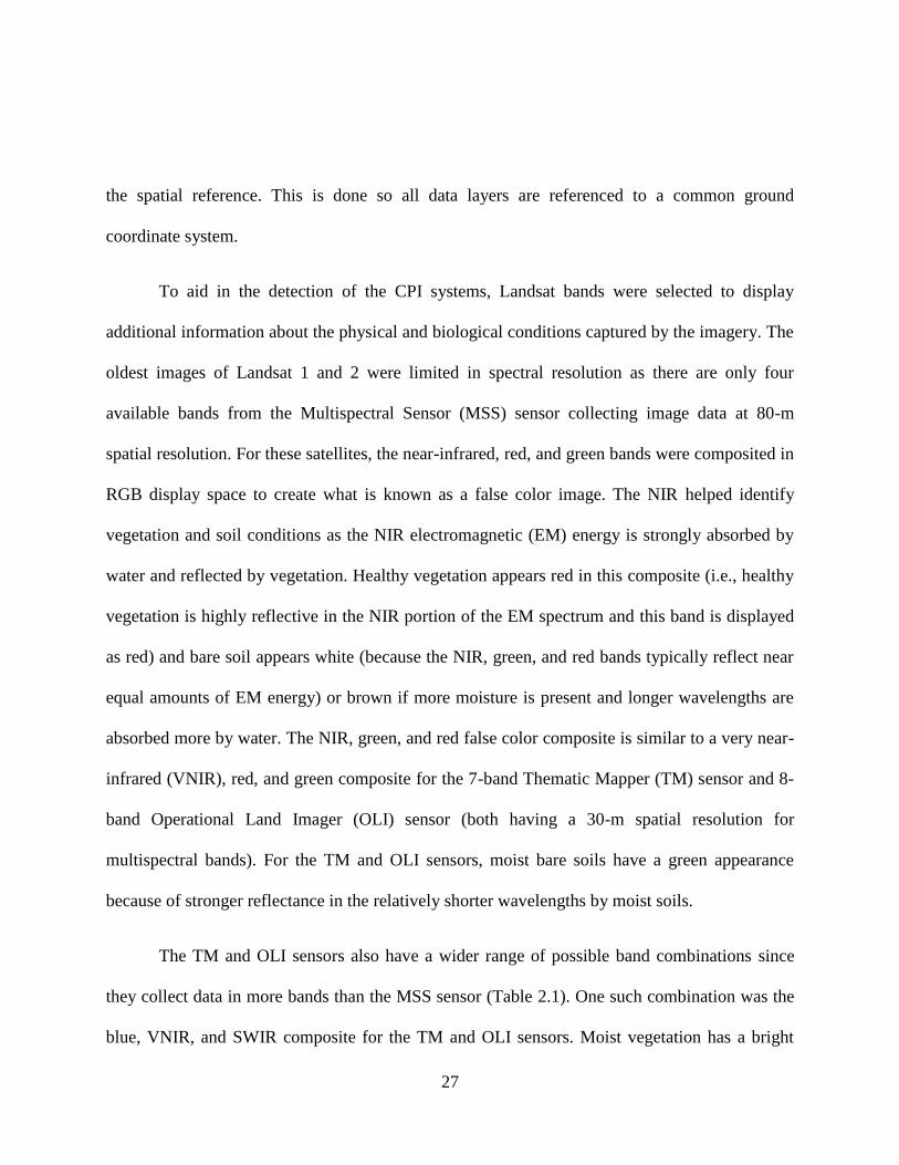
To aid in the detection of the CPI systems, Landsat bands were selected to display
additional information about the physical and biological conditions captured by the imagery. The
oldest images of Landsat 1 and 2 were limited in spectral resolution as there are only four
available bands from the Multispectral Sensor (MSS) sensor collecting image data at 80-m
spatial resolution. For these satellites, the near-infrared, red, and green bands were composited in
RGB display space to create what is known as a false color image. The NIR helped identify
vegetation and soil conditions as the NIR electromagnetic (EM) energy is strongly absorbed by
water and reflected by vegetation. Healthy vegetation appears red in this composite (i.e., healthy
vegetation is highly reflective in the NIR portion of the EM spectrum and this band is displayed
as red) and bare soil appears white (because the NIR, green, and red bands typically reflect near
equal amounts of EM energy) or brown if more moisture is present and longer wavelengths are
absorbed more by water. The NIR, green, and red false color composite is similar to a very near-
infrared (VNIR), red, and green composite for the 7-band Thematic Mapper (TM) sensor and 8-
band Operational Land Imager (OLI) sensor (both having a 30-m spatial resolution for
multispectral bands). For the TM and OLI sensors, moist bare soils have a green appearance
because of stronger reflectance in the relatively shorter wavelengths by moist soils.
The TM and OLI sensors also have a wider range of possible band combinations since
they collect data in more bands than the MSS sensor (Table 2.1). One such combination was the
blue, VNIR, and SWIR composite for the TM and OLI sensors. Moist vegetation has a bright

28
green appearance in this composite and moist soil appears dark purple in this composite. The
purple appearance is due to the equal information (i.e., reflectance) captured by blue and SWIR
bands (thereby displaying as equal levels of red and blue). There was a trial and error process to
determine which combination of bands produced the best visual results for identifying CPIs and
sometimes it was necessary to toggle between displaying several different band combinations in
order to enhance the visual display of vegetation and levels of soil moisture. In addition, multiple
bands of satellite images can be manipulated to calculate several different vegetation indices.
One such index calculated in this study was the Tasseled Cap Transformation (Crist 1985, Huang
et al. 2002). Calculating the tasseled cap indices gave a measure of the brightness, greenness, or
wetness of a pixel in the Landsat image. This process involved a linear combination of the six
bands used in the analysis with coefficients for the transformation given by Huang et al. (2002).
The brightness, greenness, and wetness indices were then composited in different combinations
to display spectrally enhanced images. This process produced the greatest contrast between the
CPI systems and background vegetation, but was also the most labor intensive in terms of
processing time. A RGB composite of the brightness, wetness, and greenness indices resulted in
bare soil appearing red, wet soils appearing blue, and CPI systems with a white appearance due
to about equal reflectance of bright and exposed bare ground, wet soils and healthy vegetation.
Figure 2.2 provides a comparison of Landsat images of Miller County, Georgia illustrating some
of the different display composites used to identify CPIs.
To capture the CPI systems in the composited Landsat scenes, circular irrigated areas
were manually digitized using a procedure known as heads-up digitization. This procedure

29
involves visual (i.e., manual) interpretation of CPIs and using a mouse-controlled cursor to draw
a vector polygon surrounding features in the raster images as displayed on a computer monitor.
This method was used to create a digital boundary of CPI systems identified in the Landsat
imagery. Interpretation and digitization for all images of all years was conducted by the same
analyst. Although this significantly increased the length of manual labor, this was a necessary
step to keep the human bias consistent through all years and allow analysis of changes over time
and the calculation of ground area of the digitized CPI systems. This created a CPI shapefile for
each year analyzed that can be easily disseminated to other end users, or a database of CPI
systems that can be modified and updated as others see fit.
2.4 Results
This section presents data depicting the spatio-temporal evolution of areas equipped for
irrigation in the Coastal Plain as well as the total increase in CPI systems during the 38-year
analysis period of 1976 to 2013. The ability to detect CPI systems at the sub-county level allows
for insight as to which counties have the highest total acreage irrigated and what percentage of
the total land area is irrigated for each county. If a pivot spanned several counties, the digitized
polygon was split and then assigned to the county that it fell in and the area was calculated for
that portion.
There was considerable growth in the areas equipped for irrigation and the number of CPI
systems detected. In 1976, there were 247 CPI systems detected totaling 17,162 hectares (ha)
(Figure 2.3). Those numbers increased to 11,439 CPI systems (Figure 2.3) detected totaling
378,885 ha (Figure 2.3) in 2013. This accounts for an approximate 4,500% increase in CPI

30
systems detected and an approximate 2,000 in total acres irrigated over the 38-year analysis
period. The data suggest that there were smaller pivots being added as the years progressed. The
largest percent changes in CPI systems detected and total acreage were from 1980 to 1984 where
there was a 151% and 145% increase, respectively (Figure 2.4). The percent changes for those
particular years also coincide with a sensor change for the Landsat satellite program (i.e., the 80-
m pixel Multispectral Sensor was replaced by the 30-m Thematic Mapper sensor), which could
introduce increases in detection rates and acres irrigated because smaller CPIs were visible in
these images. An increasing trend of acres irrigated was identified in all years analyzed, although
the rate of increase was not as great as the time period between 1980 and 1984. The percent
change in CPI systems and total acreage was positive for all years analyzed, with the rate of
change drastically slowed after 1984. The time period between 1992 and 1996, produced the
lowest percent change of any other time period. During this time there was an 11% change in
CPI systems detected and an 8% change in total acreage. Initially, there was congruency between
the percent change between the CPI systems and total acreage. After 1988, the difference
between the two metrics increased. The largest difference occurred between 2004 and 2008,
when there was a 58% increase in CPI systems compared to a 27% in total acreage. This
suggests that there was a preference to install smaller CPI systems as previously mentioned.
Initially, southwest Georgia was identified as a region of dense irrigation in the images that
were analyzed. There were a few other sporadic areas of irrigation throughout the analysis
region, but from the onset, southwest Georgia was the core of heavy irrigation in the state. In
particular, the counties of Seminole, Decatur, Miller, Baker, and Mitchell contained the most

31
irrigation. Even as the number of CPI systems and total acreage progressed northeastward, the
southwest Georgia region remained the most densely irrigated. Maps were generated for each
year analyzed, but for brevity the years 1976, 1996, and 2013 are presented (Figures 2.5-2.7).
These three time periods represent the initial date in the time series (1976); a time around the
midpoint of the 38 year analysis period (1996); and the last date of the time period (2013).
Starting with the 1976 time period (Figure 2.5), as previously mentioned southwest Georgia
contained the most CPI systems and total acreage irrigated. The total number of CPIs identified
for the time period was 247, which resulted in 17,567 hectares irrigated. The counties of
Seminole and Decatur were the most densely irrigated at this time. The average sizes of CPI
systems are 71 hectares with the largest CPI systems covering 150 hectares. At the midpoint in
1996 (Figure 2.6), the number of CPI systems detected increased to 3,189. The largest CPI
system covered 231 hectares, with a mean size of 53 hectares. During the 1996 period, densely
irrigated areas expanded north and northeast of Seminole and Decatur counties. The counties of
Miller, Baker, and Mitchell joined Seminole and Decatur as the counties with the highest
irrigation density. The final time period, 2013 (Figure 2.7), had a total of 11,439 CPI systems
that totaled 378,885 hectares. Visually, there is a substantial increase in total acreage in the
eastern part of the Coastal Plain (Atlantic/Lower), but the western part of the Coastal Plain
(Gulf/Upper/Lower) remains the most heavily and densely irrigated. The eastward expansion of
acres irrigated was seen in each subsequent year during the analysis period. From the initial date
analyzed to the last year analyzed, the geographic region that is the most densely irrigated is
southwest Georgia. The region is a part of the Apalachicola Flint Chattahoochee (ACF) River
Basin as irrigation represents the largest use of consumptive water in the Flint River Basin. The

32
largest CPI system found covered 232 hectares and the mean size also decreased to 33 hectares.
The decrease in the mean size of CPI systems corroborates the initial speculation of smaller sized
CPI systems in subsequent years.
To assess the counties that are the most densely irrigated, the percent of total land area and
the total acreage irrigated are analyzed. It is expected that counties with a larger land area have
the capacity to irrigate more. This does not necessarily mean that large counties are the most
densely irrigated. Figures 2.8 and 2.9 highlight the counties with the highest totals in both areas.
These figures also show that southwest Georgia is the most intensely irrigated area of the state.
Southwest Georgia lies within the Flint River Basin, which along with the Central and Coastal
regions of the Coastal Plain of Georgia comprise about 95% of crop production and irrigated
acreage in the state (Guerra et al 2005). During the growing season, irrigation accounts for
approximately 90% of water used in the Flint River Basin. Of the counties that were analyzed in
the Coastal Plain, approximately seventeen had 8,000 hectares or greater irrigated (Figure 2.8) in
the final year of analysis. Using 1984 as a starting point to consider data captured from Landsat
satellite sensors of the same spatial resolution (30-m) between periods of analysis, many of these
counties doubled the total acres irrigated during the 30-year period. Only two of those counties,
Burke County and Jefferson County, are located outside of Southwest Georgia. Eleven of those
seventeen counties currently have, with some counties extending back to 1984, approximately
10% of their total land area equipped for irrigation (irrigated) (Figure 2.9). Seven of those eleven
counties have approximately 15% or more of their total land area equipped for irrigation.
Decatur County (Lower Flint) has the highest number of total acres equipped with 30,127 ha.
33
Seminole County has the highest total percentage of land area irrigated with approximately 35%
of the total land area. Decatur and Seminole Counties along with five other bordering counties
(Baker, Calhoun, Early, Miller, and Mitchell) combined for 146,006 ha. Combined, those seven
counties account for approximately 38% of the 2013 total acreage of CPI.
2.5 Discussion
All studies have some limitations due to data challenges, time constraints, or other
confounding factors. This study shares some of those same challenges, with one of the greatest
limitations being introduced by the data provided by the Landsat satellite program. The changes
in sensors and resolution between Landsat missions could introduce spurious trends. This is not a
challenge that is unique to this particular study. Also there was the nature of how the satellite
images were analyzed visually to manually delineate CPIs. It would have been beneficial to
create an automated detection method, but several attempts to automate the process were not
successful. Manual digitization resulted in labor intensive detection of CPI systems, which was
further compounded by the overall size study area. All digitization of CPI systems in the study
were done by one individual in order to keep consistency from one year of analysis to another.
Visual interpretation studies are often suited for local studies, but were used for regional analysis
in our case. The Landsat satellite program was designed to detect changes in land cover and land
use, but the sensors used and resolution available changed through time. These changes could
introduce spurious increases in CPI systems detected, but this issue was not unique to our study
and is common in all studies that span the same time period as our analysis. There were other

34
remotely sensed products available, such as aerial photography, but it was determined that
Landsat was the optimal mix of temporal and spatial coverage for our analysis.
Alternative forms of aerial photographs include the National High Altitude Photography
(NHAP) program, the National Aerial Photography Program (NAPP), and the National
Agriculture Imagery Program (NAIP) produced by the United States Department of Agriculture..
NAIP imagery has been used for prior agricultural studies in the region. NAIP acquires areal
imagery during the agricultural growing seasons in the continental USA. The first images were
collected in 2003 and are available in 5-year intervals if funding is available (USDA 2015). The
difference is spatial coverage between NAIP imagery and Landsat can be seen in Figure 10. Each
Landsat scene is approximately 185 km x 185 km compared to the approximate 10 km by 10 km
size of the NAIP imagery. NAIP imagery yields more detail, but the advantage of using Landsat
images is the ability to cover a larger area for a much longer period of time. There would also be
a large increase in the pre-processing necessary to create spatial references for numerous older
aerial photographs. Landsat also has a higher temporal resolution compared to other forms of
aerial photographs available. The ability to detect CPI systems smaller than 12 acres (5 hectares)
was a limiting factor of the spatial resolution of the Landsat sensor. There were also attempts to
automate the detection process through Houghton transformation and other circle detection
techniques, but none produces adequate results.
Overall there was a positive trend in the number of CPI systems detected and the total
acreage. Our analysis indicated that within the overall positive trend, there were year to year
decreases in the rate of change. The slowdown in the rate of change could be tied to various

35
policies implemented in the state. One of the first policy changes was the introduction of the
agricultural sector of the state was the Conservation Reserve Program (CRP) beginning in the
1980s. This program was part of the 1985 Farm Bill and was in effect from 1985 - 1992. The
objective of the CRP program was to convert marginal cropland to a less intensive use, primarily
trees, as 645,931 acres have been planted since 1986 (Center for Invasive Species and Ecosystem
Health, the University of Georgia, 2005). This program was incentivized, paying farmers an
average of $42.30 per acre (Center for Invasive Species and Ecosystem Health, the University of
Georgia, 2005). Most of the land converted in the CRP program in Georgia was released in 1996,
meaning that the landowner was free to use the land as they saw fit. The implementation of this
policy also coincided with a drastic slowdown in the acres irrigated. As previously mentioned,
from 1984 to 1996 there was a decrease in the percent change of CPI systems and total acreage.
Farmers may have seen this land conversion as a more profitable long-term solution over
marginal agricultural land cover.
Coinciding with the timing of the CPR program were amendments in 1988 to Georgia’s
Groundwater Use Act of 1972 and Water Quality Control Act that required a permit to be
obtained for agricultural water users who used more than 100,000 gallons per day on a monthly
basis. The permits were provided and recorded by the Georgia Environmental Protection
Division (EPD). The highest irrigation rates typically occur within the Flint and Chattahoochee
River Basins. This area is part of an ongoing dispute between the states of Alabama, Florida, and
Georgia known as the tri-state water wars. The tri-state water wars are between based on water
rights in the Alabama-Coosa-Tallapoosa (ACT) and Apalachicola-Chattahoochee-Flint (ACF)

36
River Basins. Although this dispute was not initially tied to agricultural water use, some of the
litigation spurred policy changes that may have acted to curtail the initial rapid increase that was
seen in irrigated acreage in Georgia. It is also important to note that the Flint River Basin has
some of the highest agricultural water withdrawals in Georgia. Much of the water is from the
Floridian aquifer (Spurgeon and Mullen, 2005).
A few changes included legislation that required CPI systems to be 80% efficient by
January 1st 2020 and the Georgia EPD’s intentions to produce a 20% reduction in agricultural
water withdrawals in the Flint River Basin and the state’s ability to restrict agricultural water
withdrawals during periods of drought (Masters et al. 2009). As there are still ongoing efforts to
accurately monitor the amount of water used in the agricultural sector throughout the state, this
also created a desire for Georgia to quantify the amount of water used in the agricultural sector
and create guidelines for farmers on how much water to withdraw to during periods of drought.
To answer those questions, it is vital to know how irrigation varies spatially and how irrigation
has varied over time. This work provides some critical information to answer both of those
questions as our results present acres irrigated in a historical context and provides that
information spatially over a 38-year time period, as opposed to a tabular format.
2.6 Conclusion
This analysis conducted a simple visual interpretation technique of Landsat satellite images
to assess the spatio-temporal evolution of areas irrigated in the Georgia Coastal Plain. Acres
irrigated were estimated through identifying center-pivot irrigation systems throughout the
analysis region. Other research has suggested that this region has experienced upward increases

37
in areas irrigated, but there are few studies that display the long term spatial extent of this
increase. As expected, there were significant increases in the total acres irrigated and the number
of CPI systems detected in the Georgia Coastal Plain over our 38-year analysis period. There was
an approximate 4,500% increase in CPI systems detected and an approximate 2,000% increase in
total acres irrigated during the length of our analysis. The largest increases took place between
1980 and 1984 and there were steady year to year increases as well, although there was a
dramatic slowdown in the rate of increase from 1984 to 1996. This slowdown in the rate of
increase was primarily due to legislation introduced around the late 1980s such as incentive
laden legislation to convert marginal agricultural land cover to a forested land cover and
legislation that required permits for agricultural water withdrawals and placed restrictions on
withdrawals during periods of drought. The results showed that southwest Georgia is the most
densely irrigated portion of the state as there were seven counties in this area that accounted for
38% of the 2013 total acres irrigated. Ease of access to sustainable water sources, suitable soils
that promote crop growth, and level topography are a few potential reasons for irrigation
favoring southwest Georgia. Two counties in particular, Decatur and Seminole Counties, have
the most total acres irrigated and highest percentage of total land irrigated respectively. These
counties lie within the ACF River Basin, with is currently at the center of legal dispute over
water rights between Alabama, Florida, and Georgia. This research will serve as a tool to aid
others in the scientific community identify any ecological, climatic, or water resource impacts
this increase in irrigation may have presented, as this work will serve as a baseline for spatio-
temporal changes in irrigation in the Georgia Coastal Plain.

38
2.7 References
Adegoke, J., Pielke, R., Eastman, J., Mahmood, R., & Hubbard, K., 2003. Impact of Irrigation on
Midsummer Surface Fluxes and Temperature under Dry Synoptic Conditions: A
Regional Atmospheric Model Study of the U.S. High Plains. Monthly Weather Review,
131, 556-564.
Barnes, F., & Keyes, A., 2010. Georgia's Water Conservation Implementation Plan. GA:
Georgia Department of Natural Resources Environmental Protection Division, pp. 1-
204.
Barnston, A., & Schickedanz, P., 1984. The Effect of Irrigation on Warm Season Precipitation in
the Southern Great Plains. J. Climate Appl. Meteor. Journal of Climate and Applied
Meteorology, 23, 865-888.
Boken, V., Hoogenboom, G., Hook, J. E., Thomas, D. L., & Guerra, L. C., 2004. Agricultural
water use estimation using geospatial modeling and a geographic information system.
Agricultural Water Management, 67(3), 185-199.
Boucher, O., Myhre, G., & Myhre, A., 2004. Direct human influence of irrigation on
atmospheric water vapour and climate. Climate Dynamics, 22, 597-604.
Braneon, C., Georgakakos, Peter, A., 2011. Climate Change Impacts on Georgia Agriculture and
Irrigation. Proceedings of the 2011 Georgia Water Resources Conference, 11-13 April
2011, Athens, Georgia (Georgia Institute of Technology, Warnell School of Forestry and
Natural Resources, The University of Georgia), pp. 1-2.
Braneon, C., 2014. Agricultural Water Demand Assessment in the Southeast U.S. Under Climate

39
Change, Ph.D. dissertation, Georgia Institute of Technology, 240 p.
Center for Invasive Species and Ecosystem Health, the University of Georgia., 2005. Land Use
When CRP Payments End - What History Tells Us in Georgia. Retrieved November 20,
2015, from http://www.bugwood.org/crp/landuse.html
Cook, B., Shukla, S., Puma, M., & Nazarenko, L., 2014. Irrigation as an historical climate
forcing. Clim Dyn, 44, 1715-1730.
Deangelis, A., Dominguez, F., Fan, Y., Robock, A., Kustu, M., & Robinson, D., 2010. Evidence
of enhanced precipitation due to irrigation over the Great Plains of the United States.
Journal of Geophysical Research, 15, D15115.
ESRI., 2007. ArcGIS Desktop Help 9.2 - welcome. URL:
http://webhelp.esri.com/arcgisdesktop/9.2/index.cfm?TopicName=welcome, ESRI,
Redlands, CA (last date accessed: 6 July 2015)
Evans, J., & Cohen, M., 2009. Regional water resource implications of bioethanol production in
the Southeastern United States. Global Change Biology, 15(9), 2261-2273.
Evenson, R., & Gollin, D., 2003. Assessing the Impact of the Green Revolution, 1960 to 2000.
Science, 300, 758-762.
Geerts, B., 2002. On the effects of irrigation and urbanisation on the annual range of monthly-
mean temperatures. Theoretical and Applied Climatology, 72(3/4), 157-163.
Guerra, L., Garcia, A., Hook, J., Harrison, K., & Boken, V., 2005. Impact of local weather
variability on irrigation water use in Georgia. Proceedings of the 2005 Georgia Water
Resources Conference, 25-27 April 2005, Athens, GA (University of Georgia,

40
University of Mississippi, Geoinformatics Center), pp. 1-4.
Hodler, T., & Schretter, H., 1986. The atlas of Georgia. Institute of Community and Area
Development, University of Georgia. Athens, GA, 273 p.
Hook, J., 2010. Georgia WPR - Ag Water Demand - SW & GW Demand by WPR, URL:
http://www.nespal.org/SIRP/waterinfo/State/AWD/AgWaterDemand_By_WPR.html
(last date accessed: 1 November 2015)
Huang, C., Wylie, B., Yang, L., Homer, C., & Zylstra, G., 2002. Derivation of a tasseled cap
transformation based on Landsat 7 at-satellite reflectance. International Journal of
Remote Sensing, 36(2), 1741-1748.
Jensen, J. R., 2005. Introductory digital image processing: A remote sensing perspective (3rd
ed.). Pearson Prentice Hall, Upper Saddle River, NJ, 343 p.
Kottek, M., Grieser, J., Beck, C., Rudolf, B., & Rubel, F., 2006. World Map Of The Köppen-
Geiger Climate Classification Updated. Meteorologische Zeitschrift, 15(3), 259-263.
Kueppers, L., Snyder, M., & Sloan, L., 2007. Irrigation cooling effect: Regional climate forcing
by land-use change. Geophysical Research Letters Geophys. Res. Lett., 34(3), L03703.
Lobell, D., & Bonfils, C., 2008. The Effect of Irrigation on Regional Temperatures: A Spatial
and Temporal Analysis of Trends in California, 1934–2002. Journal of Climate J.
Climate, 21(10), 2063-2071.
Masters, M., Cummings, R., Daniels, B., Rowles, K., & Wilson, D., 2009. Managing
Agricultural Water Use During Drought: An Analysis of Contemporary Policies
Governing Georgia’s Flint River Basin. Sea Grant Law and Policy, 2(1).

41
Minchenkov, A., 2009. USDA study finds 54.9 million acres of U.S. Farmland now irrigated,
USDA News Release, URL:
http://www.usda.gov/wps/portal/usda/usdahome?contentid=2009/12/0596.xml, United
States Department of Agriculture, Washington, DC (last date accessed: 1 November
2015)
Ozdogan, M., & Gutman, G., 2008. A new methodology to map irrigated areas using multi-
temporal MODIS and ancillary data: An application example in the continental US.
Remote Sensing of Environment, 112(9), 3520-3537.
Ozdogan, M., Yang, Y., Allez, G., & Cervantes, C., 2010. Remote Sensing Of Irrigated
Agriculture: Opportunities And Challenges. Remote Sensing, 2(9), 2274-2304.
Pervez, M., & Brown, J., 2010. Mapping Irrigated Lands at 250-m Scale by Merging MODIS
Data and National Agricultural Statistics. Remote Sensing, 2(10), 2388-2412.
Ramankutty, N., Evan, A., Monfreda, C., & Foley, J., 2008. Farming the planet: 1. Geographic
distribution of global agricultural lands in the year 2000. Global Biogeochem. Cycles
Global Biogeochemical Cycles, 22(1), GB1003.
Roy, S., Mahmood, R., Quintanar, A., & Gonzalez, A., 2010. Impacts of irrigation on dry season
precipitation in India. Theoretical and Applied Climatology, 104(1/2), 193-207.
Rundquist, D., Hoffman, R., Carlson, M., & Cook, A., 1989. The Nebraska center-pivot
inventory - An example of operational satellite remote sensing on a long term basis.
Photogrammetric Engineering & Remote Sensing, 55, 587-590.
Shukla, S., Puma, M., & Cook, B., 2013. The response of the South Asian Summer Monsoon

42
circulation to intensified irrigation in global climate model simulations. Clim Dyn
Climate Dynamics, 21-36.
Southeastern Regional Climate Center (SERCC)., 2015. Monthly and Seasonal Climate, URL:
https://www.sercc.com/climateinfo/monthly_seasonal (last date accessed: 7 July 2015)
Spurgeon, K., & Mullen, J., 2005. Estimating the Value of Irrigation Water in Georgia.
Proceedings of the 2005 Georgia Water Resources Conference, 25-27 April 2005,
Athens, GA (Georgia Institute of Technology, Institute of Ecology, The University of
Georgia), pp. 1-3.
Tilman, D., 1999. Global environmental impacts of agricultural expansion: The need for
sustainable and efficient practices. Proceedings of the National Academy of Sciences,
96(11), 5995-6000.
Tilman, D., 2001. Forecasting Agriculturally Driven Global Environmental Change. Science,
292(5515), 281-284.
UN Department of Economic and Social Affairs., 2015. World population projected to reach 9.7
billion by 2050, URL: https://www.un.org/development/desa/en/news/population/2015-
report.html, United Nations, New York (last accessed: 11 January 2016)
USDA., 2015. National Agricultural Imagery Program (NAIP) Imagery. URL:
http://www.fsa.usda.gov/programs-and-services/aerial-photography/imagery-
programs/naip-imagery/, United States Department of Agriculture Farm Service Agency,
Washington, DC (last date accessed 12 November 2015)
USGS. (2015). Landsat Missions: Imaging the Earth Since 1972, URL:

43
http://landsat.usgs.gov/about_mission_history.php, U. S. Geological Survey (last date
accessed: 6 July 2015)
Ustin, S. L., & American society for Photogrammetry and remote Sensing., 2004. Remote
sensing for natural resource management and environmental monitoring (3rd ed., Vol.
4). Lewis Publishers, Hoboken New Jersey, 736 p.
Velpuri, N., Thenkabail, P., Gumma, M., Biradar, C., Dheeravath, V., Noojipady, P., & Yuanjie,
L., 2009. Influence of Resolution in Irrigated Area Mapping and Area Estimation.
Photogrammetric Engineering & Remote Sensing, 75(12), 1383-1395.
Williams, M. D., Goodrick, S. L., Grundstein, A., & Shepherd, M., 2015. Comparison of dew
point temperature estimation methods in Southwestern Georgia. Physical Geography,
36(4), 255-267.

44
Table 2-1: Table providing information on the Landsat missions used in analysis

45
Figure 2.1: Physiographic provinces of Georgia

46
Figure 2.2: Natural, False, and Brightness, Wetness and Greenness (BWG) tasseled cap composites of Miller Country,
Georgia, USA
Figure 2.3: Total center pivot systems and acreage irrigated (hectares)

47
Figure 2.4: Percent change in center pivot irrigation systems (blue) and total acreage (red).

48
Figure 2.5: Map of 1976 CPI systems overlaid on a Landsat false color composite. The variations in the hue are due to the
composite pulling from scenes from different dates.

49
Figure 2.6: Map of 1996 CPI systems overlaid on a Landsat composite of tasseled cap indices.

50
Figure 2.7: Map of 2013 CPI systems overlaid on Landsat false color composite.

51
Figure 2.8 County breakdown of total hectares irrigated for 2013

52
Figure 2.9 County breakdown of percent of total land area irrigated for 2013

53
Figure 2.10 Map of NAIP imagery compared to a Landsat scene.

54
3) COMPARISON OF DEW POINT TEMPERATURE ESTIMATION METHODS
IN SOUTHWESTERN GEORGIA
Williams et al., 2015: Comparison of Dew Point Temperature Estimation Methods in
Southwestern Georgia. Physical Geography, in press, DOI:10.1080/02723646.2015.1011554

55
Abstract
Recent upward trends in acres irrigated in the United States have been linked to increasing
low level surface moisture. Unfortunately, stations with dew point data for monitoring low-level
moisture are sparse. Thus, models that estimate dew points from more readily observed data
sources are useful. Daily average dew temperatures were estimated and evaluated at 14 stations
in southwest Georgia using linear regression models and artificial neural networks. Estimation
methods were drawn from simple and readily available meteorological observations, therefore
only temperature and precipitation were considered as input variables. The 14 weather stations
were equally partitioned into seven training stations and seven independent stations. In total three
linear regression models and 27 artificial neural networks (ANN) were analyzed for the 14 sites.
The two methods were evaluated using root mean square error, mean absolute error, the
Pearson’s correlation coefficient, the Index of Agreement, and the Coefficient of Efficiency to
assess the skill of the estimation methods. Both methods produced adequate estimates of daily
averaged dew point temperatures, with the artificial neural network displaying the best overall
skill. Both methods displayed optimal performance for warmer dew point temperatures and
showed poorer skill estimating lower dew point temperatures. The depredated skill for low dew
point values is likely due to the small sample of observations around the lower dew point ranges.
On average the ANN reduced root mean square error by 6.86% and mean absolute error by
8.30% when compared to the best performing linear regression model.

56
3.1 Introduction and Literature Review
Changing land cover can have important effects on local climate (Pielke et al. 2002,
Shepherd et al. 2002, Marshall et al. 2004, Mahmood et al. 2013). The state of the land cover
directly influences how incoming solar radiation is partitioned into other energy budget terms,
such as sensible and latent heat. Agriculture is a predominate form of land cover, accounting for
nearly 18 million km2 (Ramankutty et al. 2006), or roughly 40% of the global land cover (Foley,
2005). Agricultural land cover is expected to increase with projected rises in population and the
growing demand for biofuel production (Evans and Cohen 2009). While some agricultural
landscapes rely on natural precipitation for irrigation, there has been rapid growth towards
artificially irrigated landscapes (Harrison 2001, Tillman 2001). This introduction of water at the
surface has the ability to change the low level near surface moisture content (Ferguson and
Maxwell 2011). Increased low level moisture has been linked to the 1995 and 1999 Midwestern
heat waves (Changnon et al 2003). Hot humid weather can cause heat stress in humans (Gaffen
and Ross 1998), increasing their chances of experiencing heat related morbidity or mortality
(Bently and Stallins 2003, Lipmann et al., 2013). It is difficult to assess these postulated changes
in moisture content because of the lack of sufficient data outside of first order observation
stations. Thus, there is a need to model and estimate low level moisture from readily available
meteorological data.
Early methods for estimating low level moisture involved using daily minimum
temperature as a proxy for dew point temperature. This assumption is not always valid if there
are large diurnal variations in dew point temperature and if minimum temperature stays well
57
above dew point temperature (Kimball et al. 1997). Kimball et al. (1997) used annual
precipitation, potential evapotranspiration, mean daily net solar radiation, as well as temperature
(maximum, minimum, and mean) to produce a more accurate assessment of daily dew point
temperature across the United States and Alaska, primarily at first order observation stations.
Hubbard et al. (2003) expanded on the efforts of Kimball and evaluated an additional four
regression equations for the Northern Great Plains in the United States. The goal of their study
was to produce a dew point temperature estimation method that required less complex input data
than Kimball et al. (1997). They wanted to take advantage of meteorological data provided by
the National Weather Service Cooperative (NWS Coop) weather stations. Their analysis found
that a combination of maximum (Tx), minimum (Tn), and mean (Tm) temperature are the best
estimators for daily dew point temperature. An alternative method for estimating low level
moisture is through artificial neural networks (ANN). Jain et al. (2008) estimated
evapotranspiration (ET) using an ANN from limited input variables. Their estimation model
included hourly temperature, dew point, sunshine radiation, wind speed, and humidity in
Reynolds Creek Experimental Watershed. Shank et al. (2008) developed ANN models to predict
dew point temperature at two hour intervals, up to 12 hours in advance. Their methods
incorporated dew point temperature, relative humidity, vapor pressure, wind speed, and solar
radiation from the Georgia Environmental Automated Monitoring Network (GEAMN) to
develop and train the ANN.
The purpose of this study is to estimate daily dew point temperature using linear regression
models and an ANN for portions of Southwest Georgia using daily meteorological data, an

58
understudied area that has undergone rapid agricultural expansion since the 1970s (Harrison
2001). This study aims to give insight into which meteorological variables sufficiently estimate
dew point temperature in the analysis region. A secondary objective is to evaluate the
performance of the linear regression models in an area outside of the Great Plains to determine if
there are any differences in the variables needed to successfully estimate dew point temperature.
Southwest Georgia experiences a higher amount of annual precipitation than the Great Plains and
also suffers from less continentality (Rohli and Vega 2008). Precipitation could be an important
factor in estimating daily dew point, as the highest dew point ever recorded in the United States
was partly caused by heavy rains the morning of the event (NWS WFO Grand Forks, ND).
Shank et al (year?) gave insight as to how an ANN performed in the region from an error
standpoint, but their analysis included observed dew point temperatures as an input variable.
This study analyzes a different geographic location from Hubbard et al. (2003) and focuses on a
smaller spatial extent than Kimball et al. (1997). The ANN analysis is not aided by the inclusion
of dew point temperature or any moisture parameter because the focus is on producing a daily
estimate versus a prediction. Qualitative comparisons of the performance of the two estimation
techniques are assessed from an error standpoint. The development of a valid estimation
technique is a vital step in the goal of characterizing the influence of irrigation on climate in the
study region. This region has experienced rapid growth in acres irrigated (Harrison 2001), but
little is known about the influence of irrigation on the climate. This research will provide a tool
to answer the question about the impact of irrigation in the region. Section 3.2 will provide a
description of the data and methodology applied which entails a breakdown of the linear

59
regression and ANN models. This is followed by the results and discussion section, where the
performance of each method is evaluated, and then the conclusion.
3.2 Data and Methodology
Data
The dataset used in this study is the Georgia Automated Environmental Monitoring
Network (GEAMN, Hoogenboom 2000). The GAEMN, established in 1991, is maintained by
the University of Georgia and has a 1s temporal resolution that is aggregated into 15 minute
averages or totals. There are over 75 stations in the network throughout Georgia that record
weather variables including air temperature, relative humidity, vapor pressure, wind speed and
direction, and solar radiation. Dew point temperature is calculated from the collected variables.
This study uses daily aggregates of maximum and minimum temperature, precipitation, and dew
point.
Linear Regression
The regression equations are adapted from Hubbard et al. 2003, hereafter referred to as
H03. H03 was developed using station data in the Great Plains region. The analysis herein
employed three out of the five total regression equations developed by H03. The equations used
are as follows:
H03 Method 1: T_d= ∝(T_n )+ β(T_x-T_n )+ γ (1)
H03 Method 3: T_d= ∝(T_m )+ β(T_n )+ γ(T_x-T_n )+ λ (2)

60
H03 Method 4: 〖 T〗_d= ∝(T_n )+ β(T_x-T_n )+ γ(P_daily )+ λ (3)
Where Dew point temperature, Tx, Tn, Tm, and Pdaily are the daily dew point temperature;
maximum, minimum, and mean daily temperature; and daily precipitation, respectively. The
coefficients of the regression equations are represented by ∝,β,and, β, and λ. Figure 3.1 shows
the GEAMN stations used in this study. The stations labeled in blue represent the stations used in
the development of the regression models and the stations labeled in red represent the
independent stations. Method 1 (eqn. 1) uses minimum temperature and the diurnal temperature
range (DTR) to estimate dew point. Method 3 (eqn. 2) includes the mean temperature in addition
to the minimum temperature and the DTR. Method 4 (eqn. 3) uses minimum temperature, DTR,
and daily precipitation to estimate daily dew point temperature.
Different configurations of precipitation were also included in equation 3, in place of the
P_daily variable, to determine if there was any improvement in model skill. The different
configurations include three, five, and seven day totals and averages. The different
configurations of precipitation showed no improved model skill, so P_daily is the primary
configuration of precipitation used in the analysis.
To determine the coefficients for the regression models and to evaluate the initial
performance of the regression models, a subset of seven stations with the longest continuous
period of record within the region (Figure 2.1, blue) is selected. The data from the seven stations
are aggregated to determine the coefficients only, and then each station is analyzed on an
individual basis. The performances of the three models are evaluated for each station before

61
choosing the best model to perform test on independent data not used in model training. The
independent stations in the analysis (figure 2.1, red) are not used in the development of the
model coefficients or in the initial estimates of the model performance. The model evaluation
parameters presented in this analysis are selected to ensure a robust viewpoint of possible error
and biases, and to avoid solely relying on correlation parameters as high correlations can be
achieved by poor models (Legates and McCabe, 1999). The three models are evaluated using the
root mean square error (RMSE), the mean absolute error (MAE), the Pearson’s correlation
coefficient (R), the Index of Agreement (d), and the Coefficient of Efficiency (E). Readers are
encouraged to review Legates and McCabe (1999) for a detailed overview of the d and E model
validation statistics. As previously stated, a single set of coefficients is developed from a
combination of the seven developmental stations. The decision to merge the data sets is made to
ensure the models can adequately estimate dew point temperatures for varying climatic regimes
within the region.
Artificial Neural Network
The ANN used in this study is a feed-forward multilayer perceptron (algorithm) with one
hidden layer using sigmoid activation functions and trained using back-propagation as
implemented in pyBrain version 0.3.1 (Schaul et al. 2010) with python programming language
version 2.7.3. The basic network design is shown in Figure 2. A number of potential networks
were evaluated. These networks differ in the number of input variables and the number of
processing nodes in the hidden layer. Inputs to the network include minimum temperature,
temperature range, and 0 to 5 days of antecedent precipitation. A constant bias input node with a

62
value of unity is also included. The number of nodes in the hidden layer varies from a minimum
of two to a maximum equal to the number of inputs for the network (up to eight). In total, 27
ANNs are evaluated. Data for ANN training and testing are partitioned in an identical manner to
the regression models.
3.3 Results and Discussion
Linear Regression
The three methods performed comparably from an error and model evaluation standpoint.
The RMSE, MAE, R, d, and E values were only separated by hundredths for all three models for
all stations within the training data set. The Pearson’s correlation coefficient (R), d, and E all
indicate improved performance when they are closer to unity. Overall, Method 4 had the lowest
errors and the highest model evaluation statistics. This was a different result from H03, as
Equation 2 in our analysis was their best performing method. As expected, their analysis region
has a different climatic regime from our analysis region. This result shows that daily
precipitation is an important factor in estimating daily dew point values. As a refresher Equation
3 incorporated minimum temperature, the difference between maximum and minimum
temperature and the addition of daily precipitation. The equation with included coefficients is as
follows:
T_d= 1.00681512(T_n )+ 0.17912155(T_x-T_n )+ 0.05591049(P_daily )- 1.789463 (4)
The results of the model evaluation and error statistics are displayed in tables one through three.
For most of the stations in the developmental dataset, the R, and d statistics were nearly identical

63
amongst the three methods. For most stations R ranged from 0.94 to 0.96. The only noticeable
variation was in the RMSE, MAE, and the E statistic. This speaks to the robustness of the
equations developed by H03. From a physical standpoint, Method 4 accounts for the relationship
between dew point and minimum temperature (Hubbard et al., 2003), the diurnal temperature
range is indicative of the moisture content of an air mass (H03). The inclusion of precipitation
captures the partitioning of energy to latent heating, especially in the summer months when the
atmospheric demand for water is highest.
We observed some biases in the models at high and low dew points. This result was
present in all three methods, although only Equation 3 is shown here. This is captured in the
scatter plot of estimated and observed dew point values from the Arlington automated weather
station (Figure 2.3). Figure 2.3 shows a greater tendency for the model to underestimate values
on the low end of dew point spectrum. Arlington is used as a representative station because it has
the lowest RMSE and MAE for the selected method. Other stations are expected to perform
comparably to the Arlington station. There is also a tendency for the overestimation of dew point
at the high end. Even with the discrepancies mentioned above, Equation 3 does an adequate job
of capturing the observed variability. The overall performance of the model is adequate as well,
as approximately 85% of the estimated values are within 3°C of the observed values (fig. 2.4).
Since the method that included precipitation performed the best, it was a natural inquiry
to see if different variations of precipitation improved the skill of the model. The underlying
premise of this hypothesis is to analyze whether there is a “soil moisture memory” component to
the estimation of dew point, as modeling studies suggest that wet soils are thought to influence

64
ET rates, thus influencing the dew point temperature (Dirmeyer et al. 2009, Dirmeyer et al.,
2012, Koster and Suarez, 2000). To test this theory, three, five, and seven day totals and averages
were added in place of the daily precipitation. It was also required to develop a new set of
coefficients for each variation of precipitation tested. It is possible that the additional days of
precipitation were a poor fit for the regression equations as additional precipitation information
slightly degraded the model performance when compared to the regression model with daily
precipitation (table 2.5).
The model performance was evaluated on an annual basis. This measure was taken to
ensure a robust model performance, capable of handling a wide array of climatic conditions.
Essentially, the model will be applied when irrigation rates are at their highest, the growing
season (April – September). During the growing season, the model displays an improved skill
and has an optimal performance during this period. This was tested by developing a set of
coefficients for October to November for all years. The coefficients of the growing season data
set are then applied to the Arlington training station. The growing season regression model
reduced the RMSE and the MAE by 17% (table 2.5).
Artificial Neural Network
The first step in applying an ANN to the problem of estimating dew point temperature is
to determine the combination of inputs and hidden nodes that provide the best performance. The
number of inputs is dependent upon the number of day’s worth of precipitation data we wish to
include in the analysis and ranges from zero to five. Other inputs included in all networks are

65
minimum temperature, temperature range and a constant bias neuron whose value is always
equal to unity. There is no formula for determining the optimal number of nodes in the hidden
layer of a network. It is generally suggested that the number of hidden nodes should be between
the number of inputs and the number of outputs (Heaton 2013). For this study we will test
networks with number of hidden nodes ranging from 2 to the number of inputs.
Figure 2.5 shows how number of inputs and hidden nodes affected network performance
as expressed by mean absolute and root mean square errors for 27 different networks. Examining
the figure from left to right, the first network (3_2) relies on only minimum temperature and
temperature range to determine dew point. Addition of an additional hidden node (3_3) allows
the network to better fit the data. Addition of the current days precipitation (4_2) allows for
further improvement in the network performance. Expanding the network beyond 4 inputs and 2
hidden nodes did not lead to an appreciable improvement in network performance. For the
remainder of the study the ANN architecture used is that of four inputs (minimum temperature,
temperature range, daily precipitation and a constant) with two hidden nodes.
Overall the ANN outperformed the regression methods of H03 as shown in table 2.6 for the
training data and table 2.7 for the validation data. For all stations the ANN displayed lower error
values and was equal to or better on the other performance metrics as well. Direct comparison
between the ANN and H03 equation 3 shows that on average the ANN reduced RMSE by 6.86%
and MAE by 8.30% (table 2.8). One area where the ANN offered little improvement is for low
dew point temperatures (Figure 6). For dew points in the 20°- 30° C range, the ANN has an
absolute error within 2° C of the observed for 90% of the cases and 60% of the time the error is

66
1° C. However, performance for the lower end of the dew point spectrum drops off quickly.
When the dew points are between 0°-10° C, only 50% of cases are within 2° of the observed dew
point and only 24% within 1° C. Fortunately, the growing season of southwest Georgia is
characterized by dew point values in the range where the ANN estimates are most accurate. Note
that the ANN was not retrained using only growing season data as was done for the regression
model
3.4 Conclusion
The overarching goal of this study was to develop a daily dew point estimation method
adapted for southwest Georgia. An estimation method is needed because of the poor availability
of long term dew point observations in the region. It was also desired to make the estimation
draw from readily available temperature and precipitation observation from NWS COOP stations
in the region. The linear regression equations developed by H03 were adapted and applied to our
region of interest. Three of the five methods used in H03 were used here, with H03 Equation 3
performing the best from an error standpoint. It is reasonable to believe that Equation 3 can be
generalized across the southeast. On average, H03 Equation 3 performed equal to, or better in all
five measures of performance for the training stations (tables 2.1-2.3). It was shown that the
model performs best during the growing season, when irrigation rates are at their highest, and
that additional precipitation information actually degrades model performance. An artificial
neural network (ANN) is also employed to estimate dew point.
Seven automated weather stations from the GEAMN were selected to train and validate
each the estimation model for each technique. On an annual basis the ANN performed best, only

67
bettered by the growing season version of the regression model. A growing season only version
of the ANN was not tested, and is something that can be explored in the future to see if there is
any improvement in the skill of its estimation. Each technique tested performed adequately for
the region and should be able to assist in a retroactive analysis in dew point estimation in the
study region. Estimating dew point from limited meteorological variables has been successfully
demonstrated in the Great Plains region, and now in southwest Georgia. This gives confidence
into the validity of dew point estimates derived from other variables, which can be applied to
construct dew point climatology for data poor regions. The next chapter of this dissertation
applies the estimation method developed here to study the influence of agricultural irrigation in
the region by evaluating changes in dew point. This analysis also presents the ability to
investigate and assess historical trends in dew point temperatures outside of first order station,
which would be the first analyses to date.
3.5 References
Adegoke, J. O., Pielke, R. A., Eastman, J., Mahmood, R., & Hubbard, K. G. (2003). Impact of
Irrigation on Midsummer Surface Fluxes and Temperature under Dry Synoptic
Conditions: A Regional Atmospheric Model Study of the U.S. High Plains. Monthly
Weather Review, 131(3), 556-564.
Harrison, K. A. (Director) (2001, March 26). Agricultural Trends in Irrigation. Proceedings of
the 2001 Georgia Water Resources Conference. Lecture conducted from Institute of
Ecology, Athens.
Bentley, M. L., & Stallins, J. A. (2008). Synoptic evolution of Midwestern US extreme dew
68
point events. International Journal of Climatology, 28(9), 1213-1225.
Changnon, D., Sandstrom, M., & Schaffer, C. (2003). Relating changes in agricultural practices
to increasing dew points in extreme Chicago heat waves. Climate Research, 24, 243-
254.
Deangelis, A., Dominguez, F., Fan, Y., Robock, A., Kustu, M. D., & Robinson, D. (2010).
Evidence of enhanced precipitation due to irrigation over the Great Plains of the United
States. Journal of Geophysical Research, 115(D15), 1-14.
Dirmeyer, P. A., Schlosser, C. A., & Brubaker, K. L. (2009). Precipitation, Recycling, and Land
Memory: An Integrated Analysis. Journal of Hydrometeorology, 10(1), 278-288.
Dirmeyer, P. A., Jin, E. K., Kinter, J. L., Cash, B. A., Manganello, J., Huang, B., et al. (2012).
Evidence for Enhanced Land–Atmosphere Feedback in a Warming Climate. Journal
of Hydrometeorology, 13(3), 981-995.
Evans, J. M., & Cohen, M. J. (2009). Regional water resource implications of bioethanol
production in the Southeastern United States. Global Change Biology, 15(9), 2261-2273.
Foley, J. A. (2005). Global Consequences Of Land Use. Science, 309(5734), 570-574.
Gaffen, D. J., & Ross, R. J. (1998). Increased summertime heat stress in the US. Nature, 396,
529-530.
Heaton, J. (2013). Introduction to Neural Networks for Java (2 ed.). Chesterfield, MO: Heaton
Research Inc.
Hoogenboom, G. (2000). The Georgia automated environmental monitoring network. Preprints
of The 24th Conference on Agricultural and Forest Meteorology, 24, 24-25.

69
Hubbard, K., Mahmood, R., & Carlson, C. (2003). Estimating daily dew point temperature for
the northern great plains using maximum and minimum temperature. Agronomy Journal,
95, 323-328.
Jain, S. K., Nayak, P. C., & Sudheer, K. P. (2008). Models For Estimating Evapotranspiration
Using Artificial Neural Networks, And Their Physical Interpretation. Hydrological
Processes, 22(13), 2225-2234.
Kimball, J., Running, S., & Nemani, R. (1997). An Improved Method For Estimating Surface
Humidity From Daily Minimum Temperature. Agricultural and Forest Meteorology,
85(1-2), 87-98.
Koster, R. D., & Suarez, M. J. (2001). Soil Moisture Memory in Climate Models. Journal of
Hydrometeorology, 2(6), 558-570.
Legates, D., & Jr., G. M. (1999). Evaluationg the use of "goodness-of-fit" measures in
hydrologic and hydroclimatic model validation. American Geophysical Union, 35(1),
233-241.
Li, B., McClendon, R., & Hoogenboom, G. (2004). Spatial Interpolation of weather variables for
single locations using artificial neural networks. Transactions of the ASAE, 47(2), 629-
637.
Lippmann, S. J., Fuhrmann, C. M., Waller, A. E., & Richardson, D. B. (2013). Ambient
temperature and emergency department visits for heat-related illness in North Carolina,
2007–2008. Environmental Research, 124, 35-42.
Lippmann, S. J., Fuhrmann, C. M., Waller, A. E., & Richardson, D. B. (2013). Ambient

70
temperature and emergency department visits for heat-related illness in North Carolina,
2007–2008. Environmental Research, 124, 35-42.
Mahmood, R., Nair, U., Gameda, S., Hale, R., Carleton, A. M., Mcalpine, C., et al. (2013). Land
cover changes and their biogeophysical effects on climate. International Journal of
Climatology, 1, 1-25.
Marshall, C. H., Pielke, R. A., Steyaert, L. T., & Willard, D. A. (2004). The Impact of
Anthropogenic Land-Cover Change on the Florida Peninsula Sea Breezes and Warm
Season Sensible Weather. Monthly Weather Review, 132(1), 28-52.
Pielke, R. A., Marland, G., Betts, R. A., Chase, T. N., Eastman, J. L., Niles, J. O., et al. (2002).
The influence of land-use change and landscape dynamics on the climate system:
relevance to climate-change policy beyond the radiative effect of greenhouse gases.
Philosophical Transactions of the Royal Society A: Mathematical, Physical and
Engineering Sciences, 360(1797), 1705-1719.
Rohli, R. V., & Vega, A. J. (2008). Climatology. Sudbury, Mass.: Jones and Bartlett Publishers.
Sandstrom, M., Lauritsen, R., & Changnon, D. (2004). A Central-U.S. Summer Extreme Dew-
Point Climatology (1949-2000). Physical Geography, 25(3), 191-207.
Schaul, T., Bayer, J., Wierstra, D., Sun, Y., Felder, M., Sehnke, F., et al. (2010). PyBrain. The
Journal of Machine Learning Research, 11, 743-746.
Shank, D., McClendon, R., Paz, J., & Hoogenboom, G. (2008). Ensemble Artificial Neural
Networks for prediction of dew point temperature. Applied Artificial Intelligence, 22,
523-542.

71
Shepherd, J. M., Pierce, H., & Negri, A. J. (2002). Rainfall Modification by Major Urban Areas:
Observations from Spaceborne Rain Radar on the TRMM Satellite. Journal of Applied
Meteorology, 41(7), 689-701.
Tilman, D. (2001). Forecasting Agriculturally Driven Global Environmental Change. Science,
292(5515), 281-284.
Webmaster, F. (2008, June 10). Hottest Place On Earth?. NWSFO Grand Forks, ND. Retrieved
June 21, 2014, from
http://www.crh.noaa.gov/news/display_cmsstory.php?wfo=fgf&storyid=71074&source=
2

72
Figure 3.1 Map of stations used in development of the regression models (blue) and testing of the regression models (red)

73
Figure 3.2 Basic network design of the ANN. This ANN is a feed-forward multilayer perceptron with one hidden layer
using sigmoid activation functions and trained using back-propagation. The ANN consists of an input layer, a hidden
layer, and an output layer.

74
(a)
(b)
Figure 3.3(a) Time series of observed and estimated dew point temperatures of H03 Equation 3 for Arlington automated
weather station. The black line represents observed values and the grey line represents the estimated values. The x-axis
represents the date and the y-axis represents temperature in degrees Celsius. (b) Observed versus Estimated scatter plot
for Arlington GEAMN station. The x-axis and y-axis are shown in degrees Celsius.

75
Figure 3.4 Performance of Equation 3 for the Arlington automated weather station. The x-axis represents the absolute
error in degrees and the y-axis represents the percent of cases associated with the corresponding error.

76
Figure 3.5 Performance comparison of various neural network architectures for dew point estimation. Network
architectures are given on x axis and are defined by the number of input and hidden nodes: 3_2 represents a network
with 3 inputs and 2 hidden nodes.

77
Figure 3.6 Performance of the ANN represented as a percentage for varying dew point temperature ranges. The x-axis
represents the absolute error in degrees and the y-axis represents the percent of cases for the given absolute error.
Table 3-1 Error and model evaluation statistics of Equation 1 for the individual stations. The coefficients for the
regression equation are derived from a merged data set containing data from all seven stations listed below. The model

78
evaluation parameters are root mean square error (RSME), mean absolute error (MAE), Pearson’s correlation coefficient
(R), index of agreement (D) and the coefficient of efficiency (E).
Table 3-2 Same as Table 1, except for Equation 2.
Table 3-3 Same as Table 1, except for Equation 3.

79
Table 3-4 Error and model evaluation statistics for the independent stations using Equation 3.
Table 3-5 Error and model evaluation for Arlington during the growing season, daily precipitation, and three day
precipitation using H03 Method 4.
Table 3-6 Error and model evaluation statistics of the ANN for the individual stations.

80
Table 3-7 Same as table 6, except for independent stations.
Table 3-8 Comparison of RMSE and MAE for Equation 3 and the ANN for the independent stations.

81
4) INTEREPOCHAL CHANGES IN TEMPERATURE, HUMIDITY, AND
PRECIPITATION ASSOCIATED WITH INCREASING IRRIGATION IN THE
GEORGIA COASTAL PLAIN
Abstract
Through the introduction of increased near surface moisture, artificial irrigation has the potential
to have a significant impact on temperatures and precipitation locally. Using National Weather
Service Cooperative Network Observation station daily temperature and precipitation data at 19
stations in the Georgia Coastal Plain from 1938 to 2013, this study explores the possibility that
irrigation has modified the hydroclimate through changes in temperature, humidity and
precipitation. Dew point temperatures are calculated by a dew point estimation method
developed by Williams et al., (2015). Dew point temperatures are used as a measure of humidity
in this analysis. The data are divided into consecutive epochs (1938-1975 and 1976-2013) that
represent pre- and post-irrigated land cover in the Georgia Coastal Plain. Interepochal
differences in monthly average minimum and maximum temperature, dew point temperatures,
and average total precipitation are explored. Some stations displayed a significant increase in
temperatures during the post irrigation period, and there was a region wide decrease in April
precipitation during the post irrigation epoch.

82
4.1 Introduction and Literature Review
In 2013, there were approximately 324 million ha equipped for irrigation worldwide, with
the United States accounting for 26.4 million ha (Food and Agriculture Organization, 2014). In
the United States, nearly half of water used for irrigation is drawn from groundwater resources
(FAO, 2014). This removal of water from groundwater storage onto the surface creates a
disruption in the hydrologic cycle. Artificial irrigation is an anthropogenic disturbance to the
land surface. Much like urbanization, irrigation has the ability to modify the surface energy
budget, cloud cover, local circulation patterns and consequently, the hydrologic cycle. There is a
critical need to quantify the impacts of irrigation on the land surface and the resultant impact on
the coupled climate system.
Observation and modeling evidence has found that irrigation reduces air temperature and
increases humidity via the repartitioning of latent heat flux and sensible heat flux (Moore and
Rojstaczer 2002; Adegoke et al. 2003, 2007; Douglas et al. 2006; Bonfils and Lobell 2007;
DeAngelis et al. 2010; Kueppers and Snyder 2012; Sridhar 2013). If an irrigated area is large
enough, secondary circulations can develop within adjacent unirrigated areas (Segal et al. 1998,
Douglas et al. 2009, Shukla et al., 2013). The primary modifications to the hydrologic cycle and
surface energy budget caused by irrigation include altering the Bowen ratio (ratio between
sensible and latent heating) and enhancing precipitation down wind of irrigated areas often in
lieu of decreasing precipitation over irrigated regions/areas (Pei et al. 2016). Agricultural
expansion and increased irrigation has been attributed to second-order health hazards. For
example, Chagnon et al. (2003) attributed increased agricultural irrigation, which produced

83
anomalously high dew point values, to extreme heat waves in the Chicago area. Fatalities
associated with heat waves often occur at night, due to higher than normal daily minimum
temperatures that prevent the body from cooling. Higher dew point temperatures impact the
amount minimum temperatures cool.
Georgia, particularly the Coastal Plain region, has experienced rapid growth in irrigated
area. Although Georgia receives an adequate amount of annual precipitation, the uncertainty in
the spatial distribution of rainfall results in irrigation being favored to sustain profitable crop
production (Salazar et al. 2012). Geographic analysis of the irrigated acreage in the Coastal Plain
region found the area equipped for irrigation increased 2000% from 1976 until 2013 (Williams et
al., 2016, in review). The impacts of irrigation on the climate of Georgia are underrepresented in
peer reviewed literature. Misra et al. (2012) was one of the first studies to address the impact of
irrigation on climate in the region, and their analysis found that irrigation had a meaningful
impact on summer minimum temperature trends in Georgia. Using model simulations to evaluate
the impact of irrigation on climate in the United States, Pei et al. (2016) found that evaporated
irrigation water from the High Plains region is transported to the lower Midwest and parts of the
Southeast. Their analysis did not mention the Southeast as a source of irrigation-induced climate
change. Georgia has been classified as an area of sporadic irrigation compared to more densely
irrigated regions of the United States (Pervez and Brown, 2010) and that could explain the lack
of peer-reviewed literature. Georgia is outside of the top ten states in total acres irrigated, and
those states combined accounted for 71 percent of the total acres irrigated (Fig. 4.1; USDA,
2012). It is postulated that the impacts of irrigation are localized, and these local changes are not

84
of interest to many of the large scale studies on irrigation and climate. These local changes in
land cover, however, are important and need quantification in the context of other climate
forcings such as urbanization, aerosols and greenhouse gasses.
The research conducted in this chapter is concerned with the following questions: (1) has
change in irrigation intensity in the region effected the hydroclimate, (2) if so, what variable is
impacted most, and (3) what time of year are changes most pronounced?. It is hypothesized that
changes in intensity have altered the hydroclimate in the region and it is expected that minimum
temperatures or dew point temperatures are impacted most. Since summer (June, July, August) is
when irrigation application rates are the highest, it is expected that the greatest change is seen
during the summer months. This analysis is done by comparing epochal differences in average
maximum, minimum, and dew point temperatures as well as average total precipitation at select
stations in the region. The spatial extent of irrigated acreage of Georgia is not as large as some
regions in the United States, so our analysis determines if the impacts to the hydroclimate are
localized or if there is a region wide response. The following section briefly describes the data
and methods used for this analysis. An analysis of the results is then presented, followed by
concluding remarks.
4.2 Data and Methods
Data from a total of 19 National Weather Service Cooperative (NWS Coop) observation
stations were analyzed to identify and detect changes in hydro-climatic variables in the Georgia
Coastal Plain (Figure 4.2). The NWS Coop data set provides daily maximum and minimum
temperature, 24 hour precipitation totals, and snowfall observations. For the study of interest,

85
only temperature and precipitation observations were analyzed from the NWS Coop stations.
Specially, average minimum, maximum, dew point temperatures and average total precipitation
were analyzed. The study employed data from unadjusted NWS Coop stations in lieu of the often
used biased corrected United States Historical Climatology Network (USHCN) data set. This
choice was made for two primary reasons: 1) the desire to preform analysis on raw, daily data
that did not undergo any bias correction; and 2) it was critical to include the maximum amount of
stations in our analysis and it is known that there are a limited amount of stations that qualify for
the criteria set forth by the USHCN data set. Detailed information on the method for calculating
dew point temperatures can be found in Williams et al. (2015).
The daily observations for maximum and minimum temperature, dew point temperatures,
and 24 hour total precipitation were aggregated to monthly values. Once the monthly values are
calculated, they are then broken into two equal 38-year epochs. Epochal analysis has been
established as an accepted method to investigate climatological changes (Diem and Mote, 2005;
Zhao and Shepherd, 2012). The two epochs are defined as a pre-irrigation epoch (1938 – 1975)
and a post-irrigation epoch (1976-2013). All stations analyzed did not contain data for the entire
76-year period, so some epochs are truncated or adjusted depending on the availability of data.
Differences between the two epochs are calculated for each month, as well as differences for
boreal summer, the growing season (April – September) and boreal winter. An independent t-test
with equal variances was employed to determine if there was a significant difference between the
two epochs. The epochs in this analysis correspond to a mapped time series of irrigation in the
Georgia Coastal Plain (Williams et al. 2016). In this study, 1976 is considered the genesis of

86
irrigation and 2013 serves as the final date of mapped irrigated acres based on prior analyses of
areas equipped for irrigation in the Georgia Coastal Plain.
4.3 Results
Herein, differences in temperature and precipitation between the pre- and post-irrigation
epochs are discussed. For clarity, decreases or increases in a variable refer to changes in the post
irrigation epoch. When comparing the pre-irrigation epoch to the post-irrigation epoch, it was
expected that summer and growing season would display the greatest differences. Physically,
irrigation increases moisture in the lower levels of the atmosphere resulting in increased latent
heating and decreased sensible heating. Evapotranspiration increases locally and often this
evaporated water from irrigation falls as precipitation down wind of irrigated regions. Irrigation
starts during the growing season and reaches its peak intensity during boreal summer (June, July,
and August). During these seasons it is hypothesized that minimum and dew point temperatures
would increase, maximum temperatures would decrease, and there would be an increase or
reduction in summer precipitation during the post irrigation epoch due to the physical reasons
mentioned above. To test the significance in the differences in temperature in precipitation
between the two regimes, the student t-test was employed.
Temperature
Pre-irrigation minimum temperatures were generally warmer in the region, outside of
June, July, August, and November (Fig. 4.3). The increase in June, July and August lead to a
cumulative summer increase in minimum temperatures as the mean summer minimum
temperature increased from 20.1°C during the pre-irrigation epoch to 20.3°C during the post

87
irrigation epoch. A subset of eight stations had statistically significant (α = .05) increases in
minimum temperatures during the post irrigation epoch. Those stations were Alma, Colquitt,
Cordele, Glennville, Fitzgerald, Moultrie, Thomasville, and Tifton. The increase in post
irrigation generally occurred in July and August, with two stations also showing an increase in
June minimum temperatures. Those stations were Alma and Colquitt. Averaging the pre and post
irrigation minimum temperatures for these eight stations; increases of 0.46°C, 0.72°C, 0.55°C,
and 0.92°C were found in June, July, August, and November respectively. It is possible that the
average of the subset of stations strongly influences the trend summer temperatures when all
stations are averaged. There were four additional stations were summer minimum temperatures
increased, but the decrease was not statistically significant. Figure 4.4 shows the monthly and
seasonal differences between the two subsets of stations. Noted is an increase in November post
irrigation minimum temperatures, but this increase was statistically significant at only the Alma
and Thomasville locations
Pre-irrigation dew point temperatures were also generally higher in the region. Several
stations showed a statistically significant decrease in dew point temperatures. Many of the
decreases were found in times that were likely outside of the influence of irrigation. Figure 4.5
shows that pre-irrigation dew point temperatures were higher in all months except for June, July,
August, and November. A similar pattern was found in minimum temperatures. There was a
subset of six stations where dew point temperatures increased during the post irrigation epoch.
Those stations were Alma, Colquitt, Cordele, Moultrie, Thomasville, and Tifton. All six stations
displayed an increase in July, August and cumulative summer post irrigation dew point

88
temperatures. Additional increases were found in March (Alma), June (Alma and Colquitt),
November (Alma and Thomasville), and growing season (Alma).
Maximum temperatures were higher during the pre-irrigation epoch for all months except
March and November (Fig. 4.6). Decreased maximum temperatures were expected at the six
stations that saw increases in minimum and dew point temperatures, but decreases in maximum
temperatures were not confined to those six stations in particular. The largest interepochal
differences were found in January and August. Maximum temperatures decreased by 1.39°C
during the post irrigation epoch, with 10 of the 19 stations showing a statistically significant
decrease in maximum temperatures. The average decrease in August maximum temperatures
were 1.6°C with only three stations displaying a statistically significant difference. Average July
maximum temperatures decreased by 0.96°C, but surprisingly there was not a single station
where a significant change in July maximum temperatures was found. There were more stations,
five total, that showed increased July maximum temperatures during the post irrigation epoch.
Speculatively, there appears to be confounding factors outside of irrigation influencing
maximum temperatures in the stations analyzed. One such factor may be the amount of urban
area around a particular station. The results here are comparable to other areas where irrigation
has increased, and agree with trends found in Misra et al. (2012), although included here are
stations that were not in their analysis.

89
Precipitation
There was a region wide response in decreased precipitation in April during the post
irrigation epoch (Fig. 4.8). Stations in closer proximity to irrigation displayed a decrease in July
precipitation although the decrease was not always significant (p = .05). The decreases were
usually contained within the months of April and July although a few stations saw decreases in
May. A secondary and less robust response was an increase in January and November
precipitation. Blakely, Georgia had a decrease in July average total precipitation of 40.7
millimeters (mm), which was the largest July decrease of any of the stations found. On average,
the decrease in July average total precipitation was 17.54 mm. The station in Blakely had an 8-
year period of missing values which could lead to a spurious decrease in precipitation in the post-
irrigation epoch. There was not a single station that showed an increase in post-irrigation
precipitation during the summer months. This could potentially imply that there is a net loss of
water in the region when considering the decrease in precipitation and the loss of water through
increased evapotranspiration. There was a widespread decrease in April average total
precipitation. This response occurred in several stations and was not confined to the subset of six
stations that showed increased minimum and dew point temperatures. The largest decrease in
April precipitation during the post irrigation epoch, which was 50 mm, occurred in Thomasville,
Georgia. The average decrease in post-irrigation April precipitation was 26.43 mm. The change
in April precipitation is not likely due to increased irrigation as April is the onset of the growing
season and likely the initial start of irrigation in the region. This result is important because it has
implications on the irrigation trends in the future. During their analysis in estimating the water
use trends for growing maize in Georgia, Salazar et al. (2012) found the seasonal irrigation

90
demand showed that there was an increasing trend in the amount of irrigation required from the
beginning of the season in March (10.3 mm) to the mid-season in May with an average of 79.2
mm. The increase of irrigation required for the early spring period corresponds with the
significant decrease in average total precipitation in April.
4.4 Discussion
Availability of quality long-term stations in the densely irrigated areas was an issue. Of the
19 stations that were analyzed, only three stations were in the most densely irrigated portion of
the state. One of those stations, the Blakely, Georgia location, had an 8-9 year period in the
1990s when observations were not available. These missing data could potentially skew the
differences found between the two regions. The counties with the highest total land area used for
irrigation, Seminole County and Decatur County, did not have any stations with reliable long-
term observations. There were only a total of five stations where minimum and dew point
temperatures showed the expected response to increasing irrigation. Those stations were Alma,
Colquitt, Cordele, Moultrie, and Tifton. These stations all had a statistically significant increase
in June, July, and August average minimum and dew point temperatures.
Two locations of interest are Albany and Camilla. They share close proximity to the subset
of six stations identified in the previous section, but their response to increased irrigation
differed. Figure 4.9 shows the location of the station in Albany and its proximity to center pivot
irrigation (CPI systems). Locally, there are few CPI systems around the station and irrigation
density as a whole is sporadic. Minimum, dew point, and maximum average temperatures
(Figure 4.10) decreased during the post-irrigation epoch outside of the summer months. During

91
the summer months, the magnitude of the difference between the two epochs decreased and there
were no significant differences (p = .05). The Camilla, GA (Fig 4.11) location saw a decrease in
average minimum and dew point temperatures in the summer months (Fig 4.12) during the post-
irrigation epoch but the differences were not significant. Camilla was one of the few stations
with significant decreases in post irrigation June and August maximum temperature. It is
possible that the response to increased irrigation impacts maximum temperatures more than any
other variable. It appears that the climatic response to increased irrigation is damped at this
location by other climate forcings such as urbanization.
The Alma, GA location is included in the subset of six stations that saw increased
minimum and dew point temperatures during the post irrigation epoch. This result was
unexpected as it was not in an area intensely irrigated as the other five. Statistically significant
increases during the post irrigation epoch in minimum and dew point temperatures were found in
March, June, July, August, and November. There were no significant changes in average
maximum temperature. These changes could be due to factors not related to irrigation, as the
Alma, GA NWS Coop station is located at an airport. The fact that the significant differences
were only found in minimum and dew point temperatures leads to hypothesis that the increases
are possibly due to advection of moisture as humidity should decrease as the amount of
impervious surfaces around a station increases. Backward trajectories were calculated using the
HYSPLIT model for July 1-2, 2008 for the location of the Alma station. The trajectories show
that on these two particular days, the air mass ending in Alma traveled through densely irrigated
areas of southwest Georgia (Fig 4.13). Looking at the wind rose diagram for Alma, GA (Fig.

92
4.14), there are a large percentage of westerlies and the average wind direction for the months of
June, July, and August is 201.83 degrees. This south-southwest average direction would bring an
air mass to the region that spent time traveling over densely irrigated areas. This issue needs to
be further investigated as there could be other confounding factors that contribute to the
increased minimum and dew point temperatures. Urbanized areas and impervious surfaces
increase minimum temperatures, but increases in dew point temperatures are not characteristic of
that type of land cover change.
Colquitt, GA (Fig. 4.15) location had the greatest differences between the two epochs.
The largest difference in minimum temperatures at Colquitt occurred in July, where post
irrigation average minimum temperatures increased by 0.946°C. This led to a 0.744°C increase
of summer average minimum temperatures. June average dew point temperatures showed the
greatest increase, not July, as the average dew point temperatures increased by 0.768°C. The
summer average dew point temperatures at Colquitt increased by 0.594°C. This station displayed
the expected results of areas where irrigation intensity increased over time.
There were also stations that showed precipitation, minimum, and dew point temperatures
in the analysis November minimum temperatures increased by 0.92°C in a subset of eight
stations that displayed summer increases in minimum temperatures. A subset of six stations
showed an average increase of 1.08°C in November post irrigation temperatures. Average
November precipitation increased 24.6 mm during the post irrigation epoch as well. It is believed
that these findings are not related to irrigation, but it is speculated that irrigation late into the

93
growing season has created a positive soil moisture anomaly in November, a time of year when
evaporative demand is low.
4.5 Conclusion
It was hypothesized that irrigation would increase minimum and dew point temperatures,
and reduce maximum temperatures during the post irrigation epoch. Impacts on precipitation
varied from region to region with evidence that irrigation enhances downwind precipitation. It
was expected that precipitation would decrease in heavily irrigated areas during the summer
months within the region. Minimum and dew point temperatures responded as expected for some
stations in the region. Maximum temperatures in the pre-irrigation epoch were generally warmer,
but the differences between the two epochs were not significant at many of the stations analyzed,
which was not the hypothesized results to increasing irrigation. In the analysis region,
precipitation showed a decrease during the growing season and summer months. Further
investigation is needed before attributing the decrease in growing season and summer
precipitation to increased irrigation during the post irrigation epoch.
Total average precipitation, maximum temperature, minimum temperature, and dew point
temperature differences between two 38-year epochs were analyzed. The epochs consisted of a
pre-irrigation epoch (1938-1975) and a post irrigation epoch (1976-2013). A total of 19 stations
were analyzed and of those eight showed statistically significant increased minimum
temperatures and there were six stations that had increased dew point temperatures during the
post irrigation epoch. Five of these stations were in areas where irrigation density was high. The
station located in Alma does not reside in an area where irrigation is as high. The station in Alma

94
has been presented as possible case for advection of moisture as there was no increase in
maximum temperatures associated with the decrease in minimum and dew point temperatures.
Precipitation between the two epochs was impacted the most in April, July, and November. Post
irrigation precipitation decrease in April and July. The magnitude of the decrease was above 20
mm. Although the April decrease is not directly attributed to irrigation, it could increase the
demand to irrigate if the onset of the growing season is drier now than in previous times. Less
rain in July will also increase the need to irrigate as the evaporative demand is highest during this
time of year. An increase in November precipitation was found, and further investigation is
needed to determine the cause of this increase. One possible explanation is an increase in soil
moisture due to late growing season (April – September) irrigation. The effects of irrigation in
the region appear to impact local scales. There are also possible confounding factors, i.e.
urbanization, increasing aerosols and other influences that could minimize the expected signal
seen in irrigated regions. This study was not designed to address the unique microclimate that
may be possible at stations analyzed. There is clear evidence that irrigation has impacted the
hydroclimate in some areas, and the poor quality of observations may limit the coherency of the
effect of irrigation.. There appears to be a net loss of water in the region, as decreases in growing
season precipitation accompany the known excess water introduced to the surface via irrigation.
Future work includes conducting a modeling study where the possible confounding factors
introduced in this study are minimized.
4.6 References
Adegoke, J. O., Pielke, R. A., Eastman, J., Mahmood, R., & Hubbard, K. G. (2003). Impact of

95
Irrigation on Midsummer Surface Fluxes and Temperature under Dry Synoptic
Conditions: A Regional Atmospheric Model Study of the U.S. High Plains. Mon. Wea.
Rev. Monthly Weather Review, 131(3), 556-564. doi:10.1175/1520-
0493(2003)1312.0.co;2
Adegoke, J. O., Pielke, R., & Carleton, A. M. (2007). Observational and modeling studies of the
impacts of agriculture-related land use change on planetary boundary layer processes in
the central U.S. Agricultural and Forest Meteorology, 142(2-4), 203-215.
doi:10.1016/j.agrformet.2006.07.013
Barnston, A. G., & Schickedanz, P. T. (1984). The Effect of Irrigation on Warm Season
Precipitation in the Southern Great Plains. J. Climate Appl. Meteor. Journal of Climate
and Applied Meteorology, 23(6), 865-888. doi:10.1175/1520-0450(1984)0232.0.co;2
Bonfils, C., & Lobell, D. (2007). Empirical evidence for a recent slowdown in irrigation-induced
cooling. Proceedings of the National Academy of Sciences, 104(34), 13582-13587.
doi:10.1073/pnas.0700144104
Changnon, D., Sandstrom, M., & Schaffer, C. (2003). Relating changes in agricultural practices
to increasing dew points in extreme Chicago heat waves. Climate Research Clim. Res.,
24, 243-254. doi:10.3354/cr024243
Deangelis, A., Dominguez, F., Fan, Y., Robock, A., Kustu, M. D., & Robinson, D. (2010).
Evidence of enhanced precipitation due to irrigation over the Great Plains of the United
States. J. Geophys. Res. Journal of Geophysical Research, 115(D15).
doi:10.1029/2010jd013892
96
Diem, J. E., & Mote, T. L. (2005). Interepochal Changes in Summer Precipitation in the
Southeastern United States: Evidence of Possible Urban Effects near Atlanta, Georgia.
Journal of Applied Meteorology J. Appl. Meteor., 44(5), 717-730.
Douglas, E., Beltrán-Przekurat, A., Niyogi, D., Pielke, R., & Vörösmarty, C. (2009). The impact
of agricultural intensification and irrigation on land–atmosphere interactions and Indian
monsoon precipitation — A mesoscale modeling perspective. Global and Planetary
Change, 67(1-2), 117-128. doi:10.1016/j.gloplacha.2008.12.007
Douglas, E. M., Niyogi, D., Frolking, S., Yeluripati, J. B., Pielke, R. A., Niyogi, N., . . .
Mohanty, U. C. (2006). Changes in moisture and energy fluxes due to agricultural land
use and irrigation in the Indian Monsoon Belt. Geophys. Res. Lett. Geophysical
Research Letters, 33(14). doi:10.1029/2006gl026550
FAO. (2014). Did you know...? Retrieved May 24, 2016, from
http://www.fao.org/nr/water/aquastat/didyouknow/index3.stm
Kueppers, L. M., & Snyder, M. A. (2011). Influence of irrigated agriculture on diurnal surface
energy and water fluxes, surface climate, and atmospheric circulation in California. Clim
Dyn Climate Dynamics, 38(5-6), 1017-1029. doi:10.1007/s00382-011-1123-0
Misra, V., Michael, J., Boyles, R., Chassignet, E. P., Griffin, M., & O’Brien, J. J. (2012).
Reconciling the Spatial Distribution of the Surface Temperature Trends in the
Southeastern United States. Journal of Climate J. Climate, 25(10), 3610-3618.
doi:10.1175/jcli-d-11-00170.1
Moore, N., & Rojstaczer, S. (2002). Irrigation's influence on precipitation: Texas High Plains,

97
U.S.A. Geophys. Res. Lett. Geophysical Research Letters, 29(16).
doi:10.1029/2002gl014940
Pei, L., Moore, N., Zhong, S., Kendall, A. D., Gao, Z., & Hyndman, D. W. (2016). Effects of
Irrigation on Summer Precipitation over the United States. Journal of Climate J.
Climate, 29(10), 3541-3558. doi:10.1175/jcli-d-15-0337.1
Pervez, M. S., & Brown, J. F. (2010). Mapping Irrigated Lands at 250-m Scale by Merging
MODIS Data and National Agricultural Statistics. Remote Sensing, 2(10), 2388-2412.
doi:10.3390/rs2102388
Salazar, M., Hook, J., Garcia, A. G., Paz, J., Chaves, B., & Hoogenboom, G. (2012). Estimating
irrigation water use for maize in the Southeastern USA: A modeling approach.
Agricultural Water Management, 107, 104-111. doi:10.1016/j.agwat.2012.01.015
Segal, M., Garratt, J. R., Pielke, R. A., Schreiber, W. E., Rodi, A., Kallos, G., & Weaver, J.
(1989). The Impact of Crop Areas in Northeast Colorado on Midsummer Mesoscale
Thermal Circulations. Mon. Wea. Rev. Monthly Weather Review, 117(4), 809-825.
doi:10.1175/1520-0493(1989)1172.0.co;2
Shukla, S. P., Puma, M. J., & Cook, B. I. (2013). The response of the South Asian Summer
Monsoon circulation to intensified irrigation in global climate model simulations. Clim
Dyn Climate Dynamics, 42(1-2), 21-36. doi:10.1007/s00382-013-1786-9
Sridhar, V. (2013). Tracking the Influence of Irrigation on Land Surface Fluxes and Boundary
Layer Climatology. Journal of Contemporary Water Research & Education,
152(1), 79-93. doi:10.1111/j.1936-704x.2013.03170.x

98
USDA. (2014, November). Irrigation: Results from the 2013 Farm and Ranch Irrigation Survey.
Retrieved May 24, 2016, from
https://www.agcensus.usda.gov/Publications/2012/Online_Resources/Highlights/Irrigati
on/Irrigation_Highlights.pdf
Zhao, F., & Shepherd, M. (2012). Precipitation Changes near Three Gorges Dam, China. Part I:
A Spatiotemporal Validation Analysis. J. Hydrometeor Journal of Hydrometeorology,
13(2), 735-745. doi:10.1175/jhm-d-11-061.1
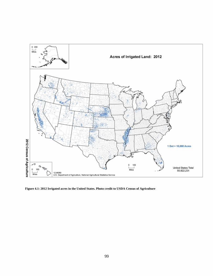
99
Figure 4.1: 2012 Irrigated acres in the United States. Photo credit to USDA Census of Agriculture

100
Figure 4.2: Map of 19 NWS Coop stations used in analysis

101
Figure 4.3: Pre and Post Irrigation minimum temperature difference graph. Calculated by subtracting post irrigation
average from pre irrigation average. Averages for all 19 stations shown.

102
Figure 4.4: Pre and Post Irrigation minimum temperature difference maps. Green denotes stations that had significant
increases in June, July, and August minimum temperatures during the post irrigation epoch. Red denotes averages for
the 13 remaining stations

103
Figure 4.5: Pre and post irrigation dew point temperatures for all 19 stations

104
Figure 4.6: Pre and Post Irrigation dew point temperature difference maps. Green denotes stations that had significant
increases in June, July, and August dew point temperatures during the post irrigation epoch. Red denotes averages for
the 13 remaining stations

105
Figure 4.7: Pre and post irrigation maximum temperature difference for all 19 stations.

106
Figure 4.8: Pre and post irrigation precipitation difference for all 19 stations.

107
Figure 4.9: Map showing location of Albany NWS Coop station (green circle). The red circles represent mapped center
pivot irrigation (CPI) systems for 2008.

108
Figure 4.10: Albany, GA pre and post irrigation difference graphs for precipitation (upper left), minimum temperature
(upper right), maximum temperature (lower left), and dew point temperatures (lower right). Blue represents the pre-
irrigation averages minus the 1938-2013 period of record (P.O.R.). Red represents post irrigation minus P.O.R. and green
represents post irrigation minus pre irrigation values.
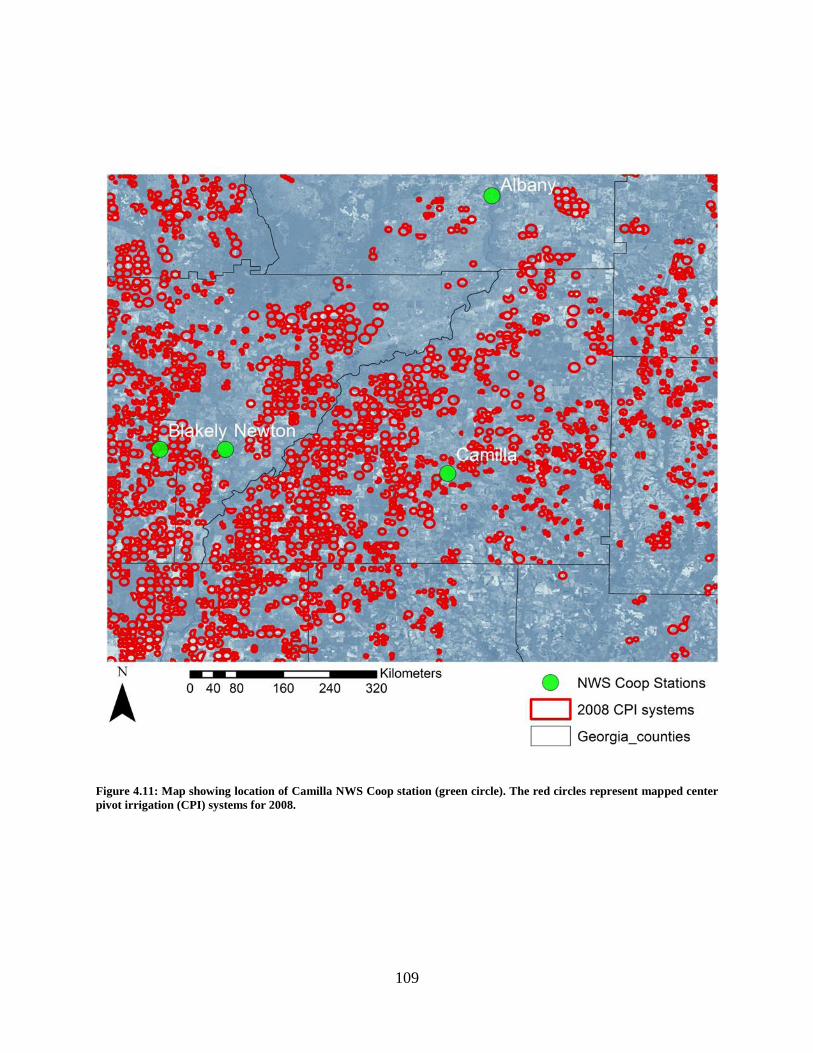
109
Figure 4.11: Map showing location of Camilla NWS Coop station (green circle). The red circles represent mapped center
pivot irrigation (CPI) systems for 2008.
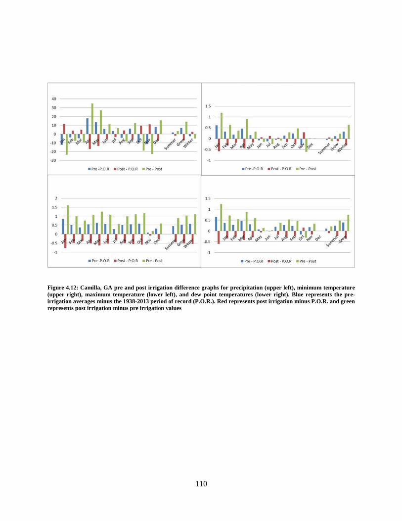
110
Figure 4.12: Camilla, GA pre and post irrigation difference graphs for precipitation (upper left), minimum temperature
(upper right), maximum temperature (lower left), and dew point temperatures (lower right). Blue represents the pre-
irrigation averages minus the 1938-2013 period of record (P.O.R.). Red represents post irrigation minus P.O.R. and green
represents post irrigation minus pre irrigation values

111
Figure 4.13: Map of HYSPLIT back trajectory calculations for Alma, GA. Black and blue asterisks represent trajectory
calculations for July 1st and 2nd respectively. Red represents the mapped CPI systems in 2008.

112
Figure 4.14: Wind Rose diagram for Alma, GA

113
Figure 4.15: Map showing location of Colquitt NWS Coop station (green circle). The red circles represent mapped center
pivot irrigation (CPI) systems for 2008.

114
5) ON THE IMPACT OF IRRIGATION ON SUMMERTIME SURFACE FLUXES
AND PRECIPITATION IN SOUTHWEST GEORGIA: A MODEL SENSITIVITY
APPROACH
Abstract
There is substantial evidence that irrigation alters the hydrologic cycle and the surface energy
budgets. Since the early 1970s, southwest Georgia has experience rapid growth in acres
artificially irrigated. There is limited understanding on the impacts on this land cover change on
the hydroclimate in the region. Long-term observations are sparse in southwest Georgia, so a
modeling approach is useful to investigate these potential changes. The Weather Research and
Forecasting (WRF) model is employed to simulate relative differences between unirrigated and
irrigated land cover scenarios. Sensitivity experiments of this nature are prevalent in the
literature, as a modeling approach removes potential confounding factors and allows for the
exploration of physical differences that occur when the land cover transitions from unirrigated to
irrigated agriculture. The differences in land cover amongst the simulations created local
differences as opposed to regional, broad scale differences. Sensible and latent heat fluxes
appeared as high/low couplets in the simulations, and changes in land cover shifted the spatial
occurrence of these high low couplets. Some shifts produced differences in surface fluxes on the
order of 400-500 W/m2. Grid cell maximum accumulated precipitation, or the totaled amount of
precipitation that fell at each grid point, was higher for the irrigated land cover in the two runs
where precipitation occurred.

115
5.1 Introduction and Literature Review
Beginning in the 1970s, Georgia experienced rapid growth in agricultural intensity, as
there was a substantial increase in irrigated acreage from 1970 to 1992 (Tyson and Harrison,
1993). Much of this growth was fueled by the expansion of center pivot irrigation technology
and general growth of agriculture in the late seventies (Tyson and Harrison, 1993). The increase
in irrigated acreage continued, although the rate of increase slowed as regulations on agricultural
water withdrawals were put into place by the Georgia Environmental Protection Division (EPD)
in the late 1980s. Agriculture is the largest industry in Georgia and contributed more than $72
billion to the state’s economy in 2015 (Georgia Farm Bureau) with one out of every seven
residents of the state working in agriculture of forest related fields (UGA Cooperative Extension,
2011).
Irrigation is the single largest anthropogenic water use with much of the source of water
for irrigation being derived from groundwater that accounts for over 60% of agricultural water
demands (Braneon and Georgakakos, 2011). Irrigation is highest in the southwest portion of the
state, with minimal amounts of irrigation occurring above the fall line (Tyson and Harrison,
1993) as the Flint, Central, and Coastal regions of Georgia comprise about 95% of crop
production and irrigated acreage (Guerra et al., 2005). During the April – September growing
season irrigation water use is estimated to account for 90% in southwest Georgia (Braneon,
2014) and saw a 1,320% increase in agricultural water withdrawals from 1970 -1990 (Marella et
al, 1990). Competing water demands amongst municipal, industrial, agricultural, and ecological
sectors make water resources and planning challenging for policy makers and stakeholders. A

116
changing climate can also place an additional strain on water resources. It is important to identify
any potential changes to the climate system irrigation poses in the region.
Research has shown that irrigation affects the hydrologic cycle and the surface energy
budget. The impacts on the hydrologic cycle include altering precipitation patterns, modifying
water storage in the atmosphere via increased evapotranspiration, and modifying groundwater
storage through water withdrawals for irrigation (Fig 5.1). Precipitation is often increased
downwind of heavily irrigated areas (Barnston and Schickedanz, 1984; DeAngis et al., 2010;
Harding and Synder, 2012; Pei et al., 2016). Boucher et al. (2004) conducted a set of model
simulations that showed irrigation increases water vapor concentrations in the lower levels of the
atmosphere, and resulted in a significant cooling of 0.8K over irrigated continental regions. The
primary impact of irrigation on the surface energy budget is the modification of the Bowen ratio,
which is the partitioning of incoming solar radiation between latent and sensible heating (Fig
5.2). Through the introduction of moisture at the surface, irrigation increases surface
evapotranspiration and near surface humidity; which can lead to changes in the planetary
boundary layer (Qian and Huang et al., 2012). Modeling and empirical studies in various regions
have demonstrated that soil moisture from irrigation leads to decreases in simulated average and
maximum temperatures (Adegoke et al., 2003).
The relationship between irrigation and climate in Georgia has not been as widely studied
as other regions. The literature is more robust on the hydrologic impacts of irrigation in Georgia
as it has been shown that irrigation impacts groundwater resources and streamflows (Braneon
2014, Hicks and Golladay 2009; Mitra et al., 2016; Rugel et al., 2011). In one of the few studies

117
to investigate the climatic response to irrigation in Georgia Misra et al. (2012) found that
irrigation had a meaningful impact on summer minimum and maximum temperature trends.
Their analysis showed than maximum temperatures cooled by 0.5°F per century and that
minimum temperatures increased by 3.5°F per century. There is evidence that irrigation
influences climate in Georgia, but the lack of quality long term meteorological observations
make it difficult to quantify the relationship. Therefore, a modeling approach would serve as a
theoretical foundation to broaden the knowledge of the relationship between irrigation and
climate in Georgia.
This analysis investigates the relative differences between non irrigated and irrigated land
cover. The questions of interest are: (1) can irrigation modify surface latent and sensible heat
fluxes; and (2) are there any spatial differences in precipitation patterns between irrigated and
unirrigated land surfaces. Model simulations are a widely recognized approach to answer the
hypothesized questions. Models allow for a controlled environment that remove confounding
factors that often exist in empirical analysis. The only changes in this experiment are to the land
cover type, as both simulations share the meteorological input used to initiate the model run. The
analysis investigates the relative differences amongst the land surfaces and is not an attempt to
simulate realistic forecasts. This theoretical approach is a first step in gaining an understanding
of the effects of irrigation on the regional hydroclimate.
5.2 Methodology
Two distinct land cover scenarios were used as the foundation for the sensitivity
experiments. The first scenario, NO IRRIGATION (NO-IRR), represents land cover based on

118
the United States Geological Survey (USGS) 24-class land use classification implemented in
WRF (Table 5.1). This scenario represents the dominant land cover in the region before rapid
irrigation occurred prior to the mid-1970s (Fig 5.3).The second scenario, IRRIGATION (IRR),
represents the likely land cover after the rapid expansion of irrigation in Georgia. Williams et al.
(2016) provided an assessment of irrigation changes in the region and found substantial increases
in acres irrigated. The increased irrigated acreage was converted from existing non-irrigated
agriculture. For the IRR (Fig 5.4), the dryland, cropland and pasture is replaced with ‘irrigated
cropland and pasture’ to represent the transition to artificial irrigation in the region, as identified
by Williams et al. (2016), and a closer depiction of the current land cover. The soil moisture
availability parameter was changed from .5 to .8, to represent a value closer to saturation. A
simulation for each land cover is conducted for duration of 36 hours. The three periods for the
simulation which are June 29th-30th, July 10th-11th, and July 17th-18th during the 2014
summer. These days were selected because they represent days of moderate and light
precipitation in the domain. In the created difference maps, the IRR field is subtracted from the
NO-IRR field. If a positive difference is referenced, it implies that NO-IRR modeled output is
greater that IRR modeled output for the time or times being referenced. Table 5.1 provides
information on the differences in model surface parameters
WRF and Model Configuration
The Weather and Research and Forecasting (WRF) model (Shamrock et al., 2008) is a
numerical weather prediction (NWP) and atmospheric simulation system designed for both
research and operational applications. It is a compressible, non-hydrostatic, Euler equation,

119
mesoscale meteorological model. WRF features multiple dynamical cores (ARW, NMM), a 3-
dimensional variational (3DVAR) data assimilation and portable code that is efficient in
computing environments ranging from parallel supercomputers to laptops. This study uses the
Advanced Research WRF (ARW) core version of WRF.
The simulations used three nested domains (Fig 5.5), D1, D2, and D3 with horizontal grid
resolutions of 15 km, 5 km, and 1 km, respectively. The largest domain, D1, covers most of the
Southeastern United States and includes parts of the Atlantic and Gulf of Mexico water bodies.
The second domain contains the entire states of Alabama, Georgia, and South Carolina as well as
portions of Mississippi, Tennessee, North Carolina, and Florida. This domain also covers
portions of the Atlantic and Gulf of Mexico. The innermost domain, D3, covers the southwest
portion of the Georgia Coastal Plain. The model uses 30 vertical levels, with the top set at 100
hPa, and 4 soil levels.
The basic atmospheric packages used in all cases were Kain-Fritsch for cumulus cloud
parameterization and WRF single-moment class 3 microphysics. The innermost domain
explicitly resolves precipitation; therefore no cumulus cloud parameterization was needed. Table
1 provides additional information on the configuration of the WRF model. All scenarios are
initialized with the North American Regional Reanalysis (NARR) dataset (Mesinger et al.,
2006), which has a horizontal resolution of 32 km.

120
5.3 Results and Analyses
Sensible and Latent Heat Flux
The simulation for June 30th, 2014 is initialized at 12z on June 29th. The results herein
are discussed in the context of D3, the domain where the land cover changes were made. The
first 12 hours of the model run are used for spin up and disregarded in the analysis. The spatial
distribution of sensible heat flux for the NO-IRR (Fig 5.6.), and IRR (Fig 5.6) simulations 12 h
into the simulation are shown in Figure 5.6. The fluxes in both simulations have initial
differences roughly around 70 W/m2 (Fig 5.6). As radiative energy from the sun decreases, the
differences in sensible heat flux between the surfaces begin to dissipate, and differences reach a
minimum around 10z on June 30th. At 14z, a few hours after sunrise, differences between the
two surfaces develop in the eastern portion of D3. Sensible and latent heat fluxes were plotted
for the two runs at a grid cell near 31.5N and -83.0W (Figure 5.7). Latent heat fluxes during the
day were higher than sensible heat fluxes in IRR and NO-IRR simulations. Precipitation could be
influencing the fluxes. Peak latent heat flux value occurred at 18z for both simulations, with a
higher peak of approximately 30 W/m2. At the 18z simulation time, many localized differences
in latent heat flux began to develop between the NO-IRR and IRR simulations. The differences
in available soil moisture, albedo, and surface roughness between the two land cover scenarios
do not appear great enough to produce large scale differences in sensible heat flux at the scale of
this study. An emerging pattern of a shift in local minimum and maximum fluxes between the
two scenarios begins to materialize on this day. It appears that there are not any large changes in
the value amongst latent heat fluxes, but spatial differences on where these minimum and

121
maximum values occur begin to create large local differences between the two simulations.
These differences can represent areas of rising air, called thermals. Thermals indicate the
development of shallow cumulus clouds. Spatial changes in areas of maximum sensible heat flux
could lead to spatial changes where cumulus clouds develop. An example of this is seen in the
20z sensible heat plots (Fig 5.8). In the lower right corner of the domain, NO-IRR run has a local
maximum latent heat flux of 470 W/m2. This local maximum is located in Coffee, county
Georgia (approx. 31°30’N & 83°W) and is surrounded by areas of very low sensible heat flux.
The local maximum in latent heat flux is shifted south in the IRR simulation and is slightly
higher, 497 Wm2. If subtracted directly, this would only result in a small difference in sensible
heat flux. The spatial shift in local maximum between the two scenarios creates a positive
difference of 462 W/m2 and a decrease of 501 W/m
2. It is possible that the differences in latent
heat flux can modify precipitation or local cloud cover. At the 21z simulation time latent and
sensible heat fluxes sharply decline in the NO-IRR run (Fig 5.7). Values remain higher in the
IRR run at 21z as the latent heat flux is 281 W/m2 higher and the latent heat flux is greater by
131 W/m2. This could indicate the presence of clouds in the NO-IRR run that are not present in
the IRR run.
The simulation on June 10th
2014 followed a similar pattern as the prior simulation.
Localized differences between the two scenarios began to develop around 12z for this day and
again, the greatest differences were in the eastern portion of the domain. The largest differences
in sensible heat flux occurred at 18z in Coffee County, and the surrounding counties of Bacon
and Jeff Davis. The northwest quadrant of the domain also began to develop flux difference

122
couplets at 18z (Fig 5.9). The July 17th
– 18th
simulation was a relatively dry day. This day yields
interesting results as the differences in fluxes for this simulation closely follow the spatial pattern
of where the land cover was converted from unirrigated agriculture to irrigated agriculture, as
shown in figure. The 18z time frame illustrates the point well (Fig 5.10). Differences in latent
heating resembled the general spatial pattern displayed by sensible heating, with the sign of the
difference between changing direction as expected. The high/low flux couplets in latent heating
were not as large spatially as they were in sensible heating.
Precipitation
There was a marginal amount of precipitation in the July 17-18th
simulation so the results
of those simulations are not discussed here. For the remaining simulations the differences in
daily totals are presented. Figure 5.11 shows that the model produces precipitation that was
observed on June 29th
. On both days, there appears to a shift in daily maximum values of
precipitation. Like the pattern shown in sensible and latent heating, there are some
increase/decrease couplets which signal a shift in where the maximum amount of precipitation is
located. Coffee County, an area of large latent heat differences, displayed a decline in total
precipitation in the IRR simulation (Fig 5.12). The June 29-30th domain total cumulative
precipitation amounts were 72,139.5 mm for the NO-IRR simulation compared to 70,347.9 mm
for the IRR simulation. Despite producing higher total precipitation values, the IRR simulation
produced the highest daily precipitation amount at 41.46 mm compared to 35.82 mm for the NO-
IRR run. There is an area in the upper right quadrant of the domain were total precipitation
increased by more than a 25 mm during the IRR simulation. Most changes are confined to the

123
upper right quadrant on the June 29th
-30th
simulation. Precipitation is more widespread during
the July 10th
-11th
simulation (Fig 5.13). The domain total cumulative precipitation in this
simulation was higher for the IRR run. A total of 178,285 mm of precipitation fell in the IRR run
compared to 155,662 mm in the NO-IRR run. The IRR run produced the highest grid cell
maximum cumulative precipitation, an amount of 68.77 compared to 63.64 for the NO-IRR run.
The additional soil moisture associated with the IRR simulations appears to increase storm total
precipitation amounts.
5.4 Summary
It was clearly shown that there were relative differences in sensible and latent heat flux and
precipitation between the NO-IRR and IRR simulations, which is in agreement with the results
of similar studies. The duration and scale of the simulations did not allow for a full quantification
enhancing precipitation downwind, but the local shifts in precipitation that were found could lead
to enhanced downwind precipitation over time. The meteorological conditions were the same for
both simulations, with the only differences occurring in the land cover. The differences in
albedo, surface roughness, and available soil moisture between the two land cover scenarios did
not appear to create any large scale differences during the three 36 h simulations. The differences
between the scenarios were localized. Although the changes appear to be local; it is reasonable to
assume these changes found between the two land cover types increase over longer simulations.
The differences in latent and sensible heat flux appear to occur in areas where unirrigated and
irrigated land cover bordered other land cover types, such as forested land cover. Coffee County

124
is an example of this mixed land cover scenario. The differences between the two simulations
appeared to occur in high/low couplets, which implies that the differences in the land cover types
created a shift in local minimum and maximum values of fluxes and precipitation rather than
changed the magnitude of the fluxes and precipitation totals. This shift can be the difference of a
surplus of rain at a farm or a summer of little or no rain. In the two simulations where moderate
rainfall was produced, the grid cell maximum accumulated precipitation was higher for IRR
runs. A natural logical next step in future research is to see if these differences manifest
themselves over larger spatial scales during longer simulations.
5.5 References
State and Private Forestry Fact Sheet: Georgia 2016. (2016, February 2). Retrieved May 20,
2016, from http://www.stateforesters.org/sites/default/files/publication-
documents/GAFY2016Standard.pdf
Adegoke, J. O., Pielke, R. A., Eastman, J., Mahmood, R., & Hubbard, K. G. (2003). Impact of
Irrigation on Midsummer Surface Fluxes and Temperature under Dry Synoptic
Conditions: A Regional Atmospheric Model Study of the U.S. High Plains. Mon. Wea.
Rev. Monthly Weather Review, 131(3), 556-564. doi:10.1175/1520-
0493(2003)1312.0.co;2
Barnston, A. G., & Schickedanz, P. T. (1984). The Effect of Irrigation on Warm Season
Precipitation in the Southern Great Plains. J. Climate Appl. Meteor. Journal of Climate
and Applied Meteorology, 23(6), 865-888. doi:10.1175/1520-0450(1984)0232.0.co;2
Boucher, O., Myhre, G., & Myhre, A. (2004). Direct human influence of irrigation on

125
atmospheric water vapour and climate. Climate Dynamics, 22(6-7). doi:10.1007/s00382-
004-0402-4
Braneon, C., & Georgakakos, A. (2011). Climate change impacts on Georgia agriculture and
irrigation demand. 2011 Georgia Water Resources Conference (pp. 1-2).
Braneon, C. V. (2014). Agricultural Water Demand Assessment in the Southeast U.S. Under
Climate Change (Doctoral dissertation, Georgia Tech, 2014) (pp. 1-240). Atlanta, GS:
Georgia Institute of Technology.
Deangelis, A., Dominguez, F., Fan, Y., Robock, A., Kustu, M. D., & Robinson, D. (2010).
Evidence of enhanced precipitation due to irrigation over the Great Plains of the United
States. J. Geophys. Res. Journal of Geophysical Research, 115(D15).
doi:10.1029/2010jd013892
Georgia Trend. (2007). The Longleaf Pine: Georgia's First Tree. Retrieved May 21, 2016, from
http://www.georgiatrend.com/April-2007/The-Longleaf-Pine-Georgias-First-Tree/
Guerra, L. C., Garcia y Garcia, A., Hoogenboom, G., Hook, J. E., Harrison, K. A., & Boken, V.
K. (2005). Impact of local weather variability on irrigation water use in Georgia. In 2005
Georgia Water Resources Conference (pp. 1-4). Athens: Institute of Ecology.
Hicks, D. W., & Golladay, S. W. (2009). Impacts of Agricultural pumping on selected streams in
southwest Georgia. J.W. Jones Ecological Research Center, 1-29.
Lobell, D. B., & Bonfils, C. (2008). The Effect of Irrigation on Regional Temperatures: A
Spatial and Temporal Analysis of Trends in California, 1934–2002. Journal of Climate
J. Climate, 21(10), 2063-2071. doi:10.1175/2007jcli1755.1

126
Marella, R. L., Fanning, J. L., & Mooty, W. S. (1990). Estimated Use of Water in the
Apalachicola Chattahoochee-Flint River basin during 1990 with State summaries from
1970 to 1990. Water-Resources Investigations Report 93-4085, 1-45.
Mesinger, F., Dimego, G., Kalney, E., Mitchell, K., Shafran, P. C., Ebisuzaki, W., . . . Shi, W.
(2006). North American Regional Reanalysis. Bulletin of the American Meteorological
Society, 343-360.
Misra, V., Michael, J. P., Chassignet, E. P., Griffin, M., & O'Brein, J. J. (2012). Reconciling the
Spatial Distribution of the Surface Temperature Trends in the Southeastern United
States. Journal of Cliamte, 25, 3610-3618. http://dx.doi.org/10.1175/JCLI-D-11-00170.1
Mitra, S., Srivastava, P., & Singh, S. (2015). Effects of Irrigation Pumpage during Droughts on
Groundwater Levels and Groundwater Budget Components in the Lower Apalachicola-
Chattahoochee-Flint River Basin [Abstract]. ASABE 1st Climate Change Symposium:
Adaptation and Mitigation, 1-4. doi:10.13031/cc.20152143182
Pei, L., Moore, N., Zhong, S., Kendall, A. D., Gao, Z., & Hyndman, D. W. (2016). Effects of
Irrigation on Summer Precipitation over the United States. Journal of Climate J.
Climate, 29(10), 3541-3558. doi:10.1175/jcli-d-15-0337.1
Qian, Y., Huang, M., Yang, B., & Berg, L. K. (2013). A Modeling Study of Irrigation Effects on
Surface Fluxes and Land–Air–Cloud Interactions in the Southern Great Plains. J.
Hydrometeor Journal of Hydrometeorology, 14(3), 700-721. doi:10.1175/jhm-d-12-
0134.1
Rugel, K., Jackson, C. R., Romeis, J. J., Golladay, S. W., Hicks, D. W., & Dowd, J. F. (2011).

127
Effects of irrigation withdrawals on streamflows in a karst environment: Lower Flint
River Basin, Georgia, USA. Hydrol. Process. Hydrological Processes, 26(4), 523-534.
doi:10.1002/hyp.8149
Skamarock, W. C., & Klemp, J. B. (2008). A time-split nonhydrostatic atmospheric model for
weather research and forecasting applications. Journal of Computational Physics,
227(7), 3465-3485. doi:10.1016/j.jcp.2007.01.037
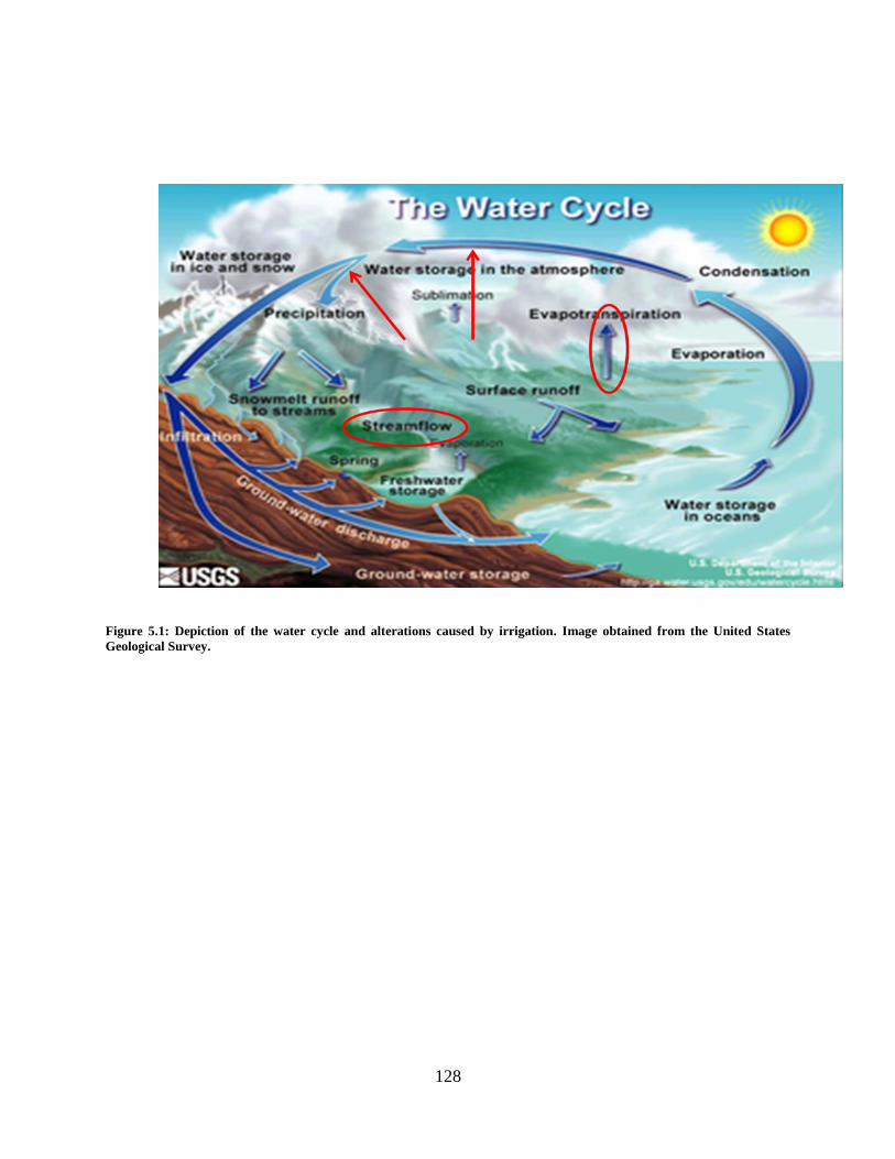
128
Figure 5.1: Depiction of the water cycle and alterations caused by irrigation. Image obtained from the United States
Geological Survey.
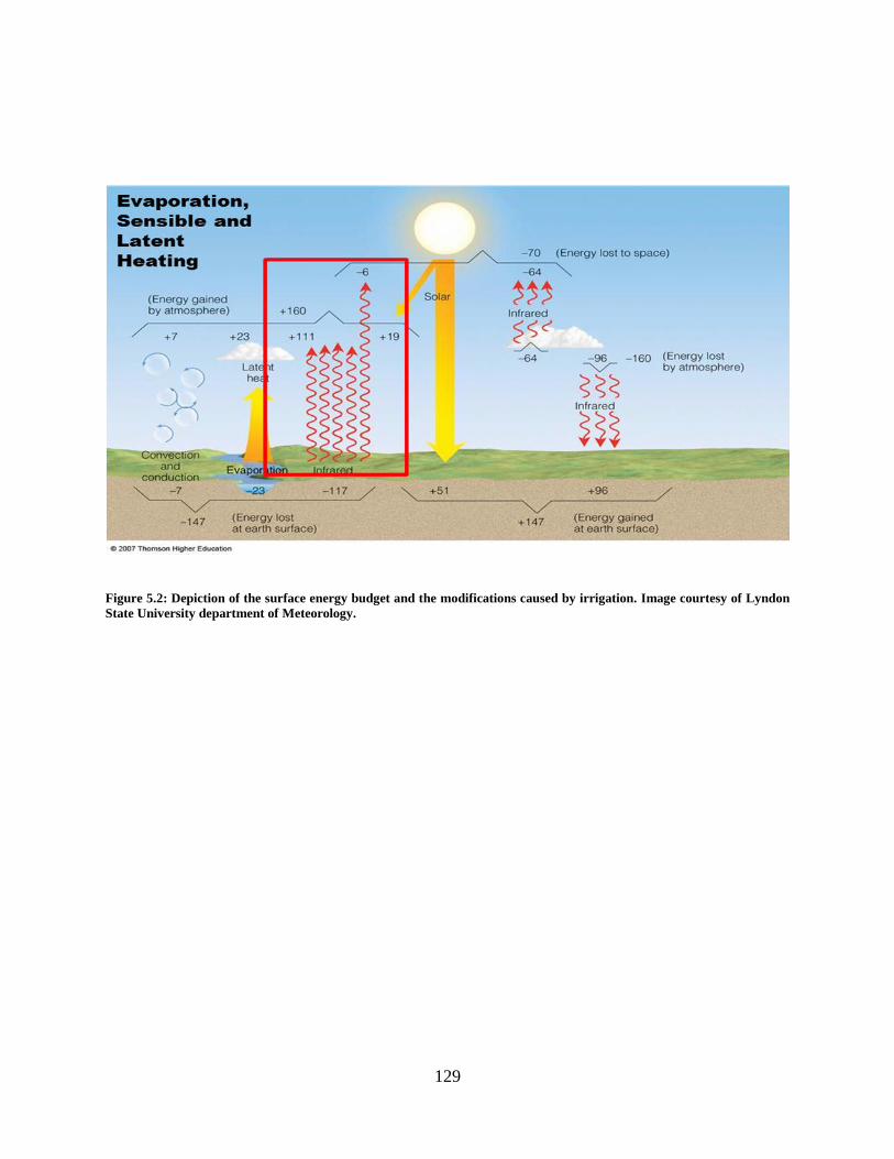
129
Figure 5.2: Depiction of the surface energy budget and the modifications caused by irrigation. Image courtesy of Lyndon
State University department of Meteorology.

130
Land Use Category Land Use Description
1 Urban and Built-up Land
2 Dryland Cropland and Pasture
3 Irrigated Cropland and Pasture
4 Mixed Dryland/Irrigated Cropland and Pasture
5 Cropland/Grassland Mosaic
6 Cropland/Woodland Mosaic
7 Grassland
8 Shrubland
9 Mixed Shrubland/Grassland
10 Savanna
11 Deciduous Broadleaf Forest
12 Deciduous Needleleaf Forest
13 Evergreen Broadleaf
14 Evergreen Needleleaf
15 Mixed Forest
16 Water Bodies
17 Herbaceous Wetland
18 Wooden Wetland
19 Barren or Sparsely Vegetated
20 Herbaceous Tundra
21 Wooded Tundra
22 Mixed Tundra
23 Bare Ground Tundra
24 Snow or Ice Table 5-1: 24-class land use classification used in the WRF simulations derived from USGS.

131
Figure 5.3: Land use category for NO-IRR model simulations.

132
Figure 5.4: Land use category for IRR model simulations.

133
Figure 5.5: Image of model domain set up. Largest domain D1 has a horizontal resolution of 15km, medium domain D2
has a horizontal resolution of 5km, and innermost domain D3 has a horizontal resolution of 1km.
Table 5-2: Table showing land surface parameters for the NO-IRR and IRR model simulations.

134
Figure 5.6: June 30th sensible heat flux for a) NO-IRR, b) IRR, and c) the differences in sensible heat flux between the
two simulations.
Figure 5.7: Sensible and Latent heat flux for NO-IRR and IRR simulations. Plots are for grid point near 31.5N and -
83.5W (Coffee County). Blue and yellow lines represent NO-IRR latent and sensible heat fluxes respectively. Red and
grey lines represent IRR latent and sensible heat fluxes, respectively.

135
Figure 5.8: 20z June 30 sensible heat flux for a) NO-IRR, b) IRR, and c) the difference in flux between the two surfaces.
Figure 5.9: 18z July 11th differences in latent heat flux between NO-IRR and IRR simulations (W/m2).

136
Figure 5.10: Sensible heat flux for 18z July 18th 2014 (W/m2).

137
Figure 5.11: Image showing observed 24-hr precipitation on left hand side and model accumulated precipitation on June
30th, 2014. Obeserved precipitation photo credit to NCEP
(http://www.wpc.ncep.noaa.gov/dailywxmap/index_20140630.html)
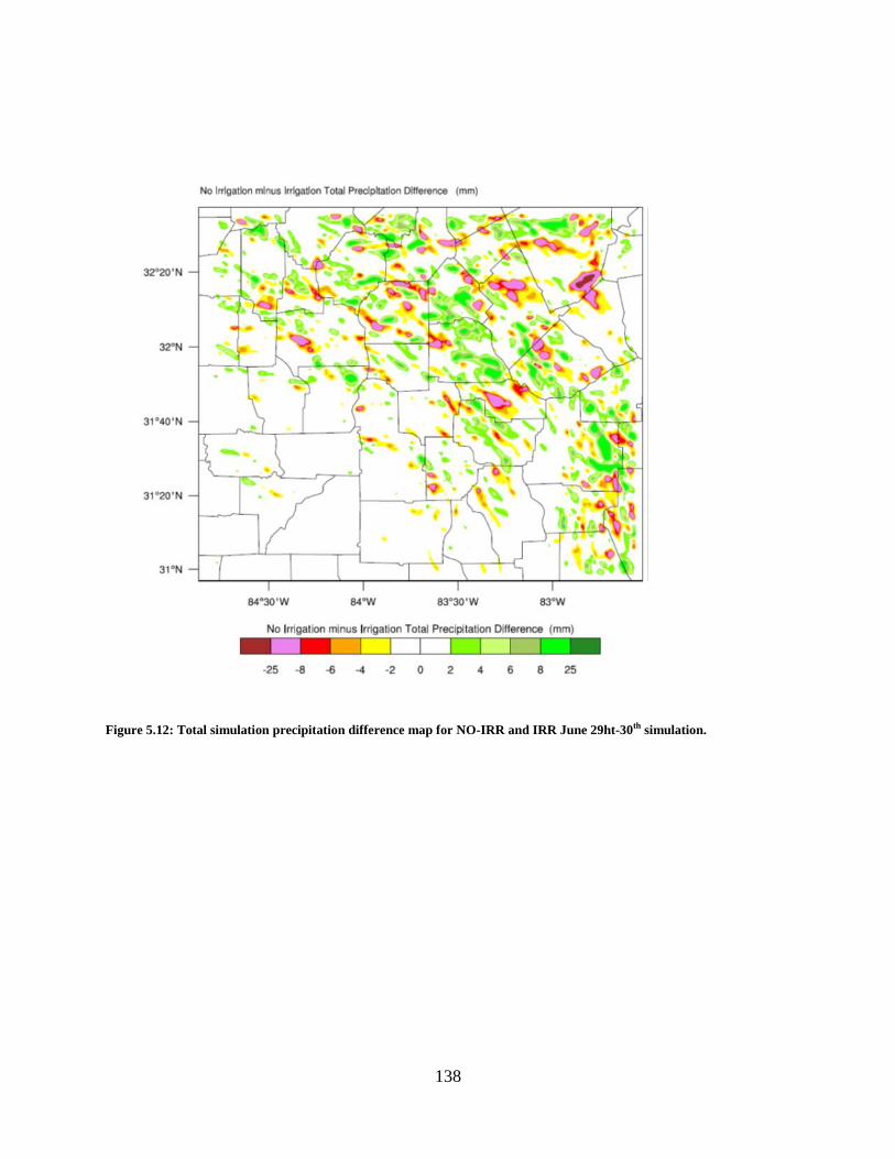
138
Figure 5.12: Total simulation precipitation difference map for NO-IRR and IRR June 29ht-30th simulation.

139
Figure 5.13: Total simulation precipitation difference map for NO-IRR and IRR July 10th-11th simulation.

140
6) SUMMARY AND CONCLUSIONS
6.1 Overview
Georgia has a humid subtropical climate, and climates of this type are generally perceived
to have minimal irrigation needs. However, the increasingly sporadic nature of summertime and
growing season precipitation in the region has made irrigation an attractive and more reliable
alternative to relying on precipitation for agricultural crop production. Georgia has experienced
rapid growth in irrigated acreage since the 1970s and the irrigated acreage continues to grow in
the region. Evidence suggests that the increased irrigation often results in a net loss of water in
irrigated areas, thus creating a positive feedback that strengthens the need to irrigate. Competing
water use needs among private, municipal, and agricultural industries exacerbates the need to
understand the impact of irrigation on the climate in Georgia.
This study addresses the need for a better understanding of the role of irrigation in
Georgia’s past and current climate. The objectives of this dissertation are to map the spatial and
temporal development of irrigation in Georgia (Chapter 2). Chapter 3 addresses the limited
availability to analyze long term changes in humidity by creating an adequate dew point
temperature estimation method, tailored specifically for Georgia. Chapter 4 applies this method
to assess the pre- and post-irrigation differences in climate. Chapter 5 uses the WRF model to
address the climatic impact of transitioning from unirrigated agriculture to irrigated agriculture.

141
6.2 Conclusions
The findings from this dissertation extend existing knowledge on the impact of irrigation
on climate and provide new perspectives that have been sparsely represented for the
Southeastern U.S., particularly within the Coastal Plains region of Georgia. The results indicate
that Georgia has experienced rapid growth in irrigated acreage since the mid-1970s. An analysis
of remotely sensed data spanning 38 years (1976-2013) revealed a 4,500% increase in Center
Pivot Irrigation (CPI) systems that corresponded to an approximate 2,000% increase in total area
of CPI-irrigated land. The bulk of the total acreage irrigated is located in southwest Georgia, as
seven counties in the region contained 38% of the total acreage irrigated in 2013. One of the first
mapped time series of irrigated acreage in Georgia was created as a result of this analysis.
To assess long-term changes in moisture in the region, it was critical to analyze long-term
dew point temperatures. The lack of long-term daily average dew temperatures created the need
for the development of an adequate estimation method. Dew point temperatures were estimated
and evaluated at 14 NWS Coop stations in southwest Georgia using linear regression models and
artificial neural network (ANN) analysis. Estimation methods were drawn from simple and
readily available meteorological observations, therefore only temperature and precipitation were
considered as input variables. Both methods produced adequate estimates of daily averaged dew
point temperatures with the ANN displaying the best overall skill. On average, the ANN reduced
root mean square error (RMSE) by 6.86% and mean absolute error (MAE) by 8.30% when
compared to the best performing linear regression model. The ability to assess long-term changes

142
in dew point temperature in areas outside of first order stations was also a by-product of the work
performed in this dissertation.
In an era defined as post-irrigation since the installation of artificial irrigation structures
such as center pivot irrigation (CPI) in the mind 1970s in the Georgia Coastal Plain, empirical
analysis suggests that increased irrigation has modified summer humidity and temperatures. A
total of 19 stations in the Georgia Coastal Plain were analyzed to determine differences in the
hydroclimate in pre-irrigation and post-irrigation epochs. Analysis found that summer minimum
and dew point temperatures were most impacted. Precipitation was most impacted in April and
November. Further research is needed to determine if or how the changes in precipitation are
influenced by irrigation. The poor data quality in the region made it difficult to isolate the impact
of irrigation as many stations had multiple years of missing data. There were also confounding
factors that make it difficult to isolate the impact of irrigation empirically. To limit the influence
of poor data quality and confounding factors created by the microclimate of each observation
station, this analysis was extended via a modeling approach.
To investigate the relative differences between non-irrigated and irrigated land cover
scenarios, three 36h model simulations were conducted using version 3.5 of the WRF Model.
The case study analysis showed that the differences in land cover created spatial shifts in latent
and sensible heat fluxes. The irrigated land cover had higher sensible and latent heat fluxes for
all three case studies and produced higher grid cell maximum accumulated precipitation. The
increase in near surface moisture impacts where local minimum and maximum fluxes occur and
this local shift impacts local development of convection.
143
Agriculture is the largest industry in Georgia and its continued growth and maintenance is
vital to the state’s economy. Combined with climate changes and recent transitions in the types
of crops produced in Southwest Georgia, continued increases in artificial irrigation are expected.
With the expected continuing reliance on irrigation, it is of utmost important to continue to
monitor and map irrigation in the region beyond this study. The research presented here suggests
that irrigation has impacted the hydroclimate in Georgia, and this relationship is expected to
strengthen as irrigated acreage increases in the future. The greatest impacts of irrigation in the
state are local, but the cumulative impacts have already begun to cause larger problems. Results
shown here suggest that minimum and dew point temperatures were impacted the most, which is
in agreement with other studies of this nature. Other studies have also noted that irrigation causes
a reduction in summer maximum temperatures, but that result was not as conclusive in the
Georgia Coastal Plain. Early growing season and summer precipitation decreased during the
more intensely irrigated time period, but further research must be conducted before directly
attributing this decrease to irrigation. One issue that arose was the lack of complete and
consistent long term climate observations in the region. Improvements in data quality can
provide a better context on the long term impacts of irrigation discussed in this study
The ongoing dispute between Alabama, Florida, and Georgia known as the “Tri-State
Water Wars” provides an example of the wide reaching impacts of irrigation within Georgia. The
dispute began over allocation of water resources in the Alabama-Coosa-Tallapoosa (ACT) and
Apalachicola-Chattahoochee-Flint (ACF) river basins. Irrigation density and water withdrawals
are highest in the Lower Flint basin in Georgia. This removal of water upstream has reduced the

144
water reaching Florida, and has negatively impacted Florida’s multi-million dollar shellfish
industry. Results found here provide evidence that increased near surface moisture caused by
irrigation has resulted in a net loss of water in the region. The net water loss strengthens the need
to irrigate in the future. This reliance on irrigation can potentially create a positive feedback and
introduce wide reaching negative ecological and economic impacts as seen in the Tri-State Water
Wars.