Embed Size (px)
Citation preview
Long-Distance Quantum Key Distribution over Telecom
Fiber
by
Lei-Lei Huang
A thesis submitted in conformity with the requirementsfor the degree of Master of Applied Science
Graduate Department of Electrical & Computer EngineeringUniversity of Toronto
Copyright c© 2006 by Lei-Lei Huang
Abstract
Long-Distance Quantum Key Distribution over Telecom Fiber
Lei-Lei Huang
Master of Applied Science
Graduate Department of Electrical & Computer Engineering
University of Toronto
2006
We present two long-distance quantum key distribution (QKD) systems over telecom
fiber. The first one is the Sagnac QKD system implementing standard BB84 protocol.
Novel polarization-insensitive phase modulators are used to simplify the conventional ar-
chitecture. We are able to achieve a stable quantum bit error rate of 4-6.5% over 40km
fiber loop over one hour without recalibration. The second one is the fiber-based QKD
system using Gaussian-modulated coherent states. We have overcome the challenges im-
posed by the requirements for high detector sensitivity, long-term stability, and low signal
crosstalk. Our GMCS QKD system is the first practical fiber-based one-way demonstra-
tion and is able to achieve a sifted secret key rate of 15.5kbits/s over a transmission
distance of 5km fiber .
Experimental QKD is still in its infancy. The results presented in this thesis represent
a significant step forward towards the practical QKD over conventional fiber networks.
ii
Acknowledgements
I would like to express my sincere gratitude and appreciation to my supervisors,
Professor Li Qian and Professor Hoi-Kwong Lo, for their inspiration, vision, guidance,
availability, and encouragement over the last two years.
I would like to thank Dr. Bing Qi for suggesting creative ideas for experiments and
helping to build experimental setups.
I would like to thank Professor Stewart Aitchison, Professor Peter R. Herman and
Professor Frank Kschischiang for serving on my committee.
I would like to express my thanks to Andrew Tausz, Justin Chan, and Roger Mong,
who were the summer students in the lab. They provided great help to me in the project.
I am grateful to all previous and current members of Professor Li Qian and Professor
Hoi-Kwong Lo’s groups for their indispensable support and valuable friendships.
Above all, I am deeply grateful to my parents for their spiritual support.
iii

Contents
Abstract ii
Acknowledgements iii
List of Figures vii
List of Tables x
1 Introduction 1
1.1 Motivation . . . . . . . . . . . . . . . . . . . . . . . . . . . . . . . . . . . 1
1.1.1 Cryptography . . . . . . . . . . . . . . . . . . . . . . . . . . . . . 1
1.1.2 Quantum Cryptography (QC) . . . . . . . . . . . . . . . . . . . . 3
1.1.3 Challenges in Experimental QC . . . . . . . . . . . . . . . . . . . 4
1.2 Objectives . . . . . . . . . . . . . . . . . . . . . . . . . . . . . . . . . . . 5
1.3 Organization of Thesis . . . . . . . . . . . . . . . . . . . . . . . . . . . . 6
2 Quantum Key Distribution (QKD) 7
2.1 QKD Protocol and Implementation . . . . . . . . . . . . . . . . . . . . . 7
2.1.1 Single Photon QKD . . . . . . . . . . . . . . . . . . . . . . . . . 7
2.1.2 Continuous Variables QKD . . . . . . . . . . . . . . . . . . . . . 14
2.2 State of the Art . . . . . . . . . . . . . . . . . . . . . . . . . . . . . . . . 19
2.3 Summary . . . . . . . . . . . . . . . . . . . . . . . . . . . . . . . . . . . 20
iv
3 Sagnac QKD with Polarization-insensitive Phase Modulators 21
3.1 Introduction . . . . . . . . . . . . . . . . . . . . . . . . . . . . . . . . . . 21
3.2 Polarization-insensitive Phase Modulators . . . . . . . . . . . . . . . . . 22
3.3 Sagnac QKD System . . . . . . . . . . . . . . . . . . . . . . . . . . . . . 26
3.3.1 Experimental Setup . . . . . . . . . . . . . . . . . . . . . . . . . . 26
3.3.2 Synchronization . . . . . . . . . . . . . . . . . . . . . . . . . . . . 29
3.4 Experimental Results . . . . . . . . . . . . . . . . . . . . . . . . . . . . . 30
3.5 Summary . . . . . . . . . . . . . . . . . . . . . . . . . . . . . . . . . . . 34
4 Gaussian-modulated Coherent States (GMCS) QKD System Design 37
4.1 System Design . . . . . . . . . . . . . . . . . . . . . . . . . . . . . . . . . 37
4.2 Homodyne Detection Design . . . . . . . . . . . . . . . . . . . . . . . . . 39
4.2.1 Electrical Amplifier . . . . . . . . . . . . . . . . . . . . . . . . . . 43
4.2.2 Optical Balancing . . . . . . . . . . . . . . . . . . . . . . . . . . . 47
4.2.3 Shot Noise Measurement . . . . . . . . . . . . . . . . . . . . . . . 50
4.3 Drift Compensation System . . . . . . . . . . . . . . . . . . . . . . . . . 54
4.3.1 Phase Drift . . . . . . . . . . . . . . . . . . . . . . . . . . . . . . 54
4.3.2 Polarization Drift . . . . . . . . . . . . . . . . . . . . . . . . . . . 59
4.4 Frequency-multiplexing . . . . . . . . . . . . . . . . . . . . . . . . . . . . 59
4.5 Initialization Procedure . . . . . . . . . . . . . . . . . . . . . . . . . . . . 62
4.6 Experimental Procedure . . . . . . . . . . . . . . . . . . . . . . . . . . . 63
4.7 Summary . . . . . . . . . . . . . . . . . . . . . . . . . . . . . . . . . . . 65
5 Gaussian-modulated Coherent States QKD System Results 66
5.1 System Results . . . . . . . . . . . . . . . . . . . . . . . . . . . . . . . . 66
5.2 Summary . . . . . . . . . . . . . . . . . . . . . . . . . . . . . . . . . . . 71
6 Conclusions 74
6.1 Contributions . . . . . . . . . . . . . . . . . . . . . . . . . . . . . . . . . 74
v
6.2 Future Work . . . . . . . . . . . . . . . . . . . . . . . . . . . . . . . . . . 77
6.2.1 Sagnac Loop QKD System . . . . . . . . . . . . . . . . . . . . . . 77
6.2.2 GMCS QKD System . . . . . . . . . . . . . . . . . . . . . . . . . 78
6.3 Summary . . . . . . . . . . . . . . . . . . . . . . . . . . . . . . . . . . . 79
A Gaussian distribution random number generation 80
A.1 Quantum Random Number Generator . . . . . . . . . . . . . . . . . . . 80
A.2 Gaussian distribution . . . . . . . . . . . . . . . . . . . . . . . . . . . . . 81
A.3 Amplitude and phase modulation . . . . . . . . . . . . . . . . . . . . . . 82
Bibliography 83
vi

List of Figures
2.1 BB84 phase coding QKD setup . . . . . . . . . . . . . . . . . . . . . . . 8
2.2 Asymmetric Mach-Zehnder implementation in QKD system . . . . . . . 11
2.3 An example of the plug &play system employing a Faraday mirror . . . . 13
2.4 Sagnac QKD setup . . . . . . . . . . . . . . . . . . . . . . . . . . . . . . 13
2.5 Schematics of the GMCS QKD system . . . . . . . . . . . . . . . . . . . 15
2.6 Schematics of the beam-splitting attack . . . . . . . . . . . . . . . . . . . 17
2.7 Ideal key rate ∆I as a function of the channel transmission G . . . . . . 18
3.1 Schematics of the polarization-insensitive phase modulation . . . . . . . . 23
3.2 Polarization-insensitive phase modulator based on a pair of AOMs . . . . 25
3.3 Optical Sagnac QKD setup . . . . . . . . . . . . . . . . . . . . . . . . . . 26
3.4 Experimental Sagnac QKD setup . . . . . . . . . . . . . . . . . . . . . . 27
3.5 The full Sagnac QKD system in laboratory . . . . . . . . . . . . . . . . . 28
3.6 Bob’s synchronization in the Sagnac QKD system . . . . . . . . . . . . . 30
3.7 The visibilities of the Sagnac QKD system . . . . . . . . . . . . . . . . . 32
3.8 Experimental QBER for the Sagnac QKD system . . . . . . . . . . . . . 33
3.9 The optical-ring QKD network based on the Sagnac interferometer . . . . 34
4.1 Initial GMCS configuration . . . . . . . . . . . . . . . . . . . . . . . . . 38
4.2 GMCS QKD system design . . . . . . . . . . . . . . . . . . . . . . . . . 40
4.3 Schematics of the balanced homodyne detection . . . . . . . . . . . . . . 41
vii
4.4 Homodyne detection design . . . . . . . . . . . . . . . . . . . . . . . . . 43
4.5 Electrical amplifier circuit in the balanced homodyne detector . . . . . . 44
4.6 Typical output signal from the balanced homodyne detector . . . . . . . 45
4.7 The frequency response of the electrical amplifier in the balanced homo-
dyne detector . . . . . . . . . . . . . . . . . . . . . . . . . . . . . . . . . 46
4.8 The output signal from the balanced homodyne detector after increasing
the bandwidth . . . . . . . . . . . . . . . . . . . . . . . . . . . . . . . . . 46
4.9 Electronic noise of the electrical amplifier in the balanced homodyne detector 48
4.10 Unbalanced signal output of the balanced homodyne detector due to time
delay . . . . . . . . . . . . . . . . . . . . . . . . . . . . . . . . . . . . . . 50
4.11 Balanced signals of the balanced homodyne detector . . . . . . . . . . . . 51
4.12 The pulsed shot noise of the balanced homodyne detector . . . . . . . . . 52
4.13 Noise measurement of the balanced homodyne detector . . . . . . . . . . 53
4.14 Asymmetric Mach-Zehnder interferometers in the GMCS QKD system . 54
4.15 The drift of the interference output due to the phase drift. . . . . . . . . 55
4.16 Schematics of the active phase feedback control in the GMCS QKD system 57
4.17 The result of the phase feedback control in the GMCS QKD system . . . 58
4.18 Polarization drifts in the GMCS QKD system . . . . . . . . . . . . . . . 60
4.19 Schematics of time-multiplexing in GMCS QKD system . . . . . . . . . . 61
4.20 Schematics of frequency-multiplexing in the GMCS QKD . . . . . . . . . 62
4.21 GMCS QKD system . . . . . . . . . . . . . . . . . . . . . . . . . . . . . 64
5.1 GMCS QKD experimental setup . . . . . . . . . . . . . . . . . . . . . . . 67
5.2 The experimental pulses in GMCS QKD system . . . . . . . . . . . . . . 68
5.3 Alice’s encoding Gaussian distributed random numbers (x and p) . . . . 69
5.4 Bob’s measured x’ and p’ . . . . . . . . . . . . . . . . . . . . . . . . . . . 70
5.5 Alice and Bob’s correlated x and p . . . . . . . . . . . . . . . . . . . . . 72
viii
A.1 Schematics of the quantum random number generator . . . . . . . . . . . 81
ix
List of Tables
2.1 Implementation of BB84 with phase encoding . . . . . . . . . . . . . . . 9
3.1 Experimental Sagnac QKD results . . . . . . . . . . . . . . . . . . . . . . 35
6.1 Experimental Sagnac QKD results . . . . . . . . . . . . . . . . . . . . . . 75
6.2 Experimental GMCS QKD results . . . . . . . . . . . . . . . . . . . . . . 76
x

Chapter 1
Introduction
1.1 Motivation
1.1.1 Cryptography
In today’s information society, cryptography has become one of the main tools for privacy,
trust, access control, electronic payments, corporate security, and countless other fields.
In cryptography, the secret messages are encoded with some additional information -
called the “key”- and can be decoded only with the key.
There are two main classes of cryptosystems, depending on whether the sender (con-
ventionally called Alice) and the receiver (conventionally called Bob) share the same key
[1]. Asymmetrical cryptosystems, also called public-key cryptosystems, use different keys
for message encryption and decryption. The security of the asymmetrical cryptosystems
relies on the computational difficulties in solving certain mathematical problems. The
basic principle is to use one-way functions, that is, use functions f(x) which are easy
to compute given variable x, but difficult to calculate x from f(x). In terms of compu-
tational algorithm, a problem is difficult (or easy) if the computational time grows as
an exponential (or polynomial) function of the input variable. For example, it is easy
to compute 97 ∗ 83 = 8051 but difficult to calculate the prime factors of 8051. If Bob
1

Chapter 1. Introduction 2
chooses 97 as his “private” key, he then calculates and sends the “public” key 8051 to
Alice for encoding. Because it is difficult for people except Bob to calculate the prime
factors of 8051 (especially when it is a very large number instead of 8051), only Bob has
the “private” key and can decode the secret messages. This kind of asymmetrical system,
called RSA [2], developed by Rivest, Shanmir and Adleman in 1978, is still the widely
used.
Asymmetrical cryptosystems are convenient to implement and are still being widely
used. The security of our current internet infrastructure is partially based on asymmet-
rical systems. The typical length of the current RSA key is 1024 bits. Using current
computer technology, it will take hundreds of years to break a code of this length. In
theory, however, it is not absolutely secure and the security will be further weakened
or suppressed by theoretical and technological advances. For instance, the difficulty of
factoring products of two large prime numbers as mentioned above, is vulnerable to
code-breaking algorithms offered by quantum computers [3]. Moreover, the computer
technology is fast advancing and the length of the key may have to be increased dramati-
cally. Security is so important in our society that we should not tolerate the risk brought
by a potential technological breakthrough.
To eliminate such risks, alternative symmetrical cryptosystems are considered. In
symmetrical cryptosystems, Alice and Bob use the same key for encryption and decryp-
tion. If Alice and Bob share the same random key, it has been proven that if the key
length is as long as the message, and if the random key is used only once, the symmet-
rical cryptosystems are unbreakable (“one-time pad” by Shannon [4]). This is the only
provably secure cryptosystem known to date. In spite of its perfect security, the critical
problem of symmetrical systems is the difficulty to distribute random secret keys between
two remote parties. This is what is known as the “key distribution problem”.
Chapter 1. Introduction 3
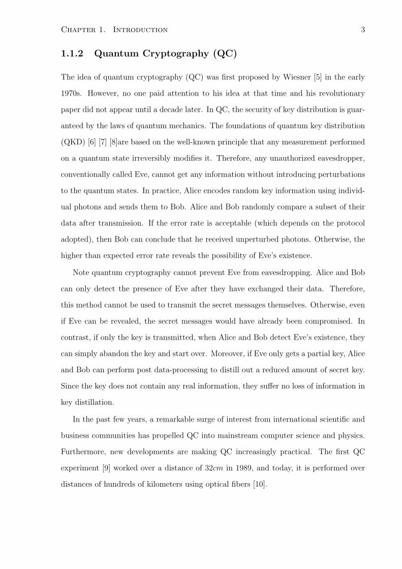
1.1.2 Quantum Cryptography (QC)
The idea of quantum cryptography (QC) was first proposed by Wiesner [5] in the early
1970s. However, no one paid attention to his idea at that time and his revolutionary
paper did not appear until a decade later. In QC, the security of key distribution is guar-
anteed by the laws of quantum mechanics. The foundations of quantum key distribution
(QKD) [6] [7] [8]are based on the well-known principle that any measurement performed
on a quantum state irreversibly modifies it. Therefore, any unauthorized eavesdropper,
conventionally called Eve, cannot get any information without introducing perturbations
to the quantum states. In practice, Alice encodes random key information using individ-
ual photons and sends them to Bob. Alice and Bob randomly compare a subset of their
data after transmission. If the error rate is acceptable (which depends on the protocol
adopted), then Bob can conclude that he received unperturbed photons. Otherwise, the
higher than expected error rate reveals the possibility of Eve’s existence.
Note quantum cryptography cannot prevent Eve from eavesdropping. Alice and Bob
can only detect the presence of Eve after they have exchanged their data. Therefore,
this method cannot be used to transmit the secret messages themselves. Otherwise, even
if Eve can be revealed, the secret messages would have already been compromised. In
contrast, if only the key is transmitted, when Alice and Bob detect Eve’s existence, they
can simply abandon the key and start over. Moreover, if Eve only gets a partial key, Alice
and Bob can perform post data-processing to distill out a reduced amount of secret key.
Since the key does not contain any real information, they suffer no loss of information in
key distillation.
In the past few years, a remarkable surge of interest from international scientific and
business communities has propelled QC into mainstream computer science and physics.
Furthermore, new developments are making QC increasingly practical. The first QC
experiment [9] worked over a distance of 32cm in 1989, and today, it is performed over
distances of hundreds of kilometers using optical fibers [10].

Chapter 1. Introduction 4
Quantum cryptography promises to revolutionize the way we communicate by pro-
viding security based on the fundamental laws of physics, instead of current state of
mathematical algorithms and computing technology. Although it is “quantum”, the de-
vices for implementation, such as sources, channels, detectors, are already commercially
available and most of them are the same as the classical ones. The performance of
demonstrated practical quantum cryptography systems is being continuously improved
at a fast pace. It is safe to say, within the next few years, such systems will be used for
transmitting some of the most valuable secrets of government and industry.
1.1.3 Challenges in Experimental QC
In the past few decades, with the development of electronic and optical telecommunica-
tions, quantum key distribution evolved extraordinarily rapidly. The practical implemen-
tation of quantum communication systems is limited in the key rate and transmission
distance by a number of challenges:
1. The limitation of current component technology. Compared with the classical sys-
tem, since the transmitted data is encoded in a quantum state, a quantum cryp-
tography system is especially sensitive to the quality of the sources, the efficiency
of the detectors, and the quality of channel losses and noises.
2. The efficiency of the protocols. Currently, the quantum communication protocols
do not have as high efficiency as the classical communication protocols. Further
studies are still required to improve the performances of quantum protocols and to
compare the pros and cons of different quantum protocols.
3. The ease of physical implementation. Within the limitation of current component
technologies and protocols, a simple and elegant system can result in a better
system performance than a complicated and inelegant system.
Chapter 1. Introduction 5
1.2 Objectives
The goal of this thesis work is to achieve high performances of quantum cryptographic
systems in realistic environmental settings. In our experiments, a number of efforts have
been made to find novel solutions within the limitation of current technologies. We
generally employ the following two approaches. The first approach is to employ and
implement novel protocols to meet the second challenge, mentioned in Section 1.1.3. A
better protocol, though may not be easy to implement, can greatly improve the system
performance. The second approach is to improve the physical system design to meet the
third challenge, mentioned in Section 1.1.3. A stable and automated system offering a
high performance will be more likely to be adopted in commercial applications.
Our experiments focus on two practical secure quantum cryptography systems over
the commercial fiber. Two different quantum cryptographic systems employing different
protocols have been developed and demonstrated in this thesis, both of which operate
at telecommunication wavelength of 1550nm over conventional fiber communication sys-
tems.
Our research presented here has been carried out with the following objectives:
1. To implement different quantum cryptography protocols and compare their advan-
tage and disadvantages;
2. To provide physical system designs for fiber-based QKD systems;
3. To meet the challenges of experimental QKD implementation and provide innova-
tive solutions;
4. To build, test, and evaluate the performances of the proposed QKD systems and
to outperform the previous demonstrations reported in the literature.
Chapter 1. Introduction 6
1.3 Organization of Thesis
This thesis is organized as follows. Chapter 2 provides the background understanding of
QKD, which is the most important application of current quantum cryptography. The
basic protocols of QKD will be explained and the previous work will be reviewed briefly.
Chapter 3 presents the design and performance of a QKD system using a Sagnac loop
configuration. Our novel design provides an easy implementation and much improved
performance compared with the most recent report on this type of QKD system. Chapter
4 describes the architecture of another QKD system implementing a different protocol -
Gaussian Modulated Coherent States (GMCS). GMCS QKD is a recently proposed pro-
tocol and its full implementation in fiber over a practical transmission distance had never
been demonstrated prior to this work. The many challenges of the GMCS QKD system
are discussed and the corresponding solutions are proposed and implemented. Chapter 5
shows the experimental procedures and characteristics of the GMCS QKD system. The
performance of the GMCS QKD system is analyzed and the data transmission results
are reported. Finally, Chapter 6 summarizes the thesis and suggests topics for future
research.
Chapter 2
Quantum Key Distribution (QKD)
This chapter presents the background of Quantum Key Distribution (QKD). QKD is a
cryptographic process that allows two parties -Alice and Bob- to share a set of random
data (called the “key”), which they can later use to encode their secret messages. Differ-
ent QKD protocols as well as various QKD system architectures are introduced, followed
by the practical design issues and technical challenges in experimental QKD systems.
Finally, because our work focuses on the improvement and demonstration of fiber-based
Sagnac loop and Gaussian-modulated coherent states QKD systems, a brief review of the
relevant work is presented.
2.1 QKD Protocol and Implementation
2.1.1 Single Photon QKD
The first protocol for secure QKD is BB84 [6], named after Bennett and Brassard who
proposed it in 1984. BB84 is a single-photon protocol in the sense that each bit of infor-
mation is encoded using a single photon. BB84 remains the most widely used protocol for
current practical QKD experiments although a number of other single photon protocols
have been proposed in the last few years [8] [11] [12] [13]. A typical system implementing
7

Chapter 2. Quantum Key Distribution (QKD) 8
Figure 2.1: BB84 phase coding QKD setup. PM: phase modulator; SPD: single photon
detector.
BB84 protocol with phase coding is presented in Figure 2.1. It consists of an interferome-
ter with one phase modulator for Alice and one for Bob. If the paths of the interferometer
are equal and the intensity of the laser is reduced to the single-photon level, then the
intensities at the two single photon detectors (SPDs) are: I0 = 12(1 + cos(φA − φB)),
I1 = 12(1 − cos(φA − φB)). Therefore, SPD0 clicks when the phase difference between
signal and reference pulses is 0 (bit 0), and SPD1 clicks when the phase difference is π
(bit 1).
Table 2.1 illustrates the basic implementation of BB84. The protocol uses four quan-
tum states that constitute two non-orthogonal bases: {0, π} (basis“0”) and {π/2, 3π/2}(basis“1”). In basis“0”, {0} represents bit 0, and {π} represents bit 1. In basis“1”, {π/2}represents bit 0, and {3π/2} represents bit 1. In practice, individual photons are used to
transmit bits of quantum information, which is called qubits (quantum bits).
On Alice’s side, Alice uses her single-photon laser source to send out a pulse. She
then uses a phase modulator PMA to randomly apply one of four phase modulations {0,
π/2, π, 3π/2}, which means that she randomly chooses a basis and a bit value to encode.
On Bob’s side, he chooses a basis by randomly applying a phase modulation of either
{0} (basis“0”) or {π/2} (basis“1”) using his phase modulator PMB. When SPD0 clicks,
the resulting value is bit 0, and when SPD1 clicks, it means bit 1.

Chapter 2. Quantum Key Distribution (QKD) 9
Table 2.1: Implementation of BB84 with phase encoding. The grey box in the table
means when Alice and Bob choose the same basis.
After the raw key transmission, Alice and Bob keep their data secret but publicly
compare their bases choices. An example is given in Table 2.1. When Alice and Bob use
compatible bases, they obtain a deterministic result. Consequently, they get correlated
bits. On the other hand, if they choose incompatible bases, Bob has an indeterministic
result, ie., there is 50% probability to get either bit 0 or bit 1. After comparing their
bases, Alice and Bob only retain the data obtained under the compatible bases and drop
the irrelevant data, which means 50% of the data will be discarded on average. Alice and
Bob then publicly compare a random sample of their key elements to evaluate the error
rate and the transmission efficiency. Given the evaluated error rate, for each specific
protocol, Alice and Bob can estimate their mutual information and the information that
is possibly leaked to Eve. They then proceed to data post-processing on their remaining
raw key to extract a set of absolute secure key (a process conventionally known as error
correction and privacy amplification) [14] [15]. If the error rate is higher than a certain
Chapter 2. Quantum Key Distribution (QKD) 10
predetermined value, no secret key can be distilled. In this case, they have to discard
their data and start over.
How can this protocol prevent Eve from successfully getting the key? Here let us
discuss the most intuitive and practical eavesdropping attack, the intercept-and-resend
strategy. If there is an Eve, during data transmission, without any idea of the basis
Alice uses, she measures each qubit in one of the two bases randomly, and resends to
Bob another qubit corresponding to her measurement result. With 50% probability,
Eve chooses the same basis as Alice and will send Bob the correct qubit. In this case,
Alice and Bob will not detect her existence. However, also with 50% probability, Eve
will choose the wrong basis, and will send Bob a qubit in the incompatible basis with
Alice. In this case, even if Bob chooses the compatible basis with Alice, he will get an
indeterministic result, i.e, he will have a result with 50% error rate. Overall, Eve will
introduce 25% error rate if she uses intercept-and-resend strategy to eavesdrop each bit.
Since 25% error rate is high and therefore can be easily detected, Eve can also reduce
the chance of being detected by applying this strategy to only a fraction of the bits. For
example, if Eve uses the intercept-and-resend strategy to only 20% of the transmitted
bits, the error rate will be only 5%, but Eve gets 10% of the information. This 10%
leakage can be filtered out through the privacy amplification process. The security of
this kind of protocol actually relies on the fact that Alice and Bob can take advantage
of which data they want to keep after data transmission, whereas Eve does not have this
control.
It is essential to keep the interference path difference stable during key transmission
as shown in Figure 2.1. If the path length difference changes by more than a fraction of
a wavelength, the relative phase information will be changed. In practice, even if Alice
and Bob are separated by a distance of only a few meters, it is nearly impossible to
keep the path difference stable to within one wavelength. In particular, changes in the
ambient conditions, such as air flow, temperature, etc., cause a drift of the optical path

Chapter 2. Quantum Key Distribution (QKD) 11
Figure 2.2: Asymmetric Mach-Zehnder implementation in QKD system.
length. Consequently, the phase instability will induce additional phase difference and
cause large quantum bit error rate (QBER).
In addition, since the qubits are decoded from the interference signal, the interfer-
ence visibility also will affect the QBER. The QBER contributed by the imperfection of
interferometer’s visibility can be estimated as [10]
QBER = (1− V )/2 (2.1)
Here V is the interference visibility.
To improve the stability of the interferometer, two asymmetric Mach-Zehnder inter-
ferometers (AMZI) are employed in large-distance QKD transmission experiments [16],
as shown in Figure 2.2. Photons generated by Alice travel through the first AMZI, fol-
lowed by the optical fiber, before passing through a second AMZI at Bob. In this case,
the interfering pulses will travel through the same long fiber between Alice and Bob.
The configuration reduces the stability control problem to the local AMZIs only, which is
more practical. But for key exchanges over a long period of time, an active compensation
for the path drifts is still required in the AMZI QKD system. One-way systems (Alice
sends qubits to Bob directly)typically can only operate for a few minutes without active
phase compensation.
A few ingenious passive compensation schemes are also proposed as the solutions to

Chapter 2. Quantum Key Distribution (QKD) 12
the phase drift problem in AMZI systems, such as the “plug & play” [17] and the Sagnac
loop auto-compensating QKD structure [20] [21]. These schemes, in which photons first
sent from Bob to Alice and then sent back to Bob, are called two-way QKD.
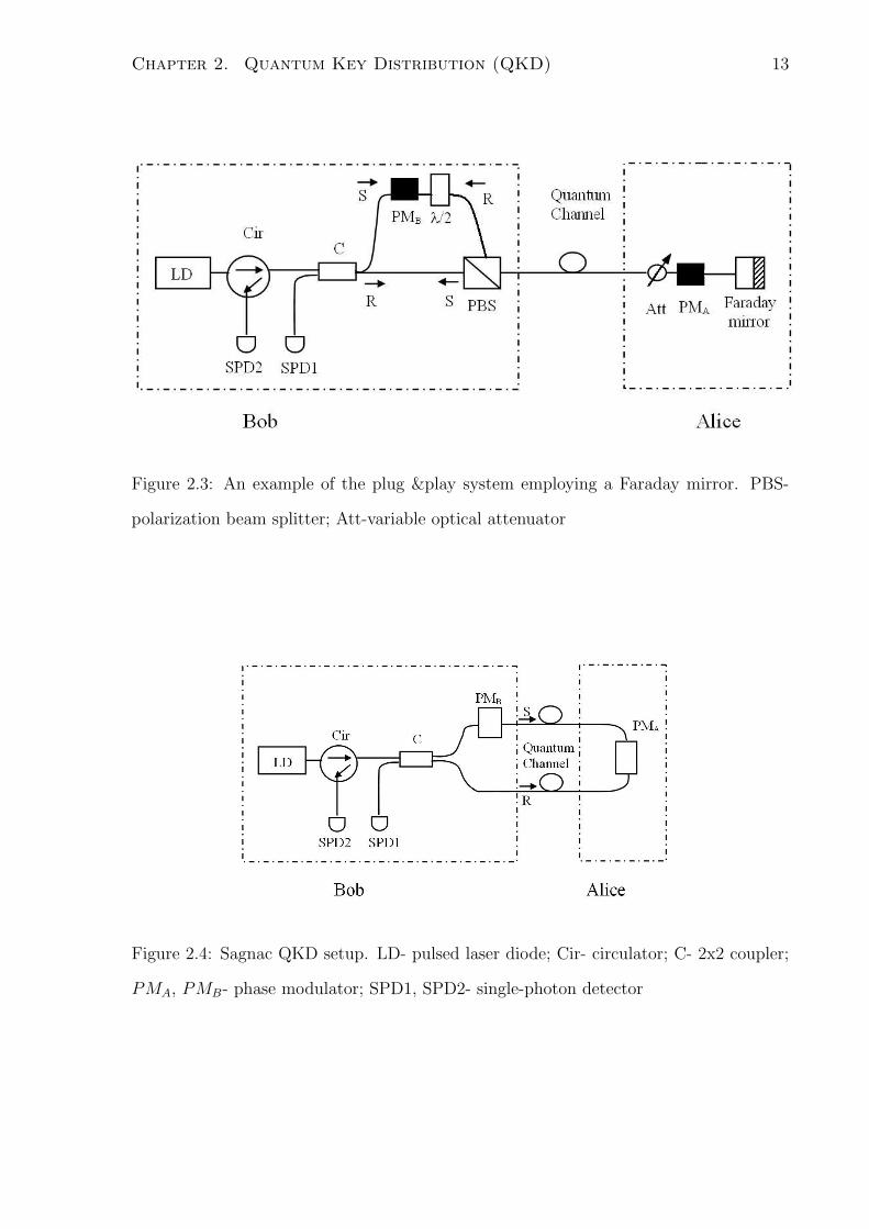
In the “plug & play” scheme (Figure 2.3), bright laser pulses are divided into two
by the coupler (C) on Bob’s side: one half is the reference pulse (R), the other is the
signal pulse (S). The signal pulse travels via the upper (longer) arm, and is reflected by
the polarization beam splitter (PBS) whereas the reference pulse travels via the lower
(shorter) arm, and is transmitted by the PBS. They both propagate through the quantum
channel towards Alice, and are reflected by the Faraday mirror (FM) at Alice’s end. Alice
then modulates the phase of the signal pulse to encode the relative phase information
using PMA but leave the reference pulse un-modulated. Both the signal and reference
pulses are sent back to Bob. When the pulses reach the PBS after their return trip, the
polarization states of the pulses are exactly orthogonal to what they were when they
left, due to the effect of the FM. At Bob’s AMZI, the signal pulse then travels via the
lower (shorter) arm while the reference pulse travels via the upper (longer) arm. In this
case, both the reference and signal pulses propagate through the same path and any slow
variations in the difference of the two paths in the AMZI are automatically canceled out.
Note the optical attenuator (Att) on Alice’s side is set so that when the pulses leave
Alice, each of them contains no more than a single photon. “Plug & play” scheme is now
the basis of commercial QKD systems [22].
Sagnac loop auto-compensating QKD structure is another kind of two-way QKD [20]
[21] [23]. As shown in Figure 2.4, the Sagnac loop offers phase stability as the two
interfering pulses (reference and signal) travel through the same fiber loop clockwise and
counterclockwise, respectively.
Although the two-way architecture can reduce the problem of phase drift, it degrades
the system performance, due to back scattering of outgoing strong pulses contaminating
the weak returning signals, resulting in an increased quantum bit error rate (QBER).
Chapter 2. Quantum Key Distribution (QKD) 13
Figure 2.3: An example of the plug &play system employing a Faraday mirror. PBS-
polarization beam splitter; Att-variable optical attenuator
Figure 2.4: Sagnac QKD setup. LD- pulsed laser diode; Cir- circulator; C- 2x2 coupler;
PMA, PMB- phase modulator; SPD1, SPD2- single-photon detector
Chapter 2. Quantum Key Distribution (QKD) 14
To minimize this affect, a two-way system needs to operate by sending bursts of pulses
spaced by long dead intervals [22]. This will reduce the duty cycle and the bit rate of
the system. The two-way system can also have other drawbacks such as the doubling of
the transmission loss, and its vulnerability towards the Trojan horse attack [24].
2.1.2 Continuous Variables QKD
Most of current QKD systems are based on single-photon QKD protocols. However,
experimental implementation of these protocols presents a few challenges. First of all,
strictly single-photon sources are not available. Secondly, single-photon detectors (SPDs)
are inefficient, especially in the telecommunication wavelength region. For instance,
at 1.5µm, typically, only 10 − 15% efficiency can be observed using InGaAs SPDs at
173K. Thirdly, single-photon signals are weak and offer poor signal-to-noise ratio (SNR),
especially in a lossy system. Therefore, single-photon key transmission typically has a
low efficiency and is limited by a short communication distance.
Due to the technical challenges and problems in the single photon QKD, recent interest
is developing in continuous-variable QKD [25] [26], where multi-photon bits are used.
Grosshans et al. demonstrated a new continuous-variable QKD protocol based on the
transmission of Gaussian-modulated coherent state (GMCS)[27]. Although a full security
proof of GMCS QKD against the most general type of attack is still pending, security
against individual attack has already been proved. The simplicity of using coherent light
pulses and the potentially high transmission efficiency offered by the GMCS QKD make
it highly attractive for practical implementation.
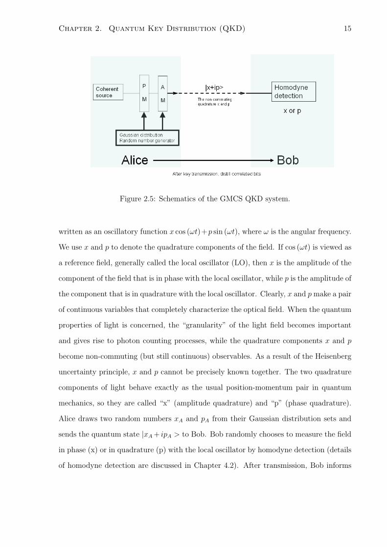
The basic scheme of GMCS QKD is illustrated in Figure 2.5. Alice generates two
independent sets of random numbers x and p with a Gaussian distribution (with the
mean at zero and a variance at VAN0, where N0 denotes the shot-noise variance). The
fact that both x and p are Gaussian random numbers allows an optimal information rate
through a Gaussian noisy channel [28]. In classical electromagnetism, a light field can be
Chapter 2. Quantum Key Distribution (QKD) 15
Figure 2.5: Schematics of the GMCS QKD system.
written as an oscillatory function x cos (ωt)+p sin (ωt), where ω is the angular frequency.
We use x and p to denote the quadrature components of the field. If cos (ωt) is viewed as
a reference field, generally called the local oscillator (LO), then x is the amplitude of the
component of the field that is in phase with the local oscillator, while p is the amplitude of
the component that is in quadrature with the local oscillator. Clearly, x and p make a pair
of continuous variables that completely characterize the optical field. When the quantum
properties of light is concerned, the “granularity” of the light field becomes important
and gives rise to photon counting processes, while the quadrature components x and p
become non-commuting (but still continuous) observables. As a result of the Heisenberg
uncertainty principle, x and p cannot be precisely known together. The two quadrature
components of light behave exactly as the usual position-momentum pair in quantum
mechanics, so they are called “x” (amplitude quadrature) and “p” (phase quadrature).
Alice draws two random numbers xA and pA from their Gaussian distribution sets and
sends the quantum state |xA + ipA > to Bob. Bob randomly chooses to measure the field
in phase (x) or in quadrature (p) with the local oscillator by homodyne detection (details
of homodyne detection are discussed in Chapter 4.2). After transmission, Bob informs
Chapter 2. Quantum Key Distribution (QKD) 16
Alice which quadrature he measured through an authenticated public channel. Alice
drops irrelevant data (the quadrature information which Bob did not choose to measure)
and share a set of correlated Gaussian variables -“key elements”- with Bob. Alice and
Bob then publicly compare a random sample of their key elements to evaluate the error
rate and transmission efficiency of the quantum channel. From the observed correlations,
Alice and Bob evaluate the amount of information they share (IAB = IBA) and the
maximum information Eve may have obtained about their values (IAE and IBE). It is
known that Alice and Bob can, in principle, distill from their key elements a common
secret key of size S > sup(IAB − IAE, IBA − IBE), in units of bits/symbol [29] [30].
This requires classical communication over an authenticated public channel, and may be
divided into two steps: reconciliation (i.e., correcting the errors while minimizing the
information revealed to Eve) and privacy amplification (i.e., making the key secret).
The security of GMCS QKD relies on the non-commuting quadrature components x
and p. The information of x and p cannot be jointly known according to the uncertainty
principle. For intercept-and-resend attack, if Eve only chooses one quadrature to measure
as in the BB84 intercept-and-resend attack, she will introduce 25% error rate if she
measured the wrong quadrature (the same situation as when Eve chooses the wrong basis
in BB84). However, for GMCS QKD, the transmitted quantum state is not embodied
in a single photon and it is possible to make simultaneous measurements of the two
quadratures. So a second strategy that Eve could follow would be to split the beam in
half, measure both quadratures (xA and pA)and send another coherent state with her
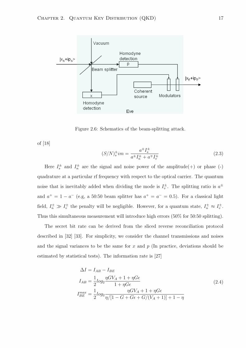
measured quadratures (xE and pE) to Bob (Figure 2.6).
If an ideal measurement of one quadrature amplitude produces a result with a SNR
of
(S/N)± =I±sI±n
(2.2)
then a simultaneous measurement of both quadratures cannot give a SNR result in excess
Chapter 2. Quantum Key Distribution (QKD) 17
Figure 2.6: Schematics of the beam-splitting attack.
of [18]
(S/N)±s im =a±I±s
a±I±n + a∓I±v(2.3)
Here I±s and I±n are the signal and noise power of the amplitude(+) or phase (-)
quadrature at a particular rf frequency with respect to the optical carrier. The quantum
noise that is inevitably added when dividing the mode is I±v . The splitting ratio is a±
and a+ = 1 − a− (e.g, a 50:50 beam splitter has a+ = a− = 0.5). For a classical light
field, I±n À I±v the penalty will be negligible. However, for a quantum state, I±n ≈ I±v .
Thus this simultaneous measurement will introduce high errors (50% for 50:50 splitting).
The secret bit rate can be derived from the sliced reverse reconciliation protocol
described in [32] [33]. For simplicity, we consider the channel transmissions and noises
and the signal variances to be the same for x and p (In practice, deviations should be
estimated by statistical tests). The information rate is [27]
∆I = IAB − IBE
IAB =1
2log2
ηGVA + 1 + ηGε
1 + ηGε
ImaxBE =
1
2log2
ηGVA + 1 + ηGε
η/[1−G + Gε + G/(VA + 1)] + 1− η
(2.4)
Chapter 2. Quantum Key Distribution (QKD) 18
0 0.1 0.2 0.3 0.4 0.5 0.6 0.7 0.8 0.9 10
0.5
1
1.5
2
2.5
3
Channel transmission (G)
Key
rat
e (b
its/s
ymbo
l)
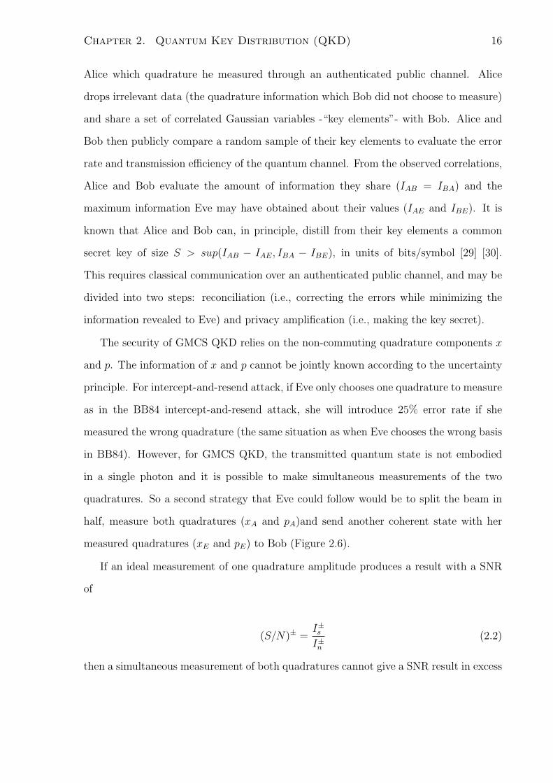
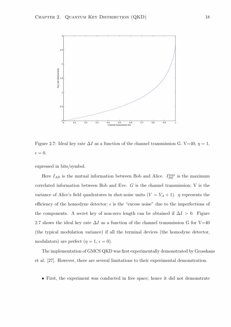
Figure 2.7: Ideal key rate ∆I as a function of the channel transmission G. V=40, η = 1,
ε = 0.
expressed in bits/symbol.
Here IAB is the mutual information between Bob and Alice. ImaxBE is the maximum
correlated information between Bob and Eve. G is the channel transmission; V is the
variance of Alice’s field quadratures in shot-noise units (V = VA + 1). η represents the
efficiency of the homodyne detector; ε is the “excess noise” due to the imperfections of
the components. A secret key of non-zero length can be obtained if ∆I > 0. Figure
2.7 shows the ideal key rate ∆I as a function of the channel transmission G for V=40
(the typical modulation variance) if all the terminal devices (the homodyne detector,
modulators) are perfect (η = 1, ε = 0).
The implementation of GMCS QKD was first experimentally demonstrated by Grosshans
et al. [27]. However, there are several limitations to their experimental demonstration.
• First, the experiment was conducted in free space; hence it did not demonstrate
Chapter 2. Quantum Key Distribution (QKD) 19
the feasibility of implementation in fiber communication networks.
• Second, the experiment was carried out with 780nm optical signals and therefore
did not take advantage of the low-cost, readily-available optical components in the
telecommunication wavelength.
• Third and more importantly, no random phase modulation was performed in their
experiment, rather, linear phase modulation was used. For such a deterministic
phase variation, the security of the protocol was not warranted, and thus strictly
speaking, no genuine secret key could be distributed.
• Fourth, Alice and Bob were not actually separated, rather, they were placed on the
same optical table.
• Finally, two different channels were used to transmit the signal and the local oscil-
lator, which means only one Mach-Zehnder interferometer was used for the QKD
system (similar to the one in Figure 2.1). As we discussed before, it is difficult to
keep the path difference between the signal arm and the local oscillator arm stable
with such a configuration in a real key transmission system.
Therefore, the experiment in [27] did not demonstrate the feasibility of a practical
communication system and requires future work.
2.2 State of the Art
In recent years, the widespread interest from industry and academia in QKD systems
has fueled the considerable progress in both theoretical and experimental QKD. One of
the most useful implementations is the Sagnac loop QKD, which is attractive because
of its phase stability, simple structure, as well as its possible extension to network QKD
systems. One of the most recent papers on Sagnac QKD experiment [23] before our work,

Chapter 2. Quantum Key Distribution (QKD) 20
achieved 87% interference visibility for a 5km fiber loop. As mentioned in Equation (2.1),
the QBER and the visibility have a relationship of QBER = (1−V )/2. There could not
be any key transmission with such a low visibility.
For the GMCS QKD system, the interest is increasing in the application of telecom-
munication fiber systems. Most recently, two papers have been published on fiber-based
GMCS QKD system [34] [35]. Lodewyck et al. [34] described a one-way GMCS QKD
system working at 1550 nm, and entirely made of standard fiber optics and telecom
components. However, the signal and the local oscillator are still transmitted in two
separate channels. As a result, their system is not stable and cannot support long dis-
tance transmission. Only a few meter fiber transmission distance is demonstrated even
with external perturbation isolation. Another paper presented by Legre et al. in [35],
demonstrated a 14km distance GMCS QKD system, based on a two-way system similar
to “plug & play”. As it is well known, the main disadvantage of “plug & play” configu-
ration is that it is susceptible to Trojan horse attack and thus cannot guarantee security.
Moreover, no quantum key exchange is demonstrated through their system. Rather, they
estimate the key rate according to measured system parameters. Therefore, more efforts
still have to be made to demonstrate a secure one-way fiber-based GMCS QKD system
in telecommunication wavelength and over a practical transmission distance.
2.3 Summary
An overview of quantum key distribution and the most well-known protocols have been
introduced in this chapter. We have also provided an overview of the experimental
implementations followed by their challenges and problems. Finally, the current status
of Sagnac and GMCS QKD experiments has been discussed. The goal of this thesis,
then, is to advance the state-of-the-art through the implementations of practical QKD
system with Sagnac loop and GMCS QKD in fiber-based system.
Chapter 3
Sagnac QKD with
Polarization-insensitive Phase
Modulators
In this chapter we first propose a novel polarization-insensitive phase modulation scheme
based on frequency modulation using a pair of acousto-optic modulators. We then employ
this technique to experimentally demonstrate a stable two-way quantum key distribution
(QKD) system with a Sagnac loop [19]. The highlight of this work is the polarization-
insensitive phase modulator which can significantly improve the performances of previous
Sagnac QKD systems. Finally, we show the experimental results and discuss potential
implementations. Our experiment is the first QKD demonstration based on the Sagnac
loop configuration over large distance.
3.1 Introduction
Due to the instability of the interferometer in QKD systems discussed in Chapter 2,
two-way auto-compensating QKD structures have been employed as practical solutions.
21

Chapter 3. Sagnac QKD with Polarization-insensitive Phase Modulators22
In the last few years, a two-way QKD system based on Sagnac interferometer has also
been proposed [20] [21] [23]. Compared with other two-way systems, Sagnac loop QKD
takes advantage of simple configuration and the ease of potential implementation in fu-
ture multi-users QKD networks. Unfortunately, due to the polarization sensitivity of the
commercial LiNbO3 waveguide phase modulator, complicated polarization controls are
required, which greatly degrades the performance of the previous Sagnac QKD demon-
strations [20] [23]. For example, six polarization controllers were employed in [20] and
four were used in [23]. It is not only difficult to control the system, but also difficult to
achieve high visibilities with so many polarization controllers. In [23], the interference
visibility for a 5km fiber loop was only 87% and no quantum key exchange has been
made experimentally due to such a low visibility. Although a quantum key distribution
is demonstrated in [20], the fiber transmission distance is only 200m.
Recently, we have presented a design of a high-speed polarization insensitive phase
modulator to be used in the Sagnac QKD system, which eliminates most of the polarizers
and is stable over several minutes without any recalibration [37]. Although this system
is designed for the BB84 protocol, with minimum modifications, it can also be used to
implement other protocols, such as decoy state QKD [12] [13] and continuous-variable
QKD [25] [27].
3.2 Polarization-insensitive Phase Modulators
The principle of the polarization-insensitive phase modulation scheme is shown in Fig-
ure 3.1, constructed by placing a frequency shift element in a Sagnac interferometer
asymmetrically.
In Figure 3.1(a), the input laser pulse is split by the fiber coupler into S1 and S2,
which go through the fiber loop clockwise and counterclockwise, respectively. Note that a
first-order acousto-optic modulator (AOM +) is placed in the fiber loop asymmetrically,
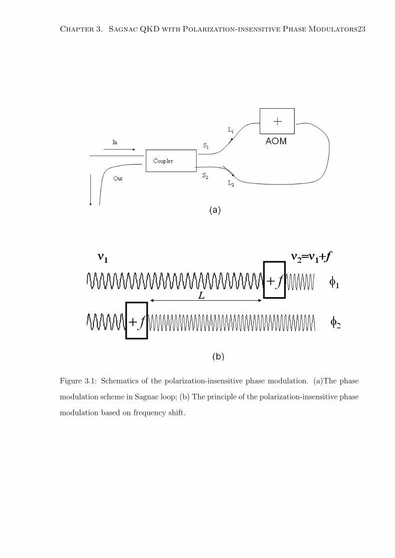
Chapter 3. Sagnac QKD with Polarization-insensitive Phase Modulators23
Figure 3.1: Schematics of the polarization-insensitive phase modulation. (a)The phase
modulation scheme in Sagnac loop; (b) The principle of the polarization-insensitive phase
modulation based on frequency shift.

Chapter 3. Sagnac QKD with Polarization-insensitive Phase Modulators24
with fiber lengths on each side being L1 and L2 . Due to the Doppler Effect, for the
first order diffraction light, the AOM introduces a frequency shift equal to its driving
frequency f . If the original optical frequency of S1 and S2 is ν1, then the resulting
frequency is ν2 = ν1 + f . As illustrated in Figure 3.1(b), because the AOM is placed
asymmetrically, S1 and S2 have different frequencies when S1 has passed through the
AOM and S2 has not. An additional phase difference between S1 and S2 is introduced
after completing the loop:
∆φ = φ2 − φ1 = 2πn(L2 − L1)(ν2 − ν1)/c = 2πnLf/c (3.1)
Here n is refractive index of optical fiber and c is the speed of light in vacuum.
By modulating the AOM’s driving frequency f , the relative phase between S1 and S2
can be modulated. This is the basic operation principle of our AOM-based phase mod-
ulator. Since the relative phase is introduced by frequency shift, this phase modulation
scheme is polarization-insensitive.
We remark that in the scheme, depicted in Figure 3.1, the resulting S1 and S2 will have
a frequency shift f . If we apply the scheme to a real QKD system directly, the encoded
phase information can be calculated from Equation (3.1) if Eve is able to measure the
shifted frequency f . This may leak additional information to Eve and invalidate the
unconditional security proof for standard BB84 protocol.
A simple and straightforward solution to reduce this f frequency shift can be achieved
by employing two AOMs, one up-shifting (+) and one down-shifting (-), separated by a
fiber length L, as shown in Figure 3.2.
Since the two AOMs (one in +1 diffraction order, the other in -1 diffraction order) are
driven by the same driver, they will shift the frequency of light by the same amount but
with different signs. After traveling through the two AOMs, the net optical frequency
shift will be zero. As the down-shifting AOM will shift the phase of the diffracted light
with an opposite sign, during the L length between the two AOMs, S1 has a frequency

Chapter 3. Sagnac QKD with Polarization-insensitive Phase Modulators25
Figure 3.2: Polarization-insensitive phase modulator with a pair of AOMs, +: up-shifting
AOM, -: down-shifting AOM, L: fiber length L between two AOMs, D: AOM driver
of ν2 = ν1 + f while S2 has a frequency of ν3 = ν1 − f . The additional phase difference
between S1 and S2 introduced by the two AOMs is
∆φ = φS2 − φS1 = 2πnL(ν2 − ν3)/c = 4πnLf/c (3.2)
Again, phase modulation can be achieved by modulating f .
Compared with the commercial LiNbO3 waveguide-based phase modulator, this novel
phase modulator has the following advantages.
• Polarization insensitive. Polarization-insensitive phase modulator can greatly re-
duce the difficulty of polarization adjustment in the conventional Sagnac QKD
system.
• High phase resolution. The phase modulation can be controlled precisely by the
acoustic frequency f , in order of 10−6, which is much better than LiNbO3 waveguide-
based phase modulator (about 10−2).
• Adjustable frequency-to-phase ratio. Since the fiber length between two AOMs is
tunable, according to Equation (3.2), the frequency f to phase ∆φ ratio is ad-
justable.
Chapter 3. Sagnac QKD with Polarization-insensitive Phase Modulators26
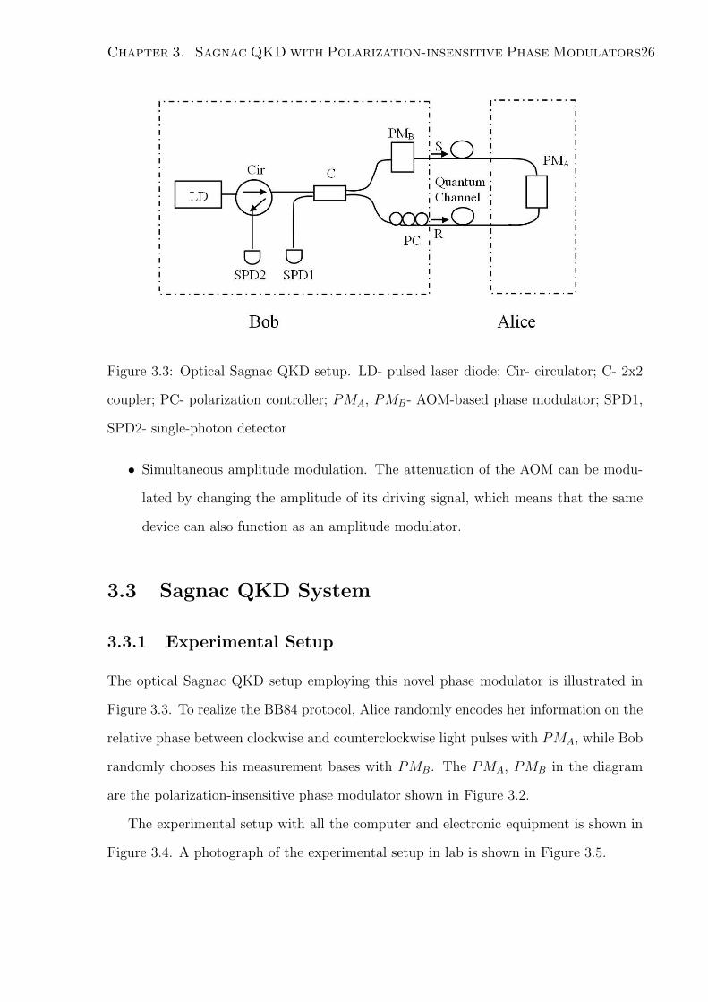
Figure 3.3: Optical Sagnac QKD setup. LD- pulsed laser diode; Cir- circulator; C- 2x2
coupler; PC- polarization controller; PMA, PMB- AOM-based phase modulator; SPD1,
SPD2- single-photon detector
• Simultaneous amplitude modulation. The attenuation of the AOM can be modu-
lated by changing the amplitude of its driving signal, which means that the same
device can also function as an amplitude modulator.
3.3 Sagnac QKD System
3.3.1 Experimental Setup
The optical Sagnac QKD setup employing this novel phase modulator is illustrated in
Figure 3.3. To realize the BB84 protocol, Alice randomly encodes her information on the
relative phase between clockwise and counterclockwise light pulses with PMA, while Bob
randomly chooses his measurement bases with PMB. The PMA, PMB in the diagram
are the polarization-insensitive phase modulator shown in Figure 3.2.
The experimental setup with all the computer and electronic equipment is shown in
Figure 3.4. A photograph of the experimental setup in lab is shown in Figure 3.5.

Chapter 3. Sagnac QKD with Polarization-insensitive Phase Modulators27
Figure 3.4: Sagnac QKD experimental setup. Laser: 1550nm cw laser; AM: ampli-
tude modulator; VOA: variable optical attenuator; Cir: circulator; C: 2x2 coupler; PC:
polarization controller; MFG: main function generator; PG: pulse generator; DG: De-
lay generator; SPD1, SPD2: single-photon detector; AOM+: up-shifting AOM; AOM-:
down-shifting AOM; PMA, PMB: Alice and Bob’s phase modulators (each consists of
one AOM+ and one AOM-); DRA, DRB: AOM drivers for PMA and PMB

Chapter 3. Sagnac QKD with Polarization-insensitive Phase Modulators28
Figure 3.5: The full Sagnac QKD system in laboratory
The amplitude modulator (AM) is used to produce 500ps laser pulses, controlled
by a pulse generator (PG). The main function generator (MFG) triggers the PG, as
well as the delay generator (DG). The DG provides a clock signal for the computer to
read data from the detectors and update AOM driving frequencies. Pulses are split by
a 50/50 fiber coupler (C) and then travel through a long fiber loop (≈ 40km) in the
clockwise and counterclockwise directions, respectively. Each AOM pairs are controlled
by an AOM driver (DRA and DRB), which essentially is a simple function generator.
The AOM drivers allow the amplitude and frequency to be modulated by voltage levels.
For BB84 QKD implementation, modulator PMA is used to randomly encode one of the
four states {0, π/2, π, 3π/2} and a variable optical attenuator (VOA) is employed to
reduce the average photon number to 0.8 photon/pulse, measured at the output of Alice.
Bob then randomly chooses his measurement bases {0, π/2} by modulating his phase
modulator PMB. A polarization controller (PC) inside the Sagnac loop is employed to
compensate for the birefringence of the fiber loop. The clockwise and counterclockwise
pulses interfere at C upon completing the loop and are detected by two InGaAs single
Chapter 3. Sagnac QKD with Polarization-insensitive Phase Modulators29
photon detectors (SPD, Id Quantique, id200). The SPDs work in the gated mode to
reduce the dark counts. Working in gated mode means that the SPDs are only open to
detect photons for a small time window (<5ns). The gates for SPDs are controlled by
trigger signals, which also come from the DG. Computer controlled data acquisition card
(DAQ card) is used to control encoding and decoding.
Since the AOM-based phase modulators are polarization insensitive, the system is
implemented entirely with standard single mode fibers. Our Sagnac QKD system greatly
reduces the number of polarization controllers and avoids the need for complex polariza-
tion adjustments, making the entire system stable, low loss and easy to implement.
3.3.2 Synchronization
In our experiment, we need to synchronize the triggers for the SPDs, the triggers for the
AOMs’ drivers, and the trigger for the DAQ card to starting reading from the SPDs.
The delay generator (DG) is used for these timing control. DG has four outputs with
independently controlled time delays, two are used for SPDs’ synchronization while the
other two are for Alice and Bob’s modulations respectively.
In Figure 3.4, the light pulses travel about 20km of fiber to get to Alice, and 20km
more to get back to Bob. The total time it takes for a light pulse to go around the fiber
loop is about 198.2µs. The Delay A (to trigger SPD1) and Delay B (to trigger SPD2)
from DG are set to around 198.2µs. Then, we find the optimal delay time by maximizing
the efficiency of each SPD. The final result is that Delay A is set to be 198.266µs and
Delay B is 198.2775µs. Note Delay B is 11.5ns longer than Delay A because signals that
go to SPD2 have to travel a few meters more than those go to SPD1.
When the SPD clicks, it sends an electrical signal about 200ns wide to the computer.
Since the optical pulse does not happen every time (for example, in case of an empty
pulse), in order to detect each non-empty pulse, the computer has to check every time
there may be a pulse. Hence the computer’s clock signal (Delay C) triggers at around
Chapter 3. Sagnac QKD with Polarization-insensitive Phase Modulators30
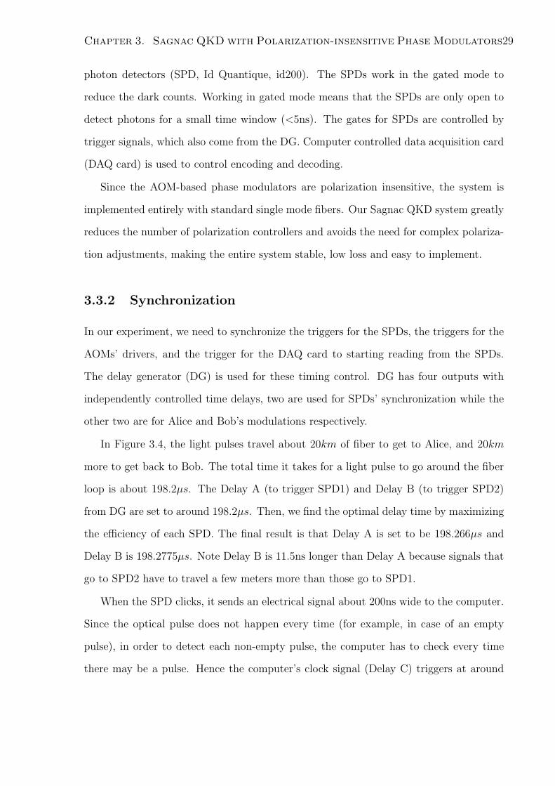
Figure 3.6: Bob’s synchronization in the Sagnac QKD system
the same time as the triggers for the SPDs to detect each electrical pulse sent by the
SPDs.
The delay generator also provides a clock signal for the computer to output analog
voltages to Alice and Bob’s AOM drivers. For Alice, the computer outputs an analog
voltage to the AOM driver which in turns sets the frequency of her AOM’s. Hence, Alice
can encode one of the 4 phases {0, π/2, π, 3π/2} by setting the appropriate voltage level.
For Bob’s AOM, the situation is more complicated because Bob only wants to mod-
ulate the arriving light pulses but not the ones leaving. In this case, the repetition rate
should be carefully chosen that the arriving and leaving pulses are separated as much as
possible. Bob should only output a short pulse to modulate the arriving pulses, as shown
in Figure 3.6.
3.4 Experimental Results
By scanning the output voltages sent to DRA and DRB respectively, we are able to
change the relative phase between S1 and S2 by using PMA or PMB. In this case, the
Chapter 3. Sagnac QKD with Polarization-insensitive Phase Modulators31
interference visibility can be measured from the counts of the two SPDs. When the
average output photon number from Alice’s side is set to 0.8 photon/pulse, we achieved
high visibility (96%) for a 40km fiber loop. This is considerably higher than previously
reported values (87%) and the distance in our set up is also considerably longer (40km
vs. 5km).
In the QKD experiment, two random number files are preloaded to the Alice’s and
Bob’s buffers on the DAQ card. Alice’s contains a series of discrete random numbers
corresponding to the four phase states {0, π/2, π, 3π/2} in the BB84 protocol. Bob’s
contains the same size of discrete random numbers corresponding to {0, π/2} basis choice.
When the DAQ card detects a trigger signal, which comes from a delay generator, it starts
to read out a number from Alice’s buffer and send it to DRA for phase encoding. The
DAQ card subsequently reads out a number from Bob’s buffer and sends it to DRB to
choose the measurement basis. The DAQ card also samples the outputs from the two
SPDs into its digital input buffer.
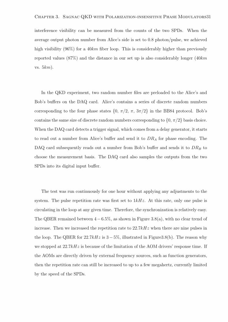
The test was run continuously for one hour without applying any adjustments to the
system. The pulse repetition rate was first set to 1kHz. At this rate, only one pulse is
circulating in the loop at any given time. Therefore, the synchronization is relatively easy.
The QBER remained between 4−6.5%, as shown in Figure 3.8(a), with no clear trend of
increase. Then we increased the repetition rate to 22.7kHz when there are nine pulses in
the loop. The QBER for 22.7kHz is 3− 5%, illustrated in Figure3.8(b). The reason why
we stopped at 22.7kHz is because of the limitation of the AOM drivers’ response time. If
the AOMs are directly driven by external frequency sources, such as function generators,
then the repetition rate can still be increased to up to a few megahertz, currently limited
by the speed of the SPDs.

Chapter 3. Sagnac QKD with Polarization-insensitive Phase Modulators32
Figure 3.7: The interference visibilities of the Sagnac QKD system. (a) The interfer-
ence visibility achieved by modulating PMA; (b) The interference visibility achieved by
modulating PMB.
Chapter 3. Sagnac QKD with Polarization-insensitive Phase Modulators33
Figure 3.8: Experimental QBER for the Sagnac QKD system. The QBER is plot against
time. (a) QBER of 1kHz repetition rate without recalibration; (b) QBER of 22.7kHz
repetition rate without recalibration.
Chapter 3. Sagnac QKD with Polarization-insensitive Phase Modulators34
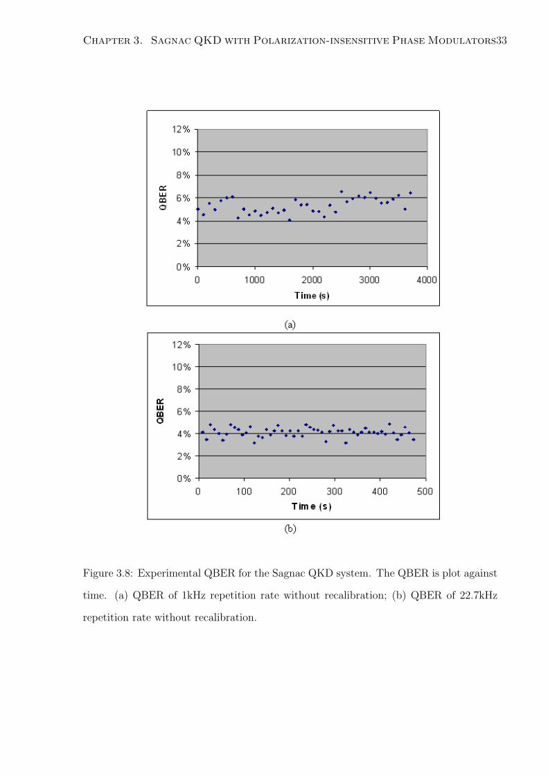
Figure 3.9: The optical-ring QKD network based on the Sagnac interferometer.
3.5 Summary
Recently, interest is increasing in Sagnac QKD. Compared with the other topologies,
such as the passive-star network, the wavelength-routed network, and the wavelength-
addressed bus network, the optical-ring network based on the Sagnac interferometer has
the best performance.
• Firstly, it has the simplest design, requiring each user to have only one phase
modulator (Figure 3.9). This is a major benefit since the capital invested in the
individual user is low. Note for the previous Sagnac QKD system [23], since the
phase modulator is polarization sensitive, it is very difficult and not realistic for
each user to adjust so many polarization controllers every time before transmission.
• Secondly, the ring network is also more stable against polarization and phase fluc-
tuations than the other topologies since both the reference and signal pulses travel
through the same ring path [38].

Chapter 3. Sagnac QKD with Polarization-insensitive Phase Modulators35
Our setup Ref [23]
Visibility 96% 87%
Fiber loop length 40km 5km
Raw key repetition rate 1kHz/22.7kHz no key exchange
Experiment Duration 60min / 10min no key exchange
QBER 4− 6.5% / 3− 5% no key exchange
Table 3.1: Experimental Sagnac QKD results compared with the most recent demonstra-
tion.
• Thirdly, it is proven in [36] that due to its efficient design, the ring topology has
the lowest loss overhead among the networks that were compared and as a result
has the lowest QBER and highest sifted key rate for networks with less than 60
users.
The great configuration simplification and performance improvement of our Sagnac loop
QKD system make it easy to obtain a stable, fast-speed, and long distance Sagnac QKD
ring network towards a practical quantum cryptography system.
In our Sagnac QKD system, though we only implemented the BB84 protocol, with a
few modifications, we can easily implement other protocols using this system, such as the
decoy state QKD [12] [13] and the continuous-variable QKD [25] [27]. This is because the
transmittance of an AOM can also be modulated by the amplitude of its driving signal,
which means an AOM itself can both function as an amplitude modulator and a phase
modulator.
In conclusion, we have demonstrated an experimental Sagnac QKD system with
AOM-based polarization-insensitive phase modulators. Our system offers a much simpler
configuration, more stable performance, and longer transmission distance than previous
demonstrations. Compared with the most recent reported Sagnac QKD system in [23],
which gives a 87% visibility with a 5km fiber loop, our system has a high visibility of 96%

Chapter 3. Sagnac QKD with Polarization-insensitive Phase Modulators36
with a 40km fiber loop. We make a quantum key exchange on our Sagnac system, and
are able to achieve a QBER between 4−6.5% for over one hour without any recalibration.
Chapter 4
Gaussian-modulated Coherent
States (GMCS) QKD System Design
Recently, it has been proposed theoretically that continuous-variable quantum key dis-
tribution (QKD) protocols are able to obtain a higher quantum bit rate than the usual
photon-counting techniques. In this chapter, a GMCS system implemented in standard
fiber and entirely made of telecom components is investigated. The system configuration,
design of each specific component, and solutions to different challenges are discussed and
compared. Finally, the entire experimental system setup is described.
4.1 System Design
The Gaussian-modulated coherent states QKD protocol runs as discussed in Section 2.
According to the protocol procedure, our initial system design was shown in Figure 4.1.
Our objective is to implement GMCS QKD protocol by transmitting Gaussian-modulated
coherent states over telecom fiber. In Figure 4.1, an amplitude and phase modulator
(AM&PM) on Alice’s side is used to encode the coherent state while a phase modulator
(PM) on Bob’s side is used to choose quadratures. A Piezoelectric Transducer (PZT) is
used to compensate for the phase drift. There are some disadvantages of this proposed
37

Chapter 4. Gaussian-modulated Coherent States (GMCS) QKD System Design38
Figure 4.1: Initial GMCS configuration. 1-1550nm CW laser; 2, 19-polarization con-
troller; 3- amplitude modulator; 4, 9, 11, 14, 16, 17, 20, 23, 25, 29, 31, 35, 36- fiber
collimator; 5, 8, 13, 22, 26, 28, 32, 33- λ/2 wave plate; 6, 12, 21, 27 - polarization beam
splitter; 7- PZT (Piezoelectric Transducer) based optical length adjust system; 10, 30-
polarization maintaining fiber; 15- phase and amplitude modulator; 18- single mode fiber;
24- phase modulator; 34- beam splitter; 37- homodyne detector
Chapter 4. Gaussian-modulated Coherent States (GMCS) QKD System Design39
configuration.
• Large component counts. The configuration shown in 4.1 is complicated. 14 colli-
mators, 8 half wave plates and 5 polarization beam splitters are employed in this
setup.
• Alignment complexity. It is difficult to align the light beam to travel through all
components in the proper direction. It also requires adjustment for collimators
for high coupling efficiency and rotation for half wave plates for right polarization
states.
• Instability. All the components have to be carefully aligned. A tiny vibration and
misalignment for each component would contribute to the instability of the entire
system. This setup is susceptible to external perturbations.
• High insertion loss. Due to large number of components, the insertion loss of the
entire system is relatively high. Especially for the free space to fiber coupling, each
of them has a low efficiency of ∼ 50%.
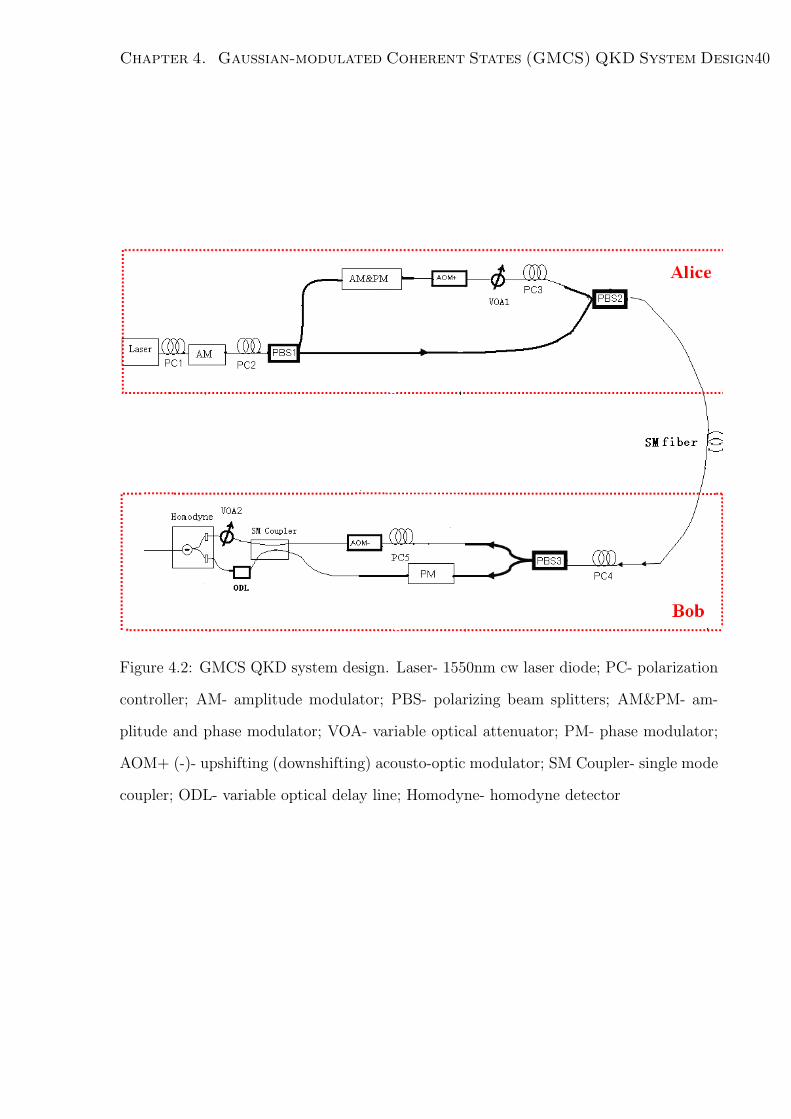
In order to solve these problems, a greatly simplified all-fiber-based configuration is
proposed, as shown in Figure 4.2. The elimination of the collimators and half wave plates
ensures better stability and low losses, as well as the ease of calibration and adjustment.
Details of each specific part will be discussed in the following sections.
4.2 Homodyne Detection Design
The detection technique used for GMCS QKD protocol is the balanced homodyne de-
tection. Compared with photon-counting technique in single-photon protocols, the ho-
modyne detectors have a higher efficiencies (typically 60 ∼ 80%) than the single photon
detectors (typically 10 ∼ 20%). The principle of standard homodyne detection is shown
in Figure 4.3. This detection is used to measure the x and p quadratures of weak signals.
Chapter 4. Gaussian-modulated Coherent States (GMCS) QKD System Design40
Figure 4.2: GMCS QKD system design. Laser- 1550nm cw laser diode; PC- polarization
controller; AM- amplitude modulator; PBS- polarizing beam splitters; AM&PM- am-
plitude and phase modulator; VOA- variable optical attenuator; PM- phase modulator;
AOM+ (-)- upshifting (downshifting) acousto-optic modulator; SM Coupler- single mode
coupler; ODL- variable optical delay line; Homodyne- homodyne detector

Chapter 4. Gaussian-modulated Coherent States (GMCS) QKD System Design41
Figure 4.3: Schematics of the balanced homodyne detection. PM- phase modulator; “-”-
differential amplifier; BS-beam splitter; θ- phase modulation for quadrature choice (0 or
π/2); Er, Es- electrical field of the local oscillator and the signal; Ir, It- reflected and
transmitted interference intensity; I- differential output (Ir − It) from the detector.
As we can see from the figure, the two light beams (the signal Es cos (ωt + φ) and the
local oscillator Er cos (ωt)) interfere on a 50/50 splitter. The output I from the homo-
dyne detector is the difference between the reflected (from signal point of view) output
Ir and the transmitted output It. Note here the beam splitter should be exactly 50/50
splitting in order to cancel out the DC components of Ir and It. This is where the word
“balanced” comes from. I is then proportional to either the amplitude quadrature (x) or
the phase quadrature (p), depending on whether a 0 or π/2 phase modulation is applied
on the signal arm. Because I is also proportional to the intensity of the local oscillator,
the local oscillator is much stronger (typically 6 orders of magnitude stronger) than the
signal for easy detection of the weak signal.
The homodyne detector is the most critical part in the GMCS QKD system and has
to be homemade in our experiment because of its stringent requirements. For example,
in order to achieve a positive secret key rate, the homodyne detector has to be shot-noise
Chapter 4. Gaussian-modulated Coherent States (GMCS) QKD System Design42
limited, which means the electrical noise should be much smaller than the shot noise.
The reason for this can be explained as follows. From Chapter 2, the secret key rate of
GMCS QKD protocol is
∆I = IAB − IBE
IAB =1
2log2
ηGVA + 1 + ηGε
1 + ηGε
ImaxBE =
1
2log2
ηGVA + 1 + ηGε
η/[1−G + Gε + G/(VA + 1)] + 1− η
(4.1)
expressed in bits/symbol.
Here IAB is the mutual information between Bob and Alice. ImaxBE is the maximum
correlated information between Bob and Eve. G is the channel transmission; V is the
variance of Alice’s field quadratures in shot-noise units (V = VA + 1). η represents the
efficiency of the homodyne detector; ε is the “excess noise” due to the imperfections of
the components.
According to the Equation (4.1), the smaller ε becomes, the higher the key rate could
be derived with a certain G. If the key is transmitted over a long distance, that is G ¿ 1,
from Equation (4.1), the secret key can only be obtained if ε < (V −1)/(2V ) ≈ 1/2, in the
unit of shot-noise variance (N0). This means that the amount of excess noise ε should not
be larger than half of the shot noise. The electrical noise of the homodyne detector (Ne)
is one contribution to the excess noise, the smaller Ne is, the smaller ε is. We must have
Ne < ε < 1/2N0 to achieve a positive secret key rate. Typically, the electrical noise of
the detector is 15-20dB below the shot noise. In quantum optics, shot noise is caused by
the fluctuations of detected photons, again therefore a consequence of discretization (of
the energy in the electromagnetic field). In the case of a coherent light source, the shot
noise(standard deviation of the noise) scales as the square-root of the average intensity:
∆I =√
I [41]. For an intensity of 108photons/pulse local oscillator (the typical value for
GMCS QKD), its shot noise intensity is on the order of 104photons/pulse. Therefore,
the electrical noise level should be on the order of 102 photons/pulse. No commercial
Chapter 4. Gaussian-modulated Coherent States (GMCS) QKD System Design43
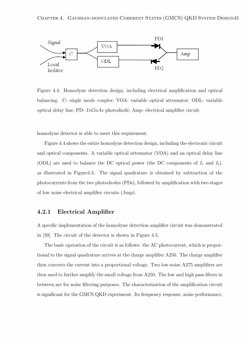
Figure 4.4: Homodyne detection design, including electrical amplification and optical
balancing. C- single mode coupler; VOA- variable optical attenuator; ODL- variable
optical delay line; PD- InGaAs photodiode; Amp- electrical amplifier circuit.
homodyne detector is able to meet this requirement.
Figure 4.4 shows the entire homodyne detection design, including the electronic circuit
and optical components. A variable optical attenuator (VOA) and an optical delay line
(ODL) are used to balance the DC optical power (the DC components of Ir and It),
as illustrated in Figure4.3. The signal quadrature is obtained by subtraction of the
photocurrents from the two photodiodes (PDs), followed by amplification with two stages
of low noise electrical amplifier circuits (Amp).
4.2.1 Electrical Amplifier
A specific implementation of the homodyne detection amplifier circuit was demonstrated
in [39]. The circuit of the detector is shown in Figure 4.5.
The basic operation of the circuit is as follows: the AC photocurrent, which is propor-
tional to the signal quadrature arrives at the charge amplifier A250. The charge amplifier
then converts the current into a proportional voltage. Two low-noise A275 amplifiers are
then used to further amplify the small voltage from A250. The low and high pass filters in
between are for noise filtering purposes. The characterization of the amplification circuit
is significant for the GMCS QKD experiment. Its frequency response, noise performance,
Chapter 4. Gaussian-modulated Coherent States (GMCS) QKD System Design44
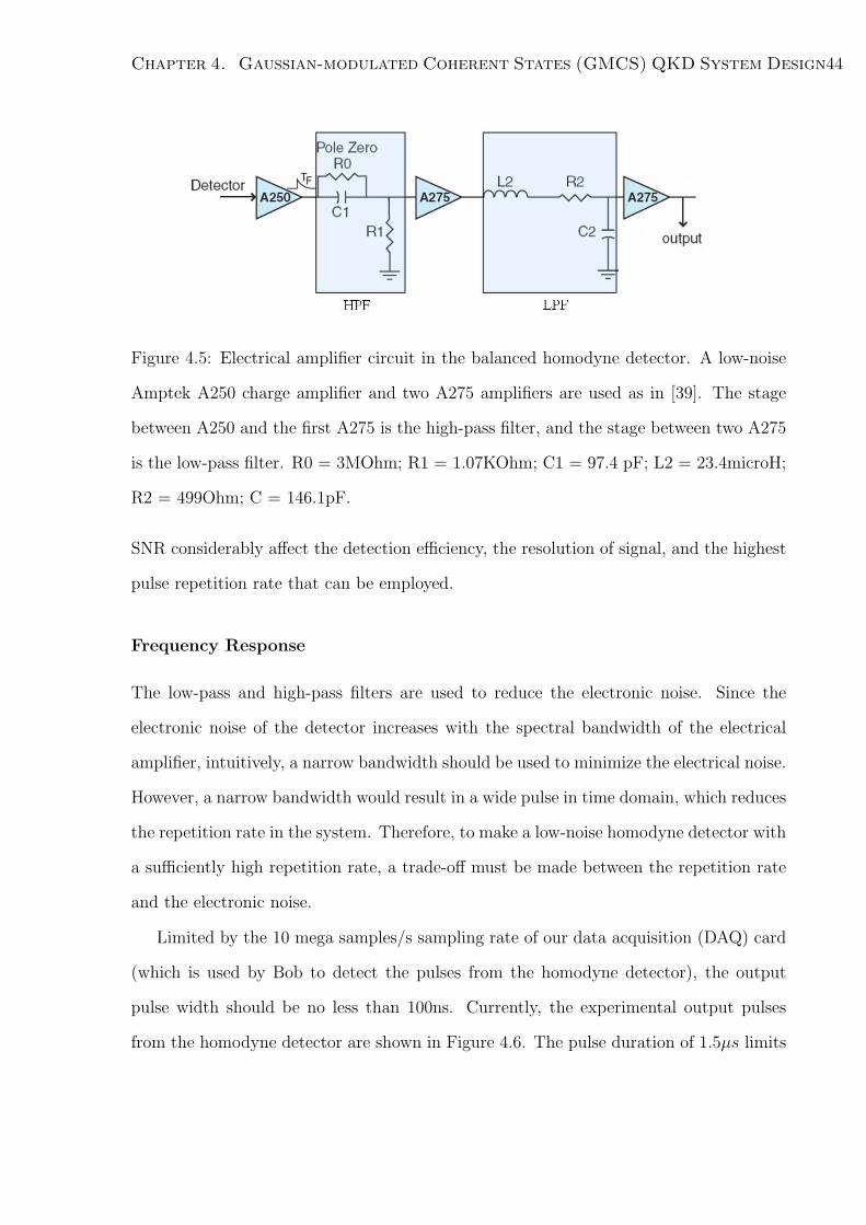
Figure 4.5: Electrical amplifier circuit in the balanced homodyne detector. A low-noise
Amptek A250 charge amplifier and two A275 amplifiers are used as in [39]. The stage
between A250 and the first A275 is the high-pass filter, and the stage between two A275
is the low-pass filter. R0 = 3MOhm; R1 = 1.07KOhm; C1 = 97.4 pF; L2 = 23.4microH;
R2 = 499Ohm; C = 146.1pF.
SNR considerably affect the detection efficiency, the resolution of signal, and the highest
pulse repetition rate that can be employed.
Frequency Response
The low-pass and high-pass filters are used to reduce the electronic noise. Since the
electronic noise of the detector increases with the spectral bandwidth of the electrical
amplifier, intuitively, a narrow bandwidth should be used to minimize the electrical noise.
However, a narrow bandwidth would result in a wide pulse in time domain, which reduces
the repetition rate in the system. Therefore, to make a low-noise homodyne detector with
a sufficiently high repetition rate, a trade-off must be made between the repetition rate
and the electronic noise.
Limited by the 10 mega samples/s sampling rate of our data acquisition (DAQ) card
(which is used by Bob to detect the pulses from the homodyne detector), the output
pulse width should be no less than 100ns. Currently, the experimental output pulses
from the homodyne detector are shown in Figure 4.6. The pulse duration of 1.5µs limits

Chapter 4. Gaussian-modulated Coherent States (GMCS) QKD System Design45
Figure 4.6: Typical output signal from the balanced homodyne detector. The amplitude
(200mV/div) of the pulse is plot against time (2µs/div). The input optical pulses are
100ns and the output pulses have a response pulsewidth of 1.5µs.
our current repetition rate to a few hundreds of kHz. In this case, the DAQ card can
record about ten samples for each pulse to rebuild the pulse shape. The present values
of the components for low-pass and high-pass filters are listed in Figure 4.5 and the
corresponding frequency response of the electrical amplifier circuit is shown in Figure
4.7.
The output pulse duration can be changed by changing the low-pass and high-pass
filters. For the homodyne detector itself, we can actually get a output pulse narrower than
1.5µs. For example, by changing the values of R1 and L2, we are able to obtain a 250ns
output pulse, shown in Figure 4.8. If we can replace our slow DAQ card (10Ms/s) with
a faster one, or use faster electronics such as a field programmable gate array (FPGA),
the repetition rate may be increased to several MHz.
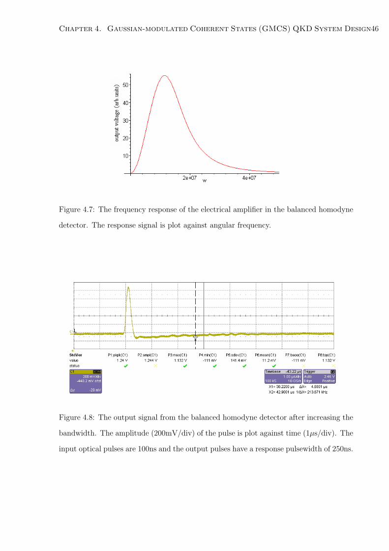
Chapter 4. Gaussian-modulated Coherent States (GMCS) QKD System Design46
Figure 4.7: The frequency response of the electrical amplifier in the balanced homodyne
detector. The response signal is plot against angular frequency.
Figure 4.8: The output signal from the balanced homodyne detector after increasing the
bandwidth. The amplitude (200mV/div) of the pulse is plot against time (1µs/div). The
input optical pulses are 100ns and the output pulses have a response pulsewidth of 250ns.

Chapter 4. Gaussian-modulated Coherent States (GMCS) QKD System Design47
Electronic Noise
The electronic noise of the amplifier circuit is measured, as shown in Figure 4.9. Origi-
nally, our measured electronic noise 4.9 (a) was relatively high compared with the previous
demonstration [39]. In order to avoid external perturbations, the entire circuit is enclosed
in a metal box. Moreover, batteries are used for the photodiode to offer a more stable
voltage supply. The electronic noise of the balanced homodyne detector after all these
modifications, is shown in Figure 4.9(b). The standard deviation (sdev) of the present
electronic noise is 1.2mV. The 8-bit oscilloscope itself, however, has a quantization er-
ror with a sdev of 0.444mV, as shown in 4.9(c). All in all, the sdev of the electronic
noise of the amplifier itself is√
1.22 − 0.442 mV=1.1mV. Less electronic noise can also
be achieved by narrowing down the spectral bandwidth of the electrical amplifier, as
discussed earlier.
4.2.2 Optical Balancing
To achieve balanced homodyne detection, the local oscillator into photodiodes PD1 and
PD2 (in Figure 4.4) should be well balanced. However, due to the imperfection of the
50/50 coupler as well as the different arrival times of the pulses, and the different efficien-
cies of the photodiodes, a variable optical attenuator (VOA) and a variable optical delay
line (ODL) are required to equalize the DC optical powers impinging upon the photodi-
odes. Although the implementation of VOA and ODL in Figure 4.4 help to balance the
DC signal, their insertion loss will decrease the efficiency of homodyne detection. The
present efficiency of the homodyne detector is about 56%, which includes the efficiency
of the photodiodes, the fiber connection losses and the insertion loss of the VOA. To
enhance the information rate, losses within the homodyne detector can be reduced by
replacing the attenuator with fiber bending. Moreover, all the connections can be spliced
to yield less loss.

Chapter 4. Gaussian-modulated Coherent States (GMCS) QKD System Design48
Figure 4.9: Electronic noise of the electrical amplifier in the balanced homodyne detector.
(a) The electronic noise before modification. The amplitude (5mV/div) of the noise is
plot against time (20µs/div); (b)Current electronic noise, including the noises of both
the amplifier and the oscilloscope. The amplitude (2mV/div) of the noise is plot against
time (20µs/div); (c) The noise of the oscilloscope, due to its quantization error and other
imperfections. The amplitude (2mV/div) of the noise is plot against time (20µs/div).
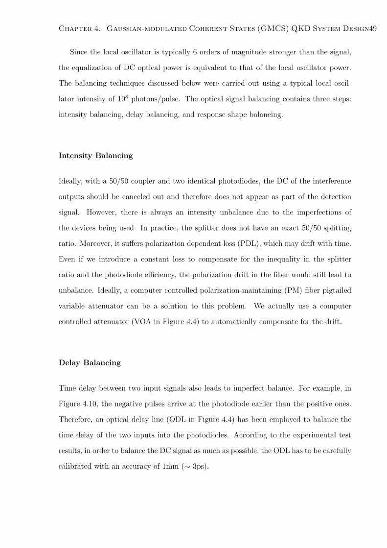
Chapter 4. Gaussian-modulated Coherent States (GMCS) QKD System Design49
Since the local oscillator is typically 6 orders of magnitude stronger than the signal,
the equalization of DC optical power is equivalent to that of the local oscillator power.
The balancing techniques discussed below were carried out using a typical local oscil-
lator intensity of 108 photons/pulse. The optical signal balancing contains three steps:
intensity balancing, delay balancing, and response shape balancing.
Intensity Balancing
Ideally, with a 50/50 coupler and two identical photodiodes, the DC of the interference
outputs should be canceled out and therefore does not appear as part of the detection
signal. However, there is always an intensity unbalance due to the imperfections of
the devices being used. In practice, the splitter does not have an exact 50/50 splitting
ratio. Moreover, it suffers polarization dependent loss (PDL), which may drift with time.
Even if we introduce a constant loss to compensate for the inequality in the splitter
ratio and the photodiode efficiency, the polarization drift in the fiber would still lead to
unbalance. Ideally, a computer controlled polarization-maintaining (PM) fiber pigtailed
variable attenuator can be a solution to this problem. We actually use a computer
controlled attenuator (VOA in Figure 4.4) to automatically compensate for the drift.
Delay Balancing
Time delay between two input signals also leads to imperfect balance. For example, in
Figure 4.10, the negative pulses arrive at the photodiode earlier than the positive ones.
Therefore, an optical delay line (ODL in Figure 4.4) has been employed to balance the
time delay of the two inputs into the photodiodes. According to the experimental test
results, in order to balance the DC signal as much as possible, the ODL has to be carefully
calibrated with an accuracy of 1mm (∼ 3ps).
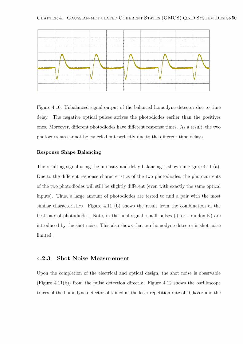
Chapter 4. Gaussian-modulated Coherent States (GMCS) QKD System Design50
Figure 4.10: Unbalanced signal output of the balanced homodyne detector due to time
delay. The negative optical pulses arrives the photodiodes earlier than the positives
ones. Moreover, different photodiodes have different response times. As a result, the two
photocurrents cannot be canceled out perfectly due to the different time delays.
Response Shape Balancing
The resulting signal using the intensity and delay balancing is shown in Figure 4.11 (a).
Due to the different response characteristics of the two photodiodes, the photocurrents
of the two photodiodes will still be slightly different (even with exactly the same optical
inputs). Thus, a large amount of photodiodes are tested to find a pair with the most
similar characteristics. Figure 4.11 (b) shows the result from the combination of the
best pair of photodiodes. Note, in the final signal, small pulses (+ or - randomly) are
introduced by the shot noise. This also shows that our homodyne detector is shot-noise
limited.
4.2.3 Shot Noise Measurement
Upon the completion of the electrical and optical design, the shot noise is observable
(Figure 4.11(b)) from the pulse detection directly. Figure 4.12 shows the oscilloscope
traces of the homodyne detector obtained at the laser repetition rate of 100kHz and the
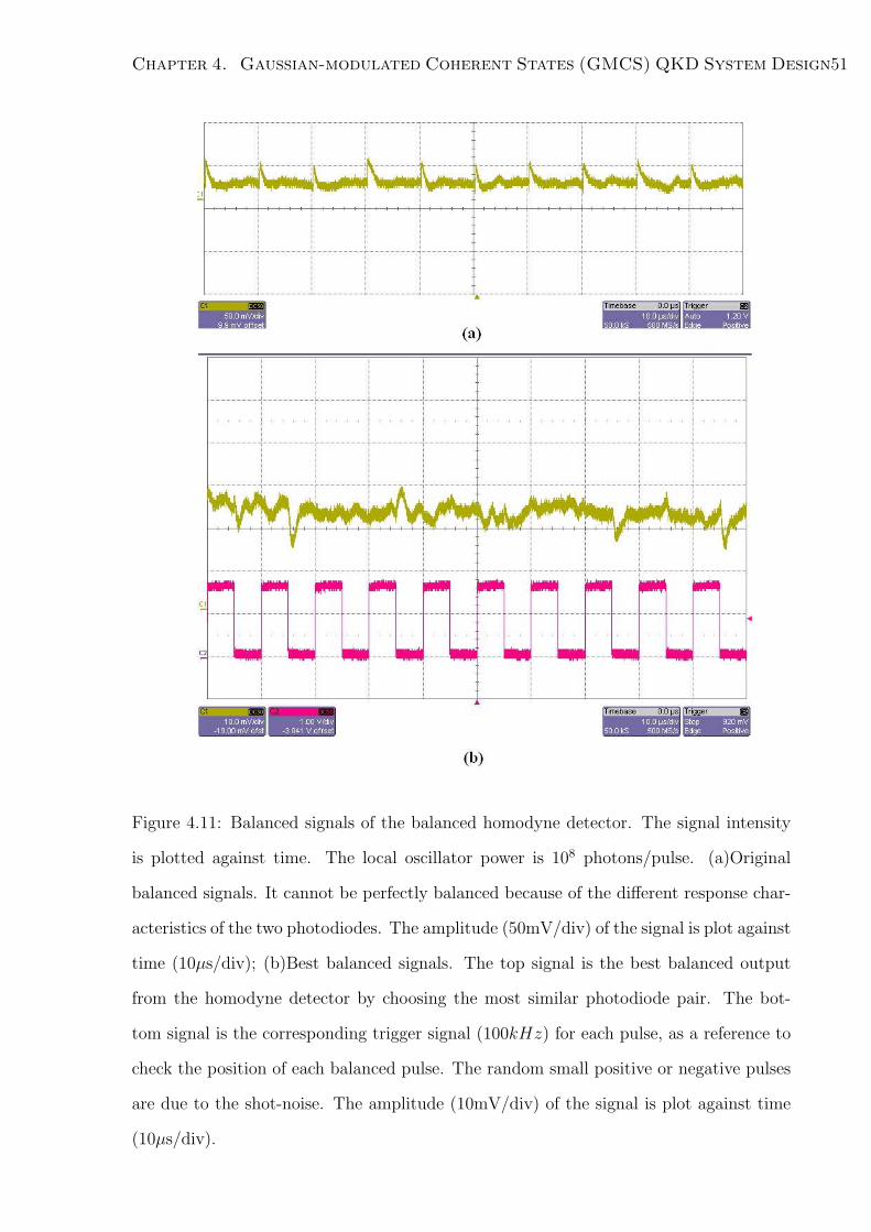
Chapter 4. Gaussian-modulated Coherent States (GMCS) QKD System Design51
Figure 4.11: Balanced signals of the balanced homodyne detector. The signal intensity
is plotted against time. The local oscillator power is 108 photons/pulse. (a)Original
balanced signals. It cannot be perfectly balanced because of the different response char-
acteristics of the two photodiodes. The amplitude (50mV/div) of the signal is plot against
time (10µs/div); (b)Best balanced signals. The top signal is the best balanced output
from the homodyne detector by choosing the most similar photodiode pair. The bot-
tom signal is the corresponding trigger signal (100kHz) for each pulse, as a reference to
check the position of each balanced pulse. The random small positive or negative pulses
are due to the shot-noise. The amplitude (10mV/div) of the signal is plot against time
(10µs/div).
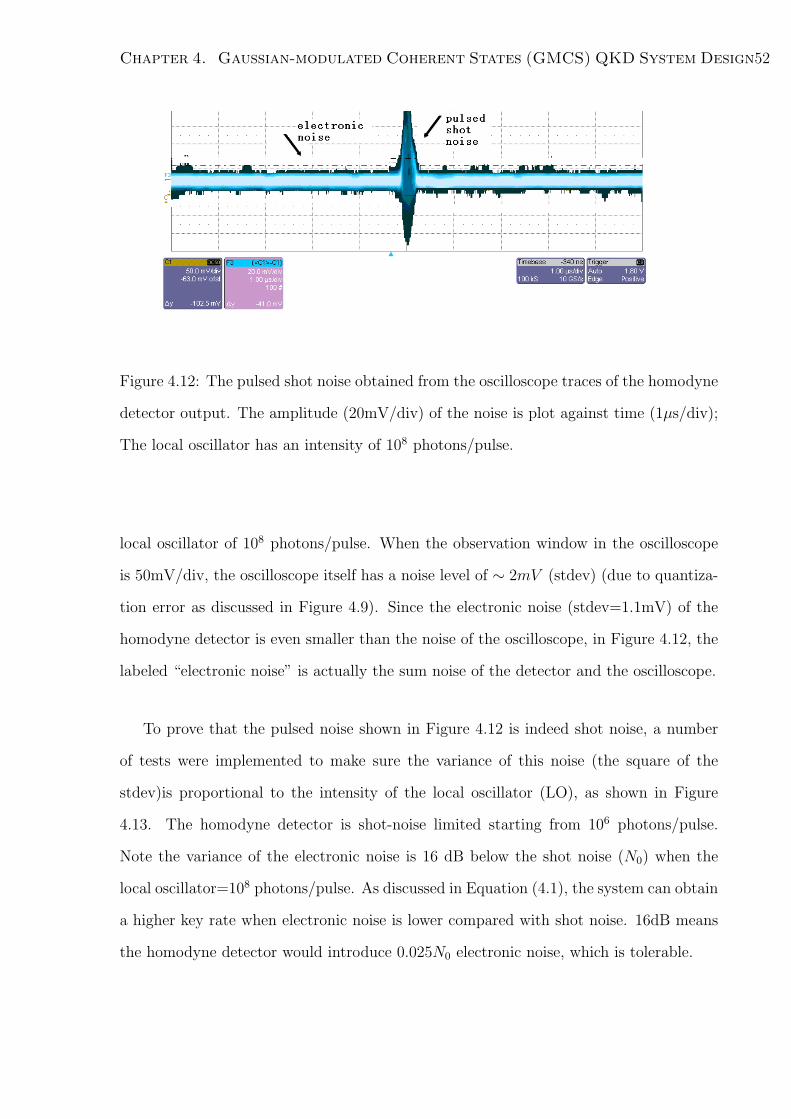
Chapter 4. Gaussian-modulated Coherent States (GMCS) QKD System Design52
Figure 4.12: The pulsed shot noise obtained from the oscilloscope traces of the homodyne
detector output. The amplitude (20mV/div) of the noise is plot against time (1µs/div);
The local oscillator has an intensity of 108 photons/pulse.
local oscillator of 108 photons/pulse. When the observation window in the oscilloscope
is 50mV/div, the oscilloscope itself has a noise level of ∼ 2mV (stdev) (due to quantiza-
tion error as discussed in Figure 4.9). Since the electronic noise (stdev=1.1mV) of the
homodyne detector is even smaller than the noise of the oscilloscope, in Figure 4.12, the
labeled “electronic noise” is actually the sum noise of the detector and the oscilloscope.
To prove that the pulsed noise shown in Figure 4.12 is indeed shot noise, a number
of tests were implemented to make sure the variance of this noise (the square of the
stdev)is proportional to the intensity of the local oscillator (LO), as shown in Figure
4.13. The homodyne detector is shot-noise limited starting from 106 photons/pulse.
Note the variance of the electronic noise is 16 dB below the shot noise (N0) when the
local oscillator=108 photons/pulse. As discussed in Equation (4.1), the system can obtain
a higher key rate when electronic noise is lower compared with shot noise. 16dB means
the homodyne detector would introduce 0.025N0 electronic noise, which is tolerable.

Chapter 4. Gaussian-modulated Coherent States (GMCS) QKD System Design53
Figure 4.13: Noise measurement of the balanced homodyne detector. The variance of
the noise changes linearly with the intensity of the local oscillator. When the intensity of
the local oscillator is less than less 105 photons/pulse, the electronic noise is dominating.
After that, the detector is shot-noise limited and for 108 photons/pulse, the variance of
shot noise is 16dB higher than the electronic noise.
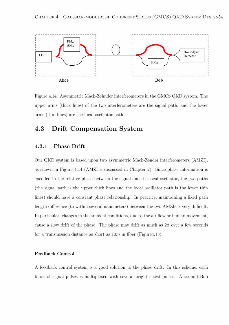
Chapter 4. Gaussian-modulated Coherent States (GMCS) QKD System Design54
Figure 4.14: Asymmetric Mach-Zehnder interferometers in the GMCS QKD system. The
upper arms (thick lines) of the two interferometers are the signal path, and the lower
arms (thin lines) are the local oscillator path.
4.3 Drift Compensation System
4.3.1 Phase Drift
Our QKD system is based upon two asymmetric Mach-Zender interferometers (AMZI),
as shown in Figure 4.14 (AMZI is discussed in Chapter 2). Since phase information is
encoded in the relative phase between the signal and the local oscillator, the two paths
(the signal path is the upper thick lines and the local oscillator path is the lower thin
lines) should have a constant phase relationship. In practice, maintaining a fixed path
length difference (to within several nanometers) between the two AMZIs is very difficult.
In particular, changes in the ambient conditions, due to the air flow or human movement,
cause a slow drift of the phase. The phase may drift as much as 2π over a few seconds
for a transmission distance as short as 10m in fiber (Figure4.15).
Feedback Control
A feedback control system is a good solution to the phase drift. In this scheme, each
burst of signal pulses is multiplexed with several brighter test pulses. Alice and Bob
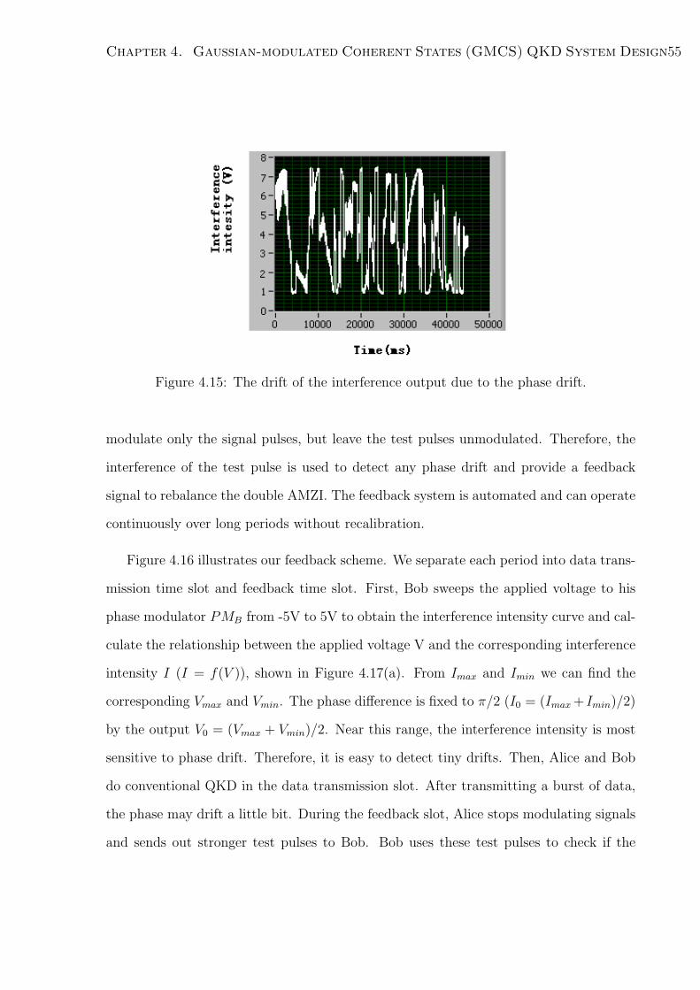
Chapter 4. Gaussian-modulated Coherent States (GMCS) QKD System Design55
Figure 4.15: The drift of the interference output due to the phase drift.
modulate only the signal pulses, but leave the test pulses unmodulated. Therefore, the
interference of the test pulse is used to detect any phase drift and provide a feedback
signal to rebalance the double AMZI. The feedback system is automated and can operate
continuously over long periods without recalibration.
Figure 4.16 illustrates our feedback scheme. We separate each period into data trans-
mission time slot and feedback time slot. First, Bob sweeps the applied voltage to his
phase modulator PMB from -5V to 5V to obtain the interference intensity curve and cal-
culate the relationship between the applied voltage V and the corresponding interference
intensity I (I = f(V )), shown in Figure 4.17(a). From Imax and Imin we can find the
corresponding Vmax and Vmin. The phase difference is fixed to π/2 (I0 = (Imax + Imin)/2)
by the output V0 = (Vmax + Vmin)/2. Near this range, the interference intensity is most
sensitive to phase drift. Therefore, it is easy to detect tiny drifts. Then, Alice and Bob
do conventional QKD in the data transmission slot. After transmitting a burst of data,
the phase may drift a little bit. During the feedback slot, Alice stops modulating signals
and sends out stronger test pulses to Bob. Bob uses these test pulses to check if the
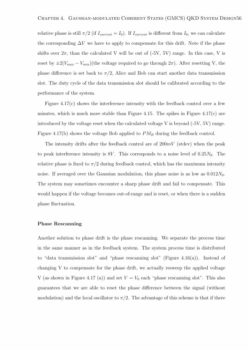
Chapter 4. Gaussian-modulated Coherent States (GMCS) QKD System Design56
relative phase is still π/2 (if Icurrent = I0). If Icurrent is different from I0, we can calculate
the corresponding ∆V we have to apply to compensate for this drift. Note if the phase
shifts over 2π, than the calculated V will be out of (-5V, 5V) range. In this case, V is
reset by ±2(Vmax − Vmin)(the voltage required to go through 2π). After resetting V, the
phase difference is set back to π/2, Alice and Bob can start another data transmission
slot. The duty cycle of the data transmission slot should be calibrated according to the
performance of the system.
Figure 4.17(c) shows the interference intensity with the feedback control over a few
minutes, which is much more stable than Figure 4.15. The spikes in Figure 4.17(c) are
introduced by the voltage reset when the calculated voltage V is beyond (-5V, 5V) range.
Figure 4.17(b) shows the voltage Bob applied to PMB during the feedback control.
The intensity drifts after the feedback control are of 200mV (stdev) when the peak
to peak interference intensity is 8V . This corresponds to a noise level of 0.25N0. The
relative phase is fixed to π/2 during feedback control, which has the maximum intensity
noise. If averaged over the Gaussian modulation, this phase noise is as low as 0.012N0.
The system may sometimes encounter a sharp phase drift and fail to compensate. This
would happen if the voltage becomes out-of-range and is reset, or when there is a sudden
phase fluctuation.
Phase Rescanning
Another solution to phase drift is the phase rescanning. We separate the process time
in the same manner as in the feedback system. The system process time is distributed
to “data transmission slot” and “phase rescanning slot” (Figure 4.16(a)). Instead of
changing V to compensate for the phase drift, we actually resweep the applied voltage
V (as shown in Figure 4.17 (a)) and set V = V0 each “phase rescanning slot”. This also
guarantees that we are able to reset the phase difference between the signal (without
modulation) and the local oscillator to π/2. The advantage of this scheme is that if there
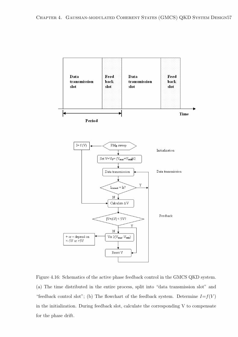
Chapter 4. Gaussian-modulated Coherent States (GMCS) QKD System Design57
Figure 4.16: Schematics of the active phase feedback control in the GMCS QKD system.
(a) The time distributed in the entire process, split into “data transmission slot” and
“feedback control slot”; (b) The flowchart of the feedback system. Determine I=f(V )
in the initialization. During feedback slot, calculate the corresponding V to compensate
for the phase drift.
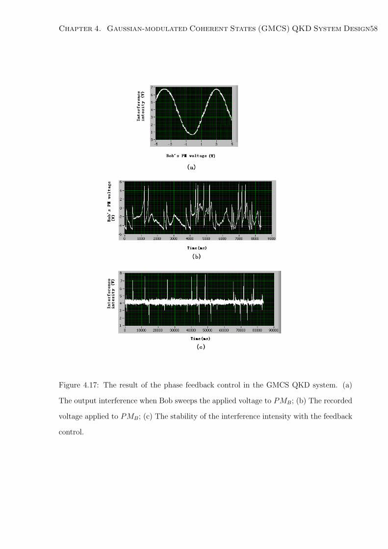
Chapter 4. Gaussian-modulated Coherent States (GMCS) QKD System Design58
Figure 4.17: The result of the phase feedback control in the GMCS QKD system. (a)
The output interference when Bob sweeps the applied voltage to PMB; (b) The recorded
voltage applied to PMB; (c) The stability of the interference intensity with the feedback
control.

Chapter 4. Gaussian-modulated Coherent States (GMCS) QKD System Design59
is a sudden flip in the phase, it can still be compensated. Moreover, in this case, the
control voltage would never exceed the (-5V, 5V) range, and can reduce the shape phase
drifts in Figure 4.17(c). The disadvantage of this scheme is that it decreases the duty
cycle of the data transmission slot, due to the longer phase rescanning time.
4.3.2 Polarization Drift
Polarization drift also introduces instability to the interference signal. One straightfor-
ward solution to polarization drift in the two AMZIs is to use polarization maintaining
(PM) fiber. A computer-controlled polarization controller can also be used. To test the
polarization drift, we can measure the output intensity drift from the polarization beam
splitter. From our preliminary test, as shown in Figure 4.18(a), there is no rapid fluctu-
ation in polarization . Moreover, the polarization can be stable for over hours (Figure
4.18(b) for 1000s). In this case, the polarization can be considered as stable within the
key distribution time. For practice implementation in the future, the polarization drift
problem still has to be solved by using PM fiber or active polarization compensation.
4.4 Frequency-multiplexing
One of the significant problems in the previous continuous-variable QKD demonstrations
is the crosstalk between the local oscillator and the signal [27] [34]. Typically, there is a
60dB intensity difference between the local oscillator and the signal pulses. In [27] [34],
separate channels are used to transmit the local oscillator and the signal. This is not
practical over long distances because it is difficult to maintain constant polarization and
phase in two different channels, especially in fiber.
Conventionally, there are two ways to separate the signal and the local oscillator:
time-multiplexing and polarization-multiplexing. For time-multiplexing, as shown in
Figure 4.19, the signal travels through the shorter (upper) arm in Alice’s AMZI, while

Chapter 4. Gaussian-modulated Coherent States (GMCS) QKD System Design60
Figure 4.18: Polarization drifts in the GMCS QKD system. The intensity (V) is the
output from polarization beam splitter. (a) The polarization stability for a short time
(0.1s); (b) The polarization stability for a short time (1000s).
Chapter 4. Gaussian-modulated Coherent States (GMCS) QKD System Design61
Figure 4.19: Schematics of time-multiplexing in GMCS QKD system. The signal and
the local oscillator are separated in time domain by using asymmetrical Mach-Zehnder
interferometers.
the local oscillator travels through the longer (lower) arm. In this case, the transmitted
signal and the local oscillator are separated in time domain. However, the fiber length
difference in Alice’s AMZI should be long enough to separate the signal and the local
oscillator. For example, for a 100ns pulse, the fiber length difference should be at least
20m. This long path difference will result in an unstable AMZI. To have less fiber length
difference, the pulse width should be narrow. But narrow pulses require higher laser
power to obtain 108photons/pulse local oscillator (in our setup, a 1ns local oscillator
needs a 50mW laser).
Limited by the power of our cw laser (10mW maximum), we turned to polarization-
multiplexing. The typical polarization extinction ratio of the polarization beam splitter
(PBS) is 20-30dB. This is not enough to separate the signal and the local oscillator
with an intensity difference of 60dB. The poor extinction ratio yields high crosstalk and
therefore a high error rate.
We proposed a unique frequency-multiplexing scheme to separate the signal and the
local oscillator. As illustrated in Figure 4.20, on Alice’s side, the signal’s frequency is
shifted while the local oscillator is un-shifted. On Bob’s side, before the signal and the
local oscillator are brought together to interfere at the coupler, the local oscillator’s fre-

Chapter 4. Gaussian-modulated Coherent States (GMCS) QKD System Design62
Figure 4.20: Schematics of frequency-multiplexing in GMCS QKD. The upper (thicker)
arms are the signal arms, the lower (thinner) arms are the local oscillator arms. The
local oscillator leakage will go through lower arm on Alice and upper arm on Bob and
have no frequency shift.
quency is shifted while the signal is not. Consequently, the signal and the local oscillator
will have the same frequency at the coupler. The reason we shift signal’s frequency first
is to reduce the insertion loss of signal arm on Bob’s side. The leakage of the local os-
cillator in the signal path has a different frequency because it is not frequency shifted
at all. Acousto-optic modulators (AOMs) are used as frequency shifters in our system.
The two AOMs have an identical frequency shift of 55MHz. The local oscillator and
the signal will have the same frequency and interfere with each other while the local
oscillator and its leakage will have a 55MHz frequency difference. Because 55MHz is
a small frequency compared with optical frequency, the local oscillator and its leakage
produce an interference beat at 55MHz. Due to the low frequency response range of the
homodyne detector, the 55MHz beat signal is automatically filtered out.
4.5 Initialization Procedure
In the GMCS system design shown in Figure 4.2, there are 5 polarization controllers. Two
polarization controllers are used for the polarization adjustment in the AMZIs due to the
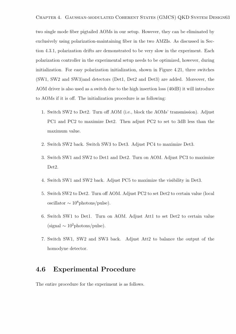
Chapter 4. Gaussian-modulated Coherent States (GMCS) QKD System Design63
two single mode fiber pigtailed AOMs in our setup. However, they can be eliminated by
exclusively using polarization-maintaining fiber in the two AMZIs. As discussed in Sec-
tion 4.3.1, polarization drifts are demonstrated to be very slow in the experiment. Each
polarization controller in the experimental setup needs to be optimized, however, during
initialization. For easy polarization initialization, shown in Figure 4.21, three switches
(SW1, SW2 and SW3)and detectors (Det1, Det2 and Det3) are added. Moreover, the
AOM driver is also used as a switch due to the high insertion loss (40dB) it will introduce
to AOMs if it is off. The initialization procedure is as following:
1. Switch SW2 to Det2. Turn off AOM (i.e., block the AOMs’ transmission). Adjust
PC1 and PC2 to maximize Det2. Then adjust PC2 to set to 3dB less than the
maximum value.
2. Switch SW2 back. Switch SW3 to Det3. Adjust PC4 to maximize Det3.
3. Switch SW1 and SW2 to Det1 and Det2. Turn on AOM. Adjust PC3 to maximize
Det2.
4. Switch SW1 and SW2 back. Adjust PC5 to maximize the visibility in Det3.
5. Switch SW2 to Det2. Turn off AOM. Adjust PC2 to set Det2 to certain value (local
oscillator ∼ 108photons/pulse).
6. Switch SW1 to Det1. Turn on AOM. Adjust Att1 to set Det2 to certain value
(signal ∼ 102photons/pulse).
7. Switch SW1, SW2 and SW3 back. Adjust Att2 to balance the output of the
homodyne detector.
4.6 Experimental Procedure
The entire procedure for the experiment is as follows.

Chapter 4. Gaussian-modulated Coherent States (GMCS) QKD System Design64
Figure 4.21: GMCS QKD system. Laser-1550nm cw laser diode; PC-polarization con-
troller; AM-amplitude modulator; PBS-polarizing beam splitters; AM&PM-amplitude
and phase modulator; AOM- acusto-optical modulator; SW- optical switch; VOA- vari-
able optical attenuator; Det- detector; PM-phase modulator; SM Coupler: single mode
coupler; ODL- variable optical delay line; Homodyne- homodyne detector.
Chapter 4. Gaussian-modulated Coherent States (GMCS) QKD System Design65
1. Initialization.
2. Alice sends out strong test pulses to control relative phase between the local oscil-
lator and the signal arms.
3. Start data transmission. Each burst of signals includes synchronization data and
real data. For real data, Alice generates two independent sets of Gaussian distribu-
tion random numbers x (amplitude quadrature) and p (phase quadrature). Convert
the numbers into their corresponding voltages applied to AM&PM, i.e., encode into
sequence of |x + ip > signal pulses, and sends them to Bob.
4. Bob randomly applies amplitude or phase quadrature measurement by choosing 0
or π/2 phase modulation on the local oscillator arm.
5. After transmission, Bob informs Alice which quadrature he measured through an
authenticated public channel. Alice drops irrelevant data, publicly compare a ran-
dom sample of their relevant key and proceed to data post-processing to distill
secret key.
4.7 Summary
In this chapter, we have designed the system configuration for the GMCS QKD system.
Starting from the simplest architecture, control systems and components are added to
solve the proposed challenges and problems. Compared with the previous GMCS QKD
demonstration [27][34][35], our system is a complete fiber-based system with one way
configuration and is able to demonstrate real key transmission over a long distance.
Chapter 5
Gaussian-modulated Coherent
States QKD System Results
This chapter presents the experimental results of our Gaussian-modulated coherent state
(GMCS) QKD system. This is the first demonstration of fiber-based one-way GMCS
QKD system over a large distance (5km).
5.1 System Results
Figure 5.1 illustrates our entire experimental setup, including the optical setup and the
electrical equipment. Alice first generates 100ns wide pulses (Figure 5.2) from a contin-
uous wave laser diode emitting at a wavelength of 1550 nm with an amplitude modu-
lator, driven by a function generator. The repetition rate is set to be 100kHz. These
pulses go into the polarization beam splitter (PBS) and are split into the strong lo-
cal oscillator pulses (typically 108 photons/pulse) and the weak signal pulses (typically
100 photons/pulse). For Gaussian-modulated coherent state QKD protocol, the required
modulation is a two dimensional Gaussian distribution centered on zero, with a customiz-
able variance VA, which is typically set to ≈ 40N0. To ensure the security of the system,
random Gaussian distribution numbers are required. However, computers can only gen-
66
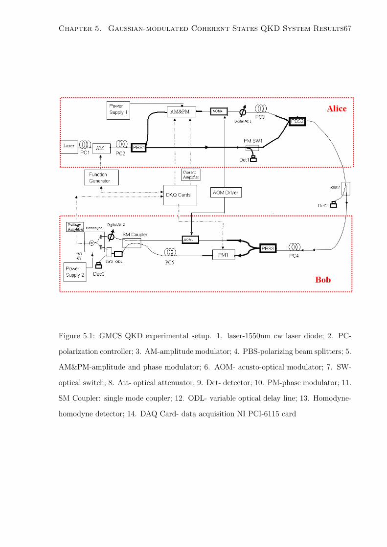
Chapter 5. Gaussian-modulated Coherent States QKD System Results67
Figure 5.1: GMCS QKD experimental setup. 1. laser-1550nm cw laser diode; 2. PC-
polarization controller; 3. AM-amplitude modulator; 4. PBS-polarizing beam splitters; 5.
AM&PM-amplitude and phase modulator; 6. AOM- acusto-optical modulator; 7. SW-
optical switch; 8. Att- optical attenuator; 9. Det- detector; 10. PM-phase modulator; 11.
SM Coupler: single mode coupler; 12. ODL- variable optical delay line; 13. Homodyne-
homodyne detector; 14. DAQ Card- data acquisition NI PCI-6115 card

Chapter 5. Gaussian-modulated Coherent States QKD System Results68
Figure 5.2: The experimental pulses generated by amplitude modulator (AM) on Alice’s
side.
erate pseudo-random numbers. In our experiment, a physical quantum random number
generator is used to generate a uniform distribution. Then the Box-Muller method [42]
is used to convert the uniform distribution to the Gaussian distribution. The encoding x
and p Gaussian distributed random numbers used in our experiment is plotted in Figure
5.3. Details are explained in Appendix A.
Acousto-optical modulators (AOMs) are used to overcome the crosstalk between the
local oscillator and the signal. The original laser power must be 10mW at the output
to compensate for various losses in the local oscillator paths. Signal pulses are contin-
uously modulated in amplitude and phase with a computer-driven electro-optics ampli-
tude&phase modulator. The shot noise variance N0 is used as a reference for all noise
levels for the remainder of the following calculations. The transmission fiber distance
between Alice and Bob is 5km. On Bob’s side, the weak signal and the local oscillator
are separated by a PBS, and interfere with each other. Bob’s phase modulator is used to
randomly choose x or p quadrature to measure. The quadrature signal is measured by
the homodyne detector.

Chapter 5. Gaussian-modulated Coherent States QKD System Results69
Figure 5.3: Alice’s two independent Gaussian distributed random numbers (x and p). In
the Box-Muller method, mean=0 and VA = 40 are used to generate Gaussian distributed
random numbers x and p. But the actually generated x and p have variances of Vx = 40.38
and Vp = 40.42 in the experiment.
As discussed in Chapter 4, the information rates for GMCS QKD system are derived
by:
∆I = IAB − IBE
IAB =1
2log2
ηGVA + 1 + ηGε
1 + ηGε
ImaxBE =
1
2log2
ηGVA + 1 + ηGε
η/[1−G + Gε + G/(VA + 1)] + 1− η
(5.1)
expressed in bits/symbol.
Here IAB is the mutual information between Bob and Alice. ImaxBE is the maximum
correlated information between Bob and Eve. G is the channel transmission; V is the
variance of Alice’s field quadratures in shot-noise units (V = VA + 1). η represents the
efficiency of the homodyne detector; ε is the “excess noise” due to the imperfections of
the components.
From Equation (5.1), in order to calculate the key rate, we need the values of G, η,
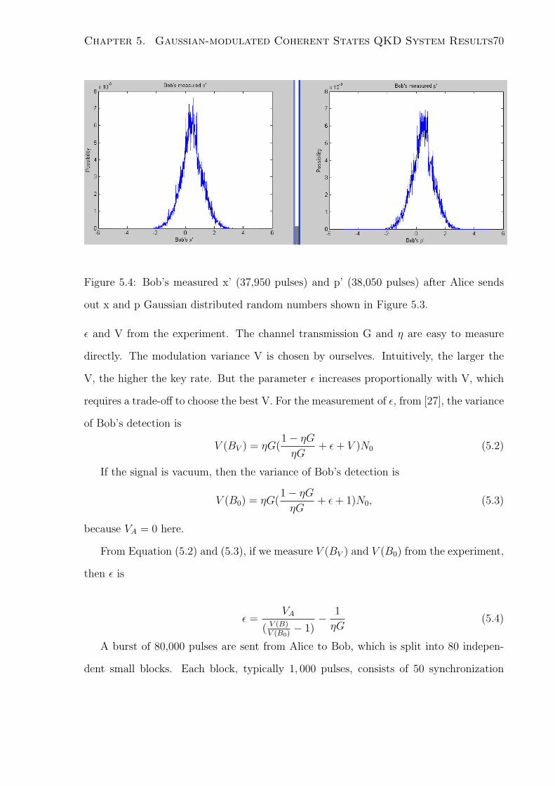
Chapter 5. Gaussian-modulated Coherent States QKD System Results70
Figure 5.4: Bob’s measured x’ (37,950 pulses) and p’ (38,050 pulses) after Alice sends
out x and p Gaussian distributed random numbers shown in Figure 5.3.
ε and V from the experiment. The channel transmission G and η are easy to measure
directly. The modulation variance V is chosen by ourselves. Intuitively, the larger the
V, the higher the key rate. But the parameter ε increases proportionally with V, which
requires a trade-off to choose the best V. For the measurement of ε, from [27], the variance
of Bob’s detection is
V (BV ) = ηG(1− ηG
ηG+ ε + V )N0 (5.2)
If the signal is vacuum, then the variance of Bob’s detection is
V (B0) = ηG(1− ηG
ηG+ ε + 1)N0, (5.3)
because VA = 0 here.
From Equation (5.2) and (5.3), if we measure V (BV ) and V (B0) from the experiment,
then ε is
ε =VA
( V (B)V (B0)
− 1)− 1
ηG(5.4)
A burst of 80,000 pulses are sent from Alice to Bob, which is split into 80 indepen-
dent small blocks. Each block, typically 1, 000 pulses, consists of 50 synchronization

Chapter 5. Gaussian-modulated Coherent States QKD System Results71
pulses and 950 data pulses. These synchronization pulses can also be used to estimate
the channel parameters (gain, excess noise and relative phase). The total 76,000 data
pulses are analyzed during testing. 37,950 of them are measured in x quadrature while
38,050 of them are measured in p quadrature. Figure 5.4 shows the measured x’ (37,950
data points) and p’ (38,050 data points) on Bob’s side and the corresponding x and p
on Alice’s side are shown in Figure 5.3. The output noise on Bob’s side is due to four
contributions: the channel noise Nchan, the noise introduced by the electrical noise, the
imperfect efficiency of the homodyne detector, and other technical imperfections (such as
the pulse modulation noises and the laser phase noises). Figure 5.5 illustrates the corre-
lation between Bob’s measurement results (x’ and p’) and Alice’s encoding information
(x and p).
With a 5km fiber between Alice and Bob, the measured Vx(BV )=0.401, Vx(B0) =
0.0430 and Vp(BV ) = 0.392, Vp(B0) = 0.0421. Therefore, Vx(BV )/Vx(B0) = 9.33 and
Vp(BV )/Vp(B0) = 9.31. Since in our experimental setup η=0.277 (the efficiency of ho-
modyne detector itself is 56%, and the insertion loss of all the components on Bob’s side
is 45%), G=0.794, and variance of the corresponding xA and pA is 40.3 and 40.2, from
Equation (5.4), εx = 0.299 and εp = 0.305. Then, from Equation (5.1), we are able to
achieve 0.155 bits/pulse. With a repetition rate of 100kHz, the key rate is 15.5kbits/s.
Given this raw available secret information rate, the secret bits still have to be ex-
tracted from the Gaussian data using a “sliced reconciliation” algorithm [32] with a
current efficiency of 0.7. The key information leaked out to Eve is finally removed by a
standard privacy amplification procedure.
5.2 Summary
Compared with previous demonstrations, our setup is the first one-way fiber-based GMCS
QKD system over a long distance. Our system is relatively stable due to the phase
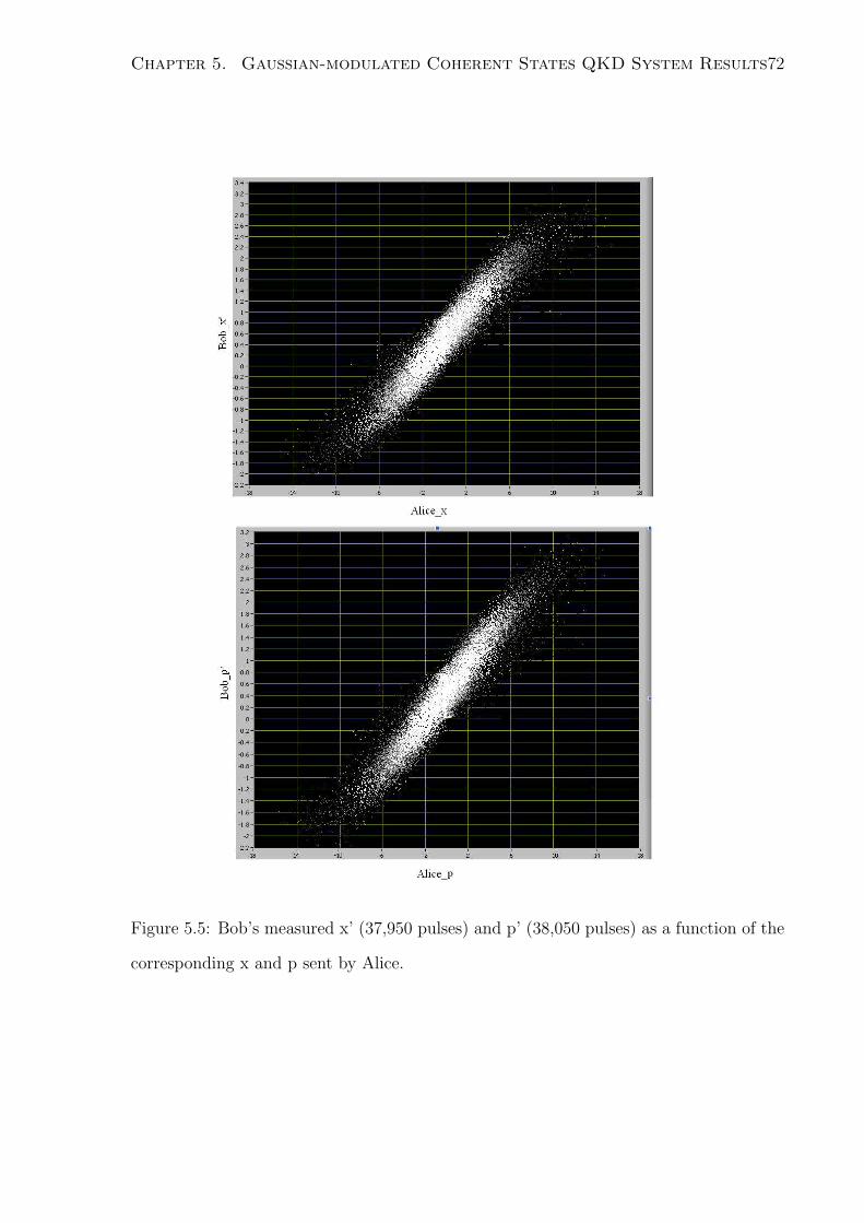
Chapter 5. Gaussian-modulated Coherent States QKD System Results72
Figure 5.5: Bob’s measured x’ (37,950 pulses) and p’ (38,050 pulses) as a function of the
corresponding x and p sent by Alice.

Chapter 5. Gaussian-modulated Coherent States QKD System Results73
feedback control and the entire setup does not need to be isolated from the external
perturbations. We used frequency-multiplexing to make the strong local oscillator and
weak signal to travel through the same fiber channel of 5km.

Chapter 6
Conclusions
Experimental quantum key distribution has made tremendous developments over the
past few years. In this thesis, we have demonstrated two practical QKD systems over
long telecom fiber: Sagnac loop QKD and Gaussian-modulated coherent states QKD.
The results show that our systems offer better system performances than the previous
works [20] [23] [27] [34] [35].
6.1 Contributions
A stable Sagnac QKD system over 40km fiber loop was demonstrated in Chapter 3.
The advantage of the Sagnac QKD is its automatic phase compensation and its ease
of implementation in the future quantum networks. Compared with the most recent
demonstration (Table 6.1), our Sagnac QKD system has simpler configuration, higher
visibility, and more stable performance, with the use of polarization-insensitive phase
modulators. A lower quantum bit error rate (QBER) of 3 − 5% was achieved with a
repetition rate of 22.7kHz and the system can be stable for over one hour without any
recalibration .
The QKD system based on Gaussian-modulated coherent state (GMCS) was discussed
in Chapter 4 and Chapter 5. GMCS QKD is proposed as a potential solution to increase
74
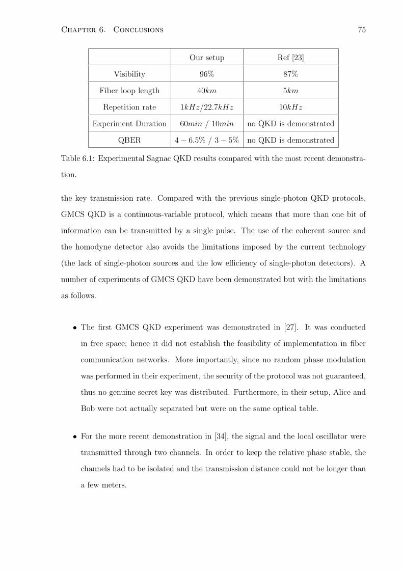
Chapter 6. Conclusions 75
Our setup Ref [23]
Visibility 96% 87%
Fiber loop length 40km 5km
Repetition rate 1kHz/22.7kHz 10kHz
Experiment Duration 60min / 10min no QKD is demonstrated
QBER 4− 6.5% / 3− 5% no QKD is demonstrated
Table 6.1: Experimental Sagnac QKD results compared with the most recent demonstra-
tion.
the key transmission rate. Compared with the previous single-photon QKD protocols,
GMCS QKD is a continuous-variable protocol, which means that more than one bit of
information can be transmitted by a single pulse. The use of the coherent source and
the homodyne detector also avoids the limitations imposed by the current technology
(the lack of single-photon sources and the low efficiency of single-photon detectors). A
number of experiments of GMCS QKD have been demonstrated but with the limitations
as follows.
• The first GMCS QKD experiment was demonstrated in [27]. It was conducted
in free space; hence it did not establish the feasibility of implementation in fiber
communication networks. More importantly, since no random phase modulation
was performed in their experiment, the security of the protocol was not guaranteed,
thus no genuine secret key was distributed. Furthermore, in their setup, Alice and
Bob were not actually separated but were on the same optical table.
• For the more recent demonstration in [34], the signal and the local oscillator were
transmitted through two channels. In order to keep the relative phase stable, the
channels had to be isolated and the transmission distance could not be longer than
a few meters.
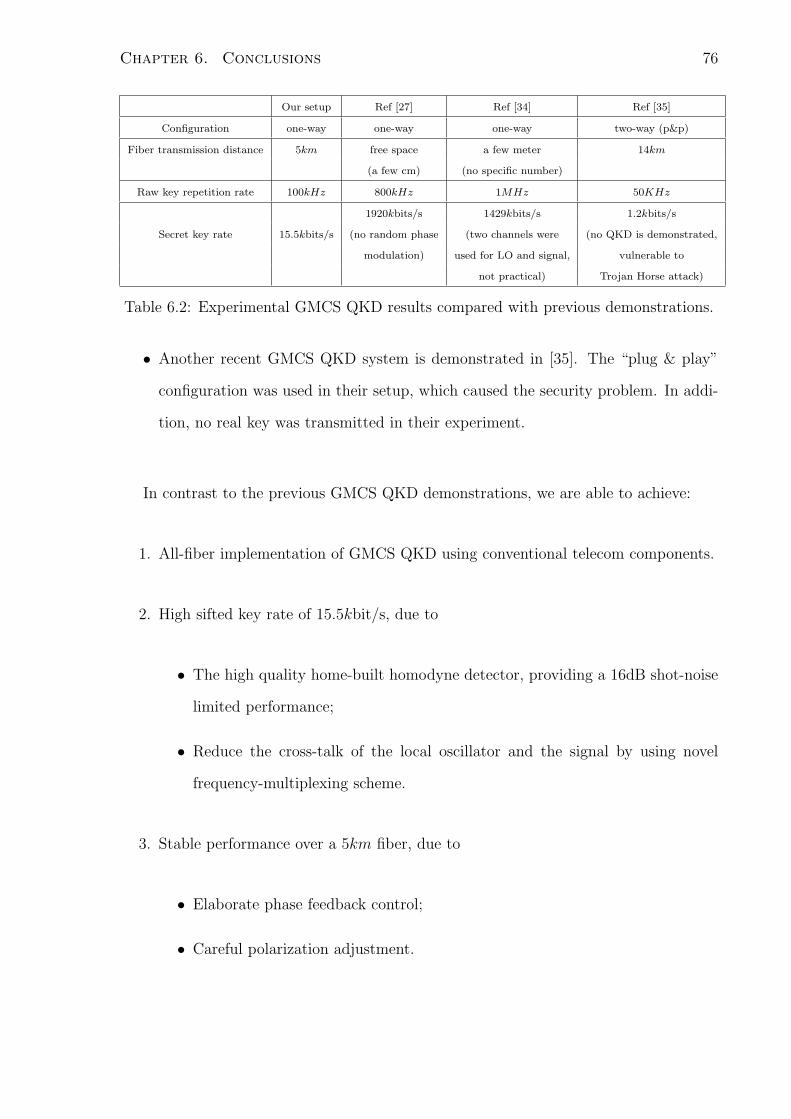
Chapter 6. Conclusions 76
Our setup Ref [27] Ref [34] Ref [35]
Configuration one-way one-way one-way two-way (p&p)
Fiber transmission distance 5km free space a few meter 14km
(a few cm) (no specific number)
Raw key repetition rate 100kHz 800kHz 1MHz 50KHz
1920kbits/s 1429kbits/s 1.2kbits/s
Secret key rate 15.5kbits/s (no random phase (two channels were (no QKD is demonstrated,
modulation) used for LO and signal, vulnerable to
not practical) Trojan Horse attack)
Table 6.2: Experimental GMCS QKD results compared with previous demonstrations.
• Another recent GMCS QKD system is demonstrated in [35]. The “plug & play”
configuration was used in their setup, which caused the security problem. In addi-
tion, no real key was transmitted in their experiment.
In contrast to the previous GMCS QKD demonstrations, we are able to achieve:
1. All-fiber implementation of GMCS QKD using conventional telecom components.
2. High sifted key rate of 15.5kbit/s, due to
• The high quality home-built homodyne detector, providing a 16dB shot-noise
limited performance;
• Reduce the cross-talk of the local oscillator and the signal by using novel
frequency-multiplexing scheme.
3. Stable performance over a 5km fiber, due to
• Elaborate phase feedback control;
• Careful polarization adjustment.
Chapter 6. Conclusions 77
6.2 Future Work
6.2.1 Sagnac Loop QKD System
The results of our Sagnac QKD system are not stunning, but it demonstrates the fea-
sibility of Sagnac Loop QKD using polarization-insensitive phase modulators. 22.7kHz
is the highest repetition rate with the current setup and equipment. The major limiting
factor is the response rate of the AOM drivers. If the AOM drivers are replaced, the
next obstacle would be the AOMs themselves, with a response rate of about 2MHz. In
addition, the single-photon detectors can only operate around several MHz. Hence a
realistic goal for this implementation is on the order of a few MHz and our next step is
to improve the repetition rate to 1MHz.
Another improvement is to achieve a long-term stability. A computer-controlled po-
larization controller can be used for active compensation over long periods of time. By
sending test pulses, Bob can get feedback in polarization states and the synchronization
signals. These test pulses can be sent either in time domain or frequency domain.
In addition to the performance improvement, the system setup can also be used to
demonstrate protocols other than BB84. As mentioned in Chapter 3, the transmittance
of the AOM changes with the amplitude of the driving signal, which makes it possible
to modulate the amplitude as well as the phase. In this case, decoy state QKD [13]
and continuous-variable GMCS QKD can take advantage of the polarization-insensitive
amplitude and phase modulator.
Quantum network is an interesting and promising topic in recent years. Sagnac QKD
system is ideal for the implementation of ring QKD networks. Each user in the Sagnac
loop QKD network can communicate with others by simply adding one phase modulator,
as discussed in Chapter3 (Figure3.9). It would be exciting if we could demonstrate the
QKD ring network with our Sagnac QKD system. In addition, though the security of
one-way QKD has been proven, a two-way QKD is open to many more attacks. Further
Chapter 6. Conclusions 78
theoretical analysis is still required in the future.
6.2.2 GMCS QKD System
Our current GMCS system is able to achieve 15.5kbits/s secret key rate. It is determined
by the key generation rate of 0.155 bit/pulse and 100kHz repetition rate. In order to
achieve higher key rate per pulse, we should eliminate the excess noise by upgrading the
equipment and isolating the optical system from external perturbations. The total key
rate can also be increased by having a higher repetition rate, which is primarily limited
by the sampling rate of the data acquisition (DAQ) card and the response time of the
homodyne detector. The DAQ card (10MS/s) can be replaced with a high speed field
programmable gate array (FPGA). For the homodyne detector, the high and low pass
filters in the electrical amplifier circuit can be improved to achieve a higher repetition
rate.
Another problem is to maintain the stability of the system. Currently, without proper
shielding, the phase drifts a 2π every few seconds. This limits our data transmission block
size to 1,000 pulses at 100kHz repetition rate. This means that we compensate for the
phase every 10ms. If we can avoid the air flow, the period of phase drifts can be extended
to several minutes, which would increase the block size significantly.
The security proof of GMCS QKD protocol against general attacks is an open question
to date. Further security issues must be studied in the future. Although the continuous-
variable pulses in GMCS QKD allow more than 1bit information per pulse, the total
efficiency of current experimental GMCS QKD is still not high enough. Improvements in
the protocol as well as the data post-processing algorithms are still required. Moreover,
the transmission distance of the GMCS QKD system is limited to dozens of kilometers
so far. In this case, it is necessary to do further research in both theory and practice to
develop the realistic limitations on the GMCS QKD protocol.
Chapter 6. Conclusions 79
6.3 Summary
Two experimental QKD systems are demonstrated in this thesis. The Sagnac QKD
system with polarization-insensitive phase modulators leads to a better performance and
is feasible for future QKD network setup. Our GMCS QKD is the first fiber-based one-
way demonstration over a long fiber distance.
Security is so important in our society that we cannot risk compromising it, even
when code breaking is extremely unlikely. Quantum cryptography is the only known way
to achieve absolute security in key distribution, and therefore will become an important
technology in the future. The long-distance QKD systems demonstrated in this thesis
have paved the path to future deployment of quantum cryptosystems, enabling pervasive,
secure, quantum communication networks.
Appendix A
Gaussian distribution random
number generation
The objective of this part is to generate the two Gaussian distribution random number
(mean=0 and variance=VA) sets x and p, and convert them into the encoding amplitude
(A) and phase (Φ) on Alice’s side.
To ensure the security of the system, truly random Gaussian distribution numbers
are required. However, computers can only generate pseudo-random numbers. In our
experiment, a physical quantum random number generator is used to generate a uniform
distribution. Then the Box-Muller Method is used to convert the uniform distribution
to Gaussian distribution.
A.1 Quantum Random Number Generator
Although random numbers are required in many applications, their generation is often
overlooked. Being deterministic, computers are not capable of producing random num-
bers. A physical source of randomness is necessary. Quantum physics being intrinsically
random, it is natural to exploit a quantum process for such a source.
Quantis (from id quantique) is used as the physical random number generator in our
80
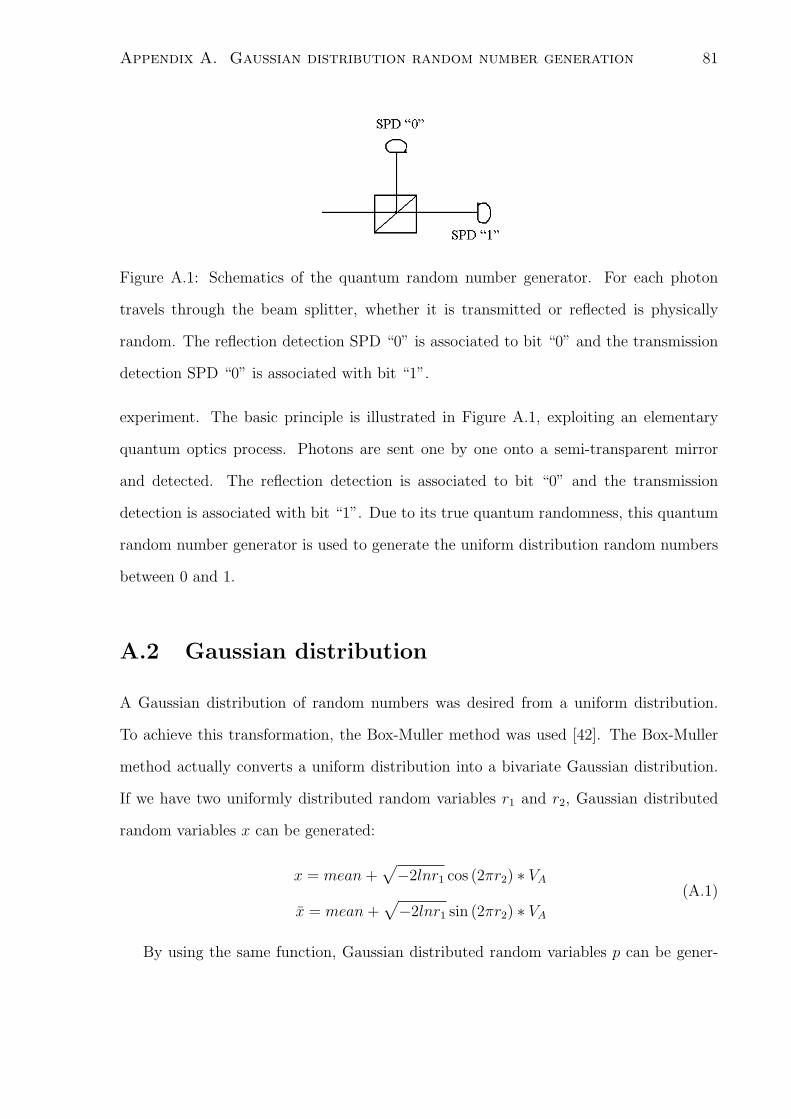
Appendix A. Gaussian distribution random number generation 81
Figure A.1: Schematics of the quantum random number generator. For each photon
travels through the beam splitter, whether it is transmitted or reflected is physically
random. The reflection detection SPD “0” is associated to bit “0” and the transmission
detection SPD “0” is associated with bit “1”.
experiment. The basic principle is illustrated in Figure A.1, exploiting an elementary
quantum optics process. Photons are sent one by one onto a semi-transparent mirror
and detected. The reflection detection is associated to bit “0” and the transmission
detection is associated with bit “1”. Due to its true quantum randomness, this quantum
random number generator is used to generate the uniform distribution random numbers
between 0 and 1.
A.2 Gaussian distribution
A Gaussian distribution of random numbers was desired from a uniform distribution.
To achieve this transformation, the Box-Muller method was used [42]. The Box-Muller
method actually converts a uniform distribution into a bivariate Gaussian distribution.
If we have two uniformly distributed random variables r1 and r2, Gaussian distributed
random variables x can be generated:
x = mean +√−2lnr1 cos (2πr2) ∗ VA
x̄ = mean +√−2lnr1 sin (2πr2) ∗ VA
(A.1)
By using the same function, Gaussian distributed random variables p can be gener-

Appendix A. Gaussian distribution random number generation 82
ated:
p = mean +√−2lnr3 cos (2πr4) ∗ VA
p̄ = mean +√−2lnr3 sin (2πr4) ∗ VA
(A.2)
where r3 and r4 are another two independent uniformly distributed random variables.
A.3 Amplitude and phase modulation
Although the Gaussian distribution was produced, this is not the form in which the
variables will be given to the AM&PM modulator. To achieve the amplitude and phase
modulation variables, a simple polar conversion was performed as follows.
We are given two random variables, x and p. The phase and amplitude is given by:
A =√
x2 + p2
Φ = arctan(p/x)
(A.3)
It is very important to note that the value of the arctangent must be in between -π/2
and 3π/2 to ensure proper conversion back to rectangular coordinates.

Bibliography
[1] W Diffie, M E Hellman, “Privacy and Authentication: An Introduction to Cryptog-
raphy”, in Proc. IEEE, 67(3), 397 (1979).
[2] R. L. Rivest, A. Shamir, and L. M. Adleman, “A method for obtaining digital signa-
tures and public-key cryptosystems”, Communications of the ACM 21(2), 120(1978).
[3] P. W. Shor, “Algorithms for Quantum Computation: Discrete Logarithms and Fac-
toring,” Proc. 35th Annual Symp. on Foundations of Computer Science, 124 (1994).
[4] C.E. Shannon, “One-Time Pads For Secure Communication In Ubiquitous”, Com-
munication theory of secrecy systems, Bell System Tech. J. 28 (1949).
[5] Wiesner, S., “Conjugate coding”, Sigact News 15(1),78(1983); original manuscript
written circa 1970.
[6] C. H. Bennett and G. Brassard, “in Proceedings of the IEEE International Confer-
ence on Computers, Systems, and Signal Processing”, IEEE, 175 (1984).
[7] A. K. Ekert, “Quantum cryptography based on Bells theorem”, Phys. Rev. Lett. 67,
661 (1991).
[8] C. H. Bennett, “Quantum cryptography using any two nonorthogonal states”, Phys.
Rev. Lett. 68, 3121 (1992).
[9] Bennett, C. H., Bessette, F., Brassard, G., Salvail, L. and Smolin, J., ”Experimental
quantum cryptography”, Journal of Cryptology 5(1), 3 (1992).
83
Bibliography 84
[10] C. Gobby, Z. L. Yuan, and A. J. Shields, “Quantum key distribution over 122 km
of standard telecom fiber”, Appl. Phys. Lett. 84, 3762 (2004).
[11] Kyo Inoue, Edo Waks and Yoshihisa Yamamoto, “Differential Phase Shift Quantum
Key Distribution”, Phys. Rev. Lett. 89, 037902 (2002).
[12] W. Y. Hwang, “Quantum Key Distribution with High Loss: Toward Global Secure
Communication”, Phys. Rev. Lett. 91, 057901 (2003).
[13] H.-K. Lo, X. Ma, and K. Chen, “Decoy State Quantum Key Distribution”, Phys.
Rev. Lett. 94, 230504 (2005).
[14] C. H. Bennett, G. Brassard, and J.-M. Robert, “Privacy amplification by public
discussion”, SIAM Journal on Computing 17 (2), 210 (1988).
[15] C. H. Bennett, G. Brassard, and U. M. Maurer, “Generalized privacy amplification”,
IEEE Transactions on Information Theory (1995).
[16] P. D. Townsend, J. G. Rarity, and P. R. Tapster, “Single photon interference in
10km long fibre optical fibre interferometer”, Electron. Lett. 29, 634(1993).
[17] A. Muller, T. Herzog, B. Huttner, W. Tittel, H. Zbinden, and N. Gisin, “Plug &
play systems for quantum cryptography”, Appl. Phys. Lett. 70, 793(1997).
[18] T. C. Ralph, “Continuous variable quantum cryptography”, Phys. Rev. A 61,
010303(R) (2000).
[19] Lei-Lei Huang, Bing Qi, Roger Mong, Li Qian, Hoi-Kwong Lo, “Sagnac Quantum
Key Distribution Using Novel Polarization-Insensitive Phase Modulators Based On
Frequency Shift”, IEEE Laser & Electro-Optics Siociety, Summer Topicals, 2006.
[20] T. Nishioka, H. Ishizuka, T. Hasegawa, and J. Abe, “Circular Type Quantum Key
Distribution,” IEEE Photonics Technol. Lett. 14, 576 (2002).
Bibliography 85
[21] C. Y. Zhou and H. P. Zeng, “Time-division single-photon Sagnac interferometer for
quantum key distribution,” Appl. Phys. Lett. 82, 832-834 (2003).
[22] D Stucki, N Gisin, O Guinnard, G Ribordy, and H Zbinden, “Quantum key distri-
bution over 67 km with a plug & play system”, New Journal of Physics 4 (2002).
[23] C. Y. Zhou, G. Wu, L. E. Ding and H. P. Zeng, “Single-photon routing by time-
division phase modulation in a Sagnac interferometer,” Appl. Phys. Lett. 83, 15
(2003).
[24] N. Gisin, S. Fasel, B. Kraus, H. Zbinden, and G. Ribordy, “Trojan-horse attacks on
quantum-key-distribution systems”, PHYSICAL REVIEW A 73, 022320 (2006).
[25] F. Grosshans, Ph. Grangier, “Continuous variable quantum cryptography using co-
herent states”, Phys. Rev. Lett. 88, 057902 (2002).
[26] Bencheikh, K., Symul, Th., Jankovic, A. & Levenson, J.A. “Quantum key distribu-
tion with continuous variables”, J. Mod. Optics 48, 1903(2001).
[27] Frederic Grosshans et al., “Quantum key distribution using gaussian-modulated co-
herent states”, Nature 421, 238-241 (2003).
[28] C.E. Shannon, “A mathematical theory of communication”, Bell Syst. Tech. J. 27,
623 (1948).
[29] I. Csiszar and J. Korner, “Broadcast Channels with Confidential Messages”, IEEE
Transactions on Information Theory 24(3), 339 (1978).
[30] U. M. Maurer, “Secret key agreement by public discussion from common informa-
tion”, IEEE Trans. Inform. Theory 39, 733(1993).
[31] J.-Ph. Poizat, J.-F. Roch, Ph. Grangier, “Characterization of quantum non-
demolition measurements in optics”, Ann. Phys. (Paris) 19, 265(1994).

Bibliography 86
[32] Van Assche. G, Cardinal. J, Cerf. N. J, “Reconciliation of a quantum-distributed
Gaussian key”, Theory.IEEE Trans. Inform. Theory 50, 394 (2004).
[33] F. Grosshans, Ph. Grangier, “Reverse reconciliation protocols for quantum cryptog-
raphy with continuous variables”, Proc. 6th Int. Conf. on Quantum Communica-
tions, Measurement, and Computing (2003).
[34] Jerome Lodewyck, Thierry Debuisschert, Rosa Tualle-Brouri, and Philippe Grang-
ier, “Controlling excess noise in fiber-optics continuous-variable quantum key distri-
bution”, Phys. Rev. A 72, 050303 (2005).
[35] Matthieu Legre, Hugo Zbinden, Nicolas Gisin, “Implementation of continuous vari-
able quantum cryptography in optical fibers using a go-&-reutrn configuration”,
Quantum Information and Computation 6 (4&5), 326 (2006).
[36] P. D. Kumavor, A. C. Beal, S. Yelin, E. Donkor, B. C. Wang, “Comparison of Four
Multi-User Quantum Key Distribution Schemes Over Passive Optical Networks,” J.
Lightwave Technol. 23, 268 (2005).
[37] Bing Qi, Lei-Lei Huang, Hoi-Kwong Lo, Li Qian, “Polarization insensitive phase
modulator for quantum cryptosystems”, Optics express 14(10), 4264 (2006).
[38] X. Fang and R. O. Claus, “Polarization-dependent all-fiber wavelengthdivision mul-
tiplexer based on a Sagnac interferometer”, Opt. Lett.20 (20), 2146 (1995).
[39] H. Hansen, T. Aichele, C. Hettich, P. Lodahl, “Ultrasensitive pulsed, balanced homo-
dyne detector: application to time-domain quantum measurements”, Optics Letters
Vol. 26, No. 21 (2001).
[40] C. Gobby, Z. L. Yuan, and A. J. Shields, “Unconditionally secure quantum key
distribution over 50 km of standard telecom fiber”, Electron. Lett. 40, 1603 (2004).

Bibliography 87
[41] Marlan Scully and M. Suhail Zubairy, “Quantum Optics”, Cambridge University
Press (1997).
[42] Generating Gaussian Random Numbers: http://www.taygeta.com/random/gaussian.html.