Algorithms for Solving Dynamic Models with Occasionally Binding Constraints by Lawrence J. Christian0 and Jonas D.M. Fisher

Working P a ~ e r 97 1 1

ALGORITHMS FOR SOLVING DYNAMIC MODELS WITH OCCASIONALLY BINDING CONSTRAINTS

by Lawrence J. Christiano and Jonas D.M. Fisher

Lawrence J. Christiano is a professor of economics at Northwestern University, a research associate at the National Bureau of Economic Research, and a consultant at the Federal Reserve Bank of Chicago. Jonas D.M. Fisher is an assistant professor of economics at the University of Western Ontario. The authors thank Graham Candler, Wouter den Haan, Kenneth Judd, Albert Marcet, David Marshall, Mario Miranda, Ellen McGrattan, Manuel Santos, and two anonymous referees for helpful comments. Christiano is grateful for a grant to NBER from the National Science Foundation. Fisher appreciates the financial support provided by the Social Sciences and Humanities Research Council.

Working papers of the Federal Reserve Bank of Cleveland are preliminary materials circulated to stimulate discussion and critical comment. The views stated herein are those of the authors and are not necessarily those of the Federal Reserve Bank of Cleveland or of the Board of Governors of the Federal Reserve System.

Federal Reserve Bank of Cleveland working papers are distributed for the purpose of promoting discussion of research in progress. These papers may not have been subject to the formal editorial review accorded official Federal Reserve Bank of Cleveland publications.

Working papers are now available electronically through the Cleveland Fed's home page on the World Wide Web: http:Nwww.clev.frb.org.

October 1997

Abstract

We describe and compare several algorithms for approximating .the solution to a model in which inequality constraints occasionally bind. Their performance is evaluated and compared using various parameterizations of the one sector growth model with irreversible investment. We develop parameterized expectation algorithms which, on the basis of speed, accuracy and convenience of implementation, appear to dominate the other algorithms.

1. Introduction

There is considerable interest in studying the quantitative properties of dynamic general equi-

librium models. For the most part, exact solutions to these models are unobtainable and SO

in practice researchers must work with approximations. An increasing number of the models

being studied have inequality constraints that occasionally bind. Important examples of this

are heterogeneous agent models in which there are various kinds of constraints on the finan-

cial assets available to agents.' Other examples include multisector models with limitations on

the intersectoral mobility of factors of production, and models of inventory in~estment.~ For

researchers selecting an algorithm to approximate the solution to models like these, important

criteria include numerical accuracy and programmer and computer time requirements. That

the last of these should remain a significant consideration is perhaps surprising, in view of the

dramatic, ongoing pace of improvements in computer technology. Still, the economic models

being analyzed are growing in size and complexity at an even faster pace, and this means that

efficiency in the use of computer time remains an important concern in the selection of a solution

algorithm. Our purpose in this paper is to provide information useful to researchers in making

this selection.

We describe several algorithms, and evaluate their performance in solving the one-sector

infinite horizon optimal growth model with a random disturbance to productivity. In this model

the nonnegativity constraint on gross investment is occasionally binding. We chose this model

for two reasons. First, its simplicity makes it feasible for us to solve the model by doing dynamic

programming on a very fine capital grid. Because we take the dynamic programming solution

to be virtually exact, this constitutes an important benchmark for evaluating the algorithms

considered. Second, the one sector growth model is of independent interest, since it is a basic

'See, for example, Aiyagari (1993), Aiyagari and Gertler (1991), den Haan (1993), Heaton and Lucas (1992, 1996), Huggett (1993), Kiyotaki and Moore (1993), Marcet and Ketterer (1989), Marcet and Marirnon (1992), Marcet and Singleton (1990), Telmer (1993), and McCurdy and Ricketts (1995).

2For an example of the former, see Atkeson and Kehoe (1993), Boldrin, Christiano and Fisher (1994) and Coleman (1996). Examples of the latter include Gustafson (1958), Aiyagari, Eckstein and Eichenbaum (1980), Wright and Williams (1982a, 1982b, 1984), Miranda and Helmberger (1988), Christiano and Fitzgerald (1991) and Kahn (1992).

building block of the type of general equilibrium models analyzed in the l i t e r a t ~ e . ~

All the methods we consider work directly or indirectly with the Euler equation associated

with the recursive representation of the model, in which the nonnegativity constraint is accom-

modated by the method of Lagrange multipliers. Suitably modified versions of the algorithms

emphasized by Bizer and Judd (1989), Coleman (1988), Danthine and Donaldson (1981) and

Judd (1992a) work directly with this formulation, and are evaluated here. We also consider

the algorithm advocated by McGrattan (1993), in which the multiplier and policy function are

approximated using an approach based on penalty functions. Finally, we consider an algorithm

in which policy and multiplier functions are approximated indirectly by solving for the con-

ditional expectation of next period's marginal value of capital. Algorithms which solve for a

conditional expectation function in this way are referred to as parameterized expectations al-

gorithms (PEA). We describe PEAs which are at least as accurate as all the other algorithms

considered and whlch dominate these other algorithms in terms of programmer and computer

time.4

The first use of a PEA appears to be due to Wright and Williams (1982a, 1982b, 1984),

and was further developed by Miranda (1985), and Miranda and Helmberger (1988). Later, a

variant on the idea was independently discovered in the macroeconomics literature by Marcet

(1988). Marcet's PEA, which we call conventional PEA, has been applied to a great variety of

interesting problems, many of which are cited in Marcet. and Marshall (1994).

An important advantage of PEAs when there are occasionally binding constraints is that they

make it possible to avoid a cumbersome direct search for the policy and multiplier functions that

"or example, solving the heterogeneous agent models of Aiyagari (1993), Aiyagari and Gertler (1991) and Huggett (1993) requires repeatedly solving a partial equilibrium asset accumulation problem for an individual agent, for different values of a particular market price. A solution to the general equilibrium problem is obtained once a value for the market price is found which implies a solution to the partial equilibrium problem that satisfies a certain market clearing condition. The partial equilibrium model solved in these examples is similar to the growth model we work with in this paper.

4There are several algorithms that we were not able to include in our anlaysis. One is an interesting one due to Paul Gornrne (1997), based on ideas from adaptive learning. Others include the algorithms due to Greenwood, McDonald and Zang (1995), and Deborah Lucas (1994). For an analysis of many of the algorithms discussed here as applied to the growth model with reversible investment, see the collection of papers summarized in Taylor and Uhlig (1990). For other useful discussions of solution methods, see Rust (1996) and Santos (1997b).

solve the Euler equation. Methods which focus on the policy function must jointly parameterize

these two functions, and doing this in a way that the Kuhn-Tucker conditions are satisfied is

tricky and adds to programmer time. An alternative to working with Lagrange multipliers is

to work with a penalty function formulation. However, this approach requires searching for

the value of a penalty function parameter, and this can add substantially to programmer and

computer time. PEAs exploit the fact that Euler equations and Kuhn-Tucker conditions imply .

a convenient mapping from a parameterized expectation function into policy and multiplier

functions, eliminating the need to separately parameterize the latter. In addition, the search for

a conditional expectation function that solves the model can be carried out without worrying

about imposing additional side conditions analogous to the Kuhn-Tucker conditions. In effect,

by working with a PEA one reduces the number of unknowns to be found, and eliminates a set

of awkward constraints.

Alternative PEAs differ on at least two dimensions: the particular conditional expectation

function being approximated and the method used to compute the approximation. Marcetls

approach approximates the expectation conditional on the beginning of period state variables,

while Wright and Williams propose approximating the expectation conditional on a current

period decision variable. A potential shortcoming of Marcet's approach is that functions of

beginning of period state variables tend to have kinks when there are occasionally binding

constraints. The conditional expectation function that is the focus of Wright and Williams'

analysis, by contrast, appears to be smoother in the growth model. Being smoother, the Wright

and Williams conditional expectation is likely to be easier to approximate numerically. This

deserves further study in other applications.

We also describe improvements on the conventional PEA'S method for approximating the

conditional expectation. A key component of conventional PEA is a cumbersome nonlinear

regression step, potentially involving tens of thousands of synthetic data points. We show that

such a large number of observations is required because the conventional PEA inefficiently con-

centrates the explanatory variables of the regression in a narrow range about the high probability

points of the invariant distribution of a model. This feature of the method is sometimes cited

as a virtue in the analysis of business cycle models, where one is interested in characteristics of

the invariant distribution such as first and second moments. But, it is well known in numerical

analysis that the region where one is interested in a good quality fit and the region one chooses

to emphasize in constructing the approximation need not coincide.

This point plays an important role in our analysis and so it deserves emphasis. A classic

illustration of it is based on the problem of approximating the function, 1/(1+ k2), defined over

k E [-5,5], by a p~lynomial.~ If one cared uniformly over the domain about the quality of

fit, then it might seem natural to select an equally spaced grid in the domain and choose the

parameters of the polynomial so that the two functions coincide on the grid points. But, it is

well known that this strategy leads to disaster. The upper panel in Figure 1 shows that the loth

order polynomial approximating function exhibits noticeable oscillations in the tails when this

method is applied with the 11 grid points indicated by *'s in the figure. Moreover, when more

grid points are added, keeping the distance between grid points constant, the oscillations in the

tail areas get increasingly violent without bound. Not surprisingly, one way to fix this problem

is to redistribute grid points a little toward the tail areas. This is what happens when the grid

points are chosen based on the zeros of a Chebyshev polynomial, as in the lower panel in Figure

1. Note how much better the approximation is in this case. In addition, it is known that as the

number of grid points is increased, the approximating function converges to the function to be

approximated in the sup norm. Thus, even if one cares uniformly over the interval about the

quality of fit, it nevertheless makes sense to 'oversample' the tail areas.

We take our cue from this example in modifying conventional PEA so that tail areas receive

relatively more weight in approximating the model's solution. As a result, we are able to get

superior accuracy with much fewer synthetic data points (no more than lo!). Moreover, the

changes we make convert the non-linear regression of conventional PEA into a linear regression

with orthogonal explanatory variables. The appendix to Christian0 and Fisher (1994), which

5See Judd (1992a, 1992b, 1993) for recent discussions of this example.

shows how t o implement our procedure in a version of the growth model with an arbitrary

number of capital stocks and exogenous shocks, establishes that the linearity and orthogonality

property generalizes to arbitrary dimensions. In this paper, we show that when applied t o the

standard growth model, our approach produces results at least as accurate as the best other ,

method, and is orders of magnitude f a ~ t e r . ~

The paper is organized as follows. In the following section the model to be solved is described,

and various ways of characterizing its solution are presented. The algorithms discussed later

make use of these alternative characterizations. In section 3 we describe a general framework

which contains the algorithms considered here as special cases. Having a single framework is

convenient both for presenting and comparing the various solution methods considered. Section

4 presents the various algorithms in detail. Some theoretical results pertaining to the algorithms

are discussed there. Section 5 presents the results of our numerical analysis of case studies. The

final section offers some concluding remarks.

2. The Model and Alternative Characterizations of Its Solution

In this section we present the model that we study, and we provide four alternative characteri-

zations of its solution. These characterizations form the basis for the various numerical solution

algorithms discussed in later sections. We then present the formulas that we use to compute

asset prices and rates of return for our model economy.

2.1. The Model

We study a simple version of the stochastic growth model. At date 0 the representative agent

values alternative consumption streams according to Eo CEO Pt U (ct ) , where ct denotes time t

consumption, p E ( 0 , l ) is the agent's discount factor, and U denotes the utility function. The

"or other applications in which this method has been applied successfully, see den Haan (1996, 1997), den Haan, Ramey and Watson (1997) and Stockman (1997).

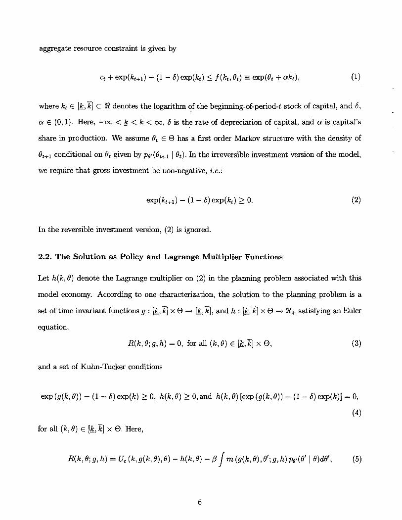
aggregate resource constraint is given by

ct + e x ~ ( k ~ + ~ ) - (1 - 6) exp(kt) I f (kt, ot) ex~(6 t + ak t )7 (1)

where kt E [k, x] C !It denotes the logarithm of the beginning-of-period-t stock of capital, and 6,

cu E (0,l) . Here, -cm < Ic < < cm, 6 is the rate of depreciation of capital, and cu is capital's

share in production. We assume Ot E O has a fist order Markov structure with the density of

8t+l conditional on 8, given by (8,+, I 8,). In the irreversible investment version of the model,

we require that gross investment be non-negative, i. e.:

In the reversible investment version, (2) is ignored.

2.2. The Solution as Policy and Lagrange Multiplier Functions

Let h(k, 8) denote the Lagrange multiplier on (2) in the planning problem associated with this

model economy. According to one characterization, the solution to the planning problem is a

set of time invariant functions g : [lc, x] x 8 -+ [lc, x], and h : [k, x] x 8 -+ !It+ satisfying an Euler

equation,

R(k, 8; g, h) = 0, for all (I;, 8) E [k, x] x 8, (3)

and a set of Kuhn-Tucker conditions

exp (g(k, 8)) - (1 - S) exp(k) 2 0, h(k, 6) 2 0, and h(k, 8) [ ~ X P (g(k, 8)) - (1 - 6) e x ~ ( k ) l = 0,

(4)

for all (k, 6) E [k, x] x 8 . Here,

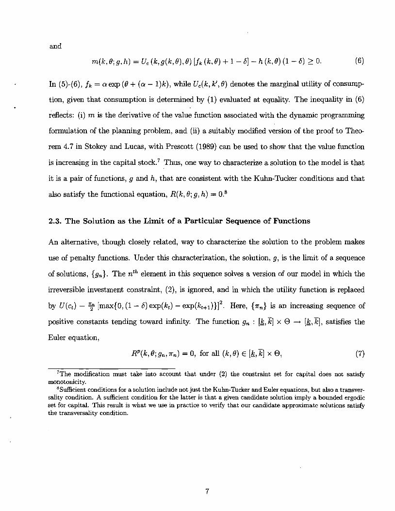
m(k, 8; g, h) = U, (k,g(k, 8), 8) [fk (k, 8) + 1 - 61 - h (k, 8) (1 - 6) > 0. (6 )

In (5)-(6), fk = cr exp (8 + (a - 1) k) , while U,(k, k', 8) denotes the marginal utility of consump

tion, given that consumption is determined by (1) evaluated at equality. The inequality in (6)

reflects: (i) m is the derivative of the value function associated with the dynamic programming

formulation of the planning problem, and (ii) a suitably modified version of the proof to Thee

rem 4.7 in Stokey and Lucas, with Prescott (1989) can be used to show that the value function

is increasing in the capital stock.' Thus, one way to characterize a solution to the model is that

it is a pair of functions, g and h, that are consistent with the Kuhn-Tucker conditions and that

also satisfy the functional equation, R(k, 8; g, h) = 0.8

2.3. T h e Solution as t h e Limit of a Particular Sequence of Functions

An alternative, though closely related, way to characterize the solution to the problem makes

use of penalty functions. Under this characterization, the solution, g, is the limit of a sequence

of solutions, {gn}. The nth element in this sequence solves a version of our model in which the

irreversible investment constraint, (2), is ignored, and in which the utility function is replaced

by U(c,) - f [max{O, (1 - 6) exp(kt) - exp(kt+l)}12. Here, {T,} is an increasing sequence of

positive constants tending toward infinity. The function g, : [k, 21 x Q -t [k, x], satisfies the

Euler equation,

RP(k, 8; gnr rn) = 0, for all (k, 8) E [&,El X 8,

7The modification must take into account that under (2) the constraint set for capital does not satisfy monotonicity.

MSufEcient conditions for a solution include not just the Kuhn-Tucker and Euler equations, but also a transver- sality condition. A sufficient condition for the latter is that a given candidate solution imply a bounded ergodic set for capital. This result is what we use in practice to verify that our candidate approximate solutions satisfy the transversality condition.

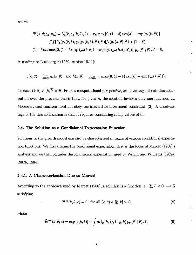
where

RP(k, 6; gn, r n ) = Uc(k, gn(k, e), 0) - r n ma{(), (1 - 6) exp(k) - exp(gn(k, 6)))

-PS{uc(gn(k,e),gn(gn(k,e),et),et)[fi,(gn(k,e),et) + (1 - 6)]

-(I - 6)rn ma[O, (1 - 6) exp (gn(k, 0)) - exp (gn (gn(k, e), e t ) ) ] )~e l (e t 1 e)de' = 0.

According to Luenberger (1969, section 10.11) :

g(k, 0) = lim gn(k, B), and h(k, 0) = lim rnmax{O, (1 - S)exp(k) - exp (gn(k, e))), n+oo n+oo

for each (k, 0) E [b, x] x O. From a computational perspective, an advantage of this character-

ization over the previous one is that, for given n, the solution involves only one function, 9,.

Moreover, that function need not obey the irreversible investment constraint, (2). A disadvan-

tage of the characterization is that it requires considering many values of n.

2.4. The Solution as a Conditional Expectation Function

Solutions to the growth model can also be characterized in terms of various conditional expecta-

tion functions. We first discuss the conditional expectation that is the focus of Marcet (1988)'s

analysis and we then consider the conditional expectation used by Wright and Williams (1982a,

1982b, 1984).

2.4.1. A Characterization Due to Marcet

According to the approach used by Marcet (1988), a solution is a function, e : [b, x] x O --+ 8

satisfying

RPa(k, e; e) = 0, for all (k, 8) E [b, k] x e, (8)

where

R P ~ ( ~ , e; e) = exp [e(k, e)] - 1 rn (g(k, e), 8'; g, h)pet(Bt I e)det,

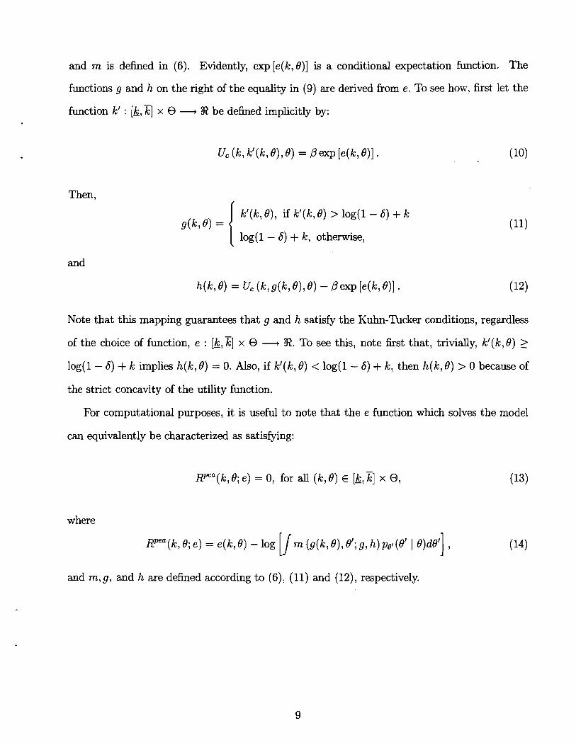
and m is defined in (6). Evidently, exp [e(k, 8)] is a conditional expectation function. The

functions g and h on the right of the equality in (9) are derived from e. To see how, first let, the

function k' : [lc, %] x @ - 8 be defined implicitly by:

Then,

( log(1 - 6) + k, otherwise,

Note that this mapping guarantees that g and h satisfy the Kuhn-Tucker conditions, regardless

of the choice of function, e : [b, x] x Q - 92. To see this, note first that, trivially, kl(k, 8) 2

log(1 - 6) + k implies h(k, 8) = 0. Also, if kl(k, 8) < log(1 - 6) + k, then h(k, 8) > 0 because of

the strict concavity of the utility function.

For computational purposes, it is useful to note that the e function which solves the model

can equivalently be characterized as satisfying:

RFa(k, 8; e) = 0, for all (k , 8) E [lc,x] x 8,

where

RPea(k, 8; e) = e(k, 8) - log [I m (g(k, 8), 8'; g, h)p~~(B1 I 8)d8'] ,

and m, g, and h are defined according to (6), (11) and (12), respectively.

2.4.2. A Characterization Due to Wright and Williams

Wright and Williams (1982a, 1982b, 1984) work with a slightly different conditional expectation

function. Their approach characterizes the solution as a function v : [b,z] x 8 ---, '8, satisfying

~ ~ ~ ( k ' , 8 ; v ) = 0, for all (kt,8) E [b,E] x e, (15)

where

and m is defined in (6). The functions g and h on the right of the equality in (16) are derived

from v as follows. First let the function kt : [&,El x 8 --, '8 be defined implicitly by:

Then, g and h are defined by (11) and

With the above operator from v to g and h, the Kuhn-Tucker conditions are not satisfied

for arbitrary v : [b,E] x El - 32. In particular, for a 7) function that is sufficiently increasing

in its first argument, kt (k, 0) < log(1 - 6) + k implies h(k, 8) < 0. Moreover, a sufficiently non-

monotone 71 function could imply a g that is a correspondence rather than a function. These may

not be problems in practice. First, it is easily verified that for 71 functions which are decreasing

in their first argument, the above operator does guarantee that the Kuhn-Tucker conditions are

satisfied and that g is a function. Second, concavity of the value function and the fact that m

is the derivative of the value function with respect to capital, implies that the exact 71 function

is decreasing in its first argument. Third, an operator useful in computing v, which maps the

space of functions 71 : [b,x] x O - '8 into itself, has the property of mapping the subspace

of v functions decreasing in kt into itself. For an arbitrary v this operator, P(v), is defined as

follows:

where g and h are obtained from v in the way described above.g Thus, as long as it begins with

a v function decreasing in kt, an algorithm that approximates v as the limit of a sequence of

functions generated by the P operator may never encounter v functions which imply g and h

that are not functions or are inconsistent with the Kuhn-Tucker conditions. Still, with other

model economies and other types of computational algorithms one clearly has to be on the alert

for these possibilities. We investigate them in the numerical analysis below.

2.4.3. Discussion

It is easily confirmed that the solutions to the four functional equations, R, Fa, Rpea, and

@", correspond to four equivalent characterizations of the solution to the model. Fkom a

computational perspective, however, they are quite different when (2) binds occasionally. A

computational strategy based on solving the functional equation, R = 0, requires finding two

functions, g and h, subject to the constraint that they satisfy the Kuhn-Tucker conditions. In

contrast, finding e to solve Rpea = 0, pa = 0, or v to solve ea = 0 involves having to findonly

one function. Moreover, strategies based on finding e need not impose any extra side conditions.

Finally, an argument presented above as well as numerical results reported below suggest that

in practice this may be true for 11 as well.

There are some additional differences between the characterizations based on e and v. First,

in our model economy the operator from e to g and h has a closed form expression and so

"0 establish that P(v) is decreasing in its first argument if v is, (19) indicates it is sufficient to verify that m is decreasing in its first argument whenever v is. Accordingly, consider a given v(k, 6) that is decreasing in k for (k, 6) E [&,XI x O. Fix 6 E O and consider first values of k interior to the set of points where the irreversibility constraint fails to bind. From the relation, Uc (k, g(k, 6), 6) = Bexp [v(g(k, 6), O)] , it is easily verified that U, (k,g(k, 6), 6) is increasing in k. But, m(k, 6; g, h) = Uc (k,g(k, 6), 6) [fk(k, 6) + 1 - 61. The result that m is decreasing in its first argument follows from the fact that Uc and f k are. Now suppose k lies in the interior of the set where the irreversibility constraint binds, so that g(k, 6) = log(1 - 6) + k. Then, substituting (18) into (6), we get m(k, 6;g, h) = Uc (k,g(k, 6), 6) fk(k, 6) + (1 - 6)Bexp [v(k, 6)] . That m is decreasing in k follows from the readily verified facts that Uc, v and f k are.

is trivial to implement computationaUy. In contrast, the analogous operator from v to g and

h requires solving a nonlinear equation, and so is computationally more burdensome. This

distinction per se does not seem important to us, since it reflects a special feature of our model

economy. In general the mapping from e to g and h also requires solving a nonlinear equation.

A potentially more significant difference is that the e and v functions being approximated differ

in their smoothness properties. Note:

v(kr,8) = log [Jm(kr,8';g,h)pol(8r( $)dor 1 , e(k78) = l o g [ J m ( g ( k 7 8 ) , ~ ' ; g , h ) p e ~ ( e r I8)der] =v(g(k,e),B).

The functions g and h are unlikely to be differentiable in k since they are expected to have a

kink at the value of capital where the irreversibility constraint starts to bind. We expect this

to result in a kink in e but not in v. That v is likely to be smooth in 8 follows from the fact

that for v to be differentiable in 8 requires only that pe1(er ( 8) be differentiable in 8. (Note,

if 8 is independent over time, then v is not even a function of 8, a great simplification from

a computational perspective.) To see why v may be differentiable in kt, note first that m is

expected to have a kink in k' at the value of capital where the irreversibility constraint starts to

bind (see the role of g in defining m in (6).) As long as that value varies non-trivially with the

value of 8, the effects of the lunk are expected to be smoothed over by the integration operator

that defines v.1° If v is smoothly differentiable and g is not, then e cannot be differentiable,

since e(k, 8) = a(g (k, 8), 8). The relative smoothness of v makes it an attractive function to

approximate numerically.

l0For example, suppose m(k, 8 ) = max(k, 0), for k, O E [k,z]. Then,

This integral is clearly differentiable in k, even though m(k, 0) is not.

2.5. Asset Prices

We are interested in the properties of the quantity allocations that solve the planning problem:

and also in the rates of return and prices in the underlying competitive decentralization. In

particular, we are interested in the consumption cost of end-of-period capital (i.e., Tobin's q)

and the rate of return on equity and risk free debt, Re and Rf. These are constructed:

It is easy to establish that 0 5 q(k, 8) 5 1. The result, q 5 1, follows from the non-negativity

of the Lagrange multiplier, h. The result, q 2 0, follows from (3), ( 5 ) , U, 2 0, and the non-

negativity of m in (6). The event in which the constraint binds corresponds to the event

q(k, 8) < 1. It is easily verified that in a competitive decentralization of this economy where

households own the capital stock and undertake investment, q is the price of end-of-period

capital in consumption units, Re is the rate of return on capital, and Rf is the rate of return

on risk free debt.ll The fourth power appears in (21) because we think of the time unit of the

model as being one quarter, while we express rates of return in annualized percentages.

3. Weighted Residual Solution Met hods

The computational algorithms we consider in this paper are special cases of the framework in

Reddy (1993)'s numerical analysis text, which corresponds closely to the framework presented

in Judd (1992a, 1992b). This framework is designed for problems in which one seeks a function,

say f : D -+ Q, which solves the functional equation, F(s; f ) = 0 for all s E D, where D is

"See Sargent (1980)jand Christian0 and Fisher (1995) for a more detailed analysis of Tobin's q in a general equilibrium environment like ours.

a compact set. This can be a diacult problem when, as in our case, there is a continuum of

elements in D. Then, finding a solution corresponds to a problem of solving a continuum of

equations (one for each s) in a continuum of unknowns (one f value for each s). Apart hom a

few special cases, in which F has a convenient structure, an exact solution to this problem is

computationally intractable.

Instead, we select a function, A, parameterized by a finite set of coefficients, a, and choose

values for a, a*, to make F(s; A) 'small'. Weighted-residual methods compute a* as the solution

to what Reddy (1993, p. 580) refers to as the weighted-residual form:

where i ranges hom unity to a number which equals the dimension of a. Expression (22) corre-

sponds to a number of equations equal to the number of unknowns in a. The choice of weighting

functions in (22) operationalizes the notion of 'small'. For example, if for some i, wi = 1 for all

s, then F(s; A ) small means, among other things, that the average of F(s; Ta), over all possible

s, is zero. If for some i, w' is a Dirac delta function isolating some particular point s, then

F(s ; L) small means it is precisely zero at that point, and so on.

To apply the weighted-residual method, one has to select a family of approximating functions,

L, a set of weighting functions, wi(s) , and strategies for evaluating the integral (22) and any

integrals that may go into defining F. The procedures we consider make different choices on

these three dimensions. Two general types of fl, functions include spectral and finite element

functions. In the former, each component of a influences fa, over the whole range of s while in

the latter, each component of a has influence over only a limited range of s's. We consider three

types of weighting functions. In one, the wi(s)'s are related to the basis functions generating A, in which case the algorithm is an example of the Galerkzn method. In another, a is chosen so

that F is zero at a number of values of s equal to the number of unknown elements in a. In this

case, the wi(s)'s are Dirac delta functions, and the algorithm is an example of the collocation

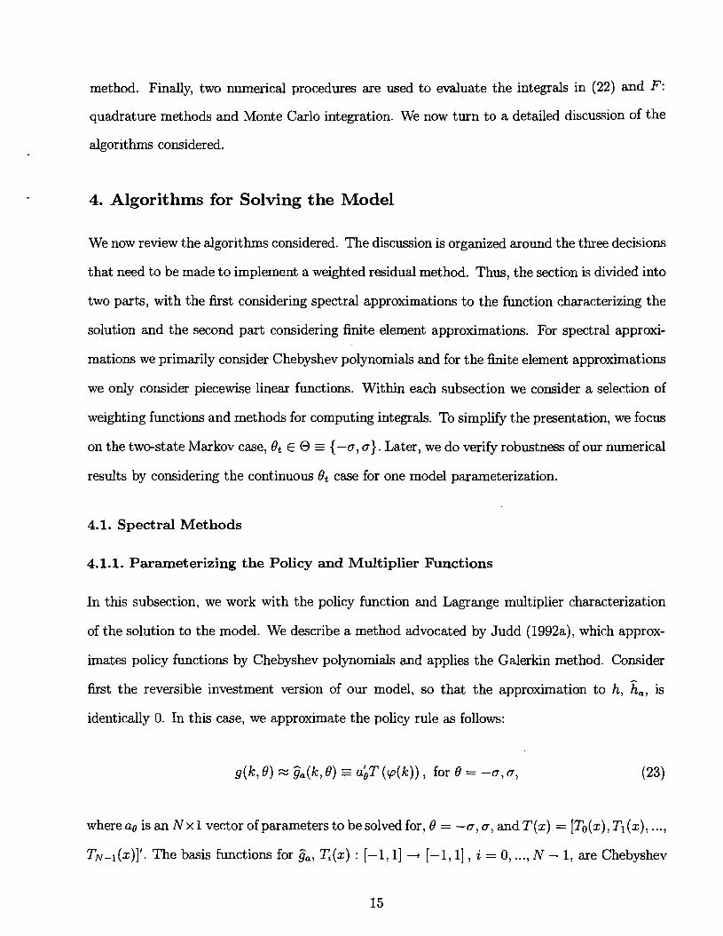
method. Finally, two numerical procedures are used to evaluate the integrals in (22) and F:

quadrature methods and Monte Carlo integration. We now turn to a detailed discussion of the

algorit hrns considered.

4. Algorithms for Solving the Model

We now review the algorithms considered. The discussion is organized around the three decisions

that need to be made to implement a weighted residual method. Thus, the section is divided into

two parts, with the first considering spectral approximations to the function characterizing the

solution and the second part considering finite element approximations. For spectral approxi-

mations we primarily consider Chebyshev polynomials and for the finite element approximations

we only consider piecewise linear functions. Within each subsection we consider a selection of

weighting functions and methods for computing integrals. To simplify the presentation, we focus

on the twestate Markov case, Ot E O - (-0, o). Later, we do verify robustness of our numerical

results by considering the continuous 9t case for one model parameterization.

4.1. Spectral Methods

4.1.1. Parameterizing the Policy and Multiplier Functions

In t h s subsection, we work with the policy function and Lagrange multiplier characterization

of the solution to the model. We describe a method advocated by Judd (1992a), which approx-

imates policy functions by Chebyshev polynomials and applies the Galerkin method. Consider

first the reversible investment version of our model, so that the approximation to h, Za, is

identically 0. In this case, we approximate the policy rule as follows:

g(k, 0) Ga(k, 0) E abT ( ~ ( k ) ) , for 0 = -0, o, (23)

where a0 is an N x 1 vector of parameters to be solved for, 0 = -0, o, and T (x) = [To(x), TI (x), . . . ,

TN-i (x)]'. The basis functions for Ga, Z(x) : [- 1,1] -t [- 1,1] , i = 0, .. . , N - 1, are Chebyshev

polynomials.12 Also,

Let a = [a: aL,]' denote the 2N x 1 dimensional vector of parameters for 3,.

The 2N weighting functions, wi (k, 8), are constructed from the basis functions as follows:

for i = 1, . . . ,2N. It is readily verified from (23) that one of dGa(k, a)/dai and dGa(kl -a) Idai is

zero and the other is a Chebyshev polynomial, for each i.

In the irreversible investment version of the model, we must parameterize the policy and

Lagrange multiplier functions so that they respect the Kuhn-Tucker conditions, (4). We impose

(and subsequently verify) that the irreversible investment constraint never binds for 8 = a .

Thus, we restrict the space of approximating functions for g(k, 8) as follows:

g(k, -a) x &(k, -a) - max{ija(k),log(l - 6) + k}, for all k f [k,x]. (27)

Also, /

We choose functional forms for $(k, a ) , &(k), and &(k) as follows:

Here, T is the N x 1 column vector of Chebyshev polynomials defined after (23), and a,, a_,,

b are N x 1 column vectors of parameters. All elements of a, are permitted to be non-zero,

12The Chebyshev polynomials are defined as follows: To(x) 1, Tl ( x ) = X , and T ~ ( x ) = 2~Ti-1 ( x ) - Ti -2(~) , for i > 2.

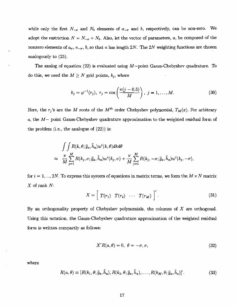
while only the first N-, and Nb elements of a_, and b, respectively, can be non-zero. We

adopt the restriction N = N-, + Nb. Also, let the vector of parameters, a, be composed of the

nonzero elements of a,, a_,, b, so that a has length 2N. The 2N weighting functions are chosen

analogously to (25).

The analog of equation (22) is evaluated using M-point Gauss-Chebyshev quadrature. To

do this, we need the M 1 N grid points, kj, where

1 r(j - 0.5) kj = cp- (rj), rj = cos ( ) , j = l , - - - , ~

Here, the rj's are the M roots of the Mth order Chebyshev polynomial, TM(x). For arbitrary

a, the M- point Gauss-Chebyshev quadrature approximation to the weighted residual form of

the problem (i.e., the analogue of (22)) is:

for i = 1, ..., 2N. To express this system of equations in matrix terms, we form the M x N matrix

X of rank N:

By an orthogonality property of Chebyshev polynomials, the columns of X are orthogonal.

Using this notation, the Gauss-Chebyshev quadrature approximation of the weighted residual

form is written compactly as follows:

where

Expression (32) represents a nonlinear system of 2N equations in the 2N unknowns, a, which can

be solved using widely available software.13 Below, we refer to this method as Spectral-Galerkin.

For later purposes it is convenient to note that if M = N, then X is square and invertible, A

so the method reduces to setting R(kj,Q;Zja,ha) = 0 for j = 1, ..., M and for 0 = -a ,a . In this

case, Spectral-Galerkin reduces to a collocation method.

4.1.2. Parameterizing the Conditional Expectation

We now discuss methods based on approximati~lg conditional expectations. We distinguish be-

tween the type of conditional expectation being approximated and the method used to compute

the approximation. We consider two types of conditional expectations, the one that is the focus

of Marcet (1988)'s analysis (see e in (9) or (14)) and the one that is the focus in Wright and

Williams (1982a, 1982b, 1984) (see v in (16)). We consider two ways of approximating the con-

ditional expectation, one based on the nonlinear regression methods advocated by Marcet (1988)

and another that is closely related to the methods advocated by Judd (1992a) for approximating

policy rules. To simplify the discussion, we focus on methods that approximate the e function

and we indicate briefly how the methods must be adjusted to obtain an approximation to v.

For PEAS which approximate e,

Here, %(k, 0) is a function with a finite set of parameters, a. In the reversible investment version A

of our model economy, ha - 0 and the relation linking the policy function, Ga, to e , can be

expressed analytically:

$(k, 0) = log {exp(Q + at) + (1 - 6 ) exp(k) - U;' [P exp ($(k, e))]) , (35)

where U,-'[-] is the level of consumption implied by a given value for U,. In the irreversible

l w e apply the versions of the Newton-Raphson method implemented in the GAUSS routine, NLSYS.

18

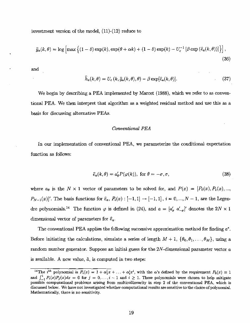
investment version of the model, (11)-(12) reduce to

&(k, 8) = log [max {(I - 6) exp(k), exp(8 + ak) + (1 - 6) exp(k) - U;' [Dexp ($(k, g))])] ,

(36)

and

ha(k,8) = U c (k,9a(k,e),Q) - Dex~[e^,(k,9)]- (37)

We begin by describing a PEA implemented by Marcet (1988), which we refer to as conven-

tional PEA. We then interpret that algorithm as a weighted residual method and use this as a

basis for discussing alternative PEAS.

Conventional PEA

In our implementation of conventional PEA, we parameterize the conditional expectation

function as follows:

Za(k, 9) = aLP(p(k)), for 8 = -a, a, (38)

where a0 is the N x 1 vector of parameters to be solved for, and P(x) = [Po(x), Pl (x) , ...,

PN-l(~)] ' . The basis functions for e^,, P,(x) : [-I, I.] -t [-I, 11 , i = 0, ..., N - 1, are the Legen-

dre polynomial^.'^ The function p is defined in (24), and a = [a; ai,]' denotes the 2N x 1

dimensional vector of parameters for Za.

The conventional PEA applies the following successive approximation method for finding a*.

Before initiating the calculations, simulate a series of length M + 1, {O0,81,. . . , O M ) , using a

random number generator. Suppose an initial guess for the 2N-dimensional parameter vector a

is available. A new value, 6, is computed in two steps:

14The i th polynomial is Pi(x) = 1 + crfx + . . . + crfxi, with the a's defined by the requirement Po(x) -= 1 and J:~ Pi(x)Pj(x)dx = 0 for j = 0,. . . , i - 1 and i 2 1. These polynomials were chosen to help mitigate possible computational problems arising from multicollinearity in step 2 of the conventional PEA, which is discussed below. We have not investigated whether computational results are sensitive to the choice of polynomial. Mathematically, there is no sensitivity.

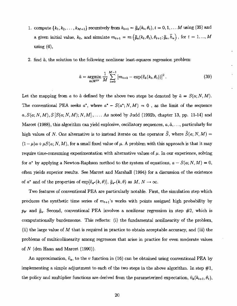
1. compute {kl,'k2, . . . , kM+l} recursively fiom kt+l = &(kt, Bt), t = 0,1, . . . M using (35) and A

a given initial value, ko, and simulate mt+l = rn (&(kt, Bt), Bt+1; $, ha) : for t = 1, ... , M

using (61,

2. find 6, the solution to the following nonlinear least-squares regression problem:

Let the mapping fiom a to Ti defined by the above two steps be denoted by Ti = S(a; N, M).

The conventional PEA seeks a*, where a* - S(a*; N, M) = 0 , as the limit of the sequence

a, S(a; N, M), S [S(a; N, M); N, MI, . . . . As noted by Judd (1992b, chapter 13, pp. 11-14) and

Marcet (1988), this algorithm can yield explosive, oscillatory sequences, a, Ti, . . ., particularly for

high values of N. One alternative is to instead iterate on the operator 3, where S(a; N, M) =

(1 - p)a+pS(a; N, M), for a small fixed value of p. A problem with this approach is that it may

require time-consuming experimentation with alternative values of p. In our experience, solving

for a* by applying a Newton-Raphson method to the system of equations, a - S(a; N, M) = 0,

often yields superior results. See Marcet and Marshall (1994) for a discussion of the existence

of a* and of the properties of exp[e^,.(k, Q)], &(k, 8) as M, N -+ oo.

Two features of conventional PEA are particularly notable. First, the simulation step whch

produces the synthetic time series of rnt+1's works with points assigned high probability by

pol and &. Second, conventional PEA involves a nonlinear regression in step #2, which is

computationally burdensome. This reflects: (i) the fundamental nonlinearity of the problem,

(ii) the large value of M that is required in practice to obtain acceptable accuracy, and (iii) the

problems of multicollinearity among regressors that arise in practice for even moderate values

of N (den Haan and Marcet (1990)).

An approximation, Ga, to the v function in (16) can be obtained using conventional PEA by

implementing a simple adjustment to each of the two steps in the above algorithm. In step #1,

the policy and multiplier functions are derived fiom the parameterized expectation, Ca(kt+l, Qt),

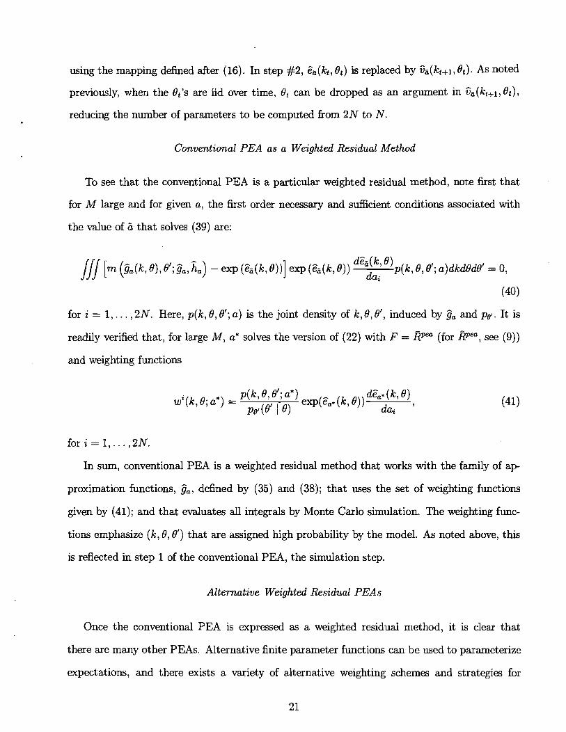
using the mapping defined after (16). In step #2, &(h, Ot) is replaced by Ga(kt+l, 8,). As noted

previously, when the Ot1s are iid over time, Ot can be dropped as an argument in Ca(kt+l, Ot),

reducing the number of parameters to be computed from 2N to N.

Conventional PEA as a Weighted Residual Method

To see that the conventional PEA is a particular weighted residual method, note first that

for M large and for given a, the f i s t order necessary and sufficient conditions associated with

the value of ?I that solves (39) are:

dZ6(k, 8) JJJ [m (&(kl 8), 8';$, ha) - ex^ ( h ( k l 8))] exp (w, 8)) dai p(k, 8,8'; a)dkdOdO1 = 0,

(40)

for i = 1, . . . ,2N. Here, p(k, 8,01; a) is the joint density of k, 8, Of, induced by Ga and Pel. It is

readily verified that, for large M, a* solves the version of (22) with F = RP" (for ~ p ~ ~ , see (9))

and weighting functions

p(k, 8,01; a*) wi(k, 8; a*) = exp(e^,* (k18)) dZa* (k, 8)

pel(Of I 0) dai 1

f o r i = 1 , . . . , 2N.

In sum, conventional PEA is a weighted residual method that works with the family of a p

proximation functions, Gal defined by (35) and (38); that uses the set of weighting functions

given by (41); and that evaluates all integrals by Monte Carlo simulation. The weighting func-

tions emphasize (k, 8,01) that are assigned high probability by the model. As noted above, t h s

is reflected in step 1 of the conventional PEA, the simulation step.

Alternative Weighted Residual PEAs

Once the conventional PEA is expressed as a weighted residual method, it is clear that

there are many other PEAs. Alternative finite parameter functions can be used to parameterize

expectations, and there exists a variety of alternative weighting schemes and strategies for

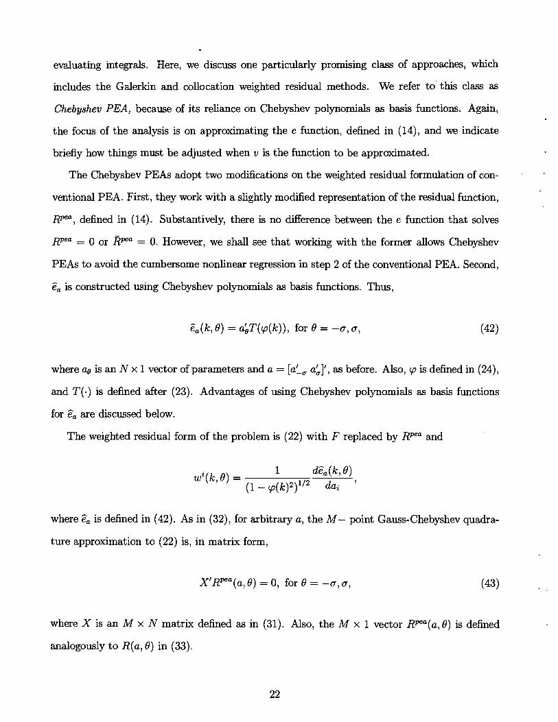
evaluating integrals. Here, we discuss one particularly promising class of approaches, which

includes the Galerkin and collocation weighted residual methods. We refer to this class as

Chebyshev PEA, because of its reliance on Chebyshev polynomials as basis functions. Again,

the focus of the analysis is on approximating the e function, defined in (14), and we indicate

briefly how things must be adjusted when v is the function to be approximated.

The Chebyshev PEAS adopt two modifications on the weighted residual formulation of con- .

ventional PEA. First, they work with a slightly modified representation of the residual function,

Rpa, defined in (14). Substantively, there is no difference between the e function that solves

RPe" = 0 or Wa = 0. However, we shall see that working with the former allows Chebyshev

PEAS to avoid the cumbersome nonlinear regression in step 2 of the conventional PEA. Second,

e^, is constructed using Chebyshev polynomials as basis functions. Thus,

G(k, 8) = aLT(cp(k)), for 8 = -0, o ,

where a0 is an N x 1 vector of parameters and a = [a'_, a;]', as before. Also, cp is defined in (24),

and T(-) is defined after (23). Advantages of using Chebyshev polynomials as basis functions

for e , are discussed below.

The weighted residual form of the problem is (22) with F replaced by Rpa and

where e^, is defined in (42). As in (32), for arbitrary a, the M- point Gauss-Chebyshev quadra-

ture approximation to (22) is, in matrix form,

X'Rpa(a, 8) = 0, for 8 = -(T, o, (43)

where X is an M x N matrix defined as in (31). Also, the M x 1 vector Rpa(a,8) is defined

analogously to R(a, 8) in (33).

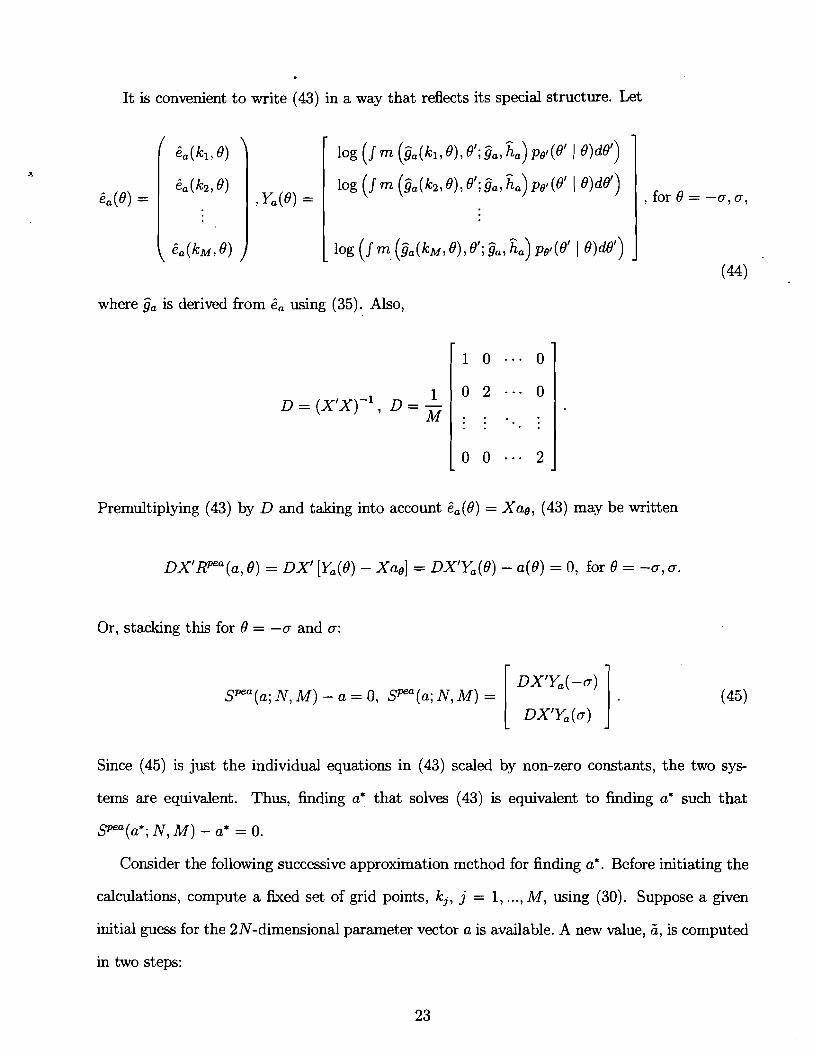
It is convenient to write (43) in a way that reflects its special structure. Let

where ija is derived from 6, using (35). Also,

Premultiplying (43) by D and taking into account Ga(8) = Xuo, (43) may be written

DX'RPa(a, 8 ) = DX' [Ya(8) - Xue] = DX1Ya(B) - a(0) = 0, for 8 = -a, a.

Or, stacking this for 8 = -a and a:

Since (45) is just the individual equations in (43) scaled by non-zero constants, the two sys-

tems are equivalent. Thus, finding a* that solves (43) is equivalent to finding a* such that

P a ( a * ; N, M ) - a* = 0.

Consider the following successive approximation method for finding a*. Before initiating the

calculations, compute a fixed set of grid points, k,, j = 1 , ..., M, using (30). Suppose a given

initial guess for the 2N-dimensional parameter vector a is available. A new value, 6, is computed

in two steps:

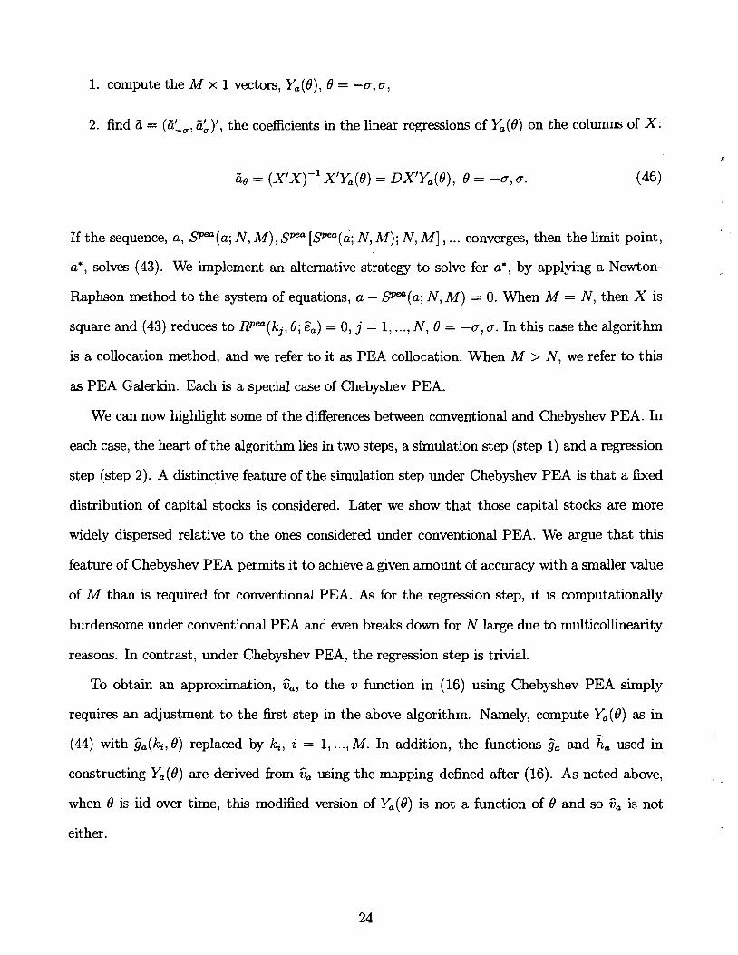
1. compute the M x 1 vectors, Ya(8), 8 = -a,a,

2. find 5 = (X, , Zk)', the coefficients in the linear regressions of Ya(8) on the columns of X :

If the sequence, a, Spea (a; N, M) , SPea [Spea(a; N, M) ; N, MI , .. . converges, then the limit point,

a*, solves (43). We implement an alternative strategy to solve for a*, by applying a Newton-

Raphson method to the system of equations, a - P a ( a ; N, M) = 0. When M = N, then X is

square and (43) reduces to Rpea(kj, 8; Za) = 0, j = 1, ..., N, 8 = -a, a . In this case the algorithm

is a collocation method, and we refer to it as PEA collocation. When M > N, we refer to this

as PEA Galerkin. Each is a special case of Chebyshev PEA.

We can now highlight some of the differences between conventional and Chebyshev PEA. In

each case, the heart of the algorithm lies in two steps, a simulation step (step 1) and a regression

step (step 2). A distinctive feature of the simulation step under Chebyshev PEA is that a fixed

distribution of capital stocks is considered. Later we show that those capital stocks are more

widely dispersed relative to the ones considered under conventional PEA. We argue that this

feature of Chebyshev PEA permits it to achieve a given amount of accuracy with a smaller value

of M than is required for conventional PEA. As for the regression step, it is computationally

burdensome under conventional PEA and even breaks down for N large due to multicollinearity

reasons. In contrast, under Chebyshev PEA, the regression step is trivial.

To obtain an approximation, Ga, to the 71 function in (16) using Chebyshev PEA simply

requires an adjustment to the fist step in the above algorithm. Namely, compute Ya(8) as in

(44) with ea(ki, 8) replaced by ki, i = 1, . . . , M. In addition, the functions $ and za used in

constructing Ya (8) are derived from 13, using the mapping defined after (16). As noted above,

when 8 is iid over time, this modified version of Ya(8) is not a function of 8 and so 13, is not

either.

4.1.3. The Role of Chebyshev Polynomials in Chebyshev PEA

We now discuss some of the advantages of using Chebyshev polynomials in Chebyshev PEA.

First, the orthogonality property of the columns of X defined after (43) reflects that we construct

the grid of kj's based on the zeros of a Chebyshev polynomial. This is why the linear regression

step in (46) is trivial. For example, we have applied the algorithm without difficulty with N as

high as 100. In contrast, we had difficulty executing the regression step in conventional PEA

(see (39)) for N larger than 5 because of multicollinearity problems.

Second, the Chebyshev interpolation theorem (see Judd (1992a, 1992b)) provides some mo-

tivation for selecting the grid of capital stocks based on the roots of a Chebyshev polynomial,

at least for PEA collocation. There is some hope that one can establish

when M = N. To see this, note first that the v which solves the model is the fixed point, v = Po,

of a particular operator, P , defined in (19). The PEA collocation method for computing Gi can

be characterized as finding values for the 2N parameters, a, that solve:

Ga(ki,8) = P(Ga)(ki,O), for i = 1, ..., N, and 0 = -a ,a ,

where the ki's are chosen according to (30) with M = N.

Consider vb(ki, 0) = zLil bi(8)T(v(ki)), the N- lth order Chepyshev polynomial interpolant

of 7). That is the 2N parameters, b, are uniquely defined by:

vb(ki,O) = v(ki,O), for i = 1, ..., N, and 8 = - 0 , ~ .

By the Chebyshev approximation theorem, if v is at least differentiable once, then vb has the

following convergence property

It turns out that, for large enough N, Ga is similar to vb, and so can perhaps be expected to

share the convergence property attributed to vb by the Chebyshev approximation theorem. To

see this, note that, for ~b = vb - v,

where PN(g) = P(g - E ~ ) . Notice that the parameters, b, of vb and the parameters, a, of Ga solve

essentially the same set of equations as N --, oo, so that, we can expect,

The desired result, (47), would follow from the triangle inequality, 116, - 71 1 1 I IIGa - vb 1 1 + ( 1 vb - v 1 1 , and (49), if (51) were established formally. This has not yet been done. Note that in

this argument we only used the idea that the function being approximated is the fixed point of

an operator, and so it should be possible to use it to also analyze the convergence properties of

other approximations, such as Ga under Spectral-Galerkin with M = N.

4.2. Finite Element Methods

We consider the simplest class of finite element functions, those that are piecewise linear and

continuous in Ic for each fixed 8.'-e study a collocation (FEM collocation) and Galerkin

(FEM Galerkin) procedure for computing the parameters of this function. For FEM collocation, - A

a method advocated by Bizer and Judd (1989), Coleman (1988), Coleman, Gilles, and Labadie

-

15Reddy (1993) describes systematic procedures for expanding the space of finite element functions to include more than one dimension, and piecewise polynomials of order higher than one.

(1992) and Danthine and Donaldson (1981), we work with the characterization of the solution in

terms of policy and multiplier functions. For FEM Galerkin, a method advocated by McGrattan

(1993), we work with the penalty function formulation of the planning problem.

We find it convenient to begin with a description of the policy and multiplier functions

relevant to the reversible investment version of the model, so that La = 0. The 2N x 1 vector of

parameters of ijal a = (a'_,, a:)', with ae = (al,e, ..., aN,e)', specify the values of k' = ija(k, 0) at -

each point on a grid of N capital stocks, kj, j = 1, ..., N, for 0 = -a,u. Here, k1 2 k-, kN 5 k

and kj < kj+l1 j = 1, ..., N - 1. We specify that the capital stock grid is composed of equispaced

points. Thus, k' corresponding to (ki, 0) is ai,e = Ca(kil O), for 0 = -0, a, i = 1,2,. . . , N. Policy

decisions between points (ki, 0) are defined by linearly interpolating the decisions at the two

nearest such points. Formally,

ija(k, 0) E aLL(k),- for 0 = -a, a .

Here, L(k) = [Ll (k), Lz(k), ..., LN (k)]' is composed of the basis functions for ija:

k-ki-1 ki-l 5 k 5 ki

ki 5 k 5 ki+l

elsewhere,

fo r i=2 ,3 , ... N - 1 , and

( 0, elsewhere, I O1 elsewhere.

In the following two subsections, we describe a collocation and a Galerkin procedure for

devising a set of 2N weighting functions which can be used in conjunction with equation (22)

to find a.

4.2.1. Collocation

Consider first the reversible investment version of the model. FEM-collocation selects values for

a so that

R(ki, 8; ca , 0) = 0, (53)

for i = 1,2, . . . , N and 0 = -a, a . This is (22), with the weighting functions constructed using

suitably chosen Dirac-delta functions. Equation (53) is a nonlinear system of 2N equations in

the 2N unknowns, a. In practice, a method of successive approximation is used to solve (53).

In particular, suppose a given initial guess for the parameter vector a is available. A new value,

Zi, is computed as follows. For each element of the capital grid ki and for 0 = -a, a , find the

Zii,@ that solves

Denote the mapping from a to Zi by Zi = SF(a; N). The method seeks a*, where a* - SF(a*; N) =

0, as the limit of the sequence a, SF(a; N), S [sF(a; N); N] , . . . .

Now consider the irreversible investment version of the model. We work with policy and

multiplier functions parameterized according to (26)-(28). We choose piecewise linear functions

to form ea(k, o), B(k) , and Ka(k) and select the N-point capital stock grid as in the reversible

investment case. The objective is to solve for the coefficients associated with this grid: a;,@,

i = 1,2, . . . , N, 0 E O, as before. In addition, we seek bi, i = 1,2 , . . . , N, where bi corresponds

to ha(ki). Stack the undetermined coefficients in the vector a :

We modify the successive approximation algorithm described above as follows. The main step

of that algorithm, (54) for 0 = a, is replaced by

Uc(ki, a*,,, a) = Pipel (0 I B)Uc(ai,o , Ga(ai,o, 0) 0) [fk(ai,o 7 0) + 1 - 61

Equation (54) for'@ = -a is replaced by:

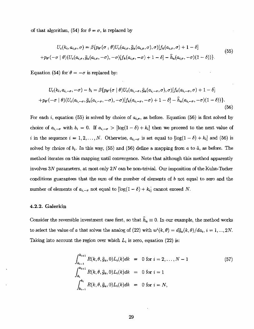
For each i, equation (55) is solved by choice of a;,,, as before. Equation (56) is first solved by

choice of a,,-, with b, = 0. If air-, > [log(l - 6) + ki] then we proceed to the next value of

i in the sequence i = 1,2, . . . , N. Otherwise, a,,-, is set equal to [log(l - 6) + ki] and (56) is

solved by choice of bi. In this way, (55) and (56) define a mapping from a to 6, as before. The

method iterates on this mapping until convergence. Note that although this method apparently

involves 3N parameters, at most only 2N can be non-trivial. Our imposition of the Kuhn-Tucker

conditions guarantees that the sum of the number of elements of b not equal to zero and the

number of elements of a,,-, not equal to [log(l - 6) + ki] cannot exceed N.

4.2.2. Galerkin

Consider the reversible investment case first, so that ^ha - 0. In our example, the method works

to select the value of a that solves the analog of (22) with wi (k, 8) = dGa(k, 0)/dai, i = 1, ..., 2N.

Taking into account the region over which Li is zero, equation (22) is:

ki+l

/ R ( ~ , B , & , ~ ) ~ ~ ( k ) d k = o for i = 2,. . . , N - I ki-1

ki+l 6, R(k, 8, Gay O)Li(k)dk = O for i = I

k; / R(k, 0, Ga, O)Li(k)dk = 0 for i = N, ki-1

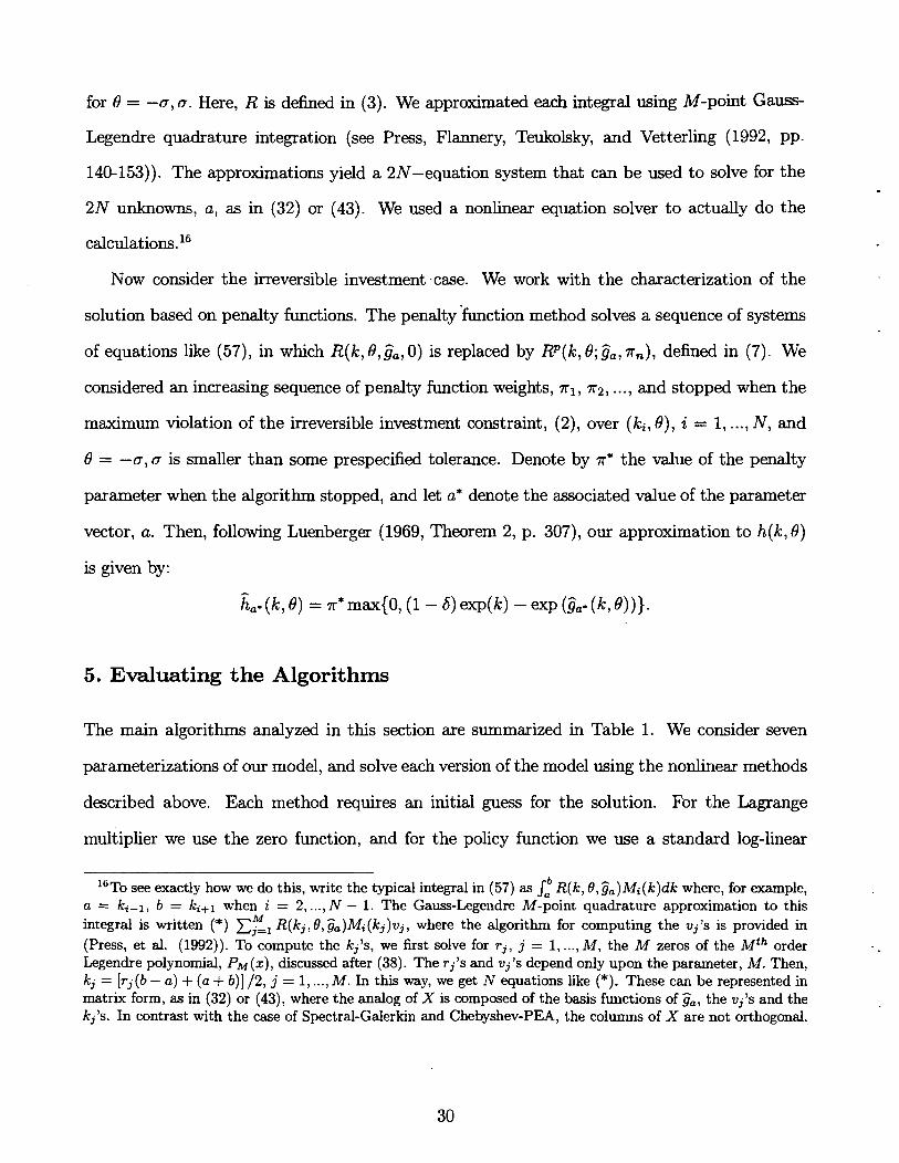
for 0 = -0, a. Here, R is defined in (3). We approximated each integral using M-point Gauss-

Legendre quadrature integration (see Press, Flannery, Teukolsky, and Vetterling (1992, pp.

140-153)). The approximations yield a 2N-equation system that can be used to solve for the

2N unknowns, a, as in (32) or (43). We used a nonlinear equation solver to actually do the

calculations. I"

Now consider the irreversible investment -case. We work with the characterization of the

solution based on penalty functions. The penalty 'function method solves a sequence of systems

of equations like (57), in which R(k, 0, ija, 0) is replaced by RP(k, 0; ija, T,), defined in (7). We

considered an increasing sequence of penalty function weights, TI, T ~ , . . ., and stopped when the

maximum violation of the irreversible investment constraint, (2), over (ki, a), i = 1, . .. , N, and

0 = -0, o is smaller than some prespecified tolerance. Denote by T* the value of the penalty

parameter when the algorithm stopped, and let a* denote the associated value of the parameter

vector, a. Then, following Luenberger (1969, Theorem 2, p. 307), our approximation to h(k, 0)

is given by:

5. Evaluating the Algorithms

The main algorithms analyzed in this section are summarized in Table 1. We consider seven

parameterizations of our model, and solve each version of the model using the nonlinear methods

described above. Each method requires an initial guess for the solution. For the Lagrange

multiplier we use the zero function, and for the policy function we use a standard log-linear

l U ~ o see exactly how we do this, write the typical integral in (57) as J: R(k, 8, ca)Mi(k)dk where, for example, a = ki-l, b = ki+l when i = 2, ..., N - 1. The Gauss-Legendre M-point quadrature approximation to this integral is unitten (*) xgl R(kj,8,ca)Mi(kj)vj, where the algorithm for computing the vj7s is provided in (Press, et al. (1992)). To compute the kj's, we first solve for r j , j = 1, ..., M, the M zeros of the M~~ order Legendre polynomial, PM (x), discussed after (38). The rj's and vj's depend only upon the parameter, M. Then, kj = [rj(b - a) + (a + b)] 12, j = 1, ..., M. In this way, we get N equations like (*). These can be represented in matrix form, as in (32) or (43), where the analog of X is composed of the basis functions of Fa, the vj's and the kj's. In contrast with the case of Spectral-Galerkin and Chebyshev-PEA, the columns of X are not orthogonal.

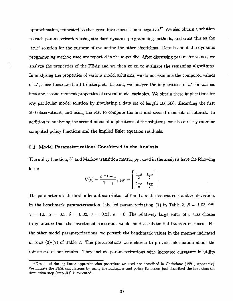
approximation, truncated so that gross investment is non-negative.17 We also obtain a solution

to each parameterization using standard dynamic programming methods, and treat this as the

'true' solution for the purpose of evaluating the other algorithms. Details about the dynamic

programming method used are reported in the appendix. After discussing parameter values, we

analyze the properties of the PEAS and we then go on to evaluate the remaining algorithms.

In analyzing the properties of various model solutions, we do not examine the computed values

of a*, since these are hard to interpret. Instead, we analyze the implications of a* for various

first and second moment properties of several model variables. We obtain these implications for

any particular model solution by simulating a data set of length 100,500, discarding the first

500 observations, and using the rest to compute the first and second moments of interest. In

addition to analyzing the second moment implications of the solutions, we also directly examine

computed policy functions and the implied Euler equation residuals.

5.1. Model Pararneterizations Considered in t h e Analysis

The utility function, U, and Markov transition matrix, pel, used in the analysis have the following

form:

The parameter p is the first order autocorrelation of 0 and o is the associated standard deviation.

In the benchmark parameterization, labelled parameterization (1) in Table 2, P = 1.03-0.25,

y = 1.0, a = 0.3, 6 = 0.02, a = 0.23, p = 0. The relatively large value of o was chosen

to guarantee that the investment constraint would bind a substantial fraction of times. For

the other model parameterizations, we perturb the benchmark values in the manner indicated

in rows (2)-(7) of Table 2. The perturbations were chosen to provide information about the

robustness of our results. They include parameterizations with increased curvature in utility

17Details of the log-linear approximation procedure we used are described in Christian0 (1991, Appendix). We initiate the PEA calculations by using the multiplier and policy functions just described the first time the simulation step (step #1) is executed.

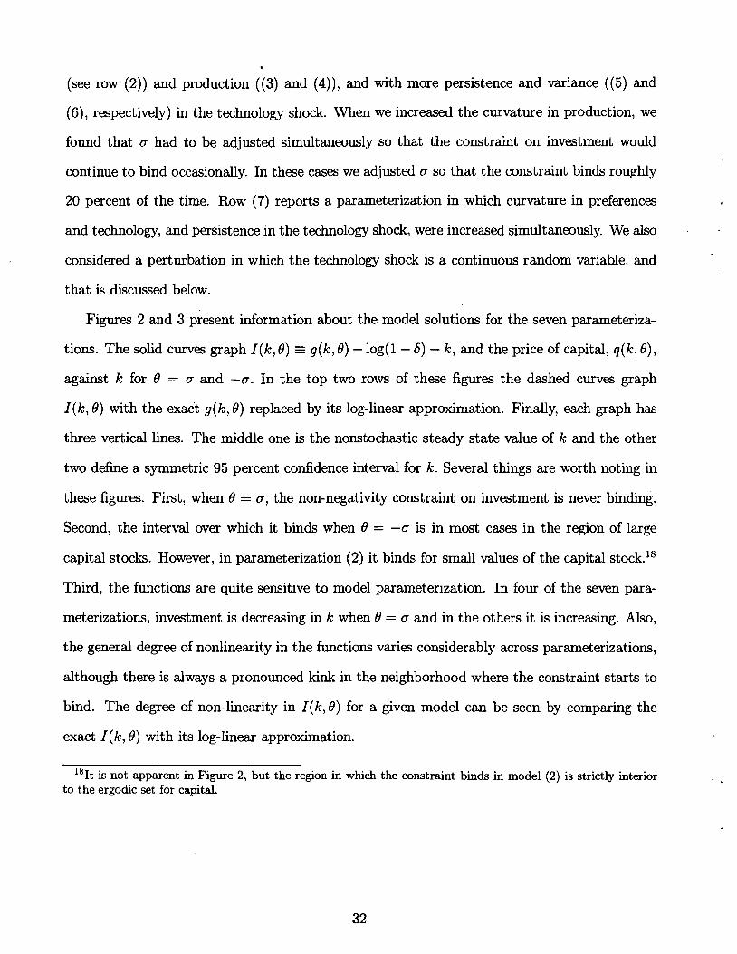
(see row (2)) and production ((3) and (4)), and with more persistence and variance ((5) and

(6 ) , respectively) in the technology shock. When we increased the curvature in production, we

found that a had to be adjusted simultaneously so that the constraint on investment would

continue to bind occasionally. In these cases we adjusted a so that the constraint binds roughly

20 percent of the time. Row (7) reports a parameterization in which curvature in preferences

and technology, and persistence in the technology shock, were increased simultaneously. We also .

considered a perturbation in which the technology shock is a continuous random variahle, and

that is discussed below.

Figures 2 and 3 present information about the model solutions for the seven parameteriza-

t ion~. The solid curves graph I(k, 0) = g(k, 0) - log(1- 6) - k, and the price of capital, q(k, O),

against k for 0 = a and -a. In the top two rows of these figures the dashed curves graph

I(k, 0) with the exact g(k, 0) replaced by its log-linear approximation. Finally, each graph has

three vertical lines. The middle one is the nonstochastic steady state value of k and the other

two define a symmetric 95 percent confidence interval for k. Several things are worth noting in

these figures. First, when 0 = a, the non-negativity constraint on investment is never binding.

Second, the interval over which it binds when 0 = -a is in most cases in the region of large

capital stocks. However, in parameterization (2) it binds for small values of the capital stock.18

Third, the functions are quite sensitive to model parameterization. In four of the seven para-

meterization~, investment is decreasing in k when 6 = a and in the others it is increasing. Also,

the general degree of nonlinearity in the functions varies considerably across parameterizations,

although there is always a pronounced kink in the neighborhood where the constraint starts to

bind. The degree of non-linearity in I(k, 0) for a given model can be seen by comparing the

exact I (k, 0) with its log-linear approximation.

l8It is not apparent in Figure 2, but the region in which the constraint binds in model (2) is strictly interior to the ergodic set for capital.

5.2. The PEAS

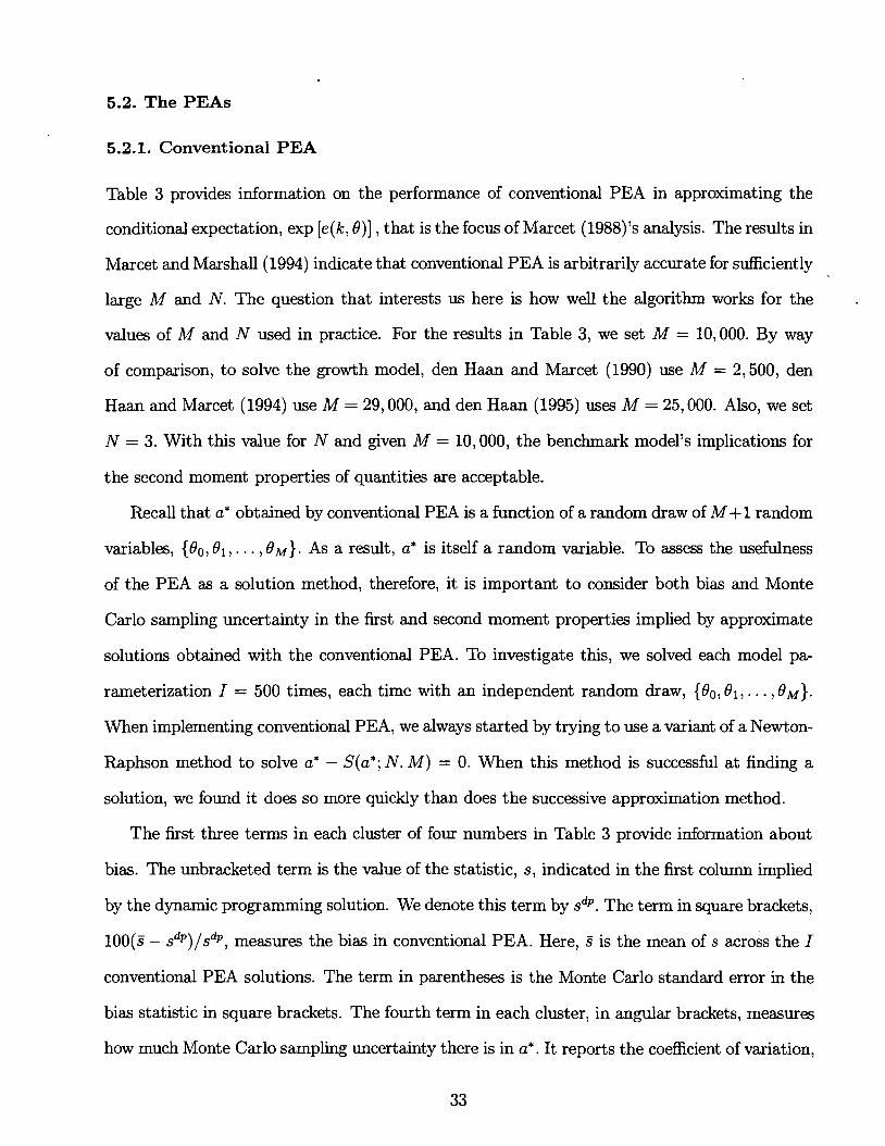
5.2.1. Conventional PEA

Table 3 provides information on the performance of conventional PEA in approximating the

conditional expectation, exp [e (k , O)] , that is the focus of Marcet (1988)'s analysis. The results in

Marcet and Marshall (1994) indicate that conventional PEA is arbitrarily accurate for sufficiently

large M and N. The question that interests us here is how well the algorithm works for the

values of M and N used in practice. For the results in Table 3, we set M = 10,000. By way

of comparison, to solve the growth model, den Haan and Marcet (1990) use M = 2,500, den

Haan and Marcet (1994) use M = 29,000, and den Haan (1995) uses M = 25,000. Also, we set

N = 3. With this value for N and given M = 10,000, the benchmark model's implications for

the second moment properties of quantities are acceptable.

Recall that a* obtained by conventional PEA is a function of a random draw of M + 1 random

variables, {go, e l , . . . , OM). As a result, a* is itself a random variable. To assess the usefulness

of the PEA as a solution method, therefore, it is important to consider both bias and Monte

Carlo sampling uncertainty in the first and second moment properties implied by approximate

solutions obtained with the conventional PEA. To investigate this, we solved each model pa-

rameterization I = 500 times, each time with an independent random draw, {go, 01, . . . , OM).

When implementing conventional PEA, we always started by trying to use a variant of a Newton-

Raphson method to solve a* - S(a*; N. M) = 0. When this method is successful at finding a

solution, we found it does so more quickly than does the successive approximation method.

The first three terms in each cluster of four numbers in Table 3 provide information about

bias. The unbracketed term is the value of the statistic, s , indicated in the first column implied

by the dynamic programming solution. We denote this term by sdp. The term in square brackets,

1 0 0 ( ~ - sdp)/sdp, measures the bias in conventional PEA. Here, 3 is the mean of s across the I

conventional PEA solutions. The term in parentheses is the Monte Carlo standard error in the

bias statistic in square brackets. The fourth term in each cluster, in angular brackets, measures

how much Monte Carlo sampling uncertainty there is in a*. It reports the coefficient of variation,

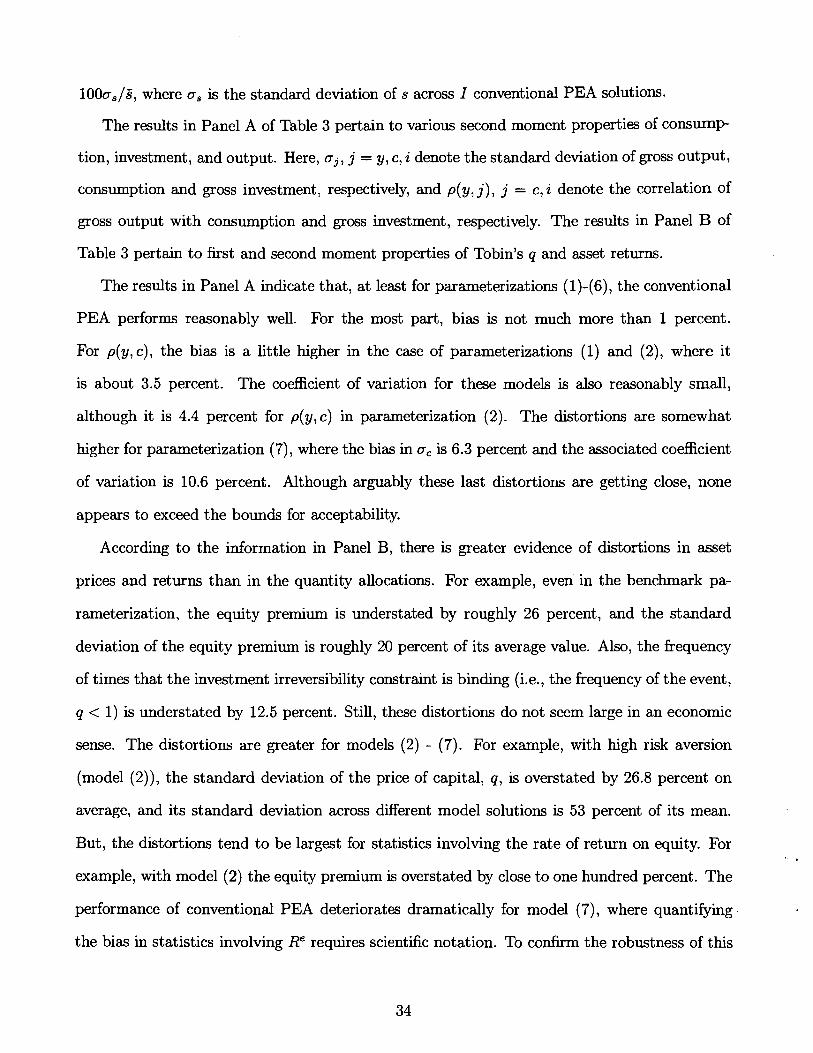
100a,/~, where a, is the standard deviation of s across I conventional PEA solutions.

The results in Panel A of Table 3 pertain to various second moment properties of consump

tion, investment, and output. Here, aj , j = y, c, i denote the standard deviation of gross output,

consumption and gross investment, respectively, and p(y, j), j = c, i denote the correlation of

gross output with consumption and gross investment, respectively. The results in Panel B of

Table 3 pertain to first and second moment properties of Tobin's q and asset returns.

The results in Panel A indicate that, at least for parameterizations (1)-(6), the conventional

PEA performs reasonably well. For the most part, bias is not much more than 1 percent.

For p(y, c), the bias is a little higher in the case of parameterizations (1) and (2), where it

is about 3.5 percent. The coefficient of variation for these models is also reasonably small,

although it is 4.4 percent for p(y, c) in parameterization (2). The distortions are somewhat

higher for parameterization (7), where the bias in a, is 6.3 percent and the associated coefficient

of variation is 10.6 percent. Although arguably these last distortions are getting close, none

appears to exceed the bounds for acceptability.

According to the information in Panel B, there is greater evidence of distortions in asset

prices and returns than in the quantity allocations. For example, even in the benchmark pa-

rameterization, the equity premium is understated by roughly 26 percent, and the standard

deviation of the equity premium is roughly 20 percent of its average value. Also, the frequency

of times that the investment irreversibility constraint is binding (i.e., the frequency of the event,

q < 1) is understated by 12.5 percent. Still, these distortions do not seem large in an economic

sense. The distortions are greater for models (2) - (7). For example, with high risk aversion

(model (2)), the standard deviation of the price of capital, q, is overstated by 26.8 percent on

average, and its standard deviation across different model solutions is 53 percent of its mean.

But, the distortions tend to be largest for statistics involving the rate of return on equity. For

example, with model (2) the equity premium is overstated by close to one hundred percent. The

performance of conventional PEA deteriorates dramatically for model (7), where quantifying

the bias in statistics involving Re requires scientific notation. To confirm the robustness of this

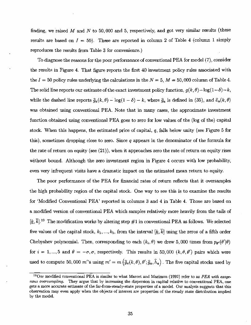
finding, we raised M and N to 50,000 and 5, respectively, and got very similar results ( thee

results are based on I = 50). These are reported in column 2 of Table 4 (column 1 simply

reproduces the results from Table 3 for convenience.)

TO diagnose the reasons for the poor performance of conventional PEA for model (7), consider

the results in Figure 4. That figure reports the f is t 40 investment policy rules associated with

the I = 50 policy rules underlying the calculations in the N = 5, M = 50,000 column of Table 4.

The solid line reports our estimate of the exact investment policy function, g (k, 8) - log(1- 6) - k,

while the dashed line reports ca(k, 8) - log(1 - 6) - k, where lja is defined in (35), and G(k, 8)

was obtained using conventional PEA. Note that in many cases, the approximate investment

function obtained using conventional PEA goes to zero for low values of the (log of the) capital

stock. When this happens, the estimated price of capital, q, falls below unity (see Figure 5 for

this), sometimes dropping close to zero. Since q appears in the denominator of the formula for

the rate of return on equity (see (21)), when it approaches zero the rate of return on equity rises

without bound. Although the zero investment region in Figure 4 occurs with low probability,

even very infrequent visits have a dramatic impact on the estimated mean return to equity.

The poor performance of the PEA for financial rates of return reflects that it oversamples

the high probability region of the capital stock. One way to see this is to examine the results

for 'Modified Conventional PEA' reported in columns 3 and 4 in Table 4. Those are based on

a modified version of conventional PEA which samples relatively more heavily from the tails of

[k, X].'"he modification works by altering step #1 in conventional PEA as follows. We selected

five values of the capital stock, kl, ..., kg, from the interval [k,x] using the zeros of a fifth order

Chebyshev polynomial. Then, corresponding to each (k,, 8) we drew 5,000 times from Pet (O'le)

for i = 1, ..., 5 and 8 = -17, o, respectively. This results in 50,000 (k, 8,8') pairs which were

used to compute 50,000 m"s using m' = m (ca (k, 8) ,8'; $, ^ha) . The five capital stocks used by

'"ur modified conventional PEA is similar to what Marcet and Marimon (1992) refer to as PEA with exoge- nous oversampling. They argue that by increasing the dispersion in capital relative to conventional PEA, one gets a more accurate estimate of the far-from-steady-state properties of a model. Our analysis suggests that this observation may even apply when the objects of interest are properties of the steady state distribution implied by the model.

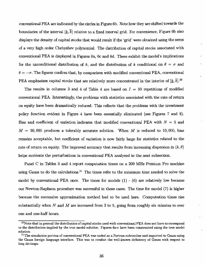
conventional PEA are indicated by the circles in Figure 6b. Note how they are shifted towards the

boundaries of the interval [b, x] relative to a fixed interval grid. For convenience, Figure 6b also

displays the density of capital stocks that would result if the 'grid' were obtained using the zeros

of a very high order Chebyshev polynomial. The distribution of capital stocks associated with

conventional PEA is displayed in Figures 6a,.6c and 6d. These exhibit the model's implications

for the unconditional distribution of k, and - the distribution of k conditional on 9 = a and

9 = -a. The figures confirm that, by comparison with modified conventional PEA, conventional

- 20 PEA emphasizes capital stocks that are relatively more concentrated in the interior of [b, k].

The results in columns 3 and 4 of Table 4 are based on I = 50 repetitions of modified

conventional PEA. Interestingly, the problems with st atistics associated with the rate of return

on equity have been dramatically reduced. This reflects that the problems with the investment

policy function evident in Figure 4 have been essentially eliminated (see Figures 7 and 8).

Bias and coefficient of variation indicates that modified conventional PEA with N = 5 and

M = 50,000 produces a tolerably accurate solution. When M is reduced to 10,000, bias

remains acceptable, but coefficient of variation is now fairly large for statistics related to the

rate of return on equity. The improved accuracy that results from increasing dispersion in (k, 9)

helps motivate the perturbations in conventional PEA analyzed in the next subsection.

Panel C in Tables 3 and 4 report computation times on a 200 MHz Pentium Pro machine

using Gauss to do the ~alculations.~' The times refer to the minimum time needed to solve the

model by conventional PEA once. The times for models (1) - (6) are relatively low because

our Newton-Raphson procedure was successful in these cases. The time for model (7) is higher

because the successive approximation method had to be used here. Computation times rise

substantially when N and M are increased from 3 to 5, going from roughly six minutes to over

one and one-half hours.

20Note that in general the distribution of capital stocks used with conventional PEA does not have to correspond to the distribution implied by the true model solution. Figures 6a-c have been constructed using the true model solution.

2 1 ~ h e simulation portion of conventional PEA was coded as a Fortran subroutine and imported to Gauss using the Gauss foreign language interface. This was to combat the well-known deficiency of Gauss with respect to long do-loops.

5.2.2. Chebyshev PEA

Approximating Marcet 's Conditional Expectat ion Function by PEA Collocation

We applied PEA collocation to approximate e in a l l seven models, and obtained acceptable

accuracy with N = M = 3 for models (1) to (6). By 'acceptable', we mean that all statistics

analyzed in Table 3 and 4 are within 10 percent of their exact values. We only study bias for this

method, since Monte Carlo uncertainty is not applicable. ~ l t h o u ~ h ' a c c u r a c ~ for models (1) to

(6) was comparable to that obtained by conventional PEA, computation times were drastically

lower, closer to one-half second instead of one-half minute or more. To save space, we do not

discuss these results and we instead focus on the analysis of model (7).

The last two columns of Table 4 report results using PEA collocation to approximate the

function, e, for model (7). In these columns, we set N, M to 3 and 5, respectively. Figure 9

exhibits the impact of increasing N and M on the Euler errors, RPea(k, 6; 6,) (see (13)). Since the

errors are difficult to interpret .directly, we convert them into the percent change in consumption

needed to make the Euler error zero, holding Tobin's q and the level of investment un~hanged.'~

A notable feature of Figure 9 is that the Euler errors are very small for N = M = 3. For

example, according to Figure 9, when 6 = -a the N = M = 3 rule fails the first order condition

by only one, one-hundredth of a percent of consumption. When 6 = a the rule fails by only

six, one-thousandths of a percent of current consumption. These are tiny numbers and yet the

N = M = 3 rule does not produce acceptable accuracy (see Table 4.) To get the desired degree

of accuracy, one has to go to N = M = 5. We conclude that a researcher interested in financial

statistics really must work to make the Euler errors extremely small.

Evidently, the performance of PEA collocation with M = 5, N = 5 is comparable or better

than that of conventional PEA with M = 50,000, N = 5, even though the former uses 10,000

times fewer observations than the latter. This difference is reflected in the amount of computer

2 2 ~ e t c denote the level of consumption in the approximate solution and let 2: denote the level of con- sumption needed to set the Euler error to zero without changing either the level of investment or To- bin's q. We have C-7 - ka(k, e) = qc-7 = Pexp (Ca(k, e ) ) , and 2: is defined by the relation, 2:-7q = P [exp (Ea(k, 8) - RPea(k, 8; C,))] . Dividing and rearranging, we get our consumption-based measure of the Euler error: 100 (Z/c - 1) = 100 [exp (RPea(k, 8; Ca)/-y) - I.] .

time required to solve the model. Whereas conventional PEA requires over one and one-half

hours to solve the model, PEA collocation requires a little over one-half of a second to get the

same degree of accuracy.

Two Further Experiments with Chebyshev PEA

Continuous Exogenous Shock

We considered two other sets of experiments with PEA collocation. In the first we consider

a version of Model (1) in which the technology shock has a continuous, normal distribution. We

did this out of a concern that the experiments in Tables 3 and 4 might be conferring too great

an advantage to PEA collocation, over conventional PEA. PEA collocation is in fact compatible

with evaluating integrals like those in (9), (14) and (16) by any method whatever, including

Monte Carlo methods. However, in most of the experiments with PEA collocation reported

in this paper, these integrals were evaluated exactly by fully exploiting the particular two-state

distribution assumed for the technology shock. Conventional PEA was not given this advantage.

The Monte Carlo method it applies to evaluate these integrals makes no use whatever of the

structure of the shock distribution. To verify that our results are not unduly influenced by

this asymmetry of treatment, we also did two experiments with versions of Model (1) in which

the technology shock has a continuous distribution. The results are reported in Table 5. The

column labelled 'benchmark' corresponds to the case in which the shock is iid over time, while

the other column corresponds to the case in which the shock has autocorrelation, p, equal to

0.95. The integral in (14) was evaluated using H -point Gauss-Hermite quadrature integration,

with H = 4 in each case. The table shows the values of N and M used for conventional PEA and

Chebyshev PEA needed to achieve acceptable accuracy, as well as the time needed to execute

the computations. The results are consistent with our previous findings. Namely, to get a

given degree of accuracy with Chebyshev PEA or PEA collocation requires at least an order of

magnitude less computation time than does conventional PEA.

Approximating the Wright- Williams Conditional Expectation

For our second set of experiments, we applied PEA collocation to approximating the condi-

tional expectation function, exp [v(kl, O ) ] , emphasized by Wright and Williams (1982a, 1982b,

1984). We address two issues raised in our discussion after (15)-(18): (i) we investigate whether

the various potential pathologies discussed there are likely to occur in practice, and (ii) we in-

vestigate the relative smoothness of the e and v functions. We work with the benchmark model,

Model (I) , and set N = M = 5. Since that model assumes an iid technology shock, 8 is not an

argument of v. Consequently, application of PEA collocation requires determining the values of

only 5 parameters and not the 10 needed to approximate e when N = 5.

Our results are displayed in Figure 10. To help assess the accuracy of the calculations,

Figure 10a displays the Euler errors, measured in the same units as the errors in Figure 6. The

continuous curve indicates the Euler errors over a very fine grid, and the stars indicate the

location of the five grid capital grid points used in the ~alculat ions.~~ The PEA collocation

method forces the Euler errors to be zero at these points. The largest error occurs for k slightly

above 4 and is nearly six one hundretbs of percent of consumption. The results in Figure 10b

allow us to consider issue (i). It displays the initial and final 6, functions in the sequence of

functions produced in the calculations. As in all other calculations in the paper, the initial

function is the one associated with a zero multiplier function and the log-linearized steady

state investment function, truncated so that gross investment is non-negative. The approximate

solution was found by initiating the calculations with 10 successive approximation steps, followed

by switching to a Newton-Raphson procedure. All functions in the sequence generated by this

approach are monotonically decreasing, and they rotate smoothly from the initial relatively

flat one to the steeper one where the calculations terminated. The fact that these functions

are monotonically decreasing is significant, since it establishes that we avoided the various

pathologies discussed after (15)- (1 8).

Figures 10c - 10f allow us to address issue (ii), concerning the relative smoothness of

v(kl, 8) versus that of e(k, 8) = v (g(k, 8), 8) . To assess the relative smoothness of these two

'"he interval width for the fine grid used in Figure 10 is 0.005.

functions, we cornpare E(k, 6; a) = log [J m (ij,(k, 6) ,6'; &, ha) (6' I 6)d6'] and V(kl; a)

log [J m (kt, 8'; ija, ha) pol (6 I 8)d8'] , where $ and b are derived from our approximate solution,

6,. Two sets of observations are relevant in assessing the relative smoothness of E and V. The

first can be seen in Figures 10c and 10d, which display gross investment, ij,(k, 8) - log(1- 6) - k,

for the two lowest values of 8 used in the Gauss-Hermite quadrature calculations. Evidently,

the slope of lja(k, 8) undergoes an abrupt jump at the value of the capital stock where the irre-

versibility constraint becomes binding, a value that is increasing with 8. The second observation

is that the function V appears to be quite smooth. This can be seen in Figures 10e and 10f,

which plot dV(kl; a)/dkl against 'These properties of V and ij, suggest that V is smoother

than E . In particular, they indicate that E must have a kink at the point were the irreversibility

constraint becomes binding, since E (k, 6; a) = V(ij,(k, 8); a).

The presumed lack of smoothness in E(k, 6; a) is too slight to be visible in a graph of E

against k. However, it is evident in the graph of the slope of E . This can be seen in Figures

10e and 10f, which graph dE(k, 6; a)/dk against k for the same two values of 6 used in Figures

lob and 10c. It is not surprising that the slopes of E and V coincide in the region where the

irreversibility constraint is binding, since the derivative of g,(k, 8) with respect to k is unity

there. Moreover, in light of the negative sign in the slope of V and the fact that the slope of ij,

jumps when the irreversibility constraint begins to bind, it is also not surprising that the slope

of E(k, 6; a) falls abruptly at this value of k. These observations are consistent with the remarks

after equation (20), suggesting that v is a smoother function than e, and therefore easier to

approximate numerically.

5.3. Comparing the Algorithms

In this section we compare five algorithms in terms of their ability to acheve a given degree of

accuracy and the minimum computer time they need to accomplish this. The target degree of

accuracy that we consider is that a solution imply a set of values for the 11 statistics studied

24~n this and the next paragraph, df (x ) /dx means [f ( x ) - f ( x - E ) ] / E for E = 0.005.

in Tables 3 and 4 that come within at least 10% of the corresponding exact values obtained by

dynamic programming. Our findings are based principally on the results reported in Table 6.

Apart from the results corresponding to conventional PEA, results not in parentheses in that

table are the minimal computer time achevable by some choice of algorithm parameters for

the solution to achieve the accuracy criterion. Results for conventional PEA simply report the

time needed to compute the solution with .N = 3 and M = 10,000, without regard to accuracy.

Computing minimal times for conventional PEA was impractical. The Monte Carlo aspect of

the method implies that analyzing it requires computing a large set of solutions for each N and

M. Other details about the computations are reported in the notes to' the table.

Three things are worth noting about the results. First, PEA collocation is able to achieve

the target degree of accuracy at least ten times faster than any other algorithm. Second,

one of the algorithms, spectral Galerkin, actually failed to achieve a solution for two of the

parameterizations. Third, though it is not evident from Table 6, conventional PEA also fails to

meet the accuracy test at least for model (7). Table 4 shows that conventional PEA with N = 3,

M = 10,000 and N = 5, M = 50,000 violates our accuracy criterion. In addition, in results

not shown, we get a little closer to the accuracy target with N = 3, M = 50,000, but bias in

the return on equity is still over 40 percent and the associated coefficient of variation is over 70

percent in this case.25 Although Table 4 shows that modified conventional PEA improves on

the accuracy of conventional PEA, when N = 5, M = 50,000 and N = 5, M = 10,000, it too

fails to meet our accuracy criterion.

6. Concluding Remarks

Our purpose in this paper is to provide information useful to researchers for selecting one of

the many available solution algorithms for solving dynamic models with occasionally binding

constraints. In our analysis of algorithms, the criteria we consider include computational speed,

25These results are consistent with den Haan (1995)'s finding that he needed very high values of M to get accurate solutions for rates of return with conventional PEA.

programming convenience and numerical accuracy.

The different algorithms studied exploit the various ways that exist for characterizing a

model solution. In all cases, the characterization takes the form of the requirement that a

particular functional equation be zero over the domain of the capital stock and the support of

the exogenous disturbance. We consider algorithms that exploit characterizations based on the

Lagrange multiplier and penalty function representations of the solution, and also algorithms .

that characterize the solution in terms of a conditional expectation function. The algorithms

differ greatly in terms of the criteria considered. The ones that work best in our application -

solving the stochastic growth model with irreversible investment - are a subset of the ones based

on characterizing the solution in terms of a conditional expectation. We assessed the accuracy

of the algorithms based on their implications for first and second moment properties of real

quantities and financial statistics, including the rate of return on equity. The properties of the

latter turned out to be the hardest to approximate well, and it is with this variable that the

accuracy advantages of a subset of the PEAS manifested itself most clearly.

The best known PEA in applied macroeconomics is the one due to Marcet (1988), which

we call conventional PEA. We describe an alternative algorithm, called Chebyshev PEA, which

improves upon some deficiencies of Marcet's PEA. In addition, we study a PEA proposed in

earlier work by Wright and Williams (1982a71982b71984). The conditional expectation approx-

imated by Wright and Williams' PEA is attractive from a computational point of view because

it is smooth compared to the function approximated in conventional PEA. At the same time,

we show that Wright and Williams' PEA can in principle have other problems. We show that

those problems do not actually arise in the analysis of the one sector growth model. Still, they

may be of concern in other applications.

In our analysis we were able to evaluate the accuracy of alternative algorithms because of the

simplicity of the model economy studied. This allowed us to develop, for comparison purposes,

a very accurate approximation to the model solution using dynamic programming methods. Of

course, in practice this way of assessing accuracy is not available. In a typical application, the

best one can do is to attempt to study how successful an algorithm is in driving the relevant

functional equation close to zero. We tried to shed light on how close to zero one needs to be

to get acceptable accuracy. In our applications, the relevant functional equation corresponds to

the Euler error of a planner's first order condition, expressed as a function of the state.26 We

found.that to get acceptable accuracy for financial rates of return, especially the rate of return

on equity, requires extraordinarily small Euler errors. We measured the error for a particular .

value of the capital stock and exogenous shock by the percent change in consumption needed

to drive that error to zero. We studied one approximate solution in which the maximum Euler

error was only 0.012 percent of consumption, and yet there was still an unacceptable 30 percent

bias in the mean return on equity.

Although we considered a wide range of parameter values for our model, it bears emphasiz-

ing that we have not established that our findings regarding the advantages of various PEAS

apply generally.27 Confidence that results like these hold more generally requires building up

experience over time with a variety of applications. We think that further research along these

lines would be useful.

2GSantos (1997a) takes some steps in the direction of developing formal methods for using Euler equation errors to assess the accuracy of an approximation. He does not consider the case of occasionally binding constraints studied here. In addition, in assessing accuracy we focus on implications for second moment properties, while Santos focuses on implications for policy rules.

27An exception, noted in the introduction, is that we do show that the linearity and orthogonality properties of Chebyshev PEA apply in arbitrary dimensions.

References

[:I.] Aiyagari, S. Rao. 1993. Frictions in Asset Pricing and Macroeconomics. European Economic Review, 38, pp. 932-39.

[2] Aiyagari, S. Rm, Zvi Eckstein, and Martin Eichenbaurn. 1980. Rational Expectations, Inventories and Price Fluctuations. Yale University, Economic Growth Center Discussion Paper 363, October.

[3] Aiyagari, S. Rao and Mark Gertler. 1991. Asset Returns With Transactions Costs and Uninsured Individual Risk. Journal of Monetary Economics, 27: 311-331.

[4] Atkeson, Andy and Patrick Kehoe. 1993. Industry Evolution and Transition: The Role of Information Capital. Manuscript.

[5] Bizer, David S., and Kenneth L. Judd. 1989. Uncertainty and Taxation. American Economic Review, Papers and Proceedings, May.

[6] Boldrin, Michele, Lawrence J. Christiano, and Jonas D.M. Fisher. 1994. Habit Persistence and the Equity Premium in the Neoclassical Growth Model. Manuscript.

[7] Chari, V.V., Lawrence J. Christiano, and Patrick Kehoe. Forthcoming. "Policy Analysis in Business Cycle Models", in Cooley, editor, Frontiers of Business Cycle Research, Princeton University Press, Princeton, NJ.

[8] Christiano, Lawrence J. 1991. Modeling the Liquidity Effect of a Monetary Shock. Federal Reserve Bank of Minneapolis Quarterly Review 15 (Winter): 3-34.

[9] Christiano, Lawrence J. and Terry Fitzgerald. 1991. The Magnitude of the Speculative Mo- tive for Holding Inventories in a Business Cycle Model. Federal Reserve Bank of Minneapolis Working Paper 415.

[lo] Coleman, Wilbur John. 1988. Money, Interest and Capital in a Cash-in-Advance Economy. International Finance Discussion Paper No. 323. Washington: Board of Governors, Federal Reserve System.

[ll.] Coleman, Wilbur John. 1996. The Behavior of Interest Rates In a General EQuilibrium, Multisector Model with Irreversible Investment. Manuscript, Fuqua School of Business, Duke University.

[12] Coleman, Wilbur John, and Ming Liu. 1997. Incomplete Markets and Inequality Con- straints: Some Theoretical, Computational, and Empirical Issues. Manuscript, Fuqua School of Business, Duke University.

[13] Coleman, Wilbur John, Christian Gilles, and Pamela Labadie. 1992. The Liquidity Premium in Average Interest Rates. Journal of Monetary Economics, 30: 449-465.

[14] Danthine, Jean-Pierre and John B. Donaldson. 1981. Stochastic Properties of Fast vs. Slow Growing Economies. Econornetrica 49: 1007-1033.

[15] den Haan, Wouter. 1993. Heterogeneity, Aggregate Uncertainty and'the Short Term Interest Rate: A Case Study of Two Solution Techniques. University of California at San Diego Manuscript.

[16] den Haan, Wouter. 1995. The Term Structure of Interest Rates in Real and Monetary 4

Economies. Journal of Economic Dynamics and Control, vol. 19, no. 5-7, July-September.

[17] den Haan, Wouter and Albert Marcet. 1990. Solving the Stochastic Growth Model by Parameterizing Expectations. Journal of Business and Economic Statistics 8: 31-34.

[18] den Haan, Wouter, Gary Rarney, and Joel Watson. 1997. Job Destruction and Propagation of Shocks. manuscript, UCSD.

[19] den Haan, Wouter and Albert Marcet. 1994. Accuracy in Simulation. Review of Economic Studies, vol. 61 (I) , no. 206, pp. 3-18, January.

[2C)] den Haan, Wouter. 1996. Understanding Equilibrium Models with a Small and a Large Number of Agents. NBER working paper #5792.

[21] den Haan, Wouter. 1997, Solving Dynamic Models with Aggregate Shocks and Heteroge- neous Agents. Macroeconomic Dynamics, forthcoming.

[22] Gomme, Paul. 1997. Evolutionary Programming as a Solution Technique for the Bellman Equation. Unpublished manuscript Federal Reserve Bank of Cleveland.

[23] Greenwood, J., G.M., MacDonald, G-J Zhang. 1996. The Cyclical Behavior of Job Creation and Job Destruction: A Sectoral Model. Economic Theory, 7, pp. 95-112.

[24] Gustafson, Robert L. 1958. Carryover Levels for Grains: A Method for Determining Amounts that are Optimal Under Specified Conditions. Technical Bulletin No. 1178, US Department of Agriculture, Washington, D. C.

[25] Heaton, John and Deborah Lucas. 1992. The Effects of Incomplete Insurance Markets and Trading Costs in a Consumption-Based Asset Pricing Model. Journal of Economic Dynamics and Control, 16: 601-620.

[26] Heaton, John and Deborah Lucas. 1996. Evaluating the Effects of Incomplete Markets on Risk Sharing and Asset Pricing. Journal of Political Economy, 104, pp. 443-87.

[27] Huggett , Mark. 1993. The Risk-Ree Rate in Heterogeneous- Agent Incomplete-Insurance Economies. Journal of Economic Dynamics and Control, 17: 953-969.

[28] Judd, Ken. 1991. Minimum Weighted Residuals Methods for Solving Aggregate Growth Models. Institute for Empirical Macroeconomics Discussion Paper No. 49.

[29] Judd, Ken. 1992a. Projection Met hods for Solving Aggregate Growth Models. Journal of Economic Theory, 58: 410-452.

[30] Judd, Ken. 1992b. Numerical Methods in Economics. Manuscript.

[31] Judd, Ken. 1993. Comments on ~ a r c e t , Rust and Pakes. Forthcoming comments made at the World Congress of the Econometric Society, Barcelona.

[32] Judd, Ken and Antonio Bernardo. 1994. Projection Methods for Computing Conditional Expectations. Stanford University Working Paper.

[33] Kahn, James. 1992. Why is Production More Volatile than Sales? Theory and Evidence on the Stock-out Avoidance Motive for Inventory Holding. Quarterly Journal of Economics, 107: 481-510.

[34] Kiyotaki, Nobuhiro and John Moore. 1993. Credit Cycles. Manuscript.

[35] Lucas, Deborah. 1994. Asset Pricing with Undiversifiable Income Risk and Short Sales Constraints: Deepening the Equity Premium Puzzle. Journal of Monetary Economics, 34, pp. 325-41

[36] Luenberger, David. 1969. Optimization by Vector Space Methods. New York: John Wiley & Sons.

[37] Marcet, Albert. 1988. Solving Nonlinear Stochastic Growth Models by Parametrizing Ex- pectations. Carnegie-Mellon University, mimeo.

[38] Marcet , Albert and Juan Ketterer. 1989. Introducing Derivative Securities: A General Equilibrium Approach. Carnegie-Mellon University Working Paper.

[39] Marcet, Albert and Ramone Marimon. 1992. Communication, Committment and Growth. Journal of Economic Theory, 58: 219-249.

[40] Marcet, Albert and David Marshall. 1994. Solving Non-linear Rational Expectations Models by Parameterized Expectations; Convergence to Stationary Solutions. Universitat Pompeu Fabra Working paper number 76, Barcelona.

[41] Marcet, Albert and Ken Singleton. 1990. Equilibrium Asset Prices and Savings of Hetero- geneous Agents In the Presence of Portfolio Constraints. Unpublished manuscript.

[42] Marshall, David. 1992. Inflation and Asset Returns in a Monetary Economy. Journal of Finance, 47: 1315-42.

[43] McCurdy, Tom and Nicholas Ricketts. 1995. An international economy with country-specific money and productivity growth processes. Canadian Journal of Economics, 28, pp. 141-62.

[44] McGrattan, Ellen. 1993. Solving the Stochastic Growth Model with a Finite Element Method. Federal Reserve Bank of Minneapolis mimeograph.

[45] Miranda, Mario J. 1985. Analysis of Rational Expectations Models for Storable Com- modities Under Government Regulation. Unpublished doctoral dissertation, University of Wisconsin-Madison.

[46] Miranda, Mario J., and Peter G. Helmberger. 1988. The Effects of Commodity Price Sta- bilization Programs. American Economic Review, vol. 78, no. 1, pp. 46-58.

[47] Press, William H., Saul Teukolsky, William Vetterling, and Brian Flannery. 1992. Numerical Recipes in Fortran. New York: University of Cambridge Press.

[48] Reddy, J.N. 1993. An Introduction to the Finite Element Method. New York: McGraw-Hill.

[49] Rust, John. 1996. Numerical Dynamic Programming in Economics, in H. Amman, D. Kendrick and J. Rust, editors, Handbook of Computational Economics, Elsevier, North Holland, forthcoming.

<

[50] Santos, Manuel, 1997a, 'An Accuracy Test Using the Euler Equation Residuals,' manu- script, University of Minnesota.

[5:1.] Santos, Manuel, 1997b, 'Numerical Solution of Stochastic Growth Models,' manuscript, University of Minnesota.

1521 Sargent, Thomas. 1980. Tobin's q and the Rate of Investment in General Equilibrium. Carnegie-Rochester Conference Series on Public Policy 12.

[53] Stockman, David R. 1997. Balanced-Budget Rules: Welfare Consequences, Optimal Poli- cies, and Theoretical Implications. Unpublished University of Chicago doctoral dissertation.

[54] Stokey, Nancy and Robert E. Lucas, Jr., with Edward Prescott. 1989. Recursive Methods in Economic Dynamics. Cambridge, MA: Harvard University Press.

[55] Stroud, A.H. 1971. Approximate Calculation of Multiple Integrals. Englewood Cliffs, NJ: Prentice-Hall.

[56] Taylor, John, and Harald Uhlig. 1990. Solving Nonlinear Stochastic Growth Models: A Comparision of Alternative Solution Methods. Journal of Economics and Business, 8, pp. 1-17.

[57] Telmer, Chris. 1993. Asset Pricing Puzzles and Incomplete Markets. Journal of Finance, 48, 1803-32.

[58] Wright, Brian D., and Jeffrey C. Williams. 1982a. The Economic Role of Commodity Stor- age. Economic Journal, 92 pp. 596-614.

[59] Wright, Brian D., and Jeffrey C. Williams. 1982b. The Roles of Public and Private Storage in Managing Oil Import Disruptions. Bell Journal of Economics 13, pp. 341-353.

[60] Wright, Brian D., and Jeffrey C. Williams. 1984. The Welfare Effects of the Introduction of Storage. Quarterly Journal of Economics, 99, pp. 169-182.

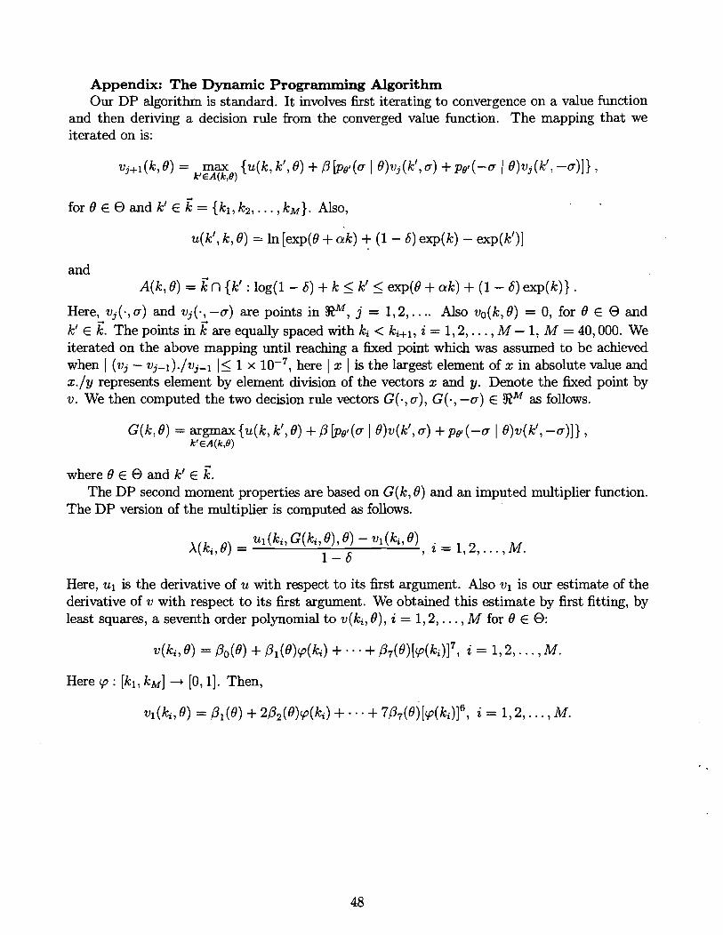
Appendix: The Dynamic Programming Algorithm Our DP algorithm is standard. It involves first iterating to convergence on a value function

and then deriving a decision rule from the converged value function. The mapping that we iterated on is:

for8 E 8 and k t € E = {kl,k2 ,..., kM) Also,

and A(k, 8) = I n {kt : log(1- 6) + k < k' < exp(8 + ale) + ( I - 6) exp(k))

Here, vj(-, a) and v.(. -a) are points in RM, j = 1,2,. . .. Also vo(k, 8) = 0, for 8 E 8 and 1. kt E L The points in k are equally spaced with k; < ki+l, i = 1,2,. . . , M - 1, M = 40,000. We iterated on the above mapping until reaching a fixed point which was assumed to be achieved when ( (vj - ~ j - ~ ) . / ~ j - ~ I < 1 x here I x 1 is the largest element of x in absolute value and x./y represents element by element division of the vectors x and y. Denote the fixed point by v. We then computed the two decision rule vectors G(- , a), G(. , -a) E RM as follows.

where 8 E C3 and kt E z. The DP second moment properties are based on G(k, 8) and an imputed multiplier function.

The DP version of the multiplier is computed as follows.

Here, u1 is the derivative of u with respect to its first argument. Also vl is our estimate of the derivative of v with respect to its first argument. We obtained this estimate by first fitting, by least squares, a seventh order polynomial to v(k,, 8)) i = 1,2,. . . , M for 8 E 8 :

Here cp : [kl, kM] --+ [O, 11. Then,

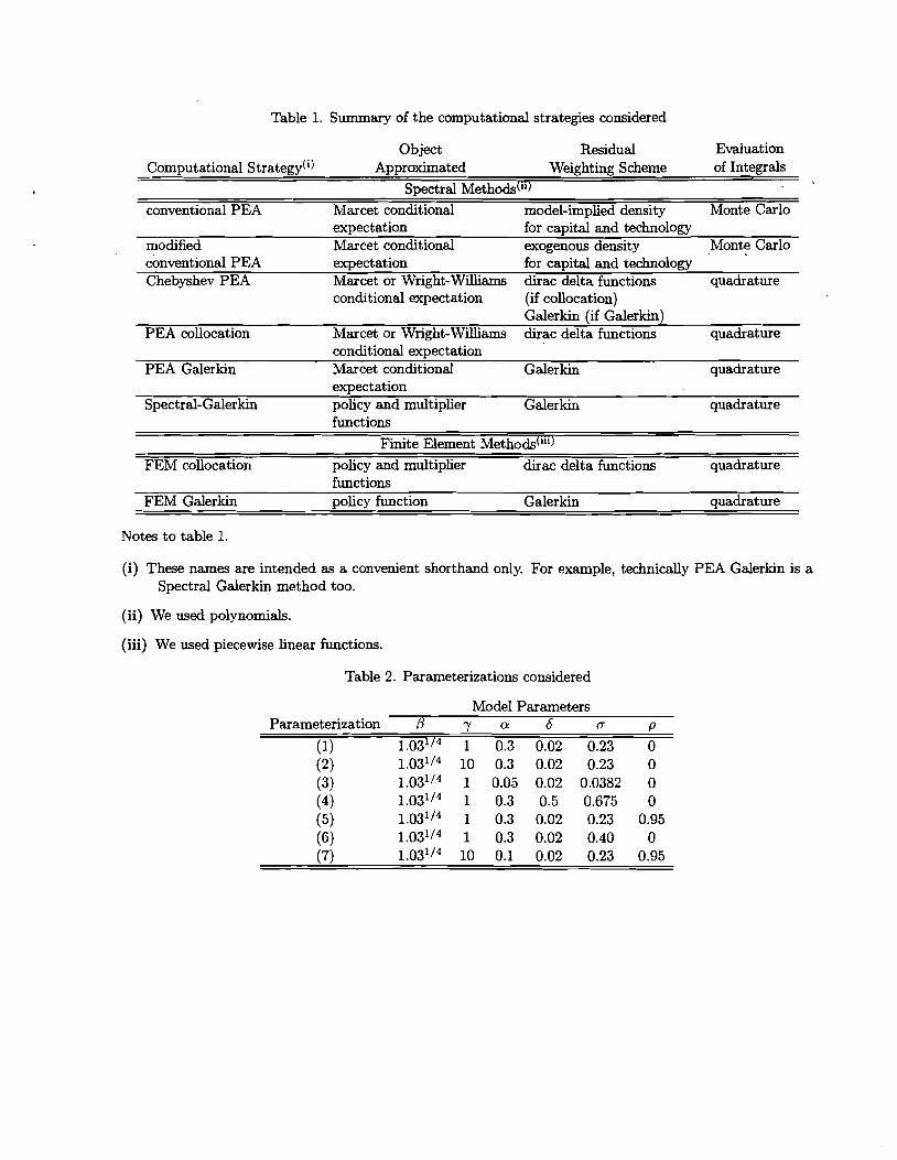
Table 1. Summary of the computational strategies considered

Object Residual Evaluation Computational Strategy(') Approximated Weighting Scheme of Integrals

conventional PEA Marcet conditional model-implied density Monte Carlo expectation for capital and technblogy

modified Marcet conditional exogenous density Monte Carlo conventional PEA expectation for capital and technology Chebyshev PEA Marcet or Wright-Williams dirac delta functions quadrature

conditional expectation (if collocation) ~a le rk in (if k e r k i n )

PEA collocation Marcet or Wright-Williams dirac delta functions quadrature conditional expectation

PEA Galerkin Marcet conditional Galerkin quadrature expectation

Spectral-Galerkin policy and multiplier Galerkin quadrature functions

Finite Element Methods("')

FEM collocation policy and multiplier dirac delta functions quadrature functions

FEM Galerkin policy function Galerkin quadrature

Notes to table 1.

(i) These names are intended as a convenient shorthand only. For example, technically PEA Galerkin is a Spectral Galerkin method too.

(ii) We used polynomials.

(iii) We used piecewise linear functions.

Table 2. Parameterizations considered

Model Parameters Parameterization 4 y cr b (7 P

(1) 1 . 0 3 ~ 1 ~ 1 0.3 0.02 0.23 0 (2) 1 . 0 3 ~ 1 ~ 10 0.3 0.02 0.23 0 (3) 1.03'1~ 1 0.05 0.02 0.0382 0 (4) 1 . 0 3 ~ 1 ~ 1 0.3 0.5 0.675 0 (5) 1 . 0 3 ~ 1 ~ 1 0.3 0.02 0.23 0.95 (6) 1.03l/~ 1 0.3 0.02 0.40 0 (7) 1.03'/~ 10 0.1 0.02 0.23 0.95

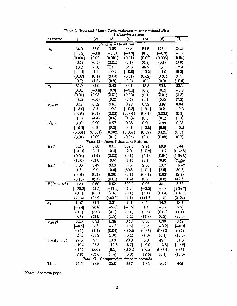
Table 3. Bias and Monte Carlo variation in conventional PEA Parameterizations

Statistic (1) (2) (3) (4) (5) (6) (7) Panel A - Quantities

'= Y 66.0 67.9 3.95 68.8 84.8 125.0 34.2 [-0.21 [-0.61 [-0.041 [-0.31 [O. l ] [-0.31 [-0.21 (0.004) (0.02) (0.001) (0.01) (0.02) (0.003) (0.04)

(0.1) (0.5) (0.01) (0.1) (0.5) (0.1) (0.9) 6, 10.2 7.50 1.01 34.3 49.7 45.4 12.4

[ O M ] [-0.81 [0.3] [-0.11 [0.3] [0.2] [-3.81 (0.01) (0.03) (0.01) (0.02) (0.1) (0.01) (0.3) (0.2) (0.6) (0.2) (0.4) (1.4) (0.3) (7.3)

P(Y 9 c ) 0.47 0.32 0.61 0.98 0.92 0.98 0.94 [-3.01 [3.5] [-0.31 [-0.31 [-0.11 [0.2] [-0.21 (0.05) (0.2) (0.02) (0.001) (0.01) (0.002) (0.1) (1.1) (4.4) (0.5) (0.03) (0.3) (0.1) (1.1)

P(Y 3 2 ) 0.99 0.99 0.97 0.98 0.90 0.99 0.98 [-0.11 [0.40] [0.3] [O.Ol] [-0.51 [0.5] [-0.21 (0.001) (0.001) (0.002) (0.002) (0.02) (0.001) (0.03) (0.01) (0.02) (0.1) (0.04) (0.4) (0.02) (0.7)

Panel B - Asset Prices and Returns E Re 3.20 3.08 3.01 309.5 2.94 59.8 1.44

[-0.11 [25.1] [0.4] [2.0] [-0.21 [-1.71 [1.6e8] (0.05) (1.9) (0.02) (0.1) (0.1) (0.04) (1.6e8) (1.04) (33.6) (0.5) (1.1) (2.7) (0.9) (2124)

ERf 3.00 2.47 3.00 8.6 2.88 19.7 -5.42 [1.8] [9.0] [0.6] [30.3] [-0.11 [2.6] [36.8]

(0.01) (0.3) (0.001) (0.1) (0.01) (0.03) (2.7)

(2.4) (31.2) (1.0) (0.4) (7.6) (0.1) (14.5) l?req(q < 1) 24.6 9.2 19.9 20.3 3.8 49.7 31.0

[-12.51 [25.5] [-12.61 [6.7] [-2.01 [-3.81 [-7.21 (0.1) (3.0) (0.1) (0.04) (0.4) (0.004) (0.6) (2.9) (52.6) (1.5) (0.8) (12.6) (0.1) (13.3)

Panel C - Computation times in seconds Time 26.5 28.8 25.6 38.7 19.3 26.5 406

Notes: See next page.

Notes to table 3.

i. Unbracketed numbers: statistic, sdp, based on a single simulation of length 100,000 generated using dynamic programming solution.

ii. Square bracketed numbers: 100 . (3 - sdp)/sdp, where 3 is the mean of the statistic across I = 500 simulated data sets of length 100,000 observations each. Each of the I datasets was generated by a different conventional PEA solution. For model (7), 48 of the artificial datasets had to be discarded because the capital stock converged to zero.

iii. Round bracketed numbers: Monte Carlo standard error, 100 . u,/(I . sdp), for the object in square brackets. Here a, is the standard deviation of the statistic across I conventional PEA-generated datasets.

iv. Angular bracketed numbers: coefficient of variation, 100. a,/Z.

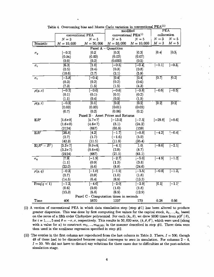
Table 4. Overcoming bias and Monte Carlo variation in conventional PEA(")

Statistic IM=lO,000 M = 5 0 , 0 0 0 M = 5 0 , 0 0 0 M = 1 0 , 0 0 0 1 M = 3 M = 5 1 Panel A - Quantities

modified conventional PEA

N = 3 N = 5

OY [-0.21 [0.2I 10.31 (0.31 [0.4] [0.3] (0.04) (0.03) (0.02) (0.07) (0.9) (0.2) (0.003) (0.5)

ac 16.31 [l-OI [-0.51 [-0.41 [-I .I.] [-0.31 (0.5) (0.4) (0.3) (0.8) (10.6) (2.7) (2.1) (5.9)

aa [-3.81 [-0.41 [0.41 [0.7] [0.2] (0.3) (0.2) (0.2) (0.6) (7.3) (1.5) (1.5) (4.3)

P(Y 7 c ) [-0.21 [-0.61 [-0.61 [-0.81 [-0.61 (-0.51 (0.1) (0.1) (0.1) (0.2) (1.1) (0.4) (0.5) (1.5)

P ( Y ~ i ) [-0.21 [O. I ] [0.21 IO.21 [0.2] [0.2] (0.03) (0.03) (0.01) (0.03) (0.7) (0.2) (0.06) (0.2)

Panel B - Asset Prices and Returns ERe [ I .6 e 81 [4.7e 71 [-13.01 [-7.51 [-29.81 [-8.61

(1.6e8) (4.6e 7 ) (8.1) (24.2)

PEA

(1.1) (0.9) (1-2) (3.3) (22.0) (6.6) (8-8) (24.6)

P(Y 7 9) [-0.31 [- 1 .O] [-1.91 [-3.51 [-0.81 [-1.21 (0.7) (0.9) (1.0) (1.8) (14.5) (6.4) (6.9) (13.3)

Fred9 < 1) [-7.21 [-4.61 [-2.01 [-3.91 [0.1] [-1.11 (0.6) (0.9) (1.0) (1.8) (13.3) (6.8) (6.9) (12.9)

Panel C - Computation times in seconds Time 406 5870 1237 170 0.28 0.66

conventional PEA(') N = 5 N = 5

(i) A version of conventional PEA in which data simulation step (step #1) has been altered to produce greater dispersion. This was done by first computing five values for the capital stock, k l , ..., k5, based on the zeros of a fifth order Chebyshev polynomial. For each (k i , e ) , we drew 5000 times from p(e' I e ) , for i = 1, ..., 5 and 8 = -a, a , respectively. This results in 50,000 sets, (k, 8, 8'), which were used (along with a value for a ) to construct mz, ..., mso,ool in the manner described in step #l. These data were then used in the nonlinear regression specified in step #2.

collocation N = 3 N = 5

(ii) The entries in the first column are reproduced from the last column in Table 3. There, I = 500, though 48 of these had to be discarded because capital converges to zero in simulation. For columns 2 - 4, I = 50. We did not have to discard any solutions for these cases due to difficulties at the post-solution simulation stage.

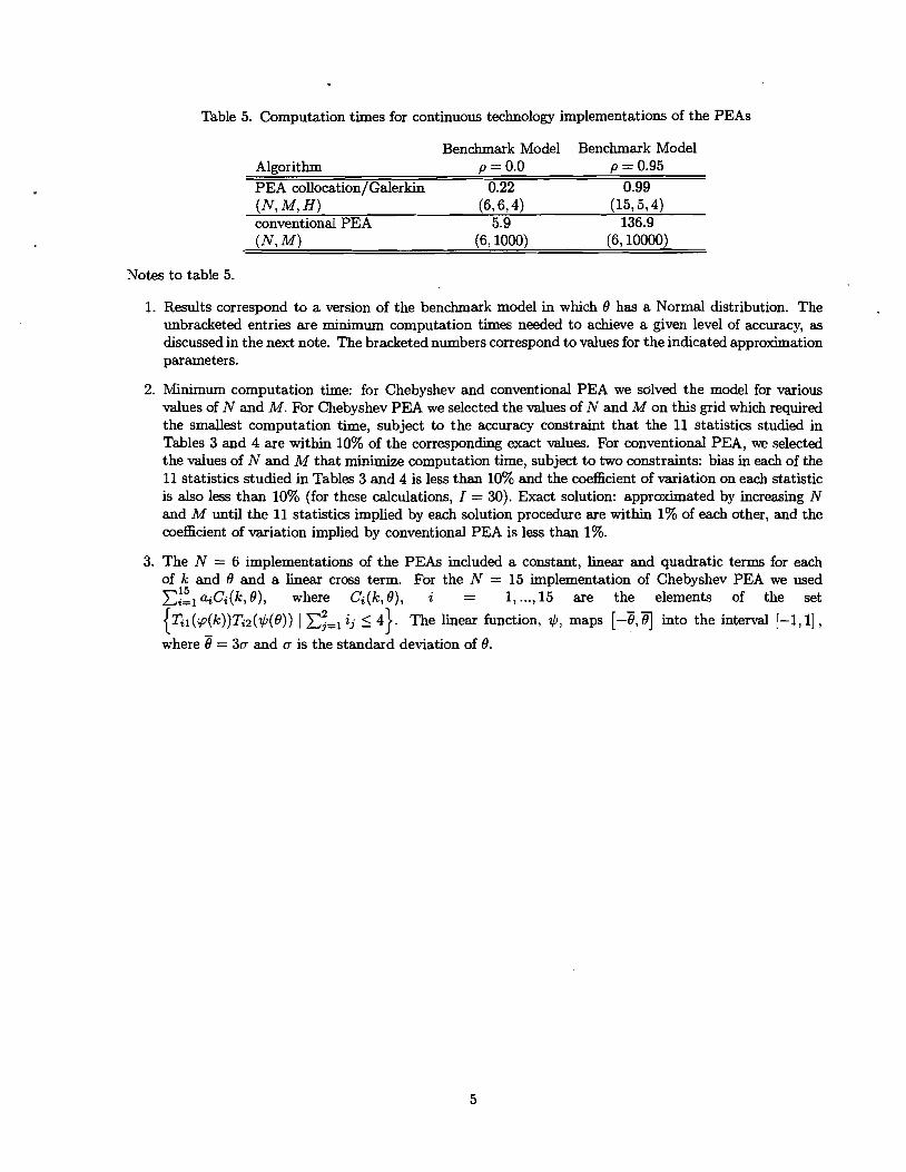
Table 5. Computation times for continuous technology implementations of the PEAS

Benchmark Model Benchmark Model Algorithm p = 0.0 p = 0.95 PEA collocation/Galerkin 0.22 0.99 (N, M, H) (6,674) (15,5,4) conventional PEA 5.9 136.9

. (N7M) (6,1000) (6,10000)

Notes to table 5.

1. Results correspond to a version of the benchmark model in which O has a Normal distribution. The unbracketed entries are minimum computation times needed to achieve a given level of accuracy, as discussed in the next note. The bracketed numbers correspond to values for the indicated approximation parameters.

Minimum computation time: for Chebyshev and conventional PEA we solved the model for various values of N and M. For Chebyshev PEA we selected the values of N and M on this grid which required the smallest computation time, subject to the accuracy constraint that the 11 statistics studied in Tables 3 and 4 are within 10% of the corresponding exact values. For conventional PEA, we selected the values of N and M that minimize computation time, subject to two constraints: bias in each of the 11 statistics studied in Tables 3 and 4 is less than 10% and the coefficient of variation on each statistic is also less than 10% (for these calculations, I = 30). Exact solution: approximated by increasing N and M until the 11 statistics implied by each solution procedure are within 1% of each other, and the coefficient of variation implied by conventional PEA is less than 1%.

3. The N = 6 implementations of the PEAS included a constant, linear and quadratic terms for each of k and O and a linear cross term. For the N = 15 implementation of Chebyshev PEA we used x:zl aiCi(k, O), where Ci(k, O), i = 1, ..., 15 are the elements of the set

{%I ( y ~ ( k ) ) ~ i ~ ( @ ( B ) ) I x:=l ij 5 4). The linear function, @, maps [-8,8] into the interval [-1,1] , where 8 = 3cr and a is the standard deviation of 0.

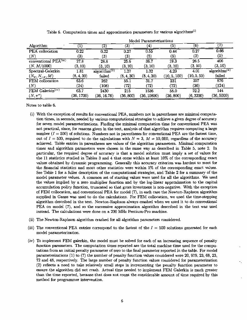
Table 6. Computation times and approximation parameters for various algorithmdi)

Model Pararneterizations

(N) (3) (3) (3) (5) (5) (3) (5) conventional PEA("') 27.8 28.8 25.6 38.7 19.3 26.5 406 - - -

(N, M/1000) (3,101 (3,101 (3,lO) (3,lO) (3,101 (3,lO) (3,lO) Spectral-Galerkin 1.81 algorithm(") 1.27 1.32 4.23 4.01 algorithm(") - (Nu, N-'7, M)

-

(8,4,30) failed . (8,4,30) (8,4,30) (10,5,100) (10,5,50) failed FEM collocation 63.6 262 55.1 31.7 23 1 207 876 (N) (24) (108) (72) (72) (72) (36) (124) FEM ~alerkid") 63.7 2430 215 1536 58.0 22.2 144

Notes to table 6.

(i) With the exception of results for conventional PEA, numbers not in parentheses are minimal computa- tion times, in seconds, needed by various computational strategies to achieve a given degree of accuracy for seven model parameterizations. Finding the minimal computation time for conventional PEA was not practical, since, for reasons given in the text, analysis of that algorithm requires computing a large number (I = 500) of solutions. Numbers not in parentheses for conventional PEA are the fastest time, out of I = 500, required to do the calculations with N = 3, M = 10,000, regardless of the accuracy achieved. Table entries in parentheses are values of the algorithm parameters. Minimal computation times and algorithm parameters were chosen in the same way as described in Table 5, note 2. In particular, the required degree of accuracy is that a model solution must imply a set of values for the 11 statistics studied in Tables 3 and 4 that come within at least 10% of the corresponding exact values obtained by dynamic programming. Generally this accuracy criterion was hardest to meet for the financial statistics and most other statistics were within 1% of the corresponding exact values. See Table 1 for a fuller description of the computational strategies, and Table 2 for a summary of the model parameter values. A common set of starting values were used for all the algorithms. We used the values implied by a zero multiplier function and by the log-linear approximation to the capital accumulation policy function, truncated so that gross investment is non-negative. With the exception of FEM collocation, and conventional PEA for model (7), in each case the Newton-Raphson algorithm supplied in Gauss was used to do the calculations. For FEM collocation, we used the time-stepping algorithm described in the text. Newton-Raphson always crashed when we used it to do conventional PEA on model (7), and so the successive approximation algorithm described in the text was used instead. The calculations were done on a 200 MHz Pentium-Pro machine.

(ii) The Newton-Raphson algorithm crashed for all algorithm parameters considered.

(iii) The conventional PEA entries correspond to the fastest of the I = 500 solutions generated for each model parameterization.

(iv) To implement FEM galerkin, the model must be solved for each of an increasing sequence of penalty function parameters. The computation times reported are the total machine time used for the compu- tations from an initial penalty parameter of zero to the final parameter reported in the table. For model parameterizations (1) to (7) the number of penalty function values considered were 20, 979, 23,68,23, 72 and 48, respectively. The large number of penalty function values considered for parameterization (2) reflects a need to take relatively small steps in incrementing the penalty function parameter to ensure the algorithm did not crash. Actual time needed to implement FEM Galerkin is much greater than the time reported, because that does not count the considerable amount of time required by this method for programmer intervention.

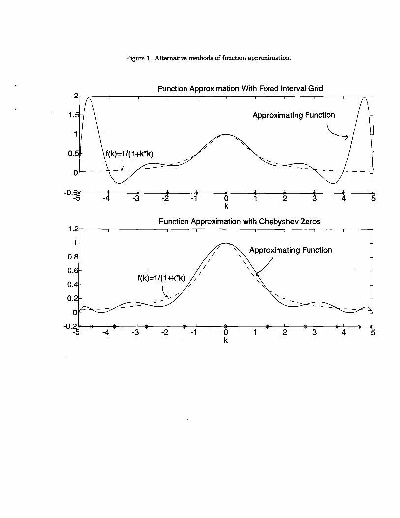
Figure 1. Alternative methods of function approximation.

Function Approximation With Fixed Interval Grid

Approximating Function

Function Approximation with Chebyshev Zeros I 9,

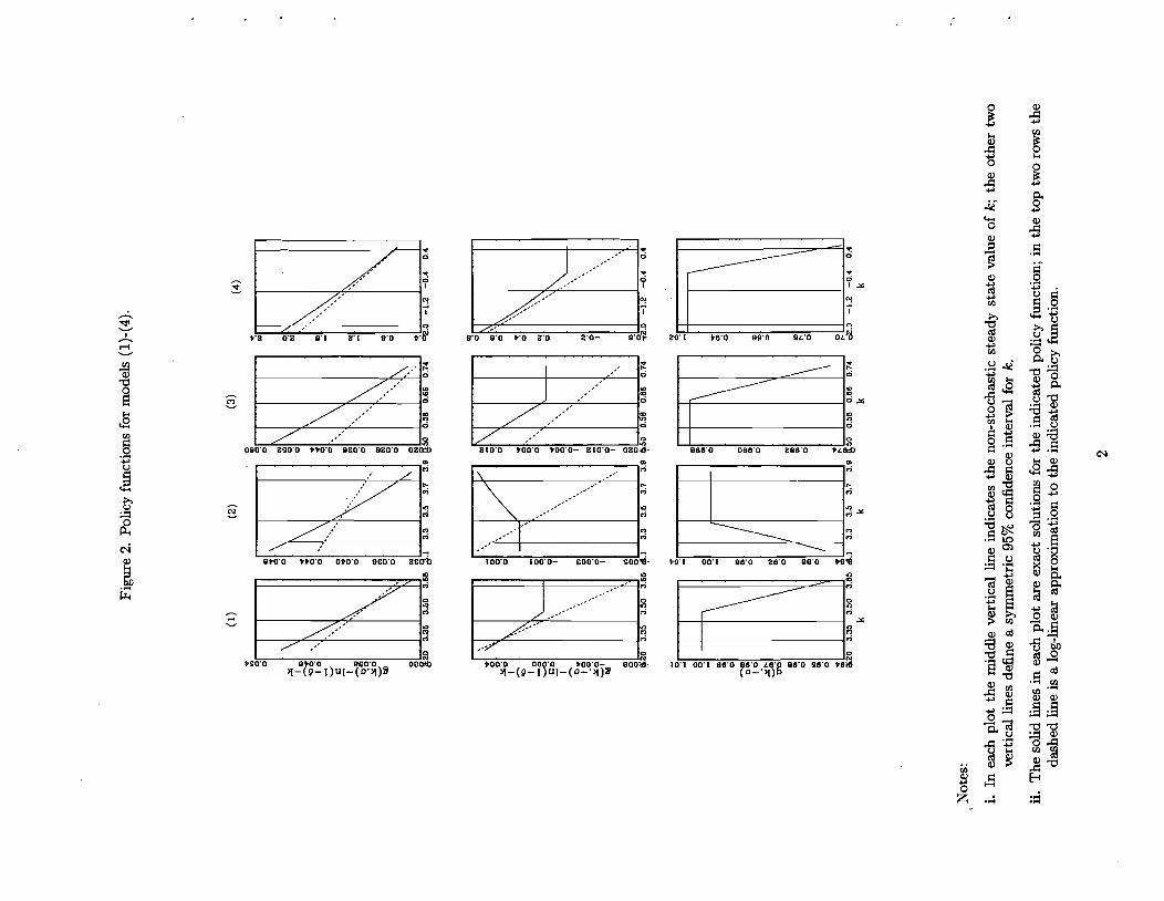
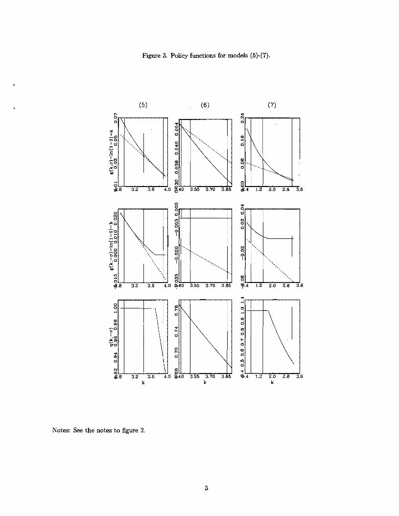
Figure 3. Policy functions for models (5)-(7).

Notes: See the notes to figure 2.

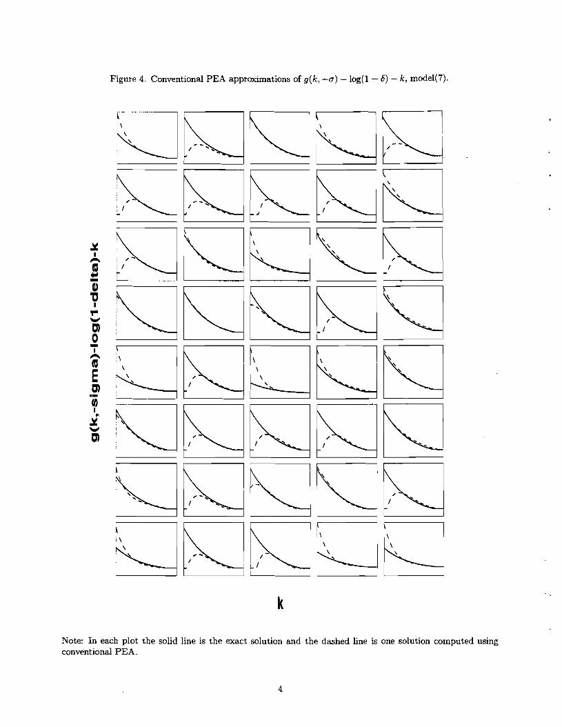
Figure 4. Conventional PEA approximations of g(k, -a) - log(1 - 6) - k, model(7).

Note: In each plot the solid line is the exact solution and the dashed line is one solution computed using conventional PEA.

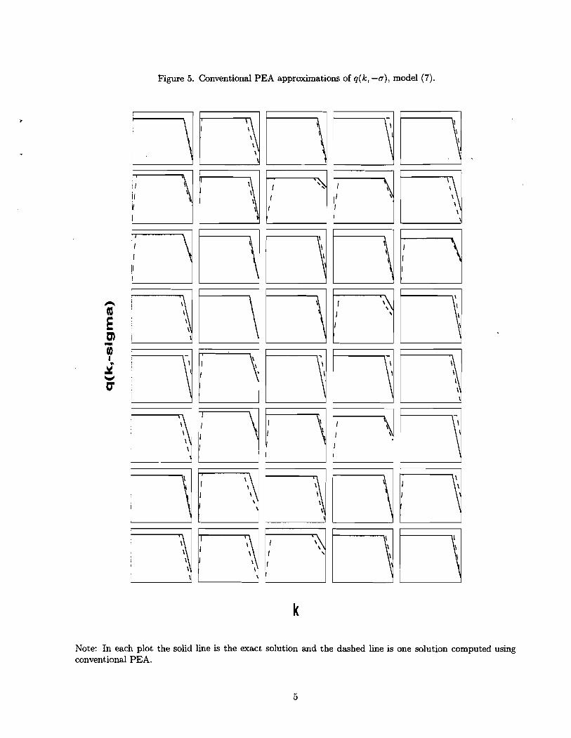
Figure 5. Conventional PEA approximations of q(k , -a), model (7).

Note: In each plot the solid line is the exact solution and the dashed line is one solution computed using conventional PEA.

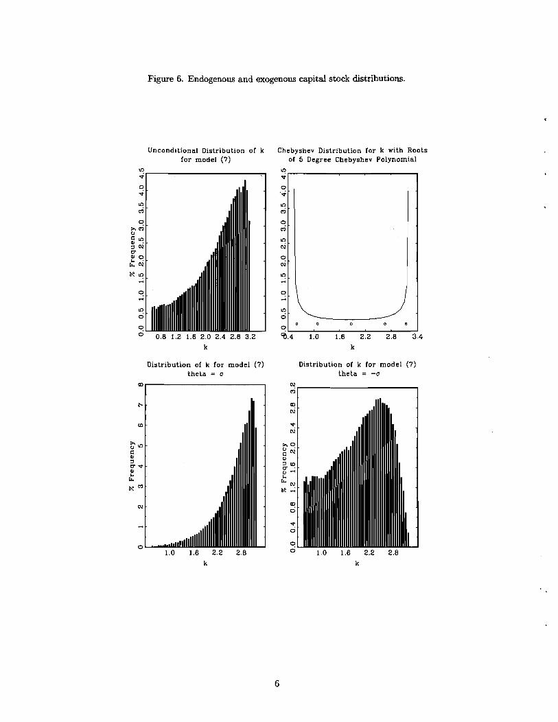
Figure 6. Endogenous and exogenous capital stock distributions.

Unconditional Distribution of k Chebyshev Distribution for k with Roots for model (7) of 5 Degree Chebyshev Polynomial

Distribution of k for model (7) theta = o

Distribution of k for model (7) theta = -0

N,

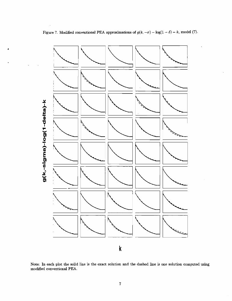
Figure 7. Modified conventional PEA approximations of g(k, -0) - log(1 - 6) - k, model (7).

Note: In each plot the solid line is the exact solution and the dashed line is one solution computed using modified conventional PEA.

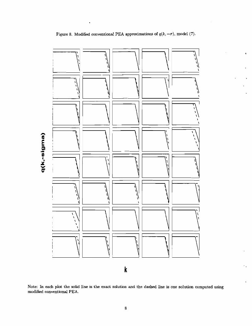
Figure 8. Modified conventional PEA approximations of q(k, -0) , model (7).

Note: In each plot the solid line is the exact solution and the dashed line is one solution computed using modified conventional PEA.

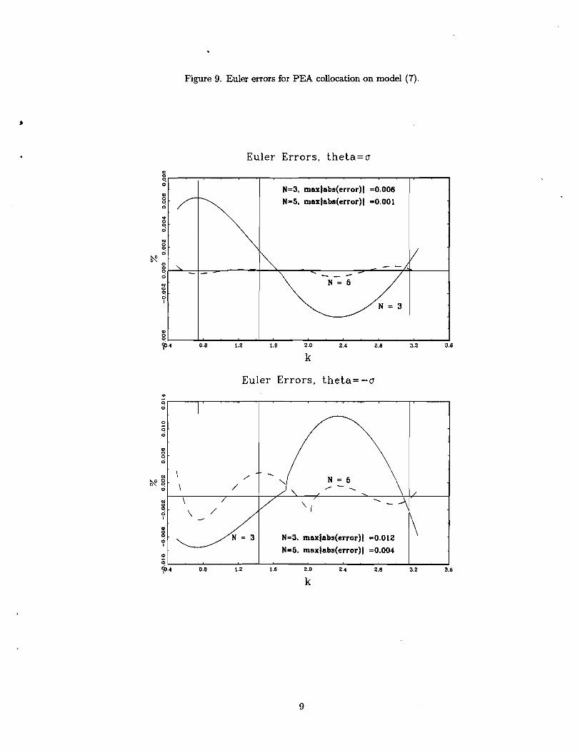
Figure 9. Euler errors for PEA collocation on model (7).

Euler Errors, t he t a=a

Euler Errors, t he t a= -a

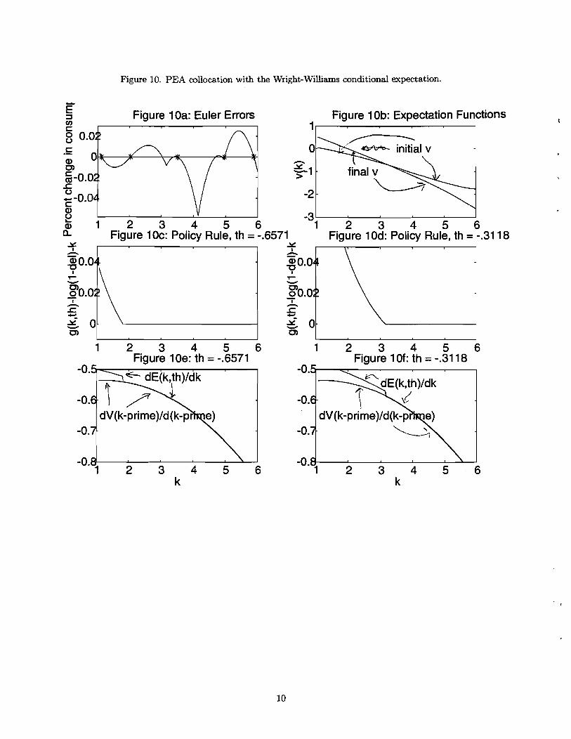
Figure 10. PEA collocation with the Wright-Williams conditional expectation.

EI 3 V)

Figure 10a: Euler Errors Figure 1 0b: Expectation Functions C 8 0.02 C

.- a 0,

5 -0.0i! c 0 - -0.OL1 C

8

ou-,

2 3 4 5 6 & 1 a Figure 10c: Policy Rule, th = -.6571 Figure 10d: Policy Rule, th = -.3118 + h

0,

+ h a 0.04 V 7 w

E?o.o:r - I

F ? 5 0- 0,

1 2 3 4 5 6 1 2 3 4 5 6 Figure 10e: th = -.6571 Figure 1 Of: th = -.3118

-0.5

-0.6-

-0.7-

6 -0.7

2 3 4 5 6 k k