Embed Size (px)
Citation preview
Submitted to the Annals of Statistics
CONSISTENCY OF RANDOM FORESTS
By Erwan Scornet
Sorbonne Universites, UPMC Univ Paris 06, F-75005, Paris, Franceand
By Gerard BiauSorbonne Universites, UPMC Univ Paris 06, F-75005, Paris, France
and
By Jean-Philippe VertMINES ParisTech, PSL-Research University, CBIO-Centre for
Computational Biology, F-77300, Fontainebleau, France& Institut Curie, Paris, F-75248, France
& U900, INSERM, Paris, F-75248, France
Abstract Random forests are a learning algorithm proposed byBreiman (2001) that combines several randomized decision trees andaggregates their predictions by averaging. Despite its wide usage andoutstanding practical performance, little is known about the math-ematical properties of the procedure. This disparity between theoryand practice originates in the difficulty to simultaneously analyzeboth the randomization process and the highly data-dependent treestructure. In the present paper, we take a step forward in forest explo-ration by proving a consistency result for Breiman’s (2001) originalalgorithm in the context of additive regression models. Our analysisalso sheds an interesting light on how random forests can nicely adaptto sparsity.
1. Introduction. Random forests are an ensemble learning method forclassification and regression that constructs a number of randomized deci-sion trees during the training phase and predicts by averaging the results.Since its publication in the seminal paper of Breiman (2001), the proce-dure has become a major data analysis tool, that performs well in practicein comparison with many standard methods. What has greatly contributedto the popularity of forests is the fact that they can be applied to a widerange of prediction problems and have few parameters to tune. Aside frombeing simple to use, the method is generally recognized for its accuracy
MSC 2010 subject classifications: Primary 62G05; secondary 62G20Keywords and phrases: Random forests, randomization, consistency, additive model,
sparsity, dimension reduction
1imsart-aos ver. 2014/10/16 file: article.tex date: May 29, 2015
2 E. SCORNET, G. BIAU AND J.-P. VERT
and its ability to deal with small sample sizes, high-dimensional featurespaces, and complex data structures. The random forest methodology hasbeen successfully involved in many practical problems, including air qual-ity prediction (winning code of the EMC data science global hackathonin 2012, see http://www.kaggle.com/c/dsg-hackathon), chemoinformat-ics (Svetnik et al., 2003), ecology (Prasad et al., 2006; Cutler et al., 2007), 3Dobject recognition (Shotton et al., 2011), and bioinformatics (Dıaz-Uriarteand de Andres, 2006), just to name a few. In addition, many variations onthe original algorithm have been proposed to improve the calculation timewhile maintaining good prediction accuracy (see, e.g., Geurts et al., 2006;Amaratunga et al., 2008). Breiman’s forests have also been extended toquantile estimation (Meinshausen, 2006), survival analysis (Ishwaran et al.,2008), and ranking prediction (Clemencon et al., 2013).
On the theoretical side, the story is less conclusive and, regardless of theirextensive use in practical settings, little is known about the mathematicalproperties of random forests. To date, most studies have concentrated onisolated parts or simplified versions of the procedure. The most celebratedtheoretical result is that of Breiman (2001), which offers an upper boundon the generalization error of forests in terms of correlation and strengthof the individual trees. This was followed by a technical note (Breiman,2004), that focuses on a stylized version of the original algorithm. A criticalstep was subsequently taken by Lin and Jeon (2006), who established lowerbounds for non-adaptive forests (i.e., independent of the training set). Theyalso highlighted an interesting connection between random forests and aparticular class of nearest neighbor predictors that was further worked outby Biau and Devroye (2010). In recent years, various theoretical studies (e.g.,Biau et al., 2008; Ishwaran and Kogalur, 2010; Biau, 2012; Genuer, 2012; Zhuet al., 2012) have been performed, analyzing consistency of simplified models,and moving ever closer to practice. Recent attempts towards narrowing thegap between theory and practice are by Denil et al. (2013), who proves thefirst consistency result for online random forests, and by Wager (2014) andMentch and Hooker (2014) who study the asymptotic sampling distributionof forests.
The difficulty to properly analyze random forests can be explained by theblack-box nature of the procedure, which is actually a subtle combination ofdifferent components. Among the forest essential ingredients, both bagging(Breiman, 1996) and the Classification And Regression Trees (CART)-splitcriterion (Breiman et al., 1984) play a critical role. Bagging (a contraction ofbootstrap-aggregating) is a general aggregation scheme which proceeds bygenerating subsamples from the original data set, constructing a predictor
imsart-aos ver. 2014/10/16 file: article.tex date: May 29, 2015

CONSISTENCY OF RANDOM FORESTS 3
from each resample and deciding by averaging. It is one of the most effectivecomputationally intensive procedures to improve on unstable estimates, es-pecially for large, high-dimensional data sets where finding a good model inone step is impossible because of the complexity and scale of the problem(Buhlmann and Yu, 2002; Kleiner et al., 2014; Wager et al., 2014). As forthe CART-split selection, it is originated from the most influential CARTalgorithm of Breiman et al. (1984), and is used in the construction of theindividual trees to choose the best cuts perpendicular to the axes. At eachnode of each tree, the best cut is selected by optimizing the CART-split cri-terion, based on the notion of Gini impurity (classification) and predictionsquared error (regression).
Yet, while bagging and the CART-splitting scheme play a key role in therandom forest mechanism, both are difficult to analyze, thereby explainingwhy theoretical studies have considered so far simplified versions of the orig-inal procedure. This is often done by simply ignoring the bagging step andby replacing the CART-split selection by a more elementary cut protocol.Besides, in Breiman’s forests, each leaf (that is, a terminal node) of theindividual trees contains a fixed pre-specified number of observations (thisparameter, called nodesize in the R package randomForests, is usuallychosen between 1 and 5). There is also an extra parameter in the algorithmwhich allows to control the total number of leaves (this parameter is calledmaxnode in the R package and has, by default, no effect on the procedure).The combination of these various components makes the algorithm difficultto analyze with rigorous mathematics. As a matter of fact, most authors fo-cus on simplified, data-independent procedures, thus creating a gap betweentheory and practice.
Motivated by the above discussion, we study in the present paper someasymptotic properties of Breiman’s (2001) algorithm in the context of addi-tive regression models. We prove the L2 consistency of random forests, whichgives a first basic theoretical guarantee of efficiency for this algorithm. Up toour knowledge, this is the first consistency result for Breiman’s (2001) orig-inal procedure. Our approach rests upon a detailed analysis of the behaviorof the cells generated by CART-split selection as the sample size grows. Itturns out that a good control of the regression function variation inside eachcell, together with a proper choice of the total number of leaves (Theorem1) or a proper choice of the subsampling rate (Theorem 2) are sufficient toensure the forest consistency in a L2 sense. Also, our analysis shows thatrandom forests can adapt to a sparse framework, when the ambient dimen-sion p is large (independent of n), but only a smaller number of coordinatescarry out information.
imsart-aos ver. 2014/10/16 file: article.tex date: May 29, 2015
4 E. SCORNET, G. BIAU AND J.-P. VERT
The paper is organized as follows. In Section 2, we introduce some nota-tions and describe the random forest method. The main asymptotic resultsare presented in Section 3 and further discussed in Section 4. Section 5 isdevoted to the main proofs, and technical results are gathered in the sup-plemental article (Scornet et al., 2015).
2. Random forests. The general framework is L2 regression estima-tion, in which an input random vector X ∈ [0, 1]p is observed, and the goalis to predict the square integrable random response Y ∈ R by estimatingthe regression function m(x) = E[Y |X = x]. To this aim, we assume givena training sample Dn = (X1, Y1), . . . , (Xn, Yn) of [0, 1]p × R-valued inde-pendent random variables distributed as the independent prototype pair(X, Y ). The objective is to use the data set Dn to construct an estimatemn : [0, 1]p → R of the function m. In this respect, we say that a regressionfunction estimate mn is L2 consistent if E[mn(X)−m(X)]2 → 0 as n→∞(where the expectation is over X and Dn).
A random forest is a predictor consisting of a collection of M random-ized regression trees. For the j-th tree in the family, the predicted value atthe query point x is denoted by mn(x; Θj ,Dn), where Θ1, . . . ,ΘM are inde-pendent random variables, distributed as a generic random variable Θ andindependent of Dn. In practice, this variable is used to resample the trainingset prior to the growing of individual trees and to select the successive can-didate directions for splitting. The trees are combined to form the (finite)forest estimate
mM,n(x; Θ1, . . . ,ΘM ,Dn) =1
M
M∑j=1
mn(x; Θj ,Dn).(1)
Since in practice we can choose M as large as possible, we study in thispaper the property of the infinite forest estimate obtained as the limit of (1)when the number of trees M grows to infinity:
mn(x;Dn) = EΘ [mn(x; Θ,Dn)] ,
where EΘ denotes expectation with respect to the random parameter Θ,conditional on Dn. This operation is justified by the law of large numbers,which asserts that, almost surely, conditional on Dn,
limM→∞
mn,M (x; Θ1, . . . ,ΘM ,Dn) = mn(x;Dn)
(see, e.g., Breiman, 2001; Scornet, 2014, for details). In the sequel, to lightennotation, we will simply write mn(x) instead of mn(x; Dn).
imsart-aos ver. 2014/10/16 file: article.tex date: May 29, 2015
CONSISTENCY OF RANDOM FORESTS 5
Algorithm 1: Breiman’s random forest predicted value at x.
Input: Training set Dn, number of trees M > 0, mtry ∈ {1, . . . , p},an ∈ {1, . . . , n}, tn ∈ {1, . . . , an}, and x ∈ [0, 1]p.
Output: Prediction of the random forest at x.1 for j = 1, . . . ,M do2 Select an points, without replacement, uniformly in Dn.3 Set P0 = {[0, 1]p} the partition associated with the root of the tree.4 For all 1 ≤ ` ≤ an, set P` = ∅.5 Set nnodes = 1 and level = 0.6 while nnodes < tn do7 if Plevel = ∅ then8 level = level + 19 else
10 Let A be the first element in Plevel.11 if A contains exactly one point then12 Plevel ← Plevel\{A}13 Plevel+1 ← Plevel+1 ∪ {A}14 else15 Select uniformly, without replacement, a subset
Mtry ⊂ {1, . . . , p} of cardinality mtry.16 Select the best split in A by optimizing the CART-split
criterion along the coordinates in Mtry (see detailsbelow).
17 Cut the cell A according to the best split. Call AL andAR the two resulting cell.
18 Plevel ← Plevel\{A}19 Plevel+1 ← Plevel+1 ∪ {AL} ∪ {AR}20 nnodes = nnodes + 1
21 end
22 end
23 end24 Compute the predicted value mn(x; Θj ,Dn) at x equal to the
average of the Yi’s falling in the cell of x in partitionPlevel ∪ Plevel+1.
25 end26 Compute the random forest estimate mM,n(x; Θ1, . . . ,ΘM ,Dn) at the
query point x according to (1).
In Breiman’s (2001) original forests, each node of a single tree is associated
imsart-aos ver. 2014/10/16 file: article.tex date: May 29, 2015
6 E. SCORNET, G. BIAU AND J.-P. VERT
with a hyper-rectangular cell. At each step of the tree construction, thecollection of cells forms a partition of [0, 1]p. The root of the tree is [0, 1]p
itself, and each tree is grown as explained in Algorithm 1.This algorithm has three parameters:
1. mtry ∈ {1, . . . , p}, which is the number of pre-selected directions forsplitting;
2. an ∈ {1, . . . , n}, which is the number of sampled data points in eachtree;
3. tn ∈ {1, . . . , an}, which is the number of leaves in each tree.
By default, in the original procedure, the parameter mtry is set to p/3, anis set to n (resampling is done with replacement), and tn = an. However, inour approach, resampling is done without replacement and the parametersan and tn can be different from their default values.
In a word, the algorithm works by growing M different trees as follows.For each tree, an data points are drawn at random without replacementfrom the original data set; then, at each cell of every tree, a split is chosenby maximizing the CART-criterion (see below); finally, the construction ofevery tree is stopped when the total number of cells in the tree reaches thevalue tn (therefore, each cell contains exactly one point in the case tn = an).
We note that the resampling step in Algorithm 1 (line 2) is done bychoosing an out of n points (with an ≤ n) without replacement. This isslightly different from the original algorithm, where resampling is done bybootstrapping, that is by choosing n out of n data points with replacement.
Selecting the points “without replacement” instead of “with replacement”is harmless—in fact, it is just a means to avoid mathematical difficultiesinduced by the bootstrap (see, e.g., Bradley, 1982; Politis et al., 1999).
On the other hand, letting the parameters an and tn depend upon n offersseveral degrees of freedom which opens the route for establishing consistencyof the method. To be precise, we will study in Section 3 the random forestalgorithm in two different regimes. The first regime is when tn < an, whichmeans that trees are not fully developed. In that case, a proper tuning oftn ensures the forest’s consistency (Theorem 1). The second regime occurswhen tn = an, i.e. when trees are fully grown. In that case, consistencyresults from an appropriate choice of the subsample rate an/n (Theorem 2).
So far, we have not made explicit the CART-split criterion used in Al-gorithm 1. To properly define it, we let A be a generic cell and Nn(A) bethe number of data points falling in A. A cut in A is a pair (j, z), where jis a dimension in {1, . . . , p} and z is the position of the cut along the j-thcoordinate, within the limits of A. We let CA be the set of all such possible
imsart-aos ver. 2014/10/16 file: article.tex date: May 29, 2015
CONSISTENCY OF RANDOM FORESTS 7
cuts in A. Then, with the notation Xi = (X(1)i , . . . ,X
(p)i ), for any (j, z) ∈ CA,
the CART-split criterion (Breiman et al., 1984) takes the form
Ln(j, z) =1
Nn(A)
n∑i=1
(Yi − YA)21Xi∈A
− 1
Nn(A)
n∑i=1
(Yi − YAL1X(j)i <z
− YAR1X(j)i ≥z
)21Xi∈A,(2)
where AL = {x ∈ A : x(j) < z}, AR = {x ∈ A : x(j) ≥ z}, and YA (resp.,YAL , YAR) is the average of the Yi’s belonging to A (resp., AL, AR), with theconvention 0/0 = 0. At each cell A, the best cut (j?n, z
?n) is finally selected
by maximizing Ln(j, z) over Mtry and CA, that is
(j?n, z?n) ∈ arg max
j∈Mtry
(j,z)∈CA
Ln(j, z).
To remove ties in the argmax, the best cut is always performed along thebest cut direction j?n, at the middle of two consecutive data points.
3. Main results. We consider an additive regression model satisfyingthe following properties:
(H1) The response Y follows
Y =
p∑j=1
mj(X(j)) + ε,
where X = (X(1), . . . ,X(p)) is uniformly distributed over [0, 1]p, ε is anindependent centered Gaussian noise with finite variance σ2 > 0, and eachcomponent mj is continuous.
Additive regression models, which extend linear models, were popularizedby Stone (1985) and Hastie and Tibshirani (1986). These models, which de-compose the regression function as a sum of univariate functions, are flexibleand easy to interpret. They are acknowledged for providing a good trade-off between model complexity and calculation time, and were accordinglyextensively studied for the last thirty years. Additive models also play animportant role in the context of high-dimensional data analysis and sparsemodelling, where they are successfully involved in procedures such as theLasso and various aggregation schemes (for an overview, see, e.g., Hastieet al., 2009). Although random forests fall in the family of non parametric
imsart-aos ver. 2014/10/16 file: article.tex date: May 29, 2015
8 E. SCORNET, G. BIAU AND J.-P. VERT
procedures, it turns out that the analysis of their properties is facilitatedwithin the framework of additive models.
Our first result assumes that the total number of leaves tn in each treetends to infinity slower than the number of selected data points an.
Theorem 1. Assume that (H1) is satisfied. Then, provided an → ∞,tn →∞ and tn(log an)9/an → 0, random forests are consistent, i.e.,
limn→∞
E [mn(X)−m(X)]2 = 0.
Noteworthy, Theorem 1 still holds with an = n. In that case, the subsam-pling step plays no role in the consistency of the method. Indeed, controllingthe depth of the trees via the parameter tn is sufficient to bound the foresterror. We note in passing that an easy adaptation of Theorem 1 shows thatthe CART algorithm is consistent under the same assumptions.
The term (log an)9 originates from the Gaussian noise and allows to con-trol the noise tail. In the easier situation where the Gaussian noise is replacedby a bounded random variable, it is easy to see that the term (log an)9 turnsinto log an, a term which accounts for the complexity of the tree partition.
Let us now examine the forest behavior in the second regime, where tn =an (i.e., trees are fully grown) and, as before, subsampling is done at therate an/n. The analysis of this regime turns out to be more complicated,and rests upon assumption (H2) below. We denote by Zi = 1
XΘ↔Xi
the
indicator that Xi falls in the same cell as X in the random tree designedwith Dn and the random parameter Θ. Similarly, we let Z ′j = 1
XΘ′↔Xj
, where
Θ′ is an independent copy of Θ. Accordingly, we define
ψi,j(Yi, Yj) = E[ZiZ
′j
∣∣X,Θ,Θ′,X1, . . . ,Xn, Yi, Yj
]and ψi,j = E
[ZiZ
′j
∣∣X,Θ,Θ′,X1, . . . ,Xn
].
Finally, for any random variables W1, W2, Z, we denote by Corr(W1, W2|Z)the conditional correlation coefficient (whenever it exists).
(H2) Let Zi,j = (Zi, Z′j). Then, one of the following two conditions holds:
(H2.1) One has
limn→∞
(log an)2p−2(log n)2E
[maxi,ji 6=j
|ψi,j(Yi, Yj)− ψi,j |
]2
= 0.
imsart-aos ver. 2014/10/16 file: article.tex date: May 29, 2015
CONSISTENCY OF RANDOM FORESTS 9
(H2.2) There exist a constant C > 0 and a sequence (γn)n → 0 suchthat, almost surely,
max`1,`2=0,1
|Corr(Yi −m(Xi),1Zi,j=(`1,`2)|Xi,Xj , Yj)|P1/2
[Zi,j = (`1, `2)|Xi,Xj , Yj
] ≤ γn,
and
max`1=0,1
|Corr((Yi −m(Xi))
2,1Zi=`1 |Xi
)|
P1/2[Zi = `1|Xi
] ≤ C.
Despite their technical aspect, statements (H2.1) and (H2.2) have sim-ple interpretations. To understand the meaning of (H2.1), let us replace theGaussian noise by a bounded random variable. A close inspection of Lemma4 shows that (H2.1) may be simply replaced by
limn→∞
E
[maxi,ji 6=j
|ψi,j(Yi, Yj)− ψi,j |
]2
= 0.
Therefore, (H2.1) means that the influence of two Y-values on the proba-bility of connection of two couples of random points tends to zero as n→∞.
As for assumption (H2.2), it holds whenever the correlation between thenoise and the probability of connection of two couples of random pointsvanishes fast enough, as n → ∞. Note that, in the simple case where thepartition is independent of the Yi’s, the correlations in (H2.2) are zero, sothat (H2) is trivially satisfied. It is also verified in the noiseless case, thatis, when Y = m(X). However, in the most general context, the partitionsstrongly depend on the whole sample Dn and, unfortunately, we do not knowwhether (H2) is satisfied or not.
Theorem 2. Assume that (H1) and (H2) are satisfied and let tn = an.Then, provided an →∞ and an log n/n→ 0, random forests are consistent,i.e.,
limn→∞
E [mn(X)−m(X)]2 = 0.
Up to our knowledge, apart from the fact that bootstrapping is replacedby subsampling, Theorem 1 and Theorem 2 are the first consistency resultsfor Breiman’s (2001) forests. Indeed, most models studied so far are designedindependently of Dn and are, consequently, an unrealistic representation ofthe true procedure. In fact, understanding Breiman’s random forest behaviordeserves a more involved mathematical treatment. Section 4 below offers athorough description of the various mathematical forces in action.
imsart-aos ver. 2014/10/16 file: article.tex date: May 29, 2015
10 E. SCORNET, G. BIAU AND J.-P. VERT
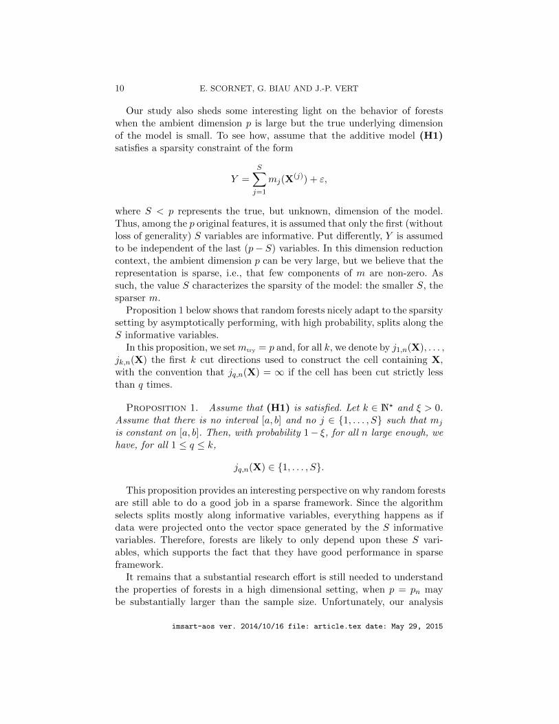
Our study also sheds some interesting light on the behavior of forestswhen the ambient dimension p is large but the true underlying dimensionof the model is small. To see how, assume that the additive model (H1)satisfies a sparsity constraint of the form
Y =S∑j=1
mj(X(j)) + ε,
where S < p represents the true, but unknown, dimension of the model.Thus, among the p original features, it is assumed that only the first (withoutloss of generality) S variables are informative. Put differently, Y is assumedto be independent of the last (p− S) variables. In this dimension reductioncontext, the ambient dimension p can be very large, but we believe that therepresentation is sparse, i.e., that few components of m are non-zero. Assuch, the value S characterizes the sparsity of the model: the smaller S, thesparser m.
Proposition 1 below shows that random forests nicely adapt to the sparsitysetting by asymptotically performing, with high probability, splits along theS informative variables.
In this proposition, we setmtry = p and, for all k, we denote by j1,n(X), . . . ,jk,n(X) the first k cut directions used to construct the cell containing X,with the convention that jq,n(X) = ∞ if the cell has been cut strictly lessthan q times.
Proposition 1. Assume that (H1) is satisfied. Let k ∈ N? and ξ > 0.Assume that there is no interval [a, b] and no j ∈ {1, . . . , S} such that mj
is constant on [a, b]. Then, with probability 1− ξ, for all n large enough, wehave, for all 1 ≤ q ≤ k,
jq,n(X) ∈ {1, . . . , S}.
This proposition provides an interesting perspective on why random forestsare still able to do a good job in a sparse framework. Since the algorithmselects splits mostly along informative variables, everything happens as ifdata were projected onto the vector space generated by the S informativevariables. Therefore, forests are likely to only depend upon these S vari-ables, which supports the fact that they have good performance in sparseframework.
It remains that a substantial research effort is still needed to understandthe properties of forests in a high dimensional setting, when p = pn maybe substantially larger than the sample size. Unfortunately, our analysis
imsart-aos ver. 2014/10/16 file: article.tex date: May 29, 2015

CONSISTENCY OF RANDOM FORESTS 11
does not carry over to this context. In particular, if high-dimensionality ismodelled by letting pn →∞, then assumption (H2.1) may be too restrictivesince the term (log an)2p−2 will diverge at a fast rate.
4. Discussion. One of the main difficulties in assessing the mathemat-ical properties of Breiman’s (2001) forests is that the construction processof the individual trees strongly depends on both the Xi’s and the Yi’s. Forpartitions that are independent of the Yi’s, consistency can be shown byrelatively simple means via Stone’s (1977) theorem for local averaging esti-mates (see also Gyorfi et al., 2002, Chapter 6). However, our partitions andtrees depend upon the Y -values in the data. This makes things complicated,but mathematically interesting too. Thus, logically, the proof of Theorem2 starts with an adaptation of Stone’s (1977) theorem tailored for randomforests, whereas the proof of Theorem 1 is based on consistency results ofdata-dependent partitions developed by Nobel (1996).
Both theorems rely on Proposition 2 below which stresses an importantfeature of the random forest mechanism. It states that the variation of theregression function m within a cell of a random tree is small provided nis large enough. To this aim, we define, for any cell A, the variation of mwithin A as
∆(m,A) = supx,x′∈A
|m(x)−m(x′)|.
Furthermore, we denote by An(X,Θ) the cell of a tree built with randomparameter Θ that contains the point X.
Proposition 2. Assume that (H1) holds. Then, for all ρ, ξ > 0, thereexists N ∈ N? such that, for all n > N ,
P [∆(m,An(X,Θ)) ≤ ξ] ≥ 1− ρ.
It should be noted that in the standard, Y -independent analysis of par-titioning regression function estimates, the variance is controlled by lettingthe diameters of the tree cells tend to zero in probability. Instead of such ageometrical assumption, Proposition 2 ensures that the variation of m in-side a cell is small, thereby forcing the approximation error of the forest toasymptotically approach zero.
While Proposition 2 offers a good control of the approximation error ofthe forest in both regimes, a separated analysis is required for the estimationerror. In regime 1 (Theorem 1), the parameter tn allows to control the struc-ture of the tree. This is in line with standard tree consistency approaches
imsart-aos ver. 2014/10/16 file: article.tex date: May 29, 2015

12 E. SCORNET, G. BIAU AND J.-P. VERT
(see, e.g., Chapter 20 in Devroye et al., 1996). Things are different for thesecond regime (Theorem 2), in which individual trees are fully grown. Inthat case, the estimation error is controlled by forcing the subsampling ratean/n to be o(1/ log n), which is a more unusual requirement and deservessome remarks.
At first, we note that the log n term in Theorem 2 is used to controlthe Gaussian noise ε. Thus, if the noise is assumed to be a bounded ran-dom variable, then the logn term disappears, and the condition reduces toan/n → 0. The requirement an log n/n → 0 guarantees that every singleobservation (Xi, Yi) is used in the tree construction with a probability thatbecomes small with n. It also implies that the query point x is not connectedto the same data point in a high proportion of trees. If not, the predictedvalue at x would be too much influenced by one single pair (Xi, Yi), mak-ing the forest inconsistent. In fact, the proof of Theorem 2 reveals that theestimation error of a forest estimate is small as soon as the maximum prob-ability of connection between the query point and all observations is small.Thus, the assumption on the subsampling rate is just a convenient way tocontrol these probabilities, by ensuring that partitions are dissimilar enough(i.e. by ensuring that x is connected with many data points through the for-est). This idea of diversity among trees was introduced by Breiman (2001),but is generally difficult to analyse. In our approach, the subsampling is thekey component for imposing tree diversity.
Theorem 2 comes at the price of assumption (H2), for which we do notknow if it is valid in all generality. On the other hand, Theorem 2, whichmimics almost perfectly the algorithm used in practice, is an importantstep towards understanding Breiman’s random forests. Contrary to mostprevious works, Theorem 2 assumes that there is only one observation perleaf of each individual tree. This implies that the single trees are eventuallynot consistent, since standard conditions for tree consistency require that thenumber of observations in the terminal nodes tends to infinity as n grows(see, e.g., Devroye et al., 1996; Gyorfi et al., 2002). Thus, the random forestalgorithm aggregates rough individual tree predictors to build a provablyconsistent general architecture.
It is also interesting to note that our results (in particular Lemma 3)cannot be directly extended to establish the pointwise consistency of randomforests, that is, for almost all x ∈ [0, 1]d,
limn→∞
E[mn(x)−m(x)
]2= 0.
Fixing x ∈ [0, 1]d, the difficulty results from the fact that we do not have acontrol on the diameter of the cell An(x,Θ), whereas, since the cells form
imsart-aos ver. 2014/10/16 file: article.tex date: May 29, 2015

CONSISTENCY OF RANDOM FORESTS 13
a partition of [0, 1]d, we have a global control on their diameters. Thus,as highlighted by Wager (2014), random forests can be inconsistent at somefixed point x ∈ [0, 1]d, particularly near the edges, while being L2 consistent.
Let us finally mention that all results can be extended to the case where εis a heteroscedastic and sub-Gaussian noise, with for all x ∈ [0, 1]d, V[ε|X =x] ≤ σ′2, for some constant σ′2. All proofs can be readily extended to matchthis context, at the price of easy technical adaptations.
5. Proof of Theorem 1 and Theorem 2. For the sake of clarity,proofs of the intermediary results are gathered in in the supplemental article(Scornet et al., 2015). We start with some notations.
5.1. Notations. In the sequel, to clarify the notations, we will sometimeswrite d = (d(1), d(2)) to represent a cut (j, z).
Recall that, for any cell A, CA is the set of all possible cuts in A. Thus,with this notation, C[0,1]p is just the set of all possible cuts at the root of the
tree, that is, all possible choices d = (d(1), d(2)) with d(1) ∈ {1, . . . , p} andd(2) ∈ [0, 1].
More generally, for any x ∈ [0, 1]p, we call Ak(x) the collection of allpossible k ≥ 1 consecutive cuts used to build the cell containing x. Sucha cell is obtained after a sequence of cuts dk = (d1, . . . , dk), where thedependency of dk upon x is understood. Accordingly, for any dk ∈ Ak(x),we let A(x,dk) be the cell containing x built with the particular k-tuple ofcuts dk. The proximity between two elements dk and d′k in Ak(x) will bemeasured via
‖dk − d′k‖∞ = sup1≤j≤k
max(|d(1)j − d
′(1)j |, |d
(2)j − d
′(2)j |).
Accordingly, the distance d∞ between dk ∈ Ak(x) and any A ⊂ Ak(x) is
d∞(dk,A) = infz∈A‖dk − z‖∞.
Remember that An(X,Θ) denotes the cell of a tree containing X anddesigned with random parameter Θ. Similarly, Ak,n(X,Θ) is the same cellbut where only the first k cuts are performed (k ∈ N? is a parameter to bechosen later). We also denote by dk,n(X,Θ) = (d1,n(X,Θ), . . . , dk,n(X,Θ))the k cuts used to construct the cell Ak,n(X,Θ).
Recall that, for any cell A, the empirical criterion used to split A in therandom forest algorithm is defined in (2). For any cut (j, z) ∈ CA, we denote
imsart-aos ver. 2014/10/16 file: article.tex date: May 29, 2015
14 E. SCORNET, G. BIAU AND J.-P. VERT
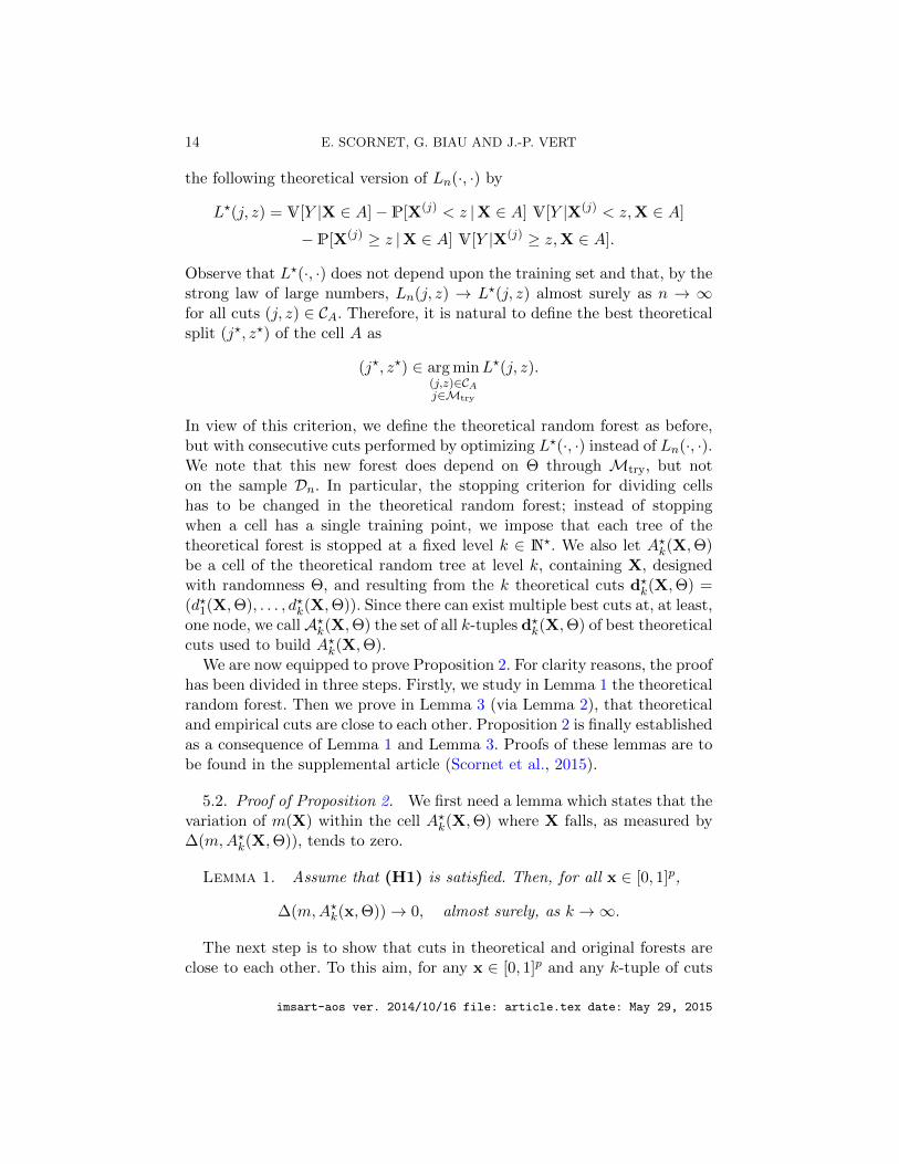
the following theoretical version of Ln(·, ·) by
L?(j, z) = V[Y |X ∈ A]− P[X(j) < z |X ∈ A] V[Y |X(j) < z,X ∈ A]
− P[X(j) ≥ z |X ∈ A] V[Y |X(j) ≥ z,X ∈ A].
Observe that L?(·, ·) does not depend upon the training set and that, by thestrong law of large numbers, Ln(j, z) → L?(j, z) almost surely as n → ∞for all cuts (j, z) ∈ CA. Therefore, it is natural to define the best theoreticalsplit (j?, z?) of the cell A as
(j?, z?) ∈ arg min(j,z)∈CAj∈Mtry
L?(j, z).
In view of this criterion, we define the theoretical random forest as before,but with consecutive cuts performed by optimizing L?(·, ·) instead of Ln(·, ·).We note that this new forest does depend on Θ through Mtry, but noton the sample Dn. In particular, the stopping criterion for dividing cellshas to be changed in the theoretical random forest; instead of stoppingwhen a cell has a single training point, we impose that each tree of thetheoretical forest is stopped at a fixed level k ∈ N?. We also let A?k(X,Θ)be a cell of the theoretical random tree at level k, containing X, designedwith randomness Θ, and resulting from the k theoretical cuts d?k(X,Θ) =(d?1(X,Θ), . . . , d?k(X,Θ)). Since there can exist multiple best cuts at, at least,one node, we callA?k(X,Θ) the set of all k-tuples d?k(X,Θ) of best theoreticalcuts used to build A?k(X,Θ).
We are now equipped to prove Proposition 2. For clarity reasons, the proofhas been divided in three steps. Firstly, we study in Lemma 1 the theoreticalrandom forest. Then we prove in Lemma 3 (via Lemma 2), that theoreticaland empirical cuts are close to each other. Proposition 2 is finally establishedas a consequence of Lemma 1 and Lemma 3. Proofs of these lemmas are tobe found in the supplemental article (Scornet et al., 2015).
5.2. Proof of Proposition 2. We first need a lemma which states that thevariation of m(X) within the cell A?k(X,Θ) where X falls, as measured by∆(m,A?k(X,Θ)), tends to zero.
Lemma 1. Assume that (H1) is satisfied. Then, for all x ∈ [0, 1]p,
∆(m,A?k(x,Θ))→ 0, almost surely, as k →∞.
The next step is to show that cuts in theoretical and original forests areclose to each other. To this aim, for any x ∈ [0, 1]p and any k-tuple of cuts
imsart-aos ver. 2014/10/16 file: article.tex date: May 29, 2015
CONSISTENCY OF RANDOM FORESTS 15
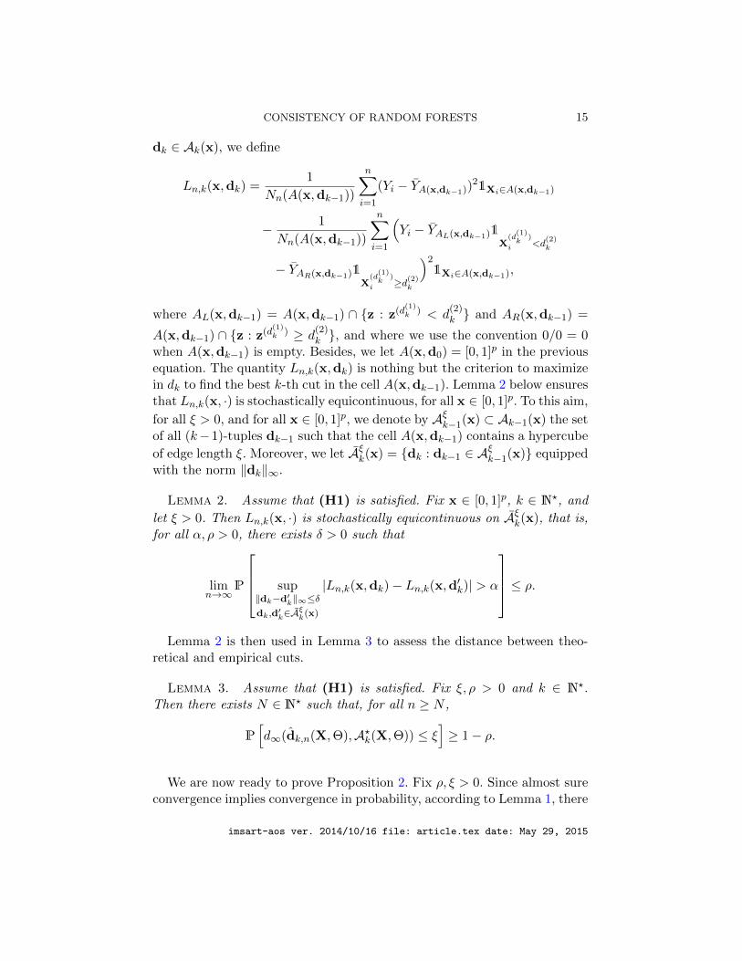
dk ∈ Ak(x), we define
Ln,k(x,dk) =1
Nn(A(x,dk−1))
n∑i=1
(Yi − YA(x,dk−1))21Xi∈A(x,dk−1)
− 1
Nn(A(x,dk−1))
n∑i=1
(Yi − YAL(x,dk−1)1
X(d
(1)k
)
i <d(2)k
− YAR(x,dk−1)1X
(d(1)k
)
i ≥d(2)k
)21Xi∈A(x,dk−1),
where AL(x,dk−1) = A(x,dk−1) ∩ {z : z(d(1)k ) < d
(2)k } and AR(x,dk−1) =
A(x,dk−1) ∩ {z : z(d(1)k ) ≥ d
(2)k }, and where we use the convention 0/0 = 0
when A(x,dk−1) is empty. Besides, we let A(x,d0) = [0, 1]p in the previousequation. The quantity Ln,k(x,dk) is nothing but the criterion to maximizein dk to find the best k-th cut in the cell A(x,dk−1). Lemma 2 below ensuresthat Ln,k(x, ·) is stochastically equicontinuous, for all x ∈ [0, 1]p. To this aim,
for all ξ > 0, and for all x ∈ [0, 1]p, we denote by Aξk−1(x) ⊂ Ak−1(x) the setof all (k−1)-tuples dk−1 such that the cell A(x,dk−1) contains a hypercube
of edge length ξ. Moreover, we let Aξk(x) = {dk : dk−1 ∈ Aξk−1(x)} equippedwith the norm ‖dk‖∞.
Lemma 2. Assume that (H1) is satisfied. Fix x ∈ [0, 1]p, k ∈ N?, and
let ξ > 0. Then Ln,k(x, ·) is stochastically equicontinuous on Aξk(x), that is,for all α, ρ > 0, there exists δ > 0 such that
limn→∞
P
sup‖dk−d′k‖∞≤δdk,d
′k∈A
ξk(x)
|Ln,k(x,dk)− Ln,k(x,d′k)| > α
≤ ρ.Lemma 2 is then used in Lemma 3 to assess the distance between theo-
retical and empirical cuts.
Lemma 3. Assume that (H1) is satisfied. Fix ξ, ρ > 0 and k ∈ N?.Then there exists N ∈ N? such that, for all n ≥ N ,
P[d∞(dk,n(X,Θ),A?k(X,Θ)) ≤ ξ
]≥ 1− ρ.
We are now ready to prove Proposition 2. Fix ρ, ξ > 0. Since almost sureconvergence implies convergence in probability, according to Lemma 1, there
imsart-aos ver. 2014/10/16 file: article.tex date: May 29, 2015
16 E. SCORNET, G. BIAU AND J.-P. VERT
exists k0 ∈ N? such that
P[∆(m,A?k0
(X,Θ)) ≤ ξ]≥ 1− ρ.(3)
By Lemma 3, for all ξ1 > 0, there exists N ∈ N? such that, for all n ≥ N ,
P[d∞(dk0,n(X,Θ),A?k0
(X,Θ)) ≤ ξ1
]≥ 1− ρ.(4)
Since m is uniformly continuous, we can choose ξ1 sufficiently small suchthat, for all x ∈ [0, 1]p, for all dk0 ,d
′k0
satisfying d∞(dk0 ,d′k0
) ≤ ξ1, we have∣∣∆(m,A(x,dk0))−∆(m,A(x,d′k0))∣∣ ≤ ξ.(5)
Thus, combining inequalities (4) and (5), we obtain
P[ ∣∣∆(m,Ak0,n(X,Θ))−∆(m,A?k0
(X,Θ))∣∣ ≤ ξ] ≥ 1− ρ.(6)
Using the fact that ∆(m,A) ≤ ∆(m,A′) whenever A ⊂ A′, we deduce from(3) and (6) that, for all n ≥ N ,
P [∆(m,An(X,Θ)) ≤ 2ξ] ≥ 1− 2ρ.
This concludes the proof of Proposition 2.
5.3. Proof of Theorem 1. We still need some additional notations. Thepartition obtained with the random variable Θ and the data set Dn is de-noted by Pn(Dn,Θ), which we abbreviate as Pn(Θ). We let
Πn(Θ) = {P((x1, y1), . . . , (xn, yn),Θ) : (xi, yi) ∈ [0, 1]d ×R}
be the family of all achievable partitions with random parameter Θ. Accord-ingly, we let
M(Πn(Θ)) = max {Card(P) : P ∈ Πn(Θ)}
be the maximal number of terminal nodes among all partitions in Πn(Θ).Given a set zn1 = {z1, . . . , zn} ⊂ [0, 1]d, Γ(zn1 ,Πn(Θ)) denotes the number ofdistinct partitions of zn1 induced by elements of Πn(Θ), that is, the numberof different partitions {zn1 ∩A : A ∈ P} of zn1 , for P ∈ Πn(Θ). Consequently,the partitioning number Γn(Πn(Θ)) is defined by
Γn(Πn(Θ)) = max{
Γ(zn1 ,Πn(Θ)) : z1, . . . , zn ∈ [0, 1]d}.
imsart-aos ver. 2014/10/16 file: article.tex date: May 29, 2015
CONSISTENCY OF RANDOM FORESTS 17
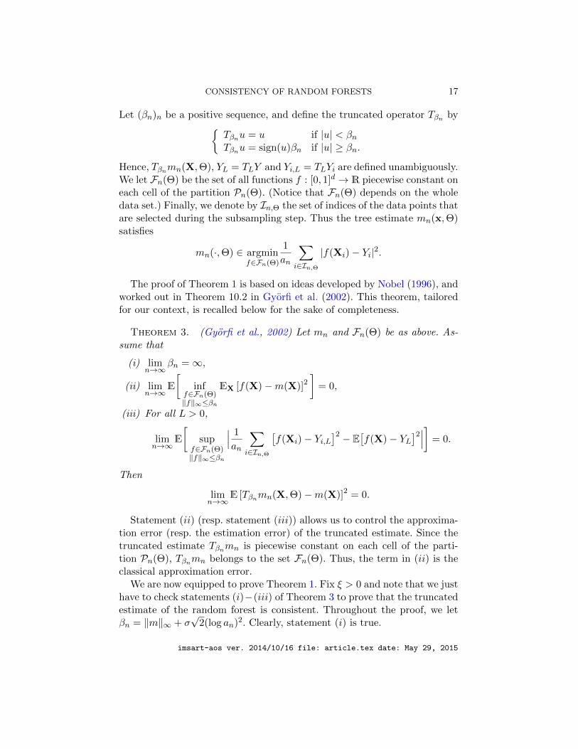
Let (βn)n be a positive sequence, and define the truncated operator Tβn by{Tβnu = u if |u| < βnTβnu = sign(u)βn if |u| ≥ βn.
Hence, Tβnmn(X,Θ), YL = TLY and Yi,L = TLYi are defined unambiguously.We let Fn(Θ) be the set of all functions f : [0, 1]d → R piecewise constant oneach cell of the partition Pn(Θ). (Notice that Fn(Θ) depends on the wholedata set.) Finally, we denote by In,Θ the set of indices of the data points thatare selected during the subsampling step. Thus the tree estimate mn(x,Θ)satisfies
mn(·,Θ) ∈ argminf∈Fn(Θ)
1
an
∑i∈In,Θ
|f(Xi)− Yi|2.
The proof of Theorem 1 is based on ideas developed by Nobel (1996), andworked out in Theorem 10.2 in Gyorfi et al. (2002). This theorem, tailoredfor our context, is recalled below for the sake of completeness.
Theorem 3. (Gyorfi et al., 2002) Let mn and Fn(Θ) be as above. As-sume that
(i) limn→∞
βn =∞,
(ii) limn→∞
E
[inf
f∈Fn(Θ)‖f‖∞≤βn
EX [f(X)−m(X)]2]
= 0,
(iii) For all L > 0,
limn→∞
E
[sup
f∈Fn(Θ)‖f‖∞≤βn
∣∣∣ 1
an
∑i∈In,Θ
[f(Xi)− Yi,L
]2 − E[f(X)− YL
]2∣∣∣] = 0.
Then
limn→∞
E [Tβnmn(X,Θ)−m(X)]2 = 0.
Statement (ii) (resp. statement (iii)) allows us to control the approxima-tion error (resp. the estimation error) of the truncated estimate. Since thetruncated estimate Tβnmn is piecewise constant on each cell of the parti-tion Pn(Θ), Tβnmn belongs to the set Fn(Θ). Thus, the term in (ii) is theclassical approximation error.
We are now equipped to prove Theorem 1. Fix ξ > 0 and note that we justhave to check statements (i)−(iii) of Theorem 3 to prove that the truncatedestimate of the random forest is consistent. Throughout the proof, we letβn = ‖m‖∞ + σ
√2(log an)2. Clearly, statement (i) is true.
imsart-aos ver. 2014/10/16 file: article.tex date: May 29, 2015
18 E. SCORNET, G. BIAU AND J.-P. VERT
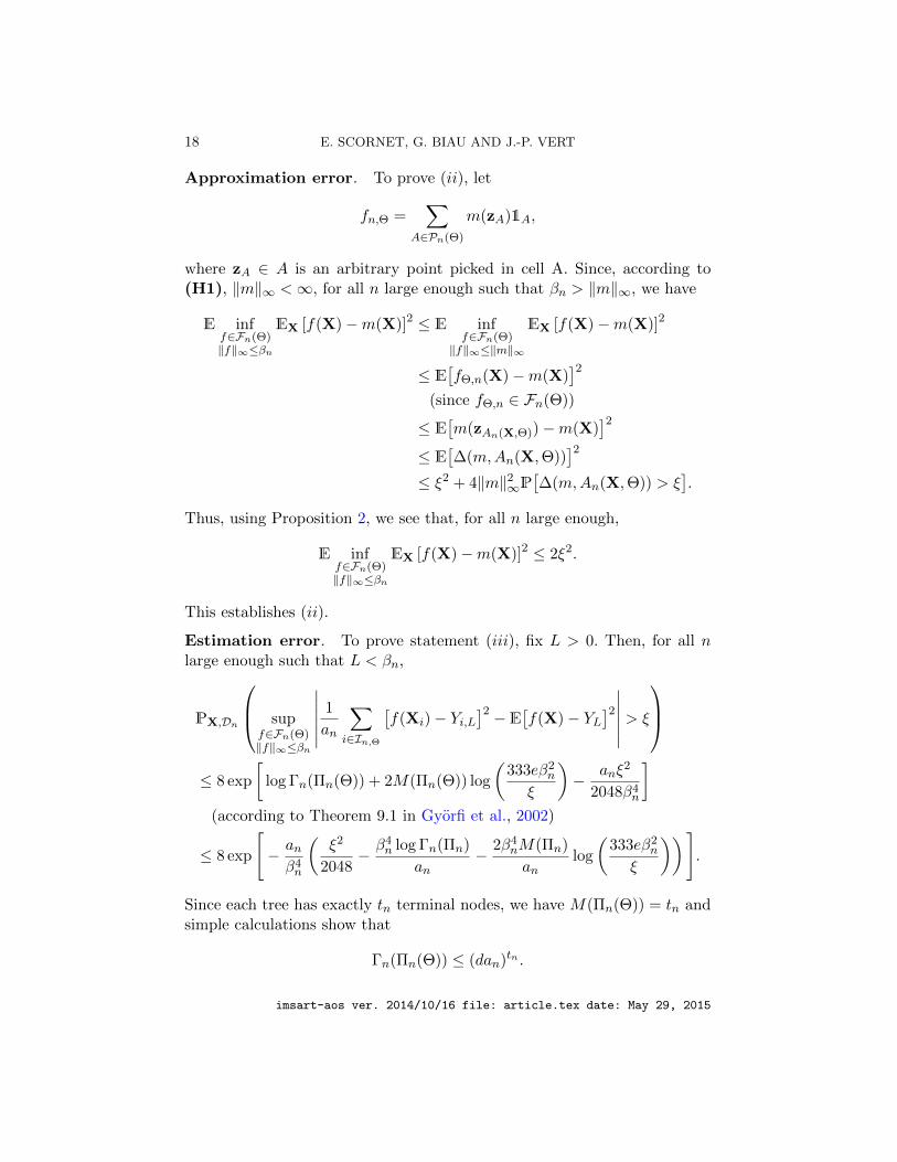
Approximation error. To prove (ii), let
fn,Θ =∑
A∈Pn(Θ)
m(zA)1A,
where zA ∈ A is an arbitrary point picked in cell A. Since, according to(H1), ‖m‖∞ <∞, for all n large enough such that βn > ‖m‖∞, we have
E inff∈Fn(Θ)‖f‖∞≤βn
EX [f(X)−m(X)]2 ≤ E inff∈Fn(Θ)‖f‖∞≤‖m‖∞
EX [f(X)−m(X)]2
≤ E[fΘ,n(X)−m(X)
]2(since fΘ,n ∈ Fn(Θ))
≤ E[m(zAn(X,Θ))−m(X)
]2≤ E
[∆(m,An(X,Θ))
]2≤ ξ2 + 4‖m‖2∞P
[∆(m,An(X,Θ)) > ξ
].
Thus, using Proposition 2, we see that, for all n large enough,
E inff∈Fn(Θ)‖f‖∞≤βn
EX [f(X)−m(X)]2 ≤ 2ξ2.
This establishes (ii).
Estimation error. To prove statement (iii), fix L > 0. Then, for all nlarge enough such that L < βn,
PX,Dn
supf∈Fn(Θ)‖f‖∞≤βn
∣∣∣∣∣∣ 1
an
∑i∈In,Θ
[f(Xi)− Yi,L
]2 − E[f(X)− YL]2∣∣∣∣∣∣ > ξ
≤ 8 exp
[log Γn(Πn(Θ)) + 2M(Πn(Θ)) log
(333eβ2
n
ξ
)− anξ
2
2048β4n
](according to Theorem 9.1 in Gyorfi et al., 2002)
≤ 8 exp
[− anβ4n
(ξ2
2048− β4
n log Γn(Πn)
an− 2β4
nM(Πn)
anlog
(333eβ2
n
ξ
))].
Since each tree has exactly tn terminal nodes, we have M(Πn(Θ)) = tn andsimple calculations show that
Γn(Πn(Θ)) ≤ (dan)tn .
imsart-aos ver. 2014/10/16 file: article.tex date: May 29, 2015

CONSISTENCY OF RANDOM FORESTS 19
Hence,
P
supf∈Fn(Θ)‖f‖∞≤βn
∣∣∣∣∣∣ 1
an
∑i∈In,Θ
[f(Xi)− Yi,L
]2 − E[f(X)− YL]2∣∣∣∣∣∣ > ξ
≤ 8 exp
(−anCξ,nβ4n
),
where
Cξ,n =ξ2
2048− 4σ4 tn(log(dan))9
an− 8σ4 tn(log an)8
anlog
(666eσ2(log an)4
ξ
)→ ξ2
2048, as n→∞,
by our assumption. Finally, observe that
supf∈Fn(Θ)‖f‖∞≤βn
∣∣∣∣∣∣ 1
an
∑i∈In,Θ
[f(Xi)− Yi,L
]2 − E[f(X)− YL]2∣∣∣∣∣∣ ≤ 2(βn + L)2,
which yields, for all n large enough,
E
[sup
f∈Fn(Θ)‖f‖∞≤βn
∣∣∣ 1
an
an∑i=1
[f(Xi)− Yi,L
]2 − E[f(X)− YL]2∣∣∣] ≤ ξ
+ 2(βn + L)2P
[sup
f∈Fn(Θ)‖f‖∞≤βn
∣∣∣ 1
an
an∑i=1
[f(Xi)− Yi,L
]2 − E[f(X)− YL]2∣∣∣ > ξ
]
≤ ξ + 16(βn + L)2 exp
(−anCξ,nβ4n
)≤ 2ξ.
Thus, according to Theorem 3,
E[Tβnmn(X,Θ)−m(X)
]2 → 0.
Untruncated estimate. It remains to show the consistency of the nontruncated random forest estimate, and the proof will be complete. For that
imsart-aos ver. 2014/10/16 file: article.tex date: May 29, 2015
20 E. SCORNET, G. BIAU AND J.-P. VERT
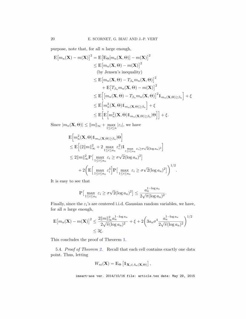
purpose, note that, for all n large enough,
E[mn(X)−m(X)
]2= E
[EΘ[mn(X,Θ)]−m(X)
]2≤ E
[mn(X,Θ)−m(X)
]2(by Jensen’s inequality)
≤ E[mn(X,Θ)− Tβnmn(X,Θ)
]2+ E
[Tβnmn(X,Θ)−m(X)
]2≤ E
[[mn(X,Θ)− Tβnmn(X,Θ)
]21mn(X,Θ)≥βn
]+ ξ
≤ E[m2n(X,Θ)1mn(X,Θ)≥βn
]+ ξ
≤ E[E[m2n(X,Θ)1mn(X,Θ)≥βn |Θ
]]+ ξ.
Since |mn(X,Θ)| ≤ ‖m‖∞ + max1≤i≤n
|εi|, we have
E[m2n(X,Θ)1mn(X,Θ)≥βn |Θ
]≤ E
[(2‖m‖2∞ + 2 max
1≤i≤anε2i )1 max
1≤i≤anεi≥σ
√2(log an)2
]≤ 2‖m‖2∞P
[max
1≤i≤anεi ≥ σ
√2(log an)2
]+ 2
(E[
max1≤i≤an
ε4i
]P[
max1≤i≤an
εi ≥ σ√
2(log an)2])1/2
.
It is easy to see that
P[
max1≤i≤an
εi ≥ σ√
2(log an)2]≤ a1−log an
n
2√π(log an)2
.
Finally, since the εi’s are centered i.i.d. Gaussian random variables, we have,for all n large enough,
E[mn(X)−m(X)
]2 ≤ 2‖m‖2∞a1−log ann
2√π(log an)2
+ ξ + 2
(3anσ
4 a1−log ann
2√π(log an)2
)1/2
≤ 3ξ.
This concludes the proof of Theorem 1.
5.4. Proof of Theorem 2. Recall that each cell contains exactly one datapoint. Thus, letting
Wni(X) = EΘ
[1Xi∈An(X,Θ)
],
imsart-aos ver. 2014/10/16 file: article.tex date: May 29, 2015
CONSISTENCY OF RANDOM FORESTS 21
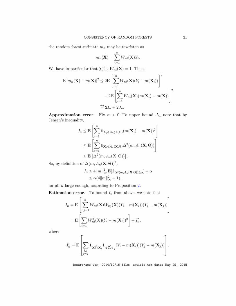
the random forest estimate mn may be rewritten as
mn(X) =
n∑i=1
Wni(X)Yi.
We have in particular that∑n
i=1Wni(X) = 1. Thus,
E [mn(X)−m(X)]2 ≤ 2E
[n∑i=1
Wni(X)(Yi −m(Xi))
]2
+ 2E
[n∑i=1
Wni(X)(m(Xi)−m(X))
]2
def= 2In + 2Jn.
Approximation error. Fix α > 0. To upper bound Jn, note that byJensen’s inequality,
Jn ≤ E
[n∑i=1
1Xi∈An(X,Θ)(m(Xi)−m(X))2
]
≤ E
[n∑i=1
1Xi∈An(X,Θ)∆2(m,An(X,Θ))
]≤ E
[∆2(m,An(X,Θ))
].
So, by definition of ∆(m,An(X,Θ))2,
Jn ≤ 4‖m‖2∞E[1∆2(m,An(X,Θ))≥α] + α
≤ α(4‖m‖2∞ + 1),
for all n large enough, according to Proposition 2.
Estimation error. To bound In from above, we note that
In = E
n∑i,j=1
Wni(X)Wnj(X)(Yi −m(Xi))(Yj −m(Xj))
= E
[∑i=1
W 2ni(X)(Yi −m(Xi))
2
]+ I ′n,
where
I ′n = E
∑i,ji 6=j
1X
Θ↔Xi1X
Θ′↔Xj
(Yi −m(Xi))(Yj −m(Xj))
.imsart-aos ver. 2014/10/16 file: article.tex date: May 29, 2015
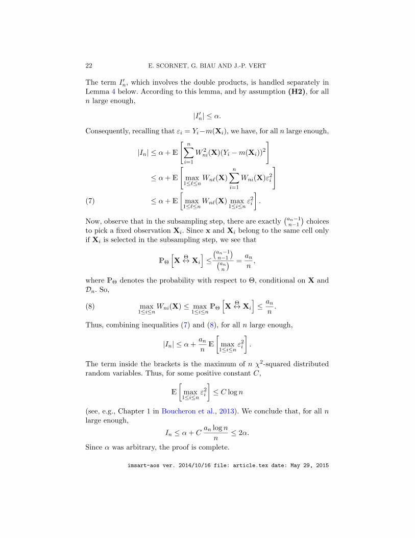
22 E. SCORNET, G. BIAU AND J.-P. VERT
The term I ′n, which involves the double products, is handled separately inLemma 4 below. According to this lemma, and by assumption (H2), for alln large enough,
|I ′n| ≤ α.
Consequently, recalling that εi = Yi−m(Xi), we have, for all n large enough,
|In| ≤ α+ E
[n∑i=1
W 2ni(X)(Yi −m(Xi))
2
]
≤ α+ E
[max
1≤`≤nWn`(X)
n∑i=1
Wni(X)ε2i
]
≤ α+ E
[max
1≤`≤nWn`(X) max
1≤i≤nε2i
].(7)
Now, observe that in the subsampling step, there are exactly(an−1n−1
)choices
to pick a fixed observation Xi. Since x and Xi belong to the same cell onlyif Xi is selected in the subsampling step, we see that
PΘ
[X
Θ↔ Xi
]≤(an−1n−1
)(ann
) =ann,
where PΘ denotes the probability with respect to Θ, conditional on X andDn. So,
max1≤i≤n
Wni(X) ≤ max1≤i≤n
PΘ
[X
Θ↔ Xi
]≤ an
n.(8)
Thus, combining inequalities (7) and (8), for all n large enough,
|In| ≤ α+annE
[max
1≤i≤nε2i
].
The term inside the brackets is the maximum of n χ2-squared distributedrandom variables. Thus, for some positive constant C,
E
[max
1≤i≤nε2i
]≤ C log n
(see, e.g., Chapter 1 in Boucheron et al., 2013). We conclude that, for all nlarge enough,
In ≤ α+ Can log n
n≤ 2α.
Since α was arbitrary, the proof is complete.
imsart-aos ver. 2014/10/16 file: article.tex date: May 29, 2015
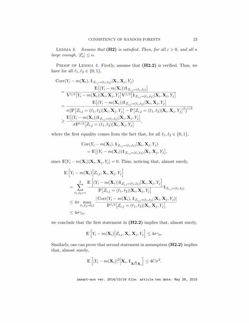
CONSISTENCY OF RANDOM FORESTS 23
Lemma 4. Assume that (H2) is satisfied. Then, for all ε > 0, and all nlarge enough, |I ′n| ≤ α.
Proof of Lemma 4. Firstly, assume that (H2.2) is verified. Thus, wehave for all `1, `2 ∈ {0, 1},
Corr(Yi −m(Xi),1Zi,j=(`1,`2)|Xi,Xj , Yj)
=E[(Yi −m(Xi))1Zi,j=(`1,`2)
]V1/2
[Yi −m(Xi)|Xi,Xj , Yj
]V1/2
[1Zi,j=(`1,`2)|Xi,Xj , Yj
]=
E[(Yi −m(Xi))1Zi,j=(`1,`2)|Xi,Xj , Yj
]σ(P[Zi,j = (`1, `2)|Xi,Xj , Yj
]− P
[Zi,j = (`1, `2)|Xi,Xj , Yj
]2)1/2≥E[(Yi −m(Xi))1Zi,j=(`1,`2)|Xi,Xj , Yj
]σP1/2
[Zi,j = (`1, `2)|Xi,Xj , Yj
] ,
where the first equality comes from the fact that, for all `1, `2 ∈ {0, 1},
Cov(Yi −m(Xi),1Zi,j=(`1,`2)|Xi,Xj , Yj)
= E[(Yi −m(Xi))1Zi,j=(`1,`2)|Xi,Xj , Yj
],
since E[Yi −m(Xi)|Xi,Xj , Yj ] = 0. Thus, noticing that, almost surely,
E[Yi −m(Xi)
∣∣∣Zi,j ,Xi,Xj , Yj
]=
2∑`1,`2=1
E[(Yi −m(Xi))1Zi,j=(`1,`2)|Xi,Xj , Yj
]P[Zi,j = (`1, `2)|Xi,Xj , Yj
] 1Zi,j=(`1,`2)
≤ 4σ max`1,`2=0,1
|Corr(Yi −m(Xi),1Zi,j=(`1,`2)|Xi,Xj , Yj)|P1/2
[Zi,j = (`1, `2)|Xi,Xj , Yj
]≤ 4σγn,
we conclude that the first statement in (H2.2) implies that, almost surely,
E[Yi −m(Xi)
∣∣∣Zi,j ,Xi,Xj , Yj
]≤ 4σγn.
Similarly, one can prove that second statement in assumption (H2.2) impliesthat, almost surely,
E[|Yi −m(Xi)|2
∣∣∣Xi,1X
Θ↔Xi
]≤ 4Cσ2.
imsart-aos ver. 2014/10/16 file: article.tex date: May 29, 2015
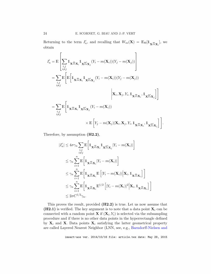
24 E. SCORNET, G. BIAU AND J.-P. VERT
Returning to the term I ′n, and recalling that Wni(X) = EΘ[1X
Θ↔Xi], we
obtain
I ′n = E
∑i,ji 6=j
1X
Θ↔Xi1X
Θ′↔Xj
(Yi −m(Xi))(Yj −m(Xj))
=∑i,ji 6=j
E
[E
[1X
Θ↔Xi1X
Θ′↔Xj
(Yi −m(Xi))(Yj −m(Xj))
∣∣∣∣∣Xi,Xj , Yi,1X
Θ↔Xi,1
XΘ′↔Xj
]]
=∑i,ji 6=j
E
[1X
Θ↔Xi1X
Θ′↔Xj
(Yi −m(Xi))
× E[Yj −m(Xj)|Xi,Xj , Yi,1
XΘ↔Xi
,1X
Θ′↔Xj
]].
Therefore, by assumption (H2.2),
|I ′n| ≤ 4σγn∑i,ji 6=j
E
[1X
Θ↔Xi1X
Θ′↔Xj
|Yi −m(Xi)|]
≤ γnn∑i=1
E
[1X
Θ↔Xi|Yi −m(Xi)|
]
≤ γnn∑i=1
E
[1X
Θ↔XiE[|Yi −m(Xi)|
∣∣∣Xi,1X
Θ↔Xi
] ]
≤ γnn∑i=1
E
[1X
Θ↔XiE1/2
[|Yi −m(Xi)|2
∣∣∣Xi,1X
Θ↔Xi
] ]≤ 2σC1/2γn.
This proves the result, provided (H2.2) is true. Let us now assume that(H2.1) is verified. The key argument is to note that a data point Xi can beconnected with a random point X if (Xi, Yi) is selected via the subsamplingprocedure and if there is no other data points in the hyperrectangle definedby Xi and X. Data points Xi satisfying the latter geometrical propertyare called Layered Nearest Neighbor (LNN, see, e.g., Barndorff-Nielsen and
imsart-aos ver. 2014/10/16 file: article.tex date: May 29, 2015
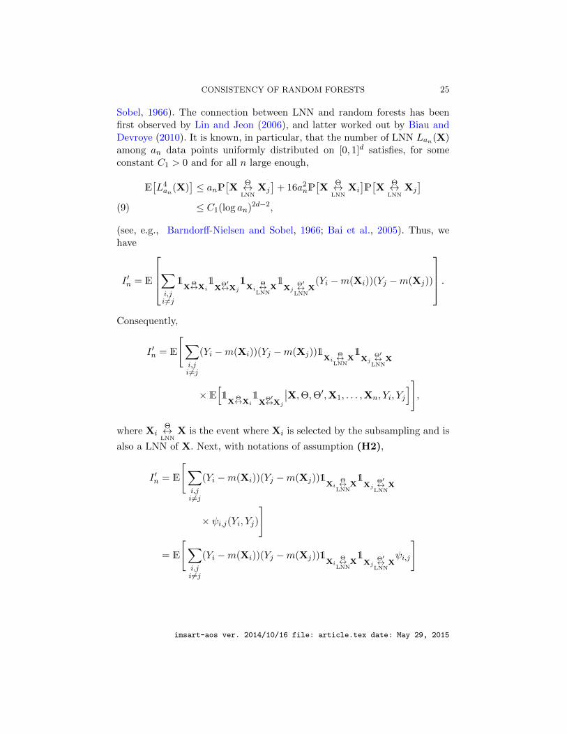
CONSISTENCY OF RANDOM FORESTS 25
Sobel, 1966). The connection between LNN and random forests has beenfirst observed by Lin and Jeon (2006), and latter worked out by Biau andDevroye (2010). It is known, in particular, that the number of LNN Lan(X)among an data points uniformly distributed on [0, 1]d satisfies, for someconstant C1 > 0 and for all n large enough,
E[L4an(X)
]≤ anP
[X
Θ↔LNN
Xj
]+ 16a2
nP[X
Θ↔LNN
Xi
]P[X
Θ↔LNN
Xj
]≤ C1(log an)2d−2,(9)
(see, e.g., Barndorff-Nielsen and Sobel, 1966; Bai et al., 2005). Thus, wehave
I ′n = E
∑i,ji 6=j
1X
Θ↔Xi1X
Θ′↔Xj
1Xi
Θ↔LNN
X1Xj
Θ′↔LNN
X(Yi −m(Xi))(Yj −m(Xj))
.Consequently,
I ′n = E
[∑i,ji 6=j
(Yi −m(Xi))(Yj −m(Xj))1Xi
Θ↔LNN
X1Xj
Θ′↔LNN
X
× E[1X
Θ↔Xi1X
Θ′↔Xj
∣∣X,Θ,Θ′,X1, . . . ,Xn, Yi, Yj
]],
where XiΘ↔
LNNX is the event where Xi is selected by the subsampling and is
also a LNN of X. Next, with notations of assumption (H2),
I ′n = E
[∑i,ji 6=j
(Yi −m(Xi))(Yj −m(Xj))1Xi
Θ↔LNN
X1Xj
Θ′↔LNN
X
× ψi,j(Yi, Yj)
]
= E
[∑i,ji 6=j
(Yi −m(Xi))(Yj −m(Xj))1Xi
Θ↔LNN
X1Xj
Θ′↔LNN
Xψi,j
]
imsart-aos ver. 2014/10/16 file: article.tex date: May 29, 2015
26 E. SCORNET, G. BIAU AND J.-P. VERT
+ E
[∑i,ji 6=j
(Yi −m(Xi))(Yj −m(Xj))1Xi
Θ↔LNN
X1Xj
Θ′↔LNN
X
× (ψi,j(Yi, Yj)− ψi,j)
].
The first term is easily seen to be zero since
E
[∑i,ji 6=j
(Yi −m(Xi))(Yj −m(Xj))1Xi
Θ↔LNN
X1Xj
Θ′↔LNN
Xψ(X,Θ,Θ′,X1, . . . ,Xn)
]
=∑i,ji 6=j
E
[1Xi
Θ↔LNN
X1Xj
Θ′↔LNN
Xψi,j
× E[(Yi −m(Xi))(Yj −m(Xj))
∣∣X,X1, . . . ,Xn,Θ,Θ′]]
= 0.
Therefore,
|I ′n| ≤ E
[∑i,ji 6=j
|Yi −m(Xi)||Yj −m(Xj)|1Xi
Θ↔LNN
X1Xj
Θ′↔LNN
X
× |ψi,j(Yi, Yj)− ψi,j |
]
≤ E
[max
1≤`≤n|Yi −m(Xi)|2 max
i,ji 6=j
|ψi,j(Yi, Yj)− ψi,j |
×∑i,ji 6=j
1Xi
Θ↔LNN
X1Xj
Θ′↔LNN
X
].
Now, observe that ∑i,ji 6=j
1Xi
Θ↔LNN
X1Xj
Θ′↔LNN
X≤ L2
an(X),
imsart-aos ver. 2014/10/16 file: article.tex date: May 29, 2015

CONSISTENCY OF RANDOM FORESTS 27
Consequently,
|I ′n| ≤ E1/2
[L4an(X) max
1≤`≤n|Yi −m(Xi)|4
]
× E1/2
[maxi,ji 6=j
|ψi,j(Yi, Yj)− ψi,j |
]2
.(10)
Simple calculations reveal that there exists C1 > 0 such that, for all n,
E[
max1≤`≤n
|Yi −m(Xi)|4]≤ C1(log n)2.(11)
Thus, by inequalities (9) and (11), the first term in (10) can be upperbounded as follows:
E1/2
[L4an(X) max
1≤`≤n|Yi −m(Xi)|4
]
= E1/2
[L4an(X)E
[max
1≤`≤n|Yi −m(Xi)|4
∣∣X,X1, . . . ,Xn
]]≤ C ′(log n)(log an)d−1.
Finally,
|I ′n| ≤ C ′(log an)d−1(log n)α/2E1/2
[maxi,ji 6=j
|ψi,j(Yi, Yj)− ψi,j |
]2
,
which tends to zero by assumption.
SUPPLEMENTARY MATERIAL
Supplement A: Technical results(doi: COMPLETED BY THE TYPESETTER; .pdf). Proofs of technicalresults
Acknowledgements. This work was supported by the European Re-search Council [SMAC-ERC-280032]. We greatly thank two referees for valu-able comments and insightful suggestions.
imsart-aos ver. 2014/10/16 file: article.tex date: May 29, 2015

28 E. SCORNET, G. BIAU AND J.-P. VERT
References.
D. Amaratunga, J. Cabrera, and Y.-S. Lee. Enriched random forests. Bioinformatics, 24:2010–2014, 2008.
Z.-H. Bai, L. Devroye, H.-K. Hwang, and T.-H. Tsai. Maxima in hypercubes. RandomStructures & Algorithms, 27:290–309, 2005.
O. Barndorff-Nielsen and M. Sobel. On the distribution of the number of admissible pointsin a vector random sample. Theory of Probability & Its Applications, 11:249–269, 1966.
G. Biau. Analysis of a random forests model. Journal of Machine Learning Research, 13:1063–1095, 2012.
G. Biau and L. Devroye. On the layered nearest neighbour estimate, the bagged near-est neighbour estimate and the random forest method in regression and classification.Journal of Multivariate Analysis, 101:2499–2518, 2010.
G. Biau, L. Devroye, and G. Lugosi. Consistency of random forests and other averagingclassifiers. Journal of Machine Learning Research, 9:2015–2033, 2008.
S. Boucheron, G. Lugosi, and P. Massart. Concentration inequalities: A nonasymptotictheory of independence. Oxford University Press, 2013.
E. Bradley. The jackknife, the bootstrap and other resampling plans, volume 38. SIAM,1982.
L. Breiman. Bagging predictors. Machine Learning, 24:123–140, 1996.L. Breiman. Random forests. Machine Learning, 45:5–32, 2001.L. Breiman. Consistency for a simple model of random forests. Technical Report 670, UC
Berkeley, 2004.L. Breiman, J. Friedman, R.A. Olshen, and C.J. Stone. Classification and Regression
Trees. Chapman & Hall, New York, 1984.P. Buhlmann and B. Yu. Analyzing bagging. The Annals of Statistics, 30:927–961, 2002.S. Clemencon, M. Depecker, and N. Vayatis. Ranking forests. Journal of Machine Learning
Research, 14:39–73, 2013.D.R. Cutler, T.C. Edwards Jr, K.H. Beard, A. Cutler, K.T. Hess, J. Gibson, and J.J.
Lawler. Random forests for classification in ecology. Ecology, 88:2783–2792, 2007.M. Denil, D. Matheson, and N. de Freitas. Consistency of online random forests. In
Proceedings of the ICML Conference, 2013. arXiv:1302.4853.L. Devroye, L. Gyorfi, and G. Lugosi. A Probabilistic Theory of Pattern Recognition.
Springer, New York, 1996.R. Dıaz-Uriarte and S. Alvarez de Andres. Gene selection and classification of microarray
data using random forest. BMC Bioinformatics, 7:1–13, 2006.R. Genuer. Variance reduction in purely random forests. Journal of Nonparametric Statis-
tics, 24:543–562, 2012.P. Geurts, D. Ernst, and L. Wehenkel. Extremely randomized trees. Machine Learning,
63:3–42, 2006.L. Gyorfi, M. Kohler, A. Krzyzak, and H. Walk. A Distribution-Free Theory of Nonpara-
metric Regression. Springer, New York, 2002.T. Hastie and R. Tibshirani. Generalized additive models. Statistical Science, 1:297–310,
1986.T. Hastie, R. Tibshirani, and J. Friedman. The Elements of Statistical Learning. Second
Edition. Springer, New York, 2009.H. Ishwaran and U.B. Kogalur. Consistency of random survival forests. Statistics &
Probability Letters, 80:1056–1064, 2010.H. Ishwaran, U.B. Kogalur, E.H. Blackstone, and M.S. Lauer. Random survival forests.
The Annals of Applied Statistics, 2:841–860, 2008.
imsart-aos ver. 2014/10/16 file: article.tex date: May 29, 2015

CONSISTENCY OF RANDOM FORESTS 29
A. Kleiner, A. Talwalkar, P. Sarkar, and M.I. Jordan. A scalable bootstrap for massivedata. Journal of the Royal Statistical Society: Series B (Statistical Methodology), 76:795–816, 2014.
Y. Lin and Y. Jeon. Random forests and adaptive nearest neighbors. Journal of theAmerican Statistical Association, 101:578–590, 2006.
N. Meinshausen. Quantile regression forests. Journal of Machine Learning Research, 7:983–999, 2006.
L. Mentch and G. Hooker. Ensemble trees and clts: Statistical inference for supervisedlearning. arXiv:1404.6473, 2014.
A. Nobel. Histogram regression estimation using data-dependent partitions. The Annalsof Statistics, 24:1084–1105, 1996.
D.N. Politis, J.P. Romano, and M. Wolf. Subsampling. Springer, New York, 1999.A.M. Prasad, L.R. Iverson, and A. Liaw. Newer classification and regression tree tech-
niques: Bagging and random forests for ecological prediction. Ecosystems, 9:181–199,2006.
E. Scornet. On the asymptotics of random forests. arXiv:1409.2090, 2014.E. Scornet, G. Biau, and J.-P. Vert. Supplementary materials for : Consistency of random
forests. 2015.J. Shotton, A. Fitzgibbon, M. Cook, T. Sharp, M. Finocchio, R. Moore, A. Kipman,
and A. Blake. Real-time human pose recognition in parts from single depth images.In Proceedings of the IEEE Conference on Computer Vision and Pattern Recognition,pages 1297–1304, 2011.
C.J. Stone. Consistent nonparametric regression. The Annals of Statistics, 5:595–645,1977.
C.J. Stone. Additive regression and other nonparametric models. The Annals of Statistics,pages 689–705, 1985.
V. Svetnik, A. Liaw, C. Tong, J.C. Culberson, R.P. Sheridan, and B.P. Feuston. Randomforest: A classification and regression tool for compound classification and QSAR mod-eling. Journal of Chemical Information and Computer Sciences, 43:1947–1958, 2003.
S. Wager. Asymptotic theory for random forests. arXiv:1405.0352, 2014.S. Wager, T. Hastie, and B. Efron. Confidence intervals for random forests: The jackknife
and the infinitesimal jackknife. The Journal of Machine Learning Research, 15:1625–1651, 2014.
R. Zhu, D. Zeng, and M.R. Kosorok. Reinforcement learning trees. Technical Report,University of North Carolina, 2012.
E-mail: [email protected] E-mail: [email protected]
E-mail: [email protected]
imsart-aos ver. 2014/10/16 file: article.tex date: May 29, 2015


![Ronan & Erwan Bouroullec Design1].pdf · Created Date: 3/29/2012 2:34:11 PM](https://img.pdfslide.us/doc/110x75/60b7629ba7bdfe147951e39e/ronan-erwan-bouroullec-1pdf-created-date-3292012-23411-pm.jpg)