Embed Size (px)
Citation preview

Essays in the Labor Economics of Healthcare
By
Erin Metcalf Johnson
A dissertation submitted in partial satisfaction of the
requirements for the degree of
Doctor of Philosophy
in
Economics
in the
Graduate Division
of the
University of California, Berkeley
Committee in charge:
Professor David Card, ChairProfessor Enrico MorettiProfessor Steven RaphaelProfessor Patrick Kline
Spring 2010

Essays in the Labor Economics of Healthcare
Copyright 2010by
Erin Metcalf Johnson

1
Abstract
Essays in the Labor Economics of Healthcare
by
Erin Metcalf Johnson
Doctor of Philosophy in Economics
University of California, Berkeley
Professor David Card, Chair
This dissertation uses tools and models from labor economics to study two infor-mation problems in healthcare markets: the uncertainty of patients regarding thequality of medical care and the asymmetry of information between physicians andpatients. These problems may lead to market failure and impact patient care,but our current understanding of the consequences of each is imperfect.
I first consider patients’ difficulty in determining the quality of medical services,focusing on technical skill of cardiac specialists. While it is difficult for patientsto judge the skill of cardiac specialists due to information problems, referring doc-tors may have access to quality information unavailable to patients. This chapterconsiders whether the referral relationship between primary care physicians andspecialists mitigates problems arising from patients’ lack of information in thiscontext. In particular, I measure the extent to which referring doctors learnabout specialist quality by observing patient outcomes and use this informationto select specialists on patients’ behalf.
This chapter presents a model of the referral relationship with public learningby PCPs about specialist quality. The model makes predictions for specialists’careers. In general terms, the model predicts that careers of specialists shoulddiverge by quality over time. I test predictions of the model using the uni-verse of Medicare claims filed by cardiac specialists in the U.S. from 1996-2005.Specifically, I compare careers of higher and lower quality specialists using a newmeasure of specialist quality that is robust to nonrandom patient sorting. Theevidence suggests some degree of learning by PCPs: lower quality specialists aresignificantly more likely to drop out of the labor market and to change geographicmarkets over time. For young cohorts, learning also results in improved sortingof patients to providers based on risk characteristics over time.

2
The next chapter, which is joint work with M. Marit Rehavi, addresses the asym-metry of information between physicians and patients. Specifically, it measuresthe extent of agency problems arising from this inequality, focusing on the deci-sion to perform C-sections. We do this by comparing the probability of receivinga C-section for physician-patients with the probability for non-physician profes-sionals. The research design exploits the fact that physicians are better informedregarding the appropriateness of recommendations and treatments than the aver-age professional. As such, treatments for this group provide a near-fully-informedbaseline that allows us to isolate the effects of information and agency problems.
We carry out this analysis using vital statistics data from the state of Texas,including every registered birth from 1995-2008. We find evidence consistentwith agency problems in the physician-patient relationship. Physician-patientsare approximately 5% less likely to have a C-section than other highly educatedpatients, controlling for relevant medical factors. This difference is even largerwhen the mother is the physician, and it comes almost entirely from non-emergecyC-sections. Findings are consistent with significant agency problems, and theseappear to have increased in importance over the sample period.

i
This dissertation is dedicated to my family, especially my husband,Keith Johnson, and my parents, Jack and Nancy Metcalf.

ii
Contents
List of Figures iii
List of Tables iv
Acknowledgments v
1 Introduction and Overview 1
2 Ability, Learning and the Career Path of Cardiac Specialists 42.1 Introduction . . . . . . . . . . . . . . . . . . . . . . . . . . . . . . 42.2 Previous Literature . . . . . . . . . . . . . . . . . . . . . . . . . . 92.3 Setup and Model . . . . . . . . . . . . . . . . . . . . . . . . . . . 11
2.3.1 Practice Setting . . . . . . . . . . . . . . . . . . . . . . . . 112.3.2 Model . . . . . . . . . . . . . . . . . . . . . . . . . . . . . 13
2.4 Empirical Approach . . . . . . . . . . . . . . . . . . . . . . . . . . 202.4.1 Data . . . . . . . . . . . . . . . . . . . . . . . . . . . . . . 202.4.2 Constructing Doctor Quality Measures . . . . . . . . . . . 22
2.5 Empirical Evidence . . . . . . . . . . . . . . . . . . . . . . . . . . 262.6 Conclusion . . . . . . . . . . . . . . . . . . . . . . . . . . . . . . . 322.7 Figures . . . . . . . . . . . . . . . . . . . . . . . . . . . . . . . . . 342.8 Tables . . . . . . . . . . . . . . . . . . . . . . . . . . . . . . . . . 37
3 Agency Issues in Medicine: Evidence from Cesarean Sections 543.1 Introduction . . . . . . . . . . . . . . . . . . . . . . . . . . . . . . 543.2 Previous Literature . . . . . . . . . . . . . . . . . . . . . . . . . . 573.3 Empirical Approach . . . . . . . . . . . . . . . . . . . . . . . . . . 593.4 Empirical Evidence . . . . . . . . . . . . . . . . . . . . . . . . . . 623.5 Conclusion . . . . . . . . . . . . . . . . . . . . . . . . . . . . . . . 653.6 Figures . . . . . . . . . . . . . . . . . . . . . . . . . . . . . . . . . 673.7 Tables . . . . . . . . . . . . . . . . . . . . . . . . . . . . . . . . . 70
A Appendix to Chapter 3 85

iii
List of Figures
2.1 CABG, PCI and Stent Claims Over Time . . . . . . . . . . . . . . . 342.2 Time Trends in Referral Volumes by Dropout Status - ICs . . . . . . 352.3 Time Trends in Referral Volumes by Dropout Status - CT Surgeons . 36
3.1 C-section Rates, U.S. and Texas, 1995-2007 . . . . . . . . . . . . . . 673.2 State C-section Rates for Doctors and Non-doctors, 1995-2007 . . . . 683.3 Gap in C-section Rates for Doctors and Non-doctors Over Time . . . 69

iv
List of Tables
2.1 Physician Summary Statistics . . . . . . . . . . . . . . . . . . . . 372.2 Patient Level Summary Statistics . . . . . . . . . . . . . . . . . . 382.3 Coefficients from Correlated Random Effects Logits - PCI Sample 392.3 (continued) . . . . . . . . . . . . . . . . . . . . . . . . . . . . . . 402.4 Coefficients from Correlated Random Effects Logits - CABG Sample 412.4 (continued) . . . . . . . . . . . . . . . . . . . . . . . . . . . . . . 422.5 Doctor Quality Measures . . . . . . . . . . . . . . . . . . . . . . . 432.6 Doctor Quality Measures Over Time . . . . . . . . . . . . . . . . 442.7 Doctor Quality Measures Controlling for Patient Sorting . . . . . 452.8 Dropout Analysis . . . . . . . . . . . . . . . . . . . . . . . . . . . 462.9 Moves Analysis . . . . . . . . . . . . . . . . . . . . . . . . . . . . 472.10 Analysis of Referral Volumes . . . . . . . . . . . . . . . . . . . . . 482.11 Analysis of Referral Volumes - Robustness . . . . . . . . . . . . . 492.12 Analysis of Referral Volumes - Quantile Regressions . . . . . . . . 502.13 Analysis of Referral Volumes - CT Surgeons in New York State . 512.14 Analysis of Patient Risk Characteristics - Young Cohorts . . . . . 522.15 Patient Risk Factors Analysis . . . . . . . . . . . . . . . . . . . . 53
3.1 Delivery Outcomes for Doctors and Non-doctors . . . . . . . . . . 703.2 Delivery Outcomes for Doctors and Non-doctors . . . . . . . . . . 713.3 Summary Statistics, 1995-April 2008 . . . . . . . . . . . . . . . . 723.4 Summary Statistics, 2005-April 2008 . . . . . . . . . . . . . . . . 733.5 C-section Rates for Doctors and Non-doctors . . . . . . . . . . . . 743.6 C-section Rates for Lawyers and Nurses . . . . . . . . . . . . . . . 753.7 Breakdown of Delivery Outcomes for Doctors and Non-doctors . . 763.8 Birth Outcomes for Doctors and Non-doctors . . . . . . . . . . . 77
A.1 C-Section Rates for Doctors and High-Educated Non-doctors, FullCoefficient List . . . . . . . . . . . . . . . . . . . . . . . . . . . . 85
A.1 (continued) . . . . . . . . . . . . . . . . . . . . . . . . . . . . . . 86

v
Acknowledgments
I am enormously indebted to David Card. In our interactions over the pastfive years, David helped me decide what sort of economist I want to be and thenhe trained me to that purpose. I am grateful for his gifts of time and thought andfor his guidance and example. In addition to this, I am grateful for his patienceand good humor in supporting my progress and for his many, many contributionsto this work.
I am also grateful to the members of my dissertation committee for theiradvice throughout my graduate school experience. I am especially appreciativeof Enrico Moretti for thoughtful suggestions on several projects, and of PatrickKline for insights that significantly improved this work. I also received helpfulcomments from my fellow graduate students and seminar participants in thedepartment. I owe particular thanks to Ashley Langer, Erin Syron, and MaritRehavi.
Several professors provided valuable guidance early in my training. I amgrateful to my undergraduate thesis advisor, Jonathan Parker, for introducing meto research and setting me on this career path; I am thankful to Jeff Liebman forbeginning my training and providing invaluable career advice; and I am gratefulto Alan Auerbach and Ronald Lee for teaching me research skills and advisingmy choice of topics in my first years at Berkeley.
Finally, I thank my family for making this education possible. Thanks alsoto my father for serving as a sounding board and source of medical knowledgeand to Keith for solving all my technical problems.

1
Chapter 1
Introduction and Overview
It has long been recognized that health care markets differ from the canonicalefficient market. Kenneth Arrow delineates characteristics of medical care whichdifferentiate it from the usual commodity in his 1963 paper titled “Uncertaintyand the Welfare Economics of Medical Care.” He writes that “the risk and uncer-tainty in medical care” combined with “the nonexistence of markets for bearingsome of these risks” results in several departures from the competitive model.
One such departure arises from the difficulty for consumers in judging thequality of medical care. Arrow writes, “Uncertainty as to the quality of theproduct is perhaps more intense here than in any other important commodity.”He continues, “In most commodities, the possibility of learning from one’s ownexperience or that of others is strong because there is an adequate number oftrials. In the case of severe illness, that is, in general, not true; the uncertaintydue to inexperience is added to the intrinsic difficulty of prediction.”
Another departure of health care markets from the competitive standardarises from the fact that physicians have more information than patients regardingpatients’ treatment options and need for medical care. Arrow writes of thisasymmetry of information,
“Under ideal insurance the patient would actually have no concernwith the informational inequality between himself and the physician,since he would only be paying by results anyway, and his utility po-sition would in fact be thoroughly guaranteed. In its absence hewants to have some guarantee that at least the physician is using hisknowledge to the best advantage. This leads to the setting up of arelationship of trust and confidence, one which the physician has asocial obligation to live up to. Since the patient does not, at leastin his belief, know as much as the physician, he cannot completelyenforce standards of care.”

2
These two information problems are the focus of this dissertation. In thefollowing chapters, I use tools and models from labor economics to measure theimpacts of each of these market failures on delivery of care and patient outcomes.I first consider patients’ uncertainty regarding the quality of medical care. Inthis chapter, I determine the extent to which referring doctors know about andlearn about specialist quality, focusing on cardiac specialists. While it is difficultfor patients to judge the skill of cardiac specialists due to information problems,referring doctors may have access to quality information unavailable to patients.This chapter uncovers how referring doctors use available information. In partic-ular, the paper asks how market learning by referring doctors affects specialistcareers. In so doing, it informs as to the nature of problems arising from patients’lack of information and the quality incentives faced by specialists.
First I present a model of the referral relationship based on models of em-ployer learning from labor economics. In the model referring doctors observepatient outcomes and use this information to determine specialist quality andallocate patients to specialists. The model makes three predictions for special-ists’ careers: first, under learning by referring doctors, lower quality specialistswill be more likely to drop out of practice over time; second, specialists will sortacross markets based on quality; and third, referring doctors will seek to allocatehigher risk patients to higher quality doctors as quality becomes known. I testthese predictions using the universe of Medicare claims filed by cardiac special-ists in the U.S. from 1996-2005. Specifically, I compare careers of higher andlower quality specialists using a new measure of specialist quality that is robustto nonrandom patient sorting. The evidence suggests some degree of learningby referring doctors, though the labor market is far from the competitive bench-mark. I find that lower quality specialists are significantly more likely to dropout of the labor market and to change geographic markets over time. For youngcohorts, learning also results in improved sorting of patients to providers basedon risk characteristics over time.
The next chapter, which is joint work with M. Marit Rehavi, addresses theasymmetry of information between physicians and patients. This chapter mea-sures the extent of agency problems arising from this inequality, focusing on thedecision to perform C-sections.
Physicians are thought to face incentives to perform C-sections in lieu ofvaginal deliveries.1 Response of physicians to these incentives in conflict with pa-tient interests or preferences is an example of an agency problem. To determinewhether doctors exploit the asymmetry of information between themselves andtheir patients to perform costly unnecessary C-sections, we compare the prob-
1These incentives may be financial, as C-sections are typically reimbursed at a higher rate,or they may arise from malpractice concerns or convenience factors.

3
ability of receiving a C-section for physician-patients with the probability fornon-physician professionals. Because physicians have medical knowledge, theyshould be able to determine the appropriateness of their doctors’ recommenda-tions and of the treatment they receive. As such, there should be much lesscapacity for doctors to act in conflict with patient interest for this population,and the comparison of treatments for doctors and non-doctors is informative asto the extent of agency problems.
We carry out this analysis using vital statistics data from the state of Texas,including every registered birth from 1995-2008. We find evidence consistentwith agency problems in the physician-patient relationship. Physician-patientsare approximately 5% less likely to have a C-section than other highly educatedpatients, controlling for relevant medical factors. This difference is even largerwhen the mother is the physician, and it comes almost entirely from non-emergecyC-sections. Findings suggest significant agency problems in this context, andthese have increased over the sample period. However, the increase in agencyproblems can explain only a small fraction of the increase in C-sections over theperiod.

4
Chapter 2
Ability, Learning and the CareerPath of Cardiac Specialists
There is a large literature in economics on the role of learning by employersin labor markets. This chapter applies insights from this literature to the referralrelationship between primary care physicians (PCPs) and cardiac specialists inmedicine to study the nature and strength of the quality incentives specialistsface. I present a model of the referral relationship with public learning by PCPsabout specialist quality. The model makes three predictions for specialists’ ca-reers: first, under learning by PCPs lower quality specialists will be more likely todrop out of practice over time; second, specialists will sort across markets basedon quality; and third, PCPs will seek to allocate higher risk patients to higherquality doctors as quality becomes known. I test these predictions using the uni-verse of Medicare claims filed by cardiac specialists in the U.S. from 1996-2005.Specifically, I compare careers of higher and lower quality specialists using a newmeasure of specialist quality that is robust to nonrandom patient sorting. Theevidence suggests some degree of learning by PCPs: lower quality specialists aresignificantly more likely to drop out of the labor market and to change geographicmarkets over time. For young cohorts, learning also results in improved sortingof patients to providers based on risk characteristics over time. However, condi-tional on remaining in a local market, specialists’ procedure volumes and chargesdo not respond to quality.
2.1 IntroductionThere is a growing interest among policymakers in measuring the quality of
care provided by physicians and in enhancing incentives for quality care. Thisinterest has arisen in part from recent studies that show notable differences in

Section 2.1. Introduction 5
patient mortality rates across providers.1 It has also been driven by an increasingawareness of the role that physicians play in allocating health resources. Inthe U.S. health system physicians oversee the majority of decisions regardinghealthcare usage. Specialists in particular are often gatekeepers for the typesof new technologies thought to be driving growth in health spending (Newhouse(1992)).
This growing interest in health care quality has led to a large empirical liter-ature on the effects of quality programs. Examples include the physician “reportcard” literature, which measures reactions to the publication of individual physi-cians’ patient outcomes (typically mortality rates in complex procedures).2 Otherrecent studies address incentives arising from pay-for-performance programs3 andfrom contracting schemes implemented in HMOs and group practices.4 However,there is relatively little work on one of the most important potential incentivemechanisms in professional service relationships: the role of “market learning”about the relative quality (or “ability”) of individual professionals.
There is reason to believe that such incentives are important in physicianlabor markets. Most specialists receive the majority of their patients as refer-rals from primary care physicians (PCPs), and PCPs observe patient outcomesfollowing specialist care. In this paper I draw from the large literature on em-ployer learning in economics to illuminate the incentives arising in the referralrelationship between PCPs and specialists. I present a simple model of the refer-ral relationship that makes testable predictions about the careers of specialists inthe presence of learning by PCPs. I then test these predictions using Medicareclaims data for the universe of cardiac specialists in the U.S. from 1996-2005.
The model builds on the public learning model of Jovanovic (1979) andFarber and Gibbons (1996).5 I assume that PCPs update their expectations of
1For example, Hannan et al. (1990), O’Connor et al. (1991), Williams, Nash and Goldfarb(1991), and McClellan and Staiger (1999).
2See Hannan et al. (1994), Green and Wintfeld (1995), Schneider and Epstein (1996),Peterson et al. (1998), Cutler et al. (2004), and Dranove et al. (2003). See also two recentpapers that have employed models from labor economics and industrial organization in thehealth arena to illuminate incentives arising from cardiac surgeon report cards (Glazer, McGuireand Newhouse (2007), Fong (2009)).
3For example, Rosenthal et al. (2005), Campbell et al (2007) and Mullen, Frank and Rosen-thal (2009), and Rosenthal and Frank (2006) provides a review.
4For example, Hemenway (1990), Gaynor and Pauly (1990), LeGrand (1999), Gaynor, Reb-itzer and Taylor (2001), and Barro and Beaulieu (2003).
5I primarily draw from the models of Jovanovic (1979), Farber and Gibbons (1996) andAltonji and Pierret (1999). These authors develop public learning models to investigate learningby employers about employee ability. I also draw insights from Fama (1980), Lazear and Rosen(1981), Harris and Holmstrom (1982), Gibbons and Murphy (1992), and Chevalier and Ellison(1997), who consider the importance of career concerns in labor markets; and Greenwald (1986)and Gibbons and Katz (1991), who explore the case of asymmetric employer learning.

Section 2.1. Introduction 6
specialists’ ability over time given observed patient outcomes and that they al-locate referrals to specialists to improve patient survival. I augment the basiclearning framework to allow for capacity constraints, which are an important in-stitutional feature of cardiac specialty markets, and I allow patients to differ inrisk characteristics. The model has three main predictions. First, when PCPsare learning about the quality of specialists, lower quality specialists will be morelikely to drop out of practice over time. Second, specialists will sort across mar-kets based on quality - lower quality specialists can potentially avoid reductionsin referrals by moving to markets with capacity constraints. Third, PCPs willseek to allocate higher risk patients to higher quality doctors as quality becomesknown.
The empirical analysis focuses on two types of cardiac specialists: inter-ventional cardiologists (ICs), who perform angioplasty, and cardiothoracic (CT)surgeons, who perform coronary artery bypass graft surgery (CABG). For bothof these specialties over 45% of patients are over 65 and observable in Medicareclaims data.6 Further, both practices are procedure-based and technical skill isan important determinant of patient outcomes in PCI and CABG. These spe-cialties have also been at the center of the quality reporting movement: whileCT surgery was the original focus, several states and agencies have recently alsobegun reporting quality information for ICs. The use of data on the two types ofspecialists also allows me to exploit the proliferation of the bare metal stent dur-ing the sample period, which increased demand for PCI and decreased demandfor CABG (Cutler and Huckman (2003)), to determine how incentives differ ingrowing and declining markets.
The labor market for medical specialists is unique, and ex ante the empiricalmagnitude of any learning effect is unclear. On the one hand, referring doctorshave access to much of the quality information published in physician report cards– they observe their own patients’ outcomes following specialist care, and theycan also gather information from colleagues and hospital review committees. Onthe other hand, the long and arduous nature of specialty training may suggesta more limited role for learning than in labor markets for high school or collegegraduates. Further, the low rate of patient mortality and the small numbers ofpatient procedures performed by some doctors may make it difficult for PCPs toeffectively determine specialist quality. Moreover, PCPs motivation to improvepatient survival might not be as strong as the profit maximization motivation infirms.
To empirically determine the importance of learning in physician labor mar-kets, one first needs a measure of doctor quality. Unlike in the employer learning
6This is based on analysis of hospital discharge data from the state of Florida. Adjustmentwas made for the aged population in this state.

Section 2.1. Introduction 7
case where employee productivity is generally unobserved, I observe patient mor-tality outcomes following procedures with specific doctors. I draw on severalrecent literatures to develop a new methodology for measuring specialist qual-ity. Specifically, I augment the quality measurement methods developed in thebiostatistics literature on hospital quality (Localio et al. (1997), Burgess et al.(2000), Thomas et al. (1994), and Normand et al. (1997)) to allow for fornon-random sorting of patients to individual specialists, using the correlated ran-dom effects method of Mundlak (1978) and Chamberlain (1982). Like the recent“teacher quality” literature, I implement an empirical Bayes procedure (Morris(1983), McClellan and Staiger (1999)) to obtain quality measures that accountfor estimation error in the random effects procedure.7
This first step in the analysis is interesting in its own right: in constructingthese measures, I demonstrate that there is substantial, measurable variation inquality across specialists after accounting for estimation error. I also show thatquality measured in this way is informative over the career - that is, measuresconstructed during the first four years of the sample predict patient mortality forthe next six years of a specialist’s career. Finally, I find that failing to controlfor non-random sorting of patients substantially penalizes doctors treating highrisk patients.
Using these quality measures, I first test the prediction that lower qualityspecialists should be more likely to stop performing PCI or CABG or to dropout of practice. Intuitively, as quality becomes known over time, referrals ofhigher and lower quality specialists will diverge, with lower quality specialistsreceiving relatively fewer referrals. This in turn makes the outside option moreattractive for lower versus higher quality specialists. I consider two differentoutside options: one in which specialists stop performing procedures and adopta more clinical practice, and one in which specialists stop practicing altogether.Logistic regressions of dropout indicators on quality measures reveal that lowerquality ICs are in fact more likely to stop doing PCI. The effect is significant bothstatistically and economically: a one standard deviation decrease in doctor qualityincreases the likelihood of dropping out of performing PCI by one percentagepoint (a 10% effect). As predicted by the model, the effect is stronger in thedeclining market for CTs: a one standard deviation decrease in quality increasesthe likelihood of dropping out of CABG by two percentage points, and low qualityCT surgeons are also more likely to drop out of practicing altogether.
Next I turn to the prediction on specialist sorting: because the impacts oflearning on referral volumes are muted in capacity constrained markets, lowerquality specialists may be able to increase their referral volumes through moving
7See, for example, Hanushek (1971), Kane and Staiger (2002), Aaronson, Barrow and Sander(2003), Rockoff (2003), Kane, Rockoff and Staiger (2006), and Jacob and Lefgren (2008).

Section 2.1. Introduction 8
to markets with a relatively lower supply of specialists. I find significant effectsin regressions of indicators for changing zip codes on quality measures. For ICs aone standard deviation decrease in quality increases the likelihood of moving bytwo percentage points; for CT surgeons the effect is again slightly stronger, threepercentage points. Results are similar if I consider moves across hospital referralregions (HRRs) and moves to HRRs that are more capacity constrained.8
Having shown the importance of moving and dropout behavior in specialistcareers, it is interesting to consider how these behaviors affect incentives forspecialists who remain in practice. In the model, dropouts and moves bothreduce local capacity and mute effects of learning on referral volumes amongproviders who remain locally in practice. Intuitively, when PCPs cannot refer totheir top choice specialist, they must move down the list until they place all oftheir patients. Thus, given the size of effects on dropout and moving behavior,we might not expect to see large effects of quality on referrals over the career. Infact, I can exclude effects on total procedures and total PCI / CABG larger than1% in absolute value for a one standard deviation change in quality. Results holdwhen I consider only HRRs with relatively high physician capacity and when Iexclude large multi-specialty physician groups.
Finally, I turn to the prediction that PCPs will increase sorting of patientsto specialists based on risk factors over the career. If high ability specialists havea relative advantage at treating high risk patients - as I demonstrate - then themodel predicts that PCPs will seek to improve patient survival through this typeof sorting. Results for the full sample of ICs and CT surgeons rule out divergencein patient risk for higher and lower quality specialists. However, when I consideryoung cohorts of specialists, for whom we expect learning to be stronger, higherquality specialists receive significantly more risky patients over time.
The empirical evidence, taken together, suggests careers of higher and lowerquality specialists differ. This divergence is consistent with some degree of learn-ing by PCPs. And results suggest potential impacts on patient welfare. Lowquality specialists stopping doing PCI or stopping practicing altogether is welfare-improving assuming adequate physician supply. Further, the sorting of higherrisk cases to better physicians, who have a comparative advantage at treatingthese cases, increases patient survival. Finally, the fact that lower quality spe-cialists are more likely to move to capacity constrained areas has distributionalconsequences, as patients in these areas may receive lower quality care.
The chapter proceeds in six sections. Section 2.2 reviews the empirical liter-ature on physician incentives, including the literature on physician report cards.Section 2.3 provides details on the practice setting and presents the model. Sec-
8A hospital referral region is defined around hospitals performing both cardiovascular surgeryand neurosurgery. It is the area in which the majority of patients are referred to the hospital.See Wennberg et al. (2008) for more detail.

Section 2.2. Previous Literature 9
tion 2.4 describes the data and the construction of doctor quality signals. Section2.5 presents the empirical evidence, and Section 2.6 concludes.
2.2 Previous LiteratureThis chapter brings together the employer learning literature from labor
economics and the literature on physician incentives in health economics. To drawinsights for physicians’ careers, I build upon the public learning model developedby Farber and Gibbons (1996).9 I also draw from the literatures consideringasymmetric learning by employers (Greenwald (1986) and Gibbons and Katz(1991)) and career concerns (Fama (1980), Lazear and Rosen (1981), Harris andHolmstrom (1982), and Gibbons and Murphy (1992)).
I utilize the employer learning framework to contribute to the literature onphysician incentives. In particular, I consider quality incentives arising frommarket learning in the informal referral relationship. In contrast to this chapter,the majority of research on physician incentives has focused on financial incentivesarising in explicit employment relationships or resulting from quality initiatives.In the former group Le Grand (1999) and Gaynor, Rebitzer and Taylor (2001)study physicians employed by Health Maintenance Organizations (the former inthe UK, the latter in the US) and find evidence that physicians adjust behavior inresponse to incentive pay. Hemenway et al. (1990) and Barro and Beaulieu (2003)consider physicians employed by hospitals and find increases in productivity inresponse to changes from salary to profit-sharing pay. Gaynor and Pauly (1990)finds similar incentive responses in a study of physicians in a group practicesetting.
In the latter group is the small empirical literature on pay-for-performanceinitiatives. Campbell et al. (2007) finds evidence that a government initiativeimplemented in the U.K. significantly improved treatment of asthma and dia-betes. However, studies considering smaller financial incentives have found littleevidence of quality improvements (Rosenthal and Frank (2006), Mullen, Frankand Rosenthal (2009)).
Also in this group is the literature on physician report cards, which eval-uates the impact of publishing physician quality scores on physician behaviorand patient mortality. This literature is of particular relevance to the currentstudy, because many of the incentives arising from publishing report cards mayalso arise absent reporting from the referral relationship. For example, if PCPs
9In this paper Farber and Gibbons draw from Jovanovic (1979) to create a model of publiclearning with testable predictions for careers. In the model employers learn about employeeability over time and reward productivity by paying employees a wage equal to expected pro-ductivity.

Section 2.2. Previous Literature 10
observe some or all of the patient outcome information used to construct reportcards, then they may seek to send patients to physicians with better patientoutcomes.
The majority of the report card literature has evaluated the CABG reportingprogram in New York State, with early studies seeking to determine impacts onpatient mortality. The most widely cited of these early studies, Hannan et al.(1994), finds a large mortality reduction and an increase in the risk factors ofpatients undergoing CABG following the publishing of report cards. Researchthat has followed has attempted to determine the causality of and the mechanismsunderlying this effect. For example, it has been hypothesized that the reduction inmortality could arise from improved provider quality if lower quality doctors stopperforming CABG or if doctors exert increased effort to improve skill. Improvedsorting of patients to providers could also improve mortality if better doctors havea relative advantage at treating high risk patients. Alternatively, the mortalityreduction could result from risk selection by doctors - if doctors choose to operateon relatively healthier patients as a means of improving their scores, then overallpatient mortality might rise absent a quality improvement.
The empirical evidence is mixed.10 Peterson et al. (1998) compare the ex-perience in New York with other states that did not implement a report cardprogram. They find larger mortality declines in New York than in control statesand no evidence that New York doctors are selecting relatively healthier patientsfor surgery. Cutler et al. (2004) also finds evidence in support of quality im-provements. Using variation across providers within New York, they find thathospitals with poor performance ratings lost healthy patients and experiencedperformance improvement relative to other hospitals. However, Dranove et. al.(2003) finds increased adverse outcomes for patients when they consider a broaderpatient population in New York. They also find evidence of risk selection, withhealthier patients being relatively more likely to receive CABG after the program.And Green and Wintfeld (1995) finds evidence that coding of patient risk factorsincreased sharply after implementation of the program.
There have also been several surveys of cardiac surgeons and referring doctorsseeking to understand the mechanism behind the mortality effect. Schneiderand Epstein (1996) presents results from a survey of doctors in Pennsylvania.They find that the large majority (87%) of referring doctors say report cardshad minimal or no influence on their referral recommendations. However, it isnot clear from the survey whether this reported lack of influence arises becausereferring doctors feel their own information is superior to report card informationor whether they do not incorporate physician quality information into referraldecisions at all.
10Epstein (2006) provides a summary of the empirical literature on physician report cards.

Section 2.3. Setup and Model 11
2.3 Setup and Model
2.3.1 Practice SettingThe empirical work in this chapter focuses on two physician specialties: in-
terventional cardiology and cardiac surgery. Interventional cardiologists are car-diologists who sub-specialize in performing interventions to open arteries in theheart that have been narrowed by coronary artery disease.11 Cardiac surgeonsare surgical specialists who treat conditions of the heart and cardiovascular sys-tem. These two specialties are completely segmented: while CT surgeons repairblockages in the heart by opening the chest in surgery and do not perform per-cutaneous interventions, ICs open arteries using only non-surgical, percutaneoustechniques.12
In this chapter I evaluate ICs and CT surgeons’ skill at performing the pri-mary procedures of each of their specialties. Percutaneous coronary interventions(PCI) are the primary procedures done by ICs. The two most common of theseprocedures are angioplasty and angioplasty with stent placement. In angioplastya balloon-tipped catheter is threaded into the heart, and the balloon is inflatedto clear arterial blockages. Since the introduction of stents in the U.S. in 1994interventions increasingly involve balloon inflation followed by the placement ofa metal scaffold-like structure, called a stent.
Coronary artery bypass graft surgery (CABG), also known as open heartsurgery, is the primary procedure done by cardiac surgeons. In CABG, the pa-tient’s chest is opened, the heart is stopped, and blood is routed to a heart-lungmachine for oxygenation. Arteries or veins are harvested from elsewhere in thepatient’s body and grafted to the heart to bypass and restore blood flow arounddiseased vessels.13
11There are three major sub-specialties of cardiology. Non-invasive cardiologists diagnoseand provide medical management of patient conditions. For example, non-invasive cardiolo-gists perform stress tests, EKGs, echocardiograms and see patients in a clinical setting. Invasivecardiologists do everything non-invasive cardiologists do plus diagnostic angiography. In diag-nostic angiography, also known as heart catheterization, a catheter is threaded into the heartand used to inject contrast agent allowing for X-ray photography of the heart vessels and as-sessment of heart function. Interventional cardiologists do everything invasive cardiologists doplus perform interventions, such as angioplasty, to open arteries in the heart that have beennarrowed by plaque.
12The training of ICs and CT surgeons diverge after medical school. ICs do a 3 year internalmedicine residency followed by a 2-3 year cardiology fellowship and 1-2 additional years oftraining in PCI as fellows in interventional cardiology. CT surgeons complete a 5 year residencyprogram in general surgery and then a 2-3 year fellowship in cardiac surgery.
13CABG is generally indicated instead of PCI for patients with more severe coronary arterydisease. However, indications for PCI have been expanding to more risky patient groups withmore severe disease over time (Bohmer, Christensen and Kenagy (2000)).

Section 2.3. Setup and Model 12
These two specialties are a good choice for studying referral relationships.For both, over 45% of patients are over 65 and observable in Medicare claimsdata.14 Further, both practices are procedure-based, and technical skill is animportant determinant of patient outcomes in both PCI and CABG. In PCI, forexample, it takes a high level of technical skill to thread the catheter into theheart and developed judgment to determine the amount of pressure used to inflatethe balloon - too much pressure can rupture the vessel, but not enough pressurecan result in re-narrowing of the artery. A less skilled technician might also havemore patient complications because the procedure takes longer or requires theinjection of larger amounts of contrast agent. In CABG, a less skilled technicianmight have increased risk of bleeding or require the patient to be on the heart-lung machine for longer. These specialties have also been at the center of thequality measurement or “report card” movement. While CT surgery was theoriginal focus, several states and agencies have recently also begun reportingquality information for ICs. The use of data on the two specialties also allows meto exploit the proliferation of the bare metal stent during the sample period. Thisinnovation increased demand for PCI and decreased demand for CABG (Cutlerand Huckman (2003)), allowing me to study how incentives differ in growing anddeclining markets.
In the U.S. the majority (58%) of cardiac specialists are in private practice.15
Physicians in private practice generally earn the majority of their income by seeingpatients and submitting claims to insurance companies for their work. Insurancecompanies then pay an administratively set price for the doctor’s work (frequentlysome predetermined fixed amount or fraction of the “allowed” amount is also paidby the patient). Thus, to cover office overhead and earn a profit, most cardiacspecialists require a steady flow of patients into their practice.
The large majority of patients in an IC practice are referred from a PCPafter the PCP has determined the patient needs cardiac care (70% for Medicarepatients). While some patients may decide to see a cardiologist on their own andothers may ignore the referral of their PCP and select a specialist based on theirown research or a friend’s advice, a substantial fraction of an ICs practice volumeis directly referred from PCPs.16 Referral patterns for CT surgeons are similar,but CT surgeons receive referrals both from PCPs and from cardiologists whohave determined patients need surgery. The intent of the models which follow is tocapture the relationship between referring doctors and specialists that generatesthis downstream flow of patients, recognizing that some patients may also come
14This is based on analysis of hospital discharge data from the state of Florida. Adjustmentwas made for the aged population in this state.
15American College of Cardiology Workforce Study, 2002.16The 2007 Center for Studying Health System Change study finds most patients rely exclu-
sively on referrals in specialist choice.

Section 2.3. Setup and Model 13
for reasons not described in the model.
2.3.2 ModelIn this section I present a simple model to illustrate the effects of learning by
PCPs on specialist careers. The model builds upon the public learning models ofFarber and Gibbons (1996) and Altonji and Pierret (1999). To begin I considerthe case in which patients are homogeneous and there are no constraints onspecialist capacity. This provides the simplest treatment and illuminates thebasic implications of learning for specialist careers. In the next section I considerextensions to the model.
PCP Learning Model
To begin let i = 1, ..., N denote PCPs and j = 1, ...,M denote specialists.Assume specialists have different ability levels and specialist ability affects patientsurvival rates, with higher skill specialists having higher patient survival rates.Further assume that individual specialist skill, ηj, is not observed by PCPs; PCPsonly have prior knowledge of the distribution of specialist skill:
ηj ∼ N(X′
jβ,1H
)(2.1)
where Xj is a vector of doctor characteristics observable to PCPs at the beginningof their careers, for example the prestige of medical school attended. Note thatskill in this setting is technical skill - for example skills associated with successfullymaneuvering the catheter into a heart vessel and repairing a blockage. I cannotobserve other dimensions of specialist skill that are also likely important forpatient satisfaction or survival, such as bedside manner or clinical diagnosticcapabilities, and so I abstract away from these here.
I also assume that PCPs observe a signal of ability, yijt, in each period.Think of this as the observed survival rate for specialist j taking into accountpatient risk characteristics. It is made up of two components: true specialist skilland a mean zero normally distributed error term, εijt.
yijt = ηj + εijt, εijt ∼ N(
0, 1h
), iid (2.2)
The error term is assumed to vary across PCPs to allow different PCPs to havedifferent information sets.
At each time t, PCPs form expectations of specialist ability based on theinformation available to them. At the beginning of a specialist’s career, thisexpectation is simply the mean of the skill distribution, X ′
jβ. But in the second

Section 2.3. Setup and Model 14
period PCP i also observes the specialist’s first period patient survival rate, yij1,and incorporates this into his expectation:
Ei2[ηj|X′
jβ, yij1] = H
H + hX′
jβ + h
H + hyij1 = w2X
′
jβ + (1− w2)yij1 (2.3)
where w2 = HH+h . The expectation is a weighted average of the prior and the
signal, with the weight on the signal increasing in its precision.Iterating on the learning model gives PCP i’s expectation in time t given
the prior and the specialist’s survival rates up until time t, yij1, ..., yij(t−1):
Eit[ηj|X′
jβ, yij1, ..., yij(t−1)] = H
H + (t− 1)hX′
jβ + h
H + (t− 1)h
s=(t−1)∑s=1
yijs
= wtX′
jβ + (1− wt)ηj + h
H + (t− 1)h
s=(t−1)∑s=1
εijs
(2.4)
where wt = HH+(t−1)h . From this equation it is evident that, as t approaches
infinity, the prior belief becomes less important and true quality becomes moreimportant in the expectation. To see this note that the weight, wt, is decreasingin t.
I model the PCP’s decision as follows: in each period PCP i decides to referhis patients to specialist j if j’s expected patient survival is above some thresh-old, q. The PCP then randomizes his patients among those specialists he hasdecided to refer to. In this decision rule, PCPs care that doctor quality is abovea threshold, perhaps the survival rate of the outside option (for example, medicalmanagement) or the local standard of care; they do not care about doctor qual-ity above q. While I cannot observe the decision rule generating referral flows,anecdotal evidence suggests this rule is consistent with PCP behavior. PCPs gen-erally maintain relationships with several specialists and allocate patients fairlyevenly among those specialists. In fact, many PCPs maintain a list of specialistslong enough to ensure all patients are seen and then direct their office staff tomanage the referral process from the list. I have also considered an alternativerule in which PCPs maximize expected patient survival by referring exclusivelyto the specialist whose expected ability is highest in his estimation. This rulemakes similar predictions for the career dynamics I consider.
Under my rule, PCP i refers to j in period t if:
Eit[ηj|X′
jβ, yij, ...yij(t−1)] > q (2.5)
From this expression I derive the probability that specialist j is above the thresh-

Section 2.3. Setup and Model 15
old for PCP i:
Pjt = Pr{Eit[ηj|X
′
jβ, yij1, ..., yij(t−1)] > q}
= Pr
wtX ′
jβ + (1− wt)ηj + h
H + (t− 1)h
s=(t−1)∑s=1
εijs > q
= Pr
wtX ′
jβ + (1− wt)ηj − q > −h
H + (t− 1)h
s=(t−1)∑s=1
εijs
= Φ
(wtX
′jβ + (1− wt)ηj − q
σt
)(2.6)
where σt =√
( hH+(t−1)h)2 1
h(t− 1). Note that each PCP i has the same probability
of sending patients to specialist j before draws of εijt are realized (Pjt does notvary with i, because PCPs’ information differs only in their realizations of εijt).Thus, Pjt is also the expected fraction of PCPs referring to specialist j. Althoughafter random draws are realized each PCP sends patients only to specialists whoserealization of εijt puts them over the threshold, this expectation should be a goodapproximation of the realized fraction in large markets.
Next consider the number of patient referrals specialist j expects to receive.Assuming that each PCP has one patient to refer, specialist j expects referralsfrom PCP i equal to the probability PCP i refers to him times one over theexpected number of specialists PCP i refers to. The second term is equal to theexpected number of patients PCP i refers to each specialist above the threshold,and it arises from the assumption that he is randomizing patients among thisgroup. Summing this expression across PCPs gives j’s expected referrals:
N∑i=1
Pjt∑Mj=1 Pjt
(2.7)
Note that the expected number of specialists above the threshold (the denomina-tor) does not vary with j. For purposes of comparing doctors of different ability,then, the denominator is simply a constant:17
N∑i=1
Pjt∑Mj=1 Pjt
= kPjt (2.8)
17Note here I am also assuming that the expected number of specialists above the thresholdis constant over time. This is a reasonable assumption in my context, because we expect PCPsprior beliefs to be right with regard to the number of PCPs over the threshold on average.

Section 2.3. Setup and Model 16
where k = N∑M
j=1 Pjt. The constant simply acts as a scale factor to ensure the
number of patients referred does not exceed the number of patients needing carein expectation.
The first thing to note about this model is that the expected number of re-ferrals to each specialist, kPjt, is increasing in specialist quality, ηj, all else equal.This is evident from equation 2.6 – if PCPs are learning about specialist qualitythen the term in ηj is positively weighted in the numerator; absent learning (ash→∞), this term has a zero weight. The second thing to note is that the weighton quality is increasing over time (as t→∞, wt → 0).
This model also predicts that Pjt and therefore referrals will diverge overtime for higher and lower quality doctors. Consider first the case where x′jβ = q.This is the case where all doctors are believed to perform at the local standardof care at the beginning of their careers.18 In this case, referrals increase overtime for doctors whose true ability is above the prior (high ability doctors) anddecrease over time for doctors whose true ability is below the prior (low abilitydoctors):19
dPjtdt
> 0 for ηj > η,
dPjtdt
< 0 for ηj < η
For the more general case where priors differ across doctors the condition ismore complicated, but the intuition is similar. There is divergence in referralsso long as ηj is high (low) enough relative to the prior for ηj > η (ηj < η).Essentially, learning must be positive enough for the best doctors and negative
18This case may provide a good approximation of learning in specialist markets. Despitelong training periods, specialists have frequently only performed 1-2 years of procedures upongraduation. Specialists are also rarely exposed to the PCPs they will interact with in privatepractice during residencies and fellowships. This is because residents are in different geographicor hospital markets (because they are generally working as hospital employees in academicmedical centers) than specialists in private practice.
19The expression for the change in referrals over time in this case is as follows:
dPjtdt
= φ
(wtX
′
jβ + (1− wt)ηj − qσt
)H(t− 1)1/2
h1/2 (ηj −X′
jβ)
This expression is positive for ηj > X′
jβ and negative for ηj < X′
jβ.

Section 2.3. Setup and Model 17
enough for the worst doctors.20 Alternatively, one can think of the conditionin terms of movements above and below the threshold as true ability becomesknown. Divergence requires only that more specialists in the top half of thequality distribution move above the threshold than below and vice versa forspecialists in the bottom half of the quality distribution. This is essentially arequirement that learning is productive. I provide evidence on divergence inreferrals in Section 2.5.
Extensions - Capacity Constraints and Heterogeneous Patients
In this section I extend the model to allow for capacity constraints anddropout behavior by specialists. I also consider a version of the model in whichpatients differ in risk characteristics. I discuss implications first assuming thatPCPs observe patient risk characteristics and then assuming these characteristicsare unobserved.
Up until this point, I have not put any constraints on the number of patientsany single specialist can see. However, it is likely that specialists face capacityconstraints - anyone who has been informed a doctor is no longer accepting newpatients can attest to this. I impose capacity constraints by requiring each spe-cialist’s expected referrals to be less than or equal to (1 + γ)N
Mfor γ > 0. This is
equivalent to assuming there is γ ∗ 100 percent excess capacity in the market.21
N∑i=1
Pjt∑Mj=1 Pjt
≤ (1 + γ)NM
∀j (2.9)
As before, referrals for specialist j are determined from the definition of Pjt (equa-tion 2.6), the probability doctor j is above the threshold. But now, in addition tothis condition, there is a system of j inequalities which must be satisfied. Special-ists whose expected referrals under equation 2.6 exceed the capacity constraintmust have Pjt adjusted downward until the constraint just binds. Intuitively,some referring doctors remove a full capacity specialist from their referral list,lowering Pjt for that specialist. This in turn reduces the expected number of
20The condition is as follows:
ηj >wt
(1− wt)(X
′
jβ − q) + q for ηj > η
ηj <wt
(1− wt)(X
′
jβ − q) + q for ηj < η
21It is unlikely there is no excess capacity in the labor market for specialists. For example,we might think specialists can adjust practice styles or hours worked to increase capacity inresponse to increased referral flows. Alternatively, we might think patients will lower demandfor procedures if only lower quality specialists are available, thereby increasing capacity.

Section 2.3. Setup and Model 18
specialists above the threshold, ∑Mj=1 Pjt, which increases expected referrals for
doctors below the constraint. When one doctor is dropped off a PCPs’ list, thePCP then randomizes patients among a smaller group of remaining specialists.The end result is that referrals are equal for doctors at the constraint; for doctorsbelow the constraint referrals are increased by a multiplicative factor that is con-stant across j. Thus, with capacity constraints and some excess supply, qualitywill not matter for referrals for doctors above some expected quality level, butit will continue to matter as in the original model with no capacity constraintsfor other specialists. This implies that we should expect to see stronger effects ofquality on careers in markets with more excess capacity. It also implies that spe-cialists can avoid reputation effects by moving to markets that are more capacityconstrained. I present empirical evidence of this behavior in Section 2.5.
I also extend the model to allow for dropout behavior by specialists. Supposespecialists have an outside option W . Further suppose that specialist j drops outof the labor market if expected referrals, kPjt, drop below W . Because lowerquality specialists receive fewer referrals over time, this condition implies thatlower quality specialists should be more likely to drop out of the labor market.22
This is another prediction I examine in Section 2.5.It is important to note that specialists dropping out of the labor market has
an effect on capacity - one specialist dropping out adjusts total market capacitydownward by a factor of M−1
M. Thus, dropouts may have a dampening effect on
the relationship between referrals and quality similar to the effect of shrinkingexcess capacity discussed above. In fact, if dropout behavior is important we maynot expect to see large impacts of learning on referral volumes.
Finally, I extend the model to allow patients to differ in risk characteristics.First consider the case in which patient risk is observed by PCPs. This modelis of particular interest, because, even in a world with capacity constraints inwhich PCPs cannot significantly change referral volume in response to qualitysignals, PCPs may be able to differentially sort patients to providers based onrisk characteristics. I present a description of the important predictions of thismodel for specialist careers. A full treatment is available upon request.
In this model a specialist’s patient mix is determined by PCP referrals.A specialist has a relatively (un)risky patient mix if PCPs send him relatively(un)risky patients. PCPs observe patient outcomes as before and form expec-tations of specialists’ survival rates at each level of patient risk. Using this in-formation, they then allocate patients by their risk characteristics to specialists.The model predicts that PCPs will allocate risky patients to doctors who are
22This is true so long as the outside option W is not substantially lower for lower qualitydoctors, which is likely to hold in the setting under study - low technical skill at performingangioplasty does not imply low skill at medical management and certainly not in employmentoutside of medicine.

Section 2.3. Setup and Model 19
better at handling risk. In other words, specialists with a relative advantage attreating high risk patients should have a more high risk patient mix. The modelalso predicts that careers of specialists should diverge in patient risk over time.Specialists relatively (less) skilled at handling risk should receive more (fewer)high risk patients as PCPs learn of their relative advantage. I present evidenceon specialists’ patient case mix over the career in Section 2.5.
Consider also the case where patients differ in risk characteristics, but riskcharacteristics ares not observed by PCPs. A model with unobserved risk, similarto the one discussed here, is in the spirit of career concerns models from industrialorganization (e.g., Harris and Holmstrom (1982)). I address this class of models,because much discussion on physician report cards has focused on the implica-tions of imperfect risk-adjustment techniques. A main implication of imperfectrisk adjustment is that specialists have an incentive to select patients based ontheir risk characteristics. In particular, specialists may improve the patient sur-vival rate observed by PCPs by selecting relatively low risk patients. However,selection of patients on risk is likely less important in the context of the referralrelationship. PCPs observe much of the information on patient risk observed byspecialists at the time when the specialist accepts the patient (before any addi-tional testing or assessment is done). And if new information is uncovered afterevaluation by the specialist, the specialists can communicate this in the formalfollow-up letter that is generally sent to the PCP after treatment or he may sharethis information more informally.
Nevertheless it is interesting to consider how predictions differ when risk isunobserved. A career concerns model predicts that specialists will do some riskselection in equilibrium. Intuitively, because the PCP assumes some manipu-lation in equilibrium, specialists must manipulate to avoid looking like a lowerability type. A career concerns model also predicts that specialists will engagein more signal manipulation earlier in their careers, with the result that patientrisk increases over the specialist’s career. Intuitively, as PCPs’ expectations ofspecialist skill approaches the truth over time, there is less incentive to engage inrisk selection. However, as specialists are established in their careers, they mayseek low risk patients to improve their lifestyle or they may simply be able toavoid taking call at hospitals with riskier patients, and this effect would work inthe opposite direction. Career concerns models do not make differential predic-tions for careers by specialist quality, as do the models considered up until thispoint.23
23A model with unobserved patient risk characteristics in which specialists differ in theirrelative skill at handling patient risk is intractable in discrete time (Fong (2009)). Such amodel may make differential predictions for careers by quality if treated in continuous time.

Section 2.4. Empirical Approach 20
2.4 Empirical Approach
2.4.1 DataThe primary data used in this analysis is an extract from the confidential
Medicare Part B claims file created for this project. The extract is a 100% sampleof claims submitted by ICs and CT surgeons for the years 1996-2005 and consistsof over 300 million claims.24 Details on the creation of this file are available uponrequest.
The data includes, for each claim, physician identifiers, beneficiary identi-fiers, procedure codes specifying the procedure being billed for, diagnosis codesjustifying the patient’s treatment, the physician’s submitted charges, and Medi-care payment information, including the amount of the submitted charge thatwas allowed and the amount paid by Medicare. I link this file to the MedicarePhysician Identification and Eligibility Registry (MPIER) file to obtain informa-tion on physicians. This file includes self-reported specialty and medical schoolname and graduation date. I also link to the Medicare Denominator file to getpatient demographic information including date of death, date of birth, sex, andMedicare eligibility reason codes.
The Part B file contains claims submitted by 4,417 ICs and 3,011 CT sur-geons who are in practice by 1999.25 I consider specialists in practice by 1999 toensure I observe careers for at least 7 years. I drop 2 ICs and 1 CT surgeon fornot merging with the MPIER file, and I drop 178 ICs and 172 CT surgeons forhaving zero or fewer years of experience as determined from their year of medicalschool graduation. The resulting sample is 4,237 ICs and 2,838 CT surgeons.
Table 2.1 includes summary statistics for this sample. The top panel providesinformation on physician characteristics. 23% of ICs and 17% of CT surgeons in
24This extract was created by Centers for Medicare and Medicaid Services (CMS) contractorsby selecting claims from physicians on a submitted list. The submitted list included all U.S.physicians that could be identified as ICs or CT surgeons using a 100% sample of the Medicareinpatient claims file for 1998-2005 and a 20% random sample of the Carrier file for 1996-2005.I identified physicians listed on 5 or more claims for CABG in any single year as CT surgeonsand physicians listed on 5 or more claims for PCI in any single year who were not identified asCT surgeons as ICs.
25I define “in practice” to include those performing at least 30 PCIs or 30 CABG surgeriesby this date. Defining specialists in this way ensures that I have not included physicians inthe analysis who are erroneously appearing as performing doctors on these claims. Analysis ofthe case mix and self-reported specialties of doctors performing under 30 procedures suggeststhe large majority are not cardiac specialists. It also ensures that patient mortality in the firstfour years of the sample period contains real quality information. States which have imple-mented report card programs generally limit inclusion in the sample to physicians performinga minimum number of procedures. In New Jersey this number is 30; in most other states it ishigher.

Section 2.4. Empirical Approach 21
the sample attended a foreign medical school, and 15% of ICs and 20% of CTsurgeons attended a prestigious medical school as reprinted from US News andWorld Report in Hartz, Kuhn and Pulido (1999). The average IC has 11.2 andthe average CT surgeon 14.7 years of experience in 1996, where experience is thecurrent year minus the medical school graduation year minus time in specialtytraining (6 years for ICs, 7 years for CT surgeons). Using the physician’s billingzip code I have also classified doctors according to the size of their hospital referralregion (HRR).26 The average IC works in an HRR with approximately 140,000Medicare beneficiaries and annual Medicare spending of $6,438 per beneficiary.CT surgeons are in HRRs that are slightly larger both in beneficiaries and inspending per beneficiary.
Table 2.1 also summarizes several measures of practice volume. These are an-nual measures created by summarizing claims at the physician level. Proceduresis the number of claims, PCI the number of PCI claims, and CABG the numberof CABG claims, with PCI and CABG claims identified using procedure codes.27
Allowed charges is the amount of the physician’s submitted charges allowed un-der the CMS contract, including amounts that are the patient’s responsibility,and patients is the number of unique Medicare patients seen by a physician eachyear. The average IC submits 5,500 claims each year for 1,166 unique patients,63 of which are for PCI/CABG, and his allowed charges are just over $400,000.The average CT surgeon submits fewer claims (558) for fewer patients (229), buta higher number of CABG claims (76). This reflects the more procedural natureof the surgical practice.
Table 2.1 also includes information on case mix for the physician samplesunder study. 37% of ICs claims are for evaluation and management (E&M), oroffice visits, 34% are for tests (for example, EKGs, stress tests), and just 4% arefor PCI. While PCI does not make up a large fraction of ICs claims, it accountsfor 20% of charges - they are by far the most highly reimbursed claims. Breakingdown claims by location, approximately half of ICs claims are for work in aninpatient setting, 39% in office, and 13% in an outpatient setting. Proceduresaccount for a higher fraction of CT surgeon case mix, and 77% of claims are forwork in an inpatient setting.
Finally, Table 2.1 includes several measures of practice mobility and practicetermination. 3% of ICs and 16% of CT surgeons drop out of the sample over time,where dropouts are identified as having zero claims in each year after the year in
26A hospital referral region is defined around hospitals performing both cardiovascular surgeryand neurosurgery. It is the area in which the majority of patients are referred to the hospital.See Wennberg et al. (2008) for more detail.
27Claims with codes (92980-92982,92984,92995-92996) are considered PCI claims, and claimswith codes (33510-33516,33500,33508,33572,33517-33522,33530,33533-33536) are consideredCABG claims.

Section 2.4. Empirical Approach 22
which they dropout. The higher dropout rate for CT surgeons likely results fromdeclining CABG demand in the sample period and the fact that CT surgeons arecloser to retirement on average. And 10% of ICs and 22% of CT surgeons stopdoing PCI or CABG during the sample period. ICs and CT surgeons are alsosomewhat likely to change zip codes during the sample period (18% of ICs and26% of CT surgeons change billing zip codes during the 10 year period).
2.4.2 Constructing Doctor Quality MeasuresIn this section I describe my method for constructing doctor quality mea-
sures. I first present the methodology and then provide details on my implemen-tation, including information on the sample of claims used. Finally, I evaluatethe constructed measures.
To begin I model patient outcomes as a function of patient and procedurecharacteristics in a correlated random effects framework. In doing this I amdrawing from the work of Mundlak (1978) and Chamberlain (1982), among oth-ers, on correlated random effects, to improve upon the methods developed inthe biostatistics and medical literatures on measuring quality. Specifically, mymethodology controls for patients sorting differentially to higher and lower qualitydoctors based on risk characteristics, where procedures involving random effectsor random coefficients assumptions have not. Failing to control for patient sortingof this type will result in bias. If higher risk patients sort to higher quality doc-tors, the model will underestimate the effects of risk characteristics on mortalityand penalize high quality doctors for seeing high risk patients.
Assume yijt ∈ (1, 0) is the binary mortality outcome for patient j seeingdoctor i in year t. Further assume the underlying equation for the model is:
y∗ijt = xijtβ + σuui + vijt
ui ∼ N(0, 1)yijt = 1
{y∗ijt > 0
}E[vijt|ui, xijt] = xiγ
where y∗ijt is an unobservable latent variable determining patient mortality, andthe logistic distribution is specified for vijt. Here xijt is a vector of patient and pro-cedure characteristics, and xi is the mean of these characteristics taken at the doc-tor level. Under the correlated random effects assumption, that E[vijt|ui, xijt] =xiγ, inclusion of xi in the fitted model controls for effects of patient sorting on βand ultimately on doctor quality measures.
First I obtain estimates of β, γ, and σu via maximum likelihood estima-tion. I then apply empirical Bayes inference to estimate the random intercepts

Section 2.4. Empirical Approach 23
in the model. Specifically, I construct σuui as the expectation of the posteriordistribution of σuui taking β, γ, and σu as given:
σuui = E[σuui|yi, xi; σu, β, γ]
=ˆσuuif(ui|yi, xi; σu, β, γ)dui
=´σuuif(yi|ui, xi; σu, β, γ)f(ui)dui´f(yi|ui, xi; σu, β, γ)f(ui)dui
=
´σuui
JT∏jt=1
[Λ(λijt)yijt (1− Λ(λijt))(1−yijt)
]φ( ui
σu)dui
´ JT∏jt=1
[Λ(λijt)yijt (1− Λ(λijt))(1−yijt)
]φ( ui
σu)dui
where Λ(x) =(
ex
1+ex), λijt =xijtβ + xiγ + σuui, yi = (yij1, ..., yijt)′, and xi =
(xij1, ..., xijt)′. I evaluate this integral using Gaussian quadrature methods.28
One benefit of this empirical Bayes approach is that it applies a shrinkage factorto measures to account for estimation error in quality measures.
This approach differs from that employed by most states in constructingreport cards. In general in report cards, patient outcomes are modeled in a logitframework with no fixed or random effects. The doctor’s quality measure is thenhis actual patient mortality divided by his predicted mortality, where mortality ispredicted from estimated logit coefficients and patient risk factors. This methodhas been criticized for several reasons, among them that it does not control fornonrandom patient sorting. With rare events and small samples of patients seeingeach doctor, it may also produce noisy measures (McClellan and Staiger (1999)).
The approach I take is closer to that recommended in the medical and bio-statistics literature on hospital quality, in which quality is generally measuredin a random effects or a random coefficients framework, and shrinkage factorsare applied.29 However, these frameworks fail to control for nonrandom patientsorting. To avoid this problem some authors have suggested fixed effects models,which are robust to patient sorting on unobservables (for example, Glance et al.(2006)), but with binary outcome variables these models suffer from an incidentalparameters problem (Neyman and Scott (1948)). By modeling patient outcomesin a correlated random effects framework, I provide a quality estimator that isrobust to patient sorting on observables that does not suffer from an incidental
28Note that this method ignores the fact that σu, β, and γ are estimated in deriving theconditional distribution of y. Implementing corrections for this variation is unlikely to makemuch difference for quality measures given the small standard errors on these estimates.
29See, for example, Thomas et al. (1994), Normand et al. (1997), Localio et al. (1997),TenHave and Localio (1999), and Burgess et al. (2000).

Section 2.4. Empirical Approach 24
parameters problem.Identification of ui in my approach requires the assumption that xi ade-
quately controls for patients sorting differentially to high versus low skill spe-cialists on risk characteristics. More formally, the identifying assumption isthat E[ui|vijt, xijt, xi] = 0. If this assumption is violated, then ui = ui +E[ui|vijt, xijt, xi], where ui is true quality. This assumption might be violatedif patients sort on observables in a way not captured by the vector of means or ifthey sort on unobservable risk characteristics.30
In practice I construct quality measures for doctors using patient-level claimsdata. I evaluate ICs quality based on the outcomes of their patients undergoingPCI, and I evaluate CT surgeons’ quality based on the outcomes of their CABGpatients. In both cases I use mortality in-hospital and within 3 months but notin-hospital as outcomes.31
I first select from the Part B claims file any claim for a PCI or CABG in1996-1999. I use only the first four years of data to ensure that I can observe doc-tors’ careers for a substantial period of time even after discarding the years usedin constructing quality measures.32 After discarding denied and duplicate claims,this results in a sample of 1,067,018 patients undergoing PCI and 1,019,770 un-dergoing CABG. Next, I code patient mortality using date of death and the dateof the procedure. Death in-hospital is defined as death within 2 days of theprocedure date for PCI and within 7 days for CABG. Summary statistics are inTable 2.2. Approximately 1.4% of PCI patients die in-hospital, and 4% die afterdischarge within three months. Mortality in-hospital is substantially higher forCABG patients (3%), but 3 month mortality is only slightly higher (4.7%). Table2.2 also summarizes patient demographics and risk factors, including comorbidconditions identified from diagnosis codes.
Table 2.3 and Table 2.4 present results from the correlated random effectslogits: Table 2.3 includes coefficients for the PCI sample and Table 2.4 for theCABG sample. Coefficients in the first two columns are for the death in-hospitaloutcome; coefficients in columns 3 and 4 are for death in 3 months but not in-hospital. The regressions include the full set of patient risk factors and procedure
30We might expect sorting on unobservables to be important in my context because the dataI use does not include some elements from the patient’s chart that may be important predictorsof risk, for example, blood pressure and ejection fraction.
31For both types of procedures patient mortality may indicate a failed intervention. Forexample, technician skill affects the likelihood of vessel damage and bleeding, and lower skilltechnicians may also require more time to complete the procedure, putting the patient atincreased risk. Longer procedure time is associated with increased stress on body systems,increased time on the heart-lung machine for CABG, and the use of more potentially harmfulcontrast agent in PCI.
32This ensures estimates in Section 2.5 are not affected if my quality measures include somecomponent that is specific to the doctor’s experience in 1996-1999.
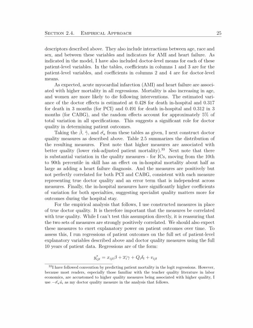
Section 2.4. Empirical Approach 25
descriptors described above. They also include interactions between age, race andsex, and between these variables and indicators for AMI and heart failure. Asindicated in the model, I have also included doctor-level means for each of thesepatient-level variables. In the tables, coefficients in columns 1 and 3 are for thepatient-level variables, and coefficients in columns 2 and 4 are for doctor-levelmeans.
As expected, acute myocardial infarction (AMI) and heart failure are associ-ated with higher mortality in all regressions. Mortality is also increasing in age,and women are more likely to die following interventions. The estimated vari-ance of the doctor effects is estimated at 0.428 for death in-hospital and 0.317for death in 3 months (for PCI) and 0.491 for death in-hospital and 0.312 in 3months (for CABG), and the random effects account for approximately 5% oftotal variation in all specifications. This suggests a significant role for doctorquality in determining patient outcomes.
Taking the β, γ, and σu from these tables as given, I next construct doctorquality measures as described above. Table 2.5 summarizes the distribution ofthe resulting measures. First note that higher measures are associated withbetter quality (lower risk-adjusted patient mortality).33 Next note that thereis substantial variation in the quality measures - for ICs, moving from the 10thto 90th percentile in skill has an effect on in-hospital mortality about half aslarge as adding a heart failure diagnosis. And the measures are positively butnot perfectly correlated for both PCI and CABG, consistent with each measurerepresenting true doctor quality and an error term that is independent acrossmeasures. Finally, the in-hospital measures have significantly higher coefficientsof variation for both specialties, suggesting specialist quality matters more foroutcomes during the hospital stay.
For the empirical analysis that follows, I use constructed measures in placeof true doctor quality. It is therefore important that the measures be correlatedwith true quality. While I can’t test this assumption directly, it is reassuring thatthe two sets of measures are strongly positively correlated. We should also expectthese measures to exert explanatory power on patient outcomes over time. Toassess this, I run regressions of patient outcomes on the full set of patient-levelexplanatory variables described above and doctor quality measures using the full10 years of patient data. Regressions are of the form:
y∗ijt = xijtβ + xiγ +Qiδt + vijt
33I have followed convention by predicting patient mortality in the logit regressions. However,because most readers, especially those familiar with the teacher quality literature in laboreconomics, are accustomed to higher quality measures being associated with higher quality, Iuse −σuui as my doctor quality measure in the analysis that follows.

Section 2.5. Empirical Evidence 26
where Qi is the physician’s quality measure. Table 2.6 displays the coefficientson the doctor quality measure interacted with year dummies (δt). While thepredictive power of the signal declines over time, it is significant at the 1% levelfor all years in all regressions.34 Thus, while some component of the qualitymeasure is likely transitory, these measures also capture a dimension of qualitywhich is persistent.
Table 2.7 compares my preferred quality measures with measures constructedwithout controlling for patient sorting for doctors with high (top quartile) andlow (bottom quartile) levels of patient risk. Columns 1 and 3 give the differencein the doctor’s ordinal rank (with higher quality doctors ranked lower), withthe difference equal to the ranking without controlling for sorting minus themeasure controlling for sorting. Results suggest failing to control for patientsorting significantly penalizes doctors seeing risky patients. These doctors drop42 ranks when controls are added, while doctors with low risk patients gain 85ranks. The difference between the rank movements of these two categories ofdoctors is statistically significant at the 5% level. Results comparing qualitymeasures instead of ranks are in columns 2 and 4. Doctors with risky patientsexperience reductions in quality measures (improvements in measures) around6% of a standard deviation, while doctors with less risky patients experienceincreases in quality measures around 8% of a standard deviation.
2.5 Empirical EvidenceIn this section I use doctor quality measures from the previous section to
determine how physician careers differ by quality, with an eye towards under-standing the importance of learning in the labor market. I begin by analyzingthe careers of ICs. First I test whether low quality ICs are more likely to stopperforming PCI or drop out of cardiology altogether. I determine that a physicianhas dropped out of doing PCI if he has positive PCI years followed by all zeroPCI years. Similarly, I determine that a physician has dropped out of the marketentirely if he has positive procedure years followed by all zero procedure years. Itis important to note that dropping out of the market does not necessarily implydropping out of medical practice. Because I only observe Medicare patients it is
34There is a marked dropoff in the magnitude of coefficients after 1999. Because patientoutcomes for years 1996-1999 are used in constructing the quality measures, this suggests theconstructed quality measures may contain some information that is specific to these calendaryears. To ensure results are not biased by correlations between this transitory component ofquality measures and career outcomes, in Section 2.5 I run robustness checks excluding the firstfour years of data.

Section 2.5. Empirical Evidence 27
possible that these specialists are simply dropping out of private practice.35
Table 2.8 contains results from logit regressions of dropout indicators onquality measures and doctor characteristics. To ease interpretation, the tabledisplays effects of a one standard deviation change in quality on the probabilityof dropping out expressed in percentage points. The top panel includes resultsfor dropping out of performing PCI, and the bottom panel includes results fordropping out of the labor market. The first two columns use the in-hospitaldoctor quality measure, and the third and fourth columns use the in 3 monthsquality measure. Cohort fixed effects are included in columns 2 and 4 to controlfor any quality differences across cohorts that may be driving dropout behavior.Negative coefficients on quality are consistent with learning.
In the top panel, effects are negative and significant at the 5% level in all butone specification. Consistent with the model, lower quality ICs are more likely tostop doing interventional procedures. More precisely, a one standard deviationdecrease in doctor quality increases the likelihood of dropping out of PCI byapproximately one percentage point. Compared with the overall fraction of ICsdropping out of PCI, this is a sizeable effect (a 10% change in the probabilityof dropping out). In the bottom panel, effects are negative in all specificationsbut less precisely measured and smaller in magnitude. Thus, while low qualityICs may choose to stop doing PCI (focusing instead on medical management andtesting or diagnostic angiography), they do not drop out of the labor marketentirely.
As we have seen, the model suggests that dropout behavior should be morepronounced in a declining market. Demand for CT surgeons, especially CABG,was declining during the sample period as a result of the proliferation of baremetal stents (Cutler and Huckman (2003)). Figure 2.1 plots the number ofMedicare patients undergoing PCI, PCI with stent placement and CABG from1996-2005. It is evident from this figure that stents are taking market share awayfrom CABG over time - stent procedures increased their percentage of PCIs byover 200%. And while the overall market for revascularization is growing overtime, the CABG market is declining: CABG procedures decreased by 28% in thesample period, while PCI increased by 75%.
Results from regressions of dropout indicators on quality measures for CTsare in columns 5 through 8 of Table 2.8. Consistent with the model, coefficientsare larger in magnitude and more likely to be statistically significant. Higher
35ICs who stop doing PCI may focus on non-interventional aspects of cardiology, for example,medical management of cardiovascular disease. CT surgeons who stop doing CABG may focuson other thoracic surgeries, for example, carotid endarterectomy, or they may do general surgery.Physicians who drop out of private practice altogether may take salaried positions in HMOgroups or in hospitals. For cardiac specialists, these types of career changes generally involve areduction in pay.
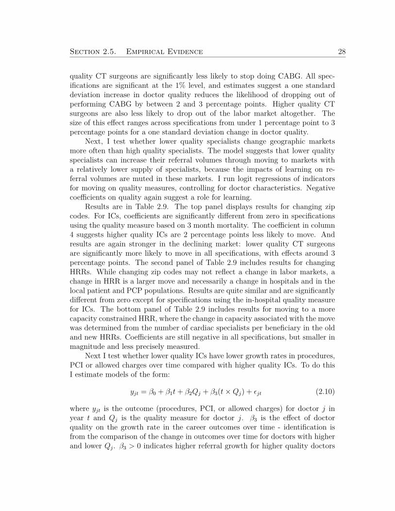
Section 2.5. Empirical Evidence 28
quality CT surgeons are significantly less likely to stop doing CABG. All spec-ifications are significant at the 1% level, and estimates suggest a one standarddeviation increase in doctor quality reduces the likelihood of dropping out ofperforming CABG by between 2 and 3 percentage points. Higher quality CTsurgeons are also less likely to drop out of the labor market altogether. Thesize of this effect ranges across specifications from under 1 percentage point to 3percentage points for a one standard deviation change in doctor quality.
Next, I test whether lower quality specialists change geographic marketsmore often than high quality specialists. The model suggests that lower qualityspecialists can increase their referral volumes through moving to markets witha relatively lower supply of specialists, because the impacts of learning on re-ferral volumes are muted in these markets. I run logit regressions of indicatorsfor moving on quality measures, controlling for doctor characteristics. Negativecoefficients on quality again suggest a role for learning.
Results are in Table 2.9. The top panel displays results for changing zipcodes. For ICs, coefficients are significantly different from zero in specificationsusing the quality measure based on 3 month mortality. The coefficient in column4 suggests higher quality ICs are 2 percentage points less likely to move. Andresults are again stronger in the declining market: lower quality CT surgeonsare significantly more likely to move in all specifications, with effects around 3percentage points. The second panel of Table 2.9 includes results for changingHRRs. While changing zip codes may not reflect a change in labor markets, achange in HRR is a larger move and necessarily a change in hospitals and in thelocal patient and PCP populations. Results are quite similar and are significantlydifferent from zero except for specifications using the in-hospital quality measurefor ICs. The bottom panel of Table 2.9 includes results for moving to a morecapacity constrained HRR, where the change in capacity associated with the movewas determined from the number of cardiac specialists per beneficiary in the oldand new HRRs. Coefficients are still negative in all specifications, but smaller inmagnitude and less precisely measured.
Next I test whether lower quality ICs have lower growth rates in procedures,PCI or allowed charges over time compared with higher quality ICs. To do thisI estimate models of the form:
yjt = β0 + β1t+ β2Qj + β3(t×Qj) + εjt (2.10)
where yjt is the outcome (procedures, PCI, or allowed charges) for doctor j inyear t and Qj is the quality measure for doctor j. β3 is the effect of doctorquality on the growth rate in the career outcomes over time - identification isfrom the comparison of the change in outcomes over time for doctors with higherand lower Qj. β3 > 0 indicates higher referral growth for higher quality doctors

Section 2.5. Empirical Evidence 29
and is consistent with learning by PCPs.Estimates are in Table 2.10. For each quality measure, I run the basic
model (first column), the model using only years 2000-2005 (second column),and a version of the model with a dummy variable indicating the top half ofspecialists in terms of quality (third column). All standard errors are clusteredat the doctor level. The top panel includes results for the procedures outcomevariable; the middle for PCI/CABG; and the bottom for allowed charges. β3 isnot significantly different from zero in any specification for any outcome. This istrue for both ICs and CT surgeons, and for both the estimates rule out increaseslarger than 2% at the 5% significance level (for a one standard deviation increasein doctor quality).
This is an especially strong result, because this specification includes zeroprocedure volumes for dropouts after they have dropped out. However, resultscould still be confounded by specialists’ sorting across HRRs. If lower qualityspecialists locate in more capacity constrained HRRs, they might have higherreferral volumes, biasing results towards zero. To control for this sorting, columns1, 4, 7 and 10 of Table 2.11 include HRR fixed effects. Results are quite similar- even when sorting across markets is taken into account I can rule out effectsof quality larger than 2%. Because we should not expect quality to matter forreferral volumes even within capacity constrained HRRs, next I provide resultsexcluding the lowest capacity third of HRRs.36 Columns 2, 5, 8, and 11 containresults from these regressions. Again there is no divergence in referral volumesby quality.
One might also worry that effects on referral volumes are muted by theinclusion of physicians in large multi-specialty practice groups in the sample,as PCPs in these groups have incentives to refer within-group irrespective ofquality.37 Columns 3, 6, 9, and 12 of Table 2.11 include results from specificationsin which physicians in groups with more than 25 physicians have been dropped.Again coefficients on the interaction between quality and year are not significantlydifferent from zero, and most specifications rule out meaningful effects of qualityon referral volumes.
It is also possible that quality affects referral volumes at points in the distri-bution other than the mean. Table 2.12 presents results from quantile regressions,estimating effects of quality at the 25th, 50th, and 75th percentile of the distri-
36Here HRR capacity is the number of ICs or CT surgeons in my sample billing Medicare ineach HRR divided by the number of Medicare beneficiaries in each HRR.
37I construct a measure of a physician’s group size using the tax numbers physicians billfrom. More specifically, I construct the group size variable using a 20% random sample of theMedicare Part B claims for 2000. I summarize the number of unique doctors in any specialtysubmitting claims from each tax number. Physicians billing from the same tax number areconsidered to be part of the same group.

Section 2.5. Empirical Evidence 30
bution of procedures, PCI/CABG, and charges. Results provide little evidenceof divergence, except perhaps at the 25th percentile of the distribution for CTsurgeons. For this group coefficients on the interaction term in the proceduresregressions are significant and positive, but the sign flips in the regression forCABG and is not significant for charges. Thus, while composition of referralsmay change slightly by quality at the lower tail of the distribution, it does notimpact CT surgeons’ incomes.
Thus far the evidence suggests little effect of learning by PCPs on referralvolumes. However, if reductions in referrals are driving dropout behavior as inthe model we should expect to observe declines in practice volumes for doctorswho drop out prior to their career change. Figure 2.2 and figure 2.3 plot referralvolumes over time for dropouts by the year of dropout and for non-dropouts.Figure 2.2 includes results for ICs and igure 2.3 for CT surgeons. ICs who dropout of the labor market experience declines in total procedures for 3 to 4 yearsprior to their dropout date. ICs who drop out of PCI experience similar declines inPCI before they refocus their careers on non-interventional procedures. Patternsare similar for CT surgeons, but the reduction in referrals appears to be for alonger period of time prior to the dropout date. This is consistent with dropoutbehavior being driven by reductions in referrals by PCPs.
It is also interesting to test whether effects of quality on referral volumes arestronger in areas with lower information costs for PCPs. I restrict the sample ofCT surgeons to those doctors practicing in New York state after the implementa-tion of the CABG report card program. Results, in Table 2.13, suggest that evenin this market referrals of higher and lower quality doctors do not diverge overtime. Coefficients are not significantly different from zero in any specification.Though the results are noisier than in the full sample, most specifications ruleout effects larger than 3%.
The model also predicts that PCPs will increase sorting of patients to spe-cialists based on risk factors over the career. If high ability specialists have arelative advantage at treating high risk patients, then PCPs will sort higher riskpatients to higher quality doctors; if the opposite is true, then PCPs should sorthigher risk patients to lower quality doctors. Because the data supports the no-tion that higher quality doctors have the relative advantage, we expect PCPs tosort higher risk patients to higher quality doctors.38
38To determine how skill in treating risky patients is correlated with overall quality, I ranthe following patient-level random coefficients model, in which the coefficient on patient riskfactors is allowed to vary across doctors:
log pijt1− pijt
= xijtβi + xiγ + σuui
where to simplify computation, xijt is a single-dimensional index of patient risk factors con-

Section 2.5. Empirical Evidence 31
To test predictions for patient risk over the career, I run a model with thesame form as equation 2.10, but with patient risk as the dependent variable. Forsimplicity I use a one dimensional risk index as my patient risk measure.39 Againβ3 > 0 suggests divergence in risk factors, with higher quality specialists receivinghigher risk patients over time.
Results are in Table 2.15. Coefficients on the interaction between year andquality are not significant in any specification. This suggests either PCPs arenot increasing sorting of patients based on quality over time or that this effectis confounded by an opposite effect. For example, if better doctors can increas-ingly avoid risky patients for lifestyle reasons, this would work in the oppositedirection. To avoid this confounding effect, I limit the sample to young cohortsof specialists whose careers are just being established. Results from doctors whobegin practice between 1997-2002 are in Table 2.12.40 For these specialists β3 ispositive and significantly different from zero in most specifications. For ICs, aone standard deviation increase in quality is associated with a 3% of one standarddeviation increase in the risk index. For CT surgeons, estimates range from 2%for regressions using the quality measure based on 3 month mortality to 6% forregressions using the in-hospital quality measure.
Results thus far are consistent with some degree of learning by PCPs. Ininterpreting these results, it is useful to consider how estimates may be affectedby use of the constructed quality measure in place of true quality, which is un-observed. First, consider the possibility that there is classical measurement errorin the quality measure. The covariance between the two quality measures (in-hospital and in 3 months) provides some information on the degree of attenuationto expect. This suggests a reliability ratio of 0.42 for ICs and 0.67 for CT sur-geons, and reliability ratios suggested by comparing quality measures constructedusing different years of patient outcomes are slightly lower.
Next consider impacts on estimates arising from error in the quality mea-sure that is correlated with physician behavior. Recall that nonrandom sort-ing of patients, in a way not captured by controlling for xi, implies that ui =ui + E[ui|vijt, xijt, xi], where ui is true quality. Because we expect riskier pa-tients are likely to sort to better specialists (Glance et al (2008)), we expectE[ui|vijt, xijt] < 0(> 0) for higher (lower) quality specialists. Intuitively, higher
structed from the β estimated in the previous section. The coefficient of interest is the covariancebetween ui and βi. A negative covariance is consistent with better doctors having a relativeadvantage, and in fact this is what I find. These results are available upon request.
39This index is constructed as mean predicted mortality based on patient risk characteristics,where the prediction uses the coefficients estimated in the patient-level regressions in Section2.3.
40These are doctors whose graduation years are consistent with starting practice in the periodand whose dates of beginning practice I can verify by observing zero procedure years precedingpositive procedure years.

Section 2.6. Conclusion 32
quality physicians are penalized for treating riskier patients - their quality mea-sure is biased downwards. The opposite is true for lower quality specialists, whosee less risky patients. And we expect this error in the quality measure to bepositively correlated with dropout behavior since higher quality doctors are lesslikely to drop out, resulting in positive bias (towards zero). For the analysis ofmoving behavior the bias is also positive (towards zero), and for the analysisof procedure volumes, where we expect a positive coefficient, the bias is nega-tive (towards zero). Therefore, if anything, the results presented in this sectionunderestimate the true effect of quality on careers.
Results may also be affected by the fact that we observe only Medicarepatients. If the fraction of Medicare referrals accepted by specialists or specialistparticipation in Medicare is unrelated to quality, then this is a case of classicalmeasurement error in the dependent variable. If, on the other hand, betterdoctors are more likely to drop out of Medicare, then this could bias results ofthe dropout analysis towards zero. However, the large majority (approximately90%) of physicians in the U.S. are contracted with Medicare, suggesting this effectis likely small. It may also be the case that doctors are able to differentially selectpatients on insurance status over the course of their career. If we think betterquality doctors may select away from Medicare patients over time, then thiswould bias the analysis of patient and procedure volumes downwards. However,because Medicare patients make up such a large fraction of cardiac specialists’patients, this is an unlikely scenario. Considering all the sources of bias together,the estimates presented in this section likely give a lower bound on actual effects.
2.6 ConclusionThis chapter examines the the role of market learning about relative quality
(or ability) in the labor market for medical specialists. Adapting models of em-ployer learning from labor economics, I model the referral relationship betweenPCPs and specialists. The model makes predictions for specialist careers andilluminates quality incentives arising from this relationship. I then test the pre-dictions of the model using confidential Medicare claims data from the universeof cardiac specialists in the U.S.
The empirical evidence is consistent with some degree of learning by PCPs.Lower quality interventional cardiologists are more likely to stop doing PCI. Theyare also more likely to move their practice across geographic markets to avoid theeffects of reputation on referrals. Moreover, the effects of quality on moving anddropout behavior are stronger for CT surgeons, for whom labor demand wasdeclining over the sample period. Lower quality CT surgeons are more likely tostop doing CABG, to change geographic markets, and even to drop out of the

Section 2.6. Conclusion 33
labor market altogether. Also consistent with the model, PCPs increasingly sortpatients to specialists based on their risk characteristics over time. As specialists’quality becomes known in early careers, PCPs increasingly send risky patients tospecialists with a relative advantage at handling patient risk.
This chapter also presents a new methodology for measuring doctor qualityusing data on patient outcomes. My quality measure controls for nonrandomsorting of patients to higher and lower quality specialists based on risk character-istics. Failing to control for this type of sorting substantially penalizes specialistsseeing relatively risky patients. This finding has implications for report card de-sign and other programs aimed at measuring and evaluating providers based onquality. A similar methodology could also be applied to measure quality in othercontexts. For example, one could construct a measure of teacher quality basedon the likelihood that students drop out, controlling for sorting of students toteachers on observable characteristics.
This chapter also shows that learning by PCPs does not result in divergencein practice volumes over time by quality. This suggests that financial impacts oflearning on specialists are small conditional on staying locally in practice, perhapsbecause moving and dropout behavior mitigate effects on those who remain.
These findings have implications for patient welfare. Low quality specialistsstopping doing PCI or stopping practicing altogether is welfare-improving assum-ing adequate physician supply. Further, the sorting of higher risk cases to betterphysicians, who have a comparative advantage at treating these cases, increasespatient survival. Finally, the fact that lower quality specialists are more likely tomove to capacity constrained areas has distributional consequences, as patientsin these areas may receive lower quality care.

Section 2.7. Figures 34
2.7 Figures
Figure 2.1: CABG, PCI and Stent Claims Over Time
0
50,000
100,000
150,000
200,000
250,000
300,000
350,000
400,000
450,000
1996 1997 1998 1999 2000 2001 2002 2003 2004 2005Year
Num
ber o
f Cla
ims CABG
PCIStent
Plot points are the total number of Medicare Part B claims involving each procedure(PCI (of any kind), PCI with stent placement, and CABG.) Duplicate and deniedclaims have been excluded.

Section 2.7. Figures 35
Figure 2.2: Time Trends in Referral Volumes by Dropout Status - ICs
Total Claims by Dropout Status
020
0040
0060
0080
00T
otal
Pro
cedu
res
1996 1998 2000 2002 2004 2006Year
Dropouts 201 Dropouts 2002Dropouts 2003 Dropouts 2004Dropouts 2005 Non−Dropouts
Total PCI Claims by PCI Dropout Status
020
4060
80T
otal
PC
I Pro
cedu
res
1996 1998 2000 2002 2004 2006Year
Dropouts 2001 Dropouts 2002Dropouts 2003 Dropouts 2004Dropouts 2005 Non−Dropouts
Procedures Over Time for PCI Dropouts
Figures display referral volumes over time for dropouts and non-dropouts. For dropouts, volumes are plotted separately for eachdropout cohort, with the cohort defined by the year they drop out.The top panel displays results for dropping out of practice and thebottom for dropping out of performing PCI.

Section 2.7. Figures 36
Figure 2.3: Time Trends in Referral Volumes by Dropout Status - CT Surgeons
Total Claims by Dropout Status
020
040
060
0T
otal
Pro
cedu
res
1996 1998 2000 2002 2004 2006Year
Dropouts 201 Dropouts 2002Dropouts 2003 Dropouts 2004Dropouts 2005 Non−Dropouts
Total CABG Claims by CABG Dropout Status
020
4060
8010
0T
otal
CA
BG
Pro
cedu
res
1996 1998 2000 2002 2004 2006Year
Dropouts 2001 Dropouts 2002Dropouts 2003 Dropouts 2004Dropouts 2005 Non−Dropouts
Figures display referral volumes over time for dropouts and non-dropouts. For dropouts, volumes are plotted separately for eachdropout cohort, with the cohort defined by the year they drop out.The top panel displays results for dropping out of practice and thebottom for dropping out of performing CABG.

Section 2.8. Tables 37
2.8 Tables
Table 2.1: Physician Summary StatisticsICs CT Surgeons
Mean Std. Dev. Mean Std. Dev.
Physician characteristicsForeign medical school (%) 23 42 17 37Prestigious medical school (%) 15 36 20 40HRR beneficiaries 148083 105283 149216 107233HRR spending level 6438 1358 6496 1382Experience 11.2 6.7 14.7 38.1Practice volumeProcedures 5500 3636 558 742PCI / CABG 63 46 76 45Allowed Charges 411126 265225 260584 149627Patients 1166 676 229 205Case mix - procedures% PCI/CABG 4.0 5.6 28.1 21.6% Other Procedures 6.6 7.8 26.6 17.5% Testing 33.8 15.9 5.4 13.0% Lab 5.8 8.0 0.42 3.7% E&M 36.7 13.4 39.4 21.9Case mix - charges% PCI/CABG 20.0 13.3 43.6 21.7% Other Procedures 15.2 8.8 33.9 19.8% Testing 22.0 12.6 2.5 8.2% Lab 1.0 1.9 0.11 2.11% E&M 23.5 10.4 20.0 21.4Case mix - location% Office 39 19 17 15% Inpatient 46 15 77 16% Outpatient 13 8.6 4.3 7.2Practice moves% PCI/CABG Dropouts 10 30 22 42% Dropouts 2.7 16 16 37% Movers (Across Zip Codes) 17.7 38.2 25.5 43.6N 4237 2838Sample includes ICs and CT surgeons performing at least 30 procedures(PCI / CABG) by 1999. Statistics are calculated from annual measuresfor years 1996-2005.

Section 2.8. Tables 38
Table 2.2: Patient Level Summary StatisticsPCI Sample CABG Sample
Mean Std. Dev. Mean Std. Dev.
Outcome Measures (%)Death in hospital 1.4 12.0 3.0 17.0Death in 3 months 4.0 20.0 4.7 21.2Risk Characteristics (%)AMI 20.0 40.0 5.0 21.9Heart Failure 5.4 23.0 2.6 15.8Peripheral Vasc Disease 1.7 13.0 1.6 12.5Cerebrovascular Disease 0.59 7.7 1.4 11.9Chronic Pulmonary Disease 0.82 9.0 0.78 8.8Rheumatoid Arthritis 0.016 1.3 0.017 1.3Diabetes w/o Complications 1.5 12.0 1.4 11.6Renal Disease 0.29 5.3 0.29 5.4DemographicsDisability (%) 9.4 29.0 5.1 22.0End stage renal disease (%) 1.0 10.0 0.65 8.0Age 72.0 8.2 72.7 7.2Female (%) 43.0 49.0 36.4 48.1Black (%) 5.3 22.0 4.1 19.9Asian (%) 0.57 7.5 0.72 8.4Hispanic (%) 1.4 12.0 1.6 12.6Zipcode income 21,163 9,031 21,174 9,062Procedure Information (%)Angioplasty Only 41.4 49.3Stent 54.5 49.8Count of Vessels 121 47.8Left Circumflex Artery 12.7 33.3Left Anterior Descending 17.8 38.2Right Coronary Artery 16.7 37.3Diagnostic Cath 43.7 49.6Reoperation 10.0 30.0Artery 68.5 46.5Vein 28.6 45.2Artery & Vein 62.9 48.3Number Vessels 2.65 1.08Number Arteries 1.13 0.45N 1,067,018 1,019,770Sample includes all claims involving PCI or CABG in 1996-1999,as determined from procedure codes. Excludes duplicate and de-nied claims.

Section 2.8. Tables 39
Table 2.3: Coefficients from Correlated Random Effects Logits - PCI Sample
In hospital In 3 monthsxijt xi xijt xi
Risk CharacteristicsAMI 1.570 -1.703 0.923 -1.357
(0.025) (0.60) (0.015) (0.38)Heart Failure 0.695 -0.0314 1.073 -0.164
(0.040) (0.31) (0.022) (0.20)Periph Vasc Disease 0.0589 0.942 0.347 0.287
(0.069) (0.64) (0.036) (0.43)Chronic Pulmonary Disease 0.130 0.787 0.497 -0.131
(0.085) (0.67) (0.046) (0.45)Diabetes w/o Complications -0.478 -1.388 -0.0146 -1.264
(0.087) (0.47) (0.044) (0.31)Renal Disease 0.775 2.095 0.858 -0.368
(0.10) (1.72) (0.060) (1.13)DemographicsDisability 0.406 -0.0293 0.445 0.816
(0.053) (0.62) (0.030) (0.40)End stage renal disease 1.297 1.166 1.635 2.824
(0.079) (1.11) (0.042) (0.70)Age -0.0238 -0.513 -0.0203 -0.523
(0.013) (0.16) (0.0077) (0.11)Age squared 0.000605 0.00372 0.000590 0.00394
(0.000088) (0.0011) (0.000051) (0.00072)Female 0.809 1.013 0.959 -0.244
(0.16) (2.37) (0.095) (1.53)Black 0.0225 4.037 0.227 2.259
(0.30) (3.36) (0.16) (2.11)Asian 0.0592 -0.699 0.0737 -0.147
(0.11) (0.55) (0.066) (0.33)Hispanic 0.106 0.0892 0.0569 0.307
(0.072) (0.32) (0.044) (0.21)Age*Female -0.00651 -0.0108 -0.0120 0.00459
(0.0021) (0.032) (0.0013) (0.021)Black*Female -0.0497 -1.814 0.0105 -1.076
(0.081) (1.10) (0.044) (0.69)Age*Black -0.000574 -0.0380 -0.00193 -0.0159
(0.0041) (0.049) (0.0022) (0.030)AMI*Black -0.195** -0.261 -0.00397 0.112
(0.079) (1.03) (0.045) (0.66)Heart Failure*Black -0.113 -1.725 -0.264 -1.147
(0.12) (1.49) (0.064) (0.91)AMI*Female -0.0402 -0.335 0.0683 0.481
(0.033) (0.67) (0.021) (0.44)Heart Failure*Female -0.205 1.548 -0.184 0.948
(0.054) (1.19) (0.031) (0.76)Zipcode Income -0.00000239 -0.0000194 -0.00000435 -0.00000453
(0.0000011) (0.0000032) (0.00000068) (0.0000020)Procedure InformationAngioplasty Only 0.534 -0.409 0.322 -0.551
(0.054) (0.22) (0.030) (0.14)Stent -0.0181 -0.0475 0.0908 -0.303
(0.054) (0.23) (0.030) (0.15)Count of Vessels -0.108 0.201 0.0225 0.0715
(0.020) (0.090) (0.011) (0.058)Left Circumflex Artery -0.0558 -0.248 0.0340 -0.346
(0.030) (0.25) (0.017) (0.17)Left Anterior Descending 0.155 0.444 0.146 0.408
(0.025) (0.22) (0.015) (0.14)Right Coronary Artery -0.0901 0.00419 -0.100 -0.0544

Section 2.8. Tables 40
Table 2.3: (continued)
In hospital In 3 monthsxijt xi xijt xi
(0.027) (0.24) (0.016) (0.15)Diagnostic Cath 0.117 0.193 0.0458 -0.0104
(0.019) (0.055) (0.011) (0.035)Sigmau 0.428 0.317
(0.0137) (0.0082)Year Dummies Yes YesPseudo R-squared 0.088 0.059N 1,067,018 1,067,018Sample includes any claim involving PCI in 1996-1999, as identified from procedure codes.Excludes denied and duplicate claims. Results are from logit regressions of patient mor-tality on the listed explanatory variables, with doctor level random effects. Coefficientsare presented. Standard errors are in parentheses.

Section 2.8. Tables 41
Table 2.4: Coefficients from Correlated Random Effects Logits - CABG Sample
In hospital In 3 monthsxijt xi xijt xi
Risk CharacteristicsAMI 0.678 -1.547 0.279 -0.596
(0.033) (0.47) (0.028) (0.33)Heart Failure 0.980 -1.588 0.644 -0.0456
(0.037) (0.79) (0.032) (0.55)Periph Vasc Disease 1.137 -1.154 0.472 -0.301
(0.032) (0.29) (0.032) (0.20)Chronic Pulmonary Disease -0.0942 0.583 0.653 -0.948
(0.074) (0.67) (0.045) (0.48)Diabetes w/o Complications -0.0469 -1.405 -0.0493 -0.500
(0.057) (0.46) (0.045) (0.32)Renal Disease 0.614 4.424 0.917 3.623
(0.077) (1.75) (0.057) (1.22)DemographicsDisability 0.376 -1.166 0.372 1.783
(0.035) (0.76) (0.031) (0.53)End stage renal disease 1.165 2.512 1.427 1.896
(0.054) (1.46) (0.043) (1.02)Age -0.00518 -0.103 -0.00218 -0.252
(0.010) (0.22) (0.0088) (0.15)Age squared 0.000305 -0.0000290 0.000464 0.00193
(0.000068) (0.0015) (0.000058) (0.0010)Female 0.790 -6.534 1.723 -0.775
(0.12) (3.03) (0.10) (2.11)Black 0.857 6.381 0.703 0.303
(0.22) (4.76) (0.18) (3.27)Asian 0.332 -0.614 0.0535 0.532
(0.064) (0.45) (0.054) (0.31)Hispanic 0.0582 1.082 0.0667 0.901
(0.048) (0.27) (0.038) (0.19)Age*Female -0.00525 0.0884 -0.0208 0.0176
(0.0016) (0.041) (0.0013) (0.029)Black*Female -0.471 -2.632 -0.134 -2.045
(0.057) (1.35) (0.045) (0.94)Age*Black -0.00716 -0.0695 -0.00669 0.0194
(0.0031) (0.067) (0.0025) (0.046)AMI*Black -0.210 3.239 -0.213 0.589
(0.11) (0.89) (0.10) (0.68)Heart Failure*Black -0.152 -2.519 -0.274 3.458
(0.12) (2.91) (0.11) (1.99)AMI*Female 0.153 0.0991 0.0627 -0.126
(0.045) (1.27) (0.040) (0.89)Heart Failure*Female -0.192 1.822 0.0192 -1.761
(0.053) (1.77) (0.046) (1.23)Zipcode Income -0.00000127 -0.00000179 -0.00000437 0.00000311
(0.00000081) (0.0000033) (0.00000065) (0.0000023)Procedure InformationReoperation 0.932 -0.126 0.198 0.960
(0.017) (0.27) (0.017) (0.18)Artery 0.206 2.026 -0.231 1.538
(0.072) (0.84) (0.061) (0.58)Vein 0.194 -1.050 0.934 -0.335
(0.24) (4.57) (0.22) (3.43)Artery & Vein -0.192 -0.556 0.564 -0.226
(0.24) (4.59) (0.22) (3.45)Sigmau 0.491 0.312
(0.0104) (0.0077)Number of vessel dummies Yes Yes

Section 2.8. Tables 42
Table 2.4: (continued)
In hospital In 3 monthsxijt xi xijt xi
Year Dummies Yes YesPseudo R-squared 0.057 0.039N 1,019,770 1,019,770Sample includes any claim involving CABG in 1996-1999, as identified from procedurecodes. Excludes denied and duplicate claims. Results are from logit regressions of patientmortality on the listed explanatory variables, with doctor level random effects. Coeffi-cients are presented. Standard errors are in parentheses.

Section 2.8. Tables 43
Tabl
e2.
5:D
octo
rQ
ualit
yM
easu
res
ICs
CT
Surg
eons
Dist
ribut
ion
ofm
easu
res:
Inho
spita
lIn
3m
onth
sIn
hosp
ital
In3
mon
ths
10th
perc
entil
e-0
.15
-0.0
86-0
.25
-0.0
9325
thpe
rcen
tile
-0.0
67-0
.039
-0.1
3-0
.044
50th
perc
entil
e0.
013
0.00
470.
0076
0.00
1975
thpe
rcen
tile
0.07
80.
044
0.13
0.04
990
thpe
rcen
tile
0.12
0.07
80.
160.
088
90-1
0ga
p0.
270.
160.
410.
18
Std.
Dev
0.11
0.06
40.
190.
071
Coe
ffici
ent
ofva
riatio
n7.
81.
66.
41.
5C
orre
latio
n0.
420.
27N
4,23
72,
838
Sam
ple
incl
udes
ICs
and
CT
surg
eons
perfo
rmin
gat
leas
t30
proc
edur
es(P
CI/
CA
BG)
by19
99.
Col
umns
(1)
and
(3)
sum
mar
ize
doct
orqu
ality
mea
sure
sba
sed
onth
ede
ath
in-h
ospi
talp
atie
ntou
tcom
e(C
olum
n(1
)su
mm
ariz
esm
easu
res
for
ICs
and
Col
umn
(3)
for
CT
surg
eons
).C
olum
ns(2
)an
d(4
)co
ntai
nm
easu
res
base
don
patie
ntm
orta
lity
in3
mon
ths
but
not
in-h
ospi
tal.
Qua
lity
mea
sure
sar
eco
nstr
ucte
din
atw
o-st
eppr
oced
ure
asde
scrib
edin
Sect
ion
2.3.

Section 2.8. Tables 44
Table 2.6: Doctor Quality Measures Over Time
PCI Sample CABG SampleIn hospital In 3 months In hospital In 3 months
1996 5.451 6.579 3.352 6.275(0.15) (0.16) (0.063) (0.13)
1997 5.666 6.446 3.349 6.268(0.15) (0.16) (0.062) (0.13)
1998 5.536 6.421 2.448 4.417(0.15) (0.15) (0.064) (0.14)
1999 5.489 6.396 2.385 4.501(0.15) (0.15) (0.066) (0.14)
2000 2.061 2.487 1.320 1.628(0.16) (0.15) (0.070) (0.14)
2001 1.927 2.289 1.156 1.852(0.16) (0.15) (0.074) (0.14)
2002 1.628 2.438 1.288 1.510(0.17) (0.15) (0.078) (0.15)
2003 1.509 1.506 1.046 1.680(0.17) (0.15) (0.081) (0.16)
2004 1.602 1.791 0.912 1.526(0.18) (0.16) (0.083) (0.16)
2005 1.123 2.109 0.674 1.644(0.19) (0.16) (0.092) (0.17)
Constant 19.43 16.77 8.485 6.224(5.32) (3.28) (5.43) (4.42)
Observations 2,656,471 2,656,471 2,112,678 2,112,678
Standard errors are in parentheses. Results are from logit regressions ofpatient mortality on doctor quality interacted with year dummies:
y∗ijt = xijtβ + xiγ +Qiδt + vijt
where xijt is the full set of patient-level explanatory variables in Tables4 and 5. Coefficients displayed are δt. Coefficients in Column (1) arefrom regressions run on the sample of patients undergoing PCI from1996-2005 using the in-hospital mortality quality measure; Column (2)the PCI sample using the in 3 months quality measure; Column (3)the sample of patients undergoing CABG from 1996-2005 using the in-hospital mortality quality measure; and Column (4) the CABG sampleusing the in 3 months quality measure.

Section 2.8. Tables 45
Tabl
e2.
7:D
octo
rQ
ualit
yM
easu
res
Con
trol
ling
for
Patie
ntSo
rtin
g
Inho
spita
lIn
3m
onth
sD
iffer
ence
Diff
eren
ceD
iffer
ence
Diff
eren
cein
Ran
kin
Mea
sure
inR
ank
inM
easu
reH
igh
Risk
Patie
nts
(N=
998)
-42.
17-0
.056
-82.
27-0
.122
(10.
78)
(0.0
11)
(15.
51)
(0.0
18)
Low
Risk
Patie
nts
(N=
999)
85.4
70.
078
104.
800.
116
(6.7
8)(0
.007
)(9
.49)
(0.0
13)
T-s
tatis
tic(d
iffer
ence
inm
eans
)-1
0.03
-10.
19-1
0.29
-10.
71St
anda
rder
rors
inpa
rent
hese
s.Ta
ble
com
pare
sm
ypr
efer
red
qual
itym
easu
res
with
mea
sure
scon
stru
cted
with
outc
ontr
ollin
gfo
rpat
ient
sort
ing
ford
octo
rsw
ithpa
tient
sin
the
top
and
bott
omris
kqu
artil
es.
Col
umns
(1)
and
(3)
give
the
diffe
renc
ein
the
doct
or’s
ordi
nalr
ank
(with
high
erqu
ality
doct
ors
rank
edlo
wer)
.T
hedi
ffere
nce
isth
era
nkin
gw
ithou
tcon
trol
ling
fors
ortin
gm
inus
the
mea
sure
cont
rolli
ngfo
rsor
ting.
Col
umns
(2)
and
(4)
give
the
diffe
renc
ein
the
mea
sure
s,ex
pres
sed
asa
fract
ion
ofon
est
anda
rdde
viat
ion
ofea
chm
easu
re.

Section 2.8. Tables 46
Table 2.8: Dropout Analysis
ICs CT Surgeons
In hospital In 3 months In hospital In 3 months
PCI Dropout (1) (2) (3) (4) (5) (6) (7) (8)
Doctor Quality -1.05 -0.91 -0.79 -1.01 -3.21 -2.00 -2.71 -2.00(0.47) (0.43) (0.43) (0.39) (0.77) (0.72) (0.77) (0.73)
Foreign School -2.58 -3.66 -2.66 -3.71 5.57 -4.83 5.32 -4.92(1.07) (0.89) (1.06) (0.88) (2.34) (1.82) (2.32) (1.81)
Prestigious School 0.01 -1.38 -0.06 -1.45 3.08 -0.52 3.26 -0.32(1.29) (1.04) (1.29) (1.03) (2.10) (1.87) (2.11) (1.88)
HRR Size - Benes -3.91 -0.09 -4.58 -0.45 -7.79 11.69 -9.48 10.70(10.84) (9.82) (10.84) (9.77) (18.55) (17.37) (18.66) (17.48)
HRR Size - Reimb -0.39 -0.14 -0.41 -0.17 -2.83 -3.61 -2.97 -3.70(0.55) (0.51) (0.55) (0.51) (0.96) (0.93) (0.97) (0.94)
Cohort fixed effects Yes Yes Yes YesPseudo R-squared 0.011 0.15 0.011 0.15 0.014 0.18 0.010 0.18
Dropout
Doctor Quality -0.33 -0.20 -0.28 -0.27 -2.64 -1.22 -1.88 -1.08(0.25) (0.17) (0.25) (0.16) (0.67) (0.54) (0.67) (0.56)
Foreign School 0.19 (0.27) 0.16 (0.28) 5.28 (3.28) 5.08 (3.33)(0.62) (0.36) (0.62) (0.35) (2.11) (1.31) (2.10) (1.31)
Prestigious School 1.07 0.22 1.04 0.20 2.73 (0.53) 2.84 (0.43)(0.78) (0.44) (0.78) (0.43) (1.87) (1.39) (1.88) (1.40)
HRR Size - Benes 11.58 8.26 11.37 8.16 (6.47) 11.15 (7.66) 10.33(5.56) (3.78) (5.55) (3.72) (16.30) (13.08) (16.41) (13.19)
HRR Size - Reimb (0.77) (0.46) (0.78) (0.47) (2.36) (2.83) (2.47) (2.89)(0.31) (0.22) (0.31) (0.21) (0.84) (0.70) (0.86) (0.71)
Cohort fixed effects Yes Yes Yes YesPseudo R-squared 0.0047 0.086 0.0041 0.087 0.012 0.14 0.010 0.14N 4228 4221 4228 4221 2815 2815 2815 2815Table displays results from logit regressions of dropout indicators on quality measures anddoctor characteristics. The top panel is for regressions using indicators for dropping out ofPCI or CABG, and the bottom panel uses indicators for stopping billing Medicare altogether.In Columns (1), (2), (5), and (6) “Doctor Quality” is the in-hospital quality measure. In theremaining columns “Doctor Quality” is based on 3 month mortality. Effects are for a onestandard deviation change in X on the probability of dropping out (in percentage points). Fordummy variables the effect is for a discrete change of from 0 to 1. Robust standard errors arein parentheses.

Section 2.8. Tables 47
Table 2.9: Moves AnalysisICs CT Surgeons
In hospital In 3 months In hospital In 3 months
Change in zip code (1) (2) (3) (4) (5) (6) (7) (8)
Doctor Quality -0.93 -0.67 -2.51 -1.98 -2.89 -3.69 -2.62 -3.04(0.58) (0.57) (0.54) (0.54) (0.81) (0.83) (0.82) (0.82)
Foreign School 3.37 5.35 3.46 5.34 -6.97 2.66 -7.15 2.29(1.52) (1.53) (1.52) (1.53) (2.11) (2.67) (2.10) (2.65)
Prestigious School 1.32 1.93 1.24 1.85 -1.95 0.33 -1.78 0.50(1.75) (1.75) (1.74) (1.74) (2.05) (2.14) (2.05) (2.14)
HRR Size - Benes -47.48 -52.22 -47.06 -51.69 -31.31 -51.36 -32.92 -54.05(13.58) (13.06) (13.48) (13.06) (19.41) (19.62) (19.41) (19.62)
HRR Size - Reimb 0.34 0.27 0.27 0.21 0.53 0.93 0.42 0.80(0.70) (0.69) (0.71) (0.70) (0.95) (0.96) (0.95) (0.97)
Pseudo R-squared 0.0055 0.057 0.0098 0.060 0.0082 0.082 0.0075 0.080
Change in HRR
Doctor Quality -0.82 -0.63 -1.68 -1.22 -2.57 -2.89 -2.79 -2.82(0.52) (0.51) (0.49) (0.48) (0.92) (0.90) (0.92) (0.91)
Foreign School 1.53 2.95 1.56 2.91 -8.20 0.16 -8.34 -0.11(1.37) (1.37) (1.36) (1.36) (2.34) (2.97) (2.33) (2.95)
Prestigious School 2.28 2.91 2.21 2.85 -3.71 -1.65 -3.54 -1.54(1.63) (1.61) (1.62) (1.61) (2.26) (2.31) (2.27) (2.31)
HRR Size - Benes -39.06 -42.22 -38.95 -42.11 -17.16 -36.78 -19.30 -39.14(12.32) (11.90) (12.21) (11.79) (21.77) (21.88) (21.77) (21.98)
HRR Size - Reimb 0.59 0.51 0.54 0.48 0.21 0.70 0.04 0.55(0.64) (0.62) (0.64) (0.62) (1.07) (1.07) (1.08) (1.08)
Pseudo R-squared 0.0045 0.044 0.0069 0.046 0.0091 0.078 0.0096 0.078
Change to constrained HRR
Doctor Quality -0.41 -0.32 -0.95 -0.67 -1.66 -1.72 -0.84 -0.74(0.37) (0.35) (0.35) (0.34) (0.68) (0.69) (0.68) (0.69)
Foreign School -0.24 0.68 -0.22 0.66 -3.98 -0.51 -4.09 -0.69(0.97) (0.96) (0.96) (0.96) (1.75) (2.27) (1.75) (2.26)
Prestigious School 0.50 0.91 0.46 0.87 -3.70 -2.94 -3.73 -3.03(1.17) (1.13) (1.16) (1.13) (1.61) (1.69) (1.63) (1.69)
HRR Size - Benes -22.64 -23.69 -22.32 -23.58 5.93 -0.35 5.13 -1.21(9.17) (8.64) (9.05) (8.57) (17.26) (17.80) (17.37) (18.02)
HRR Size - Reimb 0.71 0.62 0.68 0.60 -1.17 -1.05 -1.21 -1.06(0.45) (0.43) (0.45) (0.43) (0.84) (0.87) (0.84) (0.87)
Cohort fixed effects Yes Yes Yes YesPseudo R-squared 0.0034 0.045 0.0058 0.046 0.010 0.045 0.0076 0.041N 4228 4046 4228 4046 2120 1985 2120 1985Table displays results from logit regressions of indicators for moving on quality measures and doctorcharacteristics. The top panel is for regressions using indicators for changing zip codes, the middlepanel for changing HRRs, and the bottom panel for moving to a more capacity constrained HRR. InColumns (1), (2), (5), and (6) “Doctor Quality” is the in-hospital quality measure. In the remainingcolumns “Doctor Quality” is based on 3 month mortality. Effects are for a one standard deviationchange in X on the probability of dropping out (in percentage points). For dummy variables theeffect is for a discrete change of from 0 to 1. Robust standard errors are in parentheses.

Section 2.8. Tables 48
Tabl
e2.
10:
Ana
lysis
ofR
efer
ralV
olum
esIC
sC
TSu
rgeo
ns
Inho
spit
alIn
3m
onth
sIn
hosp
ital
In3
mon
ths
Pro
cedu
res
(1)
(2)
(3)
(4)
(5)
(6)
(7)
(8)
(9)
(10)
(11)
(12)
Qua
lity
0.88
0.59
6.99
7.17
-0.9
7-4
.33
-1.8
3-3
.32
(1.2
0)(1
.37)
(1.0
0)(1
.11)
(4.3
6)(5
.59)
(1.9
3)(1
.99)
Qua
lity*
Yea
r0.
045
-0.0
580.
0070
-0.1
60.
971.
640.
015
0.38
(0.1
6)(0
.23)
(0.1
5)(0
.20)
(0.6
0)(1
.04)
(0.2
8)(0
.39)
Yea
r4.
914.
874.
894.
914.
874.
910.
241.
900.
490.
241.
901.
29(0
.14)
(0.1
9)(0
.28)
(0.1
4)(0
.19)
(0.2
7)(0
.40)
(0.5
9)(0
.90)
(0.4
0)(0
.60)
(0.9
4)R
-squ
ared
0.07
0.07
0.05
0.07
0.07
0.06
0.00
0.02
0.01
0.00
0.02
0.01
PC
I/
CA
BG
Qua
lity
6.08
7.13
2.01
3.12
11.8
510
.83
7.98
7.51
(1.5
5)(1
.73)
(1.2
0)(1
.43)
(1.0
5)(1
.21)
(1.0
3)(1
.18)
Qua
lity*
Yea
r0.
26-0
.062
-0.0
050
-0.2
1-0
.29
-0.4
4-0
.10
-0.2
6(0
.21)
(0.2
7)(0
.17)
(0.2
4)(0
.19)
(0.2
4)(0
.18)
(0.2
3)Y
ear
2.35
0.78
0.58
2.35
0.78
0.60
-6.7
9-7
.01
-6.8
1-6
.79
-7.0
1-6
.66
(0.1
6)(0
.22)
(0.3
2)(0
.16)
(0.2
2)(0
.32)
(0.2
0)(0
.24)
(0.3
0)(0
.20)
(0.2
4)(0
.31)
R-s
quar
ed0.
010.
030.
000.
010.
020.
000.
100.
130.
050.
080.
120.
04
Allo
wed
Cha
rges
Qua
lity
2.22
2.36
6.52
7.16
7.20
5.72
3.64
2.72
(1.1
9)(1
.32)
(1.0
1)(1
.15)
(1.1
5)(1
.26)
(1.0
8)(1
.14)
Qua
lity*
Yea
r-0
.03
-0.3
10.
12-0
.15
0.00
-0.0
2-0
.14
-0.1
0(0
.18)
(0.2
5)(0
.17)
(0.2
4)(0
.18)
(0.2
3)(0
.17)
(0.2
1)Y
ear
5.57
6.04
5.88
5.57
6.04
6.05
-4.9
4-3
.12
-3.3
8-4
.94
-3.1
2-2
.91
(0.1
6)(0
.22)
(0.3
2)(0
.16)
(0.2
2)(0
.32)
(0.1
8)(0
.21)
(0.2
9)(0
.18)
(0.2
1)(0
.31)
R-s
quar
ed0.
070.
070.
050.
080.
080.
060.
060.
100.
020.
050.
100.
01O
bser
vati
ons
4228
025
368
2536
842
280
2536
825
368
2815
016
890
1689
028
150
1689
016
890
Tabl
edi
spla
ysre
sult
sfr
omre
gres
sion
sof
refe
rral
volu
mes
onsp
ecia
list
qual
ity,
year
(ran
ging
from
0in
1996
to10
in20
05),
aqu
ality
-yea
rin
tera
ctio
nan
ddo
ctor
char
acte
rist
ics.
Inth
eto
ppa
nel
the
left
hand
side
vari
able
ispr
oced
ures
(tot
alcl
aim
s),
inth
em
iddl
epa
nel
itis
tota
lcl
aim
sfo
rP
CI
orC
AB
G,
and
inth
ebo
ttom
pane
lit
isM
edic
are
allo
wed
char
ges.
InC
olum
ns(1
)-(3
)an
d(7
)-(9
)“D
octo
rQ
ualit
y”is
the
in-h
ospi
tal
qual
itym
easu
re.
Inth
ere
mai
ning
colu
mns
“Doc
tor
Qua
lity”
isba
sed
on3
mon
thm
orta
lity.
Hig
hQ
ualit
yis
adu
mm
yva
riab
leeq
ual
toon
efo
rdo
ctor
sin
the
top
half
ofth
equ
ality
dist
ribu
tion
.E
ffect
sar
efo
ra
one
stan
dard
devi
atio
nch
ange
inX
onY
(exp
ress
edas
ape
rcen
tage
ofY
).Fo
rdu
mm
yva
riab
les
the
effec
tis
for
ach
ange
from
0to
1.St
anda
rder
rors
,cl
uste
red
atth
edo
ctor
leve
l,ar
ein
pare
nthe
ses.
Reg
ress
ions
incl
ude
coho
rtfix
edeff
ects
.C
olum
ns(1
),(4
),(7
),an
d(1
0)in
clud
ere
sult
sfo
rth
efu
lllo
ngit
udin
alsa
mpl
e.T
here
mai
ning
colu
mns
incl
ude
resu
lts
usin
gon
lyye
ars
2000
-200
5.

Section 2.8. Tables 49
Tabl
e2.
11:
Ana
lysis
ofR
efer
ralV
olum
es-R
obus
tnes
sIC
sC
TSu
rgeo
ns
Inho
spit
alIn
3m
onth
sIn
hosp
ital
In3
mon
ths
Pro
cedu
res
(1)
(2)
(3)
(4)
(5)
(6)
(7)
(8)
(9)
(10)
(11)
(12)
Qua
lity
1.95
0.00
550.
847.
104.
797.
13-2
.23
2.29
-5.1
7-0
.90
-3.2
3-4
.20
(1.3
4)(1
.68)
(1.6
9)(1
.09)
(1.3
2)(1
.29)
(5.6
9)(1
.98)
(6.6
1)(2
.01)
(1.9
6)(2
.26)
Qua
lity*
Yea
r-0
.058
-0.3
0-0
.073
-0.1
6-0
.34
-0.0
61.
640.
751.
440.
380.
420.
35(0
.24)
(0.2
8)(0
.28)
(0.2
0)(0
.25)
(0.2
3)(1
.05)
(0.5
8)(1
.22)
(0.3
9)(0
.40)
(0.4
4)Y
ear
4.87
5.49
4.69
4.87
5.51
4.69
1.90
2.41
1.96
1.90
2.41
1.93
(0.1
9)(0
.24)
(0.2
3)(0
.19)
(0.2
4)(0
.23)
(0.6
0)(0
.53)
(0.6
9)(0
.60)
(0.5
3)(0
.69)
R-s
quar
ed0.
220.
060.
080.
230.
070.
080.
110.
030.
020.
110.
030.
02
PC
I/
CA
BG
Qua
lity
5.74
6.77
6.06
0.32
2.40
3.48
10.6
412
.57
9.51
8.45
8.44
6.67
(1.6
1)(2
.01)
(1.8
9)(1
.39)
(1.7
1)(1
.57)
(1.2
5)(1
.35)
(1.2
9)(1
.23)
(1.3
6)(1
.26)
Qua
lity*
Yea
r-0
.06
-0.2
10.
07-0
.21
-0.4
8-0
.07
-0.4
4-0
.63
-0.4
3-0
.26
-0.3
8-0
.19
(0.2
8)(0
.32)
(0.3
1)(0
.24)
(0.2
8)(0
.28)
(0.2
4)(0
.28)
(0.2
6)(0
.23)
(0.2
6)(0
.24)
Yea
r0.
781.
100.
720.
781.
120.
72-7
.01
-7.3
0-6
.82
-7.0
1-7
.30
-6.8
1(0
.22)
(0.2
5)(0
.24)
(0.2
2)(0
.25)
(0.2
4)(0
.24)
(0.2
6)(0
.25)
(0.2
4)(0
.26)
(0.2
5)R
-squ
ared
0.13
0.03
0.03
0.13
0.02
0.03
0.22
0.14
0.12
0.21
0.13
0.11
Allo
wed
Cha
rges
Qua
lity
2.94
1.85
2.48
6.63
5.43
7.19
6.95
7.36
4.92
4.77
2.92
2.26
(1.2
9)(1
.63)
(1.5
2)(1
.17)
(1.4
1)(1
.27)
(1.3
1)(1
.24)
(1.4
2)(1
.22)
(1.2
9)(1
.26)
Qua
lity*
Yea
r-0
.31
-0.5
5-0
.35
-0.1
5-0
.42
-0.0
94-0
.022
-0.2
8-0
.20
-0.1
0-0
.12
-0.0
7(0
.25)
(0.3
1)(0
.30)
(0.2
4)(0
.30)
(0.2
8)(0
.23)
(0.2
5)(0
.26)
(0.2
1)(0
.24)
(0.2
2)Y
ear
6.04
6.92
6.12
6.04
6.94
6.12
-3.1
2-3
.16
-2.9
6-3
.12
-3.1
6-2
.96
(0.2
2)(0
.27)
(0.2
6)(0
.22)
(0.2
7)(0
.26)
(0.2
1)(0
.23)
(0.2
3)(0
.21)
(0.2
3)(0
.23)
R-s
quar
ed0.
210.
070.
080.
210.
080.
090.
160.
120.
100.
160.
110.
09O
bser
vati
ons
2536
818
966
1934
425
368
1896
619
344
1689
013
860
1420
816
890
1386
014
208
.1Ta
ble
disp
lays
resu
lts
from
regr
essi
ons
ofre
ferr
alvo
lum
eson
spec
ialis
tqu
ality
,ye
ar,
aqu
ality
-yea
rin
tera
ctio
nan
ddo
ctor
char
acte
rist
ics.
Inth
eto
ppa
nelt
hele
ftha
ndsi
deva
riab
leis
proc
edur
es(t
otal
clai
ms)
,in
the
mid
dle
pane
lit
isto
talc
laim
sfo
rP
CI
orC
AB
G,a
ndin
the
bott
ompa
neli
tis
Med
icar
eal
low
edch
arge
s.In
Col
umns
(1)-
(3)
and
(7)-
(9)
“Doc
tor
Qua
lity”
isth
ein
-hos
pita
lqua
lity
mea
sure
.In
the
rem
aini
ngco
lum
ns“D
octo
rQ
ualit
y”is
base
don
3m
onth
mor
talit
y.E
ffect
sar
efo
ra
one
stan
dard
devi
atio
nch
ange
inX
onto
talc
laim
s(e
xpre
ssed
asa
perc
enta
geof
tota
lcla
ims)
.Fo
rdu
mm
yva
riab
les
the
effec
tis
for
ach
ange
from
0to
1.St
anda
rder
rors
,clu
ster
edat
the
doct
orle
vel,
are
inpa
rent
hese
s.R
egre
ssio
nsin
clud
eco
hort
fixed
effec
ts.
Col
umns
(1),
(4),
(7),
and
(10)
incl
ude
resu
lts
for
regr
essi
ons
incl
udin
gH
RR
fixed
effec
ts.
Col
umns
(2),
(5),
(8),
and
(11)
incl
ude
resu
lts
excl
udin
gth
ebo
ttom
thir
dm
ost
capa
city
cons
trai
ned
HR
Rs.
Col
umns
(3),
(6),
(9),
and
(12)
incl
ude
resu
lts
excl
udin
gla
rge
phys
icia
ngr
oups
.

Section 2.8. Tables 50
Tabl
e2.
12:
Ana
lysis
ofR
efer
ralV
olum
es-Q
uant
ileR
egre
ssio
nsIC
sC
TSu
rgeo
ns
Inho
spit
alIn
3m
onth
sIn
hosp
ital
In3
mon
ths
Per
cent
ile25
5075
2550
7525
5075
2550
75P
roce
dure
s(1
)(2
)(3
)(4
)(5
)(6
)(7
)(8
)(9
)(1
0)(1
1)(1
2)
Qua
lity
-0.0
13-0
.35
0.36
5.03
5.91
7.59
3.55
3.75
2.43
2.04
0.54
0.23
(0.6
5)(0
.75)
(1.2
0)(0
.64)
(0.6
3)(1
.00)
(0.6
6)(0
.73)
(1.1
1)(0
.54)
(0.7
6)(1
.49)
Qua
lity*
Yea
r-0
.055
-0.2
3-0
.11
0.35
-0.0
06-0
.21
1.35
0.04
2-0
.38
1.53
0.06
9-0
.92
(0.2
1)(0
.23)
(0.4
8)(0
.24)
(0.2
5)(0
.49)
(0.2
6)(0
.31)
(0.5
9)(0
.21)
(0.3
4)(0
.50)
Yea
r1.
894.
427.
161.
854.
407.
19-3
.26
0.85
4.62
-3.2
50.
934.
56(0
.28)
(0.3
2)(0
.34)
(0.1
6)(0
.19)
(0.3
1)(0
.27)
(0.3
8)(0
.63)
(0.3
4)(0
.34)
(0.5
1)
PC
I/
CA
BG
Qua
lity
2.86
3.68
4.54
1.67
1.74
2.09
10.3
012
.77
14.5
87.
157.
6310
.53
(0.5
3)(0
.99)
(1.5
3)(0
.80)
(0.6
9)(0
.97)
(1.2
1)(0
.82)
(0.6
3)(0
.77)
(0.8
8)(0
.92)
Qua
lity*
Yea
r0.
14-0
.27
-0.0
20.
05-0
.32
-0.0
9-1
.28
-0.0
5-0
.21
-0.7
30.
21-0
.41
(0.2
0)(0
.38)
(0.4
9)(0
.28)
(0.2
8)(0
.45)
(0.3
7)(0
.35)
(0.3
2)(0
.22)
(0.4
1)(0
.30)
Yea
r-1
.58
0.69
2.76
-1.5
40.
562.
61-9
.74
-6.7
5-7
.06
-9.7
5-7
.19
-7.2
7(0
.27)
(0.2
4)(0
.63)
(0.2
8)(0
.38)
(0.4
4)(0
.37)
(0.2
6)(0
.43)
(0.2
8)(0
.41)
(0.4
2)
Allo
wed
Cha
rges
Qua
lity
1.12
0.88
0.00
0.00
0.00
0.00
6.47
8.07
9.96
5.26
8.80
3.09
(10.
42)
(11.
99)
(16.
71)
(6.9
6)(1
5.08
)(1
2.64
)(0
.88)
(2.9
5)(1
0.38
)(4
.33)
(14.
42)
(11.
93)
Qua
lity*
Yea
r0.
27-0
.13
0.49
1.18
1.66
1.59
0.09
0.09
-0.4
80.
40-1
.65
-0.5
9(4
.06)
(3.7
6)(3
.40)
(7.2
0)(4
.81)
(5.3
8)(0
.43)
(0.9
0)(3
.33)
(0.9
3)(5
.10)
(3.3
3)Y
ear
0.99
0.07
11.9
61.
712.
0111
.12
-5.9
8-3
.54
-1.9
3-5
.81
-3.2
2-1
.81
(7.7
1)(8
.75)
(5.0
2)(9
.63)
(6.4
0)(9
.00)
(0.4
2)(0
.56)
(2.7
6)(0
.92)
(5.1
8)(1
.47)
Obs
erva
tion
s25
368
2536
825
368
2536
825
368
2536
816
890
1689
016
890
1689
016
890
1689
0Ta
ble
disp
lays
resu
lts
from
quan
tile
regr
essi
ons
ofre
ferr
alvo
lum
eson
spec
ialis
tqu
ality
,ye
ar,
aqu
ality
-yea
rin
tera
ctio
nan
ddo
ctor
char
acte
rist
ics
(for
the
25th
,50
th,
and
75th
perc
enti
les)
.In
the
top
pane
lth
ele
ftha
ndsi
deva
riab
leis
proc
edur
es(t
otal
clai
ms)
,in
the
mid
dle
pane
lit
isto
talc
laim
sfo
rP
CI
orC
AB
G,a
ndin
the
bott
ompa
neli
tis
Med
icar
eal
low
edch
arge
s.In
Col
umns
(1)-
(3)
and
(7)-
(9)
“Doc
tor
Qua
lity”
isth
ein
-hos
pita
lqua
lity
mea
sure
.In
the
rem
aini
ngco
lum
ns“D
octo
rQ
ualit
y”is
base
don
3m
onth
mor
talit
y.E
ffect
sar
efo
ra
one
stan
dard
devi
atio
nch
ange
inX
onY
(exp
ress
edas
ape
rcen
tage
ofY
).Fo
rdu
mm
yva
riab
les
the
effec
tis
for
ach
ange
from
0to
1.St
anda
rder
rors
are
inpa
rent
hese
s.

Section 2.8. Tables 51
Table 2.13: Analysis of Referral Volumes - CT Surgeons in New York StateIn hospital In 3 months
Procedures (1) (2) (3) (4) (5) (6)
Quality 3.09 -1.22 2.80 -2.44(2.99) (3.54) (3.66) (5.04)
Quality*Year -0.59 0.16 -0.69 -0.04(0.59) (0.69) (0.61) (1.02)
High Quality -4.74 -1.27(7.61) (8.31)
High Quality*Year 1.18 -0.44(1.84) (1.88)
Year -0.14 0.44 -0.21 -0.15 0.48 0.72(0.68) (0.93) (1.28) (0.69) (0.95) (1.37)
R-squared 0.01 0.19 0.01 0.01 0.19 0.01
Total CABG
Quality 15.02 17.01 11.95 6.47(4.69) (5.31) (4.92) (6.10)
Quality*Year -1.00 -0.66 -0.88 -0.32(0.83) (0.82) (0.69) (0.91)
High Quality 19.43 4.02(12.20) (13.02)
High Quality*Year -0.43 1.27(1.80) (1.82)
Year -7.94 -9.74 -9.64 -8.00 -9.83 -10.61(0.83) (0.90) (1.27) (0.83) (0.90) (1.36)
R-squared 0.11 0.35 0.06 0.10 0.32 0.05
Total allowed charges
Quality 11.58 8.52 8.19 3.75(4.61) (5.56) (5.09) (6.36)
Quality*Year -1.23 -0.39 -0.96 -0.86(0.81) (0.76) (0.72) (1.05)
High Quality 6.48 1.47(10.84) (11.07)
High Quality*Year 1.12 -0.04(1.78) (1.93)
Year -6.94 -6.20 -6.92 -7.04 -6.14 -6.26(0.82) (0.91) (1.24) (0.81) (0.96) (1.65)
R-squared 0.14 0.29 0.09 0.13 0.28 0.09Observations 1820 1092 1092 1820 1092 1092Table displays results from regressions of referral volumes on specialist quality,year, a quality-year interaction and doctor characteristics for CT surgeons in NYstate. In the top panel the left hand side variable is procedures (total claims),in the middle panel it is total claims for PCI or CABG, and in the bottompanel it is Medicare allowed charges. In Columns (1)-(3) “Doctor Quality” isthe in-hospital quality measure. In the remaining columns “Doctor Quality”is based on 3 month mortality. High Quality is a dummy variable equal toone for doctors in the top half of the quality distribution. Effects are for aone standard deviation change in X on total claims (expressed as a percentageof total claims). For dummy variables the effect is for a change from 0 to 1.Standard errors, clustered at the doctor level, are in parentheses. Regressionsinclude cohort fixed effects. Columns (1) and (4) include the full longitudinalsample. The remaining columns are for years 2000-2005.

Section 2.8. Tables 52
Tabl
e2.
14:
Ana
lysis
ofPa
tient
Risk
Cha
ract
erist
ics
-You
ngC
ohor
tsIC
sC
TSu
rgeo
ns
Inho
spita
lIn
3m
onth
sIn
hosp
ital
In3
mon
ths
(1)
(2)
(3)
(4)
(5)
(6)
(7)
(8)
Qua
lity
-1.4
6-1
.49
-11.
64-1
1.45
-23.
47-2
4.63
-2.8
1-2
.12
(4.0
2)(4
.07)
(4.4
2)(4
.42)
(12.
54)
(11.
64)
(10.
02)
(10.
02)
Qua
lity*
Year
0.33
0.28
2.02
1.97
5.67
5.67
1.78
1.81
(0.7
1)(0
.71)
(0.8
3)(0
.83)
(2.7
8)(2
.69)
(2.0
0)(2
.00)
Year
-3.3
5-3
.64
-3.1
4-3
.43
11.6
811
.77
11.4
911
.54
(0.8
2)(0
.82)
(0.8
2)(0
.82)
(1.5
5)(1
.51)
(1.5
5)(1
.51)
Pres
tigio
usSc
hool
-4.8
4-4
.75
-4.4
9-4
.45
21.4
720
.95
21.0
920
.44
(10.
37)
(9.9
3)(1
0.37
)(1
0.37
)(1
5.54
)(1
5.07
)(1
5.54
)(1
5.07
)Fo
reig
nSc
hool
3.87
0.77
4.20
1.08
-34.
33-3
4.37
-35.
17-3
5.69
(7.7
7)(7
.34)
(7.7
7)(7
.34)
(23.
07)
(22.
60)
(23.
07)
(22.
60)
HR
RSi
ze-B
enes
-11.
37-0
.42
-16.
05-5
.00
-120
.17
-105
.53
-123
.70
-111
.59
(72.
76)
(72.
76)
(72.
76)
(72.
76)
(106
.03)
(111
.08)
(106
.03)
(111
.08)
HR
RSi
ze-R
eim
b7.
217.
337.
687.
804.
913.
694.
913.
77(3
.81)
(3.8
1)(3
.81)
(3.8
1)(7
.16)
(7.1
6)(7
.16)
(7.1
6)Ye
sYe
sYe
sYe
sO
bser
vatio
ns37
6037
6037
6037
6014
2614
2614
2614
26R
-squ
ared
0.01
0.02
0.02
0.03
0.08
0.08
0.07
0.08
Tabl
edisp
lays
resu
ltsfr
omre
gres
sions
ofth
epa
tient
risk
inde
xon
spec
ialis
tqua
lity,
year
,aqu
ality
-ye
arin
tera
ctio
nan
ddo
ctor
char
acte
ristic
s.In
Col
umns
(1)-
(2)
and
(5)-
(6)
“Doc
tor
Qua
lity”
isth
ein
-hos
pita
lqua
lity
mea
sure
.In
the
rem
aini
ngco
lum
ns“D
octo
rQ
ualit
y”is
base
don
3m
onth
mor
talit
y.Eff
ects
are
for
aon
est
anda
rdde
viat
ion
chan
gein
Xon
the
risk
inde
x(e
xpre
ssed
asa
perc
enta
geof
one
stan
dard
devi
atio
nin
the
risk
inde
x).
Effec
tsfo
rdu
mm
yva
riabl
esar
efo
ra
chan
gefr
om0
to1.
Stan
dard
erro
rs,c
lust
ered
atth
edo
ctor
leve
l,ar
ein
pare
nthe
ses.

Section 2.8. Tables 53
Tabl
e2.
15:
Patie
ntR
iskFa
ctor
sA
naly
sisIC
sC
TSu
rgeo
ns
Inho
spit
alIn
3m
onth
sIn
hosp
ital
In3
mon
ths
Pat
ient
Ris
k(1
)(2
)(3
)(4
)(5
)(6
)(7
)(8
)(9
)(1
0)(1
1)(1
2)
Qua
lity
-56.
6242
9.58
-40.
1810
90.9
858
.29
38.8
9-6
37.6
549
94.5
6(2
03.3
0)(3
27.4
4)(1
84.1
8)(8
86.5
2)(4
1.95
)(5
4.38
)19
46.0
031
34.1
8Q
ualit
y*Y
ear
0.03
-0.2
10.
02-0
.55
-0.0
3-0
.02
0.00
0.00
(0.1
0)(0
.16)
(0.0
9)(0
.42)
(0.0
2)(0
.03)
0.00
0.00
Hig
hQ
ualit
y-1
143.
57-1
22.6
5-9
0.84
-514
.39
(631
.10)
(631
.10)
(302
.78)
(302
.78)
Hig
hQ
ualit
y*
Yea
r0.
570.
060.
050.
26(0
.31)
(0.3
1)(0
.15)
(0.1
5)C
ohor
tfe
sY
esY
esY
esY
esO
bser
vati
ons
3745
422
631
2263
137
454
2263
122
631
2119
012
756
1275
612
756
1275
612
756
R-s
quar
ed0.
020.
020.
010.
020.
020.
010.
440.
090.
070.
070.
090.
07Ta
ble
disp
lays
resu
lts
from
regr
essi
ons
ofth
epa
tien
tri
skin
dex
onsp
ecia
list
qual
ity,y
ear,
aqu
ality
-yea
rin
tera
ctio
nan
ddo
ctor
char
acte
rist
ics.
InC
olum
ns(1
)-(3
)an
d(7
)-(9
)“D
octo
rQ
ualit
y”is
the
in-h
ospi
talq
ualit
ym
easu
re.
Inth
ere
mai
ning
colu
mns
“Doc
tor
Qua
lity”
isba
sed
on3
mon
thm
orta
lity.
Effe
cts
are
for
aon
est
anda
rdde
viat
ion
chan
gein
Xon
the
risk
inde
x(e
xpre
ssed
asa
perc
enta
geof
one
stan
dard
devi
atio
nin
the
risk
inde
x).
Effe
cts
for
dum
my
vari
able
sar
efo
ra
chan
gefr
om0
to1.
Stan
dard
erro
rs,c
lust
ered
atth
edo
ctor
leve
l,ar
ein
pare
nthe
ses.

54
Chapter 3
Agency Issues in Medicine:Evidence from Cesarean Sections
Joint with M. Marit Rehavi1
This chapter measures the extent of agency problems arising from the asym-metry of information between physicians and patients, focusing on the decisionto perform C-sections. We do this by comparing the probability of receiving aC-section for patients who are themselves physicians with those of comparablehighly educated professionals. The research design exploits the fact that physi-cians are better informed regarding the appropriateness of recommendations andtreatments than the average professional. As such, treatments for this group pro-vide a near-fully-informed baseline that allows us to isolate the effects of infor-mation and agency problems. We find evidence consistent with agency problemsin the physician-patient relationship. Physician-patients are approximately 5%less likely to have a C-section than other highly educated patients, controllingfor relevant medical factors. This difference is even larger when the mother isthe physician, and it comes almost entirely from non-emergecy C-sections. Find-ings are consistent with significant agency problems, and these appear to haveincreased in importance over the sample period.
3.1 IntroductionThe U.S. cesarean section rate grew 54% between 1996 and 2007.2 In re-
sponse to this increase, in 2000 the United States Department of Health andHuman Services included reducing cesarean sections (C-sections) to 15 percent
1University of British Columbia2National Center for Health Statistics Research Brief Number 35.

Section 3.1. Introduction 55
of first births (from 18 percent) in its Healthy People 2010 Goals. However, theC-section rate has continued to rise, and it now stands at almost a third of allbirths and over 22 percent of first births.3
There is also enormous cross-sectional variation in cesarean delivery in theU.S. C-section rates range from a low of 22.2% in Utah to a high of 38.3% inNew Jersey,4 and researchers have documented notable variation across hospi-tals and across physicians practicing in the same area (Epstein and Nicholson,2009). To date, clinical and demographic factors have been unable to fully ex-plain variation in C-section rates across place, practices, and over time. This hasled to speculation that non-medical factors are at work. Maternal preferencesare one potentially important factor. Additionally, malpractice concerns, conve-nience factors, or financial incentives of the hospital and/or physician may affectC-section rates. The Chief Obstetrician for Sutter Health noted: “Cesarean birthends up being a profit center in hospitals, so there’s not a lot of incentive to re-duce them” (LA Times, May 2009). Consistent with this observation, Gruber etal (1999) document that C-section rates co-vary with the financial incentives inthe Medicaid program.
The response of physicians to private incentives to perform C-sections inconflict with patient interests or preferences is an example of an agency prob-lem. The problem arises in this context due to the asymmetry of informationbetween physicians and patients. Doctors and patients have different incentivesand patients lack the requisite knowledge to determine the appropriateness ofcare recommended or received.
The goal of this chapter is to determine how information asymmetries andagency problems in the physician-patient relationship affect care decisions, witha focus on explaining C-section rates. We measure the impact of these conflictsof interest by comparing the probability of receiving a C-section for patients whoare themselves physicians with those of comparable highly educated professionals.The research design exploits the fact that physicians are better informed regard-ing the appropriateness of recommendations and treatments than the averageprofessional. As such, treatments for this group provide a near-fully-informedbaseline that allows us to isolate the effects of information and agency problems:after controlling for medical factors and preferences, differences in care acrossgroups is attributable to physician inducement.
The role of agency problems in increasing C-sections is of great medical andfiscal concern. C-sections have longer recovery times and are associated withhigher complication rates for both mothers (Lydon-Rochelle et al., 2000) and ba-bies. They are also thought to be a risk factor for complications in future preg-
3National Center for Health Statistics Research Brief Number 35.4National Vital Statistics Reports, 2010.

Section 3.1. Introduction 56
nancies including placenta previa, uterine rupture and abnormal fetal positions.In addition to the potential complications, C-sections are twice as expensive asvaginal births - a difference of approximately $6,000 for the average delivery in2003 (Baicker, Buckles and Chandra, 2006). Even without considering the costsof complications or lost labor supply, the increase in C-sections in the past decademay have increased medical costs by tens of billion dollars.
We find that physician-patients are approximately 5% less likely to have aC-section than other highly educated patients, controlling for relevant medicalfactors. Decomposing the gap into effects of physician fathers and physicianmothers, we find an even larger gap when the mother is the physician. We thenbreak the discrepancy in C-section rates down by emergency status, and we findthat the difference in C-section rates comes almost entirely from non-emergecy C-sections. That is, fewer physicians elect to schedule C-sections than non-physicianprofessionals, but there is no difference in C-section decisions taking place in thelabor and delivery room at the hospital. Doctors are just as likely to be usheredinto surgery as a result of complications arising during labor or failure of thelabor to progress.
Results are consistent with physicians being better able to avoid unnecessaryC-sections because of their knowledge of treatment options and risks. However,a difference in rates of scheduled C-sections could also arise if doctors have lowerunobserved C-section risk, since pregnancies at high risk for C-section are appro-priately scheduled for C-section to avoid the risks of emergency surgery. To rulethis out, future work will present evidence on the importance of unobserved riskfactors. Specifically, we will determine how differences in rates of scheduling varywith the level of observable C-section risk. We will also determine how effectsvary with the risk of emergency surgery, using the proximity of the due date toweekends and holidays as an instrument for this risk.
A difference in C-section rates could also arise out of differences in patientpreferences for scheduling deliveries. The most common reasons given by patientsfor scheduling C-sections are concerns about the pain and uncertain timing ofvaginal delivery. If non-doctors have higher time-costs, then they might valuethe ability to schedule their birth more highly. To investigate this empirically,we examine C-section rates for lawyers, who we expect to have similar time-coststo doctors but little additional medical knowledge relative to other professionals.We find no differences in C-section rates for lawyers and other professionals.
A difference in C-section rates could also arise because doctors have moreknowledge of the health care system. Nurses should have a similar familiaritywith the health care system, but less medical knowledge than physicians. Pointestimates for nurses are also not significantly different from zero, suggesting re-sults are not driven by knowledge of the system that is common to doctors andnurses.

Section 3.2. Previous Literature 57
We also explore how the difference between doctors and non-doctors variesover time. We find that this gap has increased by .3 percentage points in thepast ten years, suggesting information and agency problems are becoming slightlymore important in the relationship between obstetricians and their patients. How-ever, this increase is not large enough to explain much of the time trend in C-sections - it can explain only approximately 3% of the secular increase over theperiod.
We conclude by examining how differences in treatment patterns impactmedical outcomes for babies. We cannot exclude large effects in either directionon mortality rates, NICU admissions or injuries for babies. When effects aredecomposed by the identity of the physician within each family, babies born totwo-doctor couples are significantly less likely to die. We also find that babiesborn to couples with mothers who are doctors are significantly less likely to beinjured during birth. This evidence is suggestive of improved birth outcomesassociated with reduced elective C-sections, but more investigation is needed.
Future work will explore the relative importance of three specific conflictsof interest in the physician-patient relationship: physician financial concerns,physician convenience factors, and malpractice concerns. We will also exploredelivery decisions in a nested logit framework, which will take into account thesequential nature of decisions.
The chapter proceeds in five sections. Section 3.2 reviews the existing litera-ture. Section 3.3 describes the data and empirical approach, Section 3.4 presentsthe results, and Section 3.5 concludes.
3.2 Previous LiteratureTo date, empirical research on physician agency has focused on measuring
physician responses to malpractice concerns and financial incentives. The em-pirical literature on malpractice concerns has used state-level tort reforms todetermine how treatment decisions respond to expected damages. Kessler andMcClellan (1996) study the impacts of tort reform on medical costs for heartpatients and find evidence consistent with the practice of defensive medicine.However, Currie and MacLeod (2008) argue that the relationship is more com-plex. The effect on procedure intensity depends on the nature of the medicalliability reform and whether the procedure’s ‘overuse’ is defensive or fee-driven.Consistent with this, Currie and MacLeod (2008) find “reforms of JSL (joint-and-several liability rule) reduce induction and stimulation of labor, C-sections,and complications of labor and delivery, whereas caps on noneconomic damagesincrease them.”
Induced demand is the term used to describe physicians’ response to financial

Section 3.2. Previous Literature 58
incentives when these are in conflict with patient interests. Under the induceddemand hypothesis, physicians respond to financial incentives to increase demandfor their own services.5 The empirical literature on induced demand has largelyfocused on measuring changes in healthcare utilization in response to negativeshocks to physician incomes. If the demand inducement model holds, an increasein the marginal utility of income should cause doctors to increase inducementbehavior on the margin. There is a large literature in this vein, beginning withFeldstein (1970), which notes a cross-section correlation between physician supplyand physician incomes. Similarly, Fuchs (1978), Cromwell & Mitchell (1986) andWilensky & Rossiter (1983) look for cross-section correlations between physiciansupply and utilization. Gruber & Owings (1996) uses the falling fertility rate asan exogenous shock to incomes of obstetricians and finds higher rates of C-sectionin areas with lower fertility rates.6
The implication being tested in these papers, that financial pressure on thephysician increases demand inducement, relies on the assumption that physicianshave not already induced demand as much as possible (Reinhardt (1985)). Thecritique goes, if physicians can arbitrarily increase their incomes, why have theynot already done so? Physicians may have target incomes or inducement may becostly for moral or other reasons (Newhouse (1970); Gruber & Owings (1996), El-lis and McGuire). However, support for these hypotheses is limited, and they donot save the test from relying on a binding constraint. Additionally, neoclassicalmodels with stable demand can produce the same relationship between finan-cial pressure and utilization. For example, increased competition could increasequality or reduce time-costs of health care for patients, resulting in increasedutilization without demand inducement (Fuchs (1970)).
Like Bunker and Brown (1973), this paper exploits variance in the infor-mation set of patients to test for agency problems without relying on financialshocks for identification. Bunker and Brown (1973) compared the use of surgeryamong physicians and their families to lawyers, ministers and businessmen to testwhether consumer ignorance was behind the rising prevalence of surgery. Con-trary to the prevailing wisdom, they found that physicians and their families hadhigher rates of utilization, a finding they attributed to physicians having greateraccess to and being more open to new technologies. The empirical approach is
5Though any self-interested behavior which departs from patients’ best interests is an agencyfailure on the part of providers, induced demand usually refers to departures resulting in overuseof health care.
6Another strand of this literature exploits changes in the compensation differential acrossprocedures to test for physician induced demand. However, such exercises are more complicatedthan the simple income shock model as the compensation change involves potentially offsettingincome and substitution effects (see, for example, McGuire and Pauly (1991) and Gruber et al(1999).)

Section 3.3. Empirical Approach 59
also closely related to that of Levitt and Syverson’s (2005) work. Levitt andSyverson find evidence of agency problems in the real estate industry. Houseswere kept on the market slightly longer and sold for a higher price when the realestate agent was also the seller. Chou et al (2006) employs a similar strategyto examine the role of patient information in C-sections in Taiwan. They findthat female physicians and their relatives had lower C-section rates than othercomparable populations in the early 2000s. However, institutional features ofTaiwan make it difficult to extrapolate from their finding to the U.S. case. Thischapter is similar to Chou et al (2006) in approach, but goes beyond the analysisin that paper by decomposing the doctor effect into physician decision nodes andby examining the mechanisms underlying differences in treatment. Understand-ing where in the decision processes doctors’ treatment diverges from non-doctorsand the mechanisms driving this divergence is essential to designing contractsand policies to reduce agency problems in this context.
3.3 Empirical ApproachBirth certificate data from a large US state are the primary data source for
this analysis. The data include the 4,674,557 births that took place in the statefrom 1995 through the first quarter of 2008. In addition to information fromthe birth certificate itself (date of birth, sex, place of birth, and the mother andfather’s residential zipcode) the data include self-reported information from asurvey administered with the birth certificate application. This survey includesinformation on the industry and occupation of both parents, maternal demo-graphics and pregnancy history, pregnancy risk factors, and delivery complica-tions. The data also has information on the birth outcome, including method ofdelivery.
Births that did not take place in a hospital facility and births that were notattended by a doctor were excluded from the analysis. This reduced the samplesize by 229,992. Additionally, we exclude plural births (128,050 observations),observations for which mother’s age is missing (331), and observations for whichdelivery method is unreported (3,594). The resulting sample includes 4,312,590observations. Of these, 27,463 are births in which at least one of the parents is aphysician. There are 5,775 observations where only the mother is a doctor, thefather is a doctor in 17,938 of the cases, and in 3,750 of the observations bothparents report being physicians.
Figure 3.1 compares the state’s C-section rate over the period to the nationalaverage. Rates of C-section in the U.S. increased by 52% over the ten year periodfrom 1998-2007, from 21% to 32%. Rates in the state are 3 to 4 percentage pointshigher than the national average throughout the sample period, and the trend

Section 3.3. Empirical Approach 60
closely tracks the national experience up until 2004 when the gap begins to closeslightly.
Figure 3.2 plots time trends in C-section rates in the state separately fordoctors, non-doctors, and highly educated professionals, with the latter groupdefined as non-doctors with a master’s degree or higher education. The greatestrate increase is in the general non-doctor population. However, the more inter-esting comparison is between doctors and high-educated non-doctors, as thesegroups are more similar in terms of demographics, preferences and risk factors.The C-section rate is increasing faster in the high-education non-doctor group,with a difference in slopes for the two trends of 0.4 percentage points. While onlysuggestive, this evidence is consistent with agency issues explaining some of thegrowth rate in C-sections over time.
Table 3.1 summarizes delivery methods of doctor and non-doctor parents.The top (bottom) panel summarizes outcomes for births when the mother hasnot (has) had a previous C-section. We analyze C-section decisions separatelyfor these two samples, because the decision to have a C-section after a previ-ous cesarean differs significantly from the decision in the case of no previousC-section.7 The columns of Table 3.1 summarize unadjusted delivery outcomesfor our three samples: doctors (Column 1), non-doctors (Column 2), and thesample of non-doctor parents with a masters degree or higher education (Column3).
Physician-parents are slightly more likely to have had a previous C-sectionthan both comparison groups: 13.7% of doctors have had a previous cesareancompared with 13.1% of non-doctors and 13.2% of highly educated non-doctors.Among doctors with no previous C-section, 18.8% deliver via C-section. Thisrate is lower than both the rate in the general population (19.1%) and in thesample of highly educated non-doctors (20.9%). The fact that doctors also havesurgical vaginal deliveries, or deliveries involving vacuum or forseps extraction,at lower rates than the high education comparison group (8.2% vs. 10.5%) sug-gests that doctors are not substituting C-sections for these less costly and lessrisky interventions. Rather, they are substituting C-sections for spontaneousvaginal deliveries. Physician-parents also have lower repeat C-section rates than
7In 1995 the American Council of Obstetricians and Gynecologists published new guidelinesrecommending a trial of labor for those with previous C-Sections in the absence of other contra-indicators (ACOG, 1995). However, beginning in 1996 the VBAC rate began to fall and theadvisability of allowing patients to attempt a vaginal delivery following a C-Section continuesto be debated in the medical community. Analyses of data on women who attempted labor andthose who had a C-Section before labor commenced generally find labor attempts are associatedwith small, but significantly higher rates of adverse outcomes for mothers and babies (Lydon-Rochelle (2001), Landon et. al. (2004), AHRQ (2003).) If anything these studies are likely tounderstate the true risk since it is likely that only those with the lowest risk of adverse outcomeswere allowed to attempt labor.

Section 3.3. Empirical Approach 61
both comparison samples. 14% of doctors have a Vaginal Birth After Caesarean(VBAC), compared with 12.1% of non-doctors and 12.7% of the high-educatednon-doctors.
These raw comparisons are consistent with agency problems, since it is thepopulation of informed patients who should be better able to avoid unneces-sary treatment under agency problems. Our ability to extrapolate from thesecomparisons is limited, however, because we have not controlled for risk factors.Additionally, the final delivery outcomes summarized in Table 3.1 are the resultof several treatment decisions, and these comparisons do not tell us which stepin the decision process generates differences in C-section rates. Before the onsetof labor, patients and their doctors decide whether to schedule a non-emergencyC-section, to induce labor, or to wait for the natural onset of labor.8 After theonset of labor for those who do not schedule elective C-sections, patients andtheir doctors have a different menu of options: spontaneous vaginal delivery (nosurgical assistance), surgical vaginal delivery (forceps or vacuum extraction), oremergency C-section. Emergency C-section can also be performed after surgicalvaginal delivery is attempted.
For births occurring in 2005 and later we are able to decompose deliveryoutcomes into decisions at the aforementioned nodes. In this period the birthcertificate form was changed to include additional information on events duringthe birth. Most importantly, information was added on whether a vaginal deliverywas attempted for all C-section deliveries. Table 3.2 summarizes outcomes forthis sample. Doctors are getting fewer elective and emergency C-sections thanhigh-education non-doctors (the comparisons are 17.1% vs. 19.0% for electiveand 10.0% vs. 11.4% for emergency C-sections). The two groups have similarrates of induction, however, which suggests that a desire on the part of non-doctors to control delivery timing is likely not driving the difference in electiveC-sections. In the bottom panel, doctors are more likely to attempt VBAC and tosucceed at having a VBAC than both comparison groups. Only 35.2% of doctorsattempting VBAC have an emergency C-section compared with 37.4% and 41.2%of the general population and the high-educated.
To formalize these raw comparisons, in the next section we run logistic re-gressions of delivery outcomes on an indicator variable for either parent being aphysician. The regressions take the following form:
logit(yit) = α +Ditβ + xitη + δt
where yit is an unobserved latent variable determining the probability of variousdelivery outcomes for patient i in year t. Here Dit is a dummy indicating thateither parent is a doctor, xit is a vector of explanatory variables including parent
8Inductions are associated with an increased C-section rate.

Section 3.4. Empirical Evidence 62
demographics, birth information, risk factors, and complications, and δt is avector of year and month dummies. β gives the difference in delivery outcomesfor doctors and non-doctors.
In all regressions, we restrict the comparison group to the sample of high-educated non-doctors. We first run regressions of indicators for any C-section onthe doctor indicator. Here lower C-section rates for doctors, β < 0, are consistentwith better informed patients being able to avoid unnecessary surgery. Next weconsider elective C-sections and induction using the sample of births from 2005forward. And for the sample of patients attempting vaginal delivery from 2005forward, we consider emergency C-sections and surgical vaginal interventions.
Table 3.3 provides summary statistics of the key explanatory variables usedin the next section. The first two columns give means and standard deviationsfor births to doctor-parents, the second two columns for the general non-doctorpopulation, and the third two columns for our high-educated non-doctor sample.As we expect, the high-educated non-doctor sample is closer to the doctor sam-ple on almost all observables.9 For example, the average maternal age is 26 inthe general population, 31 for the high-educated and almost 33 for doctor par-ents. However, there remain significant differences between these samples. Forexample, 0.41% of doctors smoked during pregnancy, compared with 1.36% ofhigh-educated non-doctors.
Table 3.4 provides summary statistics for the same set of explanatory vari-ables for the sample of births occurring from 2005 forward. As in Table 3.3,the first two columns give means and standard deviations for births to doctor-parents, the second two columns for the non-doctor population, and the thirdtwo columns for the high-educated non-doctor population. In this sample moth-ers are slightly older (33.0 for doctors, 32.2 for high-education non-doctors), andthe incidence of several risk factors and complications has increased. Diabetesand hypertension are more prevalent in later years as are malpresentation andthe presence of meconium.
3.4 Empirical EvidenceIn this section we run logistic regressions to formally measure the relationship
between information and agency problems and delivery decisions. In all specifica-tions, the comparison sample is restricted to high-educated non-doctors. First weregress an indicator variable equal to one if any C-section is performed (electiveor emergency) on an indicator variable equal to one if either parent is a physician.These regressions are estimated on the sample of births from 1995-April 2008.
9The exceptions are previous preterm birth, preterm labor, precipitous labor, and malpre-sentation.

Section 3.4. Empirical Evidence 63
Table 3.5 displays the coefficients on doctor indicators from these regressions;the full set of coefficients are in Appendix A. The point estimates are negative andstatistically significant in all specifications, consistent with agency problems in thephysician-patient relationship. The first column presents results from a simplelogistic regression of the C-section indicator on the physician-parent indicator.The estimated coefficient on the doctor dummy is -.02, suggesting doctors are2 percentage points less likely to have a C-section (a 10% effect). Column 2adds maternal demographics, birth information, risk factors, and year and monthdummies. The specification in Column 3, our preferred specification, includesthese as well as indicators for complications during the birth. The point estimaterises to just below -.01 with the addition of these variables (a 5% effect). Theseestimates are robust to the inclusion of the per capita income of the patient’szipcode (in Column 5).
Results in Column (4) decompose the doctor effect depending on which par-ent is informed. The regression includes three doctor dummies, one for the casein which only the mother is a doctor, one for the case in which only the fatheris a doctor, and one for the case in which both are doctors. Results are stronger(more negative) when both parents are doctors and weakest when only the fatheris a doctor. This is consistent with families with two doctors having the mostmedical knowledge or getting the most out of their medical knowledge, followedby families in which the mother is a doctor.
To interpret these results as indicative of agency problems, we must first ruleout other differences in doctors and non-doctors that could be driving results.For example, it is possible that physicians have higher time costs than non-doctors, making the reduced recovery time associated with a vaginal delivery moreattractive. Or perhaps physicians can navigate the health care system better thannon-doctors. To determine the relevance of these hypotheses, Table 3.6 presentsresults from regressions of C-section indicators on lawyer (Columns 1 and 2) andregistered nurse (RN) dummies (Columns 3 and 4). Lawyers should have similartime costs to physicians, but they should not have medical knowledge. Thus, ifagency problems are driving the results, we should not expect lawyers to havefewer C-sections. In fact, the coefficient on any parent lawyer is not significantlydifferent from zero, and the confidence interval excludes effects larger than .1percentage point in absolute value. In Column 2, the lawyer dummy is brokenout by parent, and we see that families in which both parents are lawyers areactually more likely to have a C-section. We also analyze the case of nurses,because nurses have a similar familiarity with the health care system, but lessmedical knowledge than physicians. Coefficients in Columns 3 and 4 are notsignificantly different from zero, suggesting results are not driven by knowledgeof the system that is common to doctors and nurses.
Results thus far are consistent with agency problems in the physician-patient

Section 3.4. Empirical Evidence 64
relationship. However, it is not clear at what step in the treatment decision thedifference arises. Next we examine individual decisions using the sample of birthsfrom 2005 forward, for which we have information on whether a vaginal deliverywas attempted. The first column of Table 3.7 provides results from a regression ofany C-section on the doctor dummy estimated on this sample. This specificationis comparable with that in Column 3 of Table 3.5, and results are quite similar(-.0175 in this sample versus -.0132 in Table 3.5).
Columns 2-4 present results from regressions with elective C-section, in-duction, and emergency C-section as dependent variables, using information onwhether a vaginal delivery was attempted to separate elective and emergencyC-sections. The results suggest that the doctor effect is entirely coming out ofelective C-sections. Doctors are 1.61 percentage points less likely than otherprofessionals to schedule elective C-sections, but they are just as likely to getinduced. And doctors who attempt vaginal delivery are no less likely to have anemergency C-section. Column 5 presents results from a regression of emergencyC-section on the doctor indicator, indicators for surgical vaginal intervention, andthe interaction of these two variables. Results imply that physicians who attempta vaginal delivery are also no more likely to receive surgical vaginal interventions.
We have shown that almost the entire difference in C-section rates for doctorsand non-doctors arises from decisions made prior to the onset of delivery. Doctorsare sent to surgery as a result of complications arising during labor or failure ofthe labor to progress at similar rates to non-doctors, implying that agency issuesare relatively unimportant in the labor and delivery room. This finding has im-plications for policies aimed at reducing cesarean rates. In particular, it suggeststhe focus of these programs should be on the physician-patient interaction duringoffice visits associated with prenatal care. In contrast, many existing programshave focused on decision-making in the delivery room, for example, programsrequiring emergency C-sections to be approved by a second doctor.
The results presented thus far are consistent with physicians being betterable to avoid unnecessary C-sections because of their knowledge of treatmentoptions and risks. However, this difference could also arise if doctors have lowerunobserved C-section risk, since pregnancies at high risk for C-section are ap-propriately scheduled for C-section to avoid the risks of emergency surgery. Torule this out, in future work we will present evidence on the importance of unob-served risk factors. We will determine how differences in rates of scheduling varywith the level of observable C-section risk. We will also determine how effectsvary with the risk of emergency surgery, using the proximity of the due date toweekends and holidays as an instrument for this risk.
Next we explore how the difference between doctors and non-doctors variesover time. Figure 3.3 plots coefficients from 3-year regressions of C-section in-dicators on doctor indicators and explanatory variables. The coefficients are

Section 3.5. Conclusion 65
becoming slightly more negative over time, beginning at -.012 in 1996-1999 anddeclining to -.016 in 2005-2007, a 30% increase. This suggests that informationand agency problems are becoming more important in C-section decisions overtime. However, agency problems can explain only a modest 3% of the increasein C-sections over the past ten years.
Finally, we examine impacts of these differences in treatment patterns onmedical outcomes for babies. Table 3.8 displays coefficients from regressions ofbirth outcomes on doctor indicators. Columns 1 and 2 have death in hospitalas the dependent variable, Columns 3 and 4 indicators for injury to the baby,and Colums 5 and 6 indicators for NICU admission. Results from the mainspecification, which uses an indicator for any parent being a doctor, do not allowus to exclude large effects on birth outcomes in either direction. When effectsare decomposed by the identity of the physician within each family, babies bornto two-doctor couples are significantly less likely to die. We also find that babiesborn to couples with mothers who are doctors are associated with significantlyfewer injuries for babies. This evidence is suggestive of improvements in birthoutcomes associated with reduced elective C-sections, but more investigation isneeded.
Future work will also explore the relative importance of three specific con-flicts of interest in the physician-patient relationship: physician financial con-cerns, physician convenience factors, and malpractice concerns. Additionally, wewill explore delivery decisions in a nested logit framework, which will take intoaccount the sequential nature of decisions. We will also examine the decision toattempt VBAC, and we will determine whether agency issues differ in the caseof first versus non-first births.
3.5 ConclusionThis chapter investigates the impact of information asymmetry and agency
issues in the physician-patient relationship on physician care decisions, focusingon the case of C-sections. We do this by comparing the probability of receiving aC-section for physician-patients with the probability for non-physician profession-als. Because physicians have medical knowledge, they should be able to determinethe appropriateness of their doctors’ recommendations and of the treatment theyreceive. As such, there should be much less capacity for doctors to act in conflictwith patient interest for this population, and differences in treatment for doctorsand non-doctors are informative as to the extent and nature of agency problems.
The empirical evidence is consistent with agency problems in the physician-patient relationship. We show that physician patients are approximately 5% lesslikely to have a C-section than other highly educated patients, controlling for

Section 3.5. Conclusion 66
relevant medical factors, and this difference is even larger when the mother isthe physician. Doctors seem to be successfully using their medical knowledge toavoid unnecessary C-sections.
We also demonstrate that the difference in C-section rates comes almostentirely from non-emergency C-sections. This finding has implications for poli-cies aimed at reducing cesarean rates. In particular, it suggests the focus ofthese programs should be on the physician-patient interaction during office visitsassociated with prenatal care and not, as in many existing programs, on decision-making in the delivery room.
Future work should seek to rule out alternative drivers of the difference inC-sections between doctors and non-doctors. For example, it will be interestingto determine the importance of unobserved risk factors. To do this, one mightestimate doctor effects at different levels of observable C-section risk. One couldalso determine how effects vary with the risk of emergency surgery, using theproximity of the due date to weekends and holidays as an instrument for theserisks. It will also be informative to study delivery decisions in a nested logitframework, which takes into account the sequential nature of decisions. Finally,future work should explore the relative importance of three specific conflicts ofinterest in the physician-patient relationship: physician financial concerns, physi-cian convenience factors, and malpractice concerns.
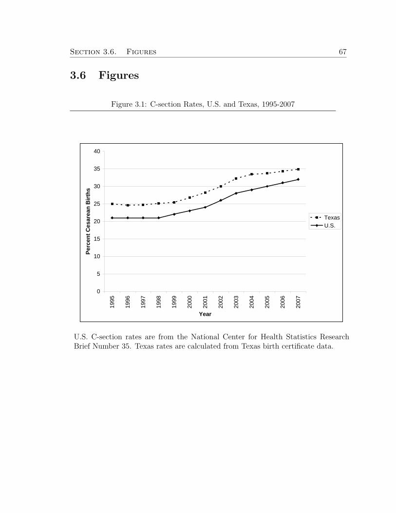
Section 3.6. Figures 67
3.6 Figures
Figure 3.1: C-section Rates, U.S. and Texas, 1995-2007
0
5
10
15
20
25
30
35
40
1995
1996
1997
1998
1999
2000
2001
2002
2003
2004
2005
2006
2007
Year
Perc
ent C
esar
ean
Birt
hs
TexasU.S.
U.S. C-section rates are from the National Center for Health Statistics ResearchBrief Number 35. Texas rates are calculated from Texas birth certificate data.
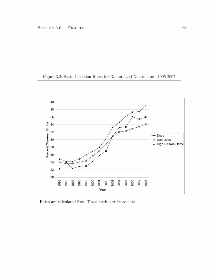
Section 3.6. Figures 68
Figure 3.2: State C-section Rates for Doctors and Non-doctors, 1995-2007
20
22
24
26
28
30
32
34
36
38
40
1995
1996
1997
1998
1999
2000
2001
2002
2003
2004
2005
2006
2007
2008
Year
Perc
ent C
esar
ean
Birt
hs
DocsNon-DocsHigh-Ed Non-Docs
Rates are calculated from Texas birth certificate data.

Section 3.6. Figures 69
Figure 3.3: Gap in C-section Rates for Doctors and Non-doctors Over Time
-0.03
-0.025
-0.02
-0.015
-0.01
-0.005
01996 1999 2002 2005
Year
Perc
enta
ge P
oint
s
Betaci1ci2
beta
Coefficients and confidence intervals are from logistic regressions of C-section indi-cators on doctor indicators. Plot points are from regressions estimated on birthsfrom (i) 1996-1998, (ii) 1999-2001, (iii) 2002-2004, and (iv) 2005-2007.

Section 3.7. Tables 70
3.7 Tables
Table 3.1: Delivery Outcomes for Doctors and Non-doctorsDocs Non-Docs High-ed
No previous C-section Non-DocsC-section 18.8% 19.1% 20.9%Vaginal 81.2% 80.9% 79.1%
Forceps 3.2% 2.6% 3.5%Vacuum 3.4% 4.1% 4.7%Spontaneous 74.6% 74.2% 70.8%
N 23,697 3,722,378 394,374Previous C-sectionC-section 86.0% 87.9% 87.3%Vaginal 14.0% 12.1% 12.7%
Forceps 0.8% 0.6% 0.8%Vacuum 0.9% 0.8% 1.0%Spontaneous 12.2% 10.6% 10.8%
N 3,766 562,749 59,962Table displays self-reported delivery methods for sample ofbirths in Texas from 1995-April 2008. The sample excludesbirths not attended by an MD, not in a hospital, births withmissing maternal age and plural births. The top panel in-cludes only births to mothers who have not previously had aC-section; the bottom panel includes births to mothers whohave had a previous cesarean. Column 1 summarizes deliverymethods when any parent (mother or father) is a doctor, Col-umn 2 for non-doctor parents, and Column 3 for high-educatednon-doctor (masters degree or higher) parents.
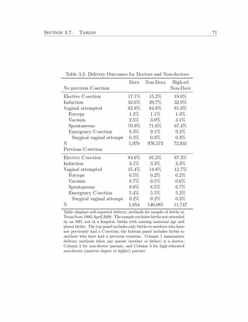
Section 3.7. Tables 71
Table 3.2: Delivery Outcomes for Doctors and Non-doctorsDocs Non-Docs High-ed
No previous C-section Non-DocsElective C-section 17.1% 15.2% 19.0%Induction 32.6% 29.7% 32.8%Vaginal attempted 82.9% 84.8% 81.0%
Forceps 1.3% 1.1% 1.3%Vacuum 2.5% 3.0% 3.1%Spontaneous 70.9% 71.6% 67.4%Emergency C-section 8.3% 9.1% 9.2%
Surgical vaginal attempt 0.3% 0.3% 0.3%N 5,970 976,573 72,931Previous C-sectionElective C-section 84.6% 85.2% 87.3%Induction 3.1% 3.3% 3.3%Vaginal attempted 15.4% 14.8% 12.7%
Forceps 0.5% 0.2% 0.2%Vacuum 0.7% 0.5% 0.6%Spontaneous 8.8% 8.5% 6.7%Emergency C-section 5.4% 5.5% 5.2%
Surgical vaginal attempt 0.2% 0.2% 0.3%N 1,054 146,085 11,747Table displays self-reported delivery methods for sample of births inTexas from 1995-April 2008. The sample excludes births not attendedby an MD, not in a hospital, births with missing maternal age andplural births. The top panel includes only births to mothers who havenot previously had a C-section; the bottom panel includes births tomothers who have had a previous cesarean. Column 1 summarizesdelivery methods when any parent (mother or father) is a doctor,Column 2 for non-doctor parents, and Column 3 for high-educatednon-doctor (masters degree or higher) parents.

Section 3.7. Tables 72
Table 3.3: Summary Statistics, 1995-April 2008Docs Non-docs High-ed Non-docs
Mean Std Dev Mean Std Dev Mean Std Dev
Educational attainment of parents (%) Mean Std. Dev. Mean Std. Dev. Mean Std. Dev.Mother High Education 21.2 40.9 27.0 44.4Father High Education 65.2 47.6 35.0 47.7Both High Education 13.6 34.3Highschool 25.3 43.5College 28.6 45.2High Education 10.6 30.8Mother’s demographicsMother’s age 32.7 4.1 26.3 6.1 31.3 4.5Black (%) 4.7 21.1 11.3 31.7 7.1 25.7Asian (%) 18.9 39.2 3.2 17.7 10.8 31.0Hispanic (%) 12.5 33.1 46.3 49.9 14.8 35.5Married (%) 98.5 12.2 69.1 46.2 96.6 18.2Birth information (%)First birth 43.6 49.6 45.2 49.8 49.7 50.0Previous birth within 18mo 4.5 20.7 6.5 24.7 3.6 18.7Prenatal Care 98.4 12.5 95.8 20.0 98.4 12.4Smoker 0.45 6.70 6.47 24.60 1.36 11.59Early delivery 7.0 25.5 8.6 28.0 6.8 25.2Late delivery 0.042 2.054 0.161 4.006 0.055 2.345Very low birth weight 0.65 8.06 1.10 10.42 0.65 8.06Low birth weight 4.2 20.1 5.4 22.5 3.8 19.0High birth weight 7.1 25.7 7.7 26.7 9.7 29.5Risk factors (%)Diabetes 2.4 15.2 2.9 16.8 2.8 16.6Chronic hypertension 0.54 7.36 0.68 8.24 0.72 8.44Pregnancy-induced hypertension 2.8 16.6 4.2 20.1 3.6 18.7Eclampsia 0.093 3.046 0.261 5.105 0.183 4.278Previous preterm birth 0.43 6.58 0.53 7.28 0.30 5.46Preterm labor 2.3 15.0 2.4 15.4 2.2 14.5Preterm rupture of membranes 1.3 11.3 1.5 12.3 1.2 11.0Complications (%)Meconium 3.6 18.6 4.7 21.2 4.2 20.2Premature rupture of membranes 1.2 10.8 1.5 12.0 1.3 11.3Precipitous labor (≤ 3hours) 1.7 13.0 1.8 13.3 1.5 12.1Prolonged labor (≥ 20hours) 0.50 7.04 0.58 7.60 0.54 7.31Breech / malpresentation 2.4 15.4 2.2 14.8 2.8 16.5Zip code per capita income 29,453 13,046 18,650 8,463 26,172 11,037N 23,697 3,722,378 394,374Table displays means and standard deviations of key explanatory variables for the sample of births in Texasfrom 1995-April 2008. The sample excludes births not attended by an MD, not in a hospital, births withmissing maternal age and plural births. Columns 1 and 2 summarize variables for doctor-parents, Columns3 and 4 for non-doctors, and Columns 5 and 6 for high-education non-doctors.

Section 3.7. Tables 73
Table 3.4: Summary Statistics, 2005-April 2008Docs Non-docs High-ed Non-docs
Mean Std Dev Mean Std Dev Mean Std Dev
Educational attainment of parents (%) Mean Std. Dev. Mean Std. Dev. Mean Std. Dev.Mother High Education 24.6 43.1 33.9 47.4Father High Education 61.0 48.8 25.9 43.8Both High Education 14.4 35.1Highschool 22.0 41.4College 29.3 45.5High Education 7.5 26.3Mother’s demographicsMother’s age 33.0 4.0 26.5 6.1 32.2 4.2Black (%) 5.1 22.1 11.5 31.9 7.1 25.7Asian (%) 22.8 42.0 3.6 18.7 16.5 37.1Hispanic (%) 12.8 33.5 49.8 50.0 14.4 35.1Married (%) 99.0 10.1 75.8 42.8 98.9 10.4Birth information (%)First birth 45.1 49.8 45.0 49.7 51.2 50.0Previous birth within 18mo 4.4 20.5 6.7 25.0 3.3 17.9Prenatal Care 99.1 9.6 95.6 20.5 99.0 9.8Smoker 0.22 4.66 5.48 22.75 0.56 7.47Early delivery 7.8 26.8 9.5 29.4 7.6 26.5Late delivery 0.050 2.241 0.174 4.171 0.058 2.399Very low birth weight 0.67 8.16 1.17 10.74 0.72 8.45Low birth weight 4.9 21.6 5.7 23.2 4.3 20.3High birth weight 5.9 23.6 6.4 24.5 7.5 26.3Risk factors (%)Diabetes 3.3 17.8 4.0 19.6 4.5 20.7Chronic hypertension 0.65 8.06 0.83 9.07 0.85 9.17Pregnancy-induced hypertension 3.5 18.4 4.6 20.9 4.1 19.8Eclampsia 0.017 1.294 0.130 3.602 0.077 2.770Previous preterm birth 0.44 6.59 0.68 8.20 0.31 5.59Preterm labor 1.0 10.1 1.1 10.2 0.7 8.5Preterm rupture of membranes 1.6 12.6 1.8 13.3 1.6 12.5Complications (%)Meconium 3.2 17.5 4.1 19.9 4.2 20.0Premature rupture of membranes 1.6 12.6 1.8 13.3 1.6 12.5Precipitous labor (≤ 3hours) 1.9 13.7 2.2 14.6 1.8 13.3Prolonged labor (≥ 20hours) 0.75 8.65 0.87 9.28 0.73 8.53Breech / malpresentation 0.9 9.6 0.8 8.6 1.0 10.1Zip code per capita income 29,763 12,607 18,914 8,352 27,365 10,950N 5,970 976,573 72,931Table displays means and standard deviations of key explanatory variables for the sample of births in Texasfrom 2005-April 2008. The sample excludes births not attended by an MD, not in a hospital, births withmissing maternal age and plural births. Columns 1 and 2 summarize variables for doctor-parents, Columns3 and 4 for non-doctors, and Columns 5 and 6 for high-education non-doctors.

Section 3.7. Tables 74
Table 3.5: C-section Rates for Doctors and Non-doctors(1) (2) (3) (4) (5)
Any Parent MD -0.0210*** -0.0142*** -0.0132*** -0.0118***(0.00262) (0.00250) (0.00251) (0.00254)
Mother MD -0.0172***(0.00486)
Father MD -0.00998**(0.00319)
Both Parents MD -0.0200**(0.00625)
N 418071 418071 418071 418071 408419Pseudo R-squared 0.00014 0.11 0.17 0.17 0.17Table displays coefficients on doctor dummies from logit regressions of C-section (emergencyor elective) indicators on doctor dummies and various explanatory variables. The specifica-tion in Column 1 contains no additional explanatory variables. The specification in Column2 contains birth information, risk factors, and year and month dummies. The specificationin Column 3 additionally contains complications. The specification in Column (4) splitsthe doctor dummy into three dummies depending on which parents are doctors. It includesbirth information, risk factors, complications and year and month dummies. The specifica-tion in Column 5 is equivalent to that in Column 3 with the addition of zipcode per capitaincome as an explanatory variable. Full table results are in Appendix A. Marginal effectsare presented. Robust standard errors are in parentheses. * indicates significance at the 5%,** at the 1%, and *** at the .1% levels.

Section 3.7. Tables 75
Table 3.6: C-section Rates for Lawyers and NursesLawyers Nurses
(1) (2) (3) (4)Any Parent 0.00366 0.00424
(0.00244) (0.00321)
Mom Only 0.00362 0.00403(0.00443) (0.00340)
Dad Only -0.000578 0.00488(0.00310) (0.0110)
Both Parents 0.0253*** 0.00819(0.00717) (0.0169)
Observations 418071 418071 418071 418071Pseudo R-squared 0.17 0.17 0.17 0.17Table displays coefficients on doctor dummies from logit regressions of C-section(emergency or elective) indicators on lawyer dummies (Columns 1 and 2) andRN dummies (Columns 2 and 3) and explanatory variables (maternal demo-graphics, birth information, risk factors, complications, and year and monthdummies). Columns 1 and 3 include dummies indicating any parent is a lawyeror RN. Columns 2 and 4 include dummies for 3 cases: mother only and fatheronly lawyer/RN and both parents lawyer/RN. Marginal effects are presented.Robust standard errors are in parentheses. * indicates significance at the 5%,** at the 1%, and *** at the .1% levels.

Section 3.7. Tables 76
Table 3.7: Breakdown of Delivery Outcomes for Doctors and Non-doctors
C-section Elective Induction Emergency EmergencyC-section C-section C-section
(1) (2) (3) (4) (5)
Any parent MD -0.0175** -0.0161** 0.00919 -0.00296 -0.00388(0.00610) (0.00498) (0.00652) (0.00377) (0.00370)
Any parent MD X Surgical Vaginal Delivery 0.00869(0.0235)
Surgical vaginal delivery -0.0617***(0.00208)
Observations 78901 78901 78901 64049 64049Pseudo R-squared 0.093 0.069 0.030 0.12 0.13Table displays coefficients on doctor dummies from logit regressions of delivery outcomeindicators on doctor dummies. Sample includes births from 2005-April 2008. In all spec-ifications, explanatory variables include (maternal demographics, birth information, riskfactors, complications, and year and month dummies). The dependent variable for Column1 is any C-section, in Column 2 it is an indicator for elective C-section, in Column 3 in-duction, and in Columns 4 and 5 it is emergency C-section. Marginal effects are presented.Robust standard errors are in parentheses. * indicates significance at the 5%, ** at the 1%,and *** at the .1% levels.

Section 3.7. Tables 77
Table 3.8: Birth Outcomes for Doctors and Non-doctorsDeath Injury NICU
(1) (2) (3) (4) (5) (6)Any Parent MD -13.1 43.8 1.1
(13.2) (67.5) (5.2)Mom Only MD -28.25 55.2 -29.6**
(20.18) (136.3) (9.3)Dad Only MD 6.32 17.8 11.2
(19.05) (80.3) (6.6)Both Parents MD -59.33*** 138.7 12.4
(15.80) (228.8) (14.3)Observations 78901 78901 78901 78901 78901 78901Table displays coefficients on doctor indicators from logit regressions of indicatorsfor birth outcomes on doctor indicators. Sample includes births from 2005-April2008. In all specifications, explanatory variables include (maternal demographics,birth information, risk factors, complications, and year and month dummies). Thedependent variable for Columns 1 and 2 is mortality in hospital, in Columns 3 and 4 itis an indicator for injury to the baby, and in Columns 5 and 6 it is NICU admission.Marginal effects are presented as a percentage of the dependent variable. Robuststandard errors are in parentheses. * indicates significance at the 5%, ** at the 1%,and *** at the .1% levels.

78
Bibliography
[1] Aaronson, D., Barrow, L. and Sander, W. 2007 “Teachers and StudentAchievement in the Chicago Public High Schools.” Journal of Labor Eco-nomics, 25:95-135.
[2] Altonji, J. and Pierret, C. 1999 “Employer Learning and Statistical Dis-crimination.” Quarterly Journal of Economics, 116:313-350.
[3] Arrow, K. 1963 “Uncertainty and the Welfare Economics of Medical Care.”American Economic Review, 5:141-149.
[4] Baicker, K., Buckles, K. and Chandra, A. 2006 “Geographic Variation inthe Appropriate Use of Cesarean Delivery.” Health Affairs, 25.355-367.
[5] Barro, J. and Beaulieu, N. 2003 “Selection and Improvement: PhysicianResponses to Financial Incentives.” National Bureau of Economic ResearchWorking Paper Number 10017.
[6] Bohmer, R., Christensen, C., and Kenagy, J. 2000 “Will disruptive innova-tions cure health care?” Harvard Business Review, 78:102-112.
[7] Bunker, J. and Brown, B. 1974 “The Physician-Patient as an InformedConsumer of Surgical Services.” The New England Journal of Medicine,290:1051-1055.
[8] Burgess, J., Christiansen, C., Michalak, S. and Morris, C. 2000 “MedicalProfiling: Improving Standards and Risk Adjustments Using HierarchicalModels.” Journal of Health Economics, 19:291-309.
[9] Campbell, S., Reeves, D., Kontopantelis, E., Middleton, E., Sibbald, B.and Roland, M. 2007 “Quality of Primary Care in England with the In-troduction of Pay For Performance.” New England Journal of Medicine,357:181-190.
[10] Center for Studying Health System Change. 2007 “Health Tracking Physi-cian Survey.”

BIBLIOGRAPHY 79
[11] Chamberlain, G. 1982 “Multivariate Regression Models For Panel Data.”Journal of Econometrics, 18:5-46.
[12] Chevalier, J. and Ellison, G. 1997 “Career Concerns of Mutual Fund Man-agers.” Quarterly Journal of Economics, 114:389-432.
[13] Chou, Y.J. et Al. 2006 “Do Physicians and their Relatives Have a DecreasedRate of Cesarean Section?” Birth, 33:195-202.
[14] Cromwell, J. and Mitchell, J. 1986 “Physician-Induced Demand forSurgery.” Journal of Health Economics, 5:293-313.
[15] Croxson, B., Propper, C. and Perkins, A. 2001 “Do Doctors Respond toFinancial Incentives? UK Family Doctors and the GP Fundholder Scheme.”Journal of Public Economics, 79:375-398.
[16] Currie, J. and MacLeod, B. “First Do No Harm? Tor Reform and BirthOutcomes.” Quarterly Journal of Economics, 123:795-830.
[17] Cutler, D., Huckman, S. and Landrum, M.B. 2004 “The Role of Informationin Medical Markets: An Analysis of Publicly Reported Outcomes in CardiacSurgery.” American Economic Review, 94(2):342-346.
[18] Cutler, D. and Huckman, R. 2003 “Technology Development and MedicalProductivity: The Diffusion of Angioplasty in New York State.” Journal ofHealth Economics, 22:187-217.
[19] Dranove, D., Satterthwaite, D., Kessler, D., and McClellan, M. 2003 “IsMore Information Better? The Effects of Report Cards on CardiovascularProviders and Consumers.” Journal of Political Economy, 11:555-588.
[20] Epstein, A. 2006 “Do Cardiac Surgery Report Cards Reduce Mortality?Assesing the Evidence.” Medical Care Research Review, 63:403-421.
[21] Epstein, A. and Nicholson, S. 2009 “The Formation and Evolution of Physi-cian Treatment Styles: An Application to Cesearean Sections.” Journal ofHealth Economics, 28:1126-1140.
[22] Fama, E. 1980 “Agency Problems and the Theory of the Firm.” Journal ofPolitical Economy, 88:288-307.
[23] Farber, H. and Gibbons, R. 1996 “Learning and Wage Dynamics.” QuarterlyJournal of Economics, 111:1007-47.
[24] Feldstein, M. 1970 “The Rising Price of Physician Services.” The Review ofEconomics and Statistics, 52: 121-133.

BIBLIOGRAPHY 80
[25] Fong, K. 2009 “Evaluating Skilled Experts: Optimal Scoring Rules for Sur-geons.” mimeo, Stanford University.
[26] Fournier, G. and McInnes, M. 2002 “The Effects of Managed Care on Med-ical Referrals and the Quality of Specialty Care.” Journal of Industrial Eco-nomics, 50:457-73.
[27] Fuchs, V. 1978 “The Supply of Surgeons and the Demand for Operations.”Journal of Human Resources, 13 (Supplement):35-36.
[28] Gaynor, M. and Pauly, M. 1990 “Compensation and Productive Efficiencyin Partnerships: Evidence from Medical Group Practice.” Journal of Polit-ical Economy, 93:3.
[29] Gaynor, M., Rebitzer, J., and Taylor, L. 2004 “Incentives in Health Main-tenance Organizations.” Journal of Political Economy, 112:915-931.
[30] Gibbons, R. 1997 “Incentives and Careers in Organizations.” Chapter 1 inVolume II of D. Kreps and K. Wallis (eds.), Advances in Economics andEconometrics: Theory and Applications, Cambridge University Press.
[31] Gibbons, R. and Katz, L. 1991 “Layoffs and Lemons.” Journal of LaborEconomics, 9:351-380.
[32] Gibbons, R. and Murphy, K. 1992 “Optimal Incentive Contracts in thePresence of Career Concerns: Theory and Evidence.” Journal of PoliticalEconomy, 100:468-505.
[33] Girion, L. “More C-sections, More Problems” Los Angeles Times. 17 May2009.
[34] Glance, L., Dick, A., Mukamel, D., Li, Y. and Osler, T. 2008 “Are HighQuality Cardiac Surgeons Less Likely to Operate on High-Risk PatientsCompared to Low Quality Surgeons? Evidence from New York State.”Health Services Research, 43:300-312.
[35] Glance, L., Dick, A., Osler, T., Li, Y. and Mukamel, D. 2006 “Impact ofChanging the Statistical Methodology on Hospital and Surgeon Ranking:The Case of the New York State Cardiac Surgery Report Card.” MedicalCare, 44:311-9.
[36] Glazer, J., McGuire, T. and Newhouse, J. 2007 “Using Performance Mea-sures to Motivate Report-averse and Report-loving Agents.” Journal ofHealth Economics, 26:1170-1189.

BIBLIOGRAPHY 81
[37] Green, J. and Wintfeld, N. 1995 “Report Cards on Cardiac Surgeons -Assessing New York State’s Approach.” New England Journal of Medicine,332:1229-32.
[38] Greenwald, B. 1986 “Adverse Selection in the Labor Market.” Review ofEconomic Studies, 53:325-347.
[39] Gruber, J. and Owings, M. 1996 “Physician Financial Incentives and Ce-sarean Section Delivery.” RAND Journal of Economics, 4.
[40] Gruber, J., Kim, J., and Mayzlin, D. 1999 “Physician Fees and ProcedureIntensity: The Case of Cesarean Delivery.” Journal of Health Economics,18:473-490.
[41] Hemenway, D., Killen, A., Cashman, S., Parks, C. and Bicknell, W.1990 “Physician Response to Financial Incentives: Evidence from a For-profit Ambulatory Care Center.” The New England Journal of Medicine,322:1059-63.
[42] Hannan, E., Kilburn, H., O’Donnell, J., Lukacik, G., and Shields, E. 1990“An Analysis of Risk Factors and Hospital Mortality Rates.” Journal of theAmerican Medical Association, 264:2768-74.
[43] Hannan, E., Kumar, M., Racz, A, Siu, A., and Chassin, M. 1994 “New YorkState’s Cardiac Surgery Reporting System: Four Years Later.” Annals ofThoracic Surgery, 6:1852-57.
[44] Hanushek, E. 1971 “Teacher Characteristics and Gains in Student Achieve-ment: Estimation Using Micro Data.” American Economic Review, 60:280-288.
[45] Harris, M. and Holmstrom, B. 1982 “A Theory of Wage Dynamics.” TheReview of Economic Studies, 49:315-333.
[46] Hartz, A., Kuhn, E. and Pulido, J. 1999 “Prestige of Training Programs andExperience of Bypass Surgeons as Factors in Adjusted Patient MortalityRates.” Medical Care, 37:99-103.
[47] Holmstrom, B. 1979 “Managerial Incentive Problems: A Dynamic Perspec-tive.” In Essays in Economics and Management in Honor of Lars Wahlbeck.Helsinki: Swedish School of Economics. Republished in Review of EconomicStudies, 66 (1999):169-82.

BIBLIOGRAPHY 82
[48] Jacob, B. and Lefgren, L. 2008 “Principals as Agents: Subjective Perfor-mance Measurement in Education.” Journal of Labor Economics, 26:101-136.
[49] Jovanovic, B. 1979 “Job Matching and the Theory of Turnover.” Journal ofPolitical Economy, 87:972-990.
[50] Kane, T., Rockoff, J. and Staiger, D. 2006 “What Does Certification TellUs About Teacher Effectiveness? Evidence from New York City.” NationalBureau of Economic Research Working Paper Number 12155.
[51] Kane, T. and Staiger, D. 2002 “The Promise and Pitfalls of Using ImpreciseSchool Accountability Measures.” Journal of Economic Perspectives, 16:91-114.
[52] Landon, Hauth, Leveno, Spong, Leindecker, Varner et al 2004 “Maternaland Perinatal Outcomes Associated with a Trial of Labor After Prior Ce-sarean Delivery.” New England Journal of Medicine, 351:2581-2589.
[53] Lazear, E. and Rosen, S. 1981 “Rank-Order Tournaments as OptimumLabor Contracts.” Journal of Political Economy, 89:841-864.
[54] Levitt, S. and Syverson, C. “Market Distortions When Agents are BetterInformed: The Value of Information in Real Estate Transactions.” TheReview of Economics and Statistics, 90: 599-611.
[55] Localio, A., Hamory, B., Fisher, A., and TenHave, T. 1997 “The PublicRelease of Hospital and Physician Mortality Data in Pennsylvania: A CaseStudy.” Medical Care, 35:272-286.
[56] LeGrand, J. 1999 “Competition, Co-operation or Control? Tales from theBritish National Health Service.” Health Affairs, 18:27-39.
[57] Lyndon-Rochelle, M., Holt, V., Martin, D. and Easterling, T. 2000 “As-sociation Between Method of Delivery and Maternal Rehospitalization.”Journal of the American Medical Association, 283:2411-2416.
[58] Lyndon-Rochelle, M., Holt, V., Easterling, T. and Martin,D. 2001 “Riskof Uterine Rupture During Labor Among Women with a Prior CesareanDelivery.” New England Journal of Medicine, 345:3-8.
[59] McClellan, M. and Staiger, D. 1999 “The Quality of Health Care Providers.”National Bureau of Economic Research Working Paper Number 7327.

BIBLIOGRAPHY 83
[60] McGuire, T. and Pauly, M. 1991 “Physician Response to Fee Changes withMultiple Players.” Journal of Health Economics, 10:385-410.
[61] Morris, C. 1983 “Parametric Empirical Bayes Inference: Theory and Ap-plications.” Journal of the American Statistical Association, 78:47-65.
[62] Mullen, K., Frank, R. and Rosenthal, M. 2009 “Can You Get What YouPay For? Pay-For-Performance and the Quality of Healthcare Providers.”National Bureau of Economic Research Working Paper Number 14886.
[63] Mundlak, Y. 1978 “On the Pooling of Time Series and Cross Section Data.”Econometrica, 46:69-85.
[64] Newhouse, J. 1970 “A Model of Physician Pricing.” Southern EconomicJournal, 37:174-183.
[65] Newhouse, J. 1992 “Medical Care Costs: How Much Welfare Loss?” Jour-nal of Economic Perspectives, 6:3-21.
[66] Neyman, J. Scott, E. 1948 “Consistent Estimates based on Partially Con-sistent Observations.” Econometrica, 16:1-32.
[67] Normand, S., Glickman, M. and Gatsonis, C. 1997 “Statistical Methods forProfiling Providers of Medical Care: Issues and Applications.” Journal ofthe American Statistical Association, 92:803-814.
[68] O’Connor, G., Plume, S., Olmstead, E., et al. 1991 “A Regional ProspectiveStudy of In-hospital Mortality Associated with Coronary Artery BypassGrafting.” Journal of the American Medical Association, 266:803-9.
[69] Pendergast, C. 1998 “The Provision of Incentives in Firms.” Journal ofEconomic Literature, 37:7-63.
[70] Peterson, E., DeLong, J., Jollis, J., Muhlbaier, L. and Mark, D. 1998 “TheEffects of New York’s Bypass Surgery Provider Profiling on Access to Careand Patient Outcomes in the Elderly.” Journal of the American College ofCardiology, 32:993-99.
[71] Reinhardt, U. 1985 “The Theory of Physician-Induced Demand: ReflectionsAfter a Decade.” Journal of Health Economics, 4:187-193.
[72] Rockoff, J. 2004 “The Impact of Individual Teachers on Student Achieve-ment: Evidence from Panel Data.” American Economic Review, 94:247-252.
[73] Rosenthal, M. and Frank, R. 2006 “What Is the Empirical Basis for Payingfor Quality in Health Care?” Medical Care Research and Review, 63:135-57.

BIBLIOGRAPHY 84
[74] Rosenthal, M., Frank, R., Li, Z. and Epstein, A. 2005 “Early Experi-ence with Pay-for-Performance: From Concept to Practice.” Journal of theAmerican Medical Association, 294:1788-93.
[75] Schneider, E. and Epstein, A. 1996 “Influence of Cardiac-Surgery Perfor-mance Reports on Referral Practices and Access to Care: A Survey ofCardiovascular Specialists.” New England Journal of Medicine, 335:251-56.
[76] Shea, D., Stuart, B., Vasey, J. and Nag, S. 1999 “Medicare Physician Re-ferral Patterns.” Health Services Research, 34(1):331-345.
[77] TenHave, T. and Localio, R. 1999 “Empirical Bayes Estimation of RandomEffects Parameters in Mixed Effects Logistic Regression Models.” Biomet-rics, 55:1022-1029.
[78] Thomas, N., Longford, N. and Rolph, J. 1994 “Empirical Bayes Methodsfor Estimating Hospital-Specific Mortality Rates.” Statistics in Medicine,13:889-903.
[79] U.S. Department of Health and Human Services. Healthy People 2010. 2nded. With Understanding and Improving Health and Objectives for Im-proving Health. 2 vols. Washington, DC: U.S. Government Printing Office,November 2000.
[80] Wennberg, J., Fisher, E., Goodman, D. and Skinner, J. 2008 “Trackingthe Care of Patients with Severe Chronic Illness.” The Dartmouth Atlas ofHealth Care.
[81] Wilensky, G. and Rossiter, L. 1983 “The Relative Importance of Physician-Induced Demand in the Demand for Medical Care.” Milbank Quarterly,61:252-299.
[82] Williams, S., Nash, D. and Goldfarb, N. 1991 “Differences in Mortalityfrom Coronary Artery Bypass Graft Surgery at Five Teaching Hospitals.”Journal of the American Medical Association, 266:174-183.

85
Appendix A
Appendix to Chapter 3
Supplementary Tables
Table A.1: C-Section Rates for Doctors and High-Educated Non-doctors, FullCoefficient List
(1) (2) (3) (4) (5)Any Parent / -0.021 -0.014 -0.013 -0.017 -0.012
Mom Only (0.0026) (0.0025) (0.0025) (0.0049) (0.0025)Dad Only -0.010
(0.0032)Both Parents MD -0.020
(0.0063)Educational attainment of parentsMother High Ed 0.012 0.011 0.011 0.0094
(0.0015) (0.0016) (0.0016) (0.0016)Both High Ed -0.0053 -0.0057 -0.0054 -0.0054
(0.0014) (0.0014) (0.0014) (0.0014)Mother’s demographicsMother’s age 0.0020 0.00032 0.00031 0.0011
(0.0014) (0.0014) (0.0014) (0.0014)Mother’s age 0.00011 0.00013 0.00013 0.00012
squared (0.000021) (0.000021) (0.000021) (0.000021)Black 0.063 0.072 0.072 0.067
(0.0028) (0.0029) (0.0029) (0.0029)Asian 0.002128 0.0080 0.0080 0.0086
(0.0019) (0.0020) (0.0020) (0.0020)Hispanic 0.045 0.050 0.050 0.046
(0.0019) (0.0019) (0.0019) (0.0020)Married -0.010 -0.013 -0.013 -0.012
(0.0034) (0.0035) (0.0035) (0.0035)Birth informationFirst birth 0.22 0.22 0.22 0.22
(0.0013) (0.0014) (0.0014) (0.0014)Birth w/in -0.017 -0.017 -0.017 -0.017
18 months (0.0039) (0.0040) (0.0040) (0.0041)Prenatal Care -0.00064 -0.0018 -0.0018 -0.0018
(0.0049) (0.0050) (0.0050) (0.0050)Smoker 0.041 0.041 0.041 0.040
(0.0061) (0.0062) (0.0062) (0.0063)Early delivery 0.063 0.055 0.055 0.054

86
Table A.1: (continued)
(1) (2) (3) (4) (5)(0.0033) (0.0033) (0.0033) (0.0033)
Late delivery 0.040 0.037 0.037 0.039(0.027) (0.028) (0.028) (0.029)
Very LBW 0.23 0.22 0.22 0.21(0.012) (0.012) (0.012) (0.013)
LBW 0.068 0.065 0.065 0.066(0.0040) (0.0040) (0.0040) (0.0041)
HBW 0.11 0.11 0.11 0.11(0.0025) (0.0025) (0.0025) (0.0026)
Risk factorsDiabetes 0.056 0.051 0.051 0.049
(0.0039) (0.0040) (0.0040) (0.0040)Chronic hypertension 0.082 0.081 0.081 0.079
(0.0080) (0.0082) (0.0082) (0.0083)Preg.-ind. hypertension 0.091 0.092 0.092 0.090
(0.0036) (0.0037) (0.0037) (0.0037)Eclampsia 0.17 0.19 0.19 0.18
(0.018) (0.019) (0.019) (0.019)Prev. preterm -0.011 -0.020 -0.020 -0.017
birth (0.013) (0.013) (0.013) (0.013)Preterm labor -0.0085 -0.023 -0.023 -0.023
(0.0042) (0.00412) (0.00412) (0.00415)Preterm membrane -0.038 -0.055 -0.055 -0.055
rupture (0.0045) (0.0045) (0.0045) (0.0046)ComplicationsMeconium 0.020 0.020 0.020
(0.0030) (0.0030) (0.0030)Prem. membrane 0.023 0.023 0.021
rupture (0.0061) (0.0061) (0.0061)Labor ≤ 3hrs. -0.15 -0.15 -0.15
(0.0023) (0.0023) (0.0022)Labor ≥ 20hrs. 0.13 0.13 0.13
(0.010) (0.010) (0.010)Breech 0.76 0.76 0.76
(0.0029) (0.0029) (0.0030)
Per capita -7.3e-07income (d) (5.78e-08)
N 418,071 418,071 418,071 418,071 408,419Pseudo R-squared 0.00014 0.11 0.17 0.17 0.17Table displays coefficients from logit regressions of indicators for C-section on doctorindicators and explanatory variables. Sample includes births from 1995-April 2008.All specifications include year and month dummies. Marginal effects are presented.Robust standard errors are in parentheses. * indicates significance at the 5%, ** atthe 1%, and *** at the .1% levels.