Embed Size (px)
Citation preview

Submitted to the Annals of StatisticsarXiv: arXiv:0000.0000
RATE-OPTIMAL GRAPHON ESTIMATION
By Chao Gao, Yu Lu and Harrison H. Zhou
Yale University
Network analysis is becoming one of the most active researchareas in statistics. Significant advances have been made recently ondeveloping theories, methodologies and algorithms for analyzing net-works. However, there has been little fundamental study on optimalestimation. In this paper, we establish optimal rate of convergencefor graphon estimation. For the stochastic block model with k clus-ters, we show that the optimal rate under the mean squared error isn−1 log k + k2/n2. The minimax upper bound improves the existingresults in literature through a technique of solving a quadratic equa-tion. When k ≤
√n logn, as the number of the cluster k grows, the
minimax rate grows slowly with only a logarithmic order n−1 log k. Akey step to establish the lower bound is to construct a novel subset ofthe parameter space and then apply Fano’s lemma, from which we seea clear distinction of the nonparametric graphon estimation problemfrom classical nonparametric regression, due to the lack of identifia-bility of the order of nodes in exchangeable random graph models.As an immediate application, we consider nonparametric graphon es-timation in a Holder class with smoothness α. When the smoothnessα ≥ 1, the optimal rate of convergence is n−1 logn, independent of
α, while for α ∈ (0, 1), the rate is n−2α
α+1 , which is, to our surprise,identical to the classical nonparametric rate.
1. Introduction. Network analysis [17] has gained cosiderable researchinterests in both theories [7] and applications [43, 16]. A lot of recent workhas been focusing on studying networks from a nonparametric perspective[7], following the deep advancement in exchangeable arrays [3, 25, 27, 13].In this paper, we study the fundamental limits in estimating the underlyinggenerating mechanism of network models, called graphon. Though variousalgorithms have been proposed and analyzed [10, 38, 44, 2, 9], it is not clearwhether the convergence rates obtained in these works can be improved, andnot clear what the differences and connections are between nonparametricgraphon estimation and classical nonparametric regression. The results ob-tained in this paper provide answers to those questions. We found manyexisting results in literature are not sharp. Nonparametric graphon estima-
MSC 2010 subject classifications: Primary 60G05Keywords and phrases: network, graphon, stochastic block model, nonparametric re-
gression, minimax rate
1
2 GAO, LU AND ZHOU
tion can be seen as nonparametric regression without knowing design. Whenthe smoothness of the graphon is small, the minimax rate of graphon esti-mation is identical to that of nonparametric regression. This is surprising,since graphon estimation seems to be a more difficult problem, for whichthe design is not observed. When the smoothness is high, we show that theminimax rate does not depend on the smoothness anymore, which providesa clear distinction between nonparametric graphon estimation and nonpara-metric regression.
We consider an undirected graph of n nodes. The connectivity can beencoded by an adjacency matrix Aij taking values in 0, 1n×n. The valueof Aij stands for the presence or the absence of an edge between the i-thand the j-th nodes. The model in this paper is Aij = Aji ∼ Bernoulli(θij)for 1 ≤ j < i ≤ n, where
(1.1) θij = f(ξi, ξj), i 6= j ∈ [n].
The sequence ξi are random variables sampled from a distribution Pξsupported on [0, 1]n. A common choice for the probability Pξ is i.i.d. uniformdistribution on [0, 1]. In this paper, we allow Pξ to be any distribution, sothat the model (1.1) is studied to its full generality. Given ξi, we assumeAij are independent for 1 ≤ j < i ≤ n, and adopt the convention thatAii = 0 for each i ∈ [n]. The nonparametric model (1.1) is inspired bythe advancement of graph limit theory [32, 13, 31]. The function f(x, y),which is assumed to be symmetric, is called graphon. This concept plays asignificant role in network analysis. Since graphon is an object independentof the network size n, it gives a natural criterion to compare networks ofdifferent sizes. Moreover, model based prediction and testing can be donethrough graphon [30]. Besides nonparametric models, various parametricmodels have been proposed on the matrix θij to capture different aspectsof the network [23, 24, 37, 36, 19, 22, 1, 28].
The model (1.1) has a close relation to the classical nonparametric regres-sion problem. We may view the setting (1.1) as modeling the mean of Aij bya regression function f(ξi, ξj) with design (ξi, ξj). In a regression problem,the design points (ξi, ξj) are observed, and the function f is estimatedfrom the pair (ξi, ξj), Aij. In contrast, in the graphon estimation setting,(ξi, ξj) are latent random variables, and f can only be estimated fromthe response Aij. This causes an identifiability problem, because withoutobserving the design, there is no way to associate the value of f(x, y) with(x, y). In this paper, we consider the following loss function
1
n2
∑i,j∈[n]
(θij − θij)2
RATE-OPTIMAL GRAPHON ESTIMATION 3
to overcome the identifiability issue. This is identical to the loss functionwidely used in the classical nonparametric regression problem with the form
1
n2
∑i,j∈[n]
(f(ξi, ξj)− f(ξi, ξj)
)2.
Even without observing the design (ξi, ξj), it is still possible to estimatethe matrix θij by exploiting its underlying structure modeled by (1.1).
We first consider θij of a block structure. This stochastic block model,proposed by [24], is serving as a standard data generating process in networkcommunity detection problem [7, 40, 4, 26, 29, 8]. We denote the parameterspace for θij by Θk, where k is the number of clusters in the stochasticblock model. In total, there are an order of k2 number of blocks in θij. Thevalue of θij only depends on the clusters that the i-th and the j-th nodesbelong to. The exact definition of Θk is given in Section 2.2. For this setting,the minimax rate for estimating the matrix θij is as follows.
Theorem 1.1. Under the stochastic block model, we have
infθ
supθ∈Θk
E
1
n2
∑i,j∈[n]
(θij − θij)2
k2
n2+
log k
n,
for any 1 ≤ k ≤ n.
The convergence rate has two terms. The first term k2/n2 is due to thefact that we need to estimate an order of k2 number of unknown parameterswith an order of n2 number of observations. The second term n−1 log k,which we coin as the clustering rate, is the error induced by the lack ofidentifiability of the order of nodes in exchangeable random graph models.Namely, it is resulted from the unknown clustering structure of the n nodes.This term grows logarithmically as the number of clusters k increases, whichis different from what is obtained in literature [10] based on lower rankmatrix estimation.
We also study the minimax rate of estimating θij modeled by the re-lation (1.1) with f belonging to a Holder class Fα(M) with smoothness α.The class Fα(M) is rigorously defined in Section 2.3. The result is stated inthe following theorem.
Theorem 1.2. Consider the Holder class Fα(M), defined in Section 2.3.We have
infθ
supf∈Fα(M)
supξ∼Pξ
E
1
n2
∑i,j∈[n]
(θij − θij)2
n−
2αα+1 , 0 < α < 1,
lognn , α ≥ 1,
4 GAO, LU AND ZHOU
where the expectation is jointly over Aij and ξi.
The approximation of piecewise block function to an α-smooth graphonf yields an additional error at the order of k−2α (see Lemma 2.1). In viewof the minimax rate in Theorem 1.1, picking the best k to trade off thesum of the three terms k−2α, k2/n2, and n−1 log k gives the minimax ratein Theorem 1.2.
The minimax rate reveals a new phenomenon in nonparametric estima-tion. When the smoothness parameter α is smaller than 1, the optimal rateof convergence is the typical nonparametric rate. Note that the typical non-
parametric rate is N−2α
2α+d [41], where N is the number of observations andd is the function dimension. Here, we are in a two-dimensional setting withnumber of observations N n2 and dimension d = 2. Then the correspond-
ing rate is N−2α
2α+d n−2αα+1 . Surprisingly, in Theorem 1.2 for the regime
α ∈ (0, 1), we get the exact same nonparametric minimax rate, though weare not given the knowledge of the design (ξi, ξj). The cost of not ob-serving the design is reflected in the case with α ≥ 1. In this regime, thesmoothness of the function does not help improve the rate anymore. Theminimax rate is dominated by n−1 log n, which is essentially contributed bythe logarithmic cardinality of the set of all possible assignments of n nodesto k clusters. A distinguished feature of Theorem 1.2 to note is that we donot impose any assumption on the distribution Pξ.
To prove Theorem 1.1 and Theorem 1.2, we develop a novel lower boundargument (see Section 3.3 and Section 4.2), which allows us to correctlyobtain the packing number of all possible assignments. The packing numbercharacterizes the difficulty brought by the ignorance of the design (ξi, ξj) inthe graphon model or the ignorance of clustering structure in the stochasticblock model. Such argument may be of independent interest, and we expectits future applications in deriving minimax rates of other network estimationproblems.
Our work on optimal graphon estimation is closely connected to a grow-ing literature on nonparametric network analysis. For estimating the ma-trix θij of stochastic block model, [10] viewed θij as a rank-k matrixand applied singular value thresholding on the adjacency matrix. The con-vergence rate obtained is
√k/n, which is not optimal compared with the
rate n−1 log k + k2/n2 in Theorem 1.1. For nonparametric graphon esti-mation, [44] considered estimating f in a Holder class with smoothness
α and obtained the rate√n−α/2log n under a closely related loss func-
tion. The work by [9] obtained the rate n−1 log n for estimating a Lips-chitz f , but they imposed strong assumptions on f . Namely, they assumed

RATE-OPTIMAL GRAPHON ESTIMATION 5
L2|x − y| ≤ |g(x) − g(y)| ≤ L1|x − y| for some constants L1, L2, withg(x) =
∫ 10 f(x, y)dy. Note that this condition excludes the stochastic block
model, for which g(x) − g(y) = 0 when different x and y are in the samecluster. Local asymptotic normality for stochastic block model was estab-lished in [6]. A method of moment via tensor decomposition was proposedby [5], but it is without explicit convergence rate stated.
Organization. The paper is organized as follows. In Section 2, we statethe main results of the paper, including both upper and lower bounds forstochastic block model and nonparametric graphon estimation. Section 3 is adiscussion section, where we discuss possible generalization of the model, re-lation to nonparametric regression without knowing design and lower boundtechniques used in network analysis. The main body of the technical proofsare presented in Section 4, and the remaining proofs are stated in the sup-plementary material.
Notation. For any positive integer d, we use [d] to denote the set 1, 2, ..., d.For any a, b ∈ R, let a ∨ b = max(a, b) and a ∧ b = min(a, b). The floorfunction bac is the largest integer no greater than a, and the ceiling functiondae is the smallest integer no less than a. For any two positive sequencesan and bn, an bn means there exists a constant C > 0 independentof n, such that C−1bn ≤ an ≤ Cbn for all n. For any aij, bij ∈ Rn×n,
we denote the `2 norm by ||a|| =√∑
i,j∈[n] a2ij and the inner product by
〈a, b〉 =∑
i,j∈[n] aijbij . Given any set S, |S| denotes its cardinality, andIx ∈ S stands for the indicator function which takes value 1 when x ∈ Sand takes value 0 when x /∈ S. For a metric space (T, ρ), the covering numberN (ε, T, ρ) is the smallest number of balls with radius ε and centers in T tocover T , and the packing numberM(ε, T, ρ) is the largest number of pointsin T that are at least ε away from each other. The symbols P and E standfor generic probability and expectation, whenever the distribution is clearfrom the context.
2. Main Results. In this section, we present the main results of thepaper. We first introduce the estimation procedure in Section 2.1. The min-imax rates of stochastic block and nonparametric graphon estimation arestated in Section 2.2 and Section 2.3, respectively.
2.1. Methodology. We are going to propose an estimator for both stochas-tic block model and nonparametric graphon estimation under Holder smooth-ness. To introduce the estimator, let us define the set Zn,k = z : [n]→ [k]
6 GAO, LU AND ZHOU
to be the collection of all possible mappings from [n] to [k] with some inte-gers n and k. Given a z ∈ Zn,k, the sets z−1(a) : a ∈ [k] form a partitionof [n], in the sense that ∪a∈[k]z
−1(a) = [n] and z−1(a) ∩ z−1(b) = ∅ for anya 6= b ∈ [k]. In other words, z defines a clustering structure on the n nodes. Itis easy to see that the cardinality of Zn,k is kn. Given a matrix ηij ∈ Rn×n,and a partition function z ∈ Zn,k, we use the following notation to denotethe block average on the set z−1(a)× z−1(b). That is,
(2.1) ηab(z) =1
|z−1(a)||z−1(b)|∑
i∈z−1(a)
∑j∈z−1(b)
ηij , for a 6= b ∈ [k],
and when |z−1(a)| > 1,
(2.2) ηaa(z) =1
|z−1(a)|(|z−1(a)| − 1)
∑i 6=j∈z−1(a)
ηij , for a ∈ [k].
For any Q = Qab ∈ Rk×k and z ∈ Zn,k, define the objective function
L(Q, z) =∑a,b∈[k]
∑(i,j)∈z−1(a)×z−1(b)
i 6=j
(Aij −Qab)2.
For any optimizer of the objective function,
(2.3) (Q, z) ∈ argminQ∈Rk×k,z∈Zn,k
L(Q, z),
the estimator of θij is defined as
(2.4) θij = Qz(i)z(j), i > j,
and θij = θji for i < j. Set the diagonal element by θii = 0. The proce-dure (2.4) can be understood as first clustering the data by an estimated zand then estimating the model parameters via block averages. By the leastsquares formulation, it is easy to observe the following property.
Proposition 2.1. For any minimizer (Q, z), the entries of Q has rep-resentation
(2.5) Qab = Aab(z),
for all a, b ∈ [k].
RATE-OPTIMAL GRAPHON ESTIMATION 7
The representation of the solution (2.5) shows that the estimator (2.4)is essentially doing a histogram approximation after finding the optimalcluster assignment z ∈ Zn,k according to the least squares criterion (2.3).In the classical nonparametric regression problem, it is known that a simplehistogram estimator cannot achieve optimal convergence rate for α > 1[41]. However, we are going to show that this simple histogram estimatorachieves optimal rates of convergence under both stochastic block model andnonparametric graphon estimation settings.
Similar estimators using the Bernoulli likelihood function have been pro-posed and analyzed in the literature [7, 46, 44, 38]. Instead of using the like-lihood function of Bernoulli distribution, the least squares estimator (2.3)can be viewed as maximizing Gaussian likelihood. This allows us to obtainoptimal convergence rates with cleaner analysis.
2.2. Stochastic Block Model. In the stochastic block model setting, eachnode i ∈ [n] is associated with a label a ∈ [k], indicating its cluster. Theedge Aij is a Bernoulli random variable with mean θij . The value of θij onlydepends on the clusters of the i-th and the j-th nodes. We assume θij isfrom the following parameter space,
Θk =
θij ∈ [0, 1]n×n : θii = 0, θij = Qab = Qba
for (i, j) ∈ z−1(a)× z−1(b) for some Qab ∈ [0, 1] and z ∈ Zn,k
.
Namely, the partition function z assigns cluster to each node, and the valueof Qab measures the intensity of link between the a-th and the b-th clusters.The least squares estimator (2.3) attains the following convergence rate forestimating θij.
Theorem 2.1. For any constant C ′ > 0, there is a constant C > 0 onlydepending on C ′, such that
1
n2
∑i,j∈[n]
(θij − θij)2 ≤ C(k2
n2+
log k
n
),
with probability at least 1 − exp(−C ′n log k), uniformly over θ ∈ Θk. Fur-thermore, we have
supθ∈Θk
E
1
n2
∑i,j∈[n]
(θij − θij)2
≤ C1
(k2
n2+
log k
n
),
8 GAO, LU AND ZHOU
for all k ∈ [n] with some universal constant C1 > 0.
Theorem 2.1 characterizes different convergence rates for k in differentregimes. Suppose k nδ for some δ ∈ [0, 1]. Then the convergence rate inTheorem 2.1 is
(2.6)k2
n2+
log k
n
n−2 k = 1,
n−1 δ = 0, k ≥ 2,
n−1 log n δ ∈ (0, 1/2],
n−2(1−δ) δ ∈ (1/2, 1].
The result completely characterizes the convergence rates for stochasticblock model with any possible number of clusters k. Depending on whetherk is small, moderate, or large, the convergence rates behave differently.
The convergence rate, in terms of k, has two parts. The first part k2/n2 iscalled the nonparametric rate. It is determined by the number of parametersand the number of observations of the model. For the stochastic block modelwith k clusters, the number of parameters is k(k+1)/2 k2 and the numberof observations is n(n + 1)/2 n2. The second part n−1 log k is called theclustering rate. Its presence is due to the unknown labels of the n nodes. Ourresult shows the clustering rate is logarithmically depending on the numberof clusters k. From (2.6), we observe that when k is small, the clusteringrate dominates. When k is large, the nonparametric rate dominates.
To show that the rate in Theorem 2.1 cannot be improved, we obtain thefollowing minimax lower bound.
Theorem 2.2. There exists a universal constant C > 0, such that
infθ
supθ∈Θk
P
1
n2
∑i,j∈[n]
(θij − θij)2 ≥ C(k2
n2+
log k
n
) ≥ 0.8,
and
infθ
supθ∈Θk
E
1
n2
∑i,j∈[n]
(θij − θij)2
≥ C(k2
n2+
log k
n
),
for any k ∈ [n].
The upper bound of Theorem 2.1 and the lower bound of Theorem 2.2immediately imply the minimax rate in Theorem 1.1.
RATE-OPTIMAL GRAPHON ESTIMATION 9
2.3. Nonparametric Graphon Estimation. Let us proceed to nonpara-metric graphon estimation. For any i 6= j, Aij is sampled from the followingprocess,
(ξ1, ..., ξn) ∼ Pξ, Aij |(ξi, ξj) ∼ Bernoulli(θij), where θij = f(ξi, ξj).
For i ∈ [n], Aii = θii = 0. Conditioning on (ξ1, ..., ξn), Aij is independentacross i, j ∈ [n]. To completely specify the model, we need to define thefunction class of f on [0, 1]2. Since f is symmetric, we only need to specifyits value on D = (x, y) ∈ [0, 1]2 : x ≥ y. Define the derivative operator by
∇jkf(x, y) =∂j+k
(∂x)j(∂y)kf(x, y),
and we adopt the convention ∇00f(x, y) = f(x, y). The Holder norm isdefined as
||f ||Hα = maxj+k≤bαc
supx,y∈D
|∇jkf(x, y)|+ maxj+k=bαc
sup(x,y)6=(x′,y′)∈D
|∇jkf(x, y)−∇jkf(x′, y′)|(|x− x′|+ |y − y′|)α−bαc
.
The Holder class is defined by
Hα(M) = |f ||Hα ≤M : f(x, y) = f(y, x) for x ≥ y ,
where α > 0 is the smoothness parameter and M > 0 is the size of the class,which is assumed to be a constant. When α ∈ (0, 1], a function f ∈ Hα(M)satisfies the Lipschitz condition
(2.7) |f(x, y)− f(x′, y′)| ≤M(|x− x′|+ |y − y′|)α,
for any (x, y), (x′, y′) ∈ D. In the network model, the graphon f is assumedto live in the following class,
Fα(M) = 0 ≤ f ≤ 1 : f ∈ Hα(M) .
We have mentioned that the convergence rate of graphon estimation is es-sentially due to the stochastic block model approximation of f in a Holderclass. This intuition is established by the following lemma, whose proof isgiven in the supplementary material.
Lemma 2.1. There exists z∗ ∈ Zn,k, sastisfying,
1
n2
∑a,b∈[k]
∑i 6=j:z∗(i)=a,z∗(j)=b
(θij − θab(z∗)
)2≤ CM2
(1
k2
)α∧1
,
for some universal constant C > 0.
10 GAO, LU AND ZHOU
The graph limit theory [32] suggests Pξ to be an i.i.d. uniform distributionon the interval [0, 1]. For the estimating procedure (2.3) to work, we allow Pξto be any distribution. The upper bound is attained over all distributionsPξ uniformly. Combining Lemma 2.1 and Theorem 2.1 in an appropriatemanner, we obtain the convergence rate for graphon estimation by the leastsquares estimator (2.3).
Theorem 2.3. Choose k = dn1
α∧1+1 e. Then for any C ′ > 0, there existsa constant C > 0 only depending on C ′ and M , such that
1
n2
∑i,j∈[n]
(θij − θij)2 ≤ C(n−
2αα+1 +
log n
n
),
with probability at least 1− exp(−C ′n), uniformly over f ∈ Fα(M) and Pξ.Furthermore,
supf∈Fα(M)
supPξ
E
1
n2
∑i,j∈[n]
(θij − θij)2
≤ C1
(n−
2αα+1 +
log n
n
),
for some other constant C1 > 0 only depending on M . Both the probabilityand the expectation are jointly over Aij and ξi.
Similar to Theorem 2.1, the convergence rate of Theorem 2.3 has two
parts. The nonparametric rate n−2αα+1 , and the clustering rate n−1 log n. Note
that the clustering rates in both theorems are identical because n−1 log n n−1 log k under the choice k = dn
1α∧1+1 e. An interesting phenomenon to note
is that the smoothness index α only plays a role in the regime α ∈ (0, 1).The convergence rate is always dominated by n−1 log n when α ≥ 1.
In order to show the rate of Theorem 2.3 is optimal, we need a lowerbound over the class Fα(M) and over all Pξ. To be specific, we need to show
(2.8) infθ
supf∈Fα(M)
supPξ
E
1
n2
∑i,j∈[n]
(θij − θij)2
≥ C(n−
2αα+1 +
log n
n
),
for some constant C > 0. In fact, the lower bound we obtained is strongerthan (2.8) in the sense that it holds for a subset of the space of probabilitieson ξi. The subset P requires the sampling points ξi to well cover theinterval [0, 1] for f(ξi, ξj)i,j∈[n] to be good representatives of the wholefunction f . For each a ∈ [k], define the interval
(2.9) Ua =
[a− 1
k,a
k
).
RATE-OPTIMAL GRAPHON ESTIMATION 11
We define the distribution class by
P =
Pξ : Pξ
(λ1n
k≤
n∑i=1
Iξi ∈ Ua ≤λ2n
k, for any a ∈ [k]
)> 1− exp(−nδ)
,
for some positive constants λ1, λ2 and some arbitrary small constant δ ∈(0, 1). Namely, for each interval Ua, it contains roughly n/k observations.By applying standard concentration inequality, it can be shown that thei.i.d. uniform distribution on ξi belongs to the class P.
Theorem 2.4. There exists a constant C > 0 only depending on M,α,such that
infθ
supf∈Fα(M)
supPξ∈P
P
1
n2
∑i,j∈[n]
(θij − θij)2 ≥ C(n−
2αα+1 +
log n
n
) ≥ 0.8,
and
infθ
supf∈Fα(M)
supPξ∈P
E
1
n2
∑i,j∈[n]
(θij − θij)2
≥ C(n−
2αα+1 +
log n
n
),
where the probability and expectation are jointly over Aij and ξi.
The proof of Theorem 2.4 is given in the supplementary material. Theminimax rate in Theorem 1.2 is an immediate consequence of Theorem 2.3and Theorem 2.4.
3. Discussion.
3.1. More General Models. The results in this paper assume symmetryon the graphon f and the matrix θij. Such assumption is naturally madein the context of network analysis. However, these results also hold undermore general models. We may consider a slightly more general version of(1.1) as
θij = f(ξi, ηj), 1 ≤ i, j ≤ n,with ξi and ηj sampled from Pξ and Pη respectively, and the function fis not necessarily symmetric. To be specific, let us redefine the Holder norm|| · ||Hα by replacing D with [0, 1]2 in its original definition in Section 2.3.Then, we consider the function class
F ′α(M) = 0 ≤ f ≤ 1 : ||f ||Hα ≤M.
The minimax rate for this class is stated in the following theorem withoutproof.
12 GAO, LU AND ZHOU
Theorem 3.1. Consider the function class F ′α(M) with α > 0 and M >0. We have
infθ
supf∈F ′α(M)
supξ∼Pξη∼Pη
E
1
n2
∑i,j∈[n]
(θij − θij)2
n−
2αα+1 , 0 < α < 1,
lognn , α ≥ 1,
where the expectation is jointly over Aij, ξi and ηj.
Similarly, we may generalize the stochastic block model by the parameterspace
Θasymkl =
θij ∈ [0, 1]n×m : θij = Qab for (i, j) ∈ z−1
1 (a)× z−12 (b)
with some Qab ∈ [0, 1], z1 ∈ Zn,k and z2 ∈ Zm,l
.
Such model naturally arises in the contexts of biclustering [20, 35, 11, 33]and matrix organization [15, 12, 14], where symmetry of the model is notassumed. Under such extension, we can show that a similar minimax rateas in Theorem 1.1 as follows.
Theorem 3.2. Consider the parameter space Θasymkl and assume log k
log l. We have
infθ
supθ∈Θasymkl
E
1
nm
∑i∈[n]j∈[m]
(θij − θij)2
kl
nm+
log k
m+
log l
n,
for any 1 ≤ k ≤ n and 1 ≤ l ≤ m.
The lower bounds of Theorem 3.1 and Theorem 3.2 are directly impliedby viewing the symmetric parameter spaces as subsets of the asymmetricones. For the upper bound, we propose a modification of the least squaresestimator in Section 2.1. Consider the criterion function
Lasym(Q, z1, z2) =∑
(a,b)∈[k]×[l]
∑(i,j)∈z−1
1 (a)×z−12 (b)
(Aij −Qab)2.
For any (Q, z1, z2) ∈ argminQ∈Rk×l,z1∈Zn,k,z2∈Zm,l L(Q, z1, z2), define the es-timator of θij by
θij = Qz1(i)z2(j), for all (i, j) ∈ [n]× [m].
RATE-OPTIMAL GRAPHON ESTIMATION 13
Using the same proofs of Theorem 2.1 and Theorem 2.3, we can obtain theupper bounds.
3.2. Nonparametric Regression without Knowing Design. The graphonestimation problem is closely related to the classical nonparametric regres-sion problem. This section explores their connections and differences to bringbetter understandings of both problems. Namely, we study the problem ofnonparametric regression without observing the design. First, let us considerthe one-dimensional regression problem
yi = f(ξi) + zi, i ∈ [n],
where ξi are sampled from some Pξ, and zi are i.i.d. N(0, 1) variables. A
nonparametric function estimator f estimates the function f from the pairs(ξi, yi). For Holder class with smoothness α, the minimax rate under the
loss 1n
∑i∈[n]
(f(ξi)− f(ξi)
)2is at the order of n−
2α2α+1 [41]. However, when
the design ξi is not observed, the minimax rate is at a constant order. Tosee this fact, let us consider a closely related problem
yi = θi + zi, i ∈ [n],
where we assume θ ∈ Θ2. The parameter space Θ2 is defined as a subset of[0, 1]n with θi that can only take two possible values q1 and q2. It can beviewed as a one-dimensional version of stochastic block model. We can showthat
infθ
supθ∈Θ2
E
1
n
∑i∈[n]
(θi − θi)2
1.
The upper bound is achieved by letting θi = yi for each i ∈ [n]. To seethe lower bound, we may fix q1 = 1/4 and q2 = 1/2. Then the problemis reduced to n independent two-point testing problems between N(1/4, 1)and N(1/2, 1) for each i ∈ [n]. It is easy to see that each testing problemcontributes to an error at the order of a constant, which gives the lowerbound of a constant order. This leads to a constant lower bound for theoriginal regression problem by using the embedding technique in the proofof Theorem 2.4, which shows that Θ2 is a smaller space than a Holder classon a subset of [n]. Thus, 1 is also a lower bound for the regression problemwithout knowing design.
In contrast to the one-dimensional problem, we can show that a two-dimensional nonparametric regression without knowing design is more in-formative. Consider
yij = f(ξi, ξj) + zij , i, j ∈ [n],
14 GAO, LU AND ZHOU
where ξi are sampled from some Pξ, and zij are i.i.d. N(0, 1) variables.Let us consider the Holder class H′α(M) = f : ||f ||Hα ≤ M with Holdernorm || · ||Hα defined in Section 3.1. When the design ξi is known, the
minimax rate under the loss 1n2
∑i,j∈[n]
(f(ξi, ξj)− f(ξi, ξj)
)2is at the order
of n−2αα+1 . When the design is unknown, the minimax rate is stated in the
following theorem.
Theorem 3.3. Consider the Holder class H′α(M) for α > 0 and M > 0.We have
inff
supf∈H′α(M)
supPξ
E
1
n2
∑i,j∈[n]
(f(ξi, ξj)− f(ξi, ξj)
)2
n−
2αα+1 , 0 < α < 1,
lognn , α ≥ 1,
where the expectation is jointly over Aij and ξi.
The minimax rate is identical to that of Theorem 1.2, which demonstratesthe close relation between nonparametric graphon estimation and nonpara-metric regression without knowing design. The proof of this result is similarto the proofs of Theorem 2.3 and Theorem 2.4, and is omitted in the paper.One simply needs to replace the Bernoulli analysis by the correspondingGaussian analysis in the proof. Compared with the rate for one-dimensionalregression without knowing design, the two-dimensional minimax rate ismore interesting. It shows that the ignorance of design only matters whenα ≥ 1. For α ∈ (0, 1), the rate is exactly the same as the case when thedesign is known.
The main reason for the difference between the one-dimensional and thetwo-dimensional problems is that the form of (ξi, ξj) implicitly imposesmore structure. To illustrate this point, let us consider the following two-dimensional problem
yij = f(ξij) + zij , i, j ∈ [n],
where ξij ∈ [0, 1]2 and ξij are sampled from some distribution. It is easy tosee that this is equivalent to the one-dimensional problem with n2 observa-tions and the minimax rate is at the order of a constant. The form (ξi, ξj)implies that the lack of identifiability caused by the ignorance of design isonly resulted from row permutation and column permutation, and thus it ismore informative than the design ξij.
RATE-OPTIMAL GRAPHON ESTIMATION 15
3.3. Lower Bound for Finite k. A key contribution of the paper lies inthe proof of Theorem 2.2, where we establish the lower bound k2/n2 +n−1 log k (especially the n−1 log k part) via a novel construction. To betterunderstand the main idea behind the construction, we present the analysisfor a finite k in this section. When 2 ≤ k ≤ O(1), the minimax rate becomesn−1. To prove this lower bound, it is sufficient to consider the parameterspace Θk with k = 2. Let us define
Q =
[12
12 + c√
n12 + c√
n12
],
for some c > 0 to be determined later. Define the subspace
T =θij ∈ [0, 1]n×n : θij = Qz(i)z(j) for some z ∈ Zn,2
.
It is easy to see that T ⊂ Θ2. With a fixed Q, the set T has a one-to-onecorrespondence with Zn,2. Let us define the collection of subsets S = S :S ⊂ [n]. For any z ∈ Zn,2, it induces a partition z−1(1), z−1(2) on theset [n]. This corresponds to S, Sc for some S ∈ S. With this observation,we may rewrite T as
T =
θij ∈ [0, 1]n×n : θij =
1
2for (i, j) ∈ (S × S) ∪ (Sc × Sc),
θij =1
2+
c√n
for (i, j) ∈ (S × Sc) ∪ (Sc × S), with some S ∈ S
.
The subspace T characterizes the difficulty of the problem due to the ig-norance of the clustering structure S, Sc of the n nodes. Such difficultyis central in the estimation problem of network analysis. We are going touse Fano’s lemma (Proposition 4.1) to lower bound the risk. Then, it issufficient to upper bound the KL diameter supθ,θ′∈T D(Pθ||Pθ′) and lowerbound the packing number M(ε, T, ρ) for some appropriate ε and the met-ric ρ(θ, θ′) = n−1||θ − θ′||. Using Proposition 4.2, we have
supθ,θ′∈T
D(Pθ||Pθ′) ≤ supθ,θ′∈T
8||θ − θ′||2 ≤ 8c2n.
To obtain a lower bound for M(ε, T, ρ), note that for θ, θ′ ∈ T associatedwith S, S′ ∈ S, we have
n2ρ2(θ, θ′) =2c2
n|S∆S′| (n− |S∆Sc|) ,
16 GAO, LU AND ZHOU
where A∆B is the symmetric difference defined as (A ∩ Bc) ∪ (Ac ∩ B).By viewing |S∆Sc| as the Hamming distance of the corresponding indicatorfunctions of the sets, we can use the Varshamov-Gilbert bound (Lemma 4.5)to pick S1, ..., SN ⊂ S satisfying
1
4n ≤ |Si∆Scj | ≤
3
4n, for i 6= j ∈ [N ],
with N ≥ exp(c1n), for some c1 > 0. Hence, we have
M(ε, T, ρ) ≥ N ≥ exp(c1n), with ε2 =c2
8n.
Applying (4.9) of Proposition 4.1, we have
infθ
supθ∈Θ2
P
1
n2
∑i,j∈[n]
(θij − θij)2 ≥ c2
32n
≥ 1− 8c2n+ log 2
c1n≥ 0.8,
where the last inequality holds by choosing a sufficiently small c. Note thatthe above derivation ignores the fact that θii = 0 for i ∈ [n] for the sakeof clear presentation. The argument can be easily made rigorous with slightmodification. Thus, we prove the lower bound for a finite k. For k growingwith n, a more delicate construction is stated in Section 4.2.
4. Proofs. We present the proofs of the main results in this section.The upper bounds Theorem 2.1 and Theorem 2.3 are proved in Section 4.1.The lower bound Theorem 2.2 is proved in Section 4.2.
4.1. Proofs of Theorem 2.1 and Theorem 2.3. This section is devotedto proving the upper bounds. We first prove Theorem 2.1 and then proveTheorem 2.3.
Let us first give an outline of the proof of Theorem 2.1. In the definitionof the class Θk, we denote the true value on each block by Q∗ab ∈ [0, 1]k×k
and the oracle assignment by z∗ ∈ Zn,k such that θij = Q∗z∗(i)z∗(j) for anyi 6= j. To facilitate the proof, we introduce the following notation. For theestimated z, define Qab ∈ [0, 1]k×k by Qab = θab(z), and also define θij =Qz(i)z(j) for any i 6= j. The diagonal elements θii are defined as zero forall i ∈ [n]. By the definition of the estimator (2.3), we have
L(Q, z) ≤ L(Q∗, z∗),
which can be rewritten as
(4.1) ||θ −A||2 ≤ ||θ −A||2.
RATE-OPTIMAL GRAPHON ESTIMATION 17
The left side of (4.1) can be decomposed as
(4.2) ||θ − θ||2 + 2⟨θ − θ, θ −A
⟩+ ||θ −A||2.
Combining (4.1) and (4.2), we have
(4.3) ||θ − θ||2 ≤ 2⟨θ − θ,A− θ
⟩.
The right side of (4.3) can be bounded as⟨θ − θ,A− θ
⟩=
⟨θ − θ, A− θ
⟩+⟨θ − θ,A− θ
⟩≤ ||θ − θ||
∣∣∣∣∣⟨
θ − θ||θ − θ||
, A− θ
⟩∣∣∣∣∣(4.4)
+(||θ − θ||+ ||θ − θ||
) ∣∣∣∣∣⟨
θ − θ||θ − θ||
, A− θ
⟩∣∣∣∣∣ .(4.5)
Using Lemma 4.1-4.3, the following three terms
(4.6) ||θ − θ||,
∣∣∣∣∣⟨
θ − θ||θ − θ||
, A− θ
⟩∣∣∣∣∣ ,∣∣∣∣∣⟨
θ − θ||θ − θ||
, A− θ
⟩∣∣∣∣∣can all be bounded by C
√k2 + n log k with probability at least 1−3 exp(−C ′n log k).
Combining these bounds with (4.4), (4.5) and (4.3), we get
||θ − θ||2 ≤ C1
(k2 + k log n
),
with probability at least 1− 3 exp(−C ′n log k). This gives the conclusion ofTheorem 2.1. The details of the proof is stated in the later part of the section.To prove Theorem 2.3, we use Lemma 2.1 to approximate the nonparametricgraphon by the stochastic block model. With similar arguments above, weget
||θ − θ||2 ≤ C2
(k2 + k log n+ n2k−2(α∧1)
),
with high probability. Choosing the best k gives the conclusion of Theorem2.3.
Before stating the complete proofs, let us first present the following lem-mas, which bound the three terms in (4.6), respectively. The proofs of thelemmas will be given in Section 4.3.
18 GAO, LU AND ZHOU
Lemma 4.1. For any constant C ′ > 0, there exists a constant C > 0only depending on C ′, such that
||θ − θ|| ≤ C√k2 + n log k,
with probability at least 1− exp(−C ′n log k).
Lemma 4.2. For any constant C ′ > 0, there exists a constant C > 0only depending on C ′, such that∣∣∣∣∣
⟨θ − θ||θ − θ||
, A− θ
⟩∣∣∣∣∣ ≤ C√n log k,
with probability at least 1− exp(−C ′n log k).
Lemma 4.3. For any constant C ′ > 0, there exists a constant C > 0only depending on C ′, such that∣∣∣∣∣
⟨θ − θ||θ − θ||
, A− θ
⟩∣∣∣∣∣ ≤ C√k2 + n log k,
with probability at least 1− exp(−C ′n log k).
Proof of Theorem 2.1. Combining the bounds for (4.6) with (4.4),(4.5) and (4.3), we have
||θ − θ||2 ≤ 2C||θ − θ||√k2 + n log k + 4C2
(k2 + n log k
),
with probability at least 1− 3 exp(−C ′n log k). Solving the above equation,we get
||θ − θ||2 ≤ C1
(k2 + n log k
),
with probability at least 1−3 exp(−C ′n log k). This proves the high probabil-ity bound. To get the bound in expectation, we use the following inequality
En−2||θ − θ||2
≤ E(n−2||θ − θ||2In−2||θ − θ||2 ≤ ε2
)+ E
(n−2||θ − θ||2In−2||θ − θ||2 > ε2
)≤ ε2 + P
(n−2||θ − θ||2 > ε2
)≤ ε2 + 3 exp(−C ′n log k),
where ε2 = C1
(k2
n2 + log kn
). Since ε2 is the dominating term, the proof is
complete.
RATE-OPTIMAL GRAPHON ESTIMATION 19
To prove Theorem 2.3, we need to redefine z∗ and Q∗. We choose z∗
to be the one used in Lemma 2.1, which implies a good approximationof θij by the stochastic block model. With this z∗, define Q∗ by lettingQ∗ab = θab(z
∗) for any a, b ∈ [k]. Finally, we define θ∗ij = Q∗z∗(i)z∗(j) for all
i 6= j. The diagonal elements θ∗ii are set as zero for all i ∈ [n]. Note thatfor the stochastic block model, we have θ = θ∗. The proof of Theorem 2.3requires another lemma.
Lemma 4.4. For any constant C ′ > 0, there exists a constant C > 0only depending on C ′, such that∣∣∣∣∣
⟨θ − θ∗
||θ − θ∗||, A− θ
⟩∣∣∣∣∣ ≤ C√n log k,
with probability at least 1− exp(−C ′n log k).
The proof of Lemma 4.4 is identical to the proof of Lemma 4.2, and willbe omitted in the paper.
Proof of Theorem 2.3. Using the similar argument as outlined in thebeginning of this section, we get
||θ − θ∗||2 ≤ 2⟨θ − θ∗, A− θ∗
⟩,
whose right side can be bounded as⟨θ − θ∗, A− θ∗
⟩=
⟨θ − θ, A− θ
⟩+⟨θ − θ∗, A− θ
⟩+⟨θ − θ∗, θ − θ∗
⟩≤ ||θ − θ||
∣∣∣∣∣⟨
θ − θ||θ − θ||
, A− θ
⟩∣∣∣∣∣+(||θ − θ||+ ||θ − θ∗||
) ∣∣∣∣∣⟨
θ − θ∗
||θ − θ∗||, A− θ
⟩∣∣∣∣∣+||θ − θ∗||||θ − θ∗||
To better organize what we have obtained, let us introduce the notation
L = ||θ − θ∗||, R = ||θ − θ||, B = ||θ − θ∗||,
E =
∣∣∣∣∣⟨
θ − θ||θ − θ||
, A− θ
⟩∣∣∣∣∣ , F =
∣∣∣∣∣⟨
θ − θ∗
||θ − θ∗||, A− θ
⟩∣∣∣∣∣ .Then, by the derived inequalities, we have
L2 ≤ 2RE + 2(L+R)F + 2LB.

20 GAO, LU AND ZHOU
It can be rearranged as
L2 ≤ 2(F +B)L+ 2(E + F )R.
By solving this quadratic inequality of L, we can get
(4.7) L2 ≤ max16(F +B)2, 4R(E + F ).
By Lemma 2.1, Lemma 4.1, Lemma 4.3 and Lemma 4.4, for any constantC ′ > 0, there exist constants C only depending on C ′,M , such that
B2 ≤ Cn2
(1
k2
)α∧1
, F 2 ≤ Cn log k,
R2 ≤ C(k2 + n log k), E2 ≤ C(k2 + n log k),
with probability at least 1− exp(−C ′n). By (4.7), we have
(4.8) L2 ≤ C1
(n2
(1
k2
)α∧1
+ k2 + n log k
)
with probability at least 1− exp(−C ′n) for some constant C1. Hence, thereis some constant C2 such that
1
n2
∑ij
(θij − θij)2 ≤ 2
n2
(L2 +B2
)
≤ C2
((1
k2
)α∧1
+k2
n2+
log k
n
),
with probability at least 1− exp(−C ′n). When α ≥ 1, we choose k = d√ne,
and the bound is C3n−1 log n for some constant C3 only depending on C ′
and M . When α < 1, we choose k = dn1
α+1 e. Then the bound is C4n− 2αα+1
for some constant C4 only depending on C ′ and M . This completes theproof.
4.2. Proof of Theorem 2.2. This section is devoted to proving the lowerbounds. For any probability measures P,Q, define the Kullback-Leibler di-
vergence by D(P||Q) =∫ (
log dPdQ
)dP. The chi-squared divergence is defined
by χ2(P||Q) =∫ (
dPdQ
)dP− 1. To prove minimax lower bounds, we need the
following proposition.

RATE-OPTIMAL GRAPHON ESTIMATION 21
Proposition 4.1. Let (Θ, ρ) be a metric space and Pθ : θ ∈ Θ be acollection of probability measures. For any totally bounded T ⊂ Θ, define theKullback-Leibler diameter and the chi-squared diameter of T by
dKL(T ) = supθ,θ′∈T
D(Pθ||Pθ′), dχ2(T ) = supθ,θ′∈T
χ2(Pθ||Pθ′).
Then
infθ
supθ∈Θ
Pθρ2(θ(X), θ
)≥ ε2
4
≥ 1−
dKL(T ) + log 2
logM(ε, T, ρ),(4.9)
infθ
supθ∈Θ
Pθρ2(θ(X), θ
)≥ ε2
4
≥ 1− 1
M(ε, T, ρ)−
√dχ2(T )
M(ε, T, ρ),(4.10)
for any ε > 0.
The inequality (4.9) is the classical Fano’s inequality. The version wepresent here is by [45]. The inequality (4.10) is a generalization of the clas-sical Fano’s inequality by using chi-squared divergence instead of KL di-vergence. It is due to [18]. We use it here as an alternative of Assouad’slemma to get the corresponding in-probability lower bound. In this section,the parameter is a matrix θij ∈ [0, 1]n×n. The metric we consider is
ρ2(θ, θ′) =1
n2
∑ij
(θij − θ′ij)2.
Let us give bounds for KL divergence and chi-squared divergence underrandom graph model. Let Pθij denote the probability of Bernoulli(θij). Givenθ = θij ∈ [0, 1]n×n, the probability Pθ stands for the product measure⊗i,j∈[n]Pθij throughout this section.
Proposition 4.2. For any θ, θ′ ∈ [1/2, 3/4]n×n, we have(4.11)
D(Pθ||Pθ′) ≤ 8∑ij
(θij − θ′ij)2, χ2(Pθ||P′θ) ≤ exp
8∑ij
(θij − θ′ij)2
.
The proposition will be proved in the supplementary material. We alsoneed the following Varshamov-Gilbert bound. The version we present hereis due to [34, Lemma 4.7].
22 GAO, LU AND ZHOU
Lemma 4.5. There exists a subset ω1, ..., ωN ⊂ 0, 1d such that
(4.12) ρH(ωi, ωj) , ||ωi − ωj ||2 ≥d
4, for any i 6= j ∈ [N ],
for some N ≥ exp (d/8).
Proof of Theorem 2.2. By the definition of the parameter space Θk,we rewrite the minimax rate as
infθ
supθ∈Θk
P
1
n2
∑ij
(θij − θij)2 ≥ ε2
= infθ
supQ=QT∈[0,1]k×k
supz∈Zn,k
P
1
n2
∑i 6=j
(θij −Qz(i)z(j))2 ≥ ε2 .
If we fix a z ∈ Zn,k, it will be direct to derive the lower bound k2/n2 forestimating Q. On the other hand, if we fix Q and let z vary, it will becomea new type of convergence rate due to the unknown label and we nameit as the clustering rate, which is at the order of n−1 log k. In the followingarguments, we will prove the two different rates separately and then combinethem together to get the desired in-probability lower bound.
Without loss of generality, we consider the case where both n/k and k/2are integers. If they are not, let k′ = 2bk/2c and n′ = bn/k′ck′. By restrict-ing the unknown parameters to the smaller class Q′ = (Q′)T ∈ [0, 1]k
′×k′
and z′ ∈ Zn′,k′ , the following lower bound argument works for this smallerclass. Then it also provides a lower bound for the original larger class.
Nonparametric Rate. First we fix a z ∈ Zn,k. For each a ∈ [k], we definez−1(a) = (a− 1)n/k + 1, ..., an/k. Let Ω = 0, 1d be the set of all binarysequences of length d = k(k − 1)/2. For any ω = ωab1≤b<a≤k ∈ Ω, definea k × k matrix Qω = (Qωab)k×k by(4.13)
Qωab = Qωba =1
2+c1k
nωab, for a > b ∈ [k] and Qωaa =
1
2, for a ∈ [k],
where c1 is a constant that we are going to specify later. Define θω = (θωij)n×nwith θωij = Qωz(i)z(j) for i 6= j and θωii = 0. The subspace we consider is
T1 = θω : ω ∈ Ω ⊂ Θk. To apply (4.10), we need to upper boundsupθ,θ′∈T1 χ
2(Pθ||Pθ′) and lower bound M(ε, T1, ρ). For any θω, θω′ ∈ T1,
RATE-OPTIMAL GRAPHON ESTIMATION 23
from (4.11) and (4.13), we get
χ2(Pθω ||Pθω′ ) = exp
8∑i,j∈[n]
(θωij − θω′
ij )2
≤ exp
8n2
k2
∑a,b∈[k]
(Qωab −Qω′
ab)2
≤ exp(8c21k
2),(4.14)
where we choose sufficiently small c1 so that θωij , θω′ij ∈ [1/2, 3/4] is satisfied.
To lower bound the packing number, we reduce the metric ρ(θω, θω′) to
ρH(ω, ω′) defined in (4.12). In view of (4.13), we get
(4.15) ρ2(θω, θω′) ≥ 1
k2
∑1≤b<a≤k
(Qωab −Qω′
ab)2 =
c21
n2ρH(ω, ω′).
By Lemma 4.5, we can find a subset S ⊂ Ω that satisfies the followingproperties: (a) |S| ≥ exp (d/8) and (b) ρH(ω, ω′) ≥ d/4 for any ω, ω′ ∈ S.From (4.15), we have
M(ε, T1, ρ) ≥ |S| ≥ exp (d/8) = exp (k(k − 1)/16),
with ε2 = c1k(k−1)8n2 . By choosing sufficiently small c1, together with (4.14),
we get
(4.16) infθ
supθ∈T1
P
1
n2
∑ij
(θij − θij)2 ≥ C1k2
n2
≥ 0.9,
by (4.10) for sufficiently large k with some constant C1 > 0. When k is notsufficiently large, i.e. k ≤ O(1), then it is easy to see that n−2 is always thecorrect order of lower bound. Since n−2 k2/n2 when k ≤ O(1), k2/n2 isalso a valid lower bound for small k.
Clustering Rate. We are going to fix a Q that has the following form
(4.17) Q =
[0 BBT 0
],
where B is a (k/2) × (k/2) matrix. By Lemma 4.5, when k is sufficientlylarge, we can find ω1, ..., ωk/2 ⊂ 0, 1k/2 such that ρH(ωa, ωb) ≥ k/8 forall a 6= b ∈ [k/2]. Fixing such ω1, ..., ωk/2, define B = (B1, B2, ..., Bk/2) by
24 GAO, LU AND ZHOU
letting Ba = 12 +
√c2 log kn ωa for a ∈ [k/2]. With such construction, it is easy
to see that for any a 6= b ∈ [k/2],
(4.18) ||Ba −Bb||2 ≥c2k log k
8n.
Define a subset of Zn,k by
Z =z ∈ Zn,k : |z−1(a)| = n
kfor a ∈ [k],
z−1(a) =
(a− 1)n
k+ 1, ...,
an
k
for a ∈ [k/2]
.
For each z ∈ Z, define θz by θzij = Qz(i)z(j) for i 6= j and θzii = 0. Thesubspace we consider is T2 = θz : z ∈ Z ⊂ Θn,k. To apply (4.9), weneed to upper bound supθ,θ∈T2 D(Pθ||Pθ′) and lower bound logM(ε, T2, ρ).By (4.11), for any θ, θ′ ∈ T2,
(4.19) D(Pθ||Pθ′) ≤ 8∑ij
(θij − θ′ij)2 ≤ 8n2c2log k
n= 8c2n log k.
Now we are going to give a lower bound of the packing number logM(ε, T2, ρ)with ε2 = (c2 log k)/(48n) for the c2 in (4.18). Due to the construction of B,there is a one-to-one correspondence between T2 and Z. Thus, logM(ε, T2, ρ) =logM(ε,Z, ρ1) for some metric ρ1 on Z defined by ρ1(z, w) = ρ(θz, θw).Given any z ∈ Z, define its ε-neighborhood by B(z, ε) = w ∈ Z : ρ1(z, w) ≤ε. Let S be the packing set in Z with cardinality M(ε,Z, ρ1). We claimthat S is also the covering set of Z with radius ε, because otherwise there issome point in Z which is at least ε away from every point in S, contradictingthe definition of M(ε,Z, ρ1). This implies the fact ∪z∈SB(z, ε) = Z, whichleads to
|Z| ≤∑z∈S|B(z, ε)| ≤ |S|max
z∈S|B(z, ε)|.
Thus, we have
(4.20) M(ε,Z, ρ1) = |S| ≥ |Z|maxz∈S |B(z, ε)|
.
Let us upper bound maxz∈S |B(z, ε)| first. For any z, w ∈ Z, by the con-struction of Z, z(i) = w(i) when i ∈ [n/2] and |z−1(a)| = n/k for each
RATE-OPTIMAL GRAPHON ESTIMATION 25
a ∈ [k]. Hence,
ρ21(z, w) ≥ 1
n2
∑1≤i≤n/2<j≤n
(Qz(i)z(j) −Qw(i)w(j))2
=1
n2
∑n/2<j≤n
∑1≤a≤k/2
∑i∈z−1(a)
(Qaz(j) −Qaw(j))2
=1
n2
∑n/2<j≤n
n
k||Bz(j) −Bw(j)||2
≥ c2 log k
8n2|j : w(j) 6= z(j)|,
where the last inequality is due to (4.18). Then for any w ∈ B(z, ε), |j :w(j) 6= z(j)| ≤ n/6 under the choice ε2 = (c2 log k)/(48n). This implies
|B(z, ε)| ≤(n
n/6
)kn/6 ≤ (6e)n/6kn/6 ≤ exp
(1
4n log k
).
Now we lower bound |Z|. Note that by Stirling’s formula,
|Z| = (n/2)!
[(n/k)!]k/2= exp
(1
2n log k + o(n log k)
)≥ exp
(1
3n log k
).
By (4.20), we get logM(ε, T, ρ) = logM(ε,Z, ρ1) ≥ (1/12)n log k. Togetherwith (4.19) and using (4.9), we have
(4.21) infθ
supθ∈T2
P
1
n2
∑ij
(θij − θij)2 ≥ C2 log k
n
≥ 0.9,
with some constant C2 > 0 for sufficiently small c2 and sufficiently large k.When k is not sufficiently large but 2 ≤ k ≤ O(1), the argument in Section3.3 gives the desired lower bound at the order of n−1 n−1 log k. Whenk = 1, n−1 log k = 0 is still a valid lower bound.
Combining the Bounds. Finally, let us combine (4.16) and (4.21) to getthe desired in-probability lower bound in Theorem 2.2 with C =
(C1∧C2
)/2.

26 GAO, LU AND ZHOU
For any θ ∈ Θk, by union bound, we have
P
1
n2
∑ij
(θij − θij)2 ≥ C(k2
n2+
log k
n
)≥ 1− P
1
n2
∑ij
(θij − θij)2 ≤ C1k2
n2
− P
1
n2
∑ij
(θij − θij)2 ≤ C2 log k
n
= P
1
n2
∑ij
(θij − θij)2 ≥ C1k2
n2
+ P
1
n2
∑ij
(θij − θij)2 ≥ C2 log k
n
− 1.
Taking sup on both sides, and using the fact supz,Q
(f(z)+g(Q)
)= supz f(z)+
supQ g(Q), we have
supθ∈Θk
P
1
n2
∑ij
(θij − θij)2 ≥ C(k2
n2+
log k
n
)≥ sup
θ∈T1P
1
n2
∑ij
(θij − θij)2 ≥ C1k2
n2
+ supθ∈T2
P
1
n2
∑ij
(θij − θij)2 ≥ C2 log k
n
− 1,
for any estimator θ. Plugging the lower bounds (4.16) and (4.21), we obtainthe desired result. A Markov’s inequality argument leads to the lower boundin expectation.
4.3. Proofs of Technical Lemmas.
Proof of Lemma 4.1. By the definitions of θij and θij , we have
θij − θij = Qz(i)z(j) − Qz(i)z(j) = Aab(z)− θab(z)
for any (i, j) ∈ z−1(a)× z−1(b) and i 6= j. We also have θii − θii = 0 for anyi ∈ [n]. Then∑
ij
(θij − θij)2 ≤∑a,b∈[k]
∣∣z−1(a)∣∣ ∣∣z−1(b)
∣∣ (Aab(z)− θab(z))2
≤ maxz∈Zn,k
∑a,b∈[k]
∣∣z−1(a)∣∣ ∣∣z−1(b)
∣∣ (Aab(z)− θab(z))2.(4.22)

RATE-OPTIMAL GRAPHON ESTIMATION 27
For any a, b ∈ [k] and z ∈ Zn,k, define na =∣∣z−1(a)
∣∣ and Vab(z) = nanb
(Aab(z)−
θab(z))2
. Then, (4.22) is bounded by
(4.23) maxz∈Zn,k
∑a,b∈[k]
EVab(z) + maxz∈Zn,k
∑a,b∈[k]
(Vab(z)− EVab(z)
).
We are going to bound the two terms separately. For the first term, whena 6= b, we have
EVab(z) = nanbE
1
nanb
∑i∈z−1(a),j∈z−1(b)
(Aij − θij)
2
=1
nanb
∑i∈z−1(a),j∈z−1(b)
Var(Aij) ≤ 1,
where we have used the fact that EAij = θij and Var(Aij) = θij(1−θij) ≤ 1.Similar conclusions can be made for diagonal Vaa(z) by using the definition(2.2). Summing over a, b ∈ [k], we get
(4.24) maxz∈Zn,k
∑a,b∈[k]
EVab(z) ≤ C1k2,
for some universal constant C1 > 0. By Hoeffding inequality [21] and 0 ≤Aij ≤ 1, for any t > 0 we have
P(Vab(z) > t
)= P
∣∣∣∣∣∣ 1
nanb
∑i∈z−1(a),j∈z−1(b)
(Aij − θij)
∣∣∣∣∣∣ >√
t
nanb
≤ 2 exp(−2t).
Thus, Vab(z) (a 6= b) is a sub-exponential random variable with constantsub-exponential parameter. Again, similar conclusions can be obtained fordiagonal Vaa(z). By Bernstein’s inequality for sub-exponential variables [42,Prop 5.16], we have
P
∑a,b∈[k]
(Vab(z)− EVab(z)
)> t
≤ exp
(−C2 min
t2
k2, t
),
for some universal constant C2 > 0. Applying union bound and using thefact that log |Zn,k| ≤ n log k, we have
P
maxz∈Zn,k
∑a,b∈[k]
(Vab(z)− EVab(z)
)> t
≤ exp
(−C2 min
t2
k2, t
+ n log k
).

28 GAO, LU AND ZHOU
Thus, for any C3 > 0, there exists C4 > 0 only depending on C2 and C3,such that
(4.25) maxz∈Zn,k
∑a,b∈[k]
(Vab(z)− EVab(z)) ≤ C3
(n log k +
√nk2 log k
)with probability at least 1 − exp(−C4n log k). Plugging the bounds (4.24)and (4.25) into (4.23), we obtain∑
ij
(θij − θij)2 ≤ (C3 + C1)(k2 + n log k +
√nk2 log k
)≤ 2(C3 + C1)
(k2 + n log k
)with probability at least 1− exp(−C4n log k). The proof is complete.
Proof of Lemma 4.2. Note that
θij − θij =∑a,b∈[k]
θab(z)I(i, j) ∈ z−1(a)× z−1(b) − θij
is a function of the partition z, then we have∣∣∣∣∣∣∑ij
θij − θij√∑ij(θij − θij)2
(Aij − θij)
∣∣∣∣∣∣ ≤ maxz∈Zn,k
∣∣∣∣∣∣∑ij
γij(z)(Aij − θij)
∣∣∣∣∣∣ ,where
γij(z) ∝∑a,b∈[k]
θab(z)I(i, j) ∈ z−1(a)× z−1(b) − θij
satisfies∑
ij γij(z)2 = 1. By Hoeffding’s inequality [42, Prop 5.10] and union
bound, we have
P
maxz∈Zn,k
∣∣∣∣∣∣∑ij
γij(z)(Aij − θij)
∣∣∣∣∣∣ > t
≤
∑z∈Zn,k
P
∣∣∣∣∣∣∑ij
γij(z)(Aij − θij)
∣∣∣∣∣∣ > t
≤ |Zn,k| exp(−C1t
2)
≤ exp(−C1t2 + n log k),
for some universal constant C1 > 0. Choosing t ∝√n log k, the proof is
complete.
RATE-OPTIMAL GRAPHON ESTIMATION 29
To prove Lemma 4.3, we need the following auxiliary result.
Lemma 4.6. Let B ⊂a ∈ Rn×n :
∑ij a
2ij ≤ 1
. Assume for any a, b ∈
B,
(4.26)a− b||a− b||
∈ B.
Then, we have
P
supa∈B
∣∣∣∣∣∣∑ij
aij(Aij − θij)
∣∣∣∣∣∣ > t
≤ N(1/2,B, || · ||)
exp(−Ct2),
for some universal constant C > 0.
Proof of Lemma 4.3. For each z ∈ Zn,k, define the set Bz by
Bz =
cij : cij = Qab if (i, j) ∈ z−1(a)× z−1(b) for some Qab, and∑ij
c2ij ≤ 1
.
In other words, Bz collects those piecewise constant matrices determined byz. Thus, we have the bound∣∣∣∣∣∣
∑ij
θij − θij√∑ij(θij − θij)2
(Aij − θij)
∣∣∣∣∣∣ ≤ maxz∈Zn,k
supc∈Bz
∣∣∣∣∣∣∑ij
cij(Aij − θij)
∣∣∣∣∣∣ .Note that for each z ∈ Zn,k, Bz satisfies the condition (4.26). Thus, we have
P
maxz∈Zn,k
supc∈Bz
∣∣∣∣∣∣∑ij
cij(Aij − θij)
∣∣∣∣∣∣ > t
≤
∑z∈Zn,k
P
supc∈Bz
∣∣∣∣∣∣∑ij
cij(Aij − θij)
∣∣∣∣∣∣ > t
≤
∑z∈Zn,k
N(
1/2,Bz, || · ||)
exp(−C1t2),
for some universal C1 > 0, where the last inequality is due to Lemma 4.6.
Since Bz has a degree of freedom k2, we have N(
1/2,Bz, || · ||)≤ exp(C2k
2)
30 GAO, LU AND ZHOU
for all z ∈ Zn,k, which is a direct consequence of covering number in Rk2
[39, Lemma 4.1]. Finally, by |Zn,k| ≤ exp(n log k), we have
P
maxz∈Zn,k
supc∈Bz
∑i 6=j
cij(Aij − θij) > t
≤ exp(−C1t2 + C2k
2 + n log k).
Choosing t2 ∝ k2 + n log k, the proof is complete.
SUPPLEMENTARY MATERIAL
Supplement A: Supplement to “Rate-Optimal Graphon Estima-tion”(url to be specified). In the supplement, we prove Theorem 2.4, Lemma 2.1,Lemma 4.6 and Proposition 4.2.
References.
[1] Edoardo M Airoldi, David M Blei, Stephen E Fienberg, and Eric P Xing. Mixedmembership stochastic blockmodels. In Advances in Neural Information ProcessingSystems, pages 33–40, 2009.
[2] Edoardo M Airoldi, Thiago B Costa, and Stanley H Chan. Stochastic blockmodelapproximation of a graphon: Theory and consistent estimation. In Advances in NeuralInformation Processing Systems, pages 692–700, 2013.
[3] David J Aldous. Representations for partially exchangeable arrays of random vari-ables. Journal of Multivariate Analysis, 11(4):581–598, 1981.
[4] Arash A Amini, Aiyou Chen, Peter J Bickel, and Elizaveta Levina. Pseudo-likelihoodmethods for community detection in large sparse networks. The Annals of Statistics,41(4):2097–2122, 2013.
[5] Anima Anandkumar, Rong Ge, Daniel Hsu, and Sham M Kakade. A tensor spec-tral approach to learning mixed membership community models. arXiv preprintarXiv:1302.2684, 2013.
[6] Peter Bickel, David Choi, Xiangyu Chang, and Hai Zhang. Asymptotic normalityof maximum likelihood and its variational approximation for stochastic blockmodels.The Annals of Statistics, 41(4):1922–1943, 2013.
[7] Peter J Bickel and Aiyou Chen. A nonparametric view of network models andnewman–girvan and other modularities. Proceedings of the National Academy ofSciences, 106(50):21068–21073, 2009.
[8] Tony Cai and Xiaodong Li. Robust and computationally feasible community de-tection in the presence of arbitrary outlier nodes. arXiv preprint arXiv:1404.6000,2014.
[9] Stanley H Chan and Edoardo M Airoldi. A consistent histogram estimator for ex-changeable graph models. arXiv preprint arXiv:1402.1888, 2014.
[10] Sourav Chatterjee. Matrix estimation by universal singular value thresholding. arXivpreprint arXiv:1212.1247, 2012.
[11] Yizong Cheng and George M Church. Biclustering of expression data. In Ismb,volume 8, pages 93–103, 2000.
[12] Ronald R Coifman and Matan Gavish. Harmonic analysis of digital data bases. InWavelets and Multiscale Analysis, pages 161–197. Springer, 2011.

RATE-OPTIMAL GRAPHON ESTIMATION 31
[13] Persi Diaconis and Svante Janson. Graph limits and exchangeable random graphs.arXiv preprint arXiv:0712.2749, 2007.
[14] Matan Gavish and Ronald R Coifman. Sampling, denoising and compression ofmatrices by coherent matrix organization. Applied and Computational HarmonicAnalysis, 33(3):354–369, 2012.
[15] Matan Gavish, Boaz Nadler, and Ronald R Coifman. Multiscale wavelets on trees,graphs and high dimensional data: Theory and applications to semi supervised learn-ing. In Proceedings of the 27th International Conference on Machine Learning (ICML-10), pages 367–374, 2010.
[16] Michelle Girvan and Mark EJ Newman. Community structure in social and biologicalnetworks. Proceedings of the National Academy of Sciences, 99(12):7821–7826, 2002.
[17] Anna Goldenberg, Alice X Zheng, Stephen E Fienberg, and Edoardo M Airoldi. Asurvey of statistical network models. Foundations and Trends in Machine Learning,2(2):129–233, 2010.
[18] Aditya Guntuboyina. Lower bounds for the minimax risk using-divergences, andapplications. IEEE Transactions on Information Theory, 57(4):2386–2399, 2011.
[19] Mark S Handcock, Adrian E Raftery, and Jeremy M Tantrum. Model-based clusteringfor social networks. Journal of the Royal Statistical Society: Series A (Statistics inSociety), 170(2):301–354, 2007.
[20] John A Hartigan. Direct clustering of a data matrix. Journal of the AmericanStatistical Association, 67(337):123–129, 1972.
[21] Wassily Hoeffding. Probability inequalities for sums of bounded random variables.Journal of the American Statistical Association, 58(301):13–30, 1963.
[22] Peter Hoff. Modeling homophily and stochastic equivalence in symmetric relationaldata. In Advances in Neural Information Processing Systems, pages 657–664, 2008.
[23] Paul W Holland and Samuel Leinhardt. An exponential family of probability dis-tributions for directed graphs. Journal of the American Statistical Association, 76(373):33–50, 1981.
[24] Paul W Holland, Kathryn Blackmond Laskey, and Samuel Leinhardt. Stochasticblockmodels: First steps. Social networks, 5(2):109–137, 1983.
[25] Douglas N Hoover. Relations on probability spaces and arrays of random variables.Preprint, Institute for Advanced Study, Princeton, NJ, 2, 1979.
[26] Antony Joseph and Bin Yu. Impact of regularization on spectral clustering. arXivpreprint arXiv:1312.1733, 2013.
[27] Olav Kallenberg. On the representation theorem for exchangeable arrays. Journal ofMultivariate Analysis, 30(1):137–154, 1989.
[28] Brian Karrer and Mark EJ Newman. Stochastic blockmodels and community struc-ture in networks. Physical Review E, 83(1):016107, 2011.
[29] Jing Lei and Alessandro Rinaldo. Consistency of spectral clustering in sparse stochas-tic block models. arXiv preprint arXiv:1312.2050, 2013.
[30] James Lloyd, Peter Orbanz, Zoubin Ghahramani, and Daniel Roy. Random functionpriors for exchangeable arrays with applications to graphs and relational data. 2013.
[31] Laszlo Lovasz. Large networks and graph limits, volume 60. American MathematicalSoc., 2012.
[32] Laszlo Lovasz and Balazs Szegedy. Limits of dense graph sequences. Journal ofCombinatorial Theory, Series B, 96(6):933–957, 2006.
[33] Sara C Madeira and Arlindo L Oliveira. Biclustering algorithms for biological dataanalysis: a survey. Computational Biology and Bioinformatics, IEEE/ACM Transac-tions on, 1(1):24–45, 2004.
[34] Pascal Massart. Concentration inequalities and model selection, volume 1896.
32 GAO, LU AND ZHOU
Springer, 2007.[35] Boris Mirkin. Mathematical classification and clustering: From how to what and why.
Springer, 1998.[36] Mark EJ Newman and Elizabeth A Leicht. Mixture models and exploratory analysis
in networks. Proceedings of the National Academy of Sciences, 104(23):9564–9569,2007.
[37] Krzysztof Nowicki and Tom A B Snijders. Estimation and prediction for stochasticblockstructures. Journal of the American Statistical Association, 96(455):1077–1087,2001.
[38] Sofia C Olhede and Patrick J Wolfe. Network histograms and universality of block-model approximation. arXiv preprint arXiv:1312.5306, 2013.
[39] David Pollard. Empirical processes: theory and applications. In NSF-CBMS regionalconference series in probability and statistics, pages i–86. JSTOR, 1990.
[40] Karl Rohe, Sourav Chatterjee, and Bin Yu. Spectral clustering and the high-dimensional stochastic blockmodel. The Annals of Statistics, 39(4):1878–1915, 2011.
[41] Alexandre B Tsybakov. Introduction to nonparametric estimation, volume 11.Springer, 2009.
[42] Roman Vershynin. Introduction to the non-asymptotic analysis of random matrices.arXiv preprint arXiv:1011.3027, 2010.
[43] Stanley Wasserman. Social network analysis: Methods and applications, volume 8.Cambridge university press, 1994.
[44] Patrick J Wolfe and Sofia C Olhede. Nonparametric graphon estimation. arXivpreprint arXiv:1309.5936, 2013.
[45] Bin Yu. Assouad, fano, and le cam. In Festschrift for Lucien Le Cam, pages 423–435.Springer, 1997.
[46] Yunpeng Zhao, Elizaveta Levina, and Ji Zhu. Consistency of community detection innetworks under degree-corrected stochastic block models. The Annals of Statistics,40(4):2266–2292, 2012.
SUPPLEMENT TO “RATE-OPTIMAL GRAPHON ESTIMATION”
BY Chao Gao, Yu Lu and Harrison H. Zhou
Yale University
APPENDIX A: ADDITIONAL PROOFS
In this supplement, we prove Theorem 2.4, Lemma 2.1, Lemma 4.6 andProposition 4.2.
A.1. Proof of Theorem 2.4. We use the same idea as in the proof ofTheorem 2.2. First we are going to fix a Pξ ∈ P and construct a subset ofFα(M) to get the nonparametric rate n−2α/(α+1). Then we fix a f ∈ Fα(M)and let Pξ vary to get the clustering rate n−1 log n. Since our target is thesum of the two rates, it is sufficient to prove the nonparametric rate lowerbound for α ∈ (0, 1) and prove the clustering rate lower bound for α ≥ 1.
Nonparametric Rate. We assume α ∈ (0, 1) in this part. Consider the thefixed design (ξ1, ..., ξn) = (1/n, ..., n/n). This can be viewed as a degenerateddistribution belonging to the set P. Then it is sufficient to lower bound
(A.1) infθ
supf∈Fα(M)
P
1
n2
∑i,j∈[n]
(θij − f
(i/n, j/n
))2≥ ε2
4
,
for ε2 = cn−2αα+1 with some c > 0 to be determined later. This can be
viewed as a classical nonparametric regression problem, but with Bernoulliobservations. We are going to apply (4.9) in Proposition 4.1. Our lowerbound argument essentially follows the construction in [41, Sec 2.6.1]. Tofacilitate the presentation, we introduce the following function
K(x, y) = (1− 2|x|)(1− 2|y|)I |x| ≤ 1/2, |y| ≤ 1/2 .
Let us take k = dc1n1
α+1 e for some constant c1 > 0 to be determined later.For any a, b ∈ [k], define the function
(A.2) φab(x, y) = Lk−αK
(kx− a+
1
2, ky − b+
1
2
).
By such construction, we have
Proposition A.1. Assume α ∈ (0, 1). For some L > 0 depending onα,M , the function (A.2) satisfies

2 GAO, LU AND ZHOU
1. φab(x, y) ∈ Hα(M).2.∑
i,j∈[n] φ2ab(i/n, j/n) ≥ L2n2k−2α−2/9.
The proposition will be proved in Appendix A.2. Let Ω = 0, 1d be the setof all binary sequences of length d = k(k+1)/2. For any ω = ωab1≤b≤a≤k ∈Ω, we define the function fω by
(A.3) fω(x, y) = fω(y, x) =1
2+
∑1≤b≤a≤k
ωabφab(x, y), for x ≥ y.
The subspace we consider is F ′ = fω : ω ∈ Ω. Since K is bounded andthe collection φab have disjoint supports and belong to Hα(M), we haveF ′ ⊂ Fα(M) when M > 1. For the case M ≤ 1, we may replace the 1/2 in(A.3) by some sufficiently small number so that F ′ ⊂ Fα(M) is still true.We choose to use 1/2 so that the following analysis can be presented in acleaner way. To apply (4.9), we first upper bound supf,f ′ D(Pf ||Pf ′). For anyf ∈ F ′, denote fij = f(i/n, j/n) and by our construction 1/4 ≤ fij ≤ 3/4 forsufficiently small L. Then from (4.11) in Proposition 4.2, for any f, f ′ ∈ F ′we have
(A.4) D(Pf ||Pf ′) ≤ 8∑i,j∈[n]
(fij − f ′ij)2 ≤ 8n2L2k−2α ≤ 8L2c−21 n
2α+1 .
Next, we lower bound the packing number of F ′. For any fω, fω′ ∈ F ′, we
have
ρ2(fω, fω′) ≥ 1
n2
∑i,j∈[n]
∑1≤b≤a≤k
(ωab − ω′ab)2φ2ab(i/n, j/n)
=1
n2
∑1≤b≤a≤k
(ωab − ω′ab)2
∑i,j∈[n]
φ2ab(i/n, j/n)
≥ 1
9L2k−2α−2ρH(ω, ω′),
where we have used Proposition A.1 in the last inequality above, and thedistance ρH is defined in (4.12). By Lemma 4.5, we may choose a subsetS ⊂ Ω such that |S| ≥ exp (k2/16) and ρH(ω, ω′) ≥ k2/8 for any ω 6=ω′ ∈ S. Then if we set ε2 = cn−
2αα+1 for some sufficiently small c, we have
logM(ε,F ′, ρ) ≥ k2/16. By (4.9), we get
(A.5) infθ
supf∈F ′
P
1
n2
∑i,j∈[n]
(θij − f(i/n, j/n))2 ≥ ε2
4
≥ 0.9,
RATE-OPTIMAL GRAPHON ESTIMATION 3
by choosing sufficient large c1.
Clustering Rate. We assume α ≥ 1 in this part. We are going to reducethe problem to the clustering rate of stochastic block model. First we aregoing to construct an f ∈ Fα(M) that mimics Q in the stochastic blockmodel. For some δ ∈ (0, 1) to be specified later, define k = 2bnδ/2c. Toconstruct a function f ∈ Hα(M), we need the following smooth functionK(x) that is infinitely differentiable,
K(x) = CK exp
(− 1
1− 64x2
)I|x| < 1
8
,
where CK > 0 is a constant such that∫K(x)dx = 1. The function K is a
positive symmetric mollifier, based on which we define the following function
ψ(x) =
∫ 3/8
−3/8K(x− y)dy.
The function ψ(x) is called a smooth cutoff function. It can be viewed as theconvolution of K(x) and I|x| ≤ 3/8. The support of ψ(x) is [−1/2, 1/2].Since K(x) is supported on [−1/8, 1/8] and the value of its integral is 1,ψ(x) is 1 on the interval [−1/4, 1/4]. Moreover, the smoothness property ofK(x) is inherited by ψ(x). Recall the k × k matrix Q defined in (4.17), anddefine
f(x, y) =∑a,b∈[k]
(Qab −
1
2
)ψ
(kx− a+
1
2
)ψ
(ky − b+
1
2
)+
1
2.
It is easy to verify that f ∈ Fα(M) as long as we choose sufficiently small δdepending on α ≥ 1 and M > 1. The case M ≥ 1 requires some modificationon the definition of Qab, and is omitted in the paper. The definition of fimplies that for any a, b ∈ [k],
f(x, y) ≡ Qab, when (x, y) ∈[a− 3/4
k,a− 1/4
k
]×[b− 3/4
k,b− 1/4
k
].
Therefore, in a sub-domain, f is a piecewise constant function. To be specific,define
I =
(k⋃a=1
[n(a− 3/4)
k,n(a− 1/4)
k
])⋂[n].
The values of f (i/n, j/n) on (i, j) ∈ I × I form a stochastic block model.Let Πn be the set of all permutations on [n]. Define a subset by Π′n = σ ∈
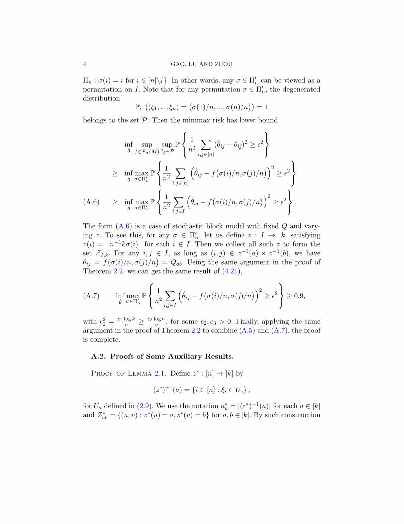
4 GAO, LU AND ZHOU
Πn : σ(i) = i for i ∈ [n]\I. In other words, any σ ∈ Π′n can be viewed as apermutation on I. Note that for any permutation σ ∈ Π′n, the degenerateddistribution
Pσ((ξ1, ..., ξn) =
(σ(1)/n, ..., σ(n)/n
))= 1
belongs to the set P. Then the minimax risk has lower bound
infθ
supf∈Fα(M)
supPξ∈P
P
1
n2
∑i,j∈[n]
(θij − θij)2 ≥ ε2
≥ infθ
maxσ∈Π′n
P
1
n2
∑i,j∈[n]
(θij − f
(σ(i)/n, σ(j)/n
))2≥ ε2
≥ inf
θmaxσ∈Π′n
P
1
n2
∑i,j∈I
(θij − f
(σ(i)/n, σ(j)/n
))2≥ ε2
.(A.6)
The form (A.6) is a case of stochastic block model with fixed Q and vary-ing z. To see this, for any σ ∈ Π′n, let us define z : I → [k] satisfyingz(i) = dn−1kσ(i)e for each i ∈ I. Then we collect all such z to form theset ZI,k. For any i, j ∈ I, as long as (i, j) ∈ z−1(a) × z−1(b), we haveθij = f
(σ(i)/n, σ(j)/n
)= Qab. Using the same argument in the proof of
Theorem 2.2, we can get the same result of (4.21),
(A.7) infθ
maxσ∈Π′n
P
1
n2
∑i,j∈I
(θij − f
(σ(i)/n, σ(j)/n
))2≥ ε2
≥ 0.9,
with ε22 = c2 log kn ≥ c3 logn
n , for some c2, c3 > 0. Finally, applying the sameargument in the proof of Theorem 2.2 to combine (A.5) and (A.7), the proofis complete.
A.2. Proofs of Some Auxiliary Results.
Proof of Lemma 2.1. Define z∗ : [n]→ [k] by
(z∗)−1(a) = i ∈ [n] : ξi ∈ Ua ,
for Ua defined in (2.9). We use the notation n∗a = |(z∗)−1(a)| for each a ∈ [k]and Z∗ab = (u, v) : z∗(u) = a, z∗(v) = b for a, b ∈ [k]. By such construction
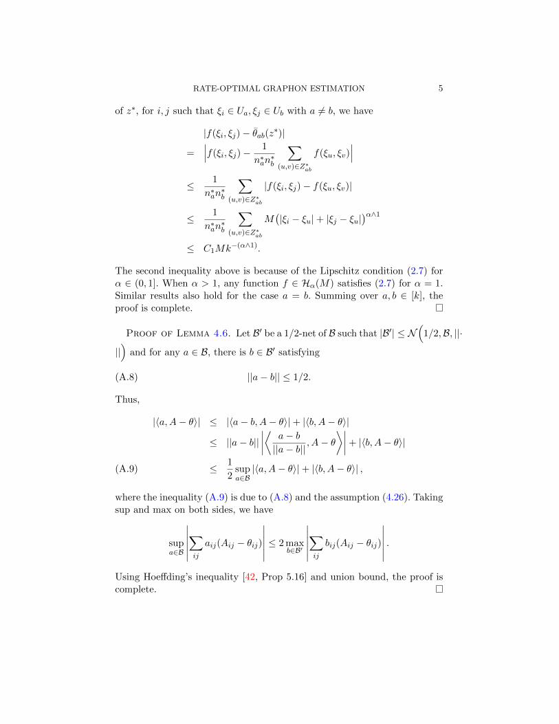
RATE-OPTIMAL GRAPHON ESTIMATION 5
of z∗, for i, j such that ξi ∈ Ua, ξj ∈ Ub with a 6= b, we have
|f(ξi, ξj)− θab(z∗)|
=∣∣∣f(ξi, ξj)−
1
n∗an∗b
∑(u,v)∈Z∗ab
f(ξu, ξv)∣∣∣
≤ 1
n∗an∗b
∑(u,v)∈Z∗ab
|f(ξi, ξj)− f(ξu, ξv)|
≤ 1
n∗an∗b
∑(u,v)∈Z∗ab
M(|ξi − ξu|+ |ξj − ξu|
)α∧1
≤ C1Mk−(α∧1).
The second inequality above is because of the Lipschitz condition (2.7) forα ∈ (0, 1]. When α > 1, any function f ∈ Hα(M) satisfies (2.7) for α = 1.Similar results also hold for the case a = b. Summing over a, b ∈ [k], theproof is complete.
Proof of Lemma 4.6. Let B′ be a 1/2-net of B such that |B′| ≤ N(
1/2,B, ||·
||)
and for any a ∈ B, there is b ∈ B′ satisfying
(A.8) ||a− b|| ≤ 1/2.
Thus,
|〈a,A− θ〉| ≤ |〈a− b, A− θ〉|+ |〈b, A− θ〉|
≤ ||a− b||∣∣∣∣⟨ a− b||a− b||
, A− θ⟩∣∣∣∣+ |〈b, A− θ〉|
≤ 1
2supa∈B|〈a,A− θ〉|+ |〈b, A− θ〉| ,(A.9)
where the inequality (A.9) is due to (A.8) and the assumption (4.26). Takingsup and max on both sides, we have
supa∈B
∣∣∣∣∣∣∑ij
aij(Aij − θij)
∣∣∣∣∣∣ ≤ 2 maxb∈B′
∣∣∣∣∣∣∑ij
bij(Aij − θij)
∣∣∣∣∣∣ .Using Hoeffding’s inequality [42, Prop 5.16] and union bound, the proof iscomplete.

6 GAO, LU AND ZHOU
Proof of Proposition 4.2. By definition,
D(Pθ||Pθ′) =∑ij
(θij log
θijθ′ij
+ (1− θij) log1− θij1− θ′ij
)
≤∑ij
(θij − θ′ij)2
θ′ij(1− θ′ij)
≤ 8∑ij
(θij − θ′ij)2,
where we using the inequality log x ≤ x− 1 for x > 0 for the first inequalityand the fact that 1/4 ≤ θ′ij ≤ 3/4 for the second inequality. We then boundthe chi-squared divergence in the same way,
χ2(Pθ||Pθ′) =∏ij
(1 +
(θij − θ′ij)2
θ′ij(1− θ′ij)
)− 1
≤ exp
∑ij
log(1 + 8(θij − θ′ij)2
)− 1
≤ exp
8∑ij
(θij − θ′ij)2
.
The proof is complete.
Proof of Proposition A.1. By the definition of K(x, y), we have
|K(x1, y1)−K(x2, y2)| ≤ 2 ||x1| − |x2|| |1− 2|y1||+ 2 ||y1| − |y2|| |1− 2|x2||≤ 2 (|x1 − x2|+ |y1 − y2|) .
For any (x1, y1), (x2, y2) in the support of φab, we have
|φab(x1, y1)− φab(x2, y2)| ≤ 2Lk1−α (|x1 − x2|+ |y1 − y2|)≤ 2L (|x1 − x2|+ |y1 − y2|)α ,
where we have used α ∈ (0, 1) and |x1 − x2| + |y1 − y2| ≤ k−1 in the lastinequality. This means φab ∈ Hα(M) for some sufficiently small L. Thisproves the first claim. For the second one, note that,∑
i,j∈[n]
φ2ab(i/n, j/n) = L2k−2α
∑i,j∈[n]
K2
(ki
n− a+
1
2,kj
n− b+
1
2
),
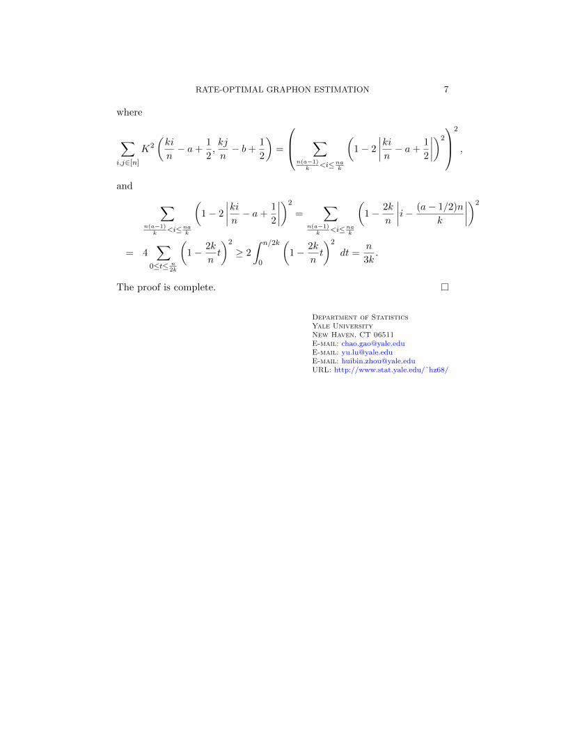
RATE-OPTIMAL GRAPHON ESTIMATION 7
where
∑i,j∈[n]
K2
(ki
n− a+
1
2,kj
n− b+
1
2
)=
∑n(a−1)
k<i≤na
k
(1− 2
∣∣∣∣kin − a+1
2
∣∣∣∣)2
2
,
and ∑n(a−1)
k<i≤na
k
(1− 2
∣∣∣∣kin − a+1
2
∣∣∣∣)2
=∑
n(a−1)k
<i≤nak
(1− 2k
n
∣∣∣∣i− (a− 1/2)n
k
∣∣∣∣)2
= 4∑
0≤t≤ n2k
(1− 2k
nt
)2
≥ 2
∫ n/2k
0
(1− 2k
nt
)2
dt =n
3k.
The proof is complete.
Department of StatisticsYale UniversityNew Haven, CT 06511E-mail: [email protected]: [email protected]: [email protected]: http://www.stat.yale.edu/˜hz68/