EXTENSIVE AND INTENSIVE INVESTMENT OVER THE BUSINESS CYCLE

by

Boyan Jovanovic and Peter L. Rousseau

Working Paper No. 09-W12

September 2009

DEPARTMENT OF ECONOMICS

VANDERBILT UNIVERSITY

NASHVILLE, TN 37235

www.vanderbilt.edu/econ

Extensive and Intensive Investment over theBusiness Cycle∗

Boyan Jovanovic and Peter L. Rousseau

May 4, 2009

Abstract

Investment of U.S. firms responds asymmetrically to Tobin’s Q: Investmentof established firms — ‘intensive’ investment — reacts negatively to Q whereasinvestment of new firms — ‘extensive’ investment — responds positively andelastically to Q. This asymmetry, we argue, reflects a difference between es-tablished and new firms in the cost of adopting new technologies. A fall in thecompatibility of new capital with old capital raises measured Q and reducesthe incentive of established firms to invest. New firms do not face such com-patibility costs and step up their investment in response to the rise in Q. Acomposite-capital version of the model fits the data well using aggregates since1900 and our new database of firm-level Qs that extend back to 1920.

1 Introduction

The distinction between the extensive and intensive margin in labor supply has beenmodeled at the individual-worker level (Cogan 1981) and at the aggregate level (Kyd-land and Prescott 1991) to understand why people move in and out of the labor marketmore wage-elastically than employed workers adjust their hours. A similar patternseems to exist for investment as well in that fluctuations in aggregate Tobin’s Q havesignificantly larger effects on the entry of firms and their investment than they do onthe investment of incumbent firms.

The investment of listed firms in the United States is unrelated or even negativelyrelated to aggregate Q. The negative relation between this ‘intensive’ investment andQ appears in investment data at both the aggregate and firm levels. In contrast, the

∗We thank G. Alessandria, W. Brainard, R. Lucas, G. Violante and L. Wong for comments, R.Tamura for data, S. Bigio, L. Han, T. Islam, M. Jaremski, J. H. Kim, K. Livingston, H. Tretvolland V. Tsyrennikov for research assistance, and the Ewing Marion Kauffman Foundation and theNSF for financial assistance.

1

investment of young and unlisted firms — ‘extensive’ investment — responds positivelyand highly elastically to Q. Inflows of venture capital in particular are highly elasticwith respect to Q, as are more noisy measures of new firms’ investment such as IPOs.

In this paper we argue that the asymmetry in investment behavior originates inthe cost of making new capital compatible with capital already in place. When newtechnology is embodied in capital, established firms will not invest in it as much asnew firms will.1 If the arrival of new technology precedes high-Q periods, then a highQ is the result of high costs of adjustment that reflect this incompatibility.

Our model is most closely related to Kydland and Prescott (1991). They assumethat people are heterogeneous in the costs of moving in and out of the labor market.We assume that new firms vary in how efficiently they can create capital. Bothmodels give rise to aggregate adjustment costs. One difference is that in our modelthe aggregate cost of adjustment is not symmetric–its convexity as induced by thedistribution of individual agents’ costs appears in the movement of new firms’ capitalinto the market, but not in its withdrawal. More generally, the model relates toothers like Cho and Rogerson (1998) and Cho and Cooley (1993) that incorporateboth the extensive and intensive margins into labor supply. But there are importantother differences: Inelastic labor of incumbent workers in all of these models stemsfrom curvature in the utility of leisure, with each additional unit forgone being moreand more valuable. The analog of such a curvature in the utility function wouldbe curvature in the incumbent firm’s production function sufficient to produce theasymmetric response.2 But this would conflict with the near Gibrat Law that one seesin the data and with the large cross-sectional variance in the size distribution of firmsseen in most industries. We therefore take a different approach, namely, to assumethat there are hidden costs of implementing new technology that only incumbentsface because they must make their old capital compatible with the new.

Compatibility costs are thus central to our model; Yorukoglu (1998) models theirimpact across steady states and finds that a fall in the compatibility of new and oldcapital raises the capital stock in young plants, lowers it in older ones, and shortensplant life. Our model extends this idea to time series as we fit it to 105 years of U.S.data. As in Greenwood, Hercowicz, and Krusell (1997) and Fisher (2006), we havetwo aggregate shocks: A TFP shock and a shock to the cost of capital, except that thelatter applies only to incumbents. We then add idiosyncratic shocks to the generationof new ideas where the number of new ideas is proportional to the stock of humancapital as in Chatterjee and Rossi-Hansberg (2008). Each period there is a qualitydistribution among the potential new projects, some of which are developed. The

1This is because new firms rely less on traditional inputs and more on new ideas, which isconsistent with Prusa and Schmitz (1991, 1994) who concluded that firms pursue less radical formsof innovation as they age.

2An extreme solution would be that of Campbell (1998) and Bilbiie et al. (2007) who assumethat the firm’s size is fixed at its entering size. Bilbiie et al in Sec. 5 briefly extend to allow variableplant size but do not study the issue of differential elasticity of extensive and intensive investment.

2

development of new projects has the interpretation of spin-outs. As do Franco andFilson (2006) and (implicitly) Prescott and Boyd (1987), we argue that incumbentfirms are able to collect the rents of the spun-out projects through lower wages thattheir workers will accept, and that the equilibrium is efficient. This means that theequilibrium solves the planner’s optimum, and this is how we shall simulate it.Evidence on investment and Q.–The patterns that we outline above can be

seen in both micro and macro data. Here we summarize that evidence, first on themicro and then on the macro side.Compustat data.–Standard and Poor’s Compustat database consists of public

firms that we think of as incumbents. The investment rate of these listed firmsdepends positively on their own Q, but negatively on aggregate Q. This is seen inFigure 1 where the vertical axes measure the log of a firm’s physical investmentsrelative to its capital stock.3 The left panel shows a mildly positive relation betweenthe investment rates of Compustat firms and their firm-specific Q’s.4 The rightpanel, on the other hand, shows a negative relation between the same Compustatfirms’ investment rates and aggregate Q, measured as the annual averages of thefirm-specific Q’s in our sample. The horizontal axis in the right panel orders theobservations by aggregate Q.The same contrast emerges in another regression that uses the Compustat data

displayed in Figure 1. Firm i’s investment as a percentage of its capital stock at datet is denoted by (I/K)i,t, aggregate Q is denoted by Qt and firm i’s deviation from itby Qi,t −Qt. The estimates and the t-ratios are

ln

µI

K

¶i,t

= 2.752(230.9)

− 0.082(−19.3)

Qt + 0.015(2.5)

(Qi,t −Qt) ,

with R2=.008 and 160,580 firm-level observations.Venture capital flows into young firms.–The only systematic source of micro

evidence on what we would regard as entering firms is Thompson’s VentureXpertsample of venture-backed firms. Venture capitalists (VCs) invest almost exclusively

3The investment rate is measured as a firm’s annual expenditures on property, plant, and equip-ment (Compustat item 30) as a percentage of its total assets at the start of the year (item 6).

4We compute firm-specific Q’s from 1962 to 2005 using year-end data from Compustat. Wemeasure the numerator of Q as the value of a firm’s common equity at current share prices (theproduct of Compustat items 24 and 25), to which we add the book values of preferred stock (item130) and long- and short-term debts (items 9 and 34). We use book values of preferred stock anddebt in the numerator because prices of preferred stocks are not available on Compustat and we donot have information on issue dates for debt from which we might better estimate market value. Wenote that book values of these components are reasonable approximations of market values so longas interest rates do not vary excessively. We compute the denominator of Q in the same way exceptthat book value of common equity (Compustat item 60) is used rather than its market value. Ourmicro-based measures of Q therefore focus primarily on the value of a firm’s outstanding securitiesand implictly assume that the proceeds from these issues are fully applied to the formation of capital,both physical and intangible.

3

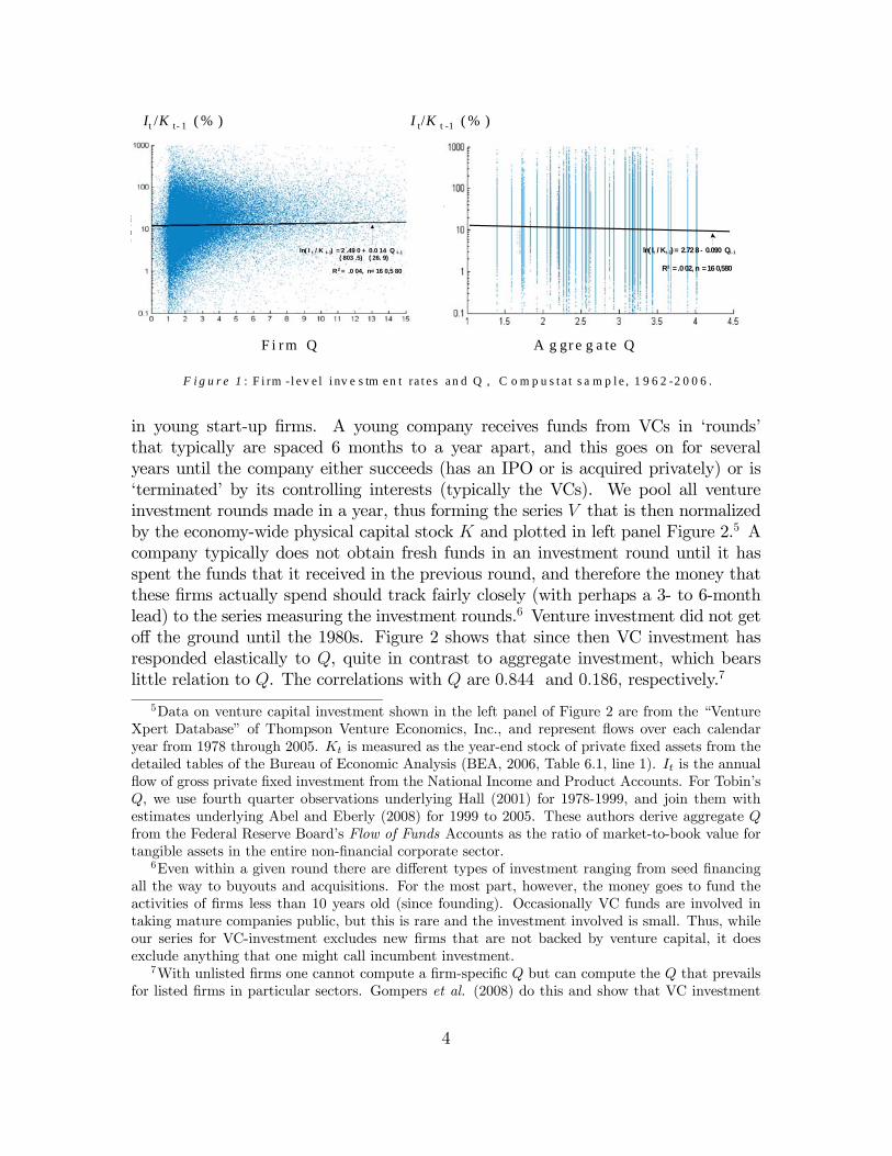
ln( I t / K t-1) = 2.728 - 0.090 Q t-1

R2 = .002, n = 160,580

Aggregate Q t (annual mean)

( 803 .5) ( 26. 9) ln( I t / K t-1) = 2 .49 0 + 0.0 14 Q t-1

R2 = .0 04, n= 16 0,5 80

F ir m Q t

A g gr e g a te QF i r m Q

It /K t- 1 ( % ) I t/K t -1 ( % )

F i g u r e 1 : F i rm -l e v e l i nv e s tm e n t ra t e s a n d Q , C o m p u s t a t s a m p l e , 1 9 6 2 -2 0 0 6 .

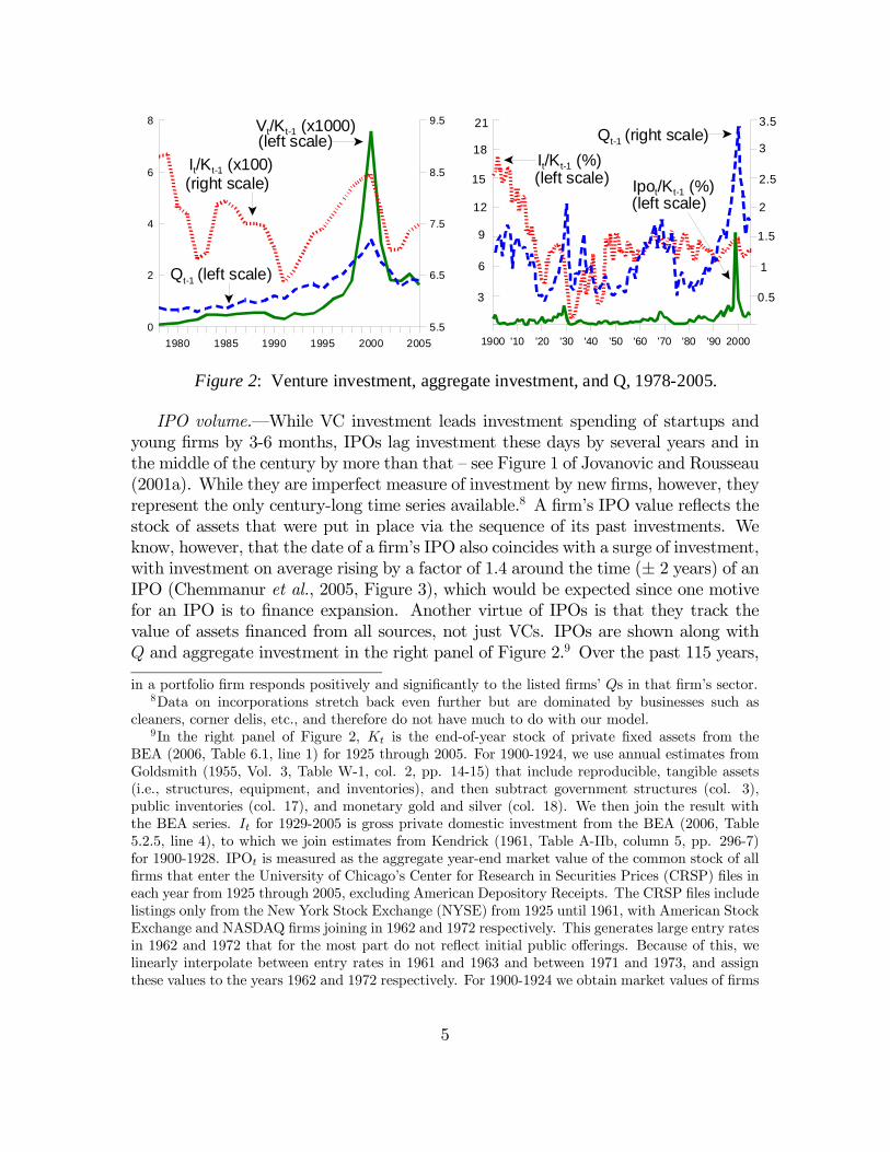
in young start-up firms. A young company receives funds from VCs in ‘rounds’that typically are spaced 6 months to a year apart, and this goes on for severalyears until the company either succeeds (has an IPO or is acquired privately) or is‘terminated’ by its controlling interests (typically the VCs). We pool all ventureinvestment rounds made in a year, thus forming the series V that is then normalizedby the economy-wide physical capital stock K and plotted in left panel Figure 2.5 Acompany typically does not obtain fresh funds in an investment round until it hasspent the funds that it received in the previous round, and therefore the money thatthese firms actually spend should track fairly closely (with perhaps a 3- to 6-monthlead) to the series measuring the investment rounds.6 Venture investment did not getoff the ground until the 1980s. Figure 2 shows that since then VC investment hasresponded elastically to Q, quite in contrast to aggregate investment, which bearslittle relation to Q. The correlations with Q are 0.844 and 0.186, respectively.7

5Data on venture capital investment shown in the left panel of Figure 2 are from the “VentureXpert Database” of Thompson Venture Economics, Inc., and represent flows over each calendaryear from 1978 through 2005. Kt is measured as the year-end stock of private fixed assets from thedetailed tables of the Bureau of Economic Analysis (BEA, 2006, Table 6.1, line 1). It is the annualflow of gross private fixed investment from the National Income and Product Accounts. For Tobin’sQ, we use fourth quarter observations underlying Hall (2001) for 1978-1999, and join them withestimates underlying Abel and Eberly (2008) for 1999 to 2005. These authors derive aggregate Qfrom the Federal Reserve Board’s Flow of Funds Accounts as the ratio of market-to-book value fortangible assets in the entire non-financial corporate sector.

6Even within a given round there are different types of investment ranging from seed financingall the way to buyouts and acquisitions. For the most part, however, the money goes to fund theactivities of firms less than 10 years old (since founding). Occasionally VC funds are involved intaking mature companies public, but this is rare and the investment involved is small. Thus, whileour series for VC-investment excludes new firms that are not backed by venture capital, it doesexclude anything that one might call incumbent investment.

7With unlisted firms one cannot compute a firm-specific Q but can compute the Q that prevailsfor listed firms in particular sectors. Gompers et al. (2008) do this and show that VC investment

4

1980 1985 1990 1995 2000 20050

2

4

6

8

5.5

6.5

7.5

8.5

9.5Vt/Kt-1 (x1000)

Qt-1 (left scale)

(right scale)It/Kt-1 (x100)

(left scale)

1900 '10 '20 '30 '40 '50 '60 '70 '80 '90 2000

It/Kt-1 (%)Ipot/Kt-1 (%)

Qt-1 (right scale)

(left scale)(left scale)

21

18

15

12

9

6

3 0.5

1

1.5

2

2.5

3

3.5

Figure 2: Venture investment, aggregate investment, and Q, 1978-2005.

IPO volume.–While VC investment leads investment spending of startups andyoung firms by 3-6 months, IPOs lag investment these days by several years and inthe middle of the century by more than that — see Figure 1 of Jovanovic and Rousseau(2001a). While they are imperfect measure of investment by new firms, however, theyrepresent the only century-long time series available.8 A firm’s IPO value reflects thestock of assets that were put in place via the sequence of its past investments. Weknow, however, that the date of a firm’s IPO also coincides with a surge of investment,with investment on average rising by a factor of 1.4 around the time (± 2 years) of anIPO (Chemmanur et al., 2005, Figure 3), which would be expected since one motivefor an IPO is to finance expansion. Another virtue of IPOs is that they track thevalue of assets financed from all sources, not just VCs. IPOs are shown along withQ and aggregate investment in the right panel of Figure 2.9 Over the past 115 years,

in a portfolio firm responds positively and significantly to the listed firms’ Qs in that firm’s sector.8Data on incorporations stretch back even further but are dominated by businesses such as

cleaners, corner delis, etc., and therefore do not have much to do with our model.9In the right panel of Figure 2, Kt is the end-of-year stock of private fixed assets from the

BEA (2006, Table 6.1, line 1) for 1925 through 2005. For 1900-1924, we use annual estimates fromGoldsmith (1955, Vol. 3, Table W-1, col. 2, pp. 14-15) that include reproducible, tangible assets(i.e., structures, equipment, and inventories), and then subtract government structures (col. 3),public inventories (col. 17), and monetary gold and silver (col. 18). We then join the result withthe BEA series. It for 1929-2005 is gross private domestic investment from the BEA (2006, Table5.2.5, line 4), to which we join estimates from Kendrick (1961, Table A-IIb, column 5, pp. 296-7)for 1900-1928. IPOt is measured as the aggregate year-end market value of the common stock of allfirms that enter the University of Chicago’s Center for Research in Securities Prices (CRSP) files ineach year from 1925 through 2005, excluding American Depository Receipts. The CRSP files includelistings only from the New York Stock Exchange (NYSE) from 1925 until 1961, with American StockExchange and NASDAQ firms joining in 1962 and 1972 respectively. This generates large entry ratesin 1962 and 1972 that for the most part do not reflect initial public offerings. Because of this, welinearly interpolate between entry rates in 1961 and 1963 and between 1971 and 1973, and assignthese values to the years 1962 and 1972 respectively. For 1900-1924 we obtain market values of firms

5

the correlation coefficient between Q and IPO value is 0.574, while the correlationbetween Q and the rate of standard investment is 0.305. Restricting the time periodto 1954-2005, the respective correlations are even further apart: 0.635 and 0.246.

2 Model

Our model allows investment to take place in new projects and in continuing projects.Continuing projects will all offer the same rate of return whereas new projects willbe heterogeneous.

Continuing projects.–Continuing projects can be enlarged at the uniform rate ofreturn 1/q. For q units of the consumption good, a unit of new capital can be createdvia existing projects. Then if the capital created via existing projects is X, the totalcost is qX.

New projects.–Many new potential projects are born each period. A projectlasts one period. It requires λ units of the numeraire good as input, and as outputit delivers ελ units of capital in the following period. Projects vary in quality; newpotential projects are born each period, and their quality is distributed with C.D.F.G (ε). In an economy with capital stock k, the unnormalized distribution of new ideasis kG (ε).10 Each period, an available project must be implemented at once or not atall. Let εm be the marginal project implemented. The size of the average project isλ. Capital created by the new projects is

Y = λk

Z ∞

εm

εdG (ε) , (1)

at a cost ofTC = λk [1−G (εm)]≡ h

¡Yk

¢k

. (2)

that list for the first time on the NYSE using our pre-CRSP database of stock prices, par values,and book capitalizations (see Jovanovic and Rousseau 2001b, footnote 1, p. 1). For Q, we use theseries derived from Hall (2001) and Abel and Eberly (2008) described in footnote 5 for 1950-2005,which we then take back to 1900 by ratio splicing the “equity Q” measure underlying Wright (2004).Note that Hall’s measure of Q exceeds Wright’s by factor of more than 1.5 in 1950, when the spliceoccurs, producing Q’s before 1950 that are considerably higher than Wright’s original estimates.10Formally, the distribution G (ε) is closely related to Kydland and Prescott (1991, p. 67) where

they model costs of moving an individual between the market and the household sector. In theirmodel, however, the cost pertained to movement in either direction, whereas here they pertain onlyto moving capital into the market sector. Retiring capital is costless, it simply can be consumed.These projects are ‘investment options’ but, in contrast to how they were modeled by Jovanovic

(forthcoming, where, as here, the supply of options was also proportional to k), they are heteroge-neous in quality, but not storable.

6

The second definition in (2) is valid because by (1), εm depends only on the ratioY/k. Therefore total cost is homogenous of degree 1 in Y and k, and we shall denoteit by h

¡Yk

¢k.

Aggregate resource constraint.–Aggregate output is zk. There is one capital good,k, but two ways to augment it: via continuing projects that deliver X, and via newprojects that deliver Y . Thus k evolves as

k0 = (1− δ) k +X + Y. (3)

The resource constraint expresses aggregate consumption as

C = zk − qX − h

µY

k

¶k. (4)

Since the form of h is fully determined by the constant λ and the distribution G, thisis a consistency condition on the macro and the micro data. Note the asymmetriceffect of q on investment costs: New projects do not require that new capital combinewith old capital, and thus escape the compatibility costs that cause q to fluctuate.11

One-sector representation.–The model has a standard one-sector representation.Let I = X + Y and let y = Y/k, x = X/k, c = C/k, and i = x+ y. Then

γ (i, q) ≡ min0≤y≤i

{q (i− y) + h (y)}

with the FOCh0 (y) = q (5)

as illustrated in Figure 3. Then (3) and (4) become

k0

k= 1− δ + i and c = z − γ (i, q) .

By the envelope theorem∂γ

∂q= x (6)

and∂γ

∂i= q if x > 0. (7)

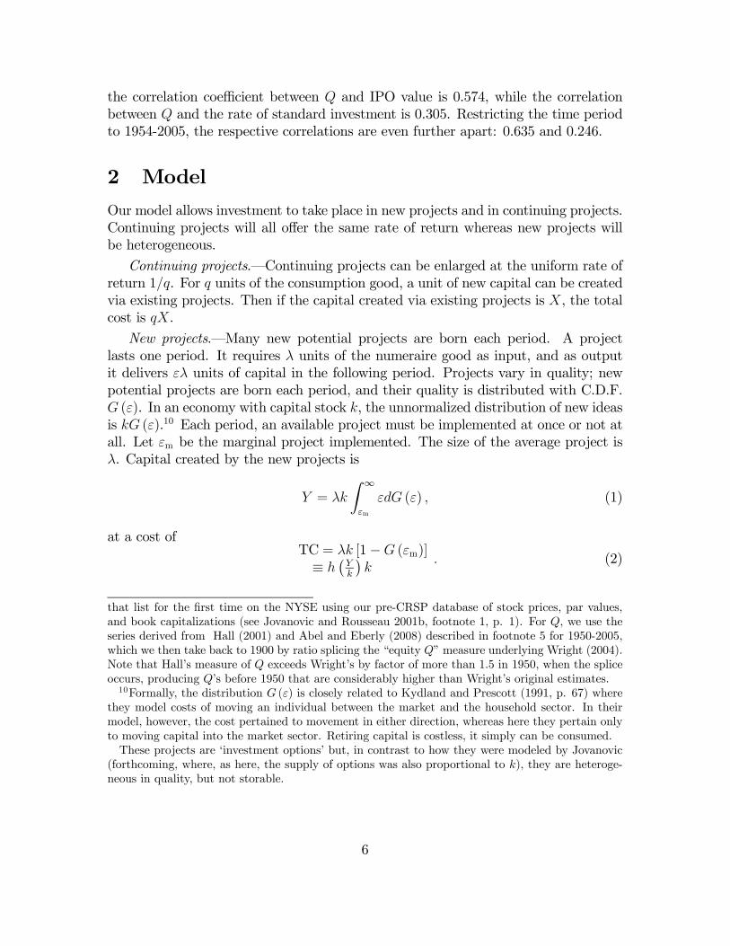
The determination of investment.–Figure 3 shows the supply of savings curve inblue. As we shall show, this curve is negatively sloped because, as seen from (4), arise in q raises the cost of future consumption in terms of current consumption

11This compatibility argument applies to physical capital and organization capital alike. Fittingnew wiring or new equipment into an old building originally designed for something else is costly.Retraining workers who originally were trained to do something else is also costly.

7

Figure 3: The determination of y via (5).

thereby reducing the demand for future consumption and reducing investment. Theinvestment rate of entering capital is fully determined by and increasing in q, as alsoshown. Incumbent investment will take up the slack between desired total investmentand the investment of entrants. There will be a second shock, z, to the supply ofsavings and, hence, the residual incumbent investment will depend on both q and z.

Figure 3 illustrates the effect of a rise in q when z is held constant. The ‘interiority’requirement that x > 0 implies that we can determine y from the intersection of theentrants’ investment-demand curve h0 (y) with q. As q rises while z stays fixed, twothings happen: First, savings declines and with it total investment i must fall from i1to i2. Second, the supply of entrants rises from y1 to y2, thereby crowding out evenmore incumbent investment.12

A rise in z, on the other hand, would shift the downward-sloping savings curve inFigure 3 to the right. This shift would cause both x and y to rise.

12These implications remain valid under a more general specification: Rewrite (4) as c = z− qx−h (y). Thus q raises the costs of incumbents but not that of entrants. Suppose, instead, that theresource constraint were c = z − qx − qψh (y) with ψ 6= 0. Then instead of (5) the FOC would beh0 (y) = q1−ψ and the conclusions illustrated in Figure 3 would remain qualitatively intact so longas ψ < 1. That is, y would be increasing in q and x would be decreasing in q. If, however, ψ = 1, ywould be a constant, independent of both q and z, and would solve the equation h0 (y) = 1. But xwould still be decreasing in q.

8

In terms of the micro interpretation of equations 1 and 2, they read

y = λ

Z ∞

εm

εdG (ε) and h (y) = λ [1−G (εm)] . (8)

Differentiating and simplifying leads to

h0 (y) =1

εmand h00 (y) =

1

ε3m

1

g (εm)> 0.

Since h is convex, (5) then implies that

εm =1

q. (9)

Thus as we raise q in Figure 3, we draw in more new projects of ever lower quality.

2.1 The planner’s problem

The economy has no external effects or monopoly power and equilibrium can berepresented by a planner’s problem. Preferences are E0

©P∞0 βtU (Ct)

ª. Let s ≡

(q, z) be stochastic with transition function F (s0, s). If technological progress raisescompatibility costs, z and q will be positively correlated. We shall therefore allow forsuch a correlation.

The state of the economy is (s, k), but since returns are constant and preferenceshomothetic, k will not affect prices or investment rates. The planner’s problem isto maximize the representative agent’s expected utility by choosing the two kinds ofinvestments X and Y . The planner has no other technology. Let preferences be

U (c) =c1−σ

1− σ,

in which case the planner’s value function must satisfy

V (s, k) = v (s) k1−σ, (10)

where

v(s) = maxi≥0

((z − γ (i, q))

1− σ

1−σ+ (1− δ + i)1−σv∗(s)

), (11)

andv∗ (s) = β

Zv (s0) dF (s0, s) .

But if z and q are positively persistent and mutually independent, v and v∗ are bothstrictly increasing in z and strictly decreasing in q.

9

The FOC with respect to y is (6) and, in light of (7), the FOC with respect to i is

q (z − γ)−σ = (1− δ + i)−σ v∗ (s) . (12)

To ensure that both FOCs hold with equality, we assume that h (0) = 0, whichrules out the value y = 0, and that h0 (y) > qmax at a value of y too low to satisfy thedemand for saving in any state s, which rules out x = 0.We may rearrange (12) to obtain

i = δ − 1 + (z − γ)

µv∗

q

¶1/σ(13)

and we at once have the following properties of x, y, and i:

1. y is increasing in q and independent of z, these follow from (5); and

2. i and x are decreasing in q and increasing in z. The claims about i follow from(6) and (13), and the claims about x then follow from property 1.

2.2 Decentralization

Although established firms find it harder than new firms to adopt technology, they dobuild new plants and start new ventures. Interestingly, however, when they do so, theyestablish semi-independent divisions. Gompers (2002, esp. table 6) and Dushnitskyand Shapira (2006) survey corporate VC activity. Nevertheless, implementing newideas often requires that an employee leave the firm — a spinout. The microfoundationsof spin-outs involve asymmetric information. Klepper and Thompson (2006) arguethat spin-outs occur because people disagree over management decisions — peopleleave firms to develop their ideas on their own because coworkers would otherwiseimplement them suboptimally. Chatterjee and Rossi-Hansberg (2008) argue that thebest ideas leave the firm. Finally, Franco and Filson (2006) argue that a firm’s span-of-control limit pushes some of its employees out to start their own firms using trainingthey received on the job. The models differ, but they all treat entry essentially as awithdrawal of capital from existing firms, and that is also how we shall treat it.We follow Prescott and Boyd (1987) and Franco and Filson (2006) and assume

that workers accept lower pay in return for what they learn. Then kG (ε) is thedistribution of idea qualities that a firm’s workers generate. Since the firm capturesthe rents via the lower wages that it pays, this gives it the correct accumulationincentives. X is the new capital that will stay in the firm and q is its unit costcommon to all incumbents, while Y is developed by workers who leave, with h0 (y)the marginal cost of doing new things and with new ideas varying in quality.13 The13New opportunities for incumbents appear to be homogeneous relative to those of new firms:

Dahlin et al. (2004) find that the variance in patent quality is higher among patents granted toindependent inventors than it is among patents granted to corporations, and that inventions in theright tail of the quality distribution are more likely to originate with independent inventors.

10

best ideas are exploited first, hence h0 is upward sloping. We now formalize thisdecentralization.

A firm’s decision problem.–The firm maximizes its value. Since its k is predeter-mined, this amounts to maximizing the unit value of k which we define as w. It takesas given the next-period value of its capital, its ex-dividend unit value today beingq. The firm’s maximization problem is then

w (s) = maxi≥0

{z − γ (i, q) + (1− δ + i) q} . (14)

This means that the firm’s y must solve (5), but x must be obtained from the house-hold savings decision and the identity that savings = investment = x+ y. The lineartechnology for creating k yields no rents because the market price of capital adjuststo equal the average and marginal cost of creating it, q. In other words, x generatesno rents. Since i = x+ y, (14) reduces to

w (s) = z + q (1− δ) + maxy{qy − h (y)} . (15)

More explicitly, each unit of k entitles the firm to some new projects each period,and the firm’s employees will spin out all those for which ε ≥ εm = 1/q as derived in(9).

The household’s budget constraint.–For a household, the only asset is shares offirms as in Lucas (1978). Firms distribute their profits to households, as well as therevenue from shares issued net of investment costs. Let the dividend be D (q, z) pershare. The household’s constraint is

qn0 + c = (D (q, z) + q)n,

where n is the number of units of capital of the representative firm that the householdowns and where c = C/k. It is helpful to write c as

c = (D − q∆)n,

where

∆ =n0 − n

n

is the household’s rate of investment in the ownership of capital.

The household’s Bellman equation.–The household’s state is (n, s). Exactly par-allel to the planner’s case, the household’s lifetime value can be written as ψ (s)n1−σ,where ψ (s) solves the Bellman equation

ψ (s) = max∆

((D (q, z)− q∆)1−σ

1− σ+ (1 +∆)1−σ ψ∗ (s)

), (16)

11

and where

ψ∗ (s) = β

Zψ (s0) dF (s0, s) .

Assuming differentiability of v and using the envelope theorem, the FOC is

q (D + q∆)−σ = (1 +∆)−σ ψ∗ (s) . (17)

Equilibrium.–We state the equilibrium conditions per unit of capital. We startwith the household owning all the capital, i.e., n = k. The rate at which the householdgrows its ownership of shares should equal the rate at which the firm grows its capitalstock. Firms finance capital expansion by issuing i− δ new shares which the publicmust choose to buy:

∆ = i− δ.

Firms’ dividends equal their net revenue from all sources, which is profits plus therevenue from newly issued shares:

D = z − γ (i, q) + q (i− δ) .

If these two conditions are met, consumption will equal output net of investment

D + q∆ = z − γ.

Equilibrium and planner’s optimum coincide.–Substituting this information into(17) leads to

q (z − γ)−σ = (1− δ + i)−σ ψ∗ (s) . (18)

From (12) we see that equilibrium and the optimum coincide if and only if v∗ (s) =ψ∗ (s) for all s. Now, if we substitute into (16) from the equilibrium conditions for Dand ∆ we obtain

ψ (s) =(z − γ (i, q))1−σ

1− σ+ (1− δ + i)1−σ β

Zψ (s0) dF (s0, s) ,

which is the same as the expression that v (s) solves, from which we conclude thatψ (s) = v (s) for all s, which means that ψ∗ (s) = v∗ (s) for all s.

3 Estimating G (ε)

A cornerstone of the model as shown in equations (1) and (2) is the distribution G (ε)of new ideas. In this section we estimate G (ε) using micro-level data from 1920 to2005 on the Q’s of IPO-ing and incumbent firms that we obtained from Compustat

12

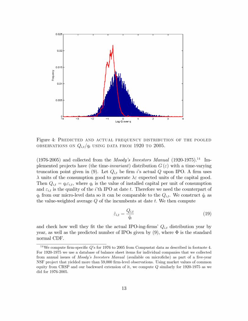
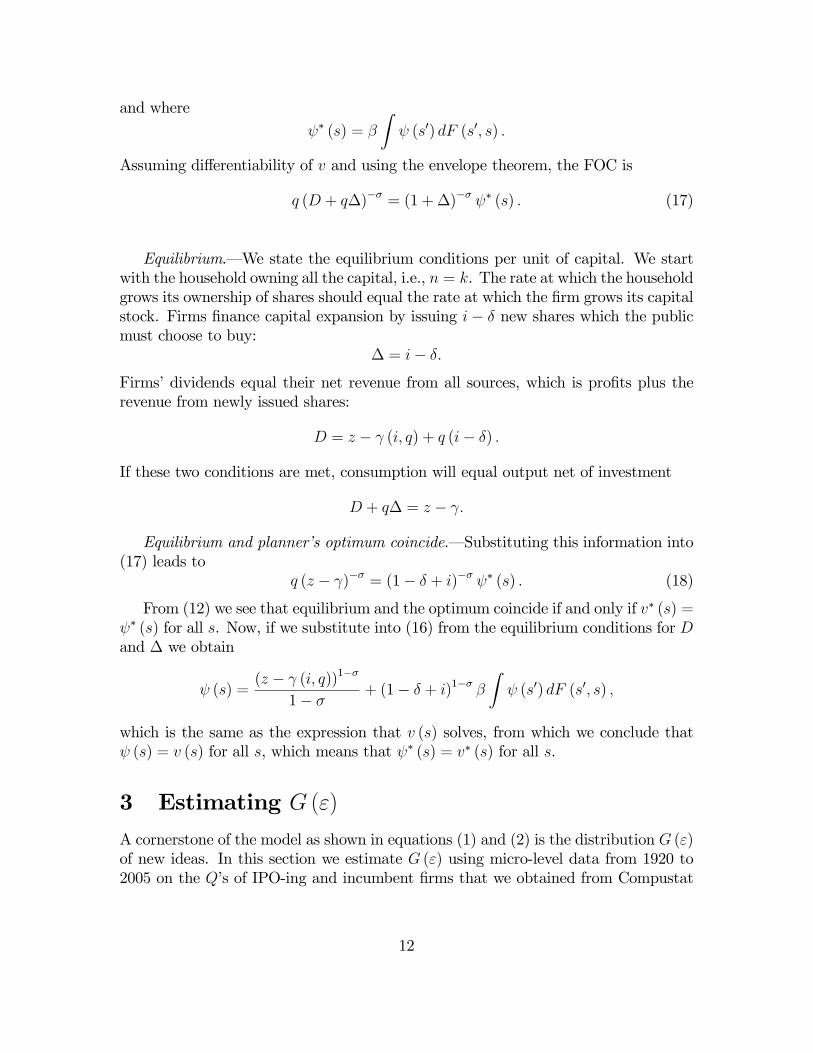
Figure 4: Predicted and actual frequency distribution of the pooledobservations on Qi,t/qt using data from 1920 to 2005.

(1976-2005) and collected from the Moody’s Investors Manual (1920-1975).14 Im-plemented projects have (the time-invariant) distribution G (ε) with a time-varyingtruncation point given in (9). Let Qi,t be firm i’s actual Q upon IPO. A firm usesλ units of the consumption good to generate λε expected units of the capital good.Then Qi,t = qtεi,t, where qt is the value of installed capital per unit of consumptionand εi,t is the quality of the i’th IPO at date t. Therefore we need the counterpart ofqt from our micro-level data so it can be comparable to the Qi,t. We construct qt asthe value-weighted average Q of the incumbents at date t. We then compute

εi,t =Qi,t

qt(19)

and check how well they fit the the actual IPO-ing-firms’ Qi,t distribution year byyear, as well as the predicted number of IPOs given by (9), where Φ is the standardnormal CDF.

14We compute firm-specific Q’s for 1976 to 2005 from Compustat data as described in footnote 4.For 1920-1975 we use a database of balance sheet items for individual companies that we collectedfrom annual issues of Moody’s Investors Manual (available on microfiche) as part of a five-yearNSF project that yielded more than 59,000 firm-level observations. Using market values of commonequity from CRSP and our backward extension of it, we compute Q similarly for 1920-1975 as wedid for 1976-2005.

13

Figure 5: Predicted and actual IPO distributions in a trough year anda peak year.

The predicted frequency distribution of all the 1920-2005 observations (weighted

each year by Nt) is

Ã2005X

t=1920

Nt

!−1 2005Xt=1920

Ntp³Qqt| qt´. Figure 4 plots the predicted

and actual frequency distributions of ln εi,t pooled over t.

The estimated g (ε) is (i) to the left of the distribution of the pooled CompustatIPO-based εt distribution and (ii) less dispersed. Let’s discuss why each of thesedeviations arises. (i) The contribution to IPO value (which is how we measure Y ) ofIPOs of a quality-level ε is value times the number of IPOs, i.e., εg (ε). The peak ofthe product εg (ε) occurs to the right of the model of g, at με + σ2ε = −1.14 and itsdistribution is slightly right skewed. It is most responsive to q at a value to the rightof the mean of ε and this is why the macro-based estimate of g (ε) places the meanof ε to the left of the mean of the data. (ii) The distribution of the Qi,t is somewhattoo dispersed to produce an adequate crescendo of implementations as aggregate qrises from unity to 3.4 as the aggregate data require. On the other hand, consideringthe small number of parameters, the model captures individual-year IPO distributionsquite well. We consider a trough year, 1982, when q1982 = 2.36, and a peak year, 2000,when q2000 = 4.48. Then since Q ≥ 1, (19) implies that ln ε1982 ≥ − ln 2.36 = −0.86and ln ε2000 ≥ − ln 4.48 = −1.5. This is shown in Figure 5.

14

4 Fitting the model to data

In our model, q is driven by hidden implementation costs. When we come to thedata, this will mean that q represents a shock relative to the price of capital thatthe BLS measures and uses to construct its estimated stock of capital. Thereforemeasured Q equals the model’s q. When compatibility problems cause reproductioncosts of incumbents to rise, this will not enter their book values (i.e., the denominatorof measured Q), and this generates a measurement error that raises measured Q.The model normalizes the measured cost of capital to unity, which means that weimplicitly assume that the price index for capital goods is correctly used by the BLSwhen constructing the capital stock numbers that we shall use here.

4.1 Construction of composite capital and other aggregates

Figure 2 does not measure the same concept for entrants as it does for incumbents.In both panels, the series I is aggregate investment in physical capital. On the otherhand, the series Vt/Kt−1 and IPOt/Kt−1 in Figure 2 track a broader concept ofinvestment.

Some of the money that VCs spend goes on plant and equipment, but the rest isused to pay rent on office space, and on salaries, raw materials, etc. Similar remarksapply to the IPO series which measures the market value of firms entering the stockmarket, i.e., and that value reflects all the assets that those firms own, not just theirphysical capital.

Since we have no measures of physical-capital creation by entrants, we shall con-struct measures of composite-capital investment for incumbents (i.e., that reflect bothphysical and human capital components) and thereby put the comparison on anequal footing by measuring the investment of both groups in the same units. Thecomposite-capital construction will tell the same story as did physical capital: Com-posite investment is unresponsive to Q whereas the composite investment of entrantsresponds elastically.

To fit the model’s implications we shall need to measure q, z, X, and Y , and toconstruct k. The specification will need to satisfy the conditions that Hayashi andInoue (1992, ‘HI’) display in their equations (2.8) and (2.11). Let k now denote thecapital composite and let k0 denote its next-period value. Aggregate consumption is

c = zk − qξ (k0 − (1− δ) k) + h

µ(1− ξ)

k0 − (1− δ) k

k

¶k,

where ξ is the fraction of investment going to incumbents. This is the analogueof HI’s profit function. Thus HI’s condition (2.8) that profits depend only on theaggregate capital stocks k and k0 is met, as is their degree-one-homogeneity condition(2.11). We retain (3) where X and Y now denote incumbent and entering investment

15

spending on broad capital. Letting m ≡ k0

k− 1 denote the growth rate of aggregate

capital, the decentralization (14) then reads

w = maxξ,m

{z − qξm− h ([1− ξ]m) + q (1 +m)} .

The FOC with respect to ξ reads

q = h ([1− ξ]m) . (20)

Then (20) is the same as (5) since y = (1− ξ)m. We now describe how we define andmeasure X and Y in the two-capital case and then use this composite-capital seriesto simulate the model.

We shall present the aggregation at the level of the price-taking firm and not atthe level of the entire economy, similar to HI. The aim is to reduce the two-capitalproblem to the one-capital version stated in (14). Assume that k is the followingaggregate of physical capital K and human capital H:

k = φ (K,H) . (21)

The aggregator φ corresponds to the aggregator φ in HI’s (2.8). The two capitalstocks evolve as follows

K 0 = (1− δ)K + IK and H 0 = (1− δ)H + IH . (22)

Each type of investment decomposes into two types

IK = XK + YK and IH = XH + YH (23)

and the total cost of the combined investment isXi∈{K,H}

pi

µqtXi + hi

µYik

¶k

¶,

where hK and hH are the non-linear portions of the adjustment cost for K and H.Let

C (q, IK , IH) = min(Xi,Yi)i∈{K,H}

Xi∈{K,H}

pi

µqXi + hi

µYik

¶k

¶, s.t. (23). (24)

If pK and pH are constant, the states are (s,K,H) where s = (z, q).15 Then letting

15Implicitly we assume that whatever gives rise to the fluctuations in the K/H ratio over timedoes not cause the efficiency prices to change. If (pK , pH) were to change over time, we would needto add more states to the analysis, and the planner too would have additional states in the problemstated in Section 2.1.

16

r (s) be the interest rate in state s, a risk-neutral firm’s value would be16

W (s,K,H) = maxK0,H0

½zφ (K,H)− C (q,K 0 − (1− δ)K,H 0 − (1− δ)H)

+ 11+r(s)

RW (s0,K 0,H 0) dF (s0, s) .

¾. (25)

We now derive conditions under which the two-capital decision problem of a firmreduces to (14). As HI do, we too can break the maximization problem into twostages: The dynamic problem of choosing the scalar aggregate k over time, and thestatic problem of choosing K and H to minimize the total input cost subject to (21).Ignoring the proportionality constant define

C (K,H, k0) = minK0H0

C (q,K 0 − (1− δ)K,H 0 − (1− δ)H) s.t. φ (K 0, H 0) ≥ k0.

(26)

Lemma 1 Ifφ (K,H) = KαH1−α

and if the optimal XK and XH are positive17 the solution to the problem in (26) is

K 0 = λα

pKk0 and H 0 = λ

1− α

pHk0 (27)

where

λ =³pKα

´αµ pH1− α

¶1−α. (28)

Since (27) and (28) also hold for (k,K,H), we let c (q, k, k0) = C³λ αpKk, λ1−α

pHk, k0

´.

Then sinceW is homogeneous of degree one in (K,H) ,we haveW³s, λ α

pKk, λ1−α

pHk´≡

w (s) k. Then the maximization problem (25) becomes

w (s) k = maxk0

½zk − c (q, k, k0) +

k0

1 + r (s)

Zw (s0) dF (s0, s)

¾= max

k0{zk − c (q, k, k0) + qk0} (29)

16We shall in fact need to assume a trend in pH relative to pK which, to keep the notation simple,we shall ignore for the moment, but which eventually we shall bring into the calculated stock of h.If pH has no trend,

ht =∞Xs=0

(1− δ)sIH,t−spH

,

whereas if pH varies according to pH,t = pH (1 + gH)t, the true stock would be

ht =∞Xs=0

µ1− δ

1 + gH

¶sIH,t−spH

.

We shall infer below that gH =0.0155.17This is a restriction on the Xi that parallels the development in Section 2 where we assumed

that the optimal X is positive for all (z, q) . This will be true when h is steep enough, as portrayedin Figure 3.

17

because arbitrage over X forces r (s) to satisfy the equation MCX = ACX = q =marginal revenue from an additional unit of X, i.e.,

q =1

1 + r (s)

Zw (s0) dF (s0, s) .

The firm therefore draws a zero return on all its units of XK and XH . Its rents derivefrom output zk, from the future value of the undepreciated portion (1− δ) k, andfrom the inframarginal units of YK and YH . Substituting into (29) and dividing by kwe get

w (s) = z + q (1− δ) +X

i∈{K,H}

(qyi − pihi (yi)) ,

where the yi = Yi/k solve the problem in (24). In order that w (s) = w (s), we musthave X

i∈{K,H}

(qyi − pihi (yi)) = maxy{qy − h (y)} ,

which works if there are constants θK and θH summing to one such that the marginalconditions to the problem in (24) are also met at yi = θiy whenever h0 (y) = q. This

is true, e.g., if we choose hi as follows: hi (yi) = θipih³

yθi

´. In that case w (s) = w (s),

and k as defined in (21) and k0 as generated via the choice of (K 0, H 0) by the problem(25) are the same as the solutions that emerge in the problem defined in (14).

Generating the series k.–The definition (21) defines composite capital to bea function of K and H, and we now describe how these series were obtained and howthey were combined into the index k, as well as how the investments x and y werecalculated.

The series K.–The aggregate physical capital stock Kt is defined as the year-end stock of private fixed assets (see footnote 9). Then from (22) we calculate It =Kt+1 − (1− δ)Kt. Both Kt and It are nominal series.

The series H.–We obtained raw data on educational achievement in the UnitedStates from worksheets underlying Turner et al. (2007). This source provided thenumber of low-skill and high-skill agents from 1901 to 2000, which we define as NU,t

and NS,t. Our skill premium series is wS,twU,t

, where wU,t and wS,t are wages per person

at date t.18 We then calculate the real stock of human capital HRt ≡ NU,t +

wS,twU,t

NS,t,

and then convert HRt into nominal units by multiplying it by Pt (in our case the CPI)

to get Ht ≡ PtHRt .

Imposing stationarity on the capital-output ratio.–We have no direct informationon the unit price of h. Since we have assumed that pK/pH is constant and since the

18Since the numbers of high- and low-skilled individuals ends in 2000 and their wage ratios end in1995, we use the average annual growth rates of each over the proceeding five years to bring theseseries forward to 2005.

18

k and the h series are already in nominal units, we shall infer the change in the unitprice of h over the century. We want our shock z to have no trend. Since Kt grows asfast as output, we adjust the average growth of H by gH as explained in footnote 16,which is the exact amount needed to ensure that it grows as fast as the K series overthe century.19 We call the resulting series Ht. We calculate IH,t from the H series as

IH,t = Ht+1 − (1− δ)Ht. (30)

Moreover the series k obtained via (21) was normalized by a multiplicative constantto fit the average output-capital ratio.Decomposing k into incumbent and entering investment.–In (3) we set X =

XH +XK and Y = YH + YK, and we then define

IH = XH + YH and IK = XK + YK

to be composite investment by incumbents and entrants. We assume that the ratioX/Y is the same for physical and for human capital. That is,

XK

YK=

XH

YH.

Then given data on the Xi and Yi, we can then calculate

x =XK +XH

kand y =

YK + YHk

.

The series for Y .–We cannot measure YH and YK separately, only their sum Y .We entertain two measures for Yt that correspond to the series plotted in Figure 2where the data sources are described as well. The first is total investment of venturecapital funds and the second measure of Y is the real value of IPOs. IPO valuesrelative to the capital stock are qy. This is the value of the composite capital stockbrought into the stock market. Division by q yields y.Calculating z.–Since output is zk, we measure z by the ratio of private output

over the course of a given year to private capital at the start of that year.20 Havingobtained composite k, we then set zt = GDPt/kt for all t.

19Thus we first obtain the average growth differential over the century by solving for gH theequation

H2005

H1900

e105gH =K2005

K1900.

We then defineHt = Hte

(t−1900)gH .

This adjustment, for which gH turns out to be 0.0155, ensures that Y/k = z is trendless.20Private output, defined as gross domestic product less government expenditures on consumption

and investment, are from the Bureau of Economic Analysis (2006) for 1929-2005, to which wejoin Kendrick’s (1961, Table A-IIb, pp. 296-7, col. 11) estimates of gross national product lessgovernment.

19

Calculating q.–In light of (14), we measure q by Tobin’s Q. The source of theQi,t for the IPOs and of qt for the established firms that we used to estimate the dis-tribution G (ε) of new ideas (in Section 3) was the Compustat data and our backwardextension of it. We use the micro Qs to estimate G (ε) because the Qs of the IPOsare also from the micro data. It turns out, however, that the Compustat-based qtexceeds the aggregate q displayed in Figure 2 by a factor of 2.4 and that the ratio ofthe two time series is trendless.21 We therefore we generate y and h via (5) and (8)by using qt ≡ (2.4) qt, where qt is the aggregate series for the entire century.The price-earnings ratio.–We also fit the economy-wide price-earnings ratio.22

Assuming that (1− α) k goes to labor compensation, earnings are αzk and therefore

PriceEarnings

=q

αzk.

4.2 Simulations of the model

We simulate the model over two time periods: 1901-2005 and 1978-2005. Parameterswere chosen to be close to conventionally used values of β, δ, and σ while still fittingthe historical averages of the rate of growth of output, investment by incumbent firmsand entering firms respectively, and the price-earnings ratio. The simulations for bothtime periods were computed using the same set of parameters with the exception ofλ, which changes because we use IPO investment for y over the 1901-2005 period andan alternate data series (i.e., VC investment) for 1978-2005. We assume that G (ε)is the log-normal distribution, with ln ε ∼ N (με, σ

2ε) which, together with λ, yields

h (y) via (8). Table 1 reports the parameter values:

Table 1: Parameter values used

β δ σ με σε λ1901-2005 λ1978-2005 α0.95 0.065 4 -1.28 0.37 0.02 0.01 0.33

21The difference arises for two reasons. First, Compustat and our backward extension only coverfirms that are listed on organized stock exchanges, while the aggregate measures of Q cover the entirenon-financial corporate sector. Our sample is thus focused on larger and more successful firms.Second, our measure of Q is based on market and book values of a firm’s outstanding securitiesissues (see footnote 4), the proceeds of which are spent on physical capital and intangibles, while theaggregate measures reflect the holding of tangible capital only. Since intangibles probably form animportant part of the forward-looking component of stock prices and our decentralization suggeststhat employees accept lower pay to develop human capital, our concept of Q would be expectedto generate higher measured values than those based upon tangibles alone. The micro-based andmacro series for Q are highly correlated with ρ = 0.92 and their ratio does not vary much over thecentury, being 2.0 in 1921 and 2.2 in 2005.22We obtain the economywide price-earnings ratio from worksheets underlying Shiller (2000),

updated through 2005 and available from his website.

20

1900 '10 '20 '30 '40 '50 '60 '70 '80 '90 2000

y (right scale)

0

0.1

0.045

model

0.03

0.015

0.2

0.3

0

data

x (left scale)model

data

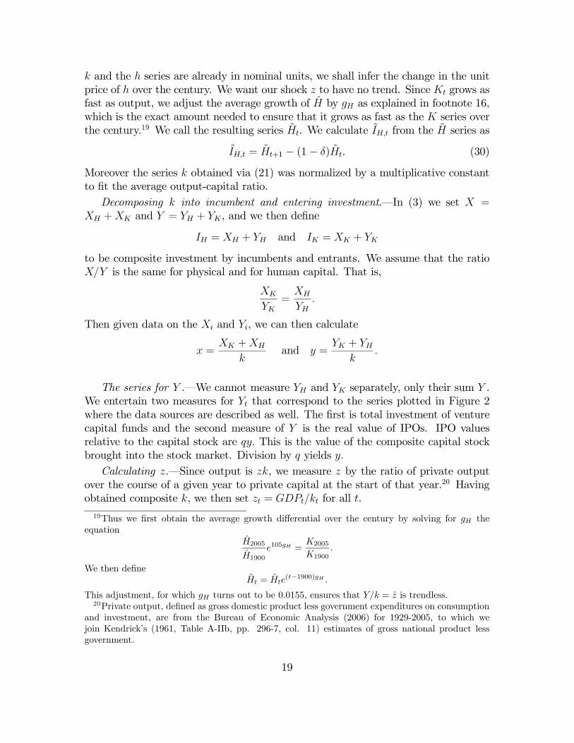
Figure 6: The Y and X series and their simulated values (with compos-ite capital), 1901-2005.

1900 '10 '20 '30 '40 '50 '60 '70 '80 '90 20000

10

20

30

40

50

P/E (model)

P/E (data)

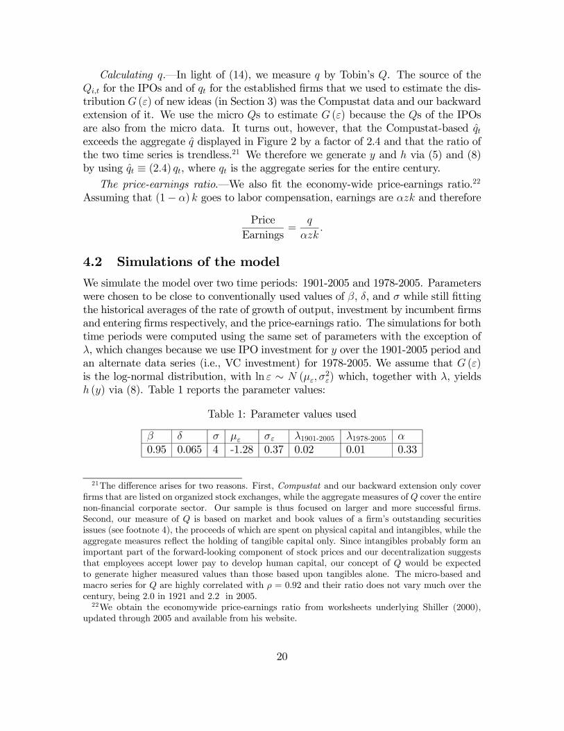
Figure 7: The price-earnings ratio and its simulated values, 1901-2005.

21

1980 1985 1990 1995 2000 2005

y (right scale)

0

0.1

0.008

model

0.006

0.004

0.002

0.2

0.3

0.4

0

data

x (left scale)

model

data

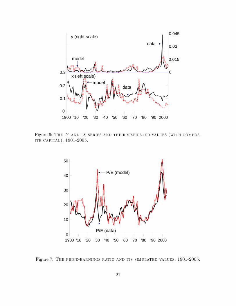
Figure 8: The Y and X series and their simulated values (with compos-ite capital), 1978-2005.

1980 1985 1990 1995 2000 20050

10

20

30

40

50P/E (model)

P/E (data)

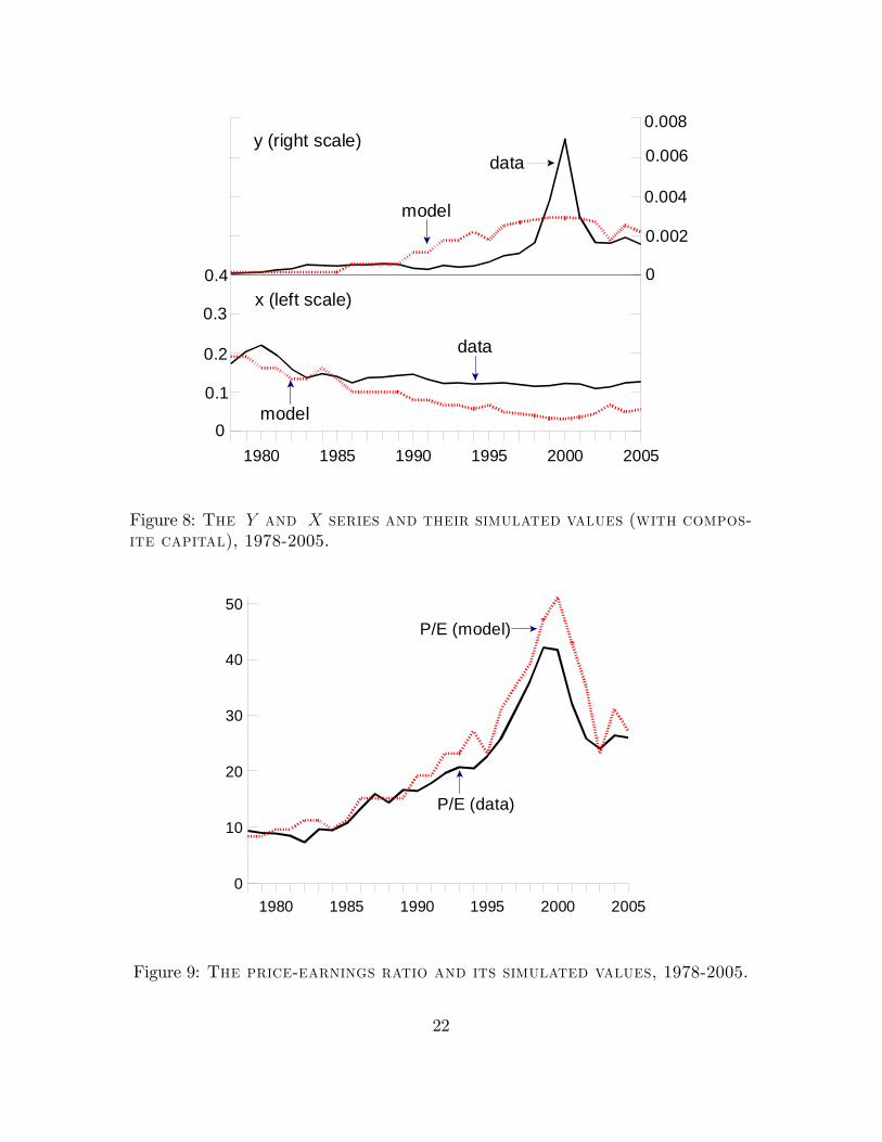
Figure 9: The price-earnings ratio and its simulated values, 1978-2005.

22

A cornerstone of the model is h (y), and given the values of με, σ2ε and λ we obtain

an S-shaped supply curve of new projects as a function of q.

The model’s predictions were generated by solving the planner’s problem usingthe discretized (z, q) process obtained from the Tauchen-Hussey procedure applied tothe data on q and z that we constructed using the procedures outlined in Section 4.1.

Simulation results for 1901-2005.–Figure 6 plots the model predictions and thedata for 1901-2005. It has in the past been notoriously difficult to explain aggregateinvestment — we remind the reader that highly successful as it is, the RBC approachremoves the HP trend and so takes the low-frequency variation in the data out. Yetthe fit of our model seems to be quite close. The y series fits well too, except thatwe do not match all of the extreme spikes in the data. Roughly speaking, there istoo much cross-sectional dispersion in Qi,t to allow the model to capture the late-90sspike, though it does quite well with the one in the late 60s. Figure 7 plots theprice-earnings ratio for the data and model and here the fit is quite good too.

Simulation results for 1978-2005 .–The only data change here is the use of theVC-investment series in place of IPOs. The model parameters are the same as for1901-2005 (see Table 1), except that λ is smaller. The latter is not surprising becauseVC investment is smaller than the IPO series. We also use the same values for z aswe used for 1901-2005. The approximation is not as good due to the large drop in zat the start. Figure 8 plots the model prediction and the data for 1978-2005, whileFigure 9 plots the price-earnings ratios. Again the fit is fairly close, but not as closeas it is for the century as a whole.

4.3 Other evidence

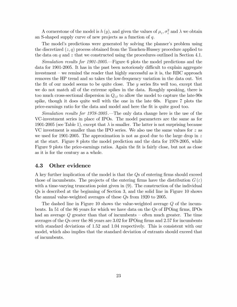
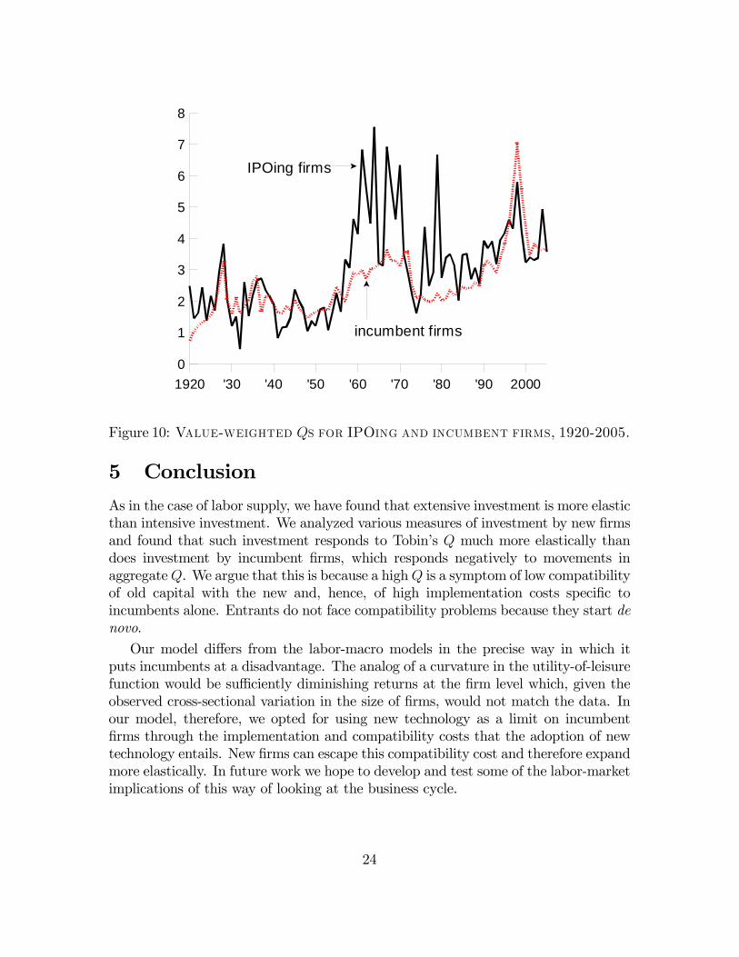
A key further implication of the model is that the Qs of entering firms should exceedthose of incumbents. The projects of the entering firms have the distribution G (ε)with a time-varying truncation point given in (9). The construction of the individualQs is described at the beginning of Section 3, and the solid line in Figure 10 showsthe annual value-weighted averages of these Qs from 1920 to 2005.

The dashed line in Figure 10 shows the value-weighted average Q of the incum-bents. In 51 of the 86 years for which we have data on the Qs of IPOing firms, IPOshad an average Q greater than that of incumbents — often much greater. The timeaverages of the Qs over the 86 years are 3.02 for IPOing firms and 2.57 for incumbentswith standard deviations of 1.52 and 1.04 respectively. This is consistent with ourmodel, which also implies that the standard deviation of entrants should exceed thatof incumbents.

23

1920 '30 '40 '50 '60 '70 '80 '90 20000

1

2

3

4

5

6

7

8

IPOing firms

incumbent firms

Figure 10: Value-weighted Qs for IPOing and incumbent firms, 1920-2005.

5 Conclusion

As in the case of labor supply, we have found that extensive investment is more elasticthan intensive investment. We analyzed various measures of investment by new firmsand found that such investment responds to Tobin’s Q much more elastically thandoes investment by incumbent firms, which responds negatively to movements inaggregateQ. We argue that this is because a highQ is a symptom of low compatibilityof old capital with the new and, hence, of high implementation costs specific toincumbents alone. Entrants do not face compatibility problems because they start denovo.

Our model differs from the labor-macro models in the precise way in which itputs incumbents at a disadvantage. The analog of a curvature in the utility-of-leisurefunction would be sufficiently diminishing returns at the firm level which, given theobserved cross-sectional variation in the size of firms, would not match the data. Inour model, therefore, we opted for using new technology as a limit on incumbentfirms through the implementation and compatibility costs that the adoption of newtechnology entails. New firms can escape this compatibility cost and therefore expandmore elastically. In future work we hope to develop and test some of the labor-marketimplications of this way of looking at the business cycle.

24

References

[1] Abel, Andrew B., and Janice C. Eberly. “How Q and Cash Flow Affect Invest-ment without Frictions: An Analytic Explanation.” Mimeo, Wharton School,University of Pennsylvania, November 2008.

[2] Bilbiie, Florin, Fabio Ghironi, and Marc Melitz. “Endogenous Entry, ProductVariety, and Business Cycles.” Working Paper No. 13646, National Bureau ofEconomic Research (November 2007).

[3] Campbell, Jeffrey. “Entry, Exit, Embodied Technology, and Business Cycles.”Review of Economic Dynamics 1, no. 2 (April 1998): 371-408.

[4] Carter, Susan B. et al. Historical Statistics of the United States: Earliest Timesto the Present.Millennial Edition. New York: Cambridge University Press, 2006.

[5] Chatterjee, Satyajit, and Esteban Rossi-Hansberg. “Spin-offs and the Market forIdeas.” Mimeo, 2008.

[6] Chemmanur, Thomas, Shan He, and Debarshi Nandy. “The Going Public Deci-sion and the Product Market.” Mimeo, Boston College, May 2005.

[7] Cho, Jang-Ok and Thomas F. Cooley. “Employment and Hours over the BusinessCycle.” Journal of Economic Dynamics and Control 18, no. 2 (March 1994):411-432.

[8] Cho, Jang-Ok and Richard Rogerson. “Family Labor Supply and Aggregate Fluc-tuations.” Journal of Monetary Economics 21, no. 2-3 (March-May 1988): 233-245.

[9] Cogan, John. “Fixed Costs and Labor Supply.” Econometrica 49, no. 4 (July1981): 945-963.

[10] Compustat database (New York: Standard and Poor’s Corporation, 2008).

[11] CRSP database (Chicago: University of Chicago Center for Research on Securi-ties Prices, 2007).

[12] Dahlin, Kristina, Margaret Taylor, and Mark Fichman. “Today’s Edisons orWeekend Hobbyists: Technical Merit and Success of Inventions by IndependentInventors” Research Policy 33, no. 8 (October 2004): 1167-1183.

[13] Dushnitsky, Gary, and Zur Shapira. “Entrepreneurial Finance Meet CorporateReality: Comparing Investment Practices by Corporate and Independent Ven-ture Capitalists.” Mimeo, NYU Stern School of Business, August 2007.

25

[14] Fisher, Jonas. “The Dynamic Effects of Neutral and Investment-Specific Tech-nology shocks.” Journal of Political Economy 114, no. 3 (June 2006): 413-451.

[15] Franco, April M., and Darren Filson. “Spin-outs: Knowledge Diffusion throughEmployee Mobility.” Rand Journal of Economics 37, no. 4 (Autumn 2006): 841-860.

[16] Goldsmith, Raymond W. A Study of Savings in the United States. Princeton,NJ: Princeton University Press, 1955.

[17] Gompers, Paul. “Corporations and the Financing of Innovation: The CorporateVenturing Experience.” FRB Atlanta Economic Review (Fourth Quarter 2002):1-18. Also Ch. 7 in Joshua Lerner and Paul Gompers The Money of Invention,Harvard Business School Press, 2001.

[18] Gompers, Paul, Anna Kovner, Josh Lerner, and David Scharfstein. “VentureCapital Investment Cycles: The Impact of Public Markets.” Journal of FinancialEconomics 87, no. 1 (January 2008): 1-23.

[19] Greenwood, Jeremy, Zvi Hercowitz, and Per Krusell. “Long-Run Implications ofInvestment-Specific Technological Change.” American Economic Review 87, no.3 (June 1997): 342-62.

[20] Hall, Robert. “E-capital: The Link between the Stock Market and the LaborMarket in the 1990s.” Brookings Papers on Economic activity 2 (2000): 73-118.

[21] Hall, Robert. “The Stock Market and Capital Accumulation.” American Eco-nomic Review 91, no. 5 (December 2001): 1185-1202.

[22] Hayashi, Fumio, and Tohru Inoue. “The Relation Between Firm Growth and QwithMultiple Capital Goods: Theory and Evidence fromPanel Data on JapaneseFirms.” Econometrica 59, no. 3 (May 1991): 731-753.

[23] Jovanovic, Boyan. “Investment Options and the Business Cycle.” Journal ofEconomic Theory, forthcoming.

[24] Jovanovic, Boyan, and Peter L. Rousseau. “Why Wait? A Century of Life BeforeIPO.” American Economic Review (Papers and Proceedings) 91, no. 2 (May2001a): 336-41.

[25] Jovanovic, Boyan, and Peter L. Rousseau. “Vintage Organization Capital.”Working Paper No. 8166, National Bureau of Economic Research, March 2001b.

[26] Kendrick, John, Productivity Trends in the United States (Princeton NJ: Prince-ton University Press, 1961).

26

[27] Klepper, Steven, and Peter Thompson. “Intra-Industry Spinoffs.” Mimeo, June2006.

[28] Kydland, Finn and Edward C. Prescott. “Hours and Employment Variation inBusiness Cycle Theory.” Economic Theory 1, no. 1 (January 1991): 63-81.

[29] Lucas, Robert. “Asset Prices in an Exchange Economy.” Econometrica 46, no.6 (November 1978): 1429-55.

[30] Prescott, Edward and John Boyd. “Dynamic Coalitions: Engines of Growth.”AEA Papers and Proceedings (May 1987): 63-67.

[31] Prusa, Thomas, and James Schmitz. “Are New Firms an Important Source ofInnovation?: Evidence from the PC Software Industry.” Economics Letters 35,no. 3 (March 1991): 339-342.

[32] Prusa, Thomas, and James Schmitz. “Can Companies Maintain their InitialInnovation Thrust? A Study of the PC Software Industry.” Review of Economicsand Statistics 76, no. 3 (August 1994): 523-40.

[33] Shiller, Robert J. Irrational Exuberance (Princeton NJ: Princeton UniversityPress, 2000).

[34] Turner, Chad, Robert Tamura, Sean E. Mulholland, and Scott Baier. “Incomeand Education of the States of the United States, 1840-2000.” Journal of Eco-nomic Growth 12, no. 2 (June 2007): 101-158.

[35] U.S. Department of Commerce, Bureau of Economic Analysis, “National Incomeand Product Accounts.” Washington, DC (October 2006).

[36] Wright, Stephen. “Measures of Stock Market Value and Returns for the U.S.Nonfinancial Corporate Sector, 1900-2002.” Review of Income and Wealth 50,no. 4 (December 2004): 561-584.

[37] Yorukoglu, Mehmet. “The Information Technology Productivity Paradox.” Re-view of Economic Dynamics 1, no. 2 (May 1998): 551-592.

27