Butz Simeon Stadler Jc Nd

Optimal Design of Experiments for EstimatingParameters of a Vehicle Dynamics Simulation Model

Torsten Butz∗ Bernd Simeon† Markus Stadler‡

Abstract

The calibration of complex simulation models for vehicle component and controllerdevelopment usually relies on numerical methods. In this contribution, a two-leveloptimization scheme for estimating unknown model parameters in a commercial real-time capable vehicle dynamics program is proposed. In order to increase the reliabilityof the model coefficients estimated from reference data, the measuring test is improvedby methods for the optimal design of experiments. Specifically, the control variables ofthe experimental setup are adjusted in such a way as to maximize the sensitivity of theparameters in demand with respect to the objective function. Numerical results showthat this two-level optimization scheme is capable of estimating the parameters of amulti-body suspension model.

Nomenclature

x(t) ∈ RnxVehicle model state variables.

u(t) ∈ RnuVehicle model control variables and external excitations.

p ∈ Rnp Model parameters.

f(p) ∈ RntResidual vector of the parameter estimation problem.

v ∈ Rnv Experimental design parameters.

Φ(v) ∈ R Objective function of the optimal experimental design problem.

1 Introduction

In the automotive industry today, the development of vehicle components and control sys-tems is substantially based on advanced simulation tools and sophisticated mathematicalmodels. Common applications on PC platforms range from concept and variant studies forthe full vehicle or single vehicle components to the function development of vehicle controllersand driver assistance systems. Real-time usage, such as software- and hardware-in-the-loop

∗Corresponding author: TESIS DYNAware GmbH, Baierbrunner Str. 15, 81379 Munchen, Germany;e-mail: [email protected]

†Zentrum Mathematik, Technische Universitat Munchen, Boltzmannstr. 3, 85748 Garching, Germany;e-mail: [email protected]

‡Bain & Company Switzerland, Inc., 8037 Zurich, Switzerland; e-mail: [email protected]

1

tests of electronic control units, entails the simulation model to be coupled with a softwareor hardware implementation of one or more control systems. Both types of applicationsmake high demands on the complexity of the underlying vehicle model, while moderatecomputational times are required to accomplish extensive applications with a large numberof simulations as well as real-time operation.

In order to properly reproduce the physical vehicle behavior, a meaningful parametriza-tion of the simulation model must be selected. But not all model coefficients are readilyavailable from vehicle specifications or even have a physical equivalent. Careful inspectionof simulation results or systematic comparison with measurement data can help to adjustprominent model parameters manually. With increasing model complexity, however, nu-merical methods, such as tailored optimization strategies, for the estimation of unknownparameters become indispensable, e.g. [3, 4]. In case of complex experimental setups orexpensive measurements, the usage of optimal experimental designs is an attractive meansto obtain reliable parameter estimates or to reduce the number of trials. Experimental de-signs which are determined with respect to a particular optimality criterion have becomewidespread not only in statistics, e.g. [18], but also for the parameter estimation of plantmodels with complex dynamics, e.g. [1, 2, 14].

In the following, we introduce a two-level optimization scheme to estimate chassis modelparameters of the commercial vehicle simulation package DYNA4 [22]. In the first opti-mization, the unknown model coefficients are estimated by systematic comparison betweenreference values and simulation results. The reliability of the estimates is assessed by asensitivity analysis based on statistical methods. In the second optimization, the controlvariables of the experimental setup are adjusted as to maximize the sensitivity of the param-eters in demand with respect to the objective function of the parameter estimation problem.The obtained excitations are used as input for the measurement test which serves to deliverreference data for the next iteration of the two-level scheme. Successively increasing theimpact of the parameters on the objective function allows to determine improved estimates.

The underlying minimization problems for the parameter estimation and the optimal ex-perimental design require robust optimization methods which are tailored to the respectiveproblem structures. Especially, the optimal experimental design problem is highly nonlinearand leads to very demanding requirements on the robustness and convergence properties ofthe numerical algorithm. Suitable optimization methods are presented for both problems,and results from the parameter estimation for a real-time capable multi-body suspensionmodel with rubber bushings are reported. Using synthetic reference data obtained fromnumerical simulation records the two-level optimization is shown to be capable of simulta-neously improving the measurement input and estimating the model coefficients.

This contribution is organized as follows: Section 2 summarizes the equations of motion ofthe vehicle dynamics model and the numerical integration scheme used for real-time simula-tion. In Section 3, the nonlinear least-squares problem for the estimation of unknown modelparameters and a suitable optimization method is introduced. The second optimization loopfor the experimental design is discussed in Section 4 with particular emphasis on numericalalgorithms which have the potential to find a feasible solution. As a case study Section 5presents parameter estimation results for the rubber bushings of a multi-link suspensionmodel. The numerical results are analyzed with respect to different optimality criteria andoptimization codes.

T. Butz, M. Stadler, B. Simeon CND-88-8888 2

2 Vehicle Dynamics Model

The software package DYNA4 of TESIS DYNAware supplies simulation models for vehicleand engine dynamics implemented in a MATLAB/Simulink environment. The full vehiclemodel is highly modular and may be configured as to match the required accuracy require-ments by selecting component models of suitable complexity. For vehicle dynamics applica-tions the chassis is represented by a tailored multi-body system for the vehicle body motionand the suspension dynamics with up to 30 degrees of freedom per axle. Further componentmodels account for conventional, hybrid and electric power trains, the combustion enginedynamics and handling properties of the tires.

The equations of motion for the chassis model in DYNA4 are formulated according toJourdain’s principle, e.g. [19]. Algebraic constraints are in general eliminated by choosingsuitable minimum coordinates for the spatial motion of the vehicle body, i.e. the vehicleposition in inertial coordinates and its roll, pitch and yaw angles. Additionally, generalizedvelocities are introduced for the translational and angular speeds in the vehicle fixed referenceframe. For the remaining degrees of freedom, such as of the multi-body systems for frontand rear axles, positions and velocities are specified as relative coordinates with respectto the vehicle reference system. Thus, the kinematic bonds between the single bodies areautomatically included in the equations of motion and need not be considered explicitly.

Denoting the minimum coordinates and generalized velocities with y(t) ∈ Rny and z(t) ∈

Rny , the equations of motion read

y = V (y) z (1)

M(y) z = Q(y, z) . (2)

Here, M(y) ∈ Rny×ny is the mass matrix, V (y) ∈ R

ny×ny describes the kinematic transforma-tions between the time derivative of the minimum coordinates and the generalized velocities,and Q(y, z) ∈ R

ny summarizes the generalized forces and torques.The equations of motion (1), (2) yield a system of stiff differential equations. Since

fully implicit integration schemes are usually not compatible with the demands of real-timeapplications, the numerical integration is carried out with a semi-implicit Euler scheme andconstant step size h, cf. [5, 19]. The velocity vector zn+1 at time tn+1 is determined fromthe linear system of equations

(Mn − h

∂Q

∂z− h2∂Q

∂yVn

)(zn+1 − zn) = hQ

where the force vector Q and its partial derivatives are evaluated at the point (yn+hVnzn, zn).The value yn+1 of the generalized coordinates is obtained from the explicit update

yn+1 = yn + hVnzn+1 .

An adaption of the numerical integration method for the case of additional algebraicconstraints, which may arise for the simulation of vehicle-trailer combinations, is discussedin [5].


3 Parameter Estimation

Parameter estimation aims at determining unknown coefficients of the dynamic model byadjusting the numerical results of the simulation to given reference data. With increasingmodel complexity, sophisticated numerical methods are required in order to formulate a well-conditioned optimization problem, determine suitable parameter estimates and assess theirreliability.

3.1 Nonlinear Least-Squares Problem

For reasons of simplicity, the equations of motion for the chassis dynamics (1), (2) aresummarized by the first-order system

x(t) = g(x(t), u(t), p), t ∈ [t0, tf ] (3)

with suitable initial values x(t0) = x0. Besides the vehicle’s state variables x(t) = (y(t), z(t)) ∈R

nx , the dynamics of the system is also governed by a vector u(t) ∈ Rnu of control variables

or external excitations, such as the brake pedal input or the wheel lift from a hydraulicsuspension test rig. The unknown model parameters p ∈ R

np are constant over time.The calibration of the model (3) is based on a comparison with measurement values

ηij = xi(tj) + εij, i ∈ Ij ⊆ {1, ..., nx}, 1 ≤ j ≤ nt, (4)

of suitable state variables from test rig experiments or test drives recorded at the times tj.The measured quantities are usually subject to measurement errors for which independentGaussian distributions with expectation 0 and variances σ2

ij are supposed, i.e. εij ∼ N (0, σij).The computation of estimates for the model parameters in demand yields a nonlinear

optimization problem

minp∈R

npr(p) (5)

with the dynamic equations as well as possible boundaries of the feasible parameter rangeas constraints. The objective function r(p) is usually given by the nonlinear least-squaresresidual

r(p) :=1

2‖f(p)‖2

2 :=1

2

nt∑j=1

∑i∈Ij

(xi(tj, p) − ηij

σij

)2

. (6)

3.2 Numerical Optimization

Due to mutual parameter dependencies and physical limits of measurement tests often notall model coefficients can be determined reliably from the available reference data. To gaininsight in the identifiability of single parameters and to isolate the state variables xi, i ∈ Ij,required for their identification, a screening must be carried out, e.g. [8, 23]. For thispurpose, the parameters in question are systematically varied within their feasible range andthe objective function is evaluated at the sampling points of this experimental design. Bymeans of average and variance analyses it is possible to assess the impact of each parameter


on the objective function value and to exclude parameters with mutual dependencies. Thus,the screening reveals a parameter set which is suitable for numerical optimization.

The eligible parameters are then optimized within suitable boundaries to obtain max-imum consistency with the reference data. The use of numerical optimization methods isparticularly promising, if the structure of the minimization problem can be exploited. In thecontext of parameter estimation, algorithms for nonlinear least-squares problems are appro-priate whose implementation depends on the type of constraints on the feasible parameterrange. In case of linear or nonlinear constraints, the usage of a suitable SQP algorithm, suchas NLSSOL by Gill et al. [10, 11], is advisable.

Unrestricted problems or problems with box constraints can be solved by Gauss-Newton-type methods where the nonlinear objective function (6) is replaced by a sequence of linearleast-squares problems. In each iteration, from the objective function linearized about thecurrent iterate p(l)

mins∈R

np

1

2

∥∥f(p(l)) + ∇f(p(l)) s∥∥2

2(7)

a descent direction s is determined which effectuates a reduction of the objective value. Anenhancement is the Levenberg-Marquardt algorithm where a trust-region condition, i.e. arestriction of the length ‖s‖ of the optimization step, is considered in addition. For thesolution of the parameter estimation problem, we use More’s implementation LMDER ofthe Levenberg-Marquardt algorithm from Netlib [7, 16].

A numerical sensitivity analysis, e.g. [15], can serve to assess the reliability of the com-puted parameter estimates and to determine the relevance of single components of the so-lution. Basically, the singular values of the Jacobian matrix ∇f(p∗) are investigated, whichprovide information about the proportional impact of the parameters on the objective func-tion. It must be noted, however, that the obtained sensitivity results depend on the specificparameter values of the solution p∗ and are less meaningful than in the case of a linearobjective function.

4 Optimal Design of Experiments

In order to find reliable parameter estimates, it is indispensable to select the control quantitiesand the external excitations of the test setup such that the parameters in demand can actuallybe identified from the reference data and that the uncertainty in the estimates is minimized.For this purpose, the continuous control variables u(t) are parameterized in closed form andfree design parameters of the excitation are subjected to a superordinate optimization. Thecomputation of this optimal experimental design requires suitable optimality criteria androbust numerical codes for the solution of the related minimization problem.

4.1 Criteria for the Optimal Experimental Design Problem

Aim of the experimental design optimization is to improve the reliability of the computedmodel coefficients by maximizing their impact on the objective function (6) of the parameterestimation problem. The formulation of a suitable optimality criterion relies on a statistical


analysis of the parameter estimation results. The free design variables are suitable constantparameters v ∈ R

nv of the vector u(t) of control variables and external excitations.The goal to find an optimal experimental design is formulated as nonlinear minimization

problem

minv∈Rnv

Φ(I(p∗, v)) (8)

for the information matrix, i.e. the inverse covariance matrix,

I(p∗, v) = C(p∗, v)−1 = ∇f(p∗)T∇f(p∗) (9)

of the parameter estimation problem. The information matrix implicitly depends on thedesign parameters v of the control variables and external excitations via (3). The formu-lation of a well-conditioned optimal experimental design problem requires the informationmatrix (9) and thus the Jacobian ∇f(p∗) to be regular. Therefore, it may be necessaryto eliminate parameters, which cannot be estimated from a specific experimental setup orwhich have mutual dependencies, from the vector of unknowns in order to obtain a regularinformation matrix, cf. [18]. The estimation of the eliminated parameters then requiresa further optimization with revised problem formulation, different excitation strategies orsuitable boundaries on the feasible parameter range [21].

The most common optimality criteria Φ ∈ R for the optimization of the informationmatrix are listed in the following, cf. [14, 15, 18]. All of them basically intend to minimizethe confidence ellipsoid GL(α, p∗). The latter is the approximate np-dimensional region aboutthe solution p∗ of the parameter estimation problem which holds the real parameter valueswith probability 1 − α.

• The D-criterion (determinant criterion)

ΦD(I) = − ln(det I) (10)

maximizes the determinant of the information matrix I. This is equivalent to mini-mizing the volume of GL(α, p∗).

• The A-criterion (mean variance criterion)

ΦA(I) =1

np

trace(I−1) (11)

yields a minimum mean value of the parameter variances. No correlation between theestimates is considered, since for the trace operator only the diagonal of I is relevant.

• With the E-criterion (maximum eigenvalue criterion)

ΦE(I) = λmax(I−1) (12)

the largest eigenvalue of the covariance matrix is minimized. Geometrically, this isequivalent to minimizing the semi-major axis of GL(α, p∗).


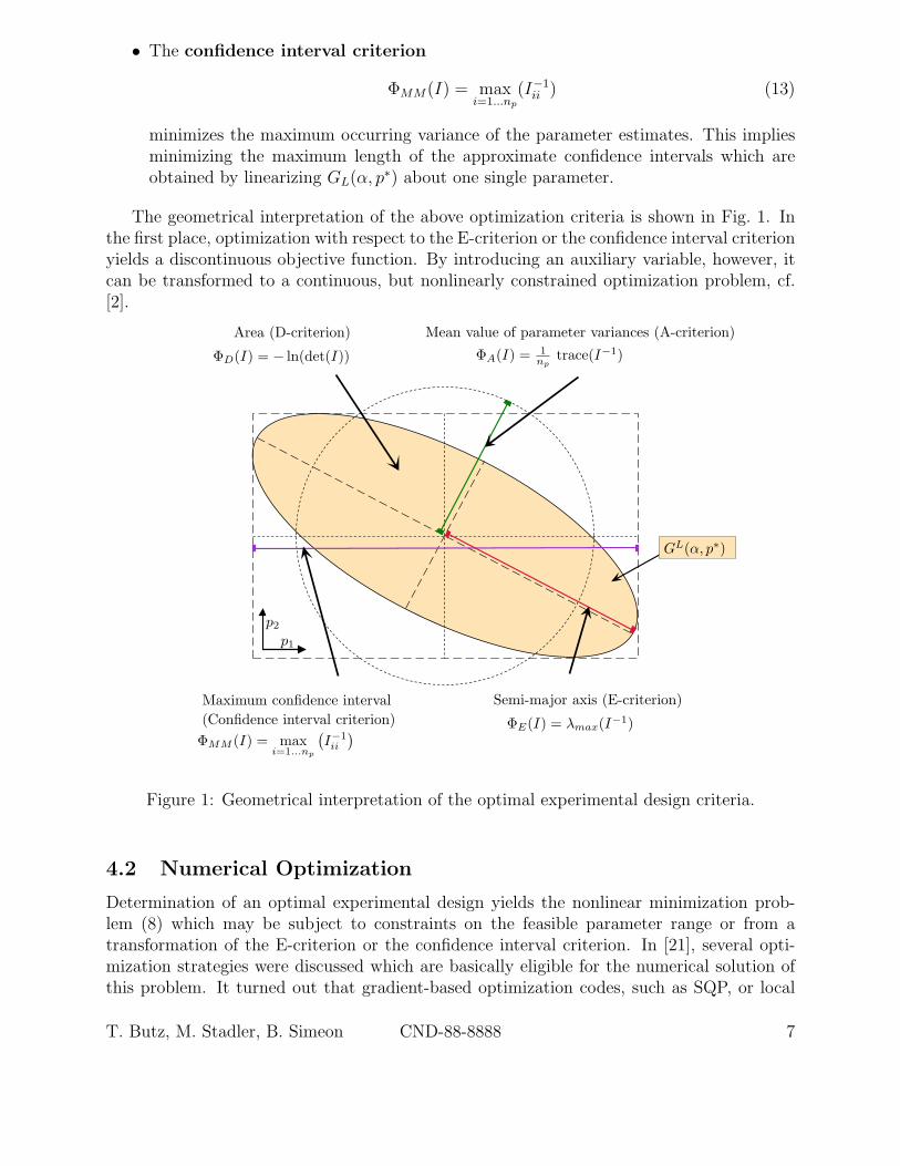
• The confidence interval criterion

ΦMM(I) = maxi=1...np

(I−1ii ) (13)

minimizes the maximum occurring variance of the parameter estimates. This impliesminimizing the maximum length of the approximate confidence intervals which areobtained by linearizing GL(α, p∗) about one single parameter.

The geometrical interpretation of the above optimization criteria is shown in Fig. 1. Inthe first place, optimization with respect to the E-criterion or the confidence interval criterionyields a discontinuous objective function. By introducing an auxiliary variable, however, itcan be transformed to a continuous, but nonlinearly constrained optimization problem, cf.[2].

Area (D-criterion) Mean value of parameter variances (A-criterion)

Semi-major axis (E-criterion)Maximum confidence interval(Confidence interval criterion)

GL(α, p∗)

ΦD(I) = − ln(det(I)) ΦA(I) = 1np

trace(I−1)

ΦE(I) = λmax(I−1)ΦMM (I) = max

i=1...np

(I−1ii

)

p1

p2

Figure 1: Geometrical interpretation of the optimal experimental design criteria.

4.2 Numerical Optimization

Determination of an optimal experimental design yields the nonlinear minimization prob-lem (8) which may be subject to constraints on the feasible parameter range or from atransformation of the E-criterion or the confidence interval criterion. In [21], several opti-mization strategies were discussed which are basically eligible for the numerical solution ofthis problem. It turned out that gradient-based optimization codes, such as SQP, or local


search strategies, e.g. pattern or exploratory search, are not practicable, when using thevehicle dynamics model in DYNA4 as simulation kernel. Instead, more robust algorithmsare required which are designed to avoid local minima and can cope with low smoothnessprerequisites. Therefore, we focus here on a quasi-Newton method for the solution of noisyoptimization problems and a global search strategy based on the design and analysis ofcomputer experiments (DACE).

The implicit filtering approach [13] is intended for the solution of noisy optimization prob-lems where a smooth objective function is superimposed by high-frequency low-amplitudedisturbances or even discontinuities. The underlying method is a projected quasi-Newtonalgorithm where the descent direction is determined from

H(k) s = −∇Φ(v(k)) . (14)

To avoid the computation of the Hesse matrix ∇2Φ(v(k)) an approximation H(k) is determinedby BFGS or symmetric rank one update. The length of the optimization step is obtainedfrom a line search. The required gradient information is provided by numerical differentiationusing one-sided or centered finite differences. Starting from a rather large value, the finitedifference increment is successively reduced, until no further progress is achieved in theoptimization. This strategy intends to first follow the rough structure of the objectivefunction, before increasing the resolution to a detailed search by use of small finite differencesteps in the proximity of the solution. In this way, the problem of prematurely terminatingwith a local minimum of the noisy function shall be avoided. For the numerical optimization,the implementation IFFCO by Kelley was used [6].

The second strategy is optimization by iteratively updated surrogate functions adoptedfrom the design and analysis of computer experiments for extremely expensive simulationmodels, such as finite elements. The underlying idea is to carry out the optimization with anapproximate model of the objective function which can be evaluated with low computationalcost. The value of the true objective function is only computed at the minimum of thesurrogate model and is used to successively refine the approximation. Though, a large partof the computational effort arises from the function evaluations required to obtain an initialapproximation.

The surrogate optimization method by Hemker [12] is based on a kriging model which isconstructed from the Matlab Toolbox DACE [17]. The surrogate model

Φ(v) = βT ξ(v) + Z(v) (15)

consists of a polynomial interpolation βT ξ(v) for the global trend of the objective functionwhich is superimposed by a stochastic process Z(v). The latter is a realization of a stationaryGaussian function with expectation 0 and a covariance matrix which depends on the varianceσ2 and the Gaussian correlation matrix R of the supporting points. The parameters of Z(v)and the polynomial coefficients β are determined by a maximum likelihood estimation. Thesurrogate model interpolates the original objective function at the supporting points exactlyand yields an infinitely differentiable optimization criterion over the entire feasible parameterregion. For a more detailed description of the construction and the update of the surrogatemodel we refer to [12, 20, 21]. The optimization is accomplished with the SQP code SNOPTby Gill [9].


0

5

10

15

0100

200300

400

−140

−120

−100

−80

−60

−40

−20

Frequency [Hz]Phase [deg]

D−

crite

rion

0

5

10

15

0100

200300

400

−140

−120

−100

−80

−60

−40


D−

crite

rion

0

5

10

15

0100

200300

400

−140

−120

−100

−80

−60

−40


D−

crite

rion

(a) after 1 iteration (b) after 5 iterations (c) after 10 iterations

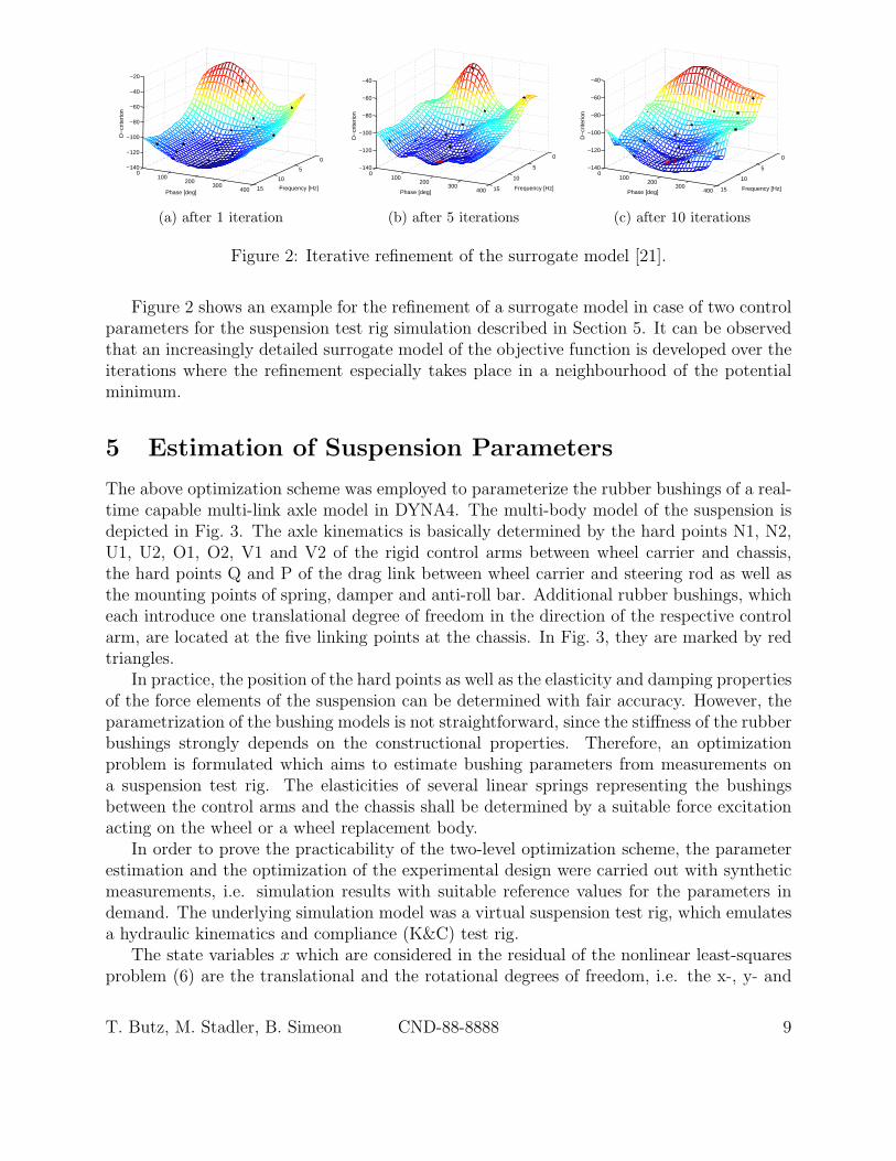
Figure 2: Iterative refinement of the surrogate model [21].

Figure 2 shows an example for the refinement of a surrogate model in case of two controlparameters for the suspension test rig simulation described in Section 5. It can be observedthat an increasingly detailed surrogate model of the objective function is developed over theiterations where the refinement especially takes place in a neighbourhood of the potentialminimum.

5 Estimation of Suspension Parameters

The above optimization scheme was employed to parameterize the rubber bushings of a real-time capable multi-link axle model in DYNA4. The multi-body model of the suspension isdepicted in Fig. 3. The axle kinematics is basically determined by the hard points N1, N2,U1, U2, O1, O2, V1 and V2 of the rigid control arms between wheel carrier and chassis,the hard points Q and P of the drag link between wheel carrier and steering rod as well asthe mounting points of spring, damper and anti-roll bar. Additional rubber bushings, whicheach introduce one translational degree of freedom in the direction of the respective controlarm, are located at the five linking points at the chassis. In Fig. 3, they are marked by redtriangles.

In practice, the position of the hard points as well as the elasticity and damping propertiesof the force elements of the suspension can be determined with fair accuracy. However, theparametrization of the bushing models is not straightforward, since the stiffness of the rubberbushings strongly depends on the constructional properties. Therefore, an optimizationproblem is formulated which aims to estimate bushing parameters from measurements ona suspension test rig. The elasticities of several linear springs representing the bushingsbetween the control arms and the chassis shall be determined by a suitable force excitationacting on the wheel or a wheel replacement body.

In order to prove the practicability of the two-level optimization scheme, the parameterestimation and the optimization of the experimental design were carried out with syntheticmeasurements, i.e. simulation results with suitable reference values for the parameters indemand. The underlying simulation model was a virtual suspension test rig, which emulatesa hydraulic kinematics and compliance (K&C) test rig.

The state variables x which are considered in the residual of the nonlinear least-squaresproblem (6) are the translational and the rotational degrees of freedom, i.e. the x-, y- and


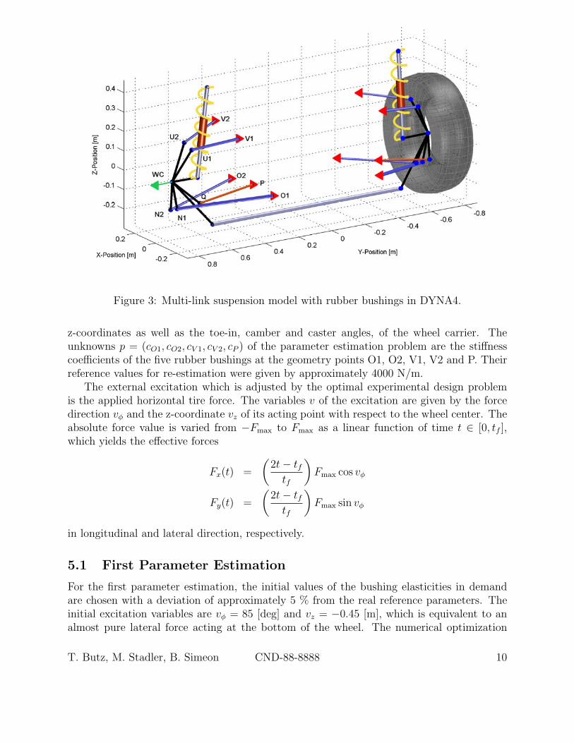
Figure 3: Multi-link suspension model with rubber bushings in DYNA4.

z-coordinates as well as the toe-in, camber and caster angles, of the wheel carrier. Theunknowns p = (cO1, cO2, cV 1, cV 2, cP ) of the parameter estimation problem are the stiffnesscoefficients of the five rubber bushings at the geometry points O1, O2, V1, V2 and P. Theirreference values for re-estimation were given by approximately 4000 N/m.

The external excitation which is adjusted by the optimal experimental design problemis the applied horizontal tire force. The variables v of the excitation are given by the forcedirection vφ and the z-coordinate vz of its acting point with respect to the wheel center. Theabsolute force value is varied from −Fmax to Fmax as a linear function of time t ∈ [0, tf ],which yields the effective forces

Fx(t) =

(2t − tf

tf

)Fmax cos vφ

Fy(t) =

(2t − tf

tf

)Fmax sin vφ

in longitudinal and lateral direction, respectively.

5.1 First Parameter Estimation

For the first parameter estimation, the initial values of the bushing elasticities in demandare chosen with a deviation of approximately 5 % from the real reference parameters. Theinitial excitation variables are vφ = 85 [deg] and vz = −0.45 [m], which is equivalent to analmost pure lateral force acting at the bottom of the wheel. The numerical optimization


with the Levenberg-Marquardt algorithm yields a small least-squares residual and very goodagreement with the reference data for the position and the orientation of the wheel carrier.In addition, very good estimates of the stiffness coefficients are already obtained which differless than 0.1 % from the original values [21].

−0.5 0 0.5 1 1.5

c_O1

c_O2

c_V1

c_V2

c_P

Par

amet

ers

log10

(diag(JTJ)−1)

Parameter Sensitivities

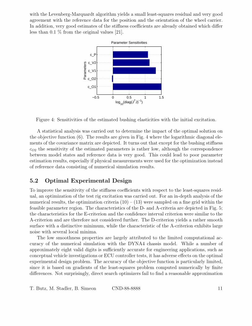
Figure 4: Sensitivities of the estimated bushing elasticities with the initial excitation.

A statistical analysis was carried out to determine the impact of the optimal solution onthe objective function (6). The results are given in Fig. 4 where the logarithmic diagonal ele-ments of the covariance matrix are depicted. It turns out that except for the bushing stiffnesscO2 the sensitivity of the estimated parameters is rather low, although the correspondencebetween model states and reference data is very good. This could lead to poor parameterestimation results, especially if physical measurements were used for the optimization insteadof reference data consisting of numerical simulation results.

5.2 Optimal Experimental Design

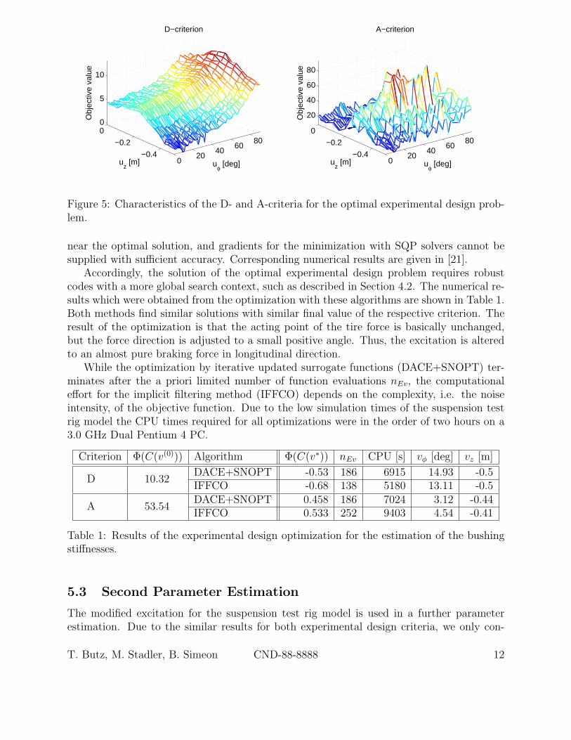
To improve the sensitivity of the stiffness coefficients with respect to the least-squares resid-ual, an optimization of the test rig excitation was carried out. For an in-depth analysis of thenumerical results, the optimization criteria (10) – (13) were sampled on a fine grid within thefeasible parameter region. The characteristics of the D- and A-criteria are depicted in Fig. 5;the characteristics for the E-criterion and the confidence interval criterion were similar to theA-criterion and are therefore not considered further. The D-criterion yields a rather smoothsurface with a distinctive minimum, while the characteristic of the A-criterion exhibits largenoise with several local minima.

The low smoothness properties are largely attributed to the limited computational ac-curacy of the numerical simulation with the DYNA4 chassis model. While a number ofapproximately eight valid digits is sufficiently accurate for engineering applications, such asconceptual vehicle investigations or ECU controller tests, it has adverse effects on the optimalexperimental design problem. The accuracy of the objective function is particularly limited,since it is based on gradients of the least-squares problem computed numerically by finitedifferences. Not surprisingly, direct search optimizers fail to find a reasonable approximation


020

4060

80

−0.4

−0.2

00

5

10

uφ [deg]

D−criterion

uz [m]

Obj

ectiv

e va

lue

020

4060

80

−0.4

−0.2

0

20

40

60

80

uφ [deg]

A−criterion

uz [m]

Obj

ectiv

e va

lue

Figure 5: Characteristics of the D- and A-criteria for the optimal experimental design prob-lem.

near the optimal solution, and gradients for the minimization with SQP solvers cannot besupplied with sufficient accuracy. Corresponding numerical results are given in [21].

Accordingly, the solution of the optimal experimental design problem requires robustcodes with a more global search context, such as described in Section 4.2. The numerical re-sults which were obtained from the optimization with these algorithms are shown in Table 1.Both methods find similar solutions with similar final value of the respective criterion. Theresult of the optimization is that the acting point of the tire force is basically unchanged,but the force direction is adjusted to a small positive angle. Thus, the excitation is alteredto an almost pure braking force in longitudinal direction.

While the optimization by iterative updated surrogate functions (DACE+SNOPT) ter-minates after the a priori limited number of function evaluations nEv, the computationaleffort for the implicit filtering method (IFFCO) depends on the complexity, i.e. the noiseintensity, of the objective function. Due to the low simulation times of the suspension testrig model the CPU times required for all optimizations were in the order of two hours on a3.0 GHz Dual Pentium 4 PC.

Criterion Φ(C(v(0))) Algorithm Φ(C(v∗)) nEv CPU [s] vφ [deg] vz [m]

D 10.32DACE+SNOPT -0.53 186 6915 14.93 -0.5IFFCO -0.68 138 5180 13.11 -0.5

A 53.54DACE+SNOPT 0.458 186 7024 3.12 -0.44IFFCO 0.533 252 9403 4.54 -0.41

Table 1: Results of the experimental design optimization for the estimation of the bushingstiffnesses.

5.3 Second Parameter Estimation

The modified excitation for the suspension test rig model is used in a further parameterestimation. Due to the similar results for both experimental design criteria, we only con-


sider the optimal solution for the D-criterion. Compared to the first estimation, the secondparameter optimization yields an even improved accuracy of the estimates. Since syntheticreference data was used, the stiffness coefficients for the bushing models can be re-identifiedup to computational accuracy.

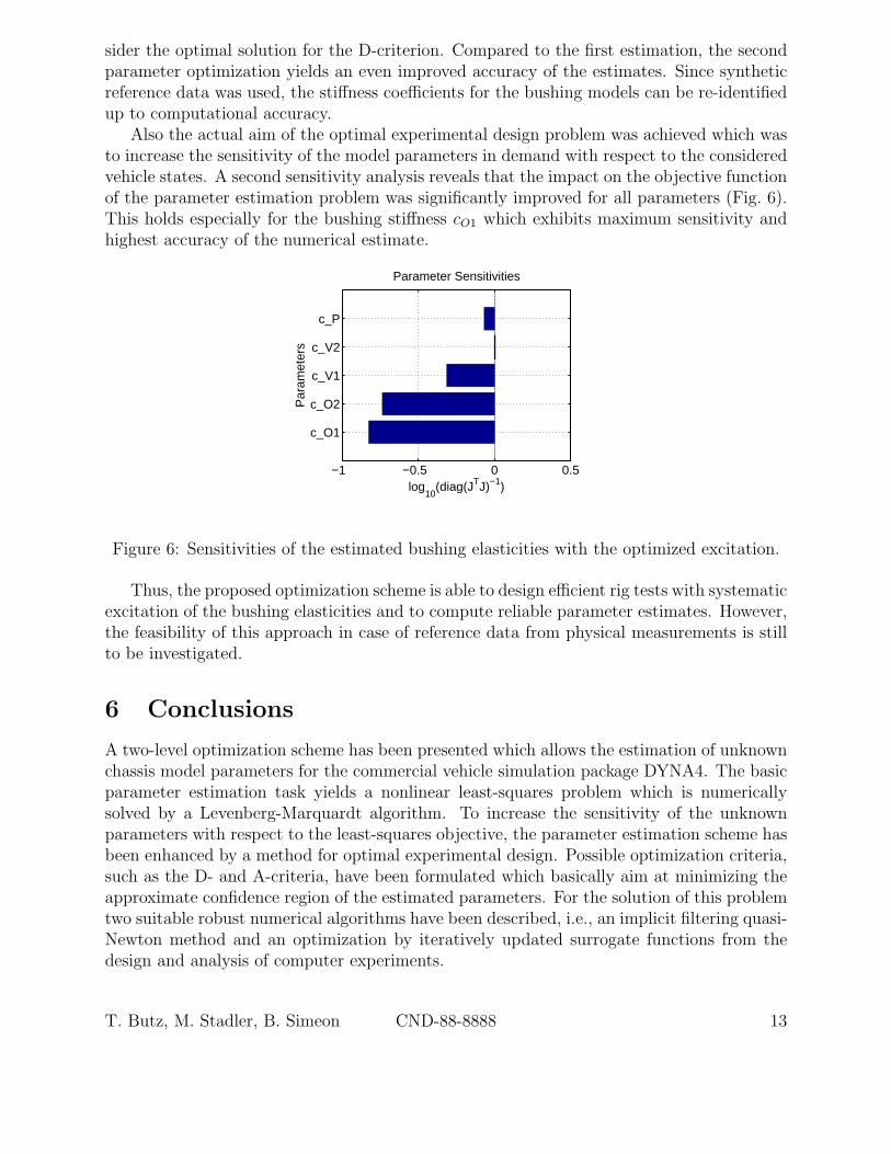
Also the actual aim of the optimal experimental design problem was achieved which wasto increase the sensitivity of the model parameters in demand with respect to the consideredvehicle states. A second sensitivity analysis reveals that the impact on the objective functionof the parameter estimation problem was significantly improved for all parameters (Fig. 6).This holds especially for the bushing stiffness cO1 which exhibits maximum sensitivity andhighest accuracy of the numerical estimate.

−1 −0.5 0 0.5

c_O1

c_O2

c_V1

c_V2

c_P

Par

amet

ers

log10

(diag(JTJ)−1)

Parameter Sensitivities

Figure 6: Sensitivities of the estimated bushing elasticities with the optimized excitation.

Thus, the proposed optimization scheme is able to design efficient rig tests with systematicexcitation of the bushing elasticities and to compute reliable parameter estimates. However,the feasibility of this approach in case of reference data from physical measurements is stillto be investigated.

6 Conclusions

A two-level optimization scheme has been presented which allows the estimation of unknownchassis model parameters for the commercial vehicle simulation package DYNA4. The basicparameter estimation task yields a nonlinear least-squares problem which is numericallysolved by a Levenberg-Marquardt algorithm. To increase the sensitivity of the unknownparameters with respect to the least-squares objective, the parameter estimation scheme hasbeen enhanced by a method for optimal experimental design. Possible optimization criteria,such as the D- and A-criteria, have been formulated which basically aim at minimizing theapproximate confidence region of the estimated parameters. For the solution of this problemtwo suitable robust numerical algorithms have been described, i.e., an implicit filtering quasi-Newton method and an optimization by iteratively updated surrogate functions from thedesign and analysis of computer experiments.


Numerical results have been reported for a sample application, the estimation of bush-ing stiffnesses for a real-time capable multi-body suspension model. Based on syntheticreference data from simulation results, it is possible to re-identify the unknown parametersaccurately. Optimizing the excitation for the underlying virtual suspension test rig furtherimproves the sensitivity of the parameters in demand and thus allows to find more reliableand even more accurate estimates. However, for the optimal experimental design problem,the low smoothness prerequisites of the objective function turned out to be problematic forcommon optimization codes. The successful minimization is mainly attributed to the use ofoptimization codes that are appropriate for very noisy problems.

Overall, this investigation shows that the parameter estimation results can be improvedby excitation strategies that are determined by solving the optimal experimental designproblem. Although the latter improvement had no considerable effect on the accuracy of theparameter estimation results in the case of synthetic reference data, well-conditioned opti-mization problems are especially important in the presence of measurement errors, e.g., whenusing physical measurements. Moreover, the measuring effort at test rigs or in field tests maybe reduced by carrying out experiments with systematically optimized control variables andexternal excitations. The feasibility of our approach for more complex parameter estimationproblems and in the presence of physical measurements is still to be investigated.

References

[1] I. Bauer, H. G. Bock, S. Korkel, J. P. Schloder. Numerical methods for optimum exper-imental design in DAE systems. Journal of Computational and Applied Mathematics120, 2000, 1-25.

[2] E. Biber. Identifikation der Lastparameter von Industrierobotern. Diploma Thesis, Zen-trum Mathematik, Technische Universitat Munchen, 2000.

[3] T. Butz, O. von Stryk, C. Chucholowski, S. Truskawa, T.-M. Wolter: Modeling Tech-niques and Parameter Estimation for the Simulation of Complex Vehicle Structures. In:M. Breuer, F. Durst, C. Zenger (eds.): High-Performance Scientific and EngineeringComputing. Lecture Notes in Computational Science and Engineering 21, Springer-Verlag, 2002, 333-340.

[4] P. Eberhard, U. Piram, D. Bestle: Optimization of Damping Characteristics in VehicleDynamics. Engineering Optimization 31, 1999, 435-455.

[5] B. Esterl, T. Butz, B. Simeon, B. Burgermeister. Real-time integration and vehicletrailer-coupling by algorithms for differential-algebraic equations. Vehicle System Dy-namics 45 (9), 2007, 819-834.

[6] T. D. Choi, O. J. Eslinger, P. A. Gilmore, C. T. Kelley, H. A. Patrick. Users Guideto IFFCO. Technical Report, Center for Research in Scientific Computation, NorthCarolina State University, 2001.

[7] J. Dongarra, E. Grosse. Netlib Repository. http://www.netlib.org, 2006.


[8] M. Gilg. Parameteridentifizierung und -optimierung am Beispiel einer Hinterachskine-matik. Diploma Thesis, Zentrum Mathematik, Technische Universitat Munchen, 2004.

[9] P. E. Gill, W. Murray, M. A. Saunders. User’s Guide for SNOPT 5.3: A FortranPackage for Large-Scale Nonlinear Programming. Technical Report SOL 97-3, StanfordUniversity, 1997.

[10] P. E. Gill, W. Murray, M. A. Saunders, M. H. Wright: Some Theoretical Propertiesof an Augmented Lagrangian Merit Function. In: P. M. Pardalos (Ed.): Advances inOptimization and Parallel Computing, North Holland, 1992, 101-128.

[11] P. E. Gill, W. Murray, M. A. Saunders, M. H. Wright: User’s Guide for NPSOL 5.0: AFortran Package for Nonlinear Programming. Technical Report NA 98-2, Departmentof Mathematics, University of California, San Diego, 1998.

[12] T. Hemker, K. R. Fowler, O. von Stryk. Derivative-Free Optimization Methods for Han-dling Fixed Costs in Optimal Groundwater Remediation Design. In: P. J. Binning, P. K.Engesgaard, H. K. Dahle, G. F. Pinder and W. G. Gray: Proceedings of the XVI In-ternational Conference on Computational Methods in Water Resources, Copenhagen,19-22 June 2006.

[13] C. T. Kelley. Iterative Methods for Optimization. Frontiers in Applied Mathematics 18,SIAM, 1999.

[14] S. Korkel. Numerische Methoden fur Optimale Versuchsplanungsprobleme bei nichtlin-earen DAE-Modellen. PhD Thesis, Interdisziplinares Zentrum fur WissenschaftlichesRechnen, Universitat Heidelberg, 2002.

[15] T. W. Lohmann, H. G. Bock. A Computationally Convenient Statistical Analysis ofthe Solution of Constrained Least-Squares Problems. Technical Report, Zentrum Math-ematik, Technische Universitat Munchen, 1996.

[16] J. J. More. The Levenberg-Marquardt Algorithm: Implementation and Theory. In: A.Dold, B. Eckmann (eds.). Numerical Analysis. Lecture Notes in Mathematics 630,Springer, Berlin Heidelberg, 1978, 105-116.

[17] H. B. Nielsen. DACE. http://www2.imm.dtu.dk/ hbn/dace/, 2006.

[18] F. Pukelsheim. Optimal Design of Experiments. John Wiley & Sons, Inc., New York,1993.

[19] Rill, G., Simulation von Kraftfahrzeugen, Vieweg, Braunschweig, 1994.

[20] M. J. Sasena. Flexibility and Efficiency Enhancements for Constrained Global DesignOptimization with Kriging Approximations. PhD Thesis, University of Michigan, 2002.

[21] M. Stadler. Optimale Versuchsplanung zur Identifizierung von Fahrzeugparametern.Diploma Thesis, Zentrum Mathematik, Technische Universitat Munchen, 2006.


[22] TESIS DYNAware. DYNA4 User Manual. Munchen, 2008.

[23] W. J. Welch, R. J. Buck, J. Sacks, H. P. Wynn, T. J. Mitchell, M. D. Morris. Screening,Predicting, and Computer Experiments. Technometrics 34, 1, 1992, 15-25.


Documents

Butz Simeon Stadler Jc Nd