Embed Size (px)
Citation preview
Policy Research Working Paper 8104
But …What Is The Poverty Rate Today?
Testing Poverty Nowcasting Methods in Latin America and the Caribbean
German CarusoLeonardo LucchettiEduardo Malasquez
Thiago ScotR. Andrés Castañeda
Poverty and Equity Global Practice GroupJune 2017
WPS8104P
ublic
Dis
clos
ure
Aut
horiz
edP
ublic
Dis
clos
ure
Aut
horiz
edP
ublic
Dis
clos
ure
Aut
horiz
edP
ublic
Dis
clos
ure
Aut
horiz
ed
Produced by the Research Support Team
Abstract
The Policy Research Working Paper Series disseminates the findings of work in progress to encourage the exchange of ideas about development issues. An objective of the series is to get the findings out quickly, even if the presentations are less than fully polished. The papers carry the names of the authors and should be cited accordingly. The findings, interpretations, and conclusions expressed in this paper are entirely those of the authors. They do not necessarily represent the views of the International Bank for Reconstruction and Development/World Bank and its affiliated organizations, or those of the Executive Directors of the World Bank or the governments they represent.
Policy Research Working Paper 8104
This paper is a product of the Poverty and Equity Global Practice Group. It is part of a larger effort by the World Bank to provide open access to its research and make a contribution to development policy discussions around the world. Policy Research Working Papers are also posted on the Web at http://econ.worldbank.org. The authors may be contacted at [email protected].
Poverty estimates usually lag behind two years, which makes it difficult to provide real-time poverty analysis to assess the impact of economic crisis and shocks among the less well-off, and subsequently limits policy responses. This paper takes advantage of up-to-date average economic welfare indicators like the gross domestic product per capita and comprehen-sive harmonized micro data of more than 180 household surveys in 15 Latin American countries. The paper tests three commonly used poverty nowcasting methods and
ranks their performance by comparing country-specific and regional poverty nowcasts with actual poverty estimates for 2003–14 period. The validation results show that the two bottom-up approaches, which simulate the performance of each agent in the economy to nowcast overall poverty, perform relatively better than the top-down approach, which uses welfare estimates to explain the performance of poverty at an aggregate level over time. The results are robust to additional sensitivity and robustness tests.
But… What Is The Poverty Rate Today?
Testing Poverty Nowcasting Methods in Latin America and the Caribbean
German Caruso Leonardo Lucchetti§
Eduardo Malasquez† Thiago Scot‡
R. Andrés Castañeda††
JEL classification: D31, I3, I31, D6
Key words: Poverty, Nowcasting, Latin America and the Caribbean, Validation
We are grateful to Oscar Calvo-Gonzalez, Samuel Jaime Pienknagura, German Reyes, Liliana Sousa, Daniel
Valderrama, Carlos Vegh, and Nobuo Yoshida whose suggestions greatly improved earlier drafts of the paper. All
remaining errors are ours. World Bank. E-mail: [email protected] § World Bank. E-mail: [email protected]† World Bank. E-mail: [email protected]‡ University of California at Berkeley. E-mail: [email protected]†† World Bank. E-mail: [email protected]
2
1 Introduction
Among all the socioeconomic indicators developed during the last two centuries, the share of the
population living in poverty has become one of the most studied and monitored (Ravallion 2016,
chap. 1). A good poverty measurement and profiling identifies the poor and targets and monitors
all interventions designed to benefit the most disadvantaged groups in society. Thus, there is an
increasing interest from academics and policy makers to know the current poverty status at the
country, regional, and global levels to design policy solutions that alleviate the situation of the less
well-off.1 Nonetheless, due to data collection and processing time, poverty indicators are generally
released with one or more years of lag. This delay makes it challenging to provide real-time
poverty analysis and to strengthen the dialogue on the implementation of policies to mitigate the
poverty impact of shocks like economic crisis or natural disasters.2
Departing from the basic intuition that the performance of poverty depends on the evolution
of national welfare aggregates like the GDP per capita, it is expected that poverty forecasting relies
on the accuracy of forecasted GDP. That is, if the forecasted GDP were off, the forecasted poverty
would be off as well. However, the main difference between nowcasting and forecasting poverty
is that the GDP per capita is actual for the former, while it is forecasted for the latter. By validating
three poverty forecasting methods with actual GDP information, this paper bridges the gap of
knowledge between the most recent poverty numbers available and the current calendar year.
Additionally, it provides empirical evidence for the reliability of such methods to enlighten the
current situation of poverty, rather than its performance in the future.
Generally speaking, poverty forecasting provides a series of possible, future GDP scenarios
whose poverty outcomes are determined by the poverty forecasting method. That is, poverty
forecasting is an attempt to understand the performance of poverty if the GDP scenario
assumptions are met and the poverty forecasting method is accurate (Karver, Kenny, and Sumner
1 For instance, extreme poverty reduction was among the most important indicators in the Millennium Development
Goals (MDGs), while the World Bank recently adopted the goal of ending extreme poverty at the global level by 2030.
The World Bank measures global overall poverty as life under a US$1.9 per person per day in 2011 Purchasing Power
Parity (PPP) (Ferreira et al. 2016, Dean and Prydz 2015). Similarly, the World Bank estimates the regional overall
poverty in the LAC region as having an income below the US$4 per person per day poverty line in 2005 PPPs
(Gasparini et al. 2013, Castaneda et al. 2016). 2 For instance, the latest global poverty estimates produced by the World Bank are from 2013, while the most recent
Latin American and the Caribbean regional estimates are from 2014 (see Castaneda et al. 2016 for the 2014 LAC
regional estimates).
3
2012; Ravallion 2012; Ravallion 2013; Edward and Sumner 2013; Chandy, Ledlie, and
Penciakova 2013; Yoshida, Uematsu, and Sobrado 2014; and Poverty Research Report, The World
Bank 2000). In contrast, given that poverty nowcasting relies on actual GDP data, its accuracy
depends only on the features of each nowcasting method.
The purpose of this paper is to provide a comprehensive analysis of several methods for
poverty nowcasting to get real-time poverty estimates in Latin America and the Caribbean (LAC).
To this end, the paper first documents existing methodologies for poverty nowcasting by
describing in detail their main assumptions, their information requirements, and their main
limitations. Then, it validates the performance of these methods by comparing nowcasted poverty
numbers with actual poverty estimates. In the particular case of the LAC region, National
Statistical Offices (NSOs) usually release poverty numbers with one year of lag. Thus, this paper
validates these poverty nowcasting methods one year ahead.
Three contributions to the literature on poverty nowcasting—and forecasting—stem from
this paper. First, this paper develops a methodological framework to understand the errors of these
techniques for poverty nowcasting. Second, this analysis validates the methods using a set of about
180 harmonized micro household datasets available for 15 countries in LAC for the 2003–14
period. By using this comprehensive database, the paper minimizes the possibility of arriving to
conclusions based on biased samples of countries or spurious results. Finally, the paper assesses
the robustness of the results and quantifies the accuracy of each method by empirically testing the
magnitude of the errors in each methodology.
Our results suggest that the three methods are promising for nowcasting both large poverty
reductions as well as poverty stagnation in the region one year ahead. In general, the two bottom-
up approaches that simulate the performance of each agent in the economy to nowcast poverty
perform better than the top-down approach that uses welfare estimates to explain the performance
of poverty at an aggregate level over time. The paper also provides evidence that the results are in
general stable to changes in the underlying parameters used for producing poverty nowcasts.
The paper is organized as follows. Section 2 introduces the three approaches for
nowcasting poverty and the theoretical framework of the nowcasting errors. Section 3 presents the
data used and the empirical approach. Section 4 presents the validation results of the poverty
nowcasting in LAC. Section 5 shows the stress and sensitivity analysis of the methods. Finally,
section 6 concludes.
4
2 Poverty forecasting methods in practice
The projection of poverty headcount is nothing else than “non-linear functions of underlying
changes in average income and measures of income inequality” (Kraay 2006, 200). That is, the
analysis of the performance of certain covariates that are assumed to have a significant and known
effect on the welfare distribution, so that we are able to estimate the new share of population under
a particular welfare threshold in a subsequent period for which there are no microdata available.
The literature presents several methods to identify the main determinants and forecast poverty,
though little is known about their level of accuracy and performance. These methods vary in terms
of their assumptions and level of sophistication, which can be framed under two general
approaches: “top-down” and “bottom-up” methods.
2.1 Top-down approaches
These approaches use economic indicators like Gross Domestic Product (GDP) growth to explain
the performance of poverty at an aggregate level over time. One of the top-down approaches most
widely used is the Poverty-growth Elasticity (PE hereafter) method. The simplest version of this
method consist of the ratio between the percent change in the poverty headcount and the percent
change of a welfare aggregate measure –e.g., GDP per capita- in two moments in time, that is
𝐸𝑡,𝑡−1 =
Δ𝑃𝑡/𝑃𝑡−1
Δ𝑌𝑡/𝑌𝑡−1
(1)
where Δ𝑃𝑡 = 𝑃𝑡 − 𝑃𝑡−1 is the change in the poverty headcount and Δ𝑌𝑡 = 𝑌𝑡 − 𝑌𝑡−1 is the change
in the aggregate measure of welfare. Assuming that the elasticity 𝐸𝑡,𝑡−1 has a unique non-stochastic
value over time for any poverty measure, poverty in period 𝑡 + 1 can be projected as follows
𝑃𝑡+1 ≈ 𝑃𝑡(1 +
Δ𝑌𝑡
𝑌𝑡−1𝐸𝑡,𝑡−1) (2)
Elasticities have proved to perform well for poverty forecasting in cross-country settings
(Bourguignon 2003, Klasen and Misselhorn 2006, and Yoshida et al. 2014). However, it can be
shown that the relationship between growth and poverty tends to decrease when poverty decreases
and therefore they may not work properly when forecasting poverty rates in long periods of time
(Yoshida et al. 2014).
5
Kakwani (1993) proposes a methodology that assumes that the Lorenz curve shifts entirely
by an offset factor,3 which leads to a rigid structure of inequality but provides a useful
simplification. With these in hand, the author calculates elasticities of poverty with respect to both
changes in mean income and Gini coefficient. Results show that, for the case of Côte d’Ivoire, the
measures of poverty are highly elastic to changes in income inequality and mean income, with the
income elasticity being considerably higher. Dollar and Kraay (2002) and Kraay (2006) find
different results for a large set of countries where the average income growth is the main and most
important driver of poverty reduction. Similarly, Datt and Ravallion (1992) decomposes changes
in poverty in Brazil and India in the 1980s, finding that the effect of growth on poverty
overshadows the redistribution effect for most of the pairs of years studied. This implies that,
depending on the country and its current characteristics, poverty might be determined either by the
growth of the economy or by the distribution of welfare in a particular period.
By adding temporality to the analysis, Ravallion and Chen (1997, 360) suggest a simple
model in which the Lorenz curve may change from one period to another. In this case, the elasticity
can take any sign or magnitude and it has its own distribution, that is
Log 𝑃𝑡 = 𝛼 + B logY𝑡 + 𝛾𝑡 + 𝜖𝑡 (3)
where B is an empirical growth elasticity, 𝛼 is a time-persistent effect, and 𝛾 is a time trend. Given
that it is impossible to observe the true mean of the GDP or consumption per capita 𝑌𝑡∗, the
regressions must be done with what is actually observed, 𝑌𝑡.
More sophisticated models attempt to incorporate other aggregate variables like inequality,
but given that several combinations of two or more aggregate variables may produce the same
poverty forecast, the exercise must be done by assessing the plausibility of different scenarios
(Ravallion 2012; Ravallion 2013).
2.2 Bottom-up approaches
These approaches simulate the performance—or even the behavior—of each agent in the economy
to generate a new welfare aggregate used to estimate poverty. The most basic model assumes that
all households’ incomes are re-scaled by the same factor, say GDP per capita growth (Yoshida et
al. 2014). This method, known as Neutral Distribution Growth (NDG hereafter), usually performs
3 Namely, 𝐿∗(𝑝) = 𝐿(𝑝) − 𝜆[𝑝 − 𝐿(𝑝)], where 𝐿 is the original Lorenz curve, 𝐿∗ is the shifted one, and 𝜆 is the
percentage change of the Gini coefficient.
6
well as long as inequality remains stable. Karver, Kenny, and Sumner (2012) explain that poverty
forecast based on past trends is a naïve approach to forecasting due to the high volatility of poverty.
Instead, they select three different scenarios based on IMF growth projections and predict poverty
rates for all countries, assuming static inequality in a 20-year period. As explained by the authors,
the assumption of a neutral distribution is strong and it may bias the results in exercises that involve
long-run predictions like theirs. In this paper, in contrast, the validation of poverty estimates is
done from one year to another; a small period of time in which inequality changes are null or very
small, especially in LAC where income inequality has decreased considerably in the past decade
in most of the countries and then recently stagnated (Cord et al. 2017).
Complex models in which income distribution is not assumed stable provide deeper
understanding of the relation between specific segments of the economy and the evolution of
poverty rates. Olivieri et al. (2014) developed a technique and software module—ADePT
Simulation—to forecast the distribution of incomes by incorporating projections of other
aggregates such as economic output and employment by sector; prices; and population growth.
Other methods disaggregate the country’s population into proportionally-augmented bands of
welfare aggregates in order to relax the assumption of static distribution (Edward 2006; Edward
and Sumner 2013), or simply assume different inequality scenarios by shifting the proportion of
economic growth from the top 10 percent to the bottom 40 (Chandy, Ledlie, and Penciakova 2013).
The main advantage of the method is that it produces income forecasts at the household-level and
allows predicting distributional measures besides poverty. However, data requirements are
significant and therefore it is costly to apply the method to several countries at the same time and
in a consistent manner, which is one of the main objectives of this paper.
2.3 The approach of this paper
The two approaches most widely used today to nowcast poverty are the PE and the NDG methods.
Although simple to implement, the PE method has limited application because it produces only
aggregated -as opposed to household or individual level- poverty extrapolations. On the other
hand, unlike the PE method, the main advantage of the NDG method is that it produces income
estimates at the household-level. However, since all household incomes are multiplied by the same
economic growth rate, the method cannot be used for distributional analysis.
7
To overcome these limitations, we also analyze a generalized form of the NDG method, in
which different sections of the income distribution are assumed to grow at different rates,
following a specific and ad-hoc algorithm. This approach attempts to capture the heterogeneity of
growth across individuals or households by assuming that quantile-specific contributions to
growth during a known-data period remain similar during the unknown-data period. This
assumption is an extension of the “share of incremental income” definition of pro-poor growth
studied by White and Anderson (2001). The authors explain that if the share of total income growth
(𝑌𝑡 − 𝑌𝑡−1) that corresponds to the income growth of the poor (𝑌𝑡𝑃 − 𝑌𝑡−1
𝑃 ) from time 𝑡 − 1 to 𝑡 is
higher than from 𝑡 − 2 to 𝑡 − 1, the economy can be classified as pro-poor. Instead of studying
the contribution of the poor population, which varies over time, we analyze the contribution of
each quantile to total growth and assume stability over time. We refer to this method as Quantile
Growth Contribution (QGC).
Two main assumptions are required under QGC. First, the method assumes that people
with similar welfare aggregates in one period will perform similarly in the next period. That is, we
expect that, after ranking the population by quantiles based on welfare, two households within the
same quantile in period t will belong to the same quantile in period 𝑡 + 1. Second, the method
assumes that the economy performs today as it did in the past.
Data requirements needed to implement all these three methods are fairly reasonable and
therefore they can be applied in our setting: to nowcast poverty estimates in many countries and
years and in a consistent manner. In addition, all these methods have real-life applications and
have been extensively used to nowcast and forecast poverty estimates. For instance, the World
Bank uses the NDG method to extrapolate poverty estimates from the latest surveys available
(Yoshida et al. 2014), while it uses the PE method to produce poverty forecasts based on per capita
GDP forecasts (World Bank 2015; Yoshida et al. 2014).
3 Analytical assessment of measuring poverty in real time
3.1 Poverty measurement in the world and in LAC
Since the early 1990s, the World Bank has measured global poverty based on a comparable total
household per capita welfare measure and an international poverty line, both expressed in the same
purchasing power in all countries of the world (Ferreira et al. 2016). In the particular case of LAC,
income is the proxy for welfare most commonly used. Even when consumption is usually preferred
8
in the literature, income has been widely used in practice in the region since consumption is rarely
collected by the national statistical offices (NSOs) in LAC.
Due to the time required for household data collection and processing, household surveys
are usually available only with a two or more years lag. This makes it extremely challenging to
provide real-time poverty analysis. Although LAC is the region with most frequent household
surveys, the region is not an exception; the latest data available are from 2014 in most of the
countries in the region. To address this knowledge gap, this paper provides validations of three
alternative methods widely applied to nowcast poverty estimates both at the country as well as at
the regional level and provides up-to-date poverty estimates in the region.
Despite being outdated, poverty data in LAC are more up-to-date than most of other regions
in the world. In addition, the quality of the data is usually superior in many dimension. For
instance, surveys have in general more coverage –i.e., over 90 percent of LAC’s population is
covered by poverty data since the 1990s -- data are more frequent –i.e., about 60 percent of the
countries in LAC have more than three data points (Serajuddin et al. 2015)-, and surveys are
available for many years and usually comparable over time in most of the LAC countries. Having
several years of data offers at least two advantages. First, the years considered (2003-14) coincide
with a period of large poverty drops as well as poverty stagnation, which allows us to validate
methods under different scenarios of poverty changes. Second, having several years allows us to
test the robustness of some methods to the use of different past information. For all these reasons,
this paper focuses in the LAC region to validate existing poverty nowcasting methods.
3.2 Methods used for poverty nowcasting
This section presents the data environment and the three methods used to nowcast poverty
estimates. The analysis is performed in three periods of time: periods –2, –1, and 0; the first two
periods refer to the past when household surveys and national accounts information are available,
while period 0 refers to the present when only national accounts information is available. Notice
that the sequence in the nomenclature of the periods (i.e., –2, –1, and 0) does not imply that they
are adjacent or subsequent to each other; rather that the sequence is in a chronological order where
each period could be several years apart from the other. For the sake of simplicity we neglected
population growth in our estimations, as nowcasting generally implies very short periods of time
in which data availability is missing and for which population growth is usually negligible.
9
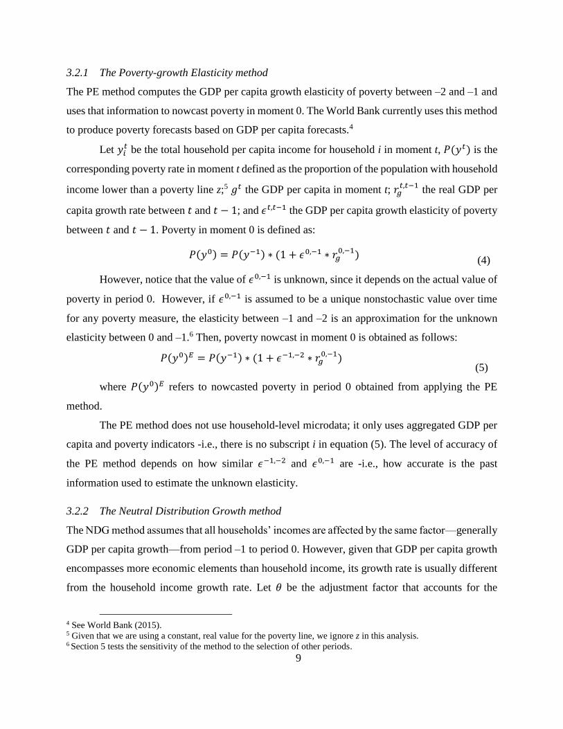
3.2.1 The Poverty-growth Elasticity method
The PE method computes the GDP per capita growth elasticity of poverty between –2 and –1 and
uses that information to nowcast poverty in moment 0. The World Bank currently uses this method
to produce poverty forecasts based on GDP per capita forecasts.4
Let 𝑦𝑖𝑡 be the total household per capita income for household i in moment t, 𝑃(𝑦𝑡) is the
corresponding poverty rate in moment t defined as the proportion of the population with household
income lower than a poverty line z;5 𝑔𝑡 the GDP per capita in moment t; 𝑟𝑔𝑡,𝑡−1
the real GDP per
capita growth rate between 𝑡 and 𝑡 − 1; and 𝜖𝑡,𝑡−1 the GDP per capita growth elasticity of poverty
between 𝑡 and 𝑡 − 1. Poverty in moment 0 is defined as:
𝑃(𝑦0) = 𝑃(𝑦−1) ∗ (1 + 𝜖0,−1 ∗ 𝑟𝑔0,−1)
(4)
However, notice that the value of 𝜖0,−1 is unknown, since it depends on the actual value of
poverty in period 0. However, if 𝜖0,−1 is assumed to be a unique nonstochastic value over time
for any poverty measure, the elasticity between –1 and –2 is an approximation for the unknown
elasticity between 0 and –1.6 Then, poverty nowcast in moment 0 is obtained as follows:
𝑃(𝑦0)𝐸 = 𝑃(𝑦−1) ∗ (1 + 𝜖−1,−2 ∗ 𝑟𝑔0,−1)
(5)
where 𝑃(𝑦0)𝐸 refers to nowcasted poverty in period 0 obtained from applying the PE
method.
The PE method does not use household-level microdata; it only uses aggregated GDP per
capita and poverty indicators -i.e., there is no subscript i in equation (5). The level of accuracy of
the PE method depends on how similar 𝜖−1,−2 and 𝜖0,−1 are -i.e., how accurate is the past
information used to estimate the unknown elasticity.
3.2.2 The Neutral Distribution Growth method
The NDG method assumes that all households’ incomes are affected by the same factor—generally
GDP per capita growth—from period –1 to period 0. However, given that GDP per capita growth
encompasses more economic elements than household income, its growth rate is usually different
from the household income growth rate. Let 𝜃 be the adjustment factor that accounts for the
4 See World Bank (2015). 5 Given that we are using a constant, real value for the poverty line, we ignore z in this analysis. 6 Section 5 tests the sensitivity of the method to the selection of other periods.
10
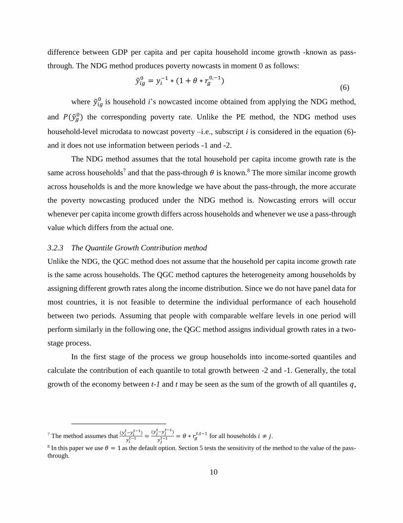
difference between GDP per capita and per capita household income growth -known as pass-
through. The NDG method produces poverty nowcasts in moment 0 as follows:
�̃�𝑖𝑔0 = 𝑦𝑖
−1 ∗ (1 + 𝜃 ∗ 𝑟𝑔0,−1)
(6)
where �̃�𝑖𝑔0 is household i’s nowcasted income obtained from applying the NDG method,
and 𝑃(�̃�𝑔0) the corresponding poverty rate. Unlike the PE method, the NDG method uses
household-level microdata to nowcast poverty –i.e., subscript i is considered in the equation (6)-
and it does not use information between periods -1 and -2.
The NDG method assumes that the total household per capita income growth rate is the
same across households7 and that the pass-through 𝜃 is known.8 The more similar income growth
across households is and the more knowledge we have about the pass-through, the more accurate
the poverty nowcasting produced under the NDG method is. Nowcasting errors will occur
whenever per capita income growth differs across households and whenever we use a pass-through
value which differs from the actual one.
3.2.3 The Quantile Growth Contribution method
Unlike the NDG, the QGC method does not assume that the household per capita income growth rate
is the same across households. The QGC method captures the heterogeneity among households by
assigning different growth rates along the income distribution. Since we do not have panel data for
most countries, it is not feasible to determine the individual performance of each household
between two periods. Assuming that people with comparable welfare levels in one period will
perform similarly in the following one, the QGC method assigns individual growth rates in a two-
stage process.
In the first stage of the process we group households into income-sorted quantiles and
calculate the contribution of each quantile to total growth between -2 and -1. Generally, the total
growth of the economy between t-1 and t may be seen as the sum of the growth of all quantiles 𝑞,
7 The method assumes that (𝑦𝑖
𝑡−𝑦𝑖𝑡−1)
𝑦𝑖𝑡−1 =
(𝑦𝑗𝑡−𝑦𝑗
𝑡−1)
𝑦𝑗𝑡−1 = 𝜃 ∗ 𝑟𝑔
𝑡,𝑡−1 for all households 𝑖 ≠ 𝑗.
8 In this paper we use 𝜃 = 1 as the default option. Section 5 tests the sensitivity of the method to the value of the pass-
through.
11
Δ𝑌𝑡,𝑡−1 = ∑(𝑟𝑞𝑡,𝑡−1 ∗ 𝑌𝑞
𝑡−1)
𝑄
𝑞=1
(7)
where 𝑌𝑡 = ∑ (𝑦𝑖𝑡)𝑖 is the total income of the economy, 𝑌𝑞
𝑡 is the total income of quantile q in
period t, and 𝑟𝑞𝑡,𝑡−1
is the growth rate of total income of quantile 𝑞 from period t to period t–1.9
We then assume that the contribution of each quantile to total growth in the unknown-data
period (i.e., -1 and 0) is the same as the contribution in the known-data period (i.e., -2 and -1), that
is
�̂�𝑞0 = 𝑆𝑞
−1,−2 ∗ Δ𝑌0,−1 + 𝑌𝑞−1
(8)
where �̂�𝑞0 is the nowcasted total income of quantile q in moment 0 and 𝑆𝑞
−1,−2 =Δ𝑌𝑞
−1,−2
Δ𝑌−1,−2 is the
contribution of quantile q to the total income growth between -1 and -2.
The second stage of the process is to distribute �̂�𝑞0 among households 𝑖 in quantile 𝑞. We
consider two different approaches. The first approach assumes a democratic scenario in which all
households within a quantile receive the same per-capita income amount.
�̂�𝑖𝑞
0 =�̂�𝑞
0
𝑛𝑞−1
(9)
where 𝑛𝑞−1 is the number of households in quantile 𝑞 in moment –1. This approach underlines the
assumption that households within the same quantile are similar. The second approach, a
plutocratic scenario, assumes that each household receives an amount of income based on its share
of the total income within its quantile in period -1.
�̂�𝑖𝑞
0 =𝑦𝑖𝑞
−1
𝑌𝑞−1
∗ �̂�𝑞0 (10)
Whereas the plutocratic approach considers relative differences between households within
the same quantile, the democratic approach is less intuitive but straightforward. In this paper, we
use the former. Replacing (8) in (10) and assuming no population growth, the characterization of
household i’s income under the QGC method is
9 Notice that if growth rates 𝑟𝑞
−1,−2 were the same rate r for all quantiles, we would be under the NDG scenario
(Δ𝑌−1,−2 = 𝑟−1,−2 ∗ 𝑌−2 = 𝜃 ∗ 𝑟𝑔−1,−2𝑌−2).
12
�̂�𝑖𝑞𝑔
0 =𝑦𝑖𝑞
−1
𝑌𝑞−1
∗ (𝑆𝑞−1,−2 ∗ 𝜃 ∗ 𝑟𝑔
0,−1 ∗ 𝑌−1 + 𝑌𝑞−1) (11)
This paper does not attempt to prove the goodness of fit of any of these methods. Each
method has its own assumptions and properties, which are validated under actual data scrutiny.
Notice that the QGC approach, in particular, is not an improvement of the NDG approach, but the
same methodology under different assumptions. The NDG assumes that all households—and
therefore quantiles—grow at the same pace, whereas QGC assumes that each quantile grows
according to its contribution to total growth in a known-data period.
3.3 Theoretical framework for nowcasting errors
As discussed in section 3.2, all methods need to make some assumptions in order to produce
poverty nowcasts in period 0 –i.e., knowledge of the elasticity, the pass-through, and the
contribution of every household to the change in total incomes. Therefore, errors will arise
whenever those assumptions are not met. This section presents the errors that arise from all these
assumptions.
3.3.1 Error under the PE method
The main assumption of the PE method is that the value of the elasticity between 0 and -1 is known.
However, that elasticity is unknown and needs to be estimated in reality. In this paper we use the
value of the elasticity between -1 and -2 as an approximation. Of course an error will occur
whenever this approximation is not accurate. The error can be expressed as:
𝑃(𝑦0) − 𝑃(𝑦0)𝐸 = 𝑃(𝑦−1) ∗ 𝑟𝑔0,−1 ∗ (𝜖0,−1 − 𝜖−1,−2)
(12)
According to equation (12), the size of the error depends on the past information used for
nowcasting -i.e., on how similar 𝜖−1,−2 and 𝜖0,−1 are. The error will be zero whenever 𝜖−1,−2 and
𝜖0,−1 are equal. We will refer to this error as the Informational Error (IE).
3.3.2 Errors under the NDG method
The NDG method makes two assumptions: (i) equal per capita income growth across all
households and (ii) full knowledge of the pass-through 𝜃. Errors will occur whenever any of these
two assumptions are not met. Let 𝑟𝑦0,−1
be the “unobserved” growth of per capita incomes between
0 and -1, �̃�𝑖0 be household i’s income in moment 0 that arises from multiplying household i’s
13
income in moment -1 by this income growth between 0 and –1, and 𝑃(�̃�𝑔0) the corresponding
poverty rate:10
�̃�𝑖0 = 𝑦𝑖
−1 ∗ (1 + 𝑟𝑦0,−1)
(13)
The error can be expressed as:
𝑃(𝑦0) − 𝑃(�̃�𝑔0) = [𝑃(𝑦0) − 𝑃(�̃�0)] + [𝑃(�̃�0) − 𝑃(�̃�𝑔
0)] (14)
Following the notation used by Datt and Ravallion (1992), since poverty changes only due
to changes in mean income relative to the poverty line or in the relative income inequality, then
poverty measures in moment t can be characterized by a poverty line z, the Lorenz curve 𝐿𝑡, and
the mean of the welfare distribution 𝜇𝑡. In addition, given that both �̃�𝑖0 and �̃�𝑖𝑔
0 come from re-
scaling household i’s income in moment -1, 𝑦𝑖−1, then these three incomes have the same relative
distribution represented by the Lorenz curve 𝐿−1. Then, the error of the NDG method is the
following:
𝑃(𝑦0) − 𝑃(�̃�𝑔0)
= [𝑃(𝜇0, 𝐿0) − 𝑃(𝜇0, 𝐿−1)] + [𝑃(𝜇0, 𝐿−1) − 𝑃(𝜇𝑔0 , 𝐿−1)]
(15)
The term [𝑃(𝜇0, 𝐿0) − 𝑃(𝜇0, 𝐿−1)] is the error that results from distributing household
income growth evenly across all households in period -1. We will refer to this as the Distributional
Error (DE). The more similar is the income growth among all households, the closer to zero DE
is. On the other hand, the term [𝑃(𝜇0, 𝐿−1) − 𝑃(𝜇𝑔0 , 𝐿−1)] is the error that results from re-scaling
all incomes by the GDP per capita growth 𝑟𝑔0,−1
instead of the income growth 𝑟𝑦0,−1
. We call this
the Pass-through Error (PTE). The closer to one is the actual pass-through, the closer to zero the
PE is. Since the NDG method does not use past information, there is no IE. Similarly, there is no
DE and PTE under the PE because the PE does not use household-level micro data.
3.3.3 Errors under the QGC method
There are three characterizations of the QGC. First, unlike the NDG, the method does not assume
that income growth is the same among all households. Second, like the NDG method, the QGC
10 Since 𝑟𝑦
0,−1 is unobserved, �̃�𝑖
0 cannot be obtained with actual data. However, these values allow us to characterize
the errors that arise from re-scaling all individual incomes by the GDP growth instead of actual household income
growth.
14
assumes that the pass-through 𝜃 is known. Finally, like in the PE method—and unlike the NDG
method—, the QGC also uses past information (that does not necessarily reflects the present
situation). Therefore, all three errors are present under the QGC method: the IE, PTE, and DE.
Let 𝑆𝑞0,−1 be the “unobserved” contribution of quantile q to total income growth between 0
and -1 and let �̂�𝑖𝑞𝑦0 be household i’s income in moment 0 that arises from multiplying income in
moment -1 by the “unobserved” per capita income growth between 0 and -1 and by distributing
that growth according to 𝑆𝑞0,−1 ∗
𝑦𝑖𝑞−1
𝑌𝑞−1 (and 𝑃(�̂�𝑦
0) the corresponding poverty rate):
�̂�𝑖𝑞𝑦
0 =𝑦𝑖𝑞
−1
𝑌𝑞−1
∗ (𝑆𝑞0,−1 ∗ 𝑟𝑦
0,−1 ∗ 𝑌−1 + 𝑌𝑞−1) (16)
In addition, let �̂�𝑖𝑞𝑔0′ be household i’s income in moment 0 that arises from multiplying
income in moment -1 by the GDP per capita growth between 0 and -1 and by distributing that
growth according to the “unobserved” 𝑆𝑞0,−1 ∗
𝑦𝑖𝑞−1
𝑌𝑞−1 (and 𝑃(�̂�𝑔
0′) the corresponding poverty rate): 11
�̂�𝑖𝑞𝑔
0′ =𝑦𝑖𝑞
−1
𝑌𝑞−1
∗ (𝑆𝑞0,−1 ∗ 𝜃 ∗ 𝑟𝑔
0,−1 ∗ 𝑌−1 + 𝑌𝑞−1) (17)
Then, the error of the QGC is:
𝑃(𝑦0) − 𝑃(�̂�𝑔0) = [𝑃(𝑦0) − 𝑃(�̂�𝑦
0)] + [𝑃(�̂�𝑦0) − 𝑃(�̂�𝑔
0′)] + [𝑃(�̂�𝑔
0′) − 𝑃(�̂�𝑔0)] (18)
Alternatively, this error can be expressed as:
𝑃(𝑦0) − 𝑃(�̂�𝑔0)
= [𝑃(𝜇0, 𝐿0) − 𝑃(𝜇0, 𝐿−1′)] + [𝑃(𝜇0, 𝐿−1′) − 𝑃(𝜇𝑔0 , 𝐿−1′)] + [𝑃(𝜇𝑔
0 , 𝐿−1′)
− 𝑃(𝜇𝑔0 , 𝐿−2′)] (15)
where 𝐿𝑡′ is the Lorenz curve that arises from allocating income or GDP per capita growth
according to 𝑆𝑞𝑡−1,𝑡
. The term [𝑃(𝜇0, 𝐿0) − 𝑃(𝜇0, 𝐿−1′)] is the error that arises from allocating
household per capita income growth to all households in period -1 according to 𝑆𝑞0,−1
. This is the
equivalent to Distributional Error (DE). The more similar is the income change among households
within quantiles, the closer to zero will be the DE. The term [𝑃(𝜇0, 𝐿−1′) − 𝑃(𝜇𝑔0 , 𝐿−1′)] is the
11 Since 𝑆𝑞
0,−1 and 𝑟𝑦
0,−1 are unobserved, �̂�𝑖𝑞𝑦
0 and �̂�𝑖𝑞𝑔0′ cannot be obtained with actual data. However, these values
allow us to characterize the errors that arise from nowcasting using the QGC method.
15
error that results from re-scaling all incomes by the GDP per capita growth 𝑟𝑔0,−1
instead of the
income growth 𝑟𝑦0,−1
. This is the equivalent to the Pass-through Error (PTE); this error will get
closer to zero whenever we use a pass-through similar to the actual one. Finally, [𝑃(𝜇𝑔0 , 𝐿−1′) −
𝑃(𝜇𝑔0 , 𝐿−2′)] is the error that arises from using information from the past that does not reflect the
present information. This error is equivalent to the Informational error (IE) in the PE method.
4 Data and empirical approach for validating poverty nowcasts
4.1 Per capita household income from harmonized household surveys in LAC
In order to measure country-specific and regional poverty in this paper, we need to increase cross
country comparability of welfare measures and poverty lines. Since the LAC region is the focus
of the paper, we use the $4 per person per day moderate poverty line in 2005 PPP to measure
poverty. In addition, we use the SEDLAC micro data as the primary source of the comparable
welfare aggregate. The SEDLAC project is a harmonized micro database of LAC’s main
households’ surveys produced by the poverty group at the World Bank in partnership with the
Center for Distributive, Labor, and Social Studies (CEDLAS, for its acronym in Spanish) at the
Universidad Nacional de La Plata in Argentina.12 The main goal of this project is to increase cross-
country comparability of many socioeconomic indicators, including total household per capita
income, from more than 300 household surveys within 18 countries spanning more than 20 years
of surveys.13
The SEDLAC project has been increasingly used by researchers in the analysis of poverty
and inequality in LAC. However, unlike many other past studies, this paper uses the micro data
instead of country-level indicators produced by SEDLAC. All nowcasting methods are validated
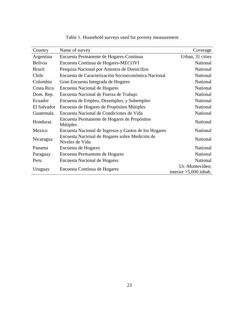
for all countries in LAC for which data are frequently collected during the 2003-14 period.14 Table
1 introduces all surveys (and their coverage) used in this paper.
12 See Castaneda et al. (2016), Bourguignon (2015), and Gasparini, Cicowiez, and Escudero (2013) for a more detailed
description of the SEDLAC project. 13 Since the main goal of the SEDLAC project is to enhance cross-country comparability, poverty measures in this
paper are not comparable to those published by NSOs in the region (Castaneda et al. 2016). 14 Guatemala and Nicaragua have fewer than four years of data and therefore they are excluded from the validation
(section 3) and sensitivity (section 4) analysis.
16
4.2 Empirical approach for testing and improving poverty nowcasting methods in LAC
We select a default value for all parameters used in the estimations. First, we assume a pass-
through 𝜃 = 1 for the NDG and QGC methods. Second, all past information is obtained from
periods -1 and -2 when nowcasting poverty in moment 0 –i.e., we compute 𝜖−1,−2 and Sq−1,−2
in
the PE and QGC methods respectively. Third, we set the number of quantiles q = 20 under the
QGC method.
In order to assess the validity of the three nowcasting techniques we compare the
nowcasted poverty rates in period 2005-14 with the actual poverty rates in all countries for which
poverty data are available more than three times in the period 2003-14. For instance, let’s assume
that we are interested in nowcasting poverty in 2005. Poverty nowcasted under the PE method is:
𝑃(𝑦2005)𝐸 = 𝑃(𝑦2004) ∗ (1 + 𝜖2004,2003 ∗ 𝑟𝑔2005,2004) (19)
Similarly, nowcasted incomes under the NDG method are:
�̃�𝑖𝑔2005 = 𝑦𝑖
2004 ∗ (1 + 𝑟𝑔2005,2004) (20)
Finally, incomes nowcasted under the QGC method are:
�̂�𝑖𝑞𝑔2005 =
𝑦𝑖𝑞2004
𝑌𝑞2004 ∗ (𝑆𝑞
2004,2003 ∗ 𝑟𝑔2005,2004 ∗ 𝑌2004 + 𝑌𝑞
2004) (21)
These results are compared with the actual poverty rate in 2005 in order to assess the
validity of the three methods. The same procedure is then repeated for all years in the 2006-14
period.15 Finally, we change the value of the default parameters –pass-through, periods used to
compute past information, and number of quantiles- in order to test the sensitivity of the estimates.
5 Validation of poverty nowcasting methods in LAC
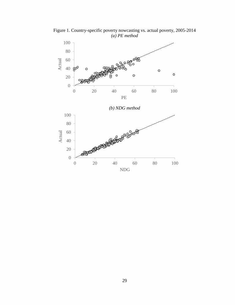
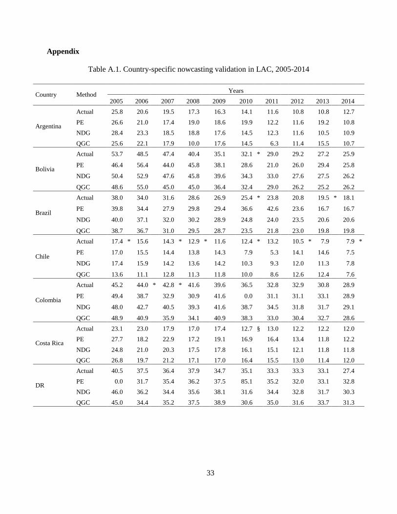
5.1 Country-specific validations
We start by comparing actual poverty estimates with the nowcasted poverty that is obtained from
applying all three methods described in previous sections. Figure 1 presents these comparisons for
all countries in LAC for which data are available between 2003 and 2014 on a regular basis (shown
in detail in appendix table A.1). In general, all methods perform reasonably well and all country-
specific poverty nowcasts are close to the actual poverty rates –i.e., all estimates are neighboring
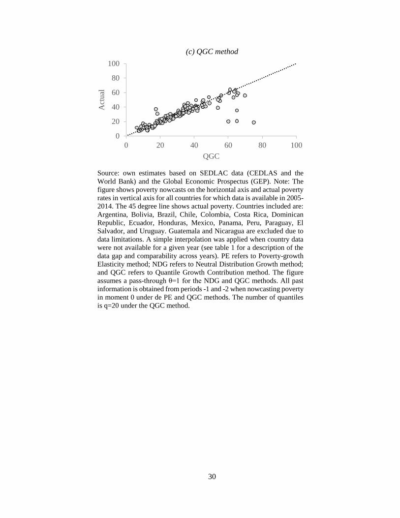
the 45 degree line. The NDG method performs better in most of the cases. We note that the QGC
15 We compare with an interpolated mid-point value whenever there is no actual poverty rate available.
17
and, in particular, the PE tend to be more dispersed around the 45 degree line and they have several
outliers in a number of cases.
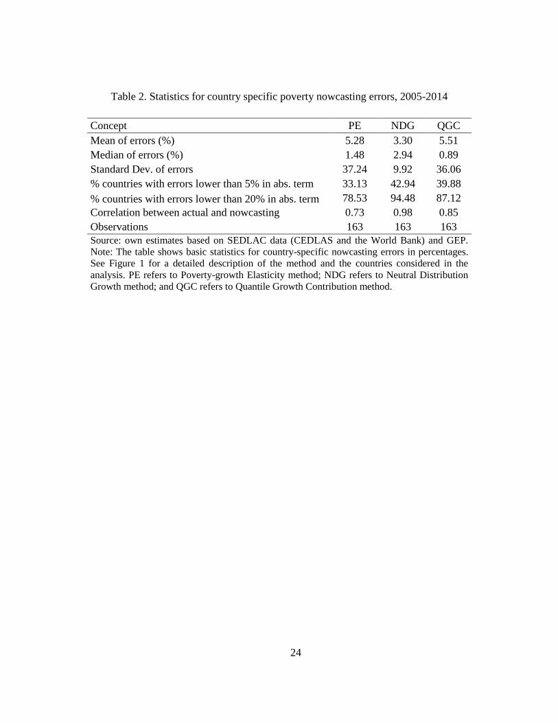
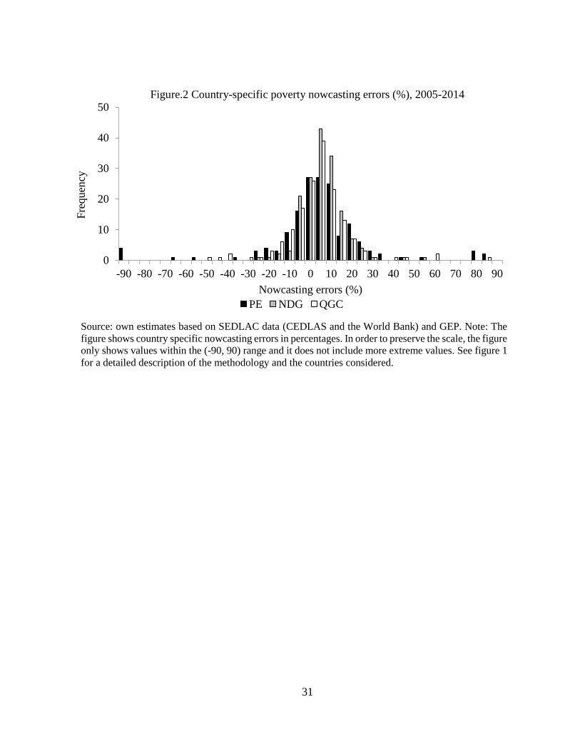
Table 2 and Figure 2 confirm these results. Table 2 shows a set of statistics of the
aggregated errors under the three methods, while Figure 2 presents the histogram of those errors.
Country-specific aggregate errors defined as the difference between poverty nowcasts and actual
poverty rates are quite small in general and the NDG tends to slightly outperform the other two
methods. On average, country-specific poverty nowcasts tend to be three percent higher than the
actual poverty rates under the NDG, while they tend to overstate actual poverty by about 5 percent
under the other two methods. As expected, the correlation between actual and nowcasted poverty
is higher under the NDG (0.98) than the QGC and PE methods (0.85 and 0.73, respectively).
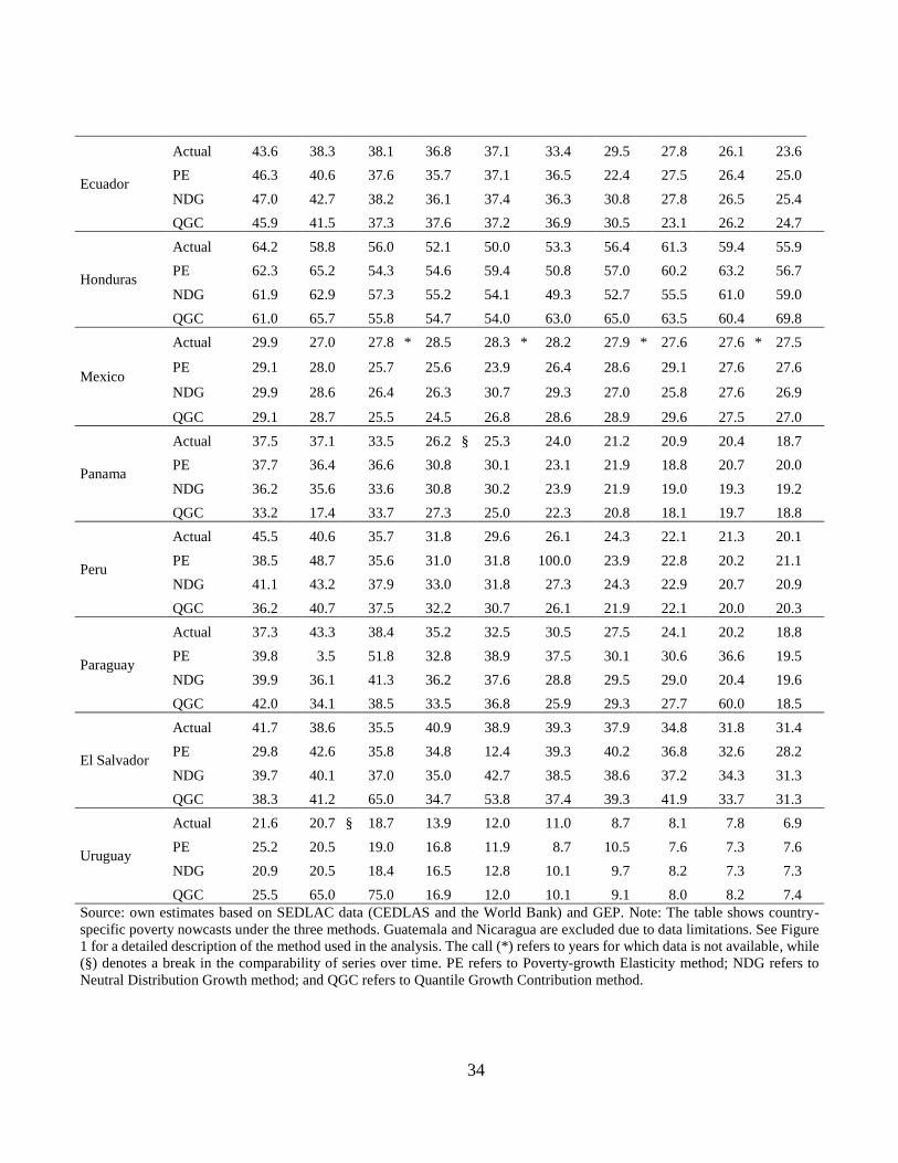
However, the QGC method outperforms the NDG once the outliers are taken into
consideration. The median of the nowcasting errors –a measure more robust to extreme values and
outliers- is about three times higher under the NDG when compared with the other two methods.
Therefore, good use of past information is key to produce nowcasts of good quality –i.e., to
minimize the IE- under the PE and QGC methods.16
Table 2 and Figure 2 also confirm a higher dispersion of poverty nowcasting errors under
the PE and QGC methods; the standard deviation of country level errors is about four times higher
than those of the NDG method. However, even when having large dispersion, errors under the
QGC tend to be more concentrated around zero than the PE. More than 87 percent of the cases
analyzed have nowcasting errors lower than 20 percent in absolute terms under the QGC and the
NDG methods, while less than 79 percent of the cases under the PE method.
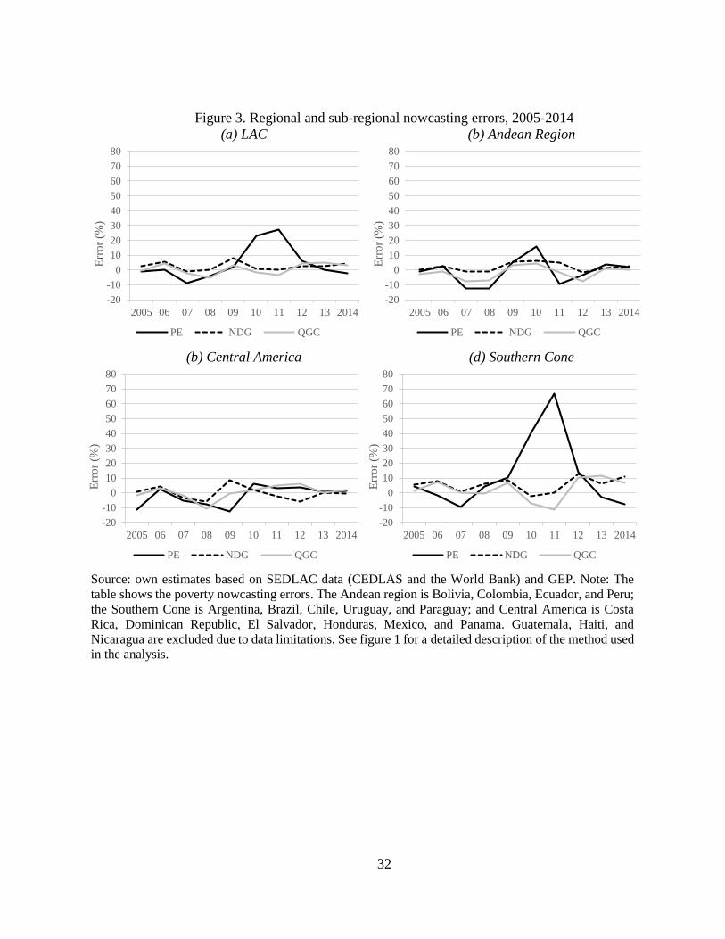
5.2 Regional and sub-regional level validations
At the regional and sub-regional levels, the performance of the methods differs from the country
level one. Table 3 shows actual and nowcasted regional and sub-regional poverty estimates under
the three methods for the period 2005-14, while Figure 3 shows the poverty nowcasting errors in
percentages. The three methods perform well in general terms. With the exception of Central
16 Since errors and outliers cannot be inferred in advance, outliers cannot be removed ex-ante. However, presenting
the median highlights the fact that NDG outperforms QGC in absence of the outliers produced by the latter method.
In addition, the table also shows that Elasticity is outperformed by the other two methods even after considering
outliers. Moreover, Table 2 helps understanding the risks associated with both QGC and PE methods in terms of the
outliers that may result from using past information.
18
America, correlation between nowcasting and actual poverty estimates are above 70 percent under
the three methods, and over 0.90 for the NDG and the QGC.
PE tends to be outpaced by the other two methods. Aggregate errors, defined as the
difference between poverty nowcasts and actual poverty rates, are quite small in general. In fact,
the QGC performs slightly better than the NDG method when computing regional poverty
nowcasts. For instance, the LAC average errors are about 1, 3, and 4 percent under the QGC, NDG,
and PE methods, respectively. Once again, the PE and the QGC are relatively more dispersed than
the GND.
Results under the QGC and NDG methods are encouraging both at the country and the
regional levels. Validations show a good performance of both methods. The next section presents
a series of sensitivity tests to changes in the default underlying parameters.
6 Stress and sensitivity analysis of poverty nowcasting methods in LAC
In this section we test the robustness of the findings to changes in the underlying parameters –i.e.,
past information, pass-through, and number of quantiles used when nowcasting regional and
country-level poverty rates. We perform all these test on the 15 countries for which data are
available on a regular basis and for LAC as a whole.
6.1 Sensitivity analysis of the Informational Error
The PE and QGC validation results use information on poverty elasticity and contribution to
growth from periods -2 and -1 when nowcasting poverty in moment 0. However, with few
exceptions, the 15 countries used in the analysis have micro data available on a yearly basis since
2003. This allows us to test whether the time span matters. For instance, we are interested in testing
whether results are improved when using poverty elasticity and quantile contribution to growth
between 2011-13 instead of 2012-13 when nowcasting poverty in 2014. The objective is to study
the sensitivity of the PE to changes in the length of the period used to estimate the poverty elasticity
and the quantile contribution to growth.
Table 4 shows 2014 poverty nowcasts for a range of periods for QGC and PE and keeping
everything else unchanged. The table shows that the methods perform similarly irrespective of the
length of periods used to estimate elasticity and growth contribution. However, there are a few
exceptions for both QGC and PE, which can lead to outliers like the ones observed in Figure 1.
For instance, QGC nowcasts increase significantly from 7.6 percent to 55 percent in Chile when
19
using the 2013-11 period instead of the 2013-12 one. Therefore, as mentioned in the previous
section, these exceptions reinforce the idea that past information is key to produce nowcasts of
good quality under the PE and QGC methods.
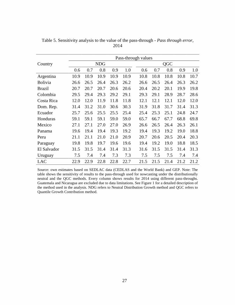
6.2 Sensitivity analysis of the Pass-through Error
All previous poverty nowcasts under the QGC and NDG were computed using a pass-through 𝜃 =
1. However, any value selected would be arbitrary since income growth from surveys tends to
differ from GDP per capita growth. Table 5 analyzes the sensitivity of 2014 nowcasts to the value
of the pass-through. The objective is to study the sensitivity of the PTE to changes in the pass-
through value keeping everything else unchanged. In general, the two methods perform similarly
irrespective of the value of the pass-through selected and results are robust to the underlying
assumption of the value of the pass-through.
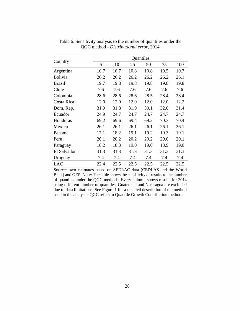
6.3 Sensitivity analysis of Distributional Error
Poverty nowcasts in section 4 were done using 20 quantiles under the QGC method. A relevant
question is whether the QGC performs well at nowcasting regional and sub-regional poverty
estimates when changing the number of quantiles. Table 6 shows 2014 poverty nowcasts using a
large set of quantiles from 5 to 100 and keeping everything else unchanged. The objective is to
study the sensitivity of the DE to changes in the number of quantiles. In general, the QGC method
performs similarly irrespective of the number of quantiles selected.
7 Conclusions
LAC has witnessed an impressive poverty reduction since 2003. Unfortunately, given that data are
usually available with more than one year lag in the region, we cannot say much yet about the
poverty impact of the lower economic growth that the region is currently experiencing. There are
several methods to forecast and nowcast poverty estimates, however little is known about their
level of accuracy and performance. To overcome this limitation, we use a comprehensive set of
about 180 harmonized micro household surveys available in 15 LAC countries from 2003 to 2014
to analyze the performance of three different forecasting methods: (i) the Poverty Elasticity (PE),
(ii) the Neutral Distribution Growth (NDG), and (iii) the Quantile Growth Contribution (QGC)
methods.
20
Results show that the three methods perform well at nowcasting large poverty reductions
as well as poverty stagnation in the region in the 2005-14 period. After comparing nowcasted with
actual poverty rates, in general we find the NDG and the QGC to be the best performers. However,
the PE and the QGC outperform the NDG once extreme values are taken into consideration,
meaning that good use of past information on poverty elasticities and quantile contributions to
growth is key for producing good quality poverty nowcasts under the PE and QGC methods. The
results are robust to a broad range of stress and sensitivity tests to changes in the underlying
parameters.
The use of validated methods for poverty nowcasting by researches and international
organizations is scarce, which is surprising in light of the massive acceptance that some of these
techniques have in closely related areas (for instance, for nowcasting GDP estimates). For this
reason, we stayed as close as possible to the standard nowcasting literature, relegating more
sophisticated approaches, such as the use of satellite data to produce real-time poverty information,
for further research. Our validation results provide support to the implementation of these methods
for poverty nowcasting, which is for guiding the regional debate on poverty measurement in LAC.
21
References
Alesina, Alberto, and Eliana La Ferrara. 1999. “Participation in Heterogeneous Communities.”
Working Paper 7155. National Bureau of Economic Research.
http://www.nber.org/papers/w7155.
Blix, M., Wadefjord, J., Wienecke, U., & Adahl, M. (2001). “How good is the forecasting
performance of major institutions?” sveriges riksbank economic review, 38-68.
Bourguignon, F. 2015. “Appraising income inequality databases in Latin America” The Journal
of Economic Inequality 13 (4): 557–578.
Carter, Michael R., Peter D. Little, Tewodaj Mogues, and Workneh Negatu. 2007. “Poverty
Traps and Natural Disasters in Ethiopia and Honduras.” World Development 35 (5): 835–
56. doi:10.1016/j.worlddev.2006.09.010.
Caruso, German; Castaneda Aguilar, Raul Andres; Lucchetti, Leonardo Ramiro. 2016. “Poverty
Nowcasting Methodologies” Working paper. Washington, D.C.: World Bank Group.
Castaneda Aguilar, Raul Andres; Gasparini, Leonardo Carlos; Garriga, Santiago; Lucchetti,
Leonardo Ramiro; Valderrama Gonzalez, Daniel. 2016. “Measuring poverty in Latin
America and the Caribbean: methodological considerations when estimating an empirical
regional poverty line.” Policy Research working paper; no. WPS 7621. Washington,
D.C.: World Bank Group.
Chandy, Laurence, Natasha Ledlie, and Veronika Penciakova. 2013. “The Final Countdown:
Prospects for Ending Extreme Poverty by 2030.” Global Views. Washington, D.C.: The
Brookings Institution.
Chen, Shaohua, and Martin Ravallion. 2001. “How Did the World’s Poorest Fare in the 1990s?”
The Review of Income and Wealth 47 (3): 283–300. doi:10.1111/1475-4991.00018.
Clemen, R. T. (1989). Combining forecasts: A review and annotated bibliography. International
journal of forecasting, 5(4), 559-583.
Chandy, Laurence, Natasha Ledlie, and Veronika Penciakova. 2013. “The Final Countdown:
Prospects for Ending Extreme Poverty by 2030.” Global Views. Washington, D.C.: The
Brookings Institution.
Cord, Louise, Oscar Barriga-Cabanillas, Leonardo Lucchetti, Carlos Rodríguez-Castelán, Liliana
D. Sousa, and Daniel Valderrama. 2017. “Inequality Stagnation in Latin America in the
Aftermath of the Global Financial Crisis.” Review of Development Economics 21 (1):
157–81. doi:10.1111/rode.12260.
Datt, Gaurav, and Martin Ravallion. 1992. “Growth and Redistribution Components of Changes
in Poverty Measures: A Decomposition with Applications to Brazil and India in the
1980s.” Journal of Development Economics 38 (2): 275–95. doi:10.1016/0304-
3878(92)90001-P.
Dollar, David, and Aart Kraay. 2002. “Growth Is Good for the Poor.” Journal of Economic
Growth 7 (3): 195–225. doi:10.1023/A:1020139631000.
Edward, Peter. 2006. “Examining Inequality: Who Really Benefits from Global Growth?” World
Development 34 (10): 1667–95. doi:10.1016/j.worlddev.2006.02.006.
Edward, Peter, and Andy Sumner. 2013. “The Future of Global Poverty in a Multi-Speed World:
New Estimates of Scale and Location, 2010-2030.” SSRN Scholarly Paper ID 2364153.
Rochester, NY: Social Science Research Network.
http://papers.ssrn.com/abstract=2364153.
22
Kakwani, Nanak. 1993. “Poverty and Economic Growth with Application to Côte D’ivoire.”
Review of Income and Wealth 39 (2): 121–39. doi:10.1111/j.1475-4991.1993.tb00443.x.
Karver, Jonathan, Charles Kenny, and Andy Sumner. 2012. “MDGS 2.0: What Goals, Targets,
and Timeframe?” IDS Working Papers 2012 (398): 1–57. doi:10.1111/j.2040-
0209.2012.00398.x.
Kraay, Aart. 2006. “When Is Growth pro-Poor? Evidence from a Panel of Countries.” Journal of
Development Economics 80 (1): 198–227. doi:10.1016/j.jdeveco.2005.02.004.
Ravallion, Martin. 2012. “Benchmarking Global Poverty Reduction.” SSRN Scholarly Paper ID
2150038. Rochester, NY: Social Science Research Network.
http://papers.ssrn.com/abstract=2150038.
———. 2013. “How Long Will It Take to Lift One Billion People Out of Poverty?” The World
Bank Research Observer 28 (2): 139–58. doi:10.1093/wbro/lkt003.
———. 2016. The Economics of Poverty: History, Measurement, and Policy. 1 edition. Oxford
University Press.
Ravallion, Martin, and Shaohua Chen. 1997. “What Can New Survey Data Tell Us about Recent
Changes in Distribution and Poverty?” The World Bank Economic Review 11 (2): 357–
82. doi:10.1093/wber/11.2.357.
The World Bank. 2000. “Global Economic Prospects and the Developing Countries.” Global
Economic Prospects. Washington, DC: World Bank.
http://econ.worldbank.org/WBSITE/EXTERNAL/EXTDEC/EXTDECPROSPECTS/0,,c
ontentMDK:23102090~pagePK:64165401~piPK:64165026~theSitePK:476883,00.html.
White, Howard, and Edward Anderson. 2001. “Growth versus Distribution: Does the Pattern of
Growth Matter?” Development Policy Review 19 (3): 267–89. doi:10.1111/1467-
7679.00134.
Yoshida, N., Hiroki Uematsu, and Carlos E. Sobrado. 2014. “Is Extreme Poverty Going to End?
An Analytical Framework to Evaluate Progress in Ending Extreme Poverty.” SSRN
Scholarly Paper ID 2375459. Rochester, NY: Social Science Research Network.
http://papers.ssrn.com/abstract=2375459.
23
Table 1. Household surveys used for poverty measurement
Country Name of survey Coverage
Argentina Encuesta Permanente de Hogares-Continua Urban, 31 cities
Bolivia Encuesta Continua de Hogares-MECOVI National
Brazil Pesquisa Nacional por Amostra de Domicilios National
Chile Encuesta de Caracterización Socioeconómica Nacional National
Colombia Gran Encuesta Integrada de Hogares National
Costa Rica Encuesta Nacional de Hogares National
Dom. Rep. Encuesta Nacional de Fuerza de Trabajo National
Ecuador Encuesta de Empleo, Desempleo, y Subempleo National
El Salvador Encuesta de Hogares de Propósitos Mútiples National
Guatemala Encuesta Nacional de Condiciones de Vida National
Honduras Encuesta Permanente de Hogares de Propósitos
Mútiples National
Mexico Encuesta Nacional de Ingresos y Gastos de los Hogares National
Nicaragua Encuesta Nacional de Hogares sobre Medición de
Niveles de Vida National
Panama Encuesta de Hogares National
Paraguay Encuesta Permanente de Hogares National
Peru Encuesta Nacional de Hogares National
Uruguay Encuesta Contínua de Hogares Ur.-Montevideo;
interior >5,000 inhab.
24
Table 2. Statistics for country specific poverty nowcasting errors, 2005-2014
Concept PE NDG QGC
Mean of errors (%) 5.28 3.30 5.51
Median of errors (%) 1.48 2.94 0.89
Standard Dev. of errors 37.24 9.92 36.06
% countries with errors lower than 5% in abs. term 33.13 42.94 39.88
% countries with errors lower than 20% in abs. term 78.53 94.48 87.12
Correlation between actual and nowcasting 0.73 0.98 0.85
Observations 163 163 163
Source: own estimates based on SEDLAC data (CEDLAS and the World Bank) and GEP.
Note: The table shows basic statistics for country-specific nowcasting errors in percentages.
See Figure 1 for a detailed description of the method and the countries considered in the
analysis. PE refers to Poverty-growth Elasticity method; NDG refers to Neutral Distribution
Growth method; and QGC refers to Quantile Growth Contribution method.
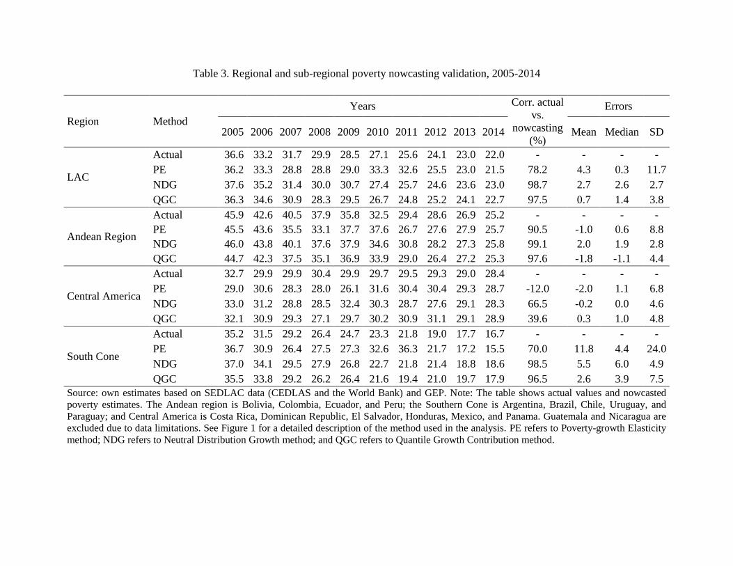
Table 3. Regional and sub-regional poverty nowcasting validation, 2005-2014
Region Method
Years Corr. actual
vs.
nowcasting
(%)
Errors
2005 2006 2007 2008 2009 2010 2011 2012 2013 2014 Mean Median SD
LAC
Actual 36.6 33.2 31.7 29.9 28.5 27.1 25.6 24.1 23.0 22.0 - - - -
PE 36.2 33.3 28.8 28.8 29.0 33.3 32.6 25.5 23.0 21.5 78.2 4.3 0.3 11.7
NDG 37.6 35.2 31.4 30.0 30.7 27.4 25.7 24.6 23.6 23.0 98.7 2.7 2.6 2.7
QGC 36.3 34.6 30.9 28.3 29.5 26.7 24.8 25.2 24.1 22.7 97.5 0.7 1.4 3.8
Andean Region
Actual 45.9 42.6 40.5 37.9 35.8 32.5 29.4 28.6 26.9 25.2 - - - -
PE 45.5 43.6 35.5 33.1 37.7 37.6 26.7 27.6 27.9 25.7 90.5 -1.0 0.6 8.8
NDG 46.0 43.8 40.1 37.6 37.9 34.6 30.8 28.2 27.3 25.8 99.1 2.0 1.9 2.8
QGC 44.7 42.3 37.5 35.1 36.9 33.9 29.0 26.4 27.2 25.3 97.6 -1.8 -1.1 4.4
Central America
Actual 32.7 29.9 29.9 30.4 29.9 29.7 29.5 29.3 29.0 28.4 - - - -
PE 29.0 30.6 28.3 28.0 26.1 31.6 30.4 30.4 29.3 28.7 -12.0 -2.0 1.1 6.8
NDG 33.0 31.2 28.8 28.5 32.4 30.3 28.7 27.6 29.1 28.3 66.5 -0.2 0.0 4.6
QGC 32.1 30.9 29.3 27.1 29.7 30.2 30.9 31.1 29.1 28.9 39.6 0.3 1.0 4.8
South Cone
Actual 35.2 31.5 29.2 26.4 24.7 23.3 21.8 19.0 17.7 16.7 - - - -
PE 36.7 30.9 26.4 27.5 27.3 32.6 36.3 21.7 17.2 15.5 70.0 11.8 4.4 24.0
NDG 37.0 34.1 29.5 27.9 26.8 22.7 21.8 21.4 18.8 18.6 98.5 5.5 6.0 4.9
QGC 35.5 33.8 29.2 26.2 26.4 21.6 19.4 21.0 19.7 17.9 96.5 2.6 3.9 7.5
Source: own estimates based on SEDLAC data (CEDLAS and the World Bank) and GEP. Note: The table shows actual values and nowcasted
poverty estimates. The Andean region is Bolivia, Colombia, Ecuador, and Peru; the Southern Cone is Argentina, Brazil, Chile, Uruguay, and
Paraguay; and Central America is Costa Rica, Dominican Republic, El Salvador, Honduras, Mexico, and Panama. Guatemala and Nicaragua are
excluded due to data limitations. See Figure 1 for a detailed description of the method used in the analysis. PE refers to Poverty-growth Elasticity
method; NDG refers to Neutral Distribution Growth method; and QGC refers to Quantile Growth Contribution method.
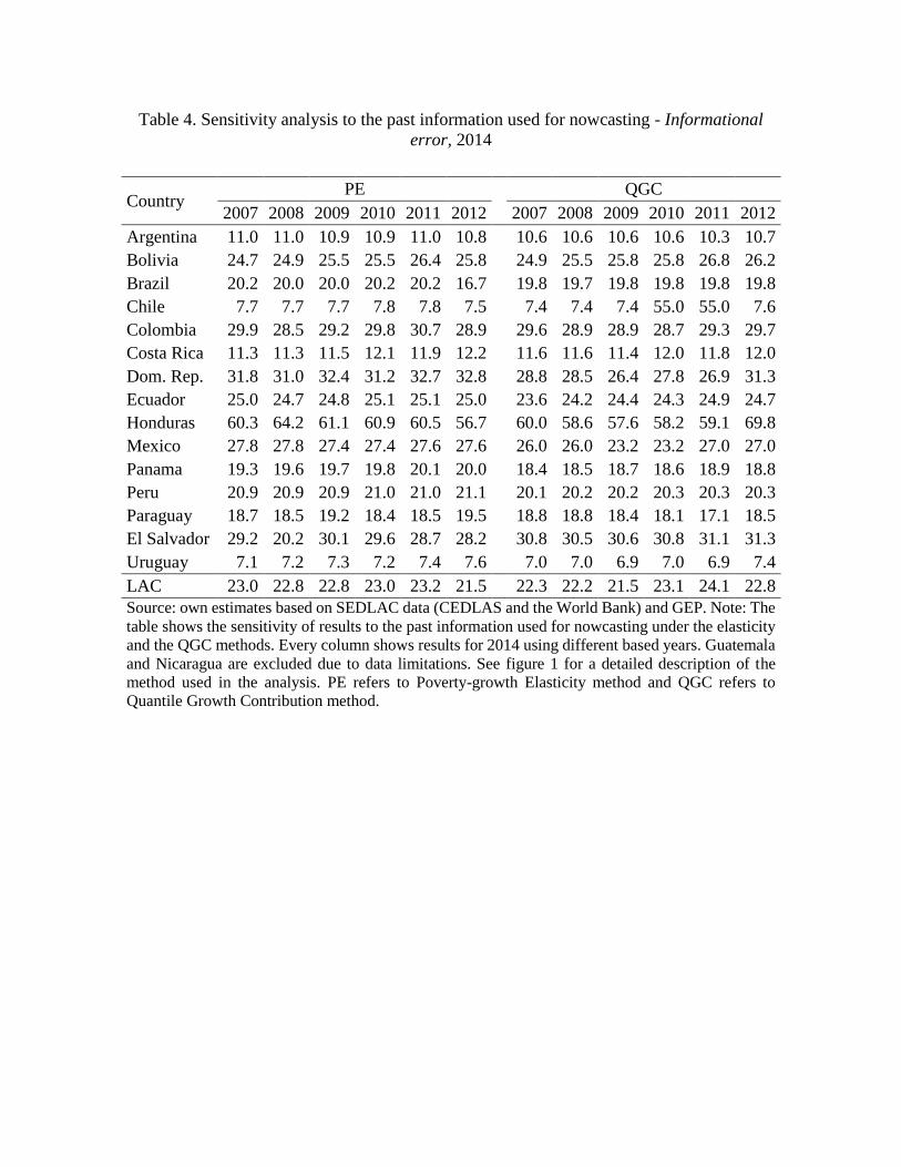
Table 4. Sensitivity analysis to the past information used for nowcasting - Informational
error, 2014
Country PE QGC
2007 2008 2009 2010 2011 2012 2007 2008 2009 2010 2011 2012
Argentina 11.0 11.0 10.9 10.9 11.0 10.8 10.6 10.6 10.6 10.6 10.3 10.7
Bolivia 24.7 24.9 25.5 25.5 26.4 25.8 24.9 25.5 25.8 25.8 26.8 26.2
Brazil 20.2 20.0 20.0 20.2 20.2 16.7 19.8 19.7 19.8 19.8 19.8 19.8
Chile 7.7 7.7 7.7 7.8 7.8 7.5 7.4 7.4 7.4 55.0 55.0 7.6
Colombia 29.9 28.5 29.2 29.8 30.7 28.9 29.6 28.9 28.9 28.7 29.3 29.7
Costa Rica 11.3 11.3 11.5 12.1 11.9 12.2 11.6 11.6 11.4 12.0 11.8 12.0
Dom. Rep. 31.8 31.0 32.4 31.2 32.7 32.8 28.8 28.5 26.4 27.8 26.9 31.3
Ecuador 25.0 24.7 24.8 25.1 25.1 25.0 23.6 24.2 24.4 24.3 24.9 24.7
Honduras 60.3 64.2 61.1 60.9 60.5 56.7 60.0 58.6 57.6 58.2 59.1 69.8
Mexico 27.8 27.8 27.4 27.4 27.6 27.6 26.0 26.0 23.2 23.2 27.0 27.0
Panama 19.3 19.6 19.7 19.8 20.1 20.0 18.4 18.5 18.7 18.6 18.9 18.8
Peru 20.9 20.9 20.9 21.0 21.0 21.1 20.1 20.2 20.2 20.3 20.3 20.3
Paraguay 18.7 18.5 19.2 18.4 18.5 19.5 18.8 18.8 18.4 18.1 17.1 18.5
El Salvador 29.2 20.2 30.1 29.6 28.7 28.2 30.8 30.5 30.6 30.8 31.1 31.3
Uruguay 7.1 7.2 7.3 7.2 7.4 7.6 7.0 7.0 6.9 7.0 6.9 7.4
LAC 23.0 22.8 22.8 23.0 23.2 21.5 22.3 22.2 21.5 23.1 24.1 22.8
Source: own estimates based on SEDLAC data (CEDLAS and the World Bank) and GEP. Note: The
table shows the sensitivity of results to the past information used for nowcasting under the elasticity
and the QGC methods. Every column shows results for 2014 using different based years. Guatemala
and Nicaragua are excluded due to data limitations. See figure 1 for a detailed description of the
method used in the analysis. PE refers to Poverty-growth Elasticity method and QGC refers to
Quantile Growth Contribution method.
27
Table 5. Sensitivity analysis to the value of the pass-through - Pass through error,
2014
Country
Pass-through values
NDG QGC
0.6 0.7 0.8 0.9 1.0 0.6 0.7 0.8 0.9 1.0
Argentina 10.9 10.9 10.9 10.9 10.9 10.8 10.8 10.8 10.8 10.7
Bolivia 26.6 26.5 26.4 26.3 26.2 26.6 26.5 26.4 26.3 26.2
Brazil 20.7 20.7 20.7 20.6 20.6 20.4 20.2 20.1 19.9 19.8
Colombia 29.5 29.4 29.3 29.2 29.1 29.3 29.1 28.9 28.7 28.6
Costa Rica 12.0 12.0 11.9 11.8 11.8 12.1 12.1 12.1 12.0 12.0
Dom. Rep. 31.4 31.2 31.0 30.6 30.3 31.9 31.8 31.7 31.4 31.3
Ecuador 25.7 25.6 25.5 25.5 25.4 25.4 25.3 25.1 24.8 24.7
Honduras 59.1 59.1 59.1 59.0 59.0 65.7 66.7 67.7 68.8 69.8
Mexico 27.1 27.1 27.0 27.0 26.9 26.6 26.5 26.4 26.3 26.1
Panama 19.6 19.4 19.4 19.3 19.2 19.4 19.3 19.2 19.0 18.8
Peru 21.1 21.1 21.0 21.0 20.9 20.7 20.6 20.5 20.4 20.3
Paraguay 19.8 19.8 19.7 19.6 19.6 19.4 19.2 19.0 18.8 18.5
El Salvador 31.5 31.5 31.4 31.4 31.3 31.6 31.5 31.5 31.4 31.3
Uruguay 7.5 7.4 7.4 7.3 7.3 7.5 7.5 7.5 7.4 7.4
LAC 22.9 22.9 22.8 22.8 22.7 21.5 21.5 21.4 21.2 21.2
Source: own estimates based on SEDLAC data (CEDLAS and the World Bank) and GEP. Note: The
table shows the sensitivity of results to the pass-through used for nowcasting under the distributionally
neutral and the QGC methods. Every column shows results for 2014 using different pass-throughs.
Guatemala and Nicaragua are excluded due to data limitations. See Figure 1 for a detailed description of
the method used in the analysis. NDG refers to Neutral Distribution Growth method and QGC refers to
Quantile Growth Contribution method.
28
Table 6. Sensitivity analysis to the number of quantiles under the
QGC method - Distributional error, 2014
Country Quantiles
5 10 25 50 75 100
Argentina 10.7 10.7 10.8 10.8 10.5 10.7
Bolivia 26.2 26.2 26.2 26.2 26.2 26.1
Brazil 19.7 19.8 19.8 19.8 19.8 19.8
Chile 7.6 7.6 7.6 7.6 7.6 7.6
Colombia 28.6 28.6 28.6 28.5 28.4 28.4
Costa Rica 12.0 12.0 12.0 12.0 12.0 12.2
Dom. Rep. 31.9 31.8 31.9 30.1 32.0 31.4
Ecuador 24.9 24.7 24.7 24.7 24.7 24.7
Honduras 69.2 69.6 69.4 69.2 70.3 70.4
Mexico 26.1 26.1 26.1 26.1 26.1 26.1
Panama 17.1 18.2 19.1 19.2 19.3 19.1
Peru 20.1 20.2 20.2 20.2 20.0 20.1
Paraguay 18.2 18.3 19.0 19.0 18.9 19.0
El Salvador 31.3 31.3 31.3 31.3 31.3 31.3
Uruguay 7.4 7.4 7.4 7.4 7.4 7.4
LAC 22.4 22.5 22.5 22.5 22.5 22.5
Source: own estimates based on SEDLAC data (CEDLAS and the World
Bank) and GEP. Note: The table shows the sensitivity of results to the number
of quantiles under the QGC methods. Every column shows results for 2014
using different number of quantiles. Guatemala and Nicaragua are excluded
due to data limitations. See Figure 1 for a detailed description of the method
used in the analysis. QGC refers to Quantile Growth Contribution method.
29
Figure 1. Country-specific poverty nowcasting vs. actual poverty, 2005-2014
(a) PE method
(b) NDG method
0
20
40
60
80
100
0 20 40 60 80 100
Act
ual
PE
0
20
40
60
80
100
0 20 40 60 80 100
Act
ual
NDG
30
(c) QGC method
Source: own estimates based on SEDLAC data (CEDLAS and the
World Bank) and the Global Economic Prospectus (GEP). Note: The
figure shows poverty nowcasts on the horizontal axis and actual poverty
rates in vertical axis for all countries for which data is available in 2005-
2014. The 45 degree line shows actual poverty. Countries included are:
Argentina, Bolivia, Brazil, Chile, Colombia, Costa Rica, Dominican
Republic, Ecuador, Honduras, Mexico, Panama, Peru, Paraguay, El
Salvador, and Uruguay. Guatemala and Nicaragua are excluded due to
data limitations. A simple interpolation was applied when country data
were not available for a given year (see table 1 for a description of the
data gap and comparability across years). PE refers to Poverty-growth
Elasticity method; NDG refers to Neutral Distribution Growth method;
and QGC refers to Quantile Growth Contribution method. The figure
assumes a pass-through θ=1 for the NDG and QGC methods. All past
information is obtained from periods -1 and -2 when nowcasting poverty
in moment 0 under de PE and QGC methods. The number of quantiles
is q=20 under the QGC method.
0
20
40
60
80
100
0 20 40 60 80 100
Act
ual
QGC
31
Figure.2 Country-specific poverty nowcasting errors (%), 2005-2014
Source: own estimates based on SEDLAC data (CEDLAS and the World Bank) and GEP. Note: The
figure shows country specific nowcasting errors in percentages. In order to preserve the scale, the figure
only shows values within the (-90, 90) range and it does not include more extreme values. See figure 1
for a detailed description of the methodology and the countries considered.
-90 -80 -70 -60 -50 -40 -30 -20 -10 0 10 20 30 40 50 60 70 80 90
0
10
20
30
40
50
Nowcasting errors (%)
Fre
quen
cy
PE NDG QGC
32
Figure 3. Regional and sub-regional nowcasting errors, 2005-2014
(a) LAC (b) Andean Region
(b) Central America (d) Southern Cone
Source: own estimates based on SEDLAC data (CEDLAS and the World Bank) and GEP. Note: The
table shows the poverty nowcasting errors. The Andean region is Bolivia, Colombia, Ecuador, and Peru;
the Southern Cone is Argentina, Brazil, Chile, Uruguay, and Paraguay; and Central America is Costa
Rica, Dominican Republic, El Salvador, Honduras, Mexico, and Panama. Guatemala, Haiti, and
Nicaragua are excluded due to data limitations. See figure 1 for a detailed description of the method used
in the analysis.
-20
-10
0
10
20
30
40
50
60
70
80
2005 06 07 08 09 10 11 12 13 2014
Err
or
(%)
PE NDG QGC
-20
-10
0
10
20
30
40
50
60
70
80
2005 06 07 08 09 10 11 12 13 2014
Err
or
(%)
PE NDG QGC
-20
-10
0
10
20
30
40
50
60
70
80
2005 06 07 08 09 10 11 12 13 2014
Err
or
(%)
PE NDG QGC
-20
-10
0
10
20
30
40
50
60
70
80
2005 06 07 08 09 10 11 12 13 2014
Err
or
(%)
PE NDG QGC
33
Appendix
Table A.1. Country-specific nowcasting validation in LAC, 2005-2014
Country Method Years
2005 2006 2007 2008 2009 2010 2011 2012 2013 2014
Argentina
Actual 25.8 20.6 19.5 17.3 16.3 14.1 11.6 10.8 10.8 12.7
PE 26.6 21.0 17.4 19.0 18.6 19.9 12.2 11.6 19.2 10.8
NDG 28.4 23.3 18.5 18.8 17.6 14.5 12.3 11.6 10.5 10.9
QGC 25.6 22.1 17.9 10.0 17.6 14.5 6.3 11.4 15.5 10.7
Bolivia
Actual 53.7 48.5 47.4 40.4 35.1 32.1 * 29.0 29.2 27.2 25.9
PE 46.4 56.4 44.0 45.8 38.1 28.6 21.0 26.0 29.4 25.8
NDG 50.4 52.9 47.6 45.8 39.6 34.3 33.0 27.6 27.5 26.2
QGC 48.6 55.0 45.0 45.0 36.4 32.4 29.0 26.2 25.2 26.2
Brazil
Actual 38.0 34.0 31.6 28.6 26.9 25.4 * 23.8 20.8 19.5 * 18.1
PE 39.8 34.4 27.9 29.8 29.4 36.6 42.6 23.6 16.7 16.7
NDG 40.0 37.1 32.0 30.2 28.9 24.8 24.0 23.5 20.6 20.6
QGC 38.7 36.7 31.0 29.5 28.7 23.5 21.8 23.0 19.8 19.8
Chile
Actual 17.4 * 15.6 14.3 * 12.9 * 11.6 12.4 * 13.2 10.5 * 7.9 7.9 *
PE 17.0 15.5 14.4 13.8 14.3 7.9 5.3 14.1 14.6 7.5
NDG 17.4 15.9 14.2 13.6 14.2 10.3 9.3 12.0 11.3 7.8
QGC 13.6 11.1 12.8 11.3 11.8 10.0 8.6 12.6 12.4 7.6
Colombia
Actual 45.2 44.0 * 42.8 * 41.6 39.6 36.5 32.8 32.9 30.8 28.9
PE 49.4 38.7 32.9 30.9 41.6 0.0 31.1 31.1 33.1 28.9
NDG 48.0 42.7 40.5 39.3 41.6 38.7 34.5 31.8 31.7 29.1
QGC 48.9 40.9 35.9 34.1 40.9 38.3 33.0 30.4 32.7 28.6
Costa Rica
Actual 23.1 23.0 17.9 17.0 17.4 12.7 § 13.0 12.2 12.2 12.0
PE 27.7 18.2 22.9 17.2 19.1 16.9 16.4 13.4 11.8 12.2
NDG 24.8 21.0 20.3 17.5 17.8 16.1 15.1 12.1 11.8 11.8
QGC 26.8 19.7 21.2 17.1 17.0 16.4 15.5 13.0 11.4 12.0
DR
Actual 40.5 37.5 36.4 37.9 34.7 35.1 33.3 33.3 33.1 27.4
PE 0.0 31.7 35.4 36.2 37.5 85.1 35.2 32.0 33.1 32.8
NDG 46.0 36.2 34.4 35.6 38.1 31.6 34.4 32.8 31.7 30.3
QGC 45.0 34.4 35.2 37.5 38.9 30.6 35.0 31.6 33.7 31.3
34
Ecuador
Actual 43.6 38.3 38.1 36.8 37.1 33.4 29.5 27.8 26.1 23.6
PE 46.3 40.6 37.6 35.7 37.1 36.5 22.4 27.5 26.4 25.0
NDG 47.0 42.7 38.2 36.1 37.4 36.3 30.8 27.8 26.5 25.4
QGC 45.9 41.5 37.3 37.6 37.2 36.9 30.5 23.1 26.2 24.7
Honduras
Actual 64.2 58.8 56.0 52.1 50.0 53.3 56.4 61.3 59.4 55.9
PE 62.3 65.2 54.3 54.6 59.4 50.8 57.0 60.2 63.2 56.7
NDG 61.9 62.9 57.3 55.2 54.1 49.3 52.7 55.5 61.0 59.0
QGC 61.0 65.7 55.8 54.7 54.0 63.0 65.0 63.5 60.4 69.8
Mexico
Actual 29.9 27.0 27.8 * 28.5 28.3 * 28.2 27.9 * 27.6 27.6 * 27.5
PE 29.1 28.0 25.7 25.6 23.9 26.4 28.6 29.1 27.6 27.6
NDG 29.9 28.6 26.4 26.3 30.7 29.3 27.0 25.8 27.6 26.9
QGC 29.1 28.7 25.5 24.5 26.8 28.6 28.9 29.6 27.5 27.0
Panama
Actual 37.5 37.1 33.5 26.2 § 25.3 24.0 21.2 20.9 20.4 18.7
PE 37.7 36.4 36.6 30.8 30.1 23.1 21.9 18.8 20.7 20.0
NDG 36.2 35.6 33.6 30.8 30.2 23.9 21.9 19.0 19.3 19.2
QGC 33.2 17.4 33.7 27.3 25.0 22.3 20.8 18.1 19.7 18.8
Peru
Actual 45.5 40.6 35.7 31.8 29.6 26.1 24.3 22.1 21.3 20.1
PE 38.5 48.7 35.6 31.0 31.8 100.0 23.9 22.8 20.2 21.1
NDG 41.1 43.2 37.9 33.0 31.8 27.3 24.3 22.9 20.7 20.9
QGC 36.2 40.7 37.5 32.2 30.7 26.1 21.9 22.1 20.0 20.3
Paraguay
Actual 37.3 43.3 38.4 35.2 32.5 30.5 27.5 24.1 20.2 18.8
PE 39.8 3.5 51.8 32.8 38.9 37.5 30.1 30.6 36.6 19.5
NDG 39.9 36.1 41.3 36.2 37.6 28.8 29.5 29.0 20.4 19.6
QGC 42.0 34.1 38.5 33.5 36.8 25.9 29.3 27.7 60.0 18.5
El Salvador
Actual 41.7 38.6 35.5 40.9 38.9 39.3 37.9 34.8 31.8 31.4
PE 29.8 42.6 35.8 34.8 12.4 39.3 40.2 36.8 32.6 28.2
NDG 39.7 40.1 37.0 35.0 42.7 38.5 38.6 37.2 34.3 31.3
QGC 38.3 41.2 65.0 34.7 53.8 37.4 39.3 41.9 33.7 31.3
Uruguay
Actual 21.6 20.7 § 18.7 13.9 12.0 11.0 8.7 8.1 7.8 6.9
PE 25.2 20.5 19.0 16.8 11.9 8.7 10.5 7.6 7.3 7.6
NDG 20.9 20.5 18.4 16.5 12.8 10.1 9.7 8.2 7.3 7.3
QGC 25.5 65.0 75.0 16.9 12.0 10.1 9.1 8.0 8.2 7.4
Source: own estimates based on SEDLAC data (CEDLAS and the World Bank) and GEP. Note: The table shows country-
specific poverty nowcasts under the three methods. Guatemala and Nicaragua are excluded due to data limitations. See Figure
1 for a detailed description of the method used in the analysis. The call (*) refers to years for which data is not available, while
(§) denotes a break in the comparability of series over time. PE refers to Poverty-growth Elasticity method; NDG refers to
Neutral Distribution Growth method; and QGC refers to Quantile Growth Contribution method.