Embed Size (px)
Citation preview

Business Statistics 41000:
Multiple Linear Regression
Drew D. Creal
University of Chicago, Booth School of Business
March 14 and 15, 2014
1

Class information
I Drew D. Creal
I Email: [email protected]
I Office: 404 Harper Center
I Office hours: email me for an appointment
I Office phone: 773.834.5249
http://faculty.chicagobooth.edu/drew.creal/teaching/index.html
2

Course schedule
I Week # 1: Plotting and summarizing univariate data
I Week # 2: Plotting and summarizing bivariate data
I Week # 3: Probability 1
I Week # 4: Probability 2
I Week # 5: Probability 3
I Week # 6: In-class exam and Probability 4
I Week # 7: Statistical inference 1
I Week # 8: Statistical inference 2
I Week # 9: Simple linear regression
I Week # 10: Multiple linear regression
3

Outline of today’s topics
I. The multiple linear regression model
II. Estimates and plug-in prediction
III. Confidence intervals and hypothesis tests
IV. Fitted values, residuals, R-squared
V. The overall F -test
VI. Using categorical variables as regressors
4

The Multiple Linear Regression Model
5

Multiple Linear Regression
The plug-in predictive interval for the price of a house given itssize is quite large.
Is this “bad”?
Not necessarily. You can’t accurately predict the price of ahouse just based on its size. The width of our predictiveinterval reflects this.
How can we predict the price of a house more accurately?
If we know more about a house, we should have a better ideaof its price!
6

Multiple Linear Regression
Here are the first 10 rows of our housing data (MidCity.xls).
Home Nbhd Offers SqFt Brick Bedrooms Bathrooms Price
1 2 2 1790 No 2 2 114300
2 2 3 2030 No 4 2 114200
3 2 1 1740 No 3 2 114800
4 2 3 1980 No 3 2 94700
5 2 3 2130 No 3 3 119800
6 1 2 1780 No 3 2 114600
7 3 3 1830 Yes 3 3 151600
8 3 2 2160 No 4 2 150700
9 2 3 2110 No 4 2 119200
10 2 3 1730 No 3 3 104000
Our data has more variables than just size and price.
For example, we also know the number of bedrooms andbathrooms each house has.
How do we incorporate this information?
7
Multiple Linear Regression
Home Nbhd Offers SqFt Brick Bedrooms Bathrooms Price
1 2 2 1790 No 2 2 114300
2 2 3 2030 No 4 2 114200
3 2 1 1740 No 3 2 114800
4 2 3 1980 No 3 2 94700
5 2 3 2130 No 3 3 119800
6 1 2 1780 No 3 2 114600
7 3 3 1830 Yes 3 3 151600
8 3 2 2160 No 4 2 150700
9 2 3 2110 No 4 2 119200
10 2 3 1730 No 3 3 104000
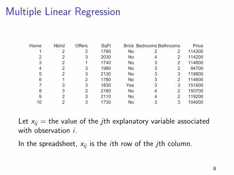
Let xij = the value of the jth explanatory variable associatedwith observation i .
In the spreadsheet, xij is the ith row of the jth column.
8

Multiple Linear Regression
The multiple linear regression model is
Yi = α + β1xi1 + β2xi2 + . . . + βkxik + εi .
εi ∼ N(0, σ2) i.i.d.
εi is independent of x1, x2, . . . , xk .
I Y is a linear combination of the k different x variables + “error”.
I The error works exactly the same way as in simple linear regression.We assume the ε are independent of all the x ’s.
9

Multiple Linear Regression: Remarks
Yi = α + β1xi1 + β2xi2 + . . . + βkxik + εi εi ∼ N(0, σ2)
I xij is the value of the j-th explanatory variable (orregressor) associated with observation i . There are kregressors.
I With k variables, we can no longer interpret a regressionas a line.
I α is still the intercept, our “guess” for Y when all the x ’s= 0.
I There are now k slope coefficients βj , one for each x .
10

Multiple Linear Regression: Remarks
Yi = α + β1xi1 + β2xi2 + . . . + βkxik + εi εi ∼ N(0, σ2)
How do we interpret the coefficients βj for j = 1, . . . , k?
IMPORTANT: The interpretation of the coefficients βjchanges.
Each coefficient βj now describes the change in Y when xiincreases by one unit, holding all of the other x’s fixed.
You can think of this as “controlling” for all of the other x ’s.
11
Multiple Linear Regression: Remarks
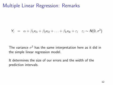
Yi = α + β1xi1 + β2xi2 + . . . + βkxik + εi εi ∼ N(0, σ2)
The variance σ2 has the same interpretation here as it did inthe simple linear regression model.
It determines the size of our errors and the width of theprediction intervals.
12

Regression as a model of
P(Y = y |X1 = x1, . . . ,Xk = xk)
13

Regression as a model of the cond. distribution
We should also think about the model as a model for theconditional distribution of Y given our x variables.
Y |X1 = x1, . . . ,Xk = xk ∼ N(µy |x , σ2)
The conditional distribution of Y given all of the x ’s is anormal distribution.
What are the conditional mean and variance?
I E[Y |X1 = x1, . . . ,Xk = xk ]
I V[Y |X1 = x1, . . . ,Xk = xk ]
14

Conditional mean
The multiple linear regression model
Yi = α + β1xi1 + β2xi2 + . . . + βkxik + εi εi ∼ N(0, σ2)
states that the conditional mean depends on the X ’s througha linear combination.
Using our formulas for linear combinations, we find that
E[Y |X1 = x1, . . . ,Xk = xk ] = α + β1x1 + β2x2 + . . . + βkxk
(Note: This only requires that E[εi ] = 0.)
15
Conditional mean
Our multiple linear regression model
Yi = α + β1xi1 + β2xi2 + . . . + βkxik + εi εi ∼ N(0, σ2)
states that the conditional variance is not a function of theX ’s.
Using our formulas for linear combinations, we find that
V[Y |X1 = x1, . . . ,Xk = xk ] = σ2
(Note: This only requires that V[εi |X ] = σ2.)
16
Prediction
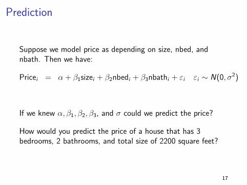
Suppose we model price as depending on size, nbed, andnbath. Then we have:
Pricei = α + β1sizei + β2nbedi + β3nbathi + εi εi ∼ N(0, σ2)
If we knew α, β1, β2, β3, and σ could we predict the price?
How would you predict the price of a house that has 3bedrooms, 2 bathrooms, and total size of 2200 square feet?
17

Prediction
How would you predict the price of a house that has 3bedrooms, 2 bathrooms, and total size of 2200 square feet?
Our prediction for the price of the house is
α + β1 ∗ 2200 + β2 ∗ 3 + β3 ∗ 2
Since ε is normal, a 95% prediction interval for the price is
(α+ β12200 + β23 + β32− 2σ, α + β12200 + β23 + β32 + 2σ)
18

Estimating α, βj , and σ
19

Multiple Linear Regression
Of course, we do not know α, β1, β2, β3 and σ. Instead, wehave to estimate them from observed data.
Pricei = α + β1sizei + β2nbedi + β3nbathi + εi εi ∼ N(0, σ2)
Given data, we can estimate the unknown “true” valuesα, β1, β2, β3, and σ.
I α is our estimate of α.
I β1, β2, and β3 are our estimates of β1, β2, and β3.
I se is our estimate of σ.
20

Estimators
For simple linear regression, we wrote down formulas for α andβ.
We could do that for multiple regression, too, but the formulasget more complex.
Typically, we express these formulas using matrix algebra.
We won’t go into the details. However, the estimates α and βjfor j = 1, . . . , k are still determined by the sample means,sample variances, and sample covariances.
21

Estimates
Here is the output of a multiple regression from Excel.
α = −5.64, β1 = 35.64, β2 = 10.45, β3 = 13.55 andse = 20.36.
22

Formula for the standard deviation
Our estimate of σ is just the sample standard deviation of theresiduals ei .
se =
√∑ni=1 e2
in−k−1
I Remember for simple regression, k = 1. This is really thesame formula. We divide by n − k − 1 for the samereason.
I se just asks, “on average, how far are our observed valuesyi away from our fitted values?”
23

Interpreting the estimates
For the housing data, our estimated fitted regression is
Pricei = −5.64 + 35.64sizei + 10.46nbedi + 13.55nbathi
So, for example, β2 = 10.46. How do we interpret this?
With size and nbath held fixed, how does adding onebedroom affect the value of the house?
Answer: adding a bedroom increases the price by $10,460.
24

Interpreting the estimates
Pricei = −5.64 + 35.64sizei + 10.46nbedi + 13.55nbathi
Another example, β1 = 35.64. How do we interpret this?
With nbed and nbath held fixed, how does adding 1000square feet affect the value of the house?
Answer: For a house that has the same nbed and nbath,adding 1000 square feet increases the price of the house by$35,640.
25

Using the estimates to predict
Suppose a house has size = 2.2, 3 bedrooms and 2 bathrooms.
What is your (estimated) prediction for its price?
−5.64 + 35.64 ∗ 2.2 + 10.46 ∗ 3 + 13.55 ∗ 2 = 131.248
Our prediction is $ 131,248.
26

Using the estimates to predict
Suppose a house has size = 2.2, 3 bedrooms and 2 bathrooms.
Can you provide a prediction interval for the price?
Given that se = 20.36, a 95% prediction interval for the price is
131.248± 2se = (90.53, 171.97)
This is our multiple regression “plug-in” predictive interval.We just plug in our estimates α, β1, β2, β3, and se in place ofthe unknown “true” parameters α, β1, β2, β3, and σ.
27

Estimates
Note # 1: Adding covariates can change our estimates.
When we regressed price on size the coefficient was about 70.
Now the coefficient for size is about 36.
Without nbath and nbed in the regression, an increase in sizecan by associated with an increase in nbath and nbed “in thebackground.”
If all I know is that one house is a lot bigger than another Imight expect the bigger house to have more beds and baths!
With nbath and nbed held fixed, the effect of size is smaller.
28

Estimates
Example: Suppose I build a 1000 square foot addition to myhouse. This addition includes two bedrooms and onebathroom.
How does this affect the value of my house?
35.64 ∗ 1 + 10.46 ∗ 2 + 13.55 ∗ 1 = 70.11
The value of the house goes up by $70,110. This is almostexactly the relationship we estimated before!
But now we can say, if the 1000 square foot addition is only abasement (rather than a new bed/bathroom) the increase invalue is much smaller. The new model is much more realistic.
29
Estimates
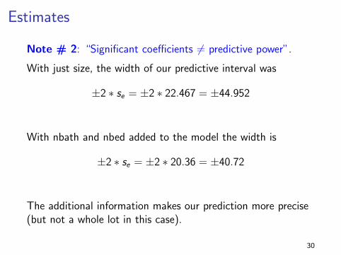
Note # 2: “Significant coefficients 6= predictive power”.
With just size, the width of our predictive interval was
±2 ∗ se = ±2 ∗ 22.467 = ±44.952
With nbath and nbed added to the model the width is
±2 ∗ se = ±2 ∗ 20.36 = ±40.72
The additional information makes our prediction more precise(but not a whole lot in this case).
30

Confidence Intervals and Hypothesis Tests
31

Standard Errors and Confidence Intervals
Remember, our estimate βj is not likely to be equal to the“true” unknown value βj .
This is due to sampling error.
Remember that we could observe a different sample of houses,which would cause us to get different estimates βj .
We measure our uncertainty about βj using the standard errorsβj , which is the standard deviation of the sampling
distribution of βj .
32

The Sampling Distribution of an Estimator
The sampling distribution of an estimator is aprobability distribution that describes allthe possible values we might see if we could“repeat” our sample over and over again; i.e., if wecould see other potential samples from thepopulation we are studying.
33

Sampling Distributions for α and βj
Due to the CLT, the sampling distributions for the estimatorsare normal distributions.
However, you will often see confidence intervals for α and βconstructed using the Student’s t distribution instead of thestandard normal.
The reasoning behind this is because we “standardize” eachestimator, when we form our test statistic (see Lecture #8).
Again, we are “standardizing” the estimators α and βj tocompute the test statistic. This means we are dividing themby the standard errors sα and sβj , which need to be estimatedfrom the data.
34

Confidence Intervals
The 95% confidence interval for α is
α± tval ∗ sα
where tval = TINV(0.05, n − k − 1) (NOTE: in Excel)
The 95% confidence interval for βj is
βj ± tval ∗ sβj
where tval = TINV(0.05, n − k − 1) (NOTE: in Excel)
Remember that if n > 30, the tval is roughly 2. Also, the Excel function
=T.INV.T2(0.05,n-k-1) should give you the same result.
35

Standard Errors
Excel automatically prints out the standard errors.
sα = 17.20, sβ1 = 10.67, sβ2 = 2.91, and sβ3 = 4.22.
36

Confidence Intervals
Excel automatically prints out the 95% confidence intervals
For example, the 95% confidence interval for β3 is:
β3 ± tval ∗ sβ3 ≈ 13.55± 2 ∗ 4.22 = (5.11, 21.99)
37

Hypothesis Tests
To test the null hypothesis H0 : α = α0 vs. Ha : α 6= α0
We reject at the 5% level if:
|t| > tval where we define t = α−α0
sα
tval = TINV(0.05, n − k − 1) (NOTE: in Excel)
otherwise we fail to reject.
Remember: if n > 30, the tval is roughly 2 so we reject if t > 2.
38

Hypothesis Tests
To test the null hypothesis H0 : βj = β0j vs. Ha : βj 6= β0
j
We reject at the 5% level if:
|t| > tval where we define t =βj−β0
j
sβ
tval = TINV(0.05, n − k − 1) (NOTE: in Excel)
otherwise we fail to reject.
Remember: if n > 30, the tval is roughly 2 so we reject if t > 2.
39

Hypothesis Tests
Excel automatically prints out the tests for the null hypothesisthat H0 : βj = 0
For example, we have t =β2−β0
2
sβ= 10.45−0
2.91= 3.59
40

p-values
Excel also prints out the p-values.
Remember, a p-value describes the probability of observing a
test-statistic as big as or bigger than the one we observed in our sample.
41
Statistical significance
We just rejected the null H0 : βj = 0. What does this mean?
In this sample, we have evidence that each of our explanatoryvariables has a significant impact on the price of a house.
Even so, adding two variables doesn’t improve our predictionthat much. Our predictive interval is still pretty wide.
In many applications we will have lots of x ’s. We will want toask, “which x ’s really belong in our model?”. This is calledmodel selection.
42

Statistical significance
In general, when we reject the null hypothesis that somethingis zero, people will often say that thing is “statisticallysignificant” (different from zero).
In our housing example, each of the regression coefficients isstatistically significant.
Source: xkcd.com
43

Correlation and causality
After people say their estimates are “statisticallysignificant,” they then often interpret their results in a“causal” way.
BE CAREFUL: Correlation does not imply causation.
Source: xkcd.com44

Fitted Values, Residuals, and R-squared
45

Fitted values
Given our estimates α, β1, . . . , βk , define the fitted value as
yi = α + β1xi1 + β2xi2 + . . . + βkxik
And, define the residual for observation i as
ei = yi − yi = yi − α− β1xi1 − β2xi2 − . . .− βkxik
Just like before, the residual is the difference between our“guess” for Y and the actual value yi we observed.
And, as before, the estimates α, β1, . . . , βk are called the leastsquares estimates because they minimize SSR =
∑ni=1 e2
i .
46

Fitted values and residuals
The fitted value is
yi = α + β1xi1 + β2xi2 + . . . + βkxik
We can interpret the fitted values yi as “the part of yexplained by the x ’s.”
The residuals ei are the remaining part ei = yi − yi . This isthe same as simple linear regression in Lecture #9.
Remember that the residuals ei are not the same thing as thetrue unknown “errors” εi .
47

Fitted values and residuals
In multiple regression, the residuals ei have the same two keyproperties that they do in simple linear regression:
I The sample mean is zero: 1n
∑ni=1 ei = 0
I The residuals ei are uncorrelated with each of the x ’s andthe fitted values yi .
48

Fitted values and residuals
To see that they have these properties, consider adding twocolumns to our data in Excel:
Price size nbeds nbaths Fitted Values Residuals
114.3 1.79 2 2 106.172 8.128
114.2 2.03 4 2 135.646 -21.446
114.8 1.74 3 2 114.849 -0.049
94.7 1.98 3 2 123.404 -28.704
119.8 2.13 3 3 142.296 -22.496
114.6 1.78 3 2 116.275 -1.675
151.6 1.83 3 3 131.603 19.997
150.7 2.16 4 2 140.279 10.421
49
Fitted values and residuals
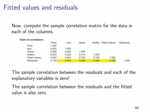
Now, compute the sample correlation matrix for the data ineach of the columns.
Table of correlations
Price size nbeds nbaths Fitted Values Residuals
Price 1.000
size 0.553 1.000
nbeds 0.526 0.484 1.000
nbaths 0.523 0.523 0.415 1.000
Fitted Values 0.663 0.834 0.793 0.789 1.000
Residuals 0.749 0.000 0.000 0.000 0.000 1.000
The sample correlation between the residuals and each of theexplanatory variables is zero!
The sample correlation between the residuals and the fittedvalue is also zero.
50

Fitted values and residuals
1.5 1.6 1.7 1.8 1.9 2.0 2.1 2.2 2.3 2.4 2.5 2.6
-40
-20
0
20
40R
esid
uals
House size
It is always a good idea to plot your residuals. There should beno obvious patterns in them.
51

Fitted values and residuals
Given the above properties we know that we can “split up” yiinto two parts
yi = yi + ei
Just like for simple regression, we ask “how much variation iny can be explained by the x ’s?”
We want to break the total variation of y into two parts.
52

Fitted values and residuals
We have a linear relationship
yi = yi + ei
and consequently we can use our linear formulas to computethe sample mean and variance of y .
The sample variance is
s2y = s2y + s2e
53

Starting with s2y = s2y + s2e , we know that
n∑i=1
(yi − y)2 =n∑
i=1
(yi − y)2 +n∑
i=1
e2i
This is the same as in Lecture # 9. Therefore, we have:
I∑n
i=1 (yi − y)2. This is the total variation in y .
I∑n
i=1 (yi − y)2. This is the variation in y explained by x .This is often called the “explained sum of squares (ESS).”
I∑n
i=1 e2i . This is the unexplained variation in y .
54

Explained and Unexplained Variation
Here is our Excel output.
The explained sum of squares (ESS) is:∑ni=1 (yi − y)2 = 40300.99
The unexplained sum of squares is:∑n
i=1 e2i = 51384.22
55
R-squared
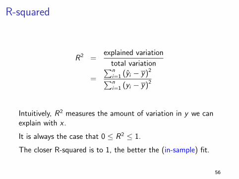
R2 =explained variation
total variation
=
∑ni=1 (yi − y)2∑ni=1 (yi − y)2
Intuitively, R2 measures the amount of variation in y we canexplain with x .
It is always the case that 0 ≤ R2 ≤ 1.
The closer R-squared is to 1, the better the (in-sample) fit.
56

R-squared
Here is our Excel output.
R2 = explained variationtotal variation
= 40300.9940300.99+51384.22
= 0.439
57

R-squared
In a multiple linear regression, R2 is also the correlation squared between
the fitted values yi and the observed values yi .
The correlation is cor(y , y) = 0.663 which gives(0.663)2 = 0.439
58
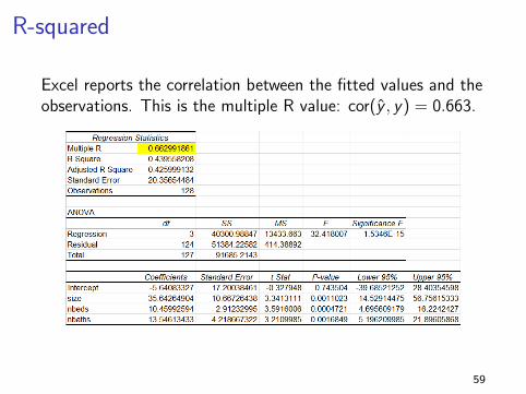
R-squared
Excel reports the correlation between the fitted values and theobservations. This is the multiple R value: cor(y , y) = 0.663.
59
R-squared
Note #3: “What happens to R2 when I add more variables?”
People often misinterpret and/or overemphasize R2. Forexample, I might have different x ’s and not know which x ’s toinclude in a regression.
A first reaction is to run a number of different regressions and“choose the regression with the highest R2.”
WARNING: Be careful! It turns out that when you add moreexplanatory variables R2 will NEVER go down!
In addition, the higher the R2 does not mean that yourpredictions will be better.
60

The overall F -test
61

The overall F -test
Earlier, we discussed how t-stats can be used to examine thenull hypothesis H0 : βj = 0 for each individual coefficient.
However, what if we would like to test the null hypothesis that all the
coefficients are equal to zero? In other words, H0 : β1 = β2 = β3 = 0.
62

The overall F -test
The null hypothesis H0 : β1 = β2 = · · · = βk = 0 can betested using an F -test.
This null hypothesis is a joint hypothesis that all the slopes areequal to zero.
This is called an F -test because the sampling distribution ofthe test statistic is an F -distribution.
The phrase “overall” comes from the fact that we are testingall the slope coefficients and not a subset of them.
63

The overall F -test
Excel automatically prints out the overall F -test as well as thep-value for this test statistic.
We reject the null. This tells us that at least some of the slopes are not 0.
64

The overall F -test
Some people refer to the “overall F -test” as the “kitchen sinktest”. Notice that if the null hypothesis
H0 : β1 = β2 = · · · = βk = 0
is true then none of the x ’s have ANY explanatory power inour linear model!
We’ve thrown “everything but the kitchen sink” at Y . Wewant to know: can ANY of our x ’s predict Y ?
In practice, this test is very sensitive. You’re being “maximallyskeptical” here, so you will usually reject H0.
65
Categorical variables
66

Categorical variables
Here once again are the first 10 rows of our housing data.
Home Nbhd Offers SqFt Brick Bedrooms Bathrooms Price
1 2 2 1790 No 2 2 114300
2 2 3 2030 No 4 2 114200
3 2 1 1740 No 3 2 114800
4 2 3 1980 No 3 2 94700
5 2 3 2130 No 3 3 119800
6 1 2 1780 No 3 2 114600
7 3 3 1830 Yes 3 3 151600
8 3 2 2160 No 4 2 150700
9 2 3 2110 No 4 2 119200
10 2 3 1730 No 3 3 104000
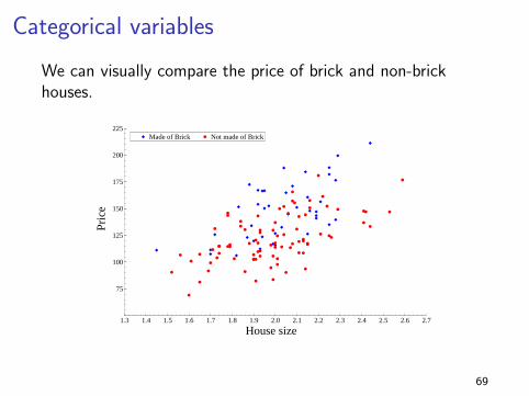
Does whether or not a house is made of brick affect the price?
This is a categorical variable.
Can we use multiple regression when one (or more) of our xvariables is categorical?
67

Categorical variables
We can add an additional column which is a dummy variableto indicate whether a house is made of brick.
Home Nbhd Offers SqFt Brick Bedrooms Bathrooms Price brickdum
1 2 2 1790 No 2 2 114300 0
2 2 3 2030 No 4 2 114200 0
3 2 1 1740 No 3 2 114800 0
4 2 3 1980 No 3 2 94700 0
5 2 3 2130 No 3 3 119800 0
6 1 2 1780 No 3 2 114600 0
7 3 3 1830 Yes 3 3 151600 1
8 3 2 2160 No 4 2 150700 0
9 2 3 2110 No 4 2 119200 0
10 2 3 1730 No 3 3 104000 0
If it is, then we give it a 1 and a 0 otherwise. (In Excel, try
=IF(E2=”YES”,1,0) )
68
Categorical variables
We can visually compare the price of brick and non-brickhouses.
Made of Brick Not made of Brick
1.3 1.4 1.5 1.6 1.7 1.8 1.9 2.0 2.1 2.2 2.3 2.4 2.5 2.6 2.7
75
100
125
150
175
200
225
House size
Pric
e
Made of Brick Not made of Brick
69

Categorical variables
As a simple first example, let’s regress price on size andbrickdum.
Here is our model
Pricei = α + β1sizei + β2brickdumi + εi
Question: How do we interpret β2?
70

Categorical variables
Here is our model
Pricei = α + β1sizei + β2brickdumi + εi
Question: How do we interpret β2?
Answer: β2 is the expected difference in price between a brickand non-brick house controlling for size.
71

Categorical variables
What is the expected price of a brick house given that its sizeis “size = s”?
E[Price|size = s, brickdum = 1] = α + β1s + β2
Our slope is β1 and our intercept is α + β2.
What is the expected price of a non-brick house given that itssize is “size = s”?
E[Price|size = s, brickdum = 0] = α + β1s
Our slope is β1 and our intercept is α.
72

Categorical variables
What this tells us is that we can interpret β2 as a shift in theintercept.
Notice that our model still assumes that the price differencebetween a brick and non-brick house does not depend on thesize!
In other words, we are fitting two lines with different interceptsbut the slopes are still the same.
73

Results
Here are the results of this regression from Excel.
Notice that our estimate of the standard deviation se is smallerthan before so our predictions will improve.
74

Categorical variables
Made of Brick Not made of Brick
1.3 1.4 1.5 1.6 1.7 1.8 1.9 2.0 2.1 2.2 2.3 2.4 2.5 2.6 2.7
75
100
125
150
175
200
225
y = a + b2 + b1size
y = a + b1size
House size
Pric
eMade of Brick Not made of Brick
Here, I have plotted the fitted values yi . In this case, we justfit two lines with different intercepts but the same slope.
75

Dummy variables
Note # 4: “How do I define a dummy variable?”
We could switch the definition of a dummy variable around.We could create a dummy which was 1 if a house was nonbrick and 0 if brick.
That would be fine, but the meaning of β2 would change.
CAUTION: You CANNOT put both dummies variables intothe regression! Given one, the information in the other isredundant.
76

Categorical variables
Here are the Excel results from the larger regression includingnbed and nbath.
77

Categorical variables
We can also create dummy variables from the neighborhoodcategory.
Home Nbhd Offers SqFt Bedrooms Bathrooms Price Nbhd1 Nbhd2 Nbhd3
1 2 2 1790 2 2 114300 0 1 0
2 2 3 2030 4 2 114200 0 1 0
3 2 1 1740 3 2 114800 0 1 0
4 2 3 1980 3 2 94700 0 1 0
5 2 3 2130 3 3 119800 0 1 0
6 1 2 1780 3 2 114600 1 0 0
7 3 3 1830 3 3 151600 0 0 1
8 3 2 2160 4 2 150700 0 0 1
9 2 3 2110 4 2 119200 0 1 0
10 2 3 1730 3 3 104000 0 1 0
For example, the variable nbhd1 indicates whether the houseis in neighborhood #1.
You can include any 2 out of the 3 variables nbhd1, nbhd2,and nbhd3 in the regression.
78
Categorical variables
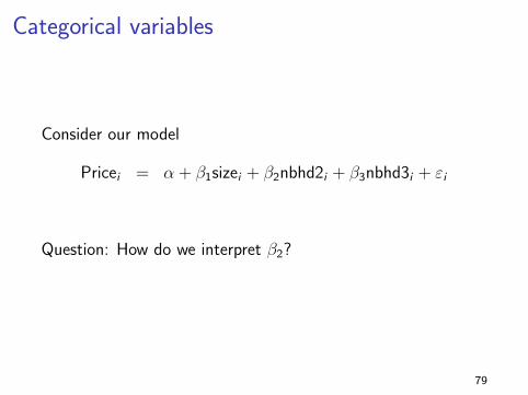
Consider our model
Pricei = α + β1sizei + β2nbhd2i + β3nbhd3i + εi
Question: How do we interpret β2?
79

Categorical variables
Consider our model
Pricei = α + β1sizei + β2nbhd2i + β3nbhd3i + εi
Question: How do we interpret β2?
Answer: β2 is the expected difference in price between a housein neighborhood 2 relative to neighborhood 1.
The neighborhood corresponding to the dummy we leave outbecomes the “base case” we compare to.
80

Categorical variables
What is the expected price of a house given that its size is“size = s” and it is in neighborhood # 1?
E[Price|size = s] = α + β1s
Consider the same house but with “nbhd2 = 1.”
E[Price|size = s] = α + β1s + β2
Consider the same house but with “nbhd3 = 1.”
E[Price|size = s] = α + β1s + β3
81

Categorical variables
Consider one last model
Pricei = α + β1sizei + β2nbedi + β3nbathi
+β4brickdumi + β5nbhd2i + β6nbhd3i + εi
In this case, the interpretation of the regression coefficientsfollows the same line of reasoning.
82

Categorical variables
Here are the Excel results from this regression.
83

Summary: categorical variables
I In general to add a categorical x , you can createdummies, one for each possible category.
I Use all but one of the dummies.
I It does not matter which one you drop for the fit, but theinterpretation of the coefficients will depend on which oneyou choose to drop.
84

Summary: multiple regression
I Multiple linear regression attempts to find a linearcombination of the explanatory variables x that “bestfits” the data y .
I We interpret the fitted values y as the part of y explainedby the x ’s.
I The residuals ei are the part of y unexplained by the x ′s.
I To interpret the estimates βj for j = 1, . . . , k , we considerwhat happens to y for a one unit change in x·,j with allthe other explanatory variables held fixed.
85

Other topics in multiple regression
If you choose to take a regression class, you will go throughthe math in more detail and you will cover additional topics
I model selection: Which variables x should I put in myregression?
I heteroskedasticity: What happens when the variance σ2
is not constant for all observations?
I omitted variables: Sometimes there is a variable thatwe would like to have as one of our x ’s but we do notobserve it.
I nonlinearities: Sometimes y may be better explained bya nonlinear function of x .
I outliers: Sometimes there are a few observations that areaberrant. These can highly influence our results.
86


![The lipogenic transcription factor ChREBP dissociates ...dm5migu4zj3pb.cloudfront.net/manuscripts/41000/... · [MUFAs]) were preferentially enriched. Lastly, we measured the expression](https://img.pdfslide.us/doc/110x75/5ec0b2578499721e41710b35/the-lipogenic-transcription-factor-chrebp-dissociates-mufas-were-preferentially.jpg)