BUSINESS MATHEMATICS

&

STATISTICS

LECTURE 45Planning Production Levels: Linear Programming

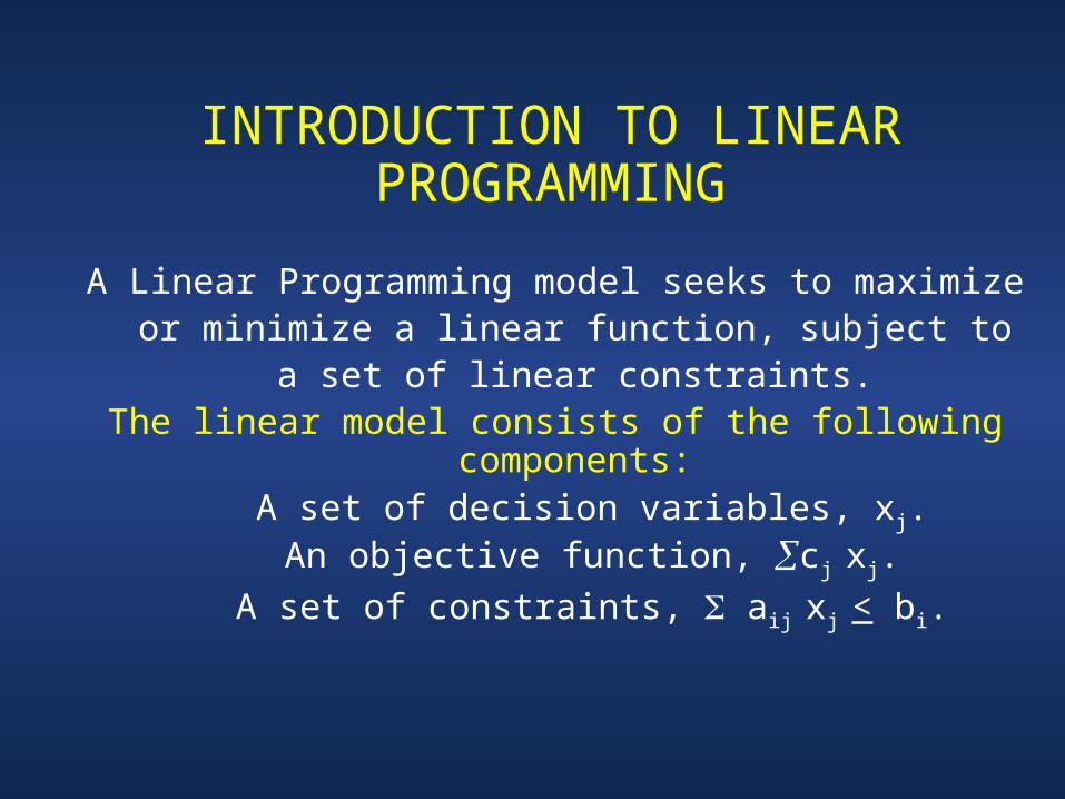
A Linear Programming model seeks to maximize or minimize a linear function, subject to a set of linear

constraints.The linear model consists of the following

components: A set of decision variables, xj. An objective function, cj xj.

A set of constraints, aij xj < bi.

INTRODUCTION TO LINEAR PROGRAMMING

THE FORMAT FOR AN LP MODEL

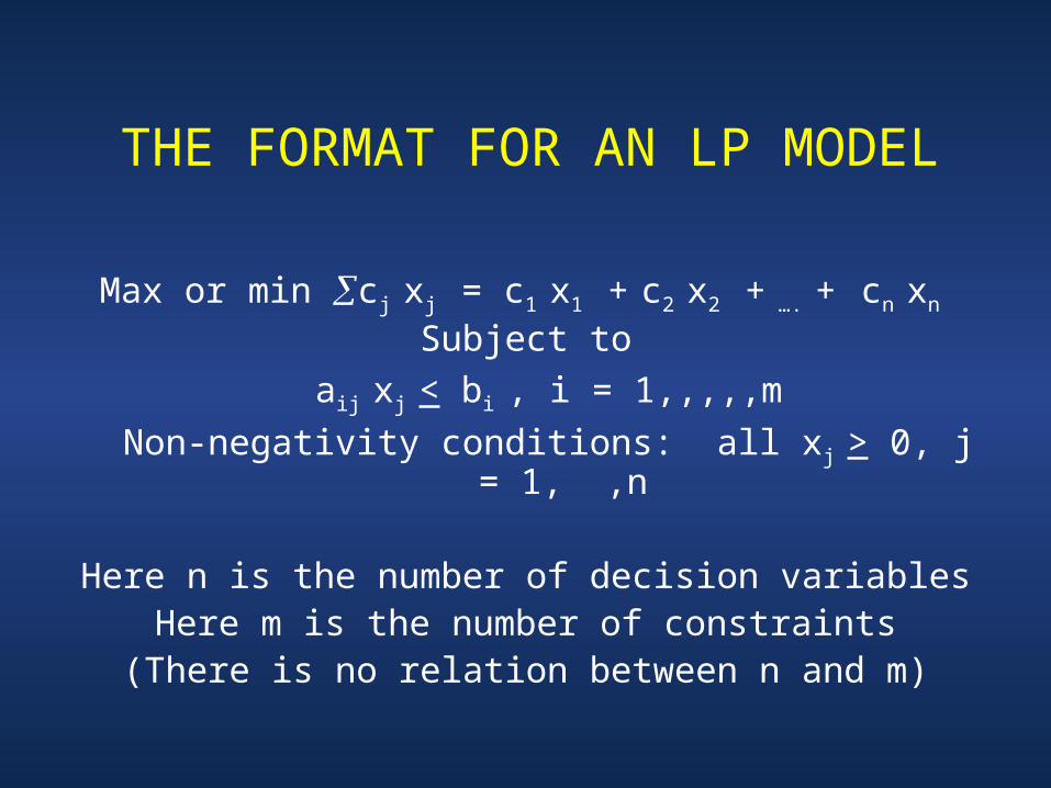
Max or min cj xj = c1 x1 + c2 x2 + …. + cn xn

Subject to

aij xj < bi , i = 1,,,,,m

Non-negativity conditions: all xj > 0, j = 1, ,n

Here n is the number of decision variablesHere m is the number of constraints

(There is no relation between n and m)

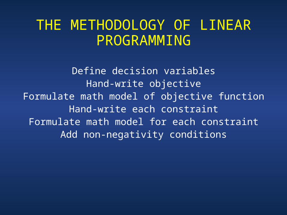
THE METHODOLOGY OF LINEAR PROGRAMMING

Define decision variablesHand-write objective

Formulate math model of objective functionHand-write each constraint

Formulate math model for each constraintAdd non-negativity conditions

Introduction to Linear Programming

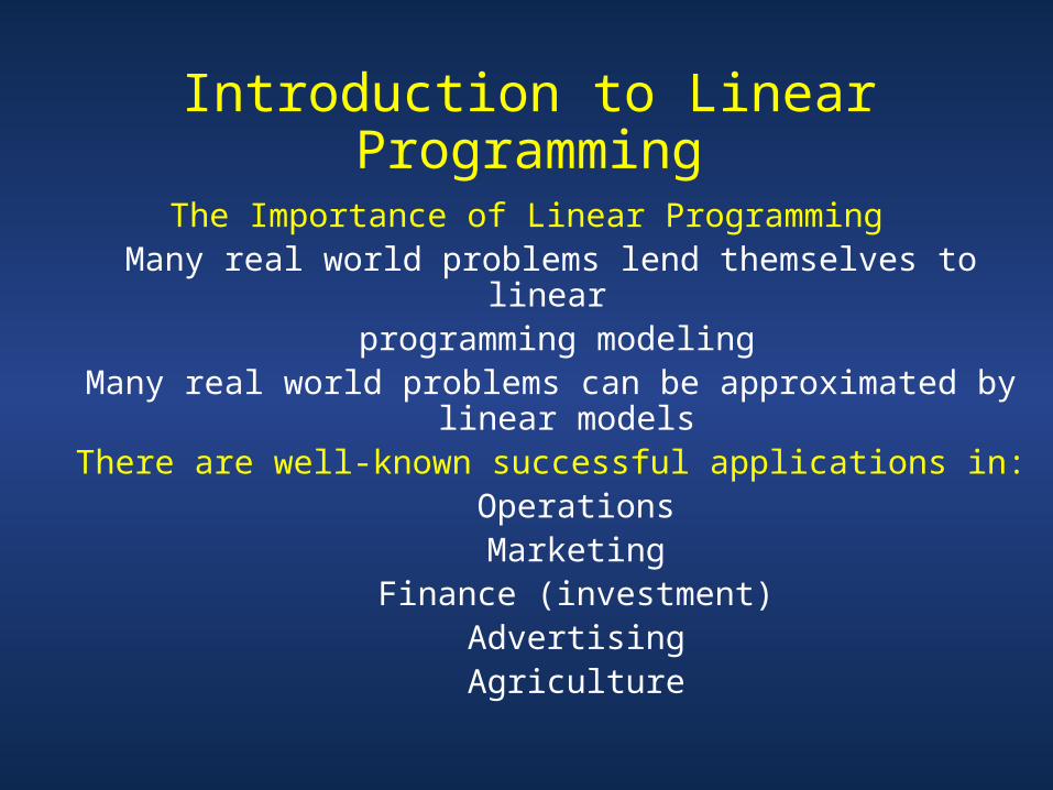
The Importance of Linear ProgrammingMany real world problems lend themselves to linear

programming modeling Many real world problems can be approximated by linear

modelsThere are well-known successful applications in:

OperationsMarketing

Finance (investment)AdvertisingAgriculture

The Importance of Linear Programming

There are efficient solution techniques that solve linear programming models

The output generated from linear programming packages provides useful “what if” analysis

Introduction to Linear Programming

Introduction to Linear Programming

Assumptions of the linear programming model

The parameter values are known with certainty

The objective function and constraints exhibit constant returns to scale

There are no interactions between the decision variables (the additivity assumption)

The Continuity assumption: Variables can take on any value within a given feasible range

A Production Problem – A Prototype Example

A company manufactures two toy doll models:

Doll A

Doll B

Resources are limited to

1000 kg of special plastic

40 hours of production time per week

Marketing requirement

Total production cannot exceed 700 dozens

Number of dozens of Model A cannot exceed number

of dozens of Model B by more than 350

Technological inputModel A requires 2 kg of plastic and

3 minutes of labour per dozen.

Model B requires 1 kg of plastic and

4 minutes of labour per dozen

A Production Problem – A Prototype Example

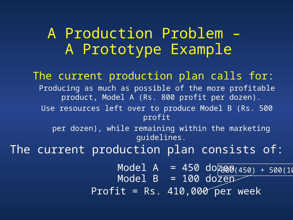
The current production plan calls for: Producing as much as possible of the more profitable product,

Model A (Rs. 800 profit per dozen).

Use resources left over to produce Model B (Rs. 500 profit

per dozen), while remaining within the marketing guidelines.

The current production plan consists of:

Model A = 450 dozenModel B = 100 dozen

Profit = Rs. 410,000 per week

A Production Problem – A Prototype Example

800(450) + 500(100)

A Production Problem – A Prototype Example

Management is seeking

a production schedule

that will increase

the company’s profit

A Production Problem – A Prototype Example

A linear programming model can providean insight

and an intelligent solution

to this problem

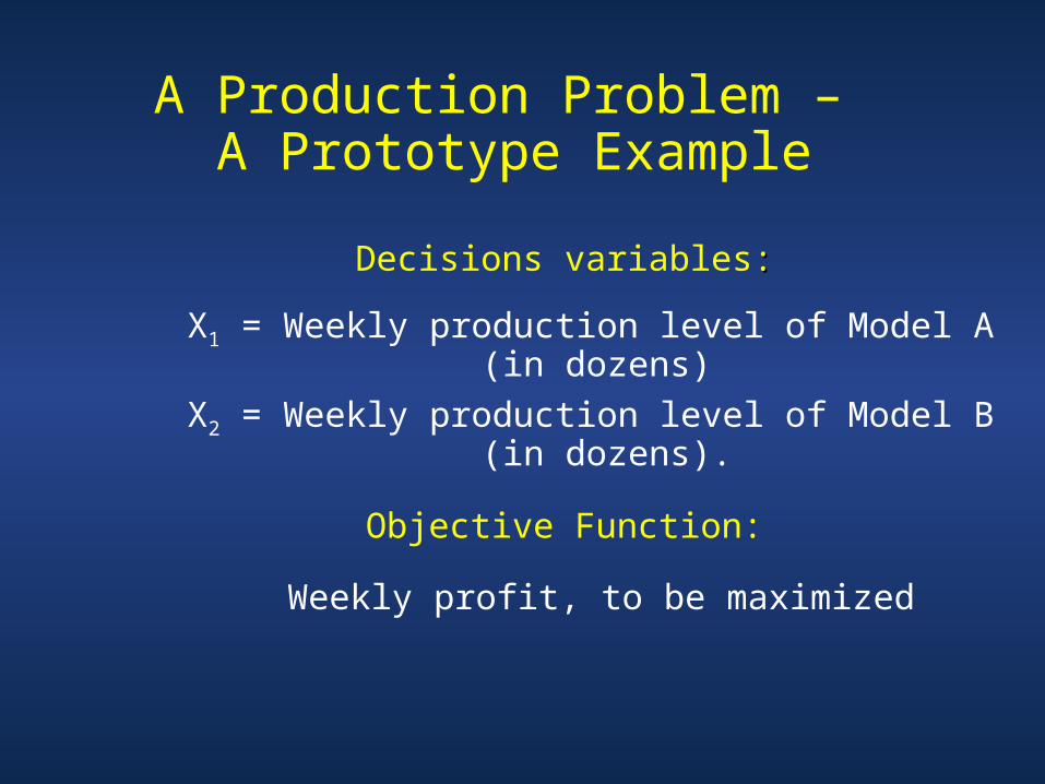
Decisions variables::

X1 = Weekly production level of Model A (in dozens)

X2 = Weekly production level of Model B (in dozens).

Objective Function:

Weekly profit, to be maximized

A Production Problem – A Prototype Example

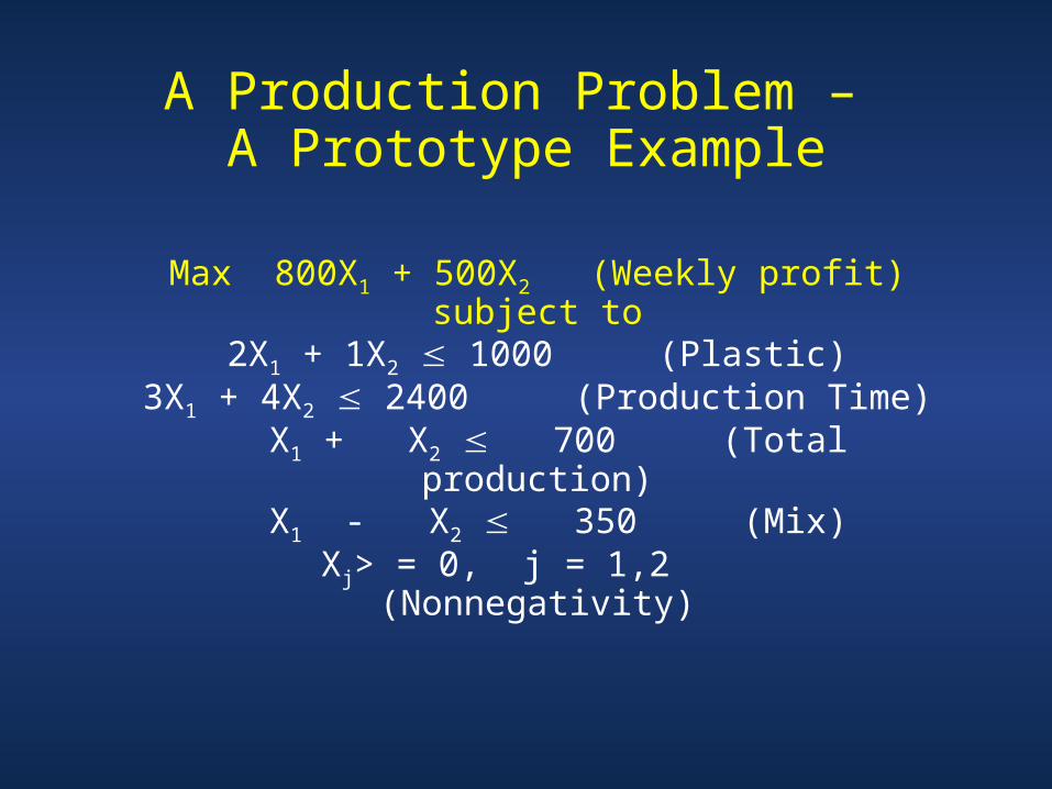
Max 800X1 + 500X2 (Weekly profit)subject to

2X1 + 1X2 1000 (Plastic)3X1 + 4X2 2400 (Production Time) X1 + X2 700 (Total production)

X1 - X2 350 (Mix) Xj> = 0, j = 1,2 (Nonnegativity)

A Production Problem – A Prototype Example

ANOTHER EXAMPLE

A dentist is faced with deciding: how best to split his practice

between the two services he offers—general dentistry and pedodontics

(children’s dental care) Given his resources,

how much of each service should he provide to maximize his profits?

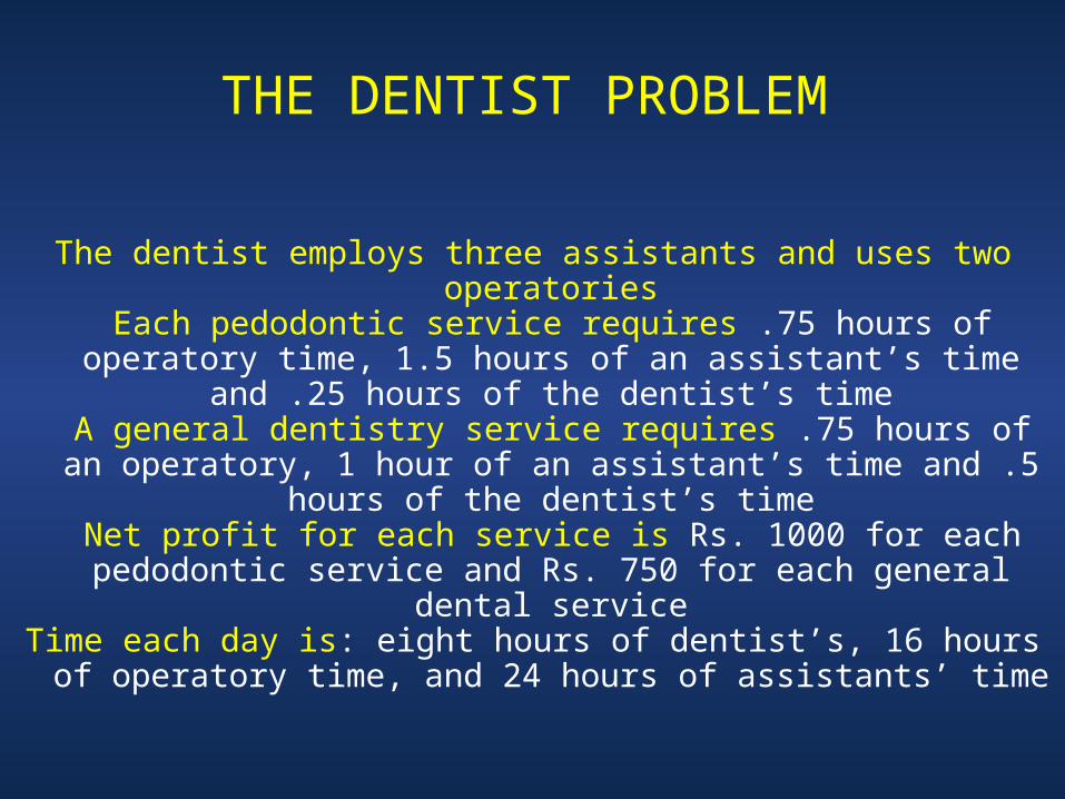
THE DENTIST PROBLEM

The dentist employs three assistants and uses two operatories Each pedodontic service requires .75 hours of operatory time,

1.5 hours of an assistant’s time and .25 hours of the dentist’s time

A general dentistry service requires .75 hours of an operatory, 1 hour of an assistant’s time and .5 hours of the dentist’s time

Net profit for each service is Rs. 1000 for each pedodontic service and Rs. 750 for each general dental service

Time each day is: eight hours of dentist’s, 16 hours of operatory time, and 24 hours of assistants’ time

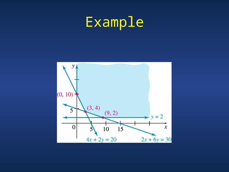
The Graphical Analysis of Linear Programming

The set of all points that satisfy

all the constraints of the model is called a

FEASIBLE REGIONFEASIBLE REGION

THE GRAPHICAL ANALYSIS OF LINEAR PROGRAMMING

Using a graphical presentation we can represent all the constraints,

the objective function, and

the three types of feasible points

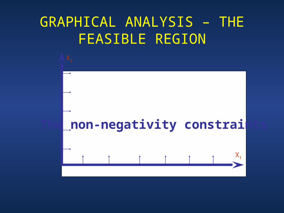
The non-negativity constraints

X2

X1

GRAPHICAL ANALYSIS – THE FEASIBLE REGION

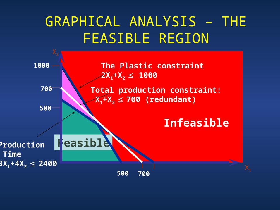
1000

500

Feasible

X2

Infeasible

Production Time3X1+4X2 2400

Total production constraint: X1+X2 700 (redundant)

500

700

The Plastic constraint2X1+X2 1000

X1

700

GRAPHICAL ANALYSIS – THE FEASIBLE REGION

1000

500

Feasible

X2

Infeasible

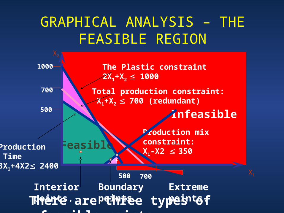
Production Time3X1+4X22400

Total production constraint: X1+X2 700 (redundant)

500

700

Production mix constraint:X1-X2 350

The Plastic constraint2X1+X2 1000

X1

700

GRAPHICAL ANALYSIS – THE FEASIBLE REGION

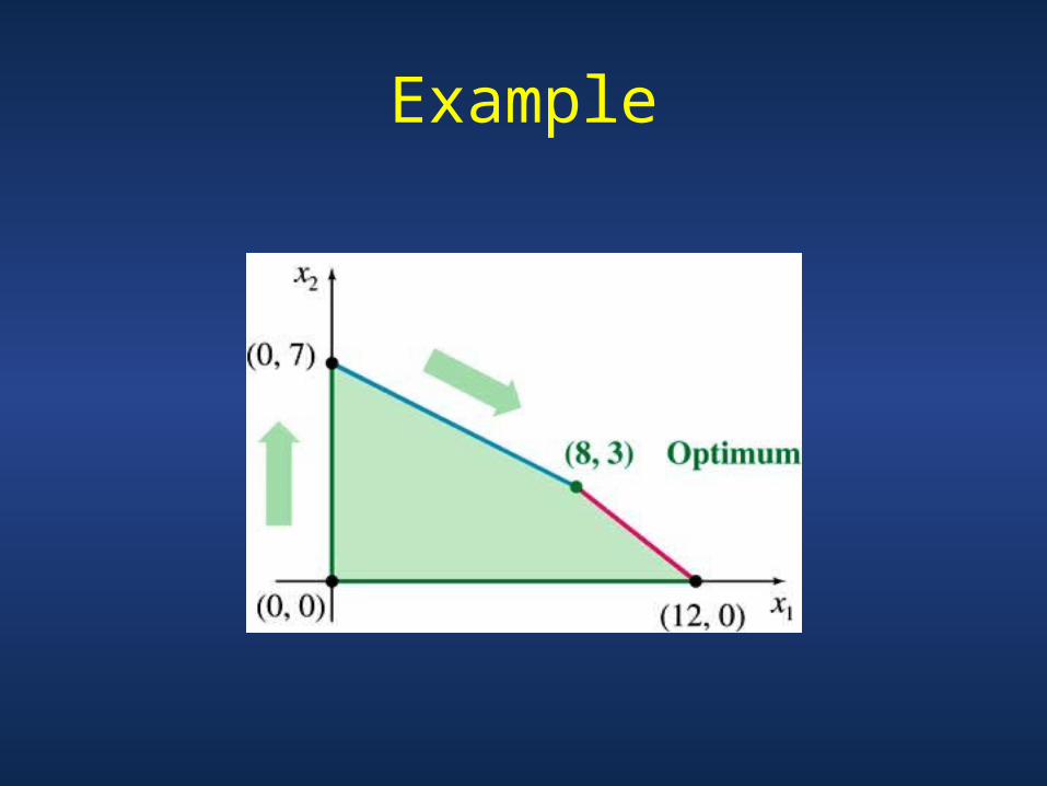
There are three types of feasible pointsInterior points. Boundary points. Extreme points.

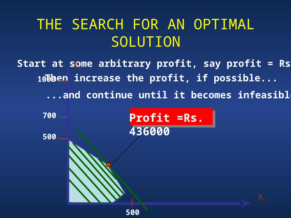
THE SEARCH FOR AN OPTIMAL SOLUTION

Start at some arbitrary profit, say profit = Rs.200,000...

Then increase the profit, if possible...

...and continue until it becomes infeasible

Profit =Rs. 436000

500

700

1000

500

X2

X1

SUMMARY OF THE OPTIMAL SOLUTION

Model A = 320 dozenModel B = 360 dozenProfit = Rs. 436000

This solution utilizes all the plastic and all the production hours

Total production is only 680 (not 700)Model a production does not exceed Model B production at

all

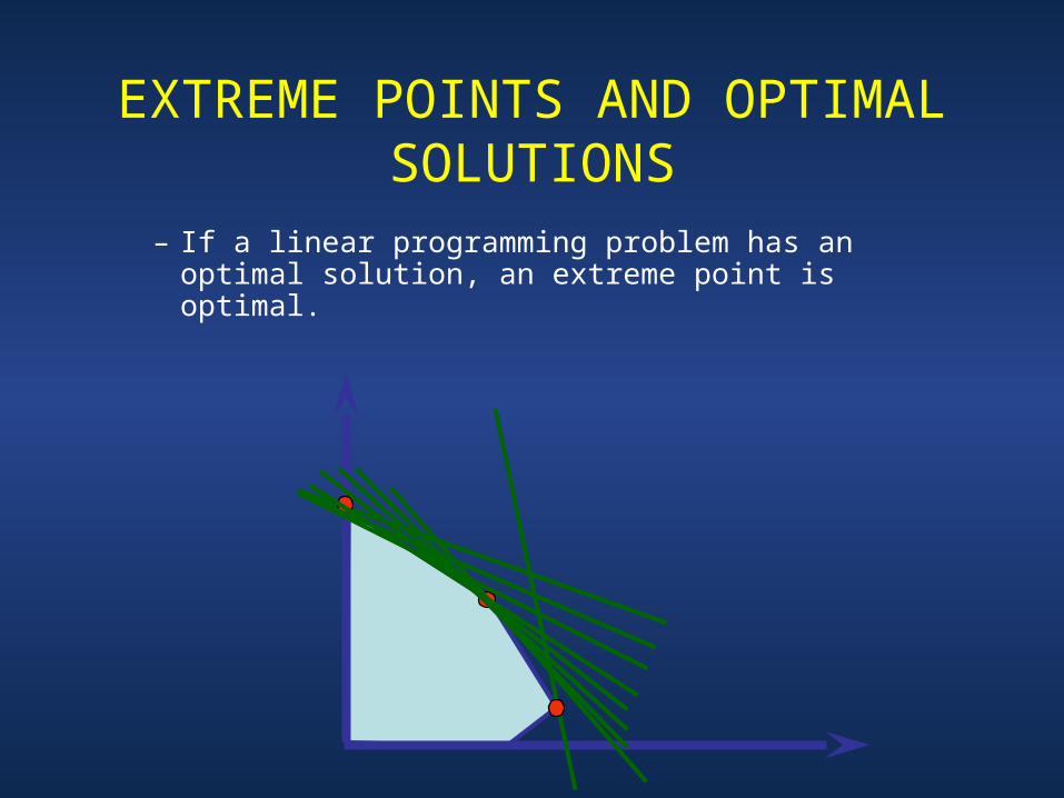
– If a linear programming problem has an optimal solution, an extreme point is optimal.

EXTREME POINTS AND OPTIMAL SOLUTIONS

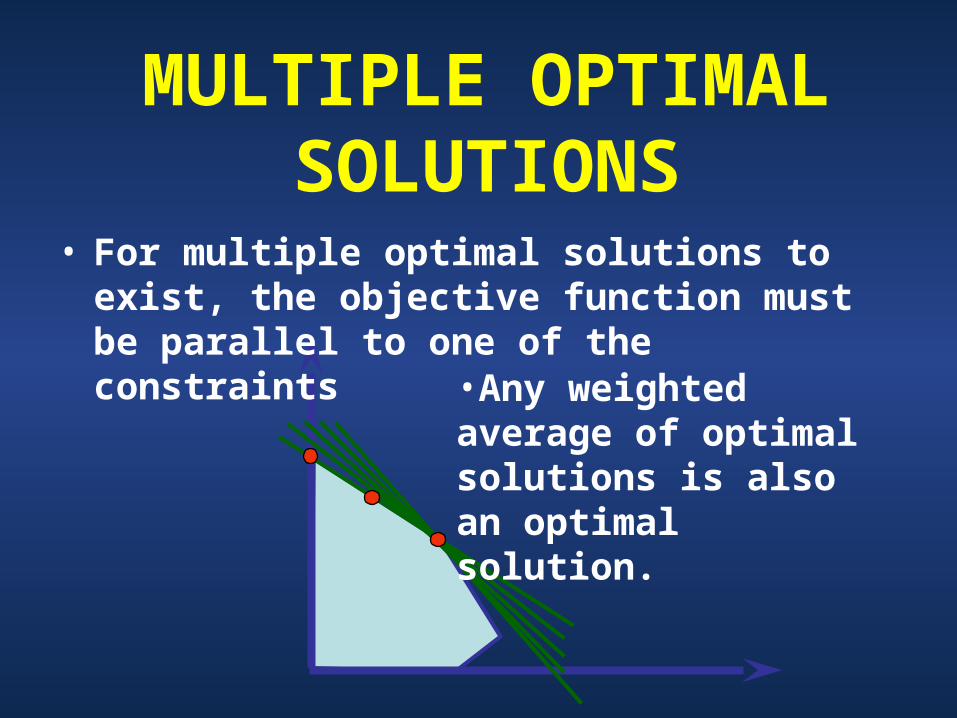
• For multiple optimal solutions to exist, the objective function must be parallel to one of the constraints

MULTIPLE OPTIMAL SOLUTIONS

•Any weighted average of optimal solutions is also an optimal solution.

BUSINESS MATHEMATICS

&

STATISTICS

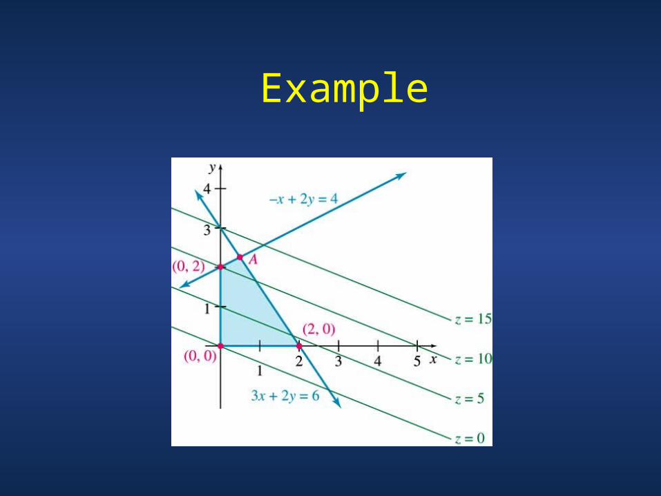
Example

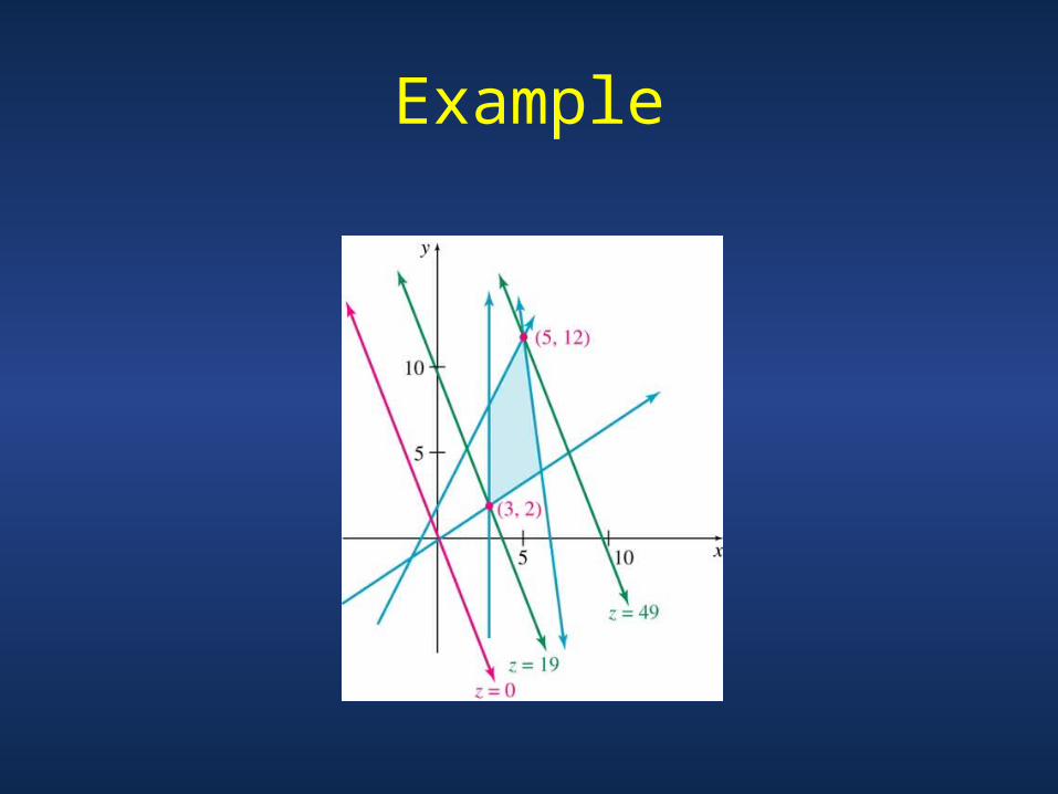
Example

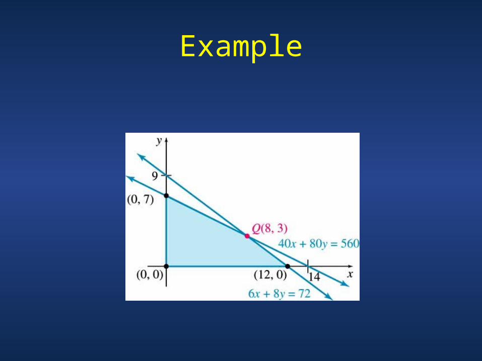
Example

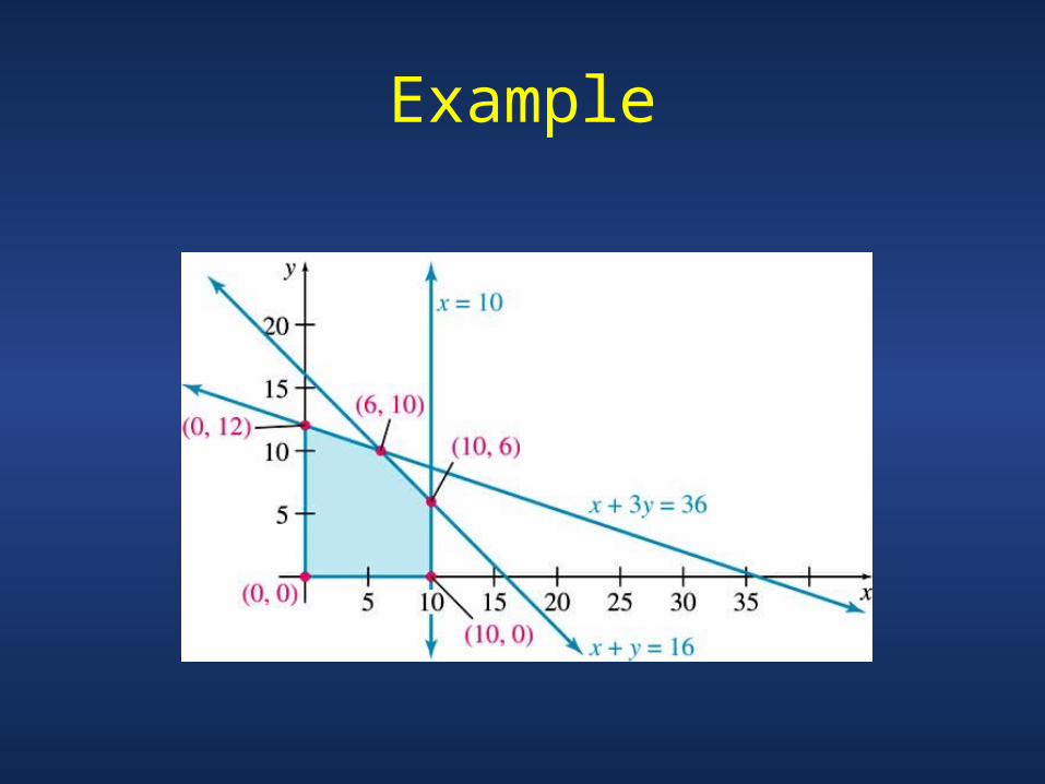
Example

Example

Example