Embed Size (px)
Citation preview

Business Intelligence
• Data Warehouse drives the corporate information supply chain to support Corporate Business Intelligence process.
• Business Intelligence introduced by Howard Dresner of the Gartner Group in 1989 is a set of concepts and methodologies to improve decision-making in business through the use of facts and fact-based systems.
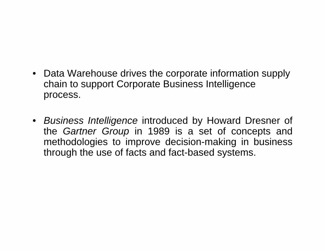
Fact-Based Systems
• Executive Information Systems• Decision Support Systems• Enterprise Information Systems• Management Support Systems• OLAP• Data & Text Mining• Data Visualization• Geographic Information Systems
Data Warehousing
• This simple concept has recently become a Multi-Billion dollar industry.
• New Breeds of vendors are introducing tools and technologies at an alarming rate to deliver data warehouse solutions.
• This fast-paced and fluid data warehousing industry makes it difficult to select a set of technologies to implement a Data warehouse.
• That will stay in the data warehousing industry in the coming years.
The Construction of a Data Warehouse requires three key
steps:
– Extract data from transactions systems.– Manipulate extracted data to generate
reports.– Makes such reports accessible to the
decision-makers.
Data Warehouse Categories• Terms Used to define data warehouse objects vary from
one vendor to another and can be divided into the following categories.
• Data Warehouse.• Data Mart.• Operational Data Store.• Extraprise Data Warehouse.
First Chapter
• What is Data Warehousing? • Data Warehousing Architecture• Components of Data Warehousing• Evolution of ERP Data Warehousing• A Multi-Dimensional Data model
Data Warehouse.
• This is conceptually the same defined my Inmon.
• It could be one large physical instance or a collection of several physical data object instances (Detailed & Aggregated), each serving a special purpose conforming to a grander corporate vision.
Data Mart• Data Marts are stand-alone small data
warehouses limited to a subject area (Ex:- Sales Analysis).
• We have Dependent and Independent data marts.
• Dependent Data Marts are extracted views of a corporate data warehouse.
• Independent Data Marts are those which are built directly against transaction systems.
Operational Data Store• The operational data store is a central data repository that
consists of very detailed level transaction data.
• * * Data warehouses and Data Marts are built by fetching data from ODS instead of transaction systems.
• Moreover , ODS is a Data Consolidation and integration point for several transaction systems.
• More detailed Data may not necessarily needed by data warehousing for analytical purpose.
• ODS Becomes hub for both Data Warehouses & Transaction Systems.
Extraprise Data Warehouse• Extraprise data warehousing are the future
trend in data warehousing.
• Such Data Warehouses , along with typical Decision Support Operations, become an integral component of Enterprise-Business-Critical applications , such as Order administration, Order fulfillment, Customer Relationship Management- across the globe, as well as meet Business-to-Business and Business-to-Consumer information needs.
Data Warehouse Architecture• Building a House is analogous to building a Data
Warehouse.
• The architect draws up a blueprint based on your needs and requirements.
• During design process, the architect makes sure that your living requirements are met.
• If the house does not adhere to an architectural plan, its integrity will always be in question.
SAP BW
• The SAP Business Information Warehouse (SAP BW) follows this paradigm.
• Under one frame work , you can have a huge Extraprise Data warehouse of a hierarchy of enterprise data warehouses or data marts, all conforming to the same architecture, infrastructure and information delivery methods.
What is SAP Business Information Warehouse?
• Today's decision makers urgently need accurate information - a complete and up-to-date picture of their business and their business environment.
• However, that information is spread over a wide variety of platforms and applications throughout the corporate IT structures.
• This can make obtaining vital facts and figures a complex and time-consuming task.
• SAP® Business Information Warehouse (SAP BW) is a robust and scalable data warehouse and forms the foundation of the SAP Business Intelligence (SAP BI) solution.
• The reporting and analysis tools within SAP BW offer a quick andeasy way to gain access to the information you need. SAP BI warehouse management tools let you integrate and store data fromsources throughout the organization and beyond - sources that contribute to strategic analysis and decision making.
Components of Data Warehouse
• Inmon, Ralph Kimball, and Doug Hackney have published several books articulating traditional data warehouse architectures and construction processes.
• Following are the critical layers that are important in understanding the SAP BW architecture.
– Data Provider.– Service Provider.– Information Consumer.– Data Warehouse Management.
Data Provider Layer• The Data provider layer is the primary gateway to the data
sources (OLTP Applications).
• Major tasks performed at this layer provide an environment in which to construct subject-oriented data analysis models.
• Metadata (data about the data) is pulled into a data warehouse environment from its data sources.
• Extraction, Transformation, & Transport services fetch data from data sources , Qualify , perform value- added data manipulation, and push data out to data warehouse data objects.
Data Provider Layer
• Key services performed at this level is – Data Transport.– Data Transformation.– Data cleansing.– Data Extraction.– Subject Models.
Service Provider Layer• The Service Provider Layer is responsible for managing
and distributing data objects across the enterprise to support business intelligence activities in a controlled and secured fashion.
• At this layer, data is further transformed for specific data analysis tasks such as drill-down analysis and predefined reports integration with third-party subscribed data.
• This Layer is very complex within the data warehouse architecture. Key services performed at this layer are the following:
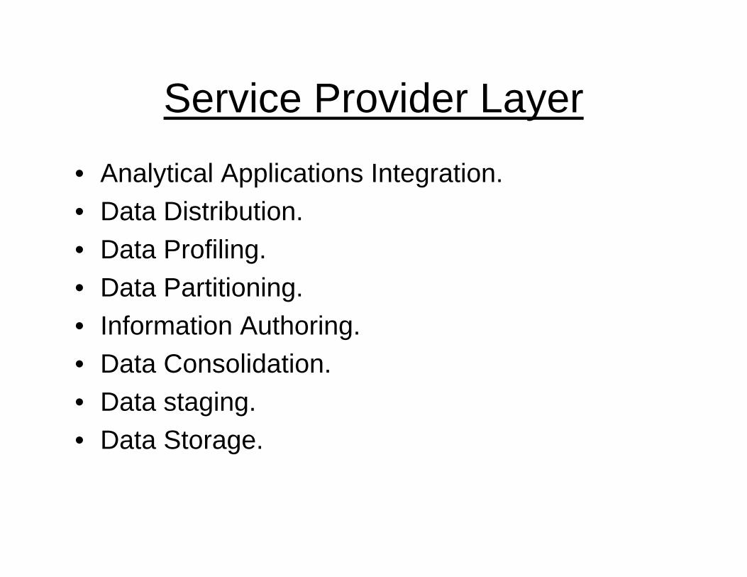
Service Provider Layer
• Analytical Applications Integration.• Data Distribution.• Data Profiling.• Data Partitioning.• Information Authoring. • Data Consolidation.• Data staging.• Data Storage.
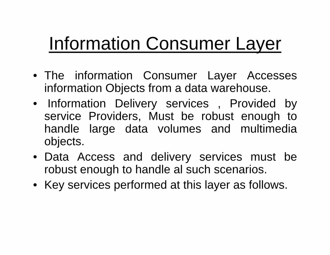
Information Consumer Layer• The information Consumer Layer Accesses
information Objects from a data warehouse.• Information Delivery services , Provided by
service Providers, Must be robust enough to handle large data volumes and multimedia objects.
• Data Access and delivery services must be robust enough to handle al such scenarios.
• Key services performed at this layer as follows.
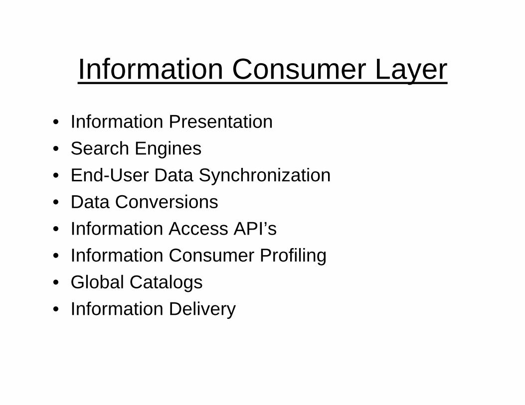
Information Consumer Layer
• Information Presentation• Search Engines• End-User Data Synchronization• Data Conversions• Information Access API’s• Information Consumer Profiling• Global Catalogs• Information Delivery
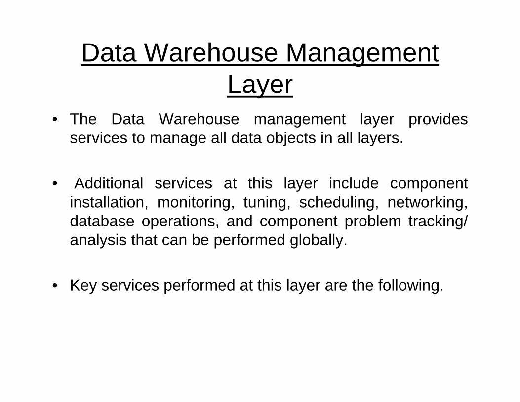
Data Warehouse Management Layer
• The Data Warehouse management layer provides services to manage all data objects in all layers.
• Additional services at this layer include component installation, monitoring, tuning, scheduling, networking, database operations, and component problem tracking/ analysis that can be performed globally.
• Key services performed at this layer are the following.
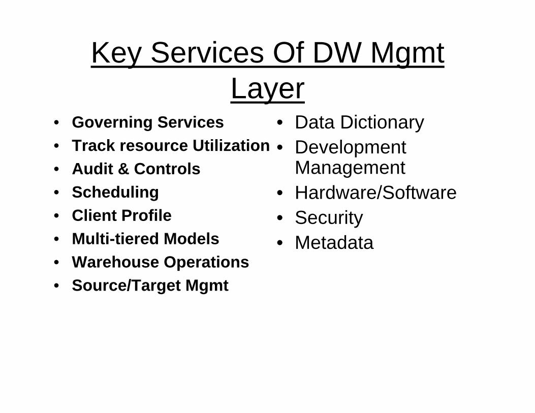
Key Services Of DW Mgmt Layer
• Governing Services• Track resource Utilization• Audit & Controls• Scheduling• Client Profile• Multi-tiered Models• Warehouse Operations• Source/Target Mgmt
• Data Dictionary• Development
Management• Hardware/Software• Security• Metadata

End Of Intro
Definition Data Warehouse
• Defined in many different ways, but not rigorously.– A decision support database that is
maintained separately from the organization’s operational database
– Support information processing by providing a solid platform of consolidated, historical data for analysis.
W.H.Inmon’s Definition
• “A data warehouse is a time-variant, integrated, nonvolatile , &subject-oriented collection of data in support of management’s decision-making process.”—William.H.Inmon - Father of Data Warehousing
Time Variant
• The time horizon for the data warehouse is significantly longer than that of operational systems.– Operational database: current value data.
– Data warehouse data: provide information from a historical perspective (e.g., past 5-10 years)
• Every key structure in the data warehouse– Contains an element of time, explicitly or implicitly
– But the key of operational data may or may not contain “time element”.
Integrated• Constructed by integrating multiple,
heterogeneous data sources– Relational databases, flat files, on-line transaction
records• Data cleaning and data integration techniques
are applied.– Ensure consistency in naming conventions, encoding
structures, attribute measures, etc. among different data sources
• E.g., Hotel price: currency, tax, breakfast covered, etc.– When data is moved to the warehouse, it is
converted.
Non-Volatile
• A physically separate store of data transformed from the operational environment.
• Operational update of data does not occur in the data warehouse environment.– Does not require transaction processing, recovery, and
concurrency control mechanisms
– Requires only two operations in data accessing:
• initial loading of data and access of data.
Subject-Oriented
• Organized around major subjects, such as customer, product, sales.
• Focusing on the modeling and analysis of data for decision makers, not on daily operations or transaction processing.
• Provide a simple and concise view around particular subject issues by excluding data that are not useful in the decision support process.
• Data warehouse: update-driven, high performance– Information from heterogeneous sources is integrated
in advance and stored in warehouses for direct query and analysis
Data Warehouse vs. Operational DBMS
• OLTP (on-line transaction processing)– Major task of traditional relational DBMS– Day-to-day operations: purchasing, inventory,
banking, manufacturing, payroll, registration, accounting, etc.
• OLAP (on-line analytical processing)– Major task of data warehouse system– Data analysis and decision making
OLTP Vs. OLAP• Distinct features (OLTP vs. OLAP):
– User and system orientation: customer Vs. market– Data contents: Current, Detailed Vs. Historical,
Consolidated– Database design: ER + Application Vs. Star + Subject– View: Current, Local Vs. Evolutionary, Integrated– Access patterns: Update vs. Read-only but Complex
Queries
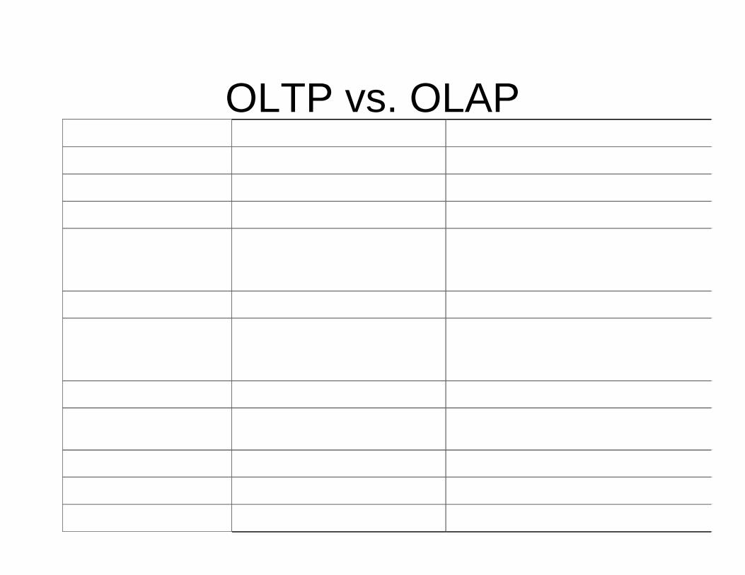
OLTP vs. OLAP OLTP OLAP
Users Clerk, IT Professional Knowledge Worker
Function Day To Day Operations Decision Support
DB design Application-Oriented Subject-Oriented
Data Current, Up-To-Date Detailed, Flat Relational Isolated
Historical, Summarized, Multidimensional Integrated, Consolidated
Usage Repetitive Ad-Hoc
Access Read / Write Index / Hash On Prim. Key
Lots Of Scans
Unit of work Short, Simple Transaction Complex Query
# Records accessed
Tens Millions
# Users Thousands Hundreds
DB size 100mb-Gb 100GB-TB
Metric Transaction Throughput Query Throughput, Response
Tuning for OLTP & OLAP
• High performance for both systems
– DBMS— tuned for OLTP: access methods, indexing, concurrency control, recovery.
– Data Warehouse—tuned for OLAP: complex OLAP queries, multidimensional view, consolidation.
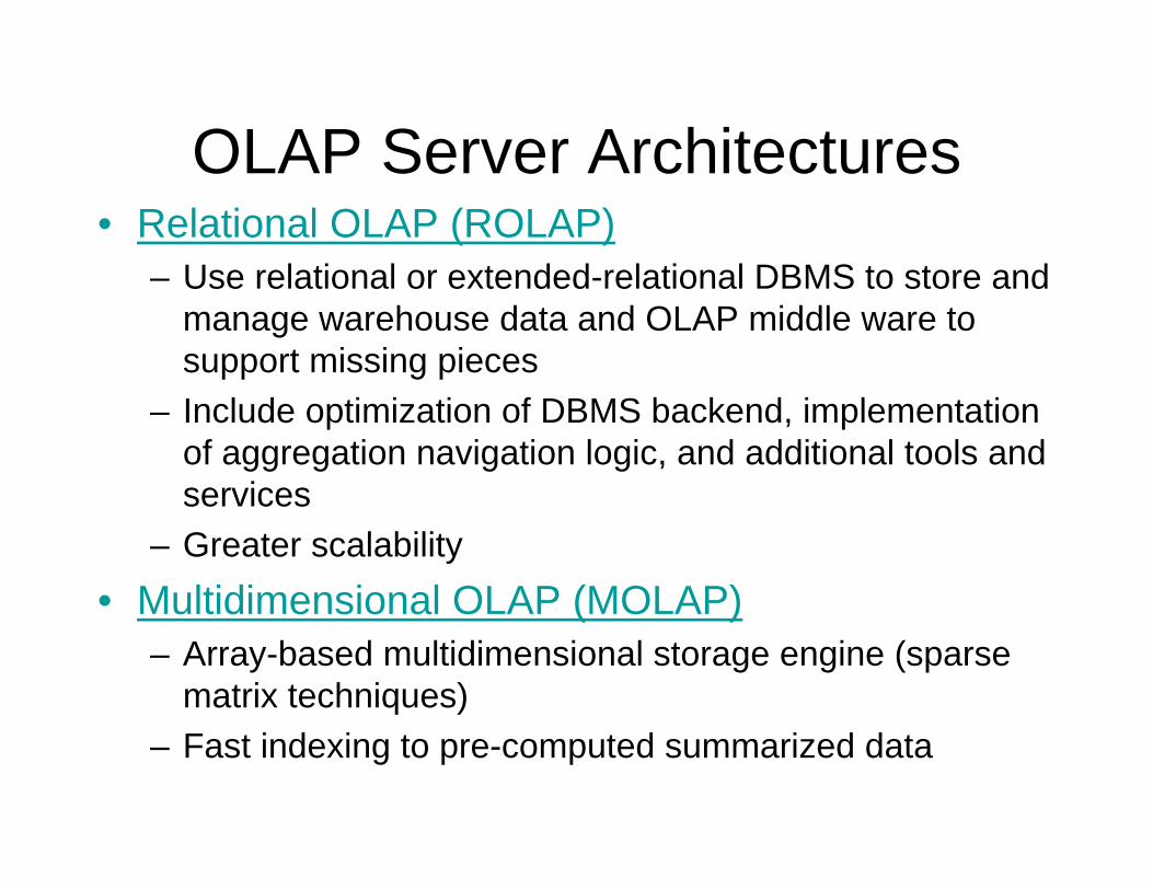
OLAP Server Architectures• Relational OLAP (ROLAP)
– Use relational or extended-relational DBMS to store and manage warehouse data and OLAP middle ware to support missing pieces
– Include optimization of DBMS backend, implementation of aggregation navigation logic, and additional tools and services
– Greater scalability• Multidimensional OLAP (MOLAP)
– Array-based multidimensional storage engine (sparse matrix techniques)
– Fast indexing to pre-computed summarized data
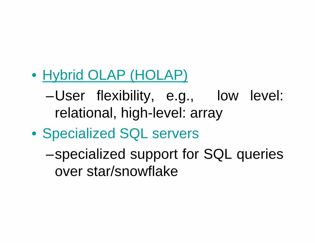
• Hybrid OLAP (HOLAP)–User flexibility, e.g., low level:
relational, high-level: array• Specialized SQL servers
–specialized support for SQL queries over star/snowflake
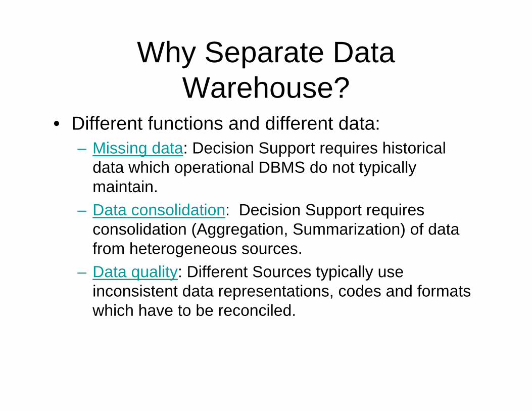
Why Separate Data Warehouse?
• Different functions and different data:– Missing data: Decision Support requires historical
data which operational DBMS do not typically maintain.
– Data consolidation: Decision Support requires consolidation (Aggregation, Summarization) of data from heterogeneous sources.
– Data quality: Different Sources typically use inconsistent data representations, codes and formats which have to be reconciled.

A Multi-Dimensional Data Model
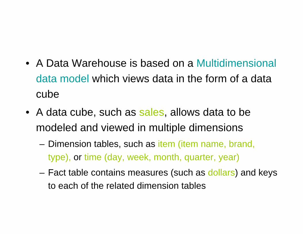
• A Data Warehouse is based on a Multidimensional data model which views data in the form of a data cube
• A data cube, such as sales, allows data to be modeled and viewed in multiple dimensions– Dimension tables, such as item (item name, brand,
type), or time (day, week, month, quarter, year)
– Fact table contains measures (such as dollars) and keys to each of the related dimension tables
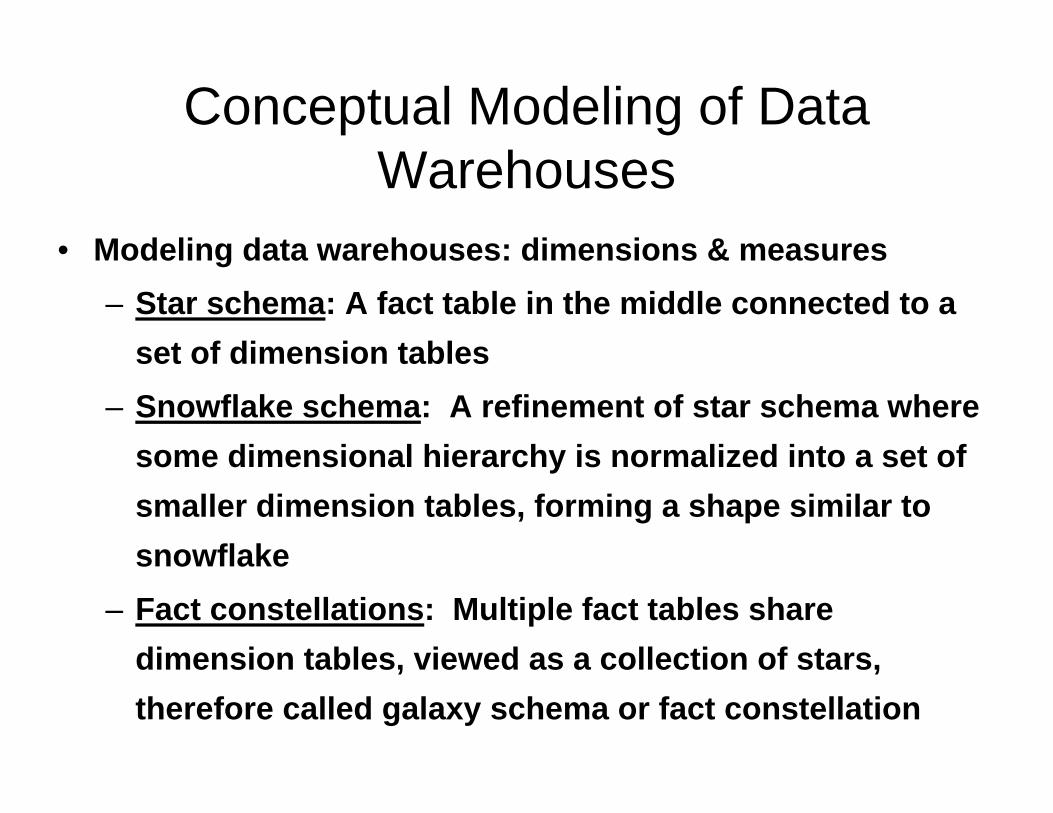
Conceptual Modeling of Data Warehouses
• Modeling data warehouses: dimensions & measures– Star schema: A fact table in the middle connected to a
set of dimension tables – Snowflake schema: A refinement of star schema where
some dimensional hierarchy is normalized into a set of smaller dimension tables, forming a shape similar to snowflake
– Fact constellations: Multiple fact tables share dimension tables, viewed as a collection of stars, therefore called galaxy schema or fact constellation
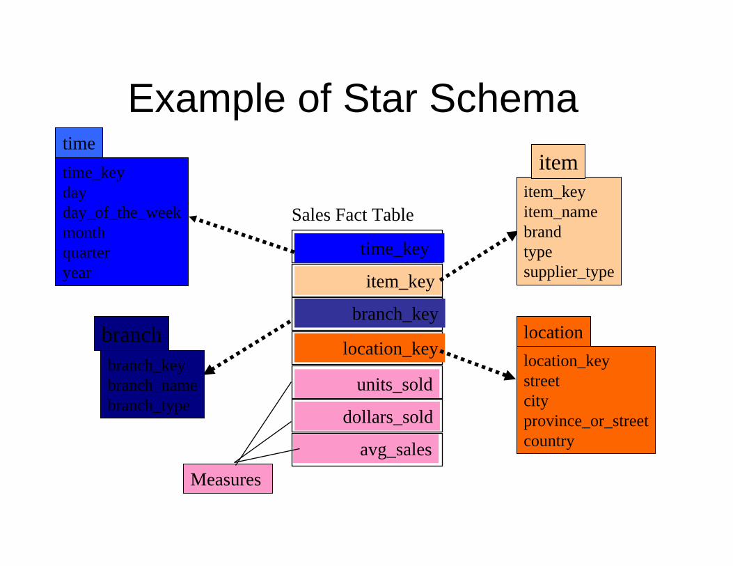
Example of Star Schematime_keydayday_of_the_weekmonthquarteryear
time
location_keystreetcityprovince_or_streetcountry
location
Sales Fact Table
time_key
item_key
branch_key
location_key
units_sold
dollars_sold
avg_salesMeasures
item_keyitem_namebrandtypesupplier_type
item
branch_keybranch_namebranch_type
branch
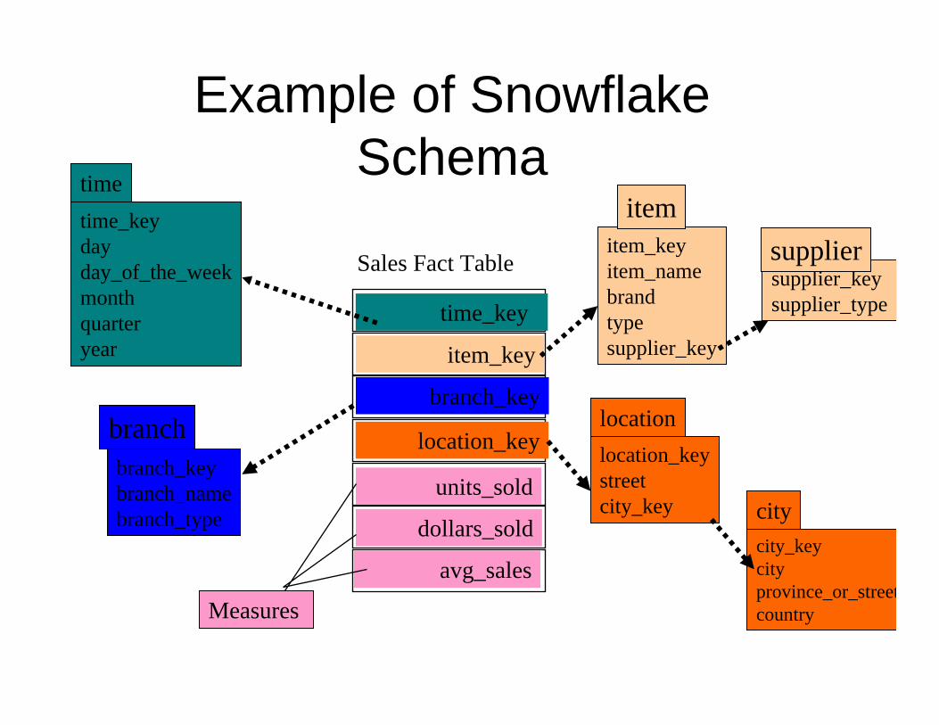
Example of Snowflake Schema
time_keydayday_of_the_weekmonthquarteryear
time
location_keystreetcity_key
location
Sales Fact Table
time_key
item_key
branch_key
location_key
units_sold
dollars_sold
avg_sales
Measures
item_keyitem_namebrandtypesupplier_key
item
branch_keybranch_namebranch_type
branch
supplier_keysupplier_type
supplier
city_keycityprovince_or_streetcountry
city
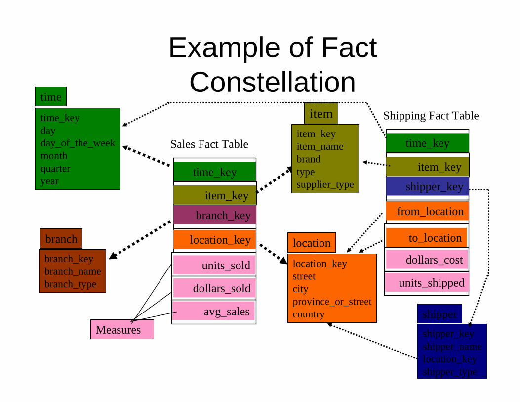
Example of Fact Constellation
time_keydayday_of_the_weekmonthquarteryear
time
location_keystreetcityprovince_or_streetcountry
location
Sales Fact Table
time_key
item_key
branch_key
location_key
units_sold
dollars_sold
avg_salesMeasures
item_keyitem_namebrandtypesupplier_type
item
branch_keybranch_namebranch_type
branch
Shipping Fact Table
time_key
item_key
shipper_key
from_location
to_location
dollars_cost
units_shipped
shipper_keyshipper_namelocation_keyshipper_type
shipper
The Classic Star Schema• Multi-dimensional data models are needed for the creation
of data warehousing or OLAP application, in other words, for analytical applications.
• The classic star schema, is the most frequently used multi-dimensional model for relational databases.
• This database schema classifies two groups of data: Facts (sales or quantity, for example) and Dimension attributes (customer, material, time, for example).
• Facts are the focus of the analysis of a business’ activities.
• The Fact data (values for the facts) are stored in a highly normalized fact table.
• The values of the Dimension attributes are stored in various denormalized Dimension tables (from a semantical point of view: The Dimensions)
• Here, logically related dimension attributes are stored as hierarchy (parent-child relationships) within the dimension table.
• The dimension tables are linked relationally with the central fact table by way of foreign or primary key relationships.
• The dimensional attribute with the finest level of detail of the corresponding dimension table is a foreign key in the fact table.
• In this way, all data records in the facts table can be identified uniquely.
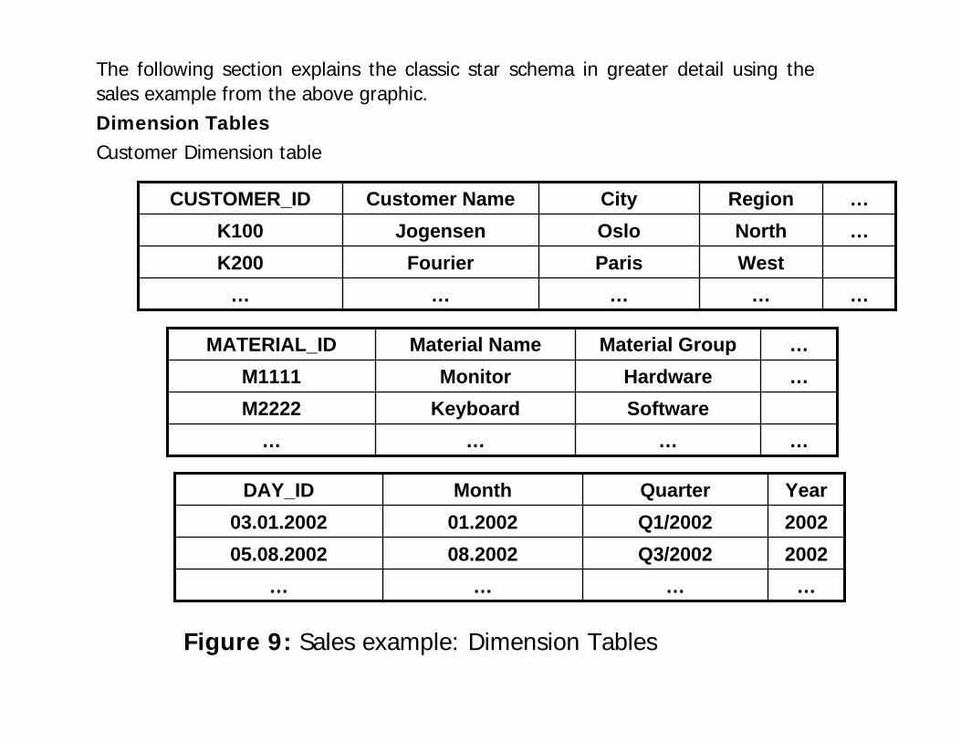
The following section explains the classic star schema in greater detail using the sales example from the above graphic.Dimension Tables Customer Dimension table
……………WestParisFourierK200
…NorthOsloJogensenK100…RegionCityCustomer NameCUSTOMER_ID
…………SoftwareKeyboardM2222
…HardwareMonitorM1111…Material GroupMaterial NameMATERIAL_ID
…………2002Q3/200208.200205.08.20022002Q1/200201.200203.01.2002YearQuarterMonth DAY_ID
Figure 9: Sales example: Dimension Tables
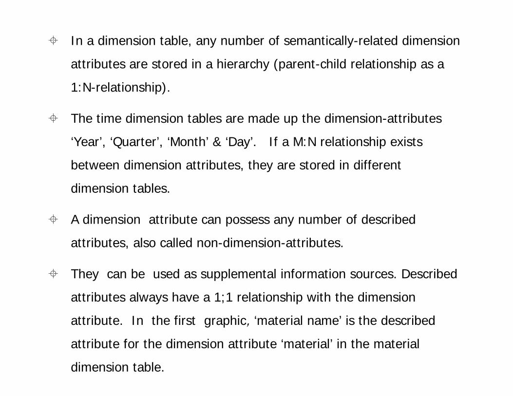
In a dimension table, any number of semantically-related dimension
attributes are stored in a hierarchy (parent-child relationship as a
1:N-relationship).
The time dimension tables are made up the dimension-attributes
‘Year’, ‘Quarter’, ‘Month’ & ‘Day’. If a M:N relationship exists
between dimension attributes, they are stored in different
dimension tables.
A dimension attribute can possess any number of described
attributes, also called non-dimension-attributes.
They can be used as supplemental information sources. Described
attributes always have a 1;1 relationship with the dimension
attribute. In the first graphic, ‘material name’ is the described
attribute for the dimension attribute ‘material’ in the material
dimension table.
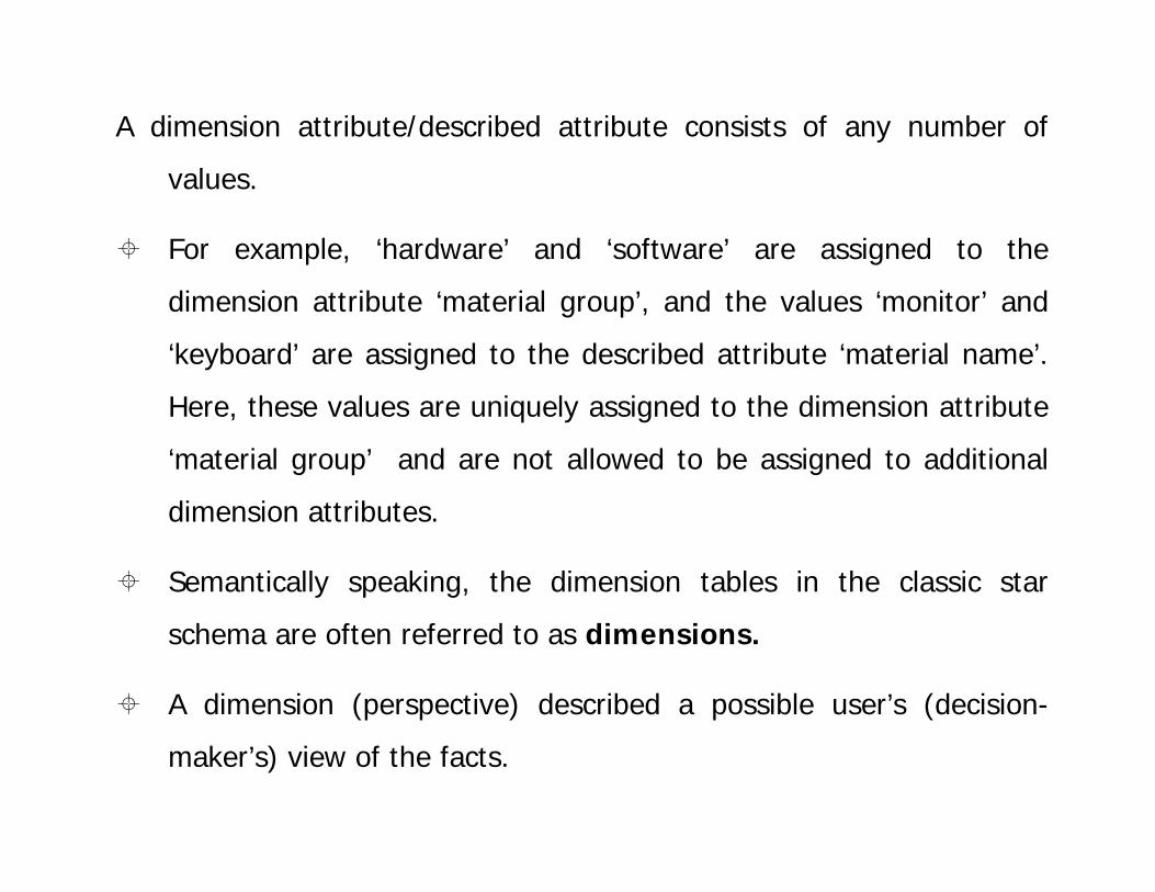
A dimension attribute/described attribute consists of any number of
values.
For example, ‘hardware’ and ‘software’ are assigned to the
dimension attribute ‘material group’, and the values ‘monitor’ and
‘keyboard’ are assigned to the described attribute ‘material name’.
Here, these values are uniquely assigned to the dimension attribute
‘material group’ and are not allowed to be assigned to additional
dimension attributes.
Semantically speaking, the dimension tables in the classic star
schema are often referred to as dimensions.
A dimension (perspective) described a possible user’s (decision-
maker’s) view of the facts.
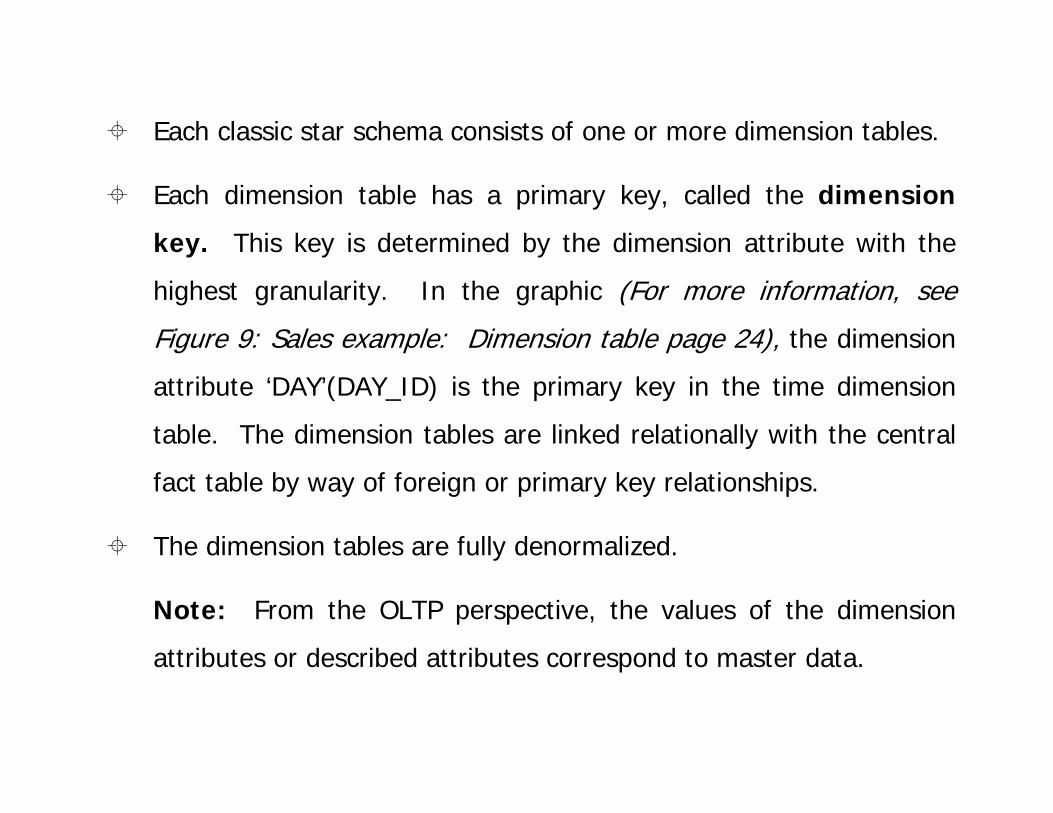
Each classic star schema consists of one or more dimension tables.
Each dimension table has a primary key, called the dimension
key. This key is determined by the dimension attribute with the
highest granularity. In the graphic (For more information, see
Figure 9: Sales example: Dimension table page 24), the dimension
attribute ‘DAY’(DAY_ID) is the primary key in the time dimension
table. The dimension tables are linked relationally with the central
fact table by way of foreign or primary key relationships.
The dimension tables are fully denormalized.
Note: From the OLTP perspective, the values of the dimension
attributes or described attributes correspond to master data.
Fact Table
Fact Table
……………
6300M2222K20005.08.2002
5025.000M1111K10005.08.2002
25010.000M2222K200003.01.2002
250100.000M1111K20003.01.2002
603.000M2222K10003.01.2002
10050.000M1111K10003.01.2002
QuantitySales Volume
MATEIAL_IDCUSTOMER_IDDAY_ID
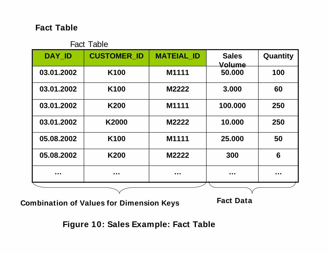
Figure 10: Sales Example: Fact Table
Combination of Values for Dimension Keys Fact Data
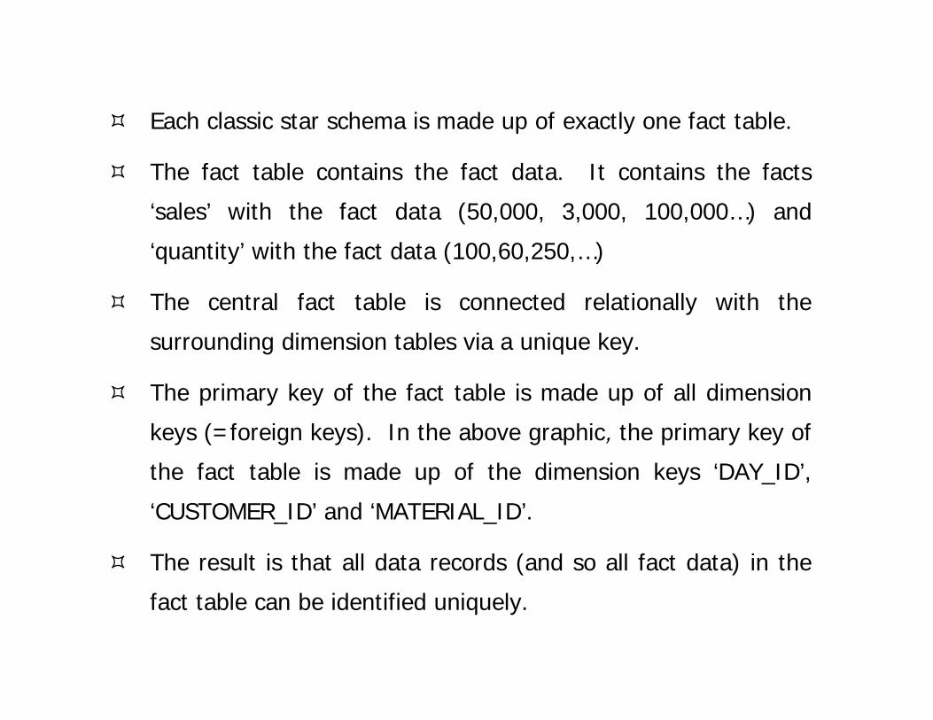
Each classic star schema is made up of exactly one fact table.
The fact table contains the fact data. It contains the facts
‘sales’ with the fact data (50,000, 3,000, 100,000…) and
‘quantity’ with the fact data (100,60,250,…)
The central fact table is connected relationally with the
surrounding dimension tables via a unique key.
The primary key of the fact table is made up of all dimension
keys (=foreign keys). In the above graphic, the primary key of
the fact table is made up of the dimension keys ‘DAY_ID’,
‘CUSTOMER_ID’ and ‘MATERIAL_ID’.
The result is that all data records (and so all fact data) in the
fact table can be identified uniquely.
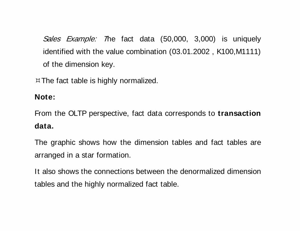
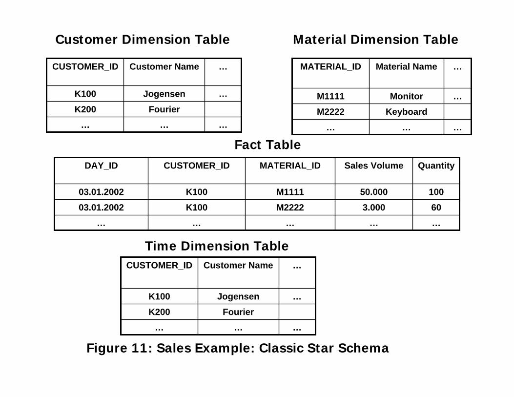
Sales Example: The fact data (50,000, 3,000) is uniquely
identified with the value combination (03.01.2002 , K100,M1111)
of the dimension key.
The fact table is highly normalized.
Note:
From the OLTP perspective, fact data corresponds to transaction
data.
The graphic shows how the dimension tables and fact tables are
arranged in a star formation.
It also shows the connections between the denormalized dimension
tables and the highly normalized fact table.
……………603.000M2222K10003.01.2002
10050.000M1111K10003.01.2002
QuantitySales VolumeMATERIAL_IDCUSTOMER_IDDAY_ID
………FourierK200
…JogensenK100
…Customer NameCUSTOMER_ID
………KeyboardM2222
…MonitorM1111
…Material NameMATERIAL_ID
………FourierK200
…JogensenK100
…Customer NameCUSTOMER_ID
Fact Table
Figure 11: Sales Example: Classic Star Schema
Time Dimension Table
Customer Dimension Table Material Dimension Table
Storing data in the form of the classic star schema is optimized for
reporting. It allows the user to view facts from a variety of perspectives
(Dimensions). A user may be interested in getting answers to the
following questions:
Who have we sold to?
What have we sold?
How much have we sold?
When did we sell it?
From this request, the system generates a three-dimensional results
structure, which can be depicted graphically as a three-dimensional (data)
cube.
The structure of this kind of data cube is determined by the number of
dimensions, the values of the individual dimensions attributes and the
assigned cube cells.
The dimension attribute values represent the coordinates via which
the cells can be accessed uniquely.
The cells only contains one entry for a particular fact. In the above
graphic, the “selected” cell is addressed uniquely via the value
combination (North+South+West+EAST), Hardware, 2002).
This cell contains the fact data 4,000,000(sales) and 3,000(quantity).
Multi-dimensional analysis techniques (OLAP functions) can be used to
define a variety of views on the data cube/multi-dimensional data
structure.
Not all decision-makers have or need the same view of the data.
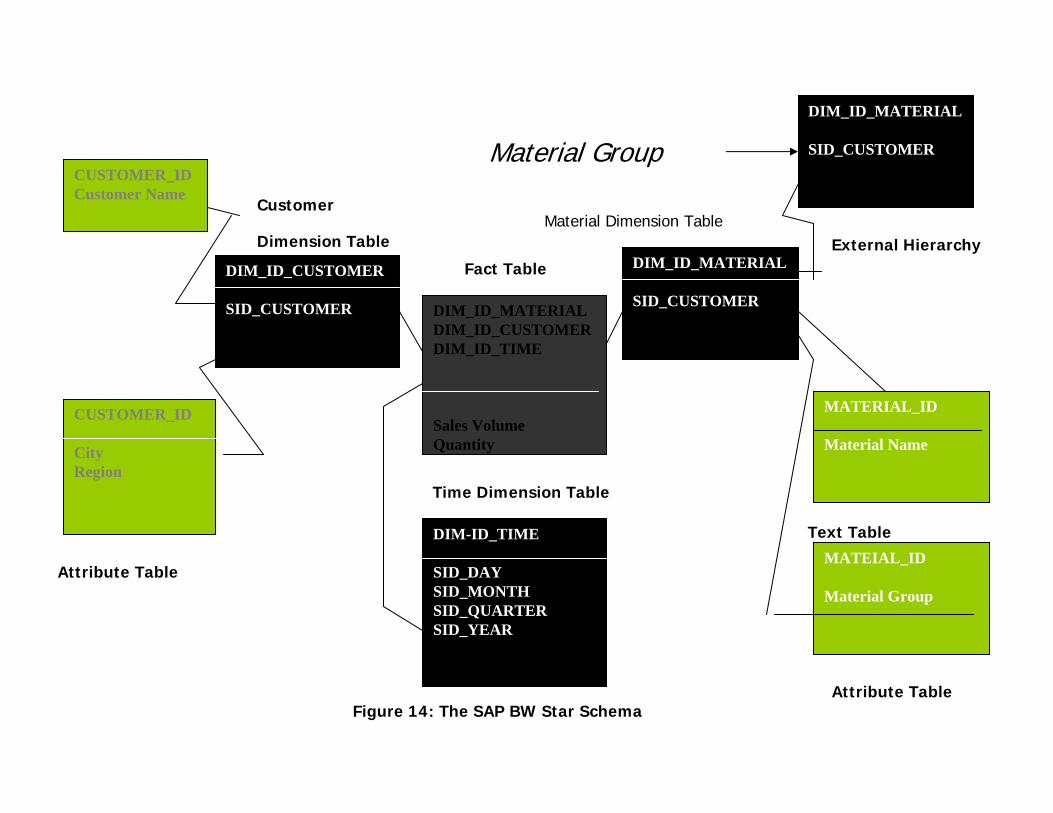
The SAP BW Star Schema• The multi-dimensional model in SAP BW is based on the SAP BW
star schema, which was developed as an enhanced (refined) star schema as a response to problems experienced with the classic star schema.
• The following graphic shows the crossover between the classic star schema and the SAP BW star schema, using the same sales example from the first diagram.
• For the time being, only components relevant to the modeling view are taken into consideration.
DIM_ID_MATERIALDIM_ID_CUSTOMERDIM_ID_TIME
Sales VolumeQuantity
DIM-ID_TIME
SID_DAYSID_MONTHSID_QUARTERSID_YEAR
Time Dimension Table
Figure 14: The SAP BW Star Schema
Fact Table
CUSTOMER_IDCustomer Name
CUSTOMER_ID
CityRegion
DIM_ID_CUSTOMER
SID_CUSTOMER
DIM_ID_MATERIAL
SID_CUSTOMER
Material Dimension Table
DIM_ID_MATERIAL
SID_CUSTOMERMaterial Group
MATERIAL_ID
Material Name
MATEIAL_ID
Material Group
External Hierarchy
Text Table
Attribute Table
Attribute Table
Customer
Dimension Table
• This graphic shows how the SAP BW-star schema is an enhancement of the classic star schema.
• The enhancement comes from the fact that the dimension tables do not contain master data information.
• This master data information is stored in separate tables, called master data tables.
• This section firstly explains the SAP BW-Star Schema in detail.
• At the end of the section, both star schemas are compared in terms of their advantages and disadvantages.
• In the SAP BW-star schema, the distinction is made between two self-contained areas:– InfoCube– Master Data Tables/Surrogate ID (SID-) Tables
InfoCube
InfoCubes are the central objects of the multi-dimensional model in SAP BW. Reports and analyses are based on these. From a reporting perspective, an InfoCube describes a self-contained data set within a business area, for which you can define queries.
An InfoCube (BasicCube) consists of a number of relational tables that are combined on a multi-dimensional basis. In other words, in consists of a central fact table and several surrounding dimension tables.
Hint: There are various types of InfoCube in BW. The InfoCube with type BasicCube is the InfoCube relevant for modelling, since only physical objects (objects that contain data) are considered in the modeling within the SAP BW-data model. For this reason, InfoCube always refers to BasicCube in this section. (You can find additional information about other cube types in the Virtual Cubes lesson).
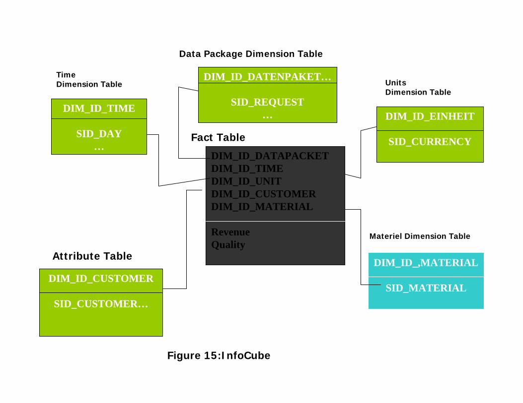
DIM_ID_DATAPACKETDIM_ID_TIMEDIM_ID_UNITDIM_ID_CUSTOMERDIM_ID_MATERIAL
RevenueQuality
Figure 15:InfoCube
Fact Table
DIM_ID_TIME
SID_DAY…
DIM_ID_CUSTOMER
SID_CUSTOMER…
Attribute Table
DIM_ID_DATENPAKET…
SID_REQUEST…
Data Package Dimension Table
DIM_ID_EINHEIT
SID_CURRENCY
DIM_ID_,MATERIAL
SID_MATERIAL
Materiel Dimension Table
Units Dimension Table
TimeDimension Table
SAP BW Star Schema• In the SAP BW-star schema, the facts in the fact table are
referred to as Key figures and the dimension attributes as characteristics.
• The dimension table are linked relationally with the central fact table by way of foreign or primary key relationships.
• In contrast to the classic star schema, characteristics are not components of the dimension tables, in other words, the characteristic values are not stored in the dimension tables.
• A numerical SID key is generated for each characteristic.• This foreign key replaces the characteristic as the
component of the dimension table.• Here, SID stands for Surrogate ID (replacement key).
• In the graphic above, these keys are given the prefix SID_. For example, ‘SID_MATERIAL”, is the SID key for the characteristic ‘MATEIAL’ (‘MATERIAL_ID’).
• Each dimension table has a generated numerical ‘primary key’, called the dimension key.
• In the graphic above, this dimensions key is denoted with the prefix DIM_ID_.
• Here, ‘DIM_ID_MATERIAL’ is the dimension key for the material dimension table. As in the classic star schema, the primary key of the fact table is made up dimension keys (‘DIM_ID_DATENPAKET’,’DIM_ID_ZEIT’,DIM_ID_EINHEIT’,’DIM)ID_KUNDE’,’DIM_ID_MATERIAL’).
• Master Data Tables/SID Tables• Additional information about characteristics is
referred to as master data in the SAP BW. A distinction is made between the following master data types:
• Attributes• Texts• (External) Hierarchies
Master Data Tables/SID Tables• Master data information is stored in separate tables, that is
independent of InfoCube, in what are called Master data tables (separately for attributes, texts and hierarchies).
• In the following graphic, for example, the attribute ‘material group’ is stored in the attribute table, the text description for ‘material name’is stored in the text table and the material hierarchy is stored in the Hierarchy table for the characteristic ‘MATERIAL’.
• In this way, the characteristic ‘MATERIAL’ is the primary key for the master data tables belonging to this characteristic.
• As was already mentioned in the InfoCubes section above, precisely one numerical SID key is assigned to each characteristic.
• This assignment is made in a SID table for the respect characteristic, whereby the characteristic becomes the primary key in the SID table.
• In the following graphic, the SID key ‘SID_MATERIAL’ is assigned to the characteristic ‘MATERIAL’ in the SID table for characteristic ‘MATERIAL’.
• The SID table is connected to the associated master data tables via the characteristic key.
• Hint: By using the term ‘Hierarchy’, we usually mean an arrangement of objects having a 1:N relationship to each other.
• In this sense, there are hierarchies in the dimension-, attribute-and hierarchy tables in BW.
• This ‘hierarchy’ term is strongly connected with the ‘drilldown’ term (pre-defined drilldown path) in data warehousing terminology.
• However, in the SAP BW, the term “drilldown’ can also be used without referring to a hierarchy.
• In SAP BW, under “external hierarchies”, we mean presentation hierarchies, which are stored in what are called hierarchy tables as a structure for characteristic values.
Connecting Master Data Tables to an InfoCube
• Master data tables are connected to an InfoCube (and thus to the key figures of the fact table) by way of the SID tables.
• The excavation of master data from the dimension tables using SID technology allows you to use the master data with different InfoCubes.
• In other words, the master data is InfoCube-independent, and can be used by several InfoCubes at the same time.
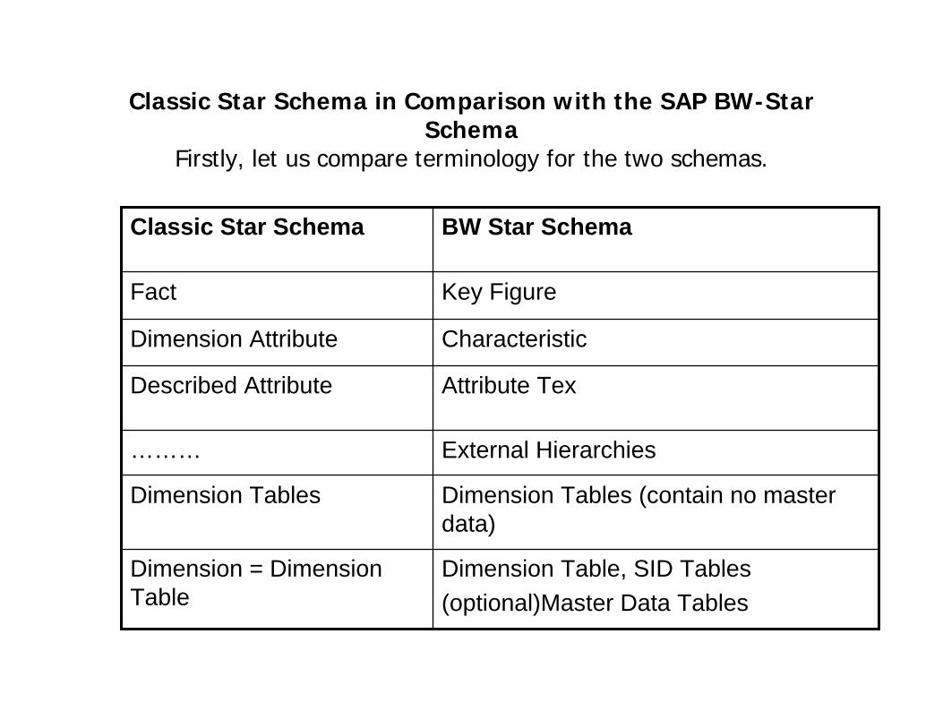
Classic Star Schema in Comparison with the SAP BW-Star Schema
Firstly, let us compare terminology for the two schemas.
Dimension Table, SID Tables(optional)Master Data Tables
Dimension = Dimension Table
Dimension Tables (contain no master data)
Dimension Tables
External Hierarchies………
Attribute TexDescribed Attribute
CharacteristicDimension Attribute
Key FigureFact
BW Star SchemaClassic Star Schema
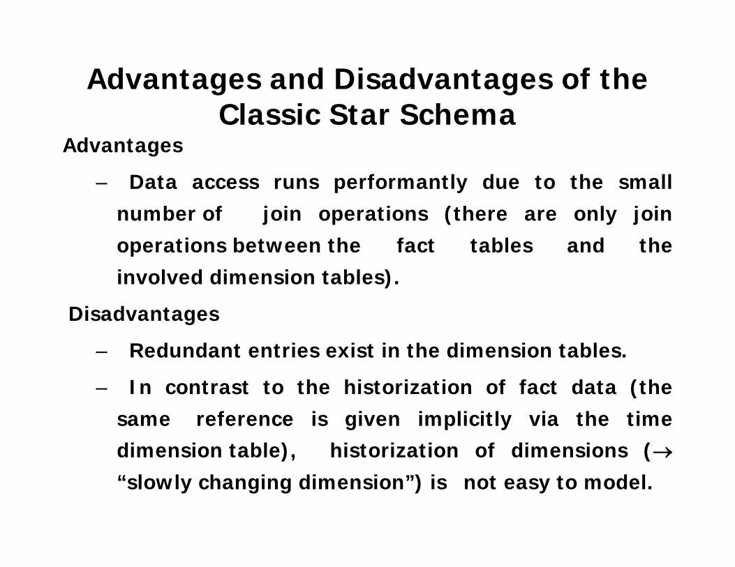
Advantages and Disadvantages of the Classic Star Schema
Advantages
– Data access runs performantly due to the small number of join operations (there are only join operations between the fact tables and the involved dimension tables).
Disadvantages
– Redundant entries exist in the dimension tables.
– In contrast to the historization of fact data (the same reference is given implicitly via the time dimension table), historization of dimensions (→“slowly changing dimension”) is not easy to model.
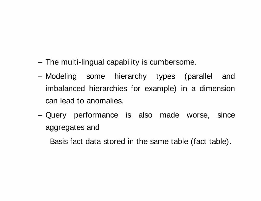
– The multi-lingual capability is cumbersome.
– Modeling some hierarchy types (parallel and
imbalanced hierarchies for example) in a dimension
can lead to anomalies.
– Query performance is also made worse, since
aggregates and
Basis fact data stored in the same table (fact table).
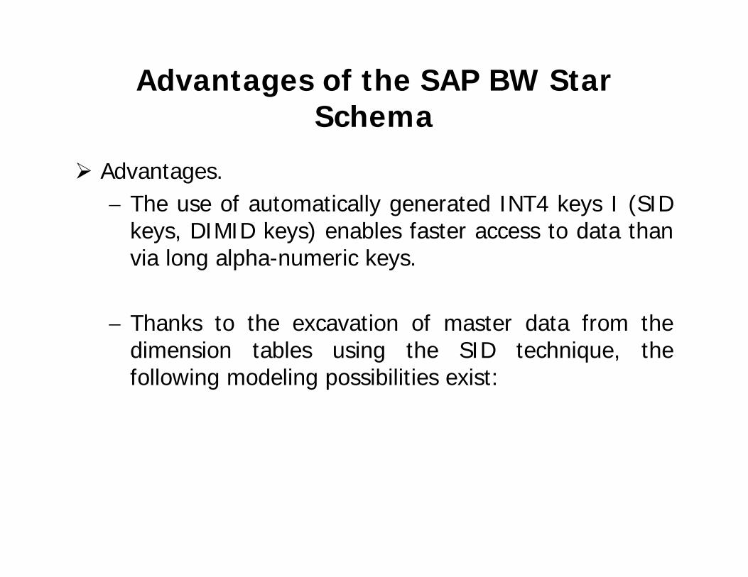
Advantages of the SAP BW Star Schema
Advantages.− The use of automatically generated INT4 keys I (SID
keys, DIMID keys) enables faster access to data than via long alpha-numeric keys.
− Thanks to the excavation of master data from the dimension tables using the SID technique, the following modeling possibilities exist:
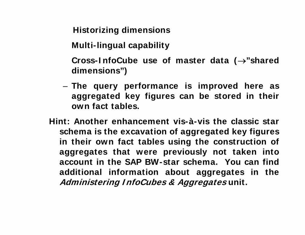
Historizing dimensions
Multi-lingual capability
Cross-InfoCube use of master data (→”shared dimensions”)
– The query performance is improved here as aggregated key figures can be stored in their own fact tables.
Hint: Another enhancement vis-à-vis the classic star schema is the excavation of aggregated key figures in their own fact tables using the construction of aggregates that were previously not taken into account in the SAP BW-star schema. You can find additional information about aggregates in the Administering InfoCubes & Aggregates unit.
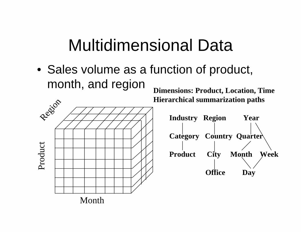
Multidimensional Data• Sales volume as a function of product,
month, and region
Prod
uct
Region
Month
Dimensions: Product, Location, TimeHierarchical summarization paths
Industry Region Year
Category Country Quarter
Product City Month Week
Office Day
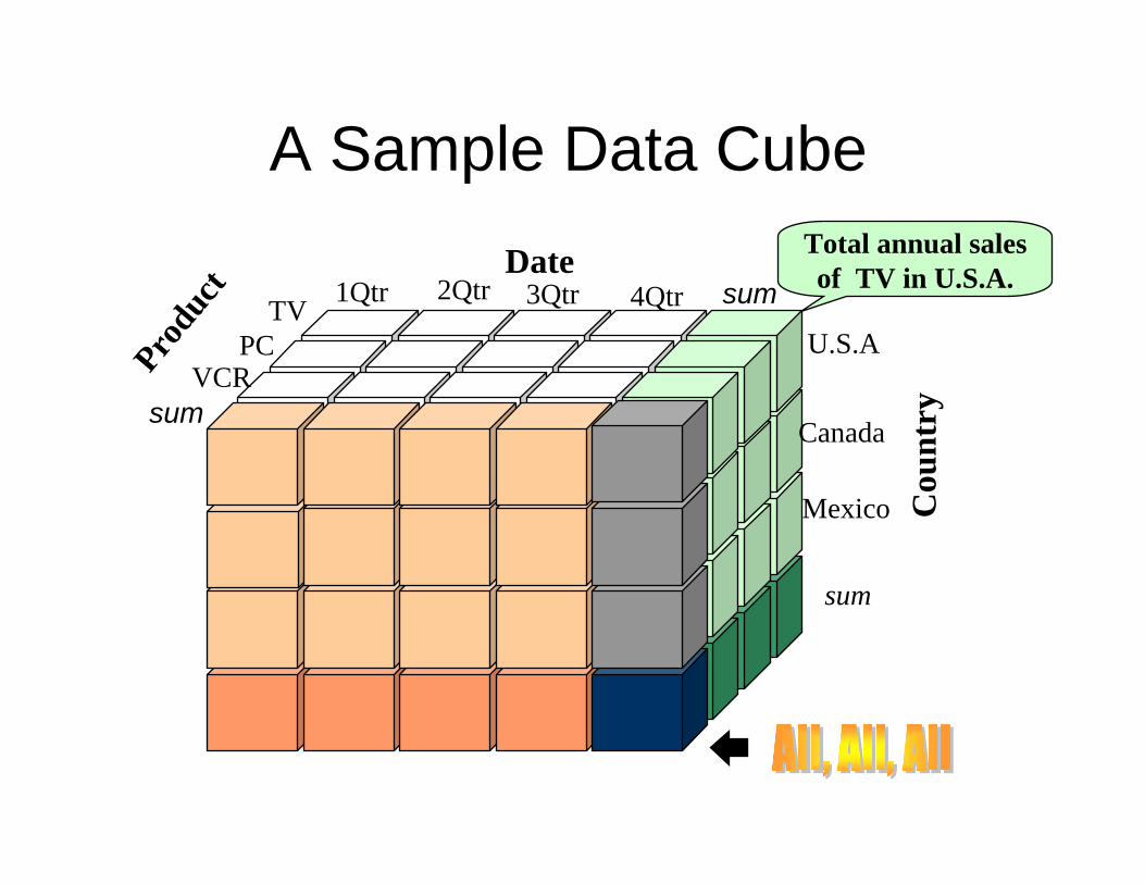
A Sample Data CubeTotal annual salesof TV in U.S.A.Date
Produ
ct
Cou
ntrysum
sumTV
VCRPC
1Qtr 2Qtr 3Qtr 4QtrU.S.A
Canada
Mexico
sum
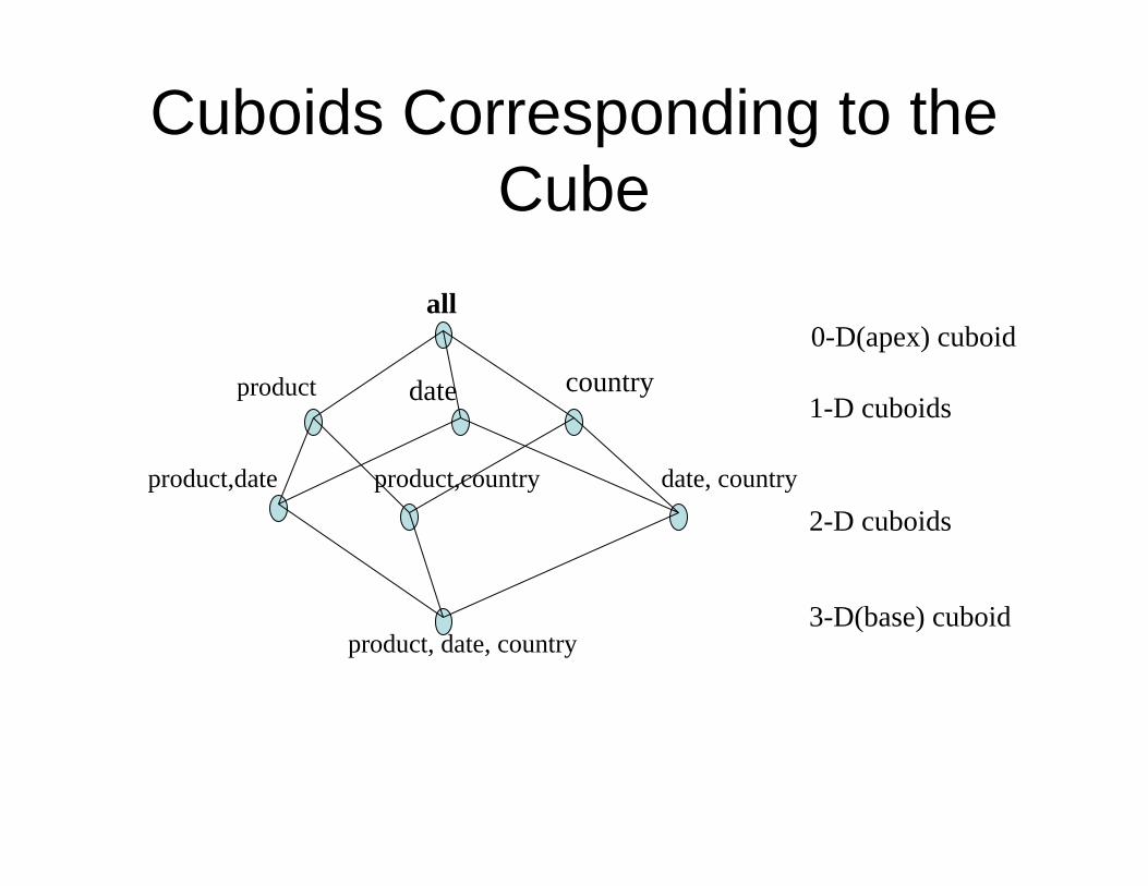
Cuboids Corresponding to the Cube
all
product date country
product,date product,country date, country
product, date, country
0-D(apex) cuboid
1-D cuboids
2-D cuboids
3-D(base) cuboid
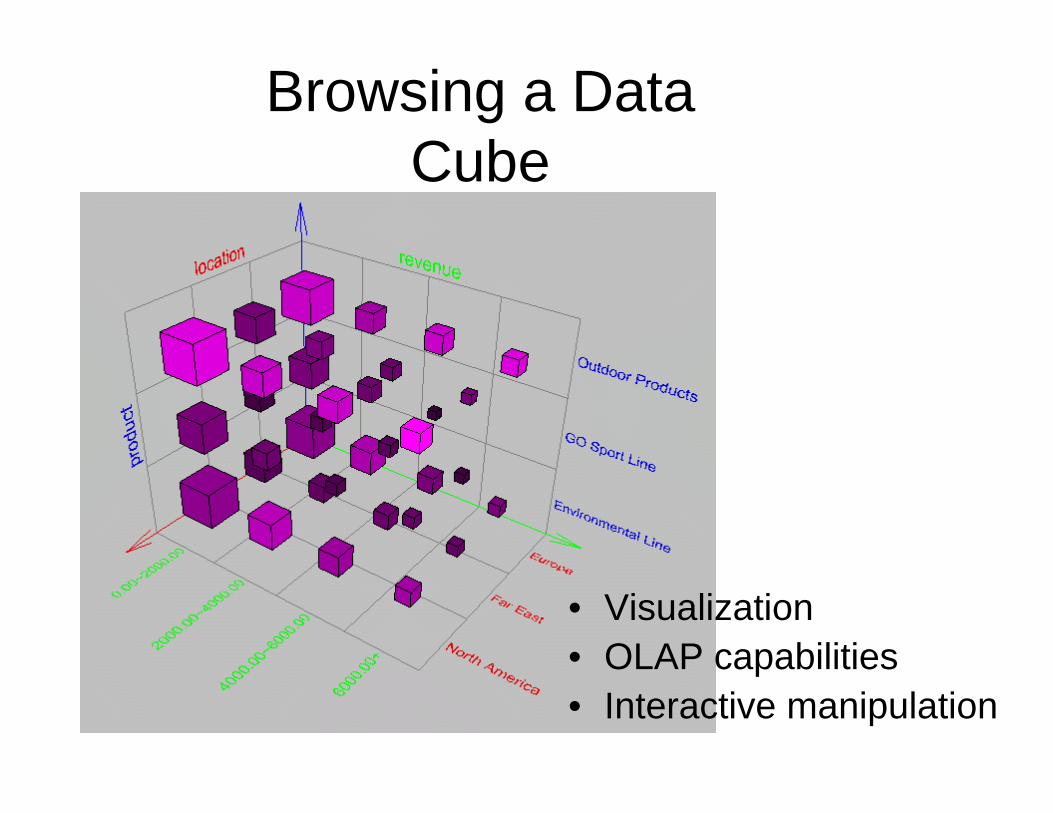
Browsing a Data Cube
• Visualization• OLAP capabilities• Interactive manipulation
Metadata Repository• Meta data is the data defining warehouse objects. It has
the following kinds – Description of the structure of the warehouse
• schema, view, dimensions, hierarchies, derived data definition, data mart locations and contents
– Operational meta-data• data lineage (history of migrated data and transformation path),
currency of data (active, archived, or purged), monitoring information (warehouse usage statistics, error reports, audit trails)
– The algorithms used for summarization– The mapping from operational environment to the data warehouse– Data related to system performance
• warehouse schema, view and derived data definitions– Business data
• business terms and definitions, ownership of data, charging policies
• Data warehouse– A subject-oriented, integrated, time-variant, and nonvolatile collection of
data in support of management’s decision-making process
• A multi-dimensional model of a data warehouse– Star schema, snowflake schema, fact constellations– A data cube consists of dimensions & measures
• OLAP operations: drilling, rolling, slicing, dicing and pivoting
• OLAP servers: ROLAP, MOLAP, HOLAP• Efficient computation of data cubes
– Partial vs. full vs. no materialization– Multiway array aggregation– Bitmap index and join index implementations
• Further development of data cube technology– Discovery-drive and multi-feature cubes– From OLAP to OLAM (on-line analytical mining)
End of Multi Dimensional Model
SAP BIW
Administrator Workbench (AWB) I
Lesson Objectives
After completing this lesson, you will be able to:
explain how the AWB Initial Screen is structured
describe the tasks of the AWB
give an overview of the functional areas in the AWB.
Business Example
In your BW project team, you have been given the task of defining meta
objects in the SAP BW system. You would like to get an overview of
the AWB tool.
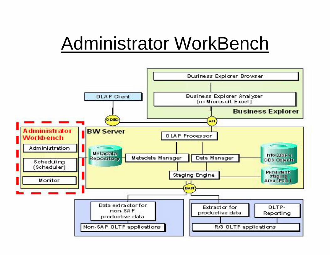
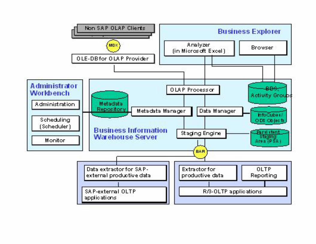
Administrator WorkBench
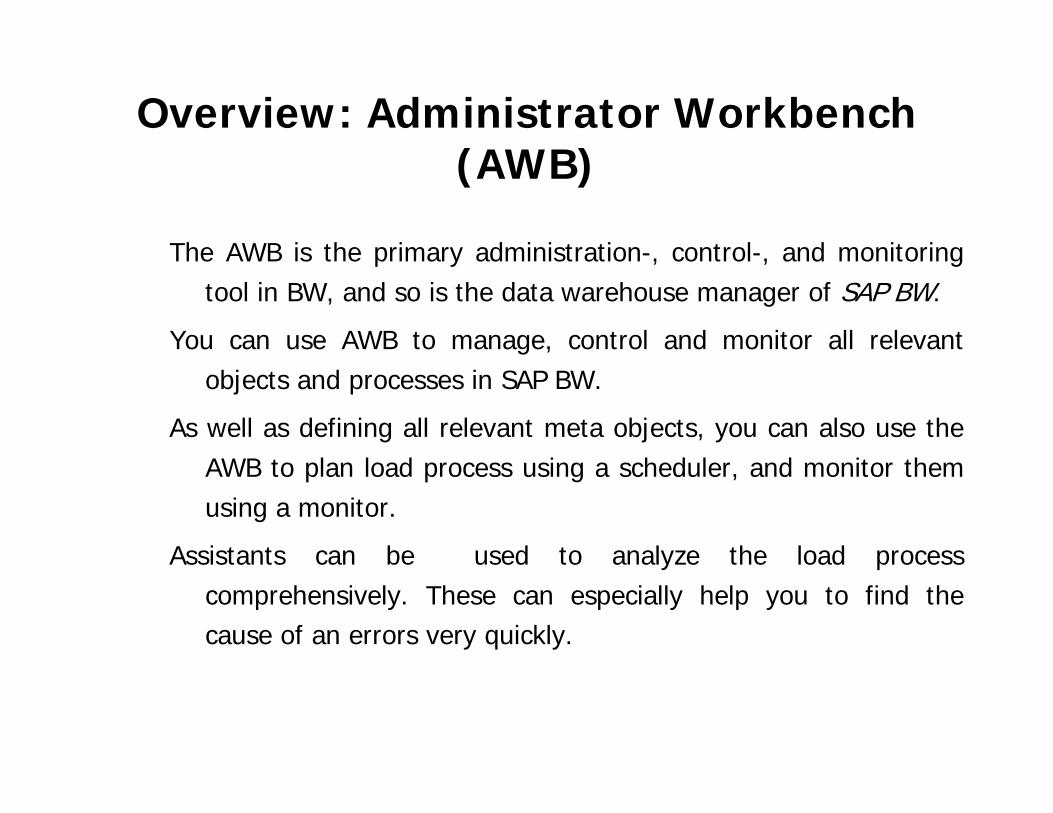
Overview: Administrator Workbench (AWB)
The AWB is the primary administration-, control-, and monitoring tool in BW, and so is the data warehouse manager of SAP BW.
You can use AWB to manage, control and monitor all relevant objects and processes in SAP BW.
As well as defining all relevant meta objects, you can also use the AWB to plan load process using a scheduler, and monitor them using a monitor.
Assistants can be used to analyze the load process comprehensively. These can especially help you to find the cause of an errors very quickly.
Functional Areas
You perform tasks in AWB in the following function areas :
Modeling
Monitoring
Reporting Agent
Transport Connection
Documents
Business Content
Translation
Metadata Repository
ModelingModeling
The Modeling functions area is used to create and maintain (meta) objects relevant to the data staging process in SAP BW. These objects are displayed in a tree structure, in which the objects are ordered according to hierarchical criteria. You can use a context menu to access the relevant maintenance dialogs for each object in the object tree. You can also carry out additional functions.
To access the Modeling functions area, choose transaction RSA1.
Monitoring
The Monitoring function area enables you to
monitor and control data loading processes and
additional data processes in SAP BW.
You can access the Monitoring function area via the
transaction RSMON.
Reporting Agent
The Reporting Agent is a tool with which you can schedule and
execute reporting functions in the background, such as the
evaluation of exceptions, the printing of queries and the
pre-calculation of Web templates.
To access the Reporting Agent function area, in the AWB
navigation box, choose Reporting Agent.
Documents
Documents
The Documents function are enables you to insert, search in, and create links
for one or more documents in various formats, versions and languages for
SAP BW objects. You can find detailed information about SAP BW-
document distribution in the BW305 (BW Reporting Analysis) or TBW20
courses, and in the online documentation.
To access the Documents function area, in the AWB navigation window, choose
Documents.
Business Content
Business Content
Business Content provides pre-configured information models based on
metadata. It provides users in an enterprises with a selection of
information they can use to fulfill their tasks. (You can find
additional information about Business Content in the Business
Content Unit.)
To access the Business Content function area, choose the transaction
RSORBCT.
Translation
In the Translation function area, you can translate short and long texts
belonging to SAP BW-objects to any language that are supported in
SAP BW.
To access the Translation function area, in the AWB navigation
window, choose Translation.
Metadata Repository
In the HTML-based SAP BW-Metadata Repository, all SAP BW meta objects
and the corresponding links to each other are managed centrally.
Together with an integrated Metadata Repository browser, a search
function is available enabling a quick access to the meta
objects. In addition, metadata can also be exchanged between
different systems, HTML pages can be exported, and graphics
for the objects in the displayed.
To access the Metadata Repository function area, choose the
transaction RSOR.
InfoObjects
Lesson Objectives
After completing this lesson, you will be able to:
explain the important of InfoObjects in SAP BW.
classify InfoObjects.
define InfoObjects.
The Importance of InfoObjects in SAP BW
InfoObjects are the “smallest available information modules” (=fields) In
SAP BW: These can be uniquely identified with their technical name.
As components of the Metadata Repository, InfoObjects contain the
technical and specialist information for master-and transaction data in
SAP BW.
InfoObjects are used throughout the system to create structures and
tables. These enables information to be modeled in a structured form
in SAP BW.
InfoObjects are used for the definition of reports, to evaluate
master-and transaction data.
Hint: SAP delivers InfoObjects within Business Content (BCT).
The technical name of standard InfoObjects begins with 0. As
well as these, you can also define your own InfoObjects. Make
sure the technical name begins with a letter between A and Z
and that it is 3-9 characters in length.
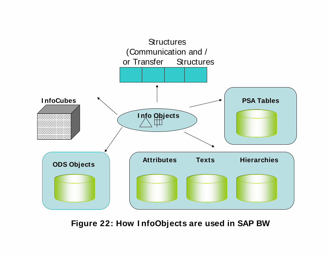
Structures(Communication and /
or Transfer Structures
ODS ObjectsAttributes Texts Hierarchies
PSA Tables
Figure 22: How InfoObjects are used in SAP BW
Info Objects
InfoCubes
Characteristics
Characteristic InfoObjects are business reference objects, which
are used to analyze key figures.
Classifying InfoObjects
InfoObjects are divided into the following classes:
Key Figures
Key figure InfoObjects provide the values to be evaluated.
Example:
– Quantity (0QUANTITY)
– Amount (0AMOUNT)
Time Characteristics
Time characteristics form the time reference frame for many data analysis
and evaluations. They are delivered with Business Content. It is not
possible to define your own time characteristics.
Examples:
- Time characteristic with the largest granularity: Calendar Day
(0CALDAY)
Time characteristic with the smallest granularity: Calendar Year (0CALYear)
Hint: Once again, it is not possible to define your own time characteristics.
Units
Unit InfoObjects can be specified alongside the key figures. They
enable key figure values to be partnered with their corresponding
units in evaluations.
Examples:
- Currency unit (0CURRENCY)
- Value Unit (0UNIT)
Technical Characteristics
These characteristics have an organizational function
within SAP BW.
Examples:
- Request ID (0REQUID)
- Change ID (0CHNGID)
Info Object 0REQUID delivers the numbers the system
allocates when loading requests ; Info Object 0CHNGID
delivers the numbers allocated during aggregate change
runs.
Info Object Tabs
General
Business Explorer
Master data /texts
Attributes
Hierarchy
Compounding
General
General
This tab page is used to determine the basic properties of a
characteristic for example description, data type (CHAR, NUMC,…),
length (max, 60 characters) and conversion routine.
Hint: When defining a characteristic, you must enter at lest a
description data type and length. All other settings on this and
other tab pages are optional.
Business Explorer (BEx)
Business Explorer (BEx)
This tab page is used to set the display defaults in the
Business Explorer (BEx).
That is, to determine whether or not the characteristic is
to appear as a textual description or as a key in BEx by
default.
Master Data/texts
Master Data/texts
On this tab page, you determine whether or not the characteristic can
have attributes or texts.
If the characteristic is to have its own texts, you need to make at least
one text selection (short, medium-length, long text-20,40,60
characters).
The attributes are assigned to the characteristic on the Attributes tab
page.
Attributes
Attributes
Attributes are themselves InfoObjects (characteristics/key figures) that
are used to describe characteristics in greater detail.
For example, the characteristic cost center can be described in more
detail with profit center and controlling area to which it is assigned.
Here the attributes are themselves InfoObjects (characteristics/key
figures).
If the With master data indicator was set on the Master data/texts tab
page, you are able to specify attributes and properties for these
attributes together with the characteristic on the Attributes tab page.
Display Attributes
Display Attributes:
If you define attributes as display attributes, you can only use these
attributes as additional information in reporting when combined with
the characteristic.
In other words, in reporting, you cannot navigate with in the dataset of
a data target (InfoCube / ODS object).
Navigation Attributes
Navigation Attributes
If you define attributes as navigation attributes, you are able to use these
to navigate in reporting. When a query is executed, the system does
not distinguish between navigation attributes and characteristics for a
data target (InfoCube/ODS Object).
In other words, all navigation functions in the query are also possible for
navigation attributes. In order to make these attributes available as
navigation attributes in reporting, you need to activate them once more
on a data target (InfoCube/ODS object) level. Otherwise, the
attributes function as display attributes.
Time Dependency
Time Dependency
Switch attributes (display/navigation attributes) to ‘time-dependent’ if a
validity area is required for each attribute value.
Hint:
If a characteristic Info Object is defined as Attribute Only. You can
only use this characteristic Info Object as a display attribute for
another characteristic.
The extensive use of navigation attributes leads to large number of
tables and joins, which can reduce performance. (You can find
additional information in the Technical Implementation in SAP BW
lesson.
A characteristic that is used as a navigation attribute can also have
its own navigation attributes.
These are called transitive attributes (navigation attributes with
two levels).
You can activate these as well, thus making them available for
reporting.
ExampleHierarchies are used to analysis of describe alternative views of the
data. A hierarchy comprises a quantity of nodes and leaves. The
nodes stand in a parent-child relationship and the hierarchy leaves are
represented by the characteristic values. On the Hierarchy tab page,
you determine whether or not the characteristic can have hierarchies,
and if so, what properties These hierarchies are allowed to have.
If the With hierarchies indicator is set, hierarchies can be
created for this characteristic within SAP BW (choose
transaction BSH1). Alternatively, they can be loaded from SAP
R/3 or flat files.
Hint:
To repeat what was said earlier, in SAP BW, by “external
hierarchies”, we means presentation hierarchies that are stored in
what are called hierarchy tables as a structure for characteristic
values.
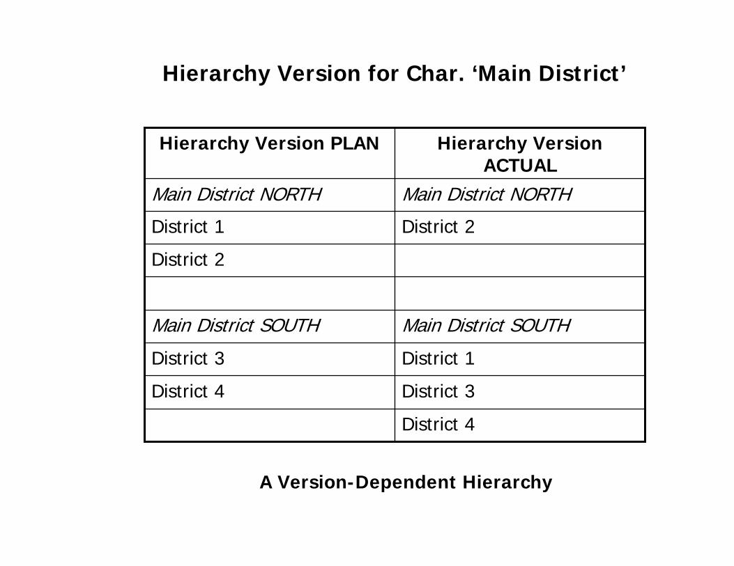
A Version-Dependent Hierarchy
A Version-Dependent Hierarchy
Characteristic hierarchies can be used in different hierarchy
versions. Different hierarchy versions that exist in the source
system can be modeled in SAP BW. However, you can
also create different versions for one and the same hierarchy
from the source system. These versions can then compared
with one another in a query.
Example:
During restructuring of an organization’s sales districts for the
“main district” characteristic, several hierarchy versions are
created. These can be compared to each another in a query.
Hierarchy Version for Char. ‘Main District’
District 4
District 3District 4
District 1District 3
Main District SOUTHMain District SOUTH
District 2
District 2District 1
Main District NORTHMain District NORTH
Hierarchy Version ACTUAL
Hierarchy Version PLAN
A Version-Dependent Hierarchy
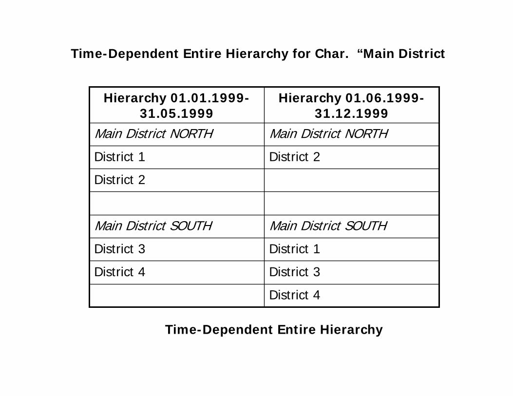
A Time-Dependent Entire Hierarchy
A Time-Dependent Entire Hierarchy
You determine here whether the entire hierarchy is allowed to be
time-dependent. In other words, there are versions for this
hierarchy that are valid for a specific time interval. The system
automatically chooses the valid version.
Example:
During restructuring of an organization’s sales districts for the “main
district” characteristic, the hierarchy is made time-dependent. This
enables this restructuring to be compared for different times in a
query.
District 4
District 3District 4
District 1District 3
Main District SOUTHMain District SOUTH
District 2
District 2District 1
Main District NORTHMain District NORTH
Hierarchy 01.06.1999-31.12.1999
Hierarchy 01.01.1999-31.05.1999
Time-Dependent Entire Hierarchy for Char. “Main District
Time-Dependent Entire Hierarchy
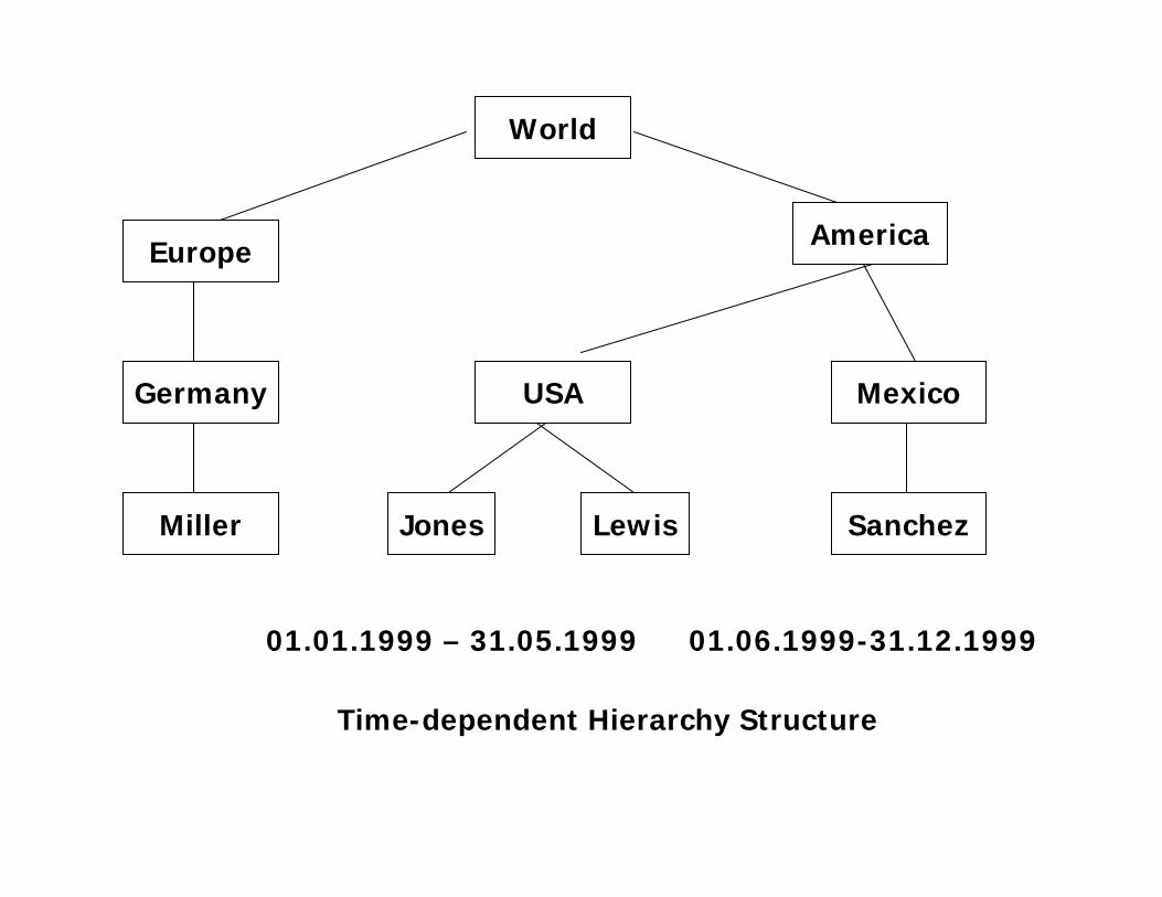
Time-Dependent Hierarchy Structure
Time-Dependent Hierarchy Structure
You determine here whether or not the hierarchy structure is
hierarchy node) is to be time-dependent. The hierarchy is then
constructed for the current key date or for the key date
specified in the query.
Example:
During restructuring of an organization’s sales districts, it was
found that an employee is assigned to different cost centers at
different times.
World
Europe America
Germany Mexico
Miller Sanchez
USA
Jones Lewis
01.01.1999 – 31.05.1999 01.06.1999-31.12.1999
Time-dependent Hierarchy Structure

Administrator WorkBench
Purpose
• The Administrator Workbench is the tool for controlling, monitoring and maintaining all of the processes connected with data staging and processing in the Business Information Warehouse.
• The Administrator Workbench encompasses the following functional areas:– Modeling– Monitoring– Reporting Agent– Transport Connection– Business Content– Where-Used List– Translation– Metadata Repository