Business Cycle Accounting of the U.S. Economy:

the Pre-WWI Period

Dou Jiang

School of Economics

University of Adelaide

Supervisor: Mark Weder

School of Economics

University of Adelaide

Abstract

What caused the Depression of the 1890s and what caused the 1907 recession

in U.S.? In particular, we apply the Business Cycle Accounting method to

decompose the economic �uctuation into its sources: productivity, the labour

wedge, the investment wedge and the government consumption wedge. Our

results suggest that the economy downturn is primarily attributed to frictions

that reduce productivity and the wedge capturing distortions in labour-leisure

decision. The �nancial market frictions would have accounted for the drop of

the e�ciency wedge. A contractionary monetary shock could generate a gap

between the marginal rate of substitution and the marginal product of labour.

Keywords: Growth model, Business cycle accounting, Pre-WWI

1

Figure 1: Real GNP per Capita in 1889-1913

1890 1892 1894 1896 1898 1900 1902 1904 1906 1908 1910 1912350

400

450

500

550

600

650

700

1 Introduction

The cyclical slumps from 1890 to World War I, overshadowed by the Great Depres-

sion, have been almost forgotten by recent economists. In fact, the 1890s were a

tumultuous period for the United States' macroeconomy. The National Bureau of

Economic Research dates four recessions for the decade: 1890:III-1891:II, 1893:I-

1894:II, 1895:IV-1897:II and 1899:III-1900:IV. The contraction beginning in early

1893 was the hardest and the economy's full recovery was painfully long. To put this

into perspective, per capita output dipped close to 15 percent and the cumulative

economic costs were enormous: it was only by 1901 that the U.S. economy again

reached aggregate output trend observed in 1892. Moreover, the recession in 1907

was the last and one of the deepest recessions during the National Banking Era, which

eventually led to the establishment of the Federal Reserve System. Figure 1 shows

the undetrended real gross national product (GNP) per capita in 1889-1913.1

1Our data is based on an annual basis. To organize our presentation, we focus on the period of1892-1894 as the most severe economic downturns during the 1890s occur in these years. We alsoemphasize the big economic slumps from 1906 to 1908. These years are indicated by shaded areas.

2

What caused the depression of the 1890s and what caused the 1893 and 1907 reces-

sions in U.S.? It is imperative to explore the economic �uctuations during the pre-Fed

period since it is simpler in important respects. Once the Central Bank or govern-

ment intervened in the economy, the analysis would become much more complicated.

Therefore we can concentrate our analysis on the sources of shocks that instigate a

downturn instead of policy responses that may have deepened the contractions.

This paper addresses these questions in the context of a neoclassical model of the

business cycle. In particular, we apply the Business Cycle Accounting (BCA) method

introduced by Chari, Kehoe and McGrattan (2007) to decompose the economic �uc-

tuation into its sources from 1889-1913.

Using this technique we �rst measure the deviations of the real world economic be-

haviour from its best outcome implied by the standard growth model. There are

four types of deviations: the e�ciency wedge is measured as time-varying productiv-

ity or exogenous technology shocks. The labour wedge drives a `wedge' between the

marginal product of labour and the marginal rate of substitution between consump-

tion and leisure. The investment wedge distorts the Euler equation. These wedges at

face value look like `taxes' on labour and investment income. The government con-

sumption wedge is de�ned as the sum of government spending and net export. In a

second step, we pin down the wedges that primarily drive the economic �uctuations.

With the diagnostic information acquired from the �rst stage, we are able to evaluate

the relative importance of these wedges to economic �uctuations by simulating the

models including just one wedge or the combination of wedges. Chari, Kehoe and

McGrattan (2007) illustrate that many models with frictions could be reconstructed

as a neoclassical model incorporating one or more wedges. Therefore the BCA ap-

proach provides useful insight to researchers: it helps them to narrow down the class

3

of models to consider. Lastly, we look for frictions that might a�ect the economy

through these transmission mechanisms (wedges).

We divide our analysis into two sub-periods: 1889-1901 and 1901-1913. Our account-

ing results show that the e�ciency wedge and the labour wedge account for most of

the variations in output, labour hours and investment in U.S. during both sub-periods.

In particular, the e�ciency wedge alone accounts for most of the output behaviour

especially its decline in the 1893 and 1907 recessions. The labour wedge is of second

importance. The labour hours condition, is primarily driven by the labour wedge

which almost �perfectly� predicts the decline of hours in 1894 and 1908, followed by

the e�ciency wedge.

We elabourate on each of these two wedges. First, capital utilization is thought to be

an important determinant of movement in the measured e�ciency wedge, therefore

a promising theory that maps into the e�ciency wedge in the growth model should

take variable capital utilization into account. Besides variable capital utilization,

frictions that captured by the e�ciency wedge are explored. The e�ciency wedge

deteriorates in early 1893, followed by a sluggish recovery, which coincides the number

of business failures. These happened again from 1907 during the second sub-period.

We conclude that �nancial market frictions may be partly responsible for the wedge.

Second, we decompose the labour wedge into the price markup and the wage markup

and illustrate that the wage markup is the dominant aspect of the labour wedge.

We �nd that monetary shocks could be an underlying factor that contributes to the

labour wedge, by inducing substantial wage markup during both recession periods.

The rest of the paper is organized as follows. In Section 2, we describe the framework

of the BCA method including the prototype model and the accounting procedure.

Section 3 presents the accounting results. In Section 4 we discuss the factors that

4

may explain the movements of the wedges and provide some background on our

sample periods. Section 5 concludes.

2 Business Cycle Accounting

2.1 The Prototype Growth Model

In this section we describe a neoclassical growth model used in Business Cycle Ac-

counting. This model incorporates four stochastic wedges: the e�ciency wedge, the

labour wedge, the investment wedge, and the government consumption wedge. These

are measures capturing the overall distortion to the optimal decisions made by agents

in perfectly competitive markets.

2.1.1 Household and Firm

The economy consists of identical in�nitely-lived households who are endowed with

one unit of time in each period. They choose per capita consumption ct, supply of

labour service ht and per capita physical capital kt, taking rent rt and real wage rate wt

as given. Firms produce goods choosing capital and labour to maximize their pro�ts.

Households own the �rms and therefore the pro�ts are remitted to households. Time

evolves discretely. The population grows at a constant rate gn; the deterministic rate

of technological progress is given by gz.

A representative household maximizes the present discounted value of his lifetime

utility

maxct,ht,kt+1

Et

∞∑t=0

βt(1 + gn)tu(ct, 1− ht),

5

subject to the budget constraint

ct + (1 + τxt)xt = (1− τht)wtht + rtkt,

where xt is per capita investment in new capital, β is the discount factor parameter.

τxt and τht denote the imaginary investment tax rate and labour tax rate, respectively.

At face value the labour wedge and investment wedge behave like taxes levied from

agent's labour and investment income. The measure of the labour wedge and invest-

ment wedge are given by 1− τlt and 1/(1 + τxt). These wedges are taxes that distort

the agent's �rst order conditions and prevent the economy from its best outcome. In

the absence of market frictions, the value of these wedges should be equal to one.

Given the depreciate rate δ, the law of motion for capital accumulation is given by

(1 + gz)(1 + gn)kt+1 = (1− δ)kt + xt.

The representative �rm's problem is to maximize its pro�t subject to its technology:

maxkt,ht

yt − rtkt − wtht.

2.1.2 Equilibrium

In this model, the household's preference is represented by

u(ct, 1− ht) = logct + θlog(1− ht),

6

where θ is a time allocation parameter. Firm produces single output with a Cobb-

Douglas production function

y = kαt (ztht)1−α,

where α stands for the capital share parameter and zt denotes the productivity shock.

z1−α captures the e�ciency wedge.

The equilibrium in this economy is de�ned as a set of prices {rt, wt}∞t=0 and a set

of allocations {ct, ht, kt, xtyt}∞t=0 satisfying household and �rm's �rst order conditions

and their budget constraints. Therefore the economy can be summarized as the

following equilibrium equations:

θct1− ht

=(1− τht)(1− α)yt

ht, (1)

1

ct(1 + τxt)(1 + gz) = Et{

β

ct+1

[αyt+1

kt+1

+ (1 + τxt+1)(1− δ)]}, (2)

y = kαt (ztht)1−α, (3)

yt = ct + xt + gt. (4)

Equation (1) shows the intratemporal labour-consumption trade o�. Equation (2) is

the consumption Euler equation. Equation (3) and (4) are the production function

and the resource constraint faced by the economy. gt refers to per capita government

spending plus net export and is measured as the government consumption wedge.

2.2 Accounting Procedure

In this subsection, we apply the accounting procedure to the U.S. economy during

1889-1913 which contains two major business cycle episodes: the depression of the

7

1890s and the 1907 recession periods. Therefore we divide it into two sub-periods:

1889-1901 and 1901-1913. We �rstly derive the series of these four wedges and then

feed them back into the prototype growth model to assess the marginal contribution

of one wedge or the combination of wedges to the observed �uctuations of output,

labour and investment.

The wedges are measured from the data. The primary data source we use is Kendrick

(1956) which gives us the annually time series of output, labour, consumption and

investment. The data of investment consists of gross private domestic investment,

consumption durables and net factor payments. Capital data is constructed using

perpetual inventory method. This method requires an initial value of capital. We

set k1892 as initial capital which is chosen such that the capital-output ratio in year

1892 matches the average capital-output ratios during 1892-1929. Then we generate

a time series of capital stock using the capital accumulation law.

In the prototype model all variables are de�ned in terms of detrended per capita. Thus

these variables are divided by resident population to obtain per capita measures of

the interest variables and then divided by the long-run productivity growth rate gz

(except per capita labour). Population data is obtained from the Historical Statistics

of the United States (2006). gz is set to be 1.73%, which is based on peak-to-peak

measure from 1892-1929. All values are normalized to equal 100 in the peak years

before the recessions.

2.2.1 Measuring the Wedges

The mensurations of the three wedges are straightforward. Given the time series data,

the e�ciency wedge is computed from �rm's production function (3); it measures the

8

e�ciency use of factor inputs and shows up in the prototype model as aggregate

productivity shocks. An increase in the e�ciency wedge stimulates output, which

could be the result of a positive aggregate productivity shock. From equation (1)

we can get the labour wedge. Similarly, an increase in the labour wedge implies

increasing in output, as there are less market frictions τht. The labour wedge captures

the di�erence between the marginal rate of substitution (MRS) and the marginal

product of labour (MPL). An economy with monetary shocks and sticky wedges is

equivalent to the growth model with labour wedges, as these detailed models have

same distortions as the labour wedge and yield same equilibrium allocations and

prices (Chari, Kehoe & McGrattan 2007). The government consumption wedge could

represent international borrowing and lending and is derived directly from equation

(4).

The remaining wedge is the investment wedge that captures frictions distorting the

intertemporal Euler equation. For example, Bernanke, Gertler and Gilchrist (1999)

depict that models with credit market frictions can be reconstructed as the prototype

model with investment wedge. However, not all �nancial frictions are re�ected as

investment wedges. Chari, Kehoe and McGrattan (2007) provide an example of

input-�nancing friction model to demonstrate that �nancial frictions in a detailed

model may also manifest itself as e�ciency wedges rather than investment wedges in

the prototype model. Moreover, Buera and Moll (2012) show that a shock to collateral

constraints may show up as di�erent wedges in three di�erent forms of heterogeneity

models.

The investment wedge 1/(1+ τxt) is not directly observable because it is captured by

the Euler equation which involves agent's expectation. It is necessary to estimate the

stochastic process of the wedges to obtain agent's optimal decision rules. We follow

9

Chari, Kehoe and McGrattan (2007) to assume that the wedges follow �rst-order

autoregressive AR(1) process:

st+1 = P0 + Pst + εt+1, εt ∼ N(04, V ),

where st = [log(zt), τht, τxt, log(gt)]′ and εt is a vector of independently and identically

distributed shocks across time with zero mean and covariance matrix V . These shocks

are allowed to contemporaneously correlate across equations. We estimate P0, P and

the lower triangular matrix Q which is de�ned so that V = QQ′ using the maximum

likelihood estimation.

To do this, the prototype model is log-linearized around the steady state and the

undetermined coe�cients method is used. Then the state-space form of the model is

given by

Xt+1 = AXt +Bεt+1,

Yt = CXt + ωt,

whereXt = [log(kt), log(zt), τht, τxt, log(gt), 1]′ and Yt = [log(yt), log(xt), log(ht), log(gt)].

The matrix A summarizes the coe�cients relating kt+1 to Xt and the matrix P0 and

P . The matrix C consists of the coe�cients linking Yt to Xt.

We use standard business cycle literature parameter values. The capital share α

equals 0.3, the annual depreciation rate δ is 5 percent, the discount factor β equals

0.95 and the time allocation parameter is set to be 2.24. The population growth gn is

1.48 percent which is the average population growth rate over the period 1892-1929.

The steady state levels of these four wedges are obtained as follows. The steady

state value of the e�ciency wedge, labour wedge and government consumption are

10

Table 1: CalibrationsParameters Values

Net technological progress growth gz 0.0173

Net population growth gn 0.0148

Capital share α 0.3000

Discount factor β 0.9500

Time allocation parameter θ 2.2400

Annual depreciation rate δ 0.0500

Steady state value of e�ciency wedge z 1.2969

Steady state value of labour wedge τh -0.0568

Steady state value of investment wedge τx -0.1737

Steady state value of government consumption wedge g 0.0836

the sample mean of their measured values over the period of 1892-1929. The steady

state level of the investment wedge is given by τx = α( yk) 1gzβ−(1−δ) − 1, which is

obtained from the steady state expression of the Euler equation, where ( yk) refers

to the average output-capital ratio over the same period. Table 1 summarizes the

calibrations of the parameters. With these parameter values assigned, we can obtain

the process governing the stochastic wedges and then derive the realized value of the

investment wedge.

2.2.2 Decomposition

Our objective is to evaluate the fractions of the movements in macroeconomic aggre-

gates that the four wedges account for. Feeding each wedge or the combination of

wedges into the benchmark model, we can evaluate which wedges attribute the most

to the �uctuations in output, labour and investment. Note that by construction, we

can exactly replicate the data if we feed in all of the four wedges jointly, as all of the

market frictions are captured by these four wedges.

11

3 Results

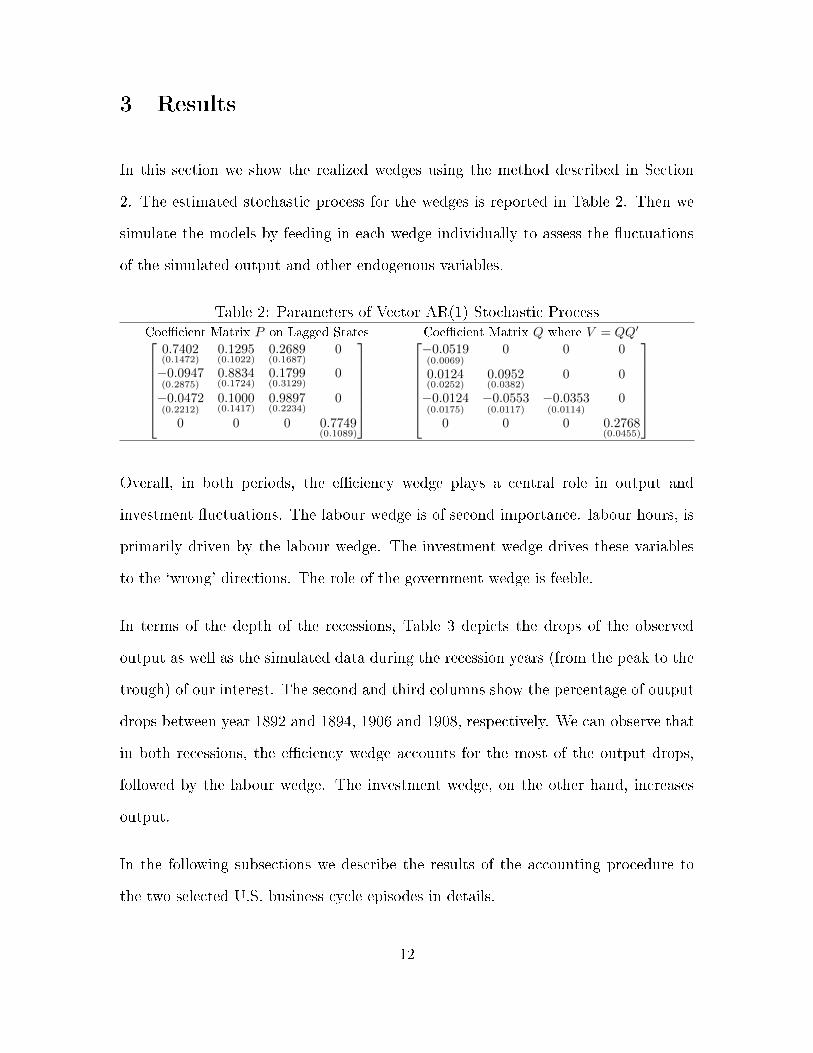
In this section we show the realized wedges using the method described in Section

2. The estimated stochastic process for the wedges is reported in Table 2. Then we

simulate the models by feeding in each wedge individually to assess the �uctuations

of the simulated output and other endogenous variables.

Table 2: Parameters of Vector AR(1) Stochastic ProcessCoe�cient Matrix P on Lagged States Coe�cient Matrix Q where V = QQ′

0.7402(0.1472)

0.1295(0.1022)

0.2689(0.1687)

0

−0.0947(0.2875)

0.8834(0.1724)

0.1799(0.3129)

0

−0.0472(0.2212)

0.1000(0.1417)

0.9897(0.2234)

0

0 0 0 0.7749(0.1089)

−0.0519(0.0069)

0 0 0

0.0124(0.0252)

0.0952(0.0382)

0 0

−0.0124(0.0175)

−0.0553(0.0117)

−0.0353(0.0114)

0

0 0 0 0.2768(0.0455)

Overall, in both periods, the e�ciency wedge plays a central role in output and

investment �uctuations. The labour wedge is of second importance. labour hours, is

primarily driven by the labour wedge. The investment wedge drives these variables

to the `wrong' directions. The role of the government wedge is feeble.

In terms of the depth of the recessions, Table 3 depicts the drops of the observed

output as well as the simulated data during the recession years (from the peak to the

trough) of our interest. The second and third columns show the percentage of output

drops between year 1892 and 1894, 1906 and 1908, respectively. We can observe that

in both recessions, the e�ciency wedge accounts for the most of the output drops,

followed by the labour wedge. The investment wedge, on the other hand, increases

output.

In the following subsections we describe the results of the accounting procedure to

the two selected U.S. business cycle episodes in details.

12

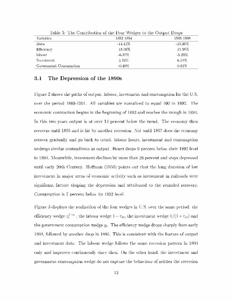
Table 3: The Contribution of the Four Wedges to the Output DropsVariables 1892-1894 1906-1908

Data -14.41% -13.36%

E�ciency -13.55% -15.38%

labour -6.37% -5.29%

Investment 5.76% 6.51%

Government Consumption -0.20% 0.91%

3.1 The Depression of the 1890s

Figure 2 shows the paths of output, labour, investment and consumption for the U.S.

over the period 1889-1901. All variables are nomalized to equal 100 in 1892. The

economic contraction begins in the beginning of 1893 and reaches the trough in 1894.

In this two years output is at over 14 percent below the trend. The economy then

recovers until 1895 and is hit by another recession. Not until 1897 does the economy

recover gradually and go back to trend. labour hours, investment and consumption

undergo similar unsteadiness as output. Hours drops 9 percent below their 1892 level

in 1894. Meanwhile, investment declines by more than 28 percent and stays depressed

until early 20th Century. Ho�man (1956) points out that the long duration of low

investment in major areas of economic activity such as investment in railroads were

signi�cant factors shaping the depression and attributed to the retarded recovery.

Consumption is 7 percent below its 1892 level.

Figure 3 displays the realization of the four wedges in U.S. over the same period: the

e�ciency wedge z1−αt , the labour wedge 1−τht, the investment wedge 1/(1+τxt) and

the government consumption wedge gt. The e�ciency wedge drops sharply from early

1893, followed by another drop in 1895. This is consistent with the feature of output

and investment data. The labour wedge follows the same recession pattern in 1894

only and improves continuously since then. On the other hand, the investment and

government consumption wedge do not capture the behaviour of neither the recession

13

Figure 2: U.S. Output, Labour, Investment and Consumption 1889-1901

1890 1892 1894 1896 1898 1900

70

80

90

100

110

120

OutputLaborInvestmentConsumption

Table 4: Properties of the Wedges 1889-1901

Wedges Standard DeviationCross Correlation

-1 (Lag) 0 1 (Lead)

E�ciency 0.6804 0.0504 0.9446 0.0753

labour 1.0593 0.3571 0.6600 0.3865

Investment 0.9922 -0.1344 -0.7552 -0.1458

Government Consumption 4.8531 0.1969 0.2925 0.5507

nor the recovery during 1889-1901. These relationships are further supported by Table

4 which depicts the standard deviations of the four wedges and their cross correlations

with output. The e�ciency wedge and labour wedge show strong positive correlations

with output whereas the investment wedge is negatively correlated with it. Although

the government consumption wedge is weakly positively correlated with output, its

movement seems to be `too large' relative to the output.

Next, we show decomposition results for output, labour, investment and consump-

tion. Figure 4 to 7 plot the model outcomes of feeding in each wedge individually

or combination of wedges. The �rst panel of these �gures compares the model re-

sults with the e�ciency wedge or labour wedge with data. We can see that there is

14

Figure 3: Measured Wedges, 1889-1901

1890 1892 1894 1896 1898 190085

90

95

100

105

110

115

Efficiency WedgeLabor Wedge

1890 1892 1894 1896 1898 190070

80

90

100

110

120

130

140

150

160

Investment WedgeGovernment Consumption Wedge

15

a remarkable coincidence between simulated model with e�ciency wedge and time

path of output. The e�ciency wedge is also important in explaining the movements

of investment, although it predicts an excessive drop from 1892 to 1894 and a faster

recovery since 1897 compared to the observed investment data. By 1894, simulated

investment drops by more than 39 percent while actual investment only drops by 28

percent. The e�ciency wedge plays a less role in driving the movements of labour

hours. On the other hand, it contributes to neither the sharp decline nor the rapid

recovery of consumption.

Now we evaluate the contribution of the labour wedge. The graph of the simulated

output has a similar pattern as the actual output in both the recession and recovery

periods, however the role of the labour wedge is smaller than that of the e�ciency

wedge. For example, the predicted output falls due to the labour wedge is approx-

imately 7.7 percent less than the drop of output data in 1894. With regards to its

contribution to labour hours, by 1894, the model with the labour wedge completely

replicates the behaviour of labour: it predicts a 9 percent decline in labour, which is

almost the same as the change in the observed labour data. We conclude that it is

the major culprit for the declining labour hours in recession and is also responsible

for its recovery. The arti�cial model predicts a decline in investment from 1892 to

1894, followed by another drop in 1895, but it underestimated the actual drop of

investment. The labour wedge plays no role in consumption.

The second panel of Figures 4 to 7 exposits the contribution of the investment wedge

and the government consumption wedge on variables interested. As shown in these

graphs, the observed and the predicted output and labour hours incorporating each

of these two wedges move in opposite directions. In particular, both wedges fail to

explain the downturn and recovery of the economy. Whereas the investment wedge

16

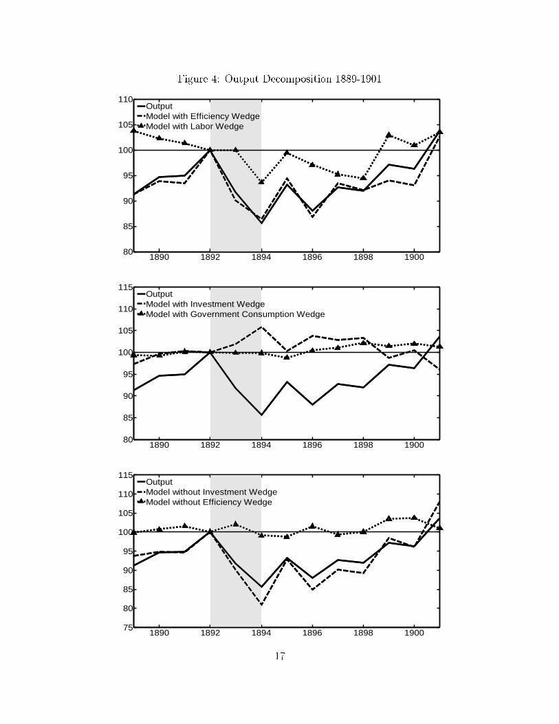
Figure 4: Output Decomposition 1889-1901

1890 1892 1894 1896 1898 190080

85

90

95

100

105

110

OutputModel with Efficiency WedgeModel with Labor Wedge

1890 1892 1894 1896 1898 190080

85

90

95

100

105

110

115

OutputModel with Investment WedgeModel with Government Consumption Wedge

1890 1892 1894 1896 1898 190075

80

85

90

95

100

105

110

115

OutputModel without Investment WedgeModel without Efficiency Wedge

17

Figure 5: Labour Decomposition 1889-1901

1890 1892 1894 1896 1898 190085

90

95

100

105

110

LaborModel with Efficiency WedgeModel with Labor Wedge

1890 1892 1894 1896 1898 190090

95

100

105

110

115

LaborModel with Investment WedgeModel with Government Consumption Wedge

1890 1892 1894 1896 1898 190080

85

90

95

100

105

110

LaborModel without Investment WedgeModel without Efficiency Wedge

18

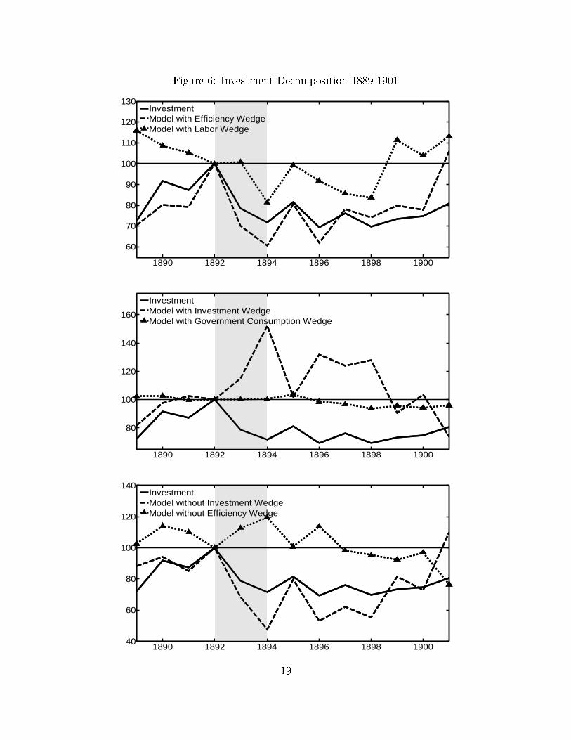
Figure 6: Investment Decomposition 1889-1901

1890 1892 1894 1896 1898 1900

60

70

80

90

100

110

120

130

InvestmentModel with Efficiency WedgeModel with Labor Wedge

1890 1892 1894 1896 1898 1900

80

100

120

140

160

InvestmentModel with Investment WedgeModel with Government Consumption Wedge

1890 1892 1894 1896 1898 190040

60

80

100

120

140

InvestmentModel without Investment WedgeModel without Efficiency Wedge

19

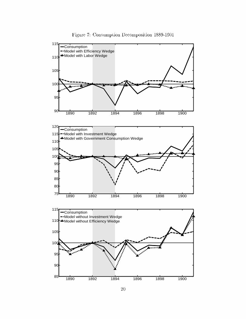
Figure 7: Consumption Decomposition 1889-1901

1890 1892 1894 1896 1898 190090

95

100

105

110

115

ConsumptionModel with Efficiency WedgeModel with Labor Wedge

1890 1892 1894 1896 1898 190075

80

85

90

95

100

105

110

115

120

ConsumptionModel with Investment WedgeModel with Government Consumption Wedge

1890 1892 1894 1896 1898 190085

90

95

100

105

110

115

ConsumptionModel without Investment WedgeModel without Efficiency Wedge

20

plays an important role in the �uctuations of consumption since the model with

investment wedge replicates the development of consumption. Notably, it almost

completely accounts for the recovery of consumption in 1895.

The third panel displays the contribution of the joint wedges which 1) show that the

distortions that manifest themselves as investment wedges are not determinants of the

�uctuations of most variables but consumption. and 2) demonstrates the importance

of the e�ciency wedge on output, labour and investment. As shown in the graphs, the

e�ciency wedge, labour wedge and government consumption wedge together accounts

for almost all of the �uctuations in output. Moreover, if we feed in all of the wedges

except e�ciency wedge into the prototype model, only simulated consumption data

is on the right track.

3.2 The 1907 Recession

We apply the same accounting procedure over the period of 1901-1913. We set 1906

as the base year; therefore all variables are scaled to equal 100 in 1906. In Figure 8,

we can observe that output decreases by more than 13 percent from 1906 to 1908.

At the same time, labour and investment fall drastically as well. It is followed by a

quick but incomplete recovery, and the economy is still around 5 percent below the

trend in 1913.

Figure 9 exposits that the e�ciency wedge has similar movement patterns as output

and investment in both recession and incomplete recovery periods. It is more than

10 percent below the trend in 1908 and remains 7 percent below the trend in 1913.

The condition of the labour wedge also deteriorates due to the `panic' in 1907, but

it improves and surpasses the trend line since then. The behaviour of the govern-

21

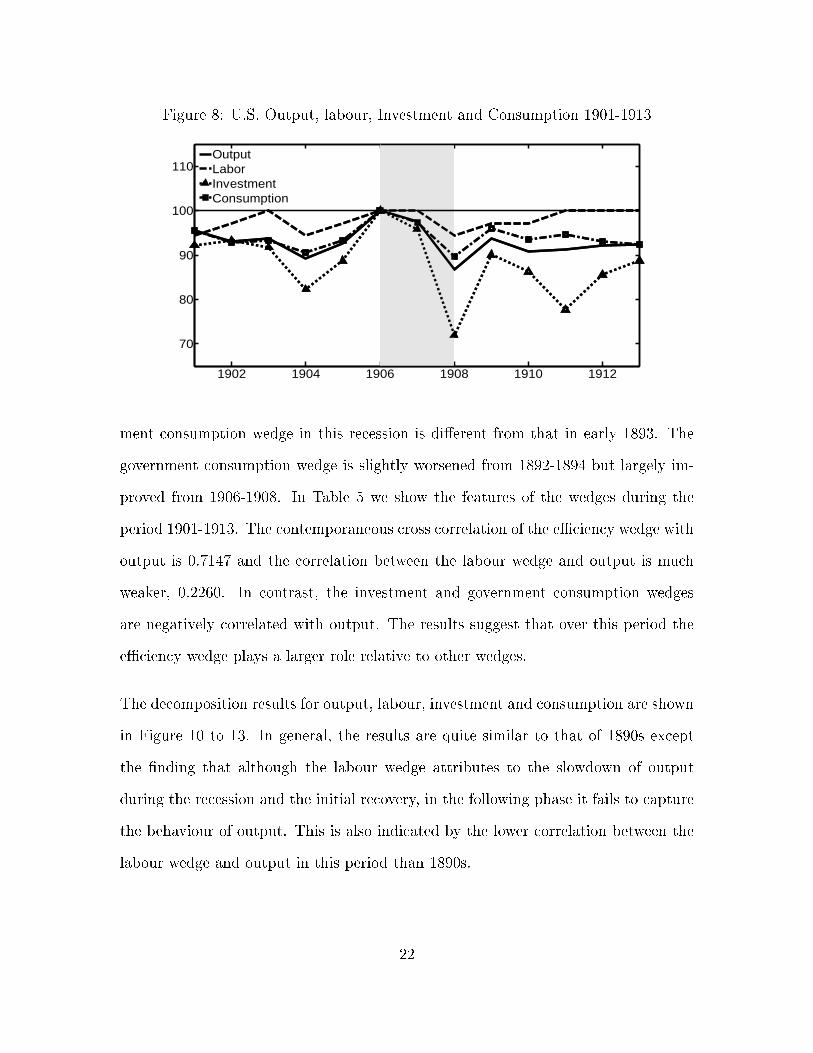
Figure 8: U.S. Output, labour, Investment and Consumption 1901-1913

1902 1904 1906 1908 1910 1912

70

80

90

100

110

OutputLaborInvestmentConsumption

ment consumption wedge in this recession is di�erent from that in early 1893. The

government consumption wedge is slightly worsened from 1892-1894 but largely im-

proved from 1906-1908. In Table 5 we show the features of the wedges during the

period 1901-1913. The contemporaneous cross correlation of the e�ciency wedge with

output is 0.7147 and the correlation between the labour wedge and output is much

weaker, 0.2260. In contrast, the investment and government consumption wedges

are negatively correlated with output. The results suggest that over this period the

e�ciency wedge plays a larger role relative to other wedges.

The decomposition results for output, labour, investment and consumption are shown

in Figure 10 to 13. In general, the results are quite similar to that of 1890s except

the �nding that although the labour wedge attributes to the slowdown of output

during the recession and the initial recovery, in the following phase it fails to capture

the behaviour of output. This is also indicated by the lower correlation between the

labour wedge and output in this period than 1890s.

22

Figure 9: Measured Wedges, 1901-1913

1902 1904 1906 1908 1910 191285

90

95

100

105

110

Efficiency WedgeLabor Wedge

1902 1904 1906 1908 1910 191280

85

90

95

100

105

110

115

120

125

Investment WedgeGovernment Consumption Wedge

Table 5: Properties of the Wedges 1901-1913

Wedges Standard DeviationCross Correlation

-1 (Lag) 0 1 (Lead)

E�ciency 1.3295 0.0863 0.7147 0.1368

labour 1.0080 -0.1950 0.2260 -0.2071

Investment 1.0824 -0.0015 -0.6667 -0.1119

Government Consumption 3.0201 0.3902 -0.1634 -0.0021

23

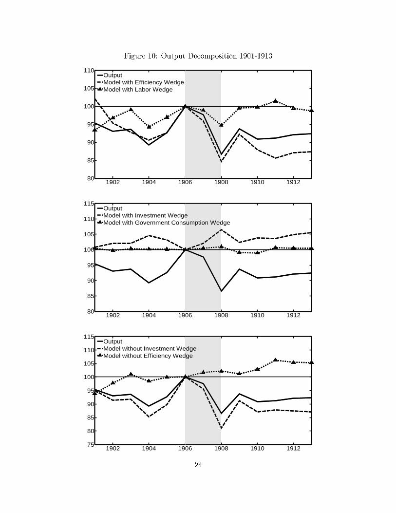
Figure 10: Output Decomposition 1901-1913

1902 1904 1906 1908 1910 191280

85

90

95

100

105

110

OutputModel with Efficiency WedgeModel with Labor Wedge

1902 1904 1906 1908 1910 191280

85

90

95

100

105

110

115

OutputModel with Investment WedgeModel with Government Consumption Wedge

1902 1904 1906 1908 1910 191275

80

85

90

95

100

105

110

115

OutputModel without Investment WedgeModel without Efficiency Wedge

24

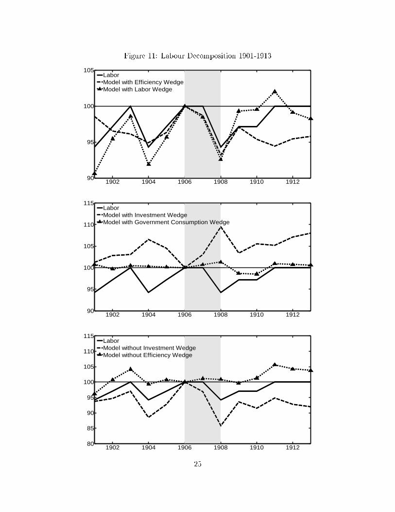
Figure 11: Labour Decomposition 1901-1913

1902 1904 1906 1908 1910 191290

95

100

105

LaborModel with Efficiency WedgeModel with Labor Wedge

1902 1904 1906 1908 1910 191290

95

100

105

110

115

LaborModel with Investment WedgeModel with Government Consumption Wedge

1902 1904 1906 1908 1910 191280

85

90

95

100

105

110

115

LaborModel without Investment WedgeModel without Efficiency Wedge

25

Figure 12: Investment Decomposition 1901-1913

1902 1904 1906 1908 1910 191250

60

70

80

90

100

110

InvestmentModel with Efficiency WedgeModel with Labor Wedge

1902 1904 1906 1908 1910 1912

80

100

120

140

160

180

InvestmentModel with Investment WedgeModel with Government Consumption Wedge

1902 1904 1906 1908 1910 191240

60

80

100

120

140

InvestmentModel without Investment WedgeModel without Efficiency Wedge

26

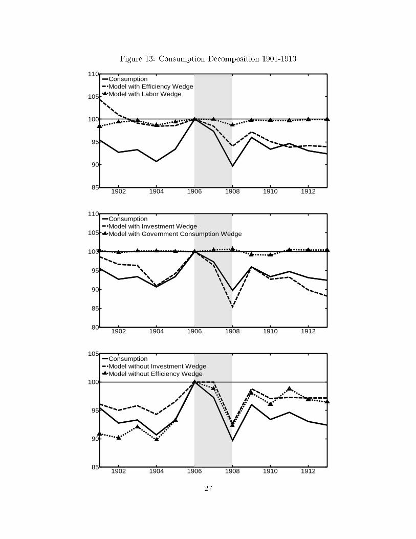
Figure 13: Consumption Decomposition 1901-1913

1902 1904 1906 1908 1910 191285

90

95

100

105

110

ConsumptionModel with Efficiency WedgeModel with Labor Wedge

1902 1904 1906 1908 1910 191280

85

90

95

100

105

110

ConsumptionModel with Investment WedgeModel with Government Consumption Wedge

1902 1904 1906 1908 1910 191285

90

95

100

105

ConsumptionModel without Investment WedgeModel without Efficiency Wedge

27

4 Discussion

The �ndings in the previous section indicate that the �uctuations of output and

investment are primarily driven by the e�ciency wedge. The variation in labour

hours mainly appear from the labour wedge. The investment wedge only accounts for

the movements of consumption. Although none of the wedges could be safely ignored,

the e�ciency and labour wedges are of most importance in explaining the economic

�uctuations compared to other wedges in both sub-periods. In this section we go one

step further to understand what frictions are captured by these wedges and why they

deteriorate during the recessions. More speci�cally, we materialize these wedges in

terms of various macroeconomic variables.

4.1 Understanding the E�ciency Wedge

The Business Cycle Accounting results highlight the contribution of the e�ciency

wedge in economic �uctuations during the pre-1914 period. So what are the prim-

itives that might have caused the deteriorations of the e�ciency wedge during the

recessions?

The e�ciency wedge captures frictions in production. A shift in the aggregate tech-

nology could be one important source of such production deviation. In our benchmark

model, the e�ciency wedge z1−αt is de�ned in a way such that

log(zt) = [log(yt)− αlog(kt)− (1− α)log(ht)]/(1− α),

where the capital utilization rate is assumed to be constant over time. This is es-

sentially the measure of Solow residuals. Whereas, there is abundant evidence that

capital utilization vary signi�cantly over time. Harrison and Weder (2009) stress

28

that procyclical capital utilization could be an important transmission mechanism

of business �uctuations, motivated by Bresnahan and Ra� (1991) �nding that more

than 20 percent of capital stock was idle in 1933. This implies that the Solow resid-

ual measure of production e�ciency tends to overstate the aggregate productivity

�uctuations. Moreover, Burnside, Eichenbaum and Rebelo (1995) argue that cyclical

movement in capital utilization is an important determinant of movement in the total

factor productivity (TFP). Therefore, it is necessary to isolate the e�ect of variable

capital utilization from the e�ciency wedge if one aims to understand the behaviour

of the `true' productivity and the frictions that captured by the e�ciency wedge.

As capital utilization data is not directly available for pre-WWI period, we need to

construct this data series making use of the capital utilization data from 1967 to

1983 and the de�nition of the capacity utilization rate: the ratio of actual output

to the potential output. The source of actual and potential output data from 1889

to 1983 is Hall and Gordon (1986). Capital utilization data is obtained from the

Board of Governors of the Federal Reserve System database. We estimate the simple

linear relationship between the capital utilization rate and actual-potential output

ratio using ordinary least squares estimation. Then we use this relation to infer the

capital utilization rate prior to 1967. Figure 14 compares the observed and estimated

utilization rate over 1967-1983. Figure 15 plots the constructed capital utilization

series {ut} along with output, indicating that the capital utilization rate is procyclical

and strongly correlated with the movements in output. We can also observe in Figure

15 that the �uctuations of capital utilization also coincide with that of the e�ciency

wedge.

29

Figure 14: Capital Utilization during 1967-1983

1968 1970 1972 1974 1976 1978 1980 198270

75

80

85

90

Capital Utilization DataConstructed Capital Utilization

Once we construct the capital utilization rate, we can separate it from the e�ciency

wedge to obtain a new series for total factor productivity using

(z′t)1−α =

z1−αt

uαt,

where (z′t)1−α is the measure of the utilization adjusted productivity. Figure 16 plots

the e�ciency wedge, the adjusted TFP and the Kendrick's (1956) measured TFP

series. The movement of the adjusted TFP is smaller than the measured e�ciency

wedge, indicating that the role of the TFP is exaggerated without considering the

factor hoarding. This is consistent with Chari, Kehoe and McGrattan (2007), Klein

and Otsu (2013) �nding that the variable capital utilization speci�cation downplays

the importance of the e�ciency wedge. Moreover, as can be seen from Figure 16,

the Solow residual, the utilization adjusted and Kendrick's measure of TFP arrive at

similar results.2

2Kendrick's measure is based on a linear production function. Then the TFP index is the weightedarithmetic mean of capital and labour input indices.

30

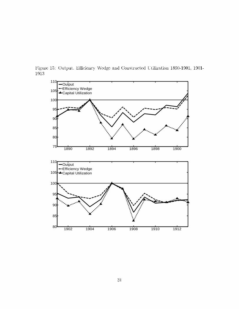
Figure 15: Output, E�ciency Wedge and Constructed Utilization 1890-1901, 1901-1913

1890 1892 1894 1896 1898 190075

80

85

90

95

100

105

110

OutputEfficiency WedgeCapital Utilization

1902 1904 1906 1908 1910 191280

85

90

95

100

105

110

OutputEfficiency WedgeCapital Utilization

31

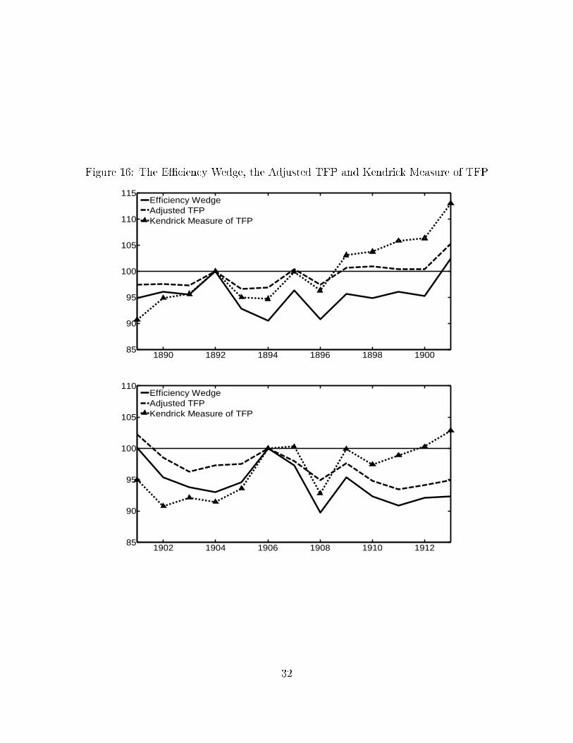
Figure 16: The E�ciency Wedge, the Adjusted TFP and Kendrick Measure of TFP

1890 1892 1894 1896 1898 190085

90

95

100

105

110

115

Efficiency WedgeAdjusted TFPKendrick Measure of TFP

1902 1904 1906 1908 1910 191285

90

95

100

105

110

Efficiency WedgeAdjusted TFPKendrick Measure of TFP

32

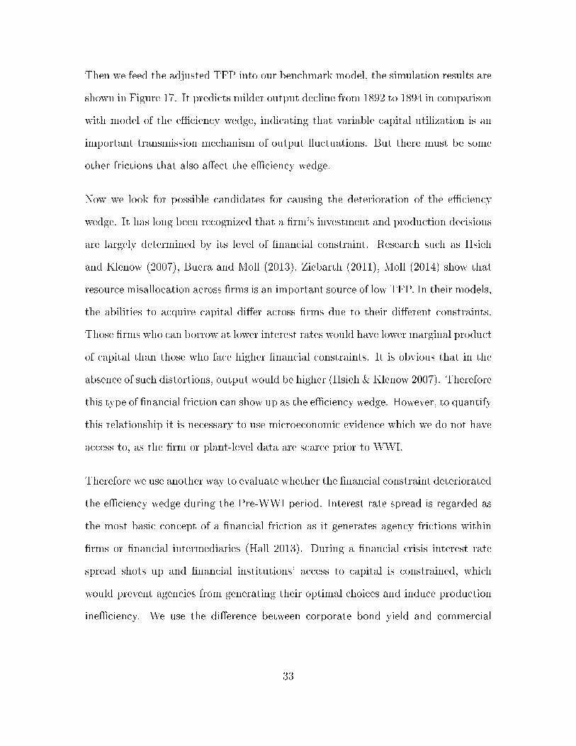
Then we feed the adjusted TFP into our benchmark model, the simulation results are

shown in Figure 17. It predicts milder output decline from 1892 to 1894 in comparison

with model of the e�ciency wedge, indicating that variable capital utilization is an

important transmission mechanism of output �uctuations. But there must be some

other frictions that also a�ect the e�ciency wedge.

Now we look for possible candidates for causing the deterioration of the e�ciency

wedge. It has long been recognized that a �rm's investment and production decisions

are largely determined by its level of �nancial constraint. Research such as Hsieh

and Klenow (2007), Buera and Moll (2013), Ziebarth (2011), Moll (2014) show that

resource misallocation across �rms is an important source of low TFP. In their models,

the abilities to acquire capital di�er across �rms due to their di�erent constraints.

Those �rms who can borrow at lower interest rates would have lower marginal product

of capital than those who face higher �nancial constraints. It is obvious that in the

absence of such distortions, output would be higher (Hsieh & Klenow 2007). Therefore

this type of �nancial friction can show up as the e�ciency wedge. However, to quantify

this relationship it is necessary to use microeconomic evidence which we do not have

access to, as the �rm or plant-level data are scarce prior to WWI.

Therefore we use another way to evaluate whether the �nancial constraint deteriorated

the e�ciency wedge during the Pre-WWI period. Interest rate spread is regarded as

the most basic concept of a �nancial friction as it generates agency frictions within

�rms or �nancial intermediaries (Hall 2013). During a �nancial crisis interest rate

spread shots up and �nancial institutions' access to capital is constrained, which

would prevent agencies from generating their optimal choices and induce production

ine�ciency. We use the di�erence between corporate bond yield and commercial

33

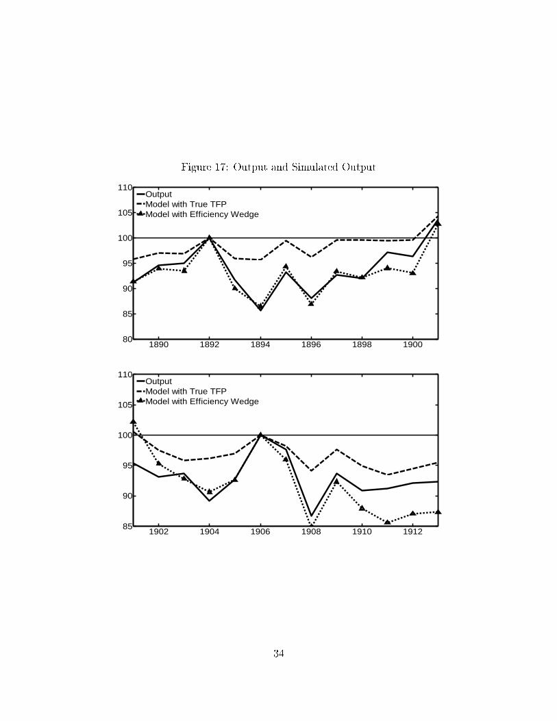
Figure 17: Output and Simulated Output

1890 1892 1894 1896 1898 190080

85

90

95

100

105

110

OutputModel with True TFPModel with Efficiency Wedge

1902 1904 1906 1908 1910 191285

90

95

100

105

110

OutputModel with True TFPModel with Efficiency Wedge

34

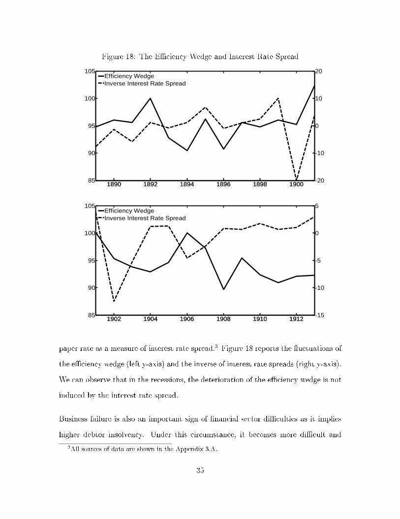
Figure 18: The E�ciency Wedge and Interest Rate Spread

1890 1892 1894 1896 1898 190085

90

95

100

105

1890 1892 1894 1896 1898 1900-20

-10

0

10

20Efficiency WedgeInverse Interest Rate Spread

1902 1904 1906 1908 1910 191285

90

95

100

105

1902 1904 1906 1908 1910 1912-15

-10

-5

0

5Efficiency WedgeInverse Interest Rate Spread

paper rate as a measure of interest rate spread.3 Figure 18 reports the �uctuations of

the e�ciency wedge (left y-axis) and the inverse of interest rate spreads (right y-axis).

We can observe that in the recessions, the deterioration of the e�ciency wedge is not

induced by the interest rate spread.

Business failure is also an important sign of �nancial sector di�culties as it implies

higher debtor insolvency. Under this circumstance, it becomes more di�cult and

3All sources of data are shown in the Appendix 3.A.

35

costly for �rms to obtain credit (Bernanke 1983). Chari, Kehoe and McGrattan (2002)

point out that constraints on input �nancing could generate unpleasant productivity

e�ects. To assess whether the e�ciency wedge was driven by business failure during

1889-1913, we compare this wedge (left y-axis) to the inverse of number of business

failures (right y-axis), as shown in Figure 19. We �nd that the economic downturns

coincide with large business failures.

Both of the 1890s and 1907 economic slumps were associated with bank runs and

�nancial stress. Since the middle of the ninetieth century, railroad and building con-

struction had been two major areas of investment. Investors �owed into these markets

and borrowed too much relying on easy credit, which eventually led to railroad over-

expanding and dried up the capital streams.

�The declining role of the railroad was, indeed, the most signi�cant single

fact for this period and o�ers the most convincing explanation for the

chronic hard times, particularly of the decade of the nineties.� (Fel 1959,

p.73).

The failure in major railroads in 1893 led to a stock market collapse which brought

on pessimism and bank runs.

The panic happened again in 1907. The failure of F. Augustus Heinze's stock ma-

nipulation scheme to corner the stock of United Copper Company led to the collapse

of the share price of the United Copper Company. A bank run was triggered by the

announcement that the National Bank of Commerce would not act as a clearing agent

for Knickerboker Trust Company as the president was reported to have been involved

in Heinze's copper corner. The U.S. banking system over 1863-1913 was character-

36

ized as `the National Banking Era' during which time it had no central bank and no

uniform national currency, re�ecting the weakness of the U.S. banking structure.

Carlson (2005) reports that there were approximately 575 bank failures in the panic

of 1893, and that, in the panic of 1907, clearing houses in 73 cities underwent cash

payment suspension resulting from the bank runs. These constitute major �nancial

market disruptions. Ho�mann (1956) points out that the disruptions of the �nancial

market during the 1890s are the worst among any other depression except that of

1929.

Furthermore, the Sherman Silver Purchase Act mandated that the Federal Reserve

had to purchase increasing amounts of silver each month, which intensi�ed the public

panic due to the belief that the U.S. would not be able to maintain a gold standard

of payments.

In both recessions, banking panic and �nancial crisis resulted in the further shortage

of investment opportunities and curtailing capital accumulation.

Crucini and Kahn (1996) emphasize the importance of tari�s in economic activity.

They argue that substantial material inputs are imported and therefore tari�s can re-

sults in production distortions. In their 2003 paper they demonstrate that increases in

tari�s in a three-sector open economy could manifest themselves as e�ciency wedges

in the prototype model. Therefore we test the role of tari�s on the e�ciency wedge

in our two sample periods. We use the inverse of custom duties data (right y-axis),

shown in Figure 19.4 We can observe that most of the time the inverse tari�s and

the measured TFP move in opposite directions. Most notably the tari�s decline dra-

matically in 1894 and 1908; this tends to increase the productivity and output so the

4The data series is detrended.

37

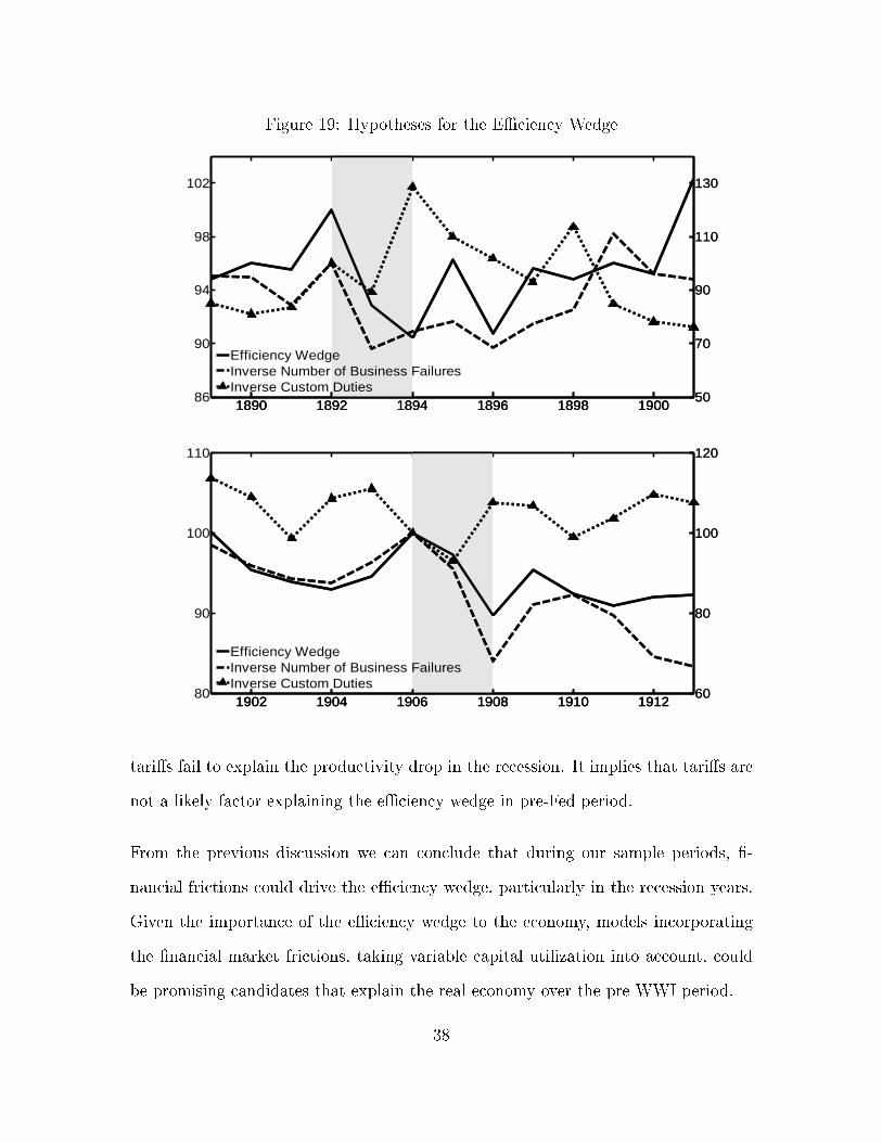
Figure 19: Hypotheses for the E�ciency Wedge

1890 1892 1894 1896 1898 190086

90

94

98

102

1890 1892 1894 1896 1898 190050

70

90

110

130

Efficiency WedgeInverse Number of Business FailuresInverse Custom Duties1890 1892 1894 1896 1898 1900

50

70

90

110

130

1902 1904 1906 1908 1910 191280

90

100

110

1902 1904 1906 1908 1910 191260

80

100

120

Efficiency WedgeInverse Number of Business FailuresInverse Custom Duties1902 1904 1906 1908 1910 1912

60

80

100

120

tari�s fail to explain the productivity drop in the recession. It implies that tari�s are

not a likely factor explaining the e�ciency wedge in pre-Fed period.

From the previous discussion we can conclude that during our sample periods, �-

nancial frictions could drive the e�ciency wedge, particularly in the recession years.

Given the importance of the e�ciency wedge to the economy, models incorporating

the �nancial market frictions, taking variable capital utilization into account, could

be promising candidates that explain the real economy over the pre-WWI period.

38

4.2 Understanding the Labour Wedge

In a perfect competitive market where both households and �rms take wages as given,

competitive equilibrium conditions imply that the marginal rate of substitution equals

the marginal product of labour. However in reality the MRS always deviates from the

MPL. Shimer (2009) de�nes the ratio of the MRS and MPL as the `labour wedge', as

indicated in equation (1). Any deviations from this ratio of 1 indicate that there are

distortions in the labour market.

Now we evaluate factors that may account for the variations in the labour wedge. Gali,

Gertler and Lopez-Salido (2007) and Karabarbounis (2014) decompose the labour

wedge into two components, the wage markup and the price markup. The wage

markup represents the household side of the labour wedge and is captured by the

ratio of the real wage and the MRS. The price markup stands for the fractions in

the labour demand side and is denoted as the ratio of the MPL5 and the real wage.

These markups distort the labour market and therefore are inversely related to the

labour wedge. Figure 20 reports the �uctuations of the labour wedge, the inverse of

wage markup and the inverse of price markup. In accord with previous literatures,

the inverse wage markup explains the most variations of the labour wedge.

Table 6 provides the second moment for output, the labour wedge and the markups

over the period of 1889 to 1913 as a further evidence of the importance of the wage

markup. The wage markup is strongly negatively correlated with both output and

the labour wedge, implying that the �uctuations of output and the labour wedge

are associated with the countercyclical wage markup. On the other hand, the price

markup is much less volatile as the labour wedge and weakly correlated with output

5MRS = θct1−ht

, MPL = (1− α) ytht.

39

Figure 20: Labour Wedge, Inverse of Wage Markup and Inverse of Price Markup

1890 1892 1894 1896 1898 190080

85

90

95

100

105

110

115

120

Labor WedgeInverse Wage MarkupInverse Price Markup

1902 1904 1906 1908 1910 191285

90

95

100

105

110

115

Labor WedgeInverse Wage MarkupInverse Price Markup

40

Table 6: Second Moments 1889-1913

Variable Standard DeviationCross Correlation

Output labour Wedge Wage Markup Price Markup

Output 5.4546 1

labour Wedge 9.0829 0.7680 1

Wage Markup 8.4230 -0.7861 -0.8160 1

Price Markup 4.8708 0.0010 -0.2685 -0.3133 1

and the labour wedge. These �ndings suggest us to focus on the labour supply side

(consumer side) to explain the labour wedge.

Shimer (2009) points out that the most obvious explanation for the reduction of

the labour wedge is the rise of labour and consumption taxes, as it directly a�ects

consumer's decision about the time allocation and labour supply. However, income

tax was not imposed during 1872-1913, except in 1895.

We use the exercise tax as the proxy of the consumption tax since the data of other

types of consumption tax are not available. The inverse consumption tax is shown

in Figure 23. We don't observe the feature that higher consumption tax induces

lower labour wedge. Therefore, taxes do not a�ect the labour wedge much during the

pre-1914 period.

Another explanation claims that the monetary shocks would a�ect the labour wedge.

More speci�cally, prices changes induced by monetary shocks would a�ect the econ-

omy through intertemporal substitution of leisure and unexpected wage changes (Lu-

cas & Rapping 1969).

We evaluate the impact of the monetary shocks on the labour wedge during the Na-

tional Banking Era. Bernanke (1995) points out that banking panic leads to increases

in currency-deposit ratio which is negatively related to money multiplier. Therefore

we use the U.S. money multiplier as a measure of the monetary disturbance. The

41

multiplier is represented as the ratio of aggregate broad money (M2) over base money

(M0). Figure 23 illustrates that the movement patterns of the money multiplier is

quite similar to that of the labour wedge, especially for the �rst sample period. It

displays a dramatic decline in the money multiplier in both recession years, implying

that it could be a convenient explanation as it coincides with the decline of the labour

wedge.

During the National Banking Era not only state banks but also some large non-

�nancial institutions such as railroad and bridge companies were allowed to issue their

own banknotes. Any unpleasant news would hit depositors and investors, creating

con�dence shock. Once such pessimistic expectations exceeded a certain threshold,

bank runs occur, causing signi�cant declines in money supply. Eventually, the deep

recession was triggered and the MRS fell o� sharply. Because the National Banking

Era was a period where there were no `lenders of last resort', there was no reliable

way to expand the money supply.

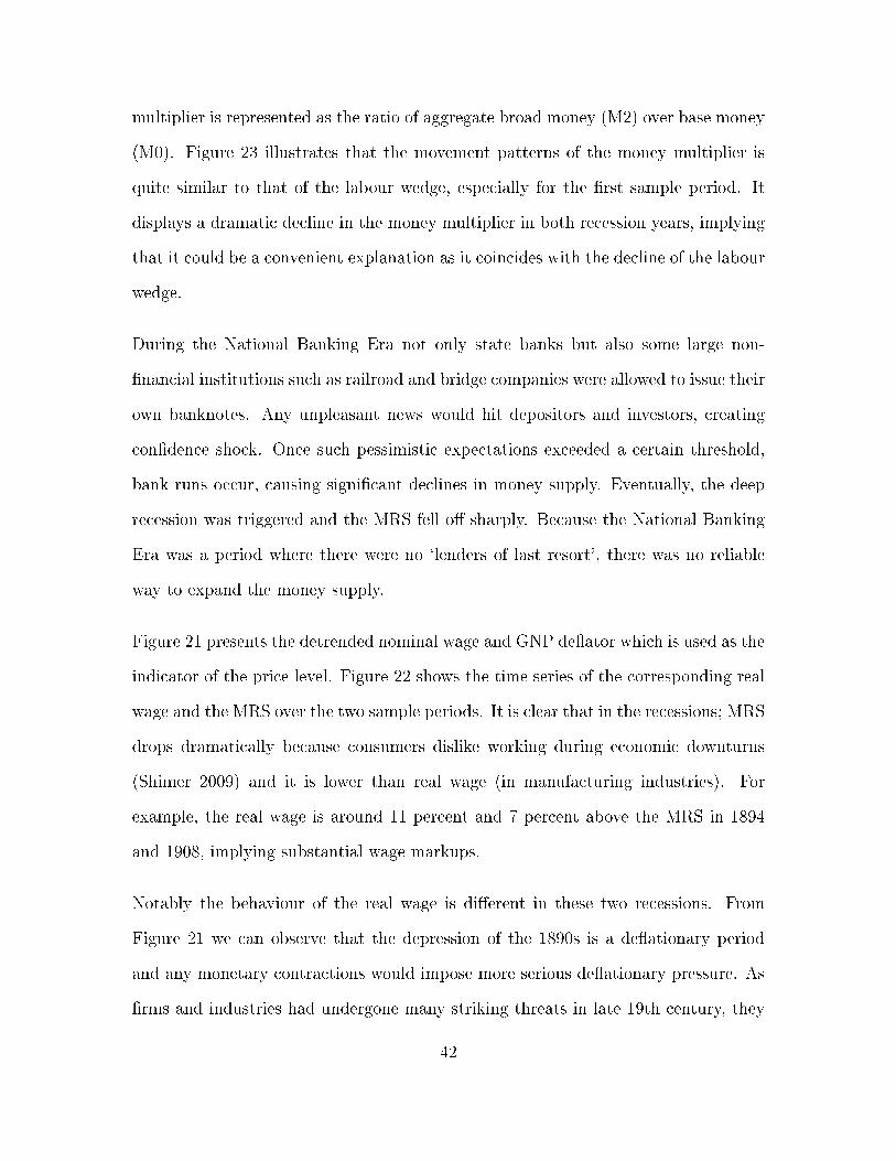
Figure 21 presents the detrended nominal wage and GNP de�ator which is used as the

indicator of the price level. Figure 22 shows the time series of the corresponding real

wage and the MRS over the two sample periods. It is clear that in the recessions; MRS

drops dramatically because consumers dislike working during economic downturns

(Shimer 2009) and it is lower than real wage (in manufacturing industries). For

example, the real wage is around 11 percent and 7 percent above the MRS in 1894

and 1908, implying substantial wage markups.

Notably the behaviour of the real wage is di�erent in these two recessions. From

Figure 21 we can observe that the depression of the 1890s is a de�ationary period

and any monetary contractions would impose more serious de�ationary pressure. As

�rms and industries had undergone many striking threats in late 19th century, they

42

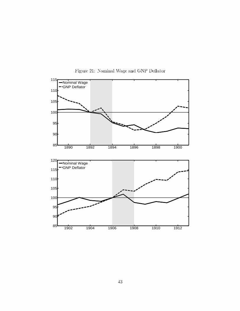
Figure 21: Nominal Wage and GNP De�ator

1890 1892 1894 1896 1898 190085

90

95

100

105

110

115

Nominal WageGNP Deflator

1902 1904 1906 1908 1910 191285

90

95

100

105

110

115

120

Nominal WageGNP Deflator

43

Figure 22: Real Wage and MRS

1890 1892 1894 1896 1898 190085

90

95

100

105

110

115

Real WageMRS

1902 1904 1906 1908 1910 191285

90

95

100

105

110

115

Real WageMRS

44

were unlikely to cut the nominal wages (Hanes 1993). Sundstrom (1992) also stresses

that workers' resistance to reduce their wage was one culprit of the sluggishness of

nominal wage adjustment in the 1892-1894 recession. One of the most outstanding

strikes was the May Day strike of 1886. Therefore over this period the nominal wage

is relatively sticky compared to the falling price. Real wage slightly declined before it

increases in 1893. This induce a huge gap between the real wage and the MRS. For

this period, the wage stickness intensi�es the e�ects of the negative monetary shock

on the labour wedge.

On the other hand, during the period of 1901 to 1913, prices show a persistent upward

trend, which could be the result of increasing gold stock (Friedman & Schwartz 1963).

Moreover, Figure 22 shows very di�erent behaviour of the real wage in 1901-1913

compared with the previous decade. Particularly, during the 1906-1908 downturn the

real wage decreases instead of increasing. The real wage is declined as a result of the

rise in in�ation and the relative stickness of the nominal wage.

Cole and Ohanian (2004) emphasize that the cartelization and labour unions could

result in markups over the competitive wage. We use union membership as a measure

of the strength of the labour unions. Stronger labour bargaining power allows workers

to increase their wage above the market-clearing level (Cole & Ohanian 2002) and

therefore worsen the labour wedge. Figure 23 displays the �uctuations of the inverse

of union membership. It may partly explain the �uctuations of the labour wedge for

some periods, particularly for 1892-1894. Moreover, the slight decline of the strength

of the labour union from 1907 coincides with the failure of the 1907 Mesabi Range

Strike. The Mesabi Range Strike was the �rst organized strike on the Iron Range,

motivated by dangerous working conditions and low wages. This unsuccessful strike

was mainly due to the strikebreakers hired by the Oliver Iron Mining Company.

45

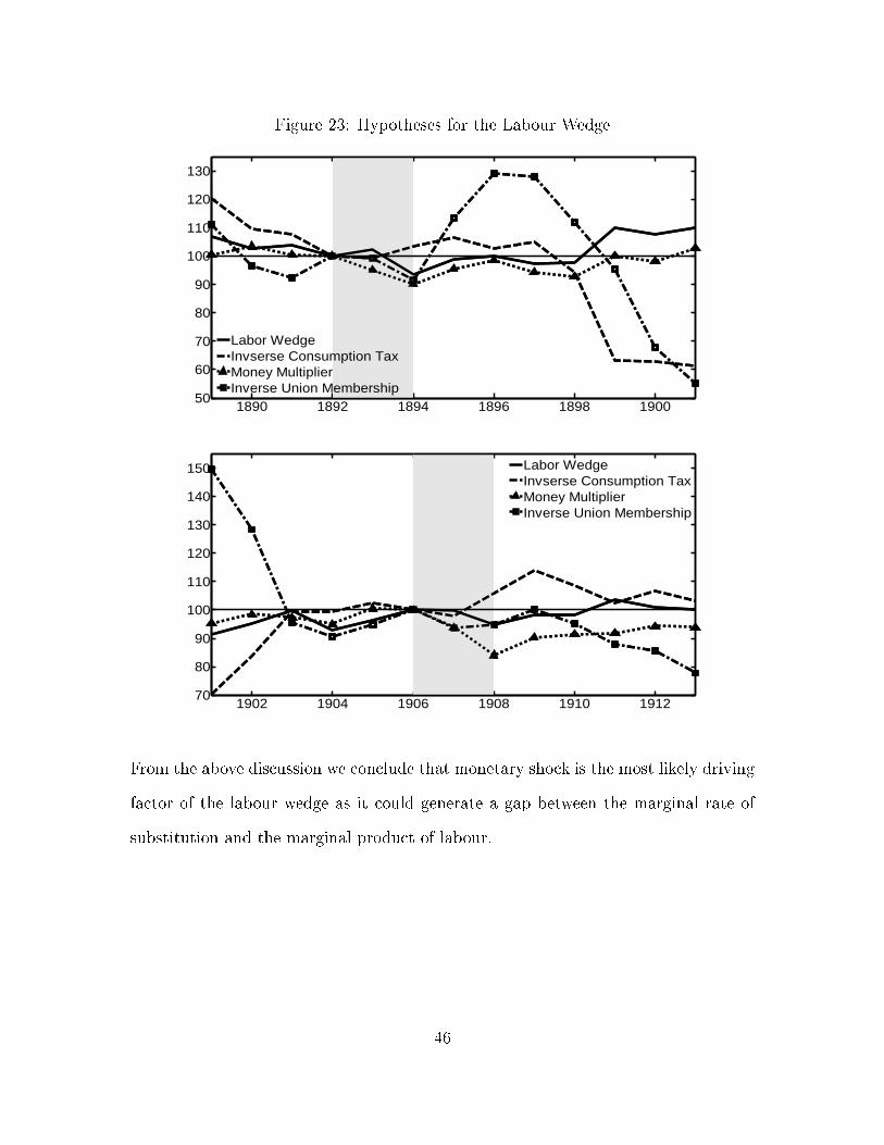
Figure 23: Hypotheses for the Labour Wedge

1890 1892 1894 1896 1898 190050

60

70

80

90

100

110

120

130

Labor WedgeInvserse Consumption TaxMoney MultiplierInverse Union Membership

1902 1904 1906 1908 1910 191270

80

90

100

110

120

130

140

150

Labor WedgeInvserse Consumption TaxMoney MultiplierInverse Union Membership

From the above discussion we conclude that monetary shock is the most likely driving

factor of the labour wedge as it could generate a gap between the marginal rate of

substitution and the marginal product of labour.

46

5 Conclusion

We conduct the Business Cycle Accounting exercises on U.S. data for the cyclical

episode from 1889 to 1901 and from 1901 to 1913 to �gure out the distortions that

are primarily responsible for the economic �uctuations, particularly the 1893 and

1907 recessions. We �nd that the e�ciency wedge alone almost accounts for the �uc-

tuations of output and investment, and the labour wedge plays a secondary role. The

movement of hours is mainly a�ected by the labour market frictions. The investment

and government consumption wedge drive these variables to the `wrong' directions.

The BCA approach provides useful insight for researchers as it aims to �nd out the

channel for the transmission of shocks to the economy and therefore allows them

to identify the promising class of theories investigating the pre-WWI period. Our

results imply that any models attempting to replicate the economic behaviour of

this period should consider the market frictions that could manifest themselves as

the e�ciency wedge and the labour wedge in the prototype model. We compare the

measured e�ciency wedge with number of business failures and, �nd that �nancial

market frictions may be a possible candidate that deteriorate the e�ciency wedge.

To understand the labour market frictions, we need to focus on the demand side of

labour, that is, the discrepancy in the MRS and the real wage. Our results show that

it could be attributed to the monetary shocks.

47

Appendix A Data Sources

This Appendix provides the details of source and construction of the data used in

this paper. All data are annually for the period 1889-1913 unless otherwise stated.

A.1 Original Data

O.1. Gross National Product, Commerce Concept. Millions of 1929 Dollars. Source:

Kendrick (1956), P.290, Table A-IIa.

O.2. Gross National Product, Commerce Concept. Millions of Current Dollars.

Source: Kendrick (1956), P.296, Table A-IIb.

O.3. Manhours, Total. Millions. Source: Kendrick (1956), P.311, Table A-X.

O.4. Total Consumption Expenditures, Commerce Concept. Billions of 1929 Dollars.

Source: Kendrick (1956), P.290, Table A-IIa.

O.5. Gross Private Domestic Investment, Commerce Concept. Millions of 1929 Dol-

lars. Source: Kendrick (1956). P.290, Table A-IIa.

O.6. Consumption Durables. Millions of Current Dollars. Source: Historical Statis-

tics of the United States (2006), P.3-270, Series Cd411.

O.7. Resident Population, Total. Thousand. Source: Historical Statistics of the

United States (2006), P.1-28, Series Aa7.

O.8. Capital Utilization Rate. 1967-1983. Source: Board of Governors of the Federal

Reserve System Database, G17.

48

O.9. Real Gross National Product. 1972 Dollars. Source: Hall and Gordon (1986),

P.781, Table 1.

O.10. Trend Real Gross National Product. 1972 Dollars. Source; Hall and Gordon

(1986), P.781, Table 1.

O.11. Stock Price Index. Source: Cowles (1939), Common Stock Indexes.

O.12. Custom Duties. Thousand Dollars. Source: Annual Report of the Secretary of

the Treasury, 1929, P.428.

O.13. Exercise Taxes. Thousand Dollars. Source: Historical Statistics of the United

States, Colonial Times to 1970, p.1108, Series 364-373.

O.14. Aggregate Broad Money M2, Friedman and Schwartz. Source: Historical

Statistics of the United States (2006), P.3-604, Series Cj45.

O.15. High-Powered Money M0. Source: Historical Statistics of the United States

(2006), P.3-631, Series Cj141.

O.16. Nominal Hourly Earnings, Manufacturing. Source: Historical Statistics of the

United States (2006), P.2-270, Series Ba4314.

O.17. Union Members, Friedman. Thousand. Source: Historical Statistics of the

United States (2006), P.2-336, Series Ba4789.

O.18. Total Factor Productivity, Commerce Concept. Source: Kendrick (1956), Table

A-XXII.

O.19. Yield on Corporate Bonds. Source: Hall and Gordon (1986), p.781, Table 1.

O.20. Commercial Paper Rate. Source: Hall and Gordon (1986), p.781, Table 1.

49

O.21. Number of Business Failures. Source: Historical Statistics of the United States

(2006), P.3-550, Series Ch411.

A.2 Constructed Data

C.1. GNP De�ator=O.2./O.1.

C.2. Net Factor Payments=0.005×O.1.

C.3. Real Per Capita Output=O.1./O.7./1000

C.4. Real Per Capita Investment=(O.5.+O.6./C.1.+C.2.)/O.7./1000

C.5. Real Per Capita Consumption=(O.4.×1000 - O.6/C.1.)/O.7./1000

C.6. Per Capita Hours Worked=O.3./O.7./1000

C.7. Real Custom Duties=O.12./C.1.

C.8. Real Exercise Taxes=O.13./C.1.

C.9. Money Multiplier=O.14./O.15.

C.10. Capacity Utilization=O.9./O.10.

C.11. Real Wage=O.16./C.1.

C.12. Interest Rate Spread = O.19. - O.20.

References

[1] Bemanke, B. S., 1995. The macroeconomics of the Great Depression: a compar-

ative approach. Journal of Money, Credit, and Banking 27 (1), 1�28.

50

[2] Bernanke, B. S., Gertler, M., Gilchrist, S., 1999. The �nancial accelerator in a

quantitative business cycle framework. Handbook of macroeconomics 1, 1341�

1393.

[3] Bresnahan, T. F., Ra�, D. M., 1991. Intra-industry heterogeneity and the Great

Depression: the American motor vehicles industry, 1929�1935. The Journal of

Economic History 51 (02), 317�331.

[4] Buera, F. J., Moll, B., 2012. Aggregate implications of a credit crunch. National

Bureau of Economic Research Working Paper (17775).

[5] Carlson, M., 2005. Causes of bank suspensions in the panic of 1893. Explorations

in Economic History 42 (1), 56�80.

[6] Carter, S. B., Gartner, S. S., Haines, M. R., Olmstead, A. L., Sutch, R., Wright,

G., 2006. Historical statistics of the United States. Cambridge University Press,

New York.

[7] Chari, V. V., Kehoe, P. J., McGrattan, E. R., 2002. Accounting for the Great

Depression. American Economic Review 92 (2), 22�27.

[8] Chari, V. V., Kehoe, P. J., McGrattan, E. R., 2007. Business cycle accounting.

Econometrica 75 (3), 781�836.

[9] Cole, H. L., Ohanian, L. E., 2002. The US and UK Great Depressions through

the lens of neoclassical growth theory. American Economic Review 92 (2), 28�32.

[10] Cole, H. L., Ohanian, L. E., 2004. New Deal policies and the persistence of the

Great Depression: a general equilibrium analysis. Journal of Political Economy

112 (4), 779�816.

51

[11] Crucini, M. J., Kahn, J., 1996. Tari�s and aggregate economic activity: lessons

from the Great Depression. Journal of Monetary Economics 38 (3), 427�467.

[12] Crucini, M. J., Kahn, J. A., 2003. Tari�s and the Great Depression revisited.

Federal Reserve Bank of New York Sta� Reports (172).

[13] Fels, R., 1959. American business cycles, 1865-1897. University of North Carolina

Press, Chapel Hill.

[14] Gali, J., Gertler, M., Lopez-Salido, J. D., 2007. Markups, gaps, and the welfare

costs of business �uctuations. The Review of Economics and Statistics 89 (1),

44�59.

[15] Hall, R. E., Gordon, R. J., 1986. The American business cycle: continuity and

change. University of Chicago Press, Chicago.

[16] Hanes, C., 1993. The development of nominal wage rigidity in the late 19th

century. The American Economic Review 83 (4), 732�756.

[17] Harrison, S., Weder, M., 2009. Technological change and the roaring Twenties:

a neoclassical perspective. Journal of Macroeconomics 31 (3), 363�375.

[18] Ho�mann, C., 1956. The depression of the nineties. The Journal of Economic

History 16 (2), 137�164.

[19] Hsieh, C.-T., Klenow, P. J., 2007. Misallocation and manufacturing TFP in

China and India. National Bureau of Economic Research Working Paper (13290).

[20] Karabarbounis, L., 2014. The labor wedge: MRS vs. MPN. Review of Economic

Dynamics 17 (2), 206�223.

52

[21] Kendrick, J., 1956. Productivity trends: capital and labor. National Bureau of

Economic Research.

[22] Klein, A., Otsu, K., 2013. E�ciency, distortions and factor utilization during the

interwar period. University of Kent School of Economics Discussion Papers.

[23] Lucas, R. E., Rapping, L. A., 1969. Real wages, employment, and in�ation. The

Journal of Political Economy 77 (5), 721�754.

[24] Shimer, R., 2009. Convergence in macroeconomics: the labor wedge. American

Economic Journal: Macroeconomics 1 (1), 280�297.

[25] Sundstrom, W. A., 1992. Rigid wages or small equilibrium adjustments? Evi-

dence from the contraction of 1893. Explorations in Economic History 29 (4),

430�455.

[26] Ziebarth, N., 2011. Misallocation and productivity during the Great Depression.

Northwestern University Mimeo.

53