Embed Size (px)
Citation preview
User & Documentation Manual BCE TRANSIT 1.0 – 09/2015
BusinessCaseEvaluatorA Value and Risk Based Enhancement to EnvisionTM
TRANSIT MODULE

Written By
Ben Rommelaere, John Parker and Ryan Meyers
Impact Infrastructure, Inc
Designed By
Dvorak Design, Ltd
Published by Impact Infrastructure, Inc., New York, New York – Copyright © 2015Published simultaneously in Canada.
Licensed to the Institute for Sustainable Infrastructure (ISI) for use by its members through 2016 subject to renewal.
Limit of Liability/ Disclaimer of Warranty: While the publisher and author have used their best efforts in preparing this manual, they make no representations or warranties with respect to the accuracy or completeness of the contents of this book and associated spreadsheets and specifically disclaim any implied warranties of merchant ability or fitness for a particular purpose.
For more information contact: www.impactinfrastructure.com/contact/
Created by Impact Infrastructure, Inc. with input from members of the ISI Economics Committee BCE TRANSIT 1.0 – 09/2015
WALK-THROUGH INTRODUCTION..........................................................................................................1Introduction................................................................................................................................................................................1
Model Inputs ...............................................................................................................................................................................2
Input Risk Ranges ........................................................................................................................................................................3
Conventions and Navigation.............................................................................................................................................................4
Spreadsheet Conventions and Navigation .....................................................................................................................................4
Opening the Excel Workbook ........................................................................................................................................................4
PART I – INPUTS PAGES .....................................................................................................................................................................5Page 1 (“Location and Dates”) ...........................................................................................................................................................................................5Page 2 (“Transit & Auto Information”) ...............................................................................................................................................................................5Page 3 (“Emissions Information”) ......................................................................................................................................................................................6Page 4 (“Active Transportation”) ........................................................................................................................................................................................7Page 5 (“Land Use Characteristics”) ...................................................................................................................................................................................7Page 6 (“CapEx and O&M Costs”) .......................................................................................................................................................................................7Page 7 (“Revenue”)............................................................................................................................................................................................................9Page 8 (“Subsidies, Decommissioning, & Other”) ..............................................................................................................................................................9Page 9 (“Tree Planting & Removal”) ..................................................................................................................................................................................9
PART II: USER-DEFINED MODEL INPUTS .............................................................................................................................................10Advanced User Inputs ......................................................................................................................................................................................................10
PART III: RESULTS ...........................................................................................................................................................................11Page 1 – Monte Carlo Simulation (“Results – Monte Carlo Simulation”) .........................................................................................................................11Page 2 – Summary (“Results – Summary – Risk Adjusted”) ...........................................................................................................................................11Page 3 – Static Projections (“Results – Static Projections”) .............................................................................................................................................11Page 4 – Multiple Stakeholder Accounts Analysis (“Multiple Account Costs & Benefits”) ................................................................................................12Page 5 – Envision Credits Allocation (“Envision Credit Costs & Benefits”) ........................................................................................................................13
DESCRIPTION OF ECONOMIC BENEFITS AND APPROACH TO VALUATION....................................................14Economic Valuation Approach..........................................................................................................................................................................................14BCE Links to EnvisionTM Credits .........................................................................................................................................................................................14Valuation Methods ..........................................................................................................................................................................................................15Risk Analysis Approach ....................................................................................................................................................................................................15Social Discount Rate ........................................................................................................................................................................................................15Use of EnvisionTM Business Case Evaluator ........................................................................................................................................................................16Transit Type Descriptions & Definitions ............................................................................................................................................................................17Economic Benefits ...........................................................................................................................................................................................................18Increases Revenues and Avoided Costs ............................................................................................................................................................................19Value of Travel Time Savings ............................................................................................................................................................................................20
The Value of Travel Time Savings .................................................................................................................................................................................20The Value of Congestion ..............................................................................................................................................................................................26
Value of Reliability ...........................................................................................................................................................................................................30Measuring Reliability ..................................................................................................................................................................................................30Theoretical Models of VOR...........................................................................................................................................................................................31Empirical Estimations of the Value of Reliability (VOR)................................................................................................................................................31
Low Income Mobility Benefit ...........................................................................................................................................................................................35Ownership – Vehicle Operating Costs ...............................................................................................................................................................................38
Contents
iiENVISIONTM TRANSIT BUSINESS CASE EVALUATOR DOCUMENTATION
iiiENVISIONTM TRANSIT BUSINESS CASE EVALUATOR DOCUMENTATION
Contents
Ownership – Fixed Vehicle Costs ......................................................................................................................................................................................39Reduced Accident Risk Benefit .........................................................................................................................................................................................40
Value of Statistical Life ................................................................................................................................................................................................41Air Pollution & CO2 Emissions Reduction..........................................................................................................................................................................42Noise Pollution Reduction ................................................................................................................................................................................................44Oil Consumption Externality.............................................................................................................................................................................................46Avoided Road Facilities Costs ............................................................................................................................................................................................48Personal & Social Value of Active Transportation ..............................................................................................................................................................49Perception of Safety Benefit .............................................................................................................................................................................................51Property Value Uplift ........................................................................................................................................................................................................52Shadow Wage Benefit ......................................................................................................................................................................................................54After Tax Wage Transfer & Income Tax Transfer..................................................................................................................................................................55
RESULTS AND OUTPUTS OF THE BUSINESS CASE EVALUATOR.................................................................................................................56Monte Carlo Simulation ...................................................................................................................................................................................................56Results Summary.............................................................................................................................................................................................................58Static Results ...................................................................................................................................................................................................................58Multiple Account Costs and Benefits................................................................................................................................................................................59EnvisionTM Credit Costs and Benefits.................................................................................................................................................................................60
APPENDICES ....................................................................................................................................61Appendix A – BCE Cost and Benefits to EnvisionTM Credits Mapping ...................................................................................................61
Appendix B – Risk Analysis Approach ..............................................................................................................................................66
Appendix C – Default Values Used in Business Case Evaluator............................................................................................................68Discounting, Inflation, and Tax Rates...........................................................................................................................................................................68Traffic Flow Characteristics ..........................................................................................................................................................................................68Vehicle Types & Mode Choice Assumptions .................................................................................................................................................................69Active Transportation Assumptions.............................................................................................................................................................................69Consumption Multiplier Assumptions .........................................................................................................................................................................70Social Cost of Carbon & Criteria Air Contaminants .......................................................................................................................................................70New Trees....................................................................................................................................................................................................................71
Appendix D – Changes to Business Case Evaluator Default Values For Philadelphia Stormwater Management Study Comparison..........72
Appendix E – Social Discount Rate...................................................................................................................................................74Social Opportunity Cost of Capital ...............................................................................................................................................................................74Rate of Time Preference ..............................................................................................................................................................................................75Social Discount Rate and Sustainability.......................................................................................................................................................................75From the U.S. EPA:.......................................................................................................................................................................................................76International Comparisons..........................................................................................................................................................................................77Social Discount Rate Conclusion ..................................................................................................................................................................................77
Appendix F – Optional Inputs .........................................................................................................................................................78
ENVISIONTM TRANSIT BUSINESS CASE EVALUATOR DOCUMENTATION
Contents
BUSINESS CASE EVALUATOR REFERENCES................................................................................................80General .........................................................................................................................................................................................80
The Value of Travel Time Savings.....................................................................................................................................................80
The Value of Congestion .................................................................................................................................................................80
The Value of Reliability ..................................................................................................................................................................81
Low Income Mobility Benefit ..........................................................................................................................................................83
Ownership – Operating Costs..........................................................................................................................................................83
Ownership – Fixed Costs .................................................................................................................................................................83
Reduced Accident Risk Benefit ........................................................................................................................................................84
Value of Statistical Life...................................................................................................................................................................84
Air Pollution and Carbon Emissions Reduction .................................................................................................................................85
Noise Pollution ..............................................................................................................................................................................86
Oil Consumption Externalities.........................................................................................................................................................86
Avoided Road Facilities Costs ..........................................................................................................................................................87
Active Transportation.....................................................................................................................................................................87
Perception of Safety Benefit...........................................................................................................................................................88
Property Value Uplift .....................................................................................................................................................................88
BPR Curves ....................................................................................................................................................................................89
iv
Business Case Evaluator – TransitUser Manual
IntroductionAt Impact Infrastructure we go through a research, prototyping, and development process to develop our cost-benefit decision support tools for in-frastructure projects and their design. After a literature review we build a prototype. This is a fully functioning, stand-alone, cost benefit and riskanalysis model. After testing it internally we ask industry experts to give it a try and then release it as a companion economic tool for the EnvisionTM
sustainable infrastructure rating system. Our first Business Case Evaluator (BCE) was for stormwater management and modelled the benefits ofgreen infrastructure, otherwise known as low impact development (LID) or best management practices (BMP). Our latest BCE is for transit. The Excel model that accompanies this documentation estimates the benefits of transit relative to a base transportation case and can be used toevaluate new transit infrastructure of different types as well as operational improvements in existing transit. We are aware that many such modelshave been created. The problem facing the practitioner is that they are specific to one situation, geography, or are not maintained and updatedwith new data. We aim to correct this with the BCE for Transit. The first version is for the U.S. and as with the Stormwater BCE we will add Canada.Any updates to the excel model and this document, can be downloaded from www.impactinfrastructure.com.
AutoCASE® is the commercial version of the BCE models. It is integrated across infrastructure types, shareable and cloud-based, and avail-able as an extension to Autodesk’s design and planning software tools. AutoCASE benefits from more regular updates and enhancementsthan the BCE models. Impact Infrastructure also supports AutoCASE with training and customization if required. AutoCASE for Transit isgoing to be built into Autodesk's Infraworks 360 design software. By combining AutoCASE's analytics with spatial data we think you will beable to better create, view, analyze, share, and manage information to make decisions in context.
Results in the model are presented as Sustainable Net Present Value (S-NPV) as well as traditional financial NPV. Financial and SustainableReturn on Investment (ROI) and payback periods are also calculated. All results are the product of Monte Carlo simulation and so are pre-sented in probabilistic terms.
In early versions we had a traffic simulator built in but have decided not to include it as we saw the uses of AutoCASE being using the output from amicro-simulation or four-step transportation planning model. Also AutoCASE will be linked to some of the exciting land-use planning and trans-portation simulations in Autodesk. These are truly exciting and will make AutoCASE for Transit a wonderfully rich visual planning and design tool.
Document LayoutThis guide is designed to help users apply the BCE tool to projects, while also explaining the tools capabilities and identifying its limitations. Thesteps needed to run a model have been numbered for your convenience. For the input pages, the numbered steps in this manual correspond to thenumbers for each input on each input page in the Excel worksheets. For the output pages, screenshots have been taken, and the important com-ponents of each screenshot have been surrounded by red boxes and numbered.
Walk-Through Introduction
1ENVISIONTM TRANSIT BUSINESS CASE EVALUATOR DOCUMENTATION
Model InputsIt is important to remember that not all inputs in the BCE need to be filled out in order to run the model.
For most projects, there will likely be several input categories that are not relevant. If this is the case, or the user does not have reliable informa-tion for a specific input, it can be left blank. For example, a change in miles cycled may not be relevant to your project, therefore this input couldbe left blank. As a general rule, the more inputs that are filled out with accurate information, the more reliable the results will be in reflectingthe true costs and benefits of the project.
Required Inputs
Required inputs (can be imported from four stage transportation or micro-simulation model):
n Project location and dates
n Type of Transit
n Does the New Transit Infrastructure Replace Existing Transit Infrastructure?nWhat type of transit infrastructure is being replaced?
n Hour of the day, or just the peak hour?
n Years of Traffic Data Available
n Automobile Traffic Informationn Average Automobile Trip Lengthn Average Peak AM Congested Automobile Speedn Average Free-flow Automobile Speedn Average Vehicle Miles Travelled
n Transit Traffic Informationn Average Transit Travel Timen Average Transit Travel Distancen Average Transit Travel Speedn Peak AM Transit Tripsn Percent of Transit Time Spent in Vehiclesn Percent of Transit Time Spent Walkingn Percent of Transit Time Spent Waitingn Peak Hour Passenger to Capacity Ration Percent of Riders Who have a Seat at 100% Capacity during Peak AM Hour
n Transit Hours of Operations (New and Old Service if applicable)nWeekday Transit Operating HoursnWeekend Transit Operating Hoursn Capital Expenditure and Operations and Maintenance Costs (will eventually link to cost estimation databases)n Bureau of Public Roads (BPR) Curve Parameters
The remaining inputs are optional. The list of optional inputs has been provided, for your convenience, in Appendix F.
Walk-Through Introduction
2ENVISIONTM TRANSIT BUSINESS CASE EVALUATOR DOCUMENTATION
Input Risk RangesMost of the inputs include the capability of indicating a low, expected (or most likely), and high value for each variable. These ranges providethe basis for the risk assessment in the model, allowing the user to indicate uncertainty around values. If the user has a specific value for aninput, they can simply enter a value for the “Most Likely Value”, leaving the low and high value boxes blank. In the case that the user has onlylow and most likely values, the high value can be set as equal to the most likely value. Similarly, if the user has only the most likely and high val-ues, the low value can be set as equal to the most likely value.
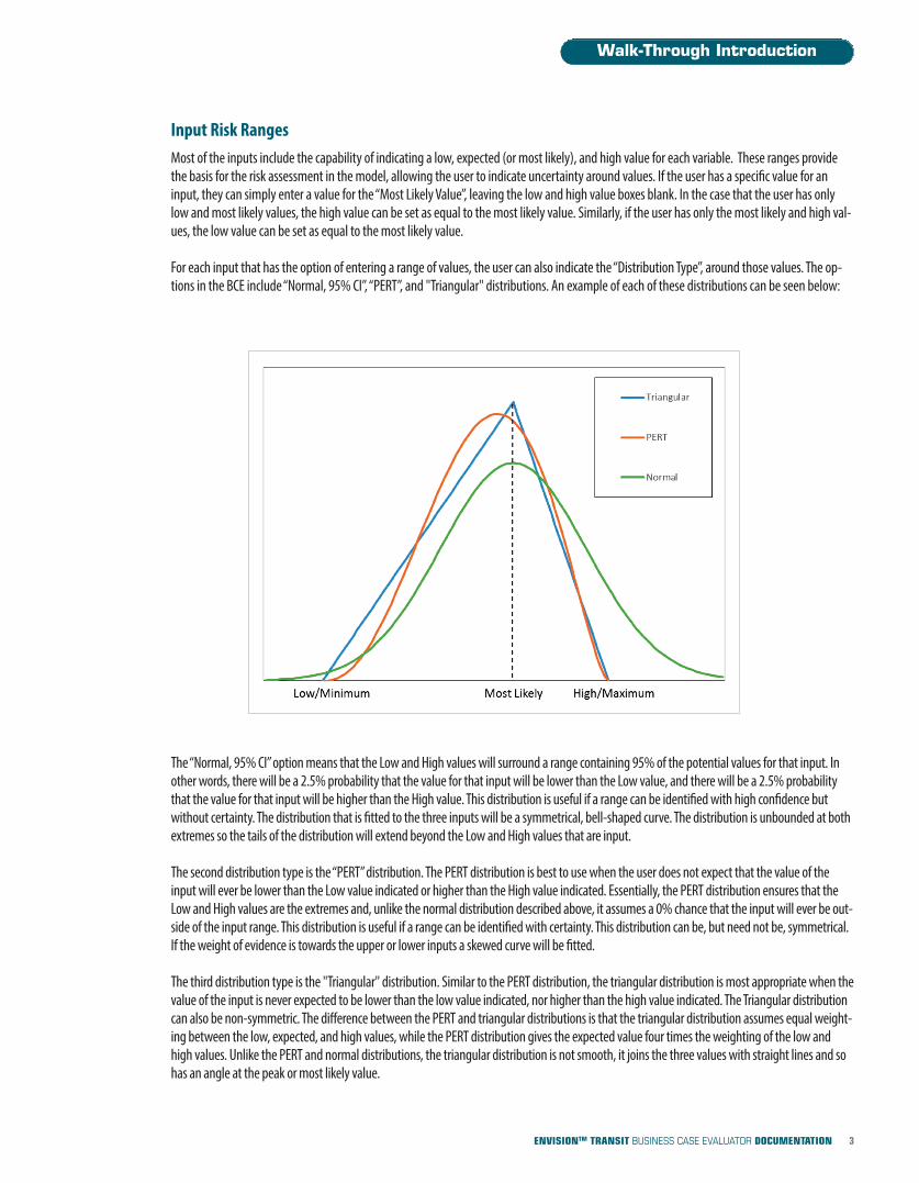
For each input that has the option of entering a range of values, the user can also indicate the “Distribution Type”, around those values. The op-tions in the BCE include “Normal, 95% CI”, “PERT”, and "Triangular" distributions. An example of each of these distributions can be seen below:
The “Normal, 95% CI” option means that the Low and High values will surround a range containing 95% of the potential values for that input. Inother words, there will be a 2.5% probability that the value for that input will be lower than the Low value, and there will be a 2.5% probabilitythat the value for that input will be higher than the High value. This distribution is useful if a range can be identified with high confidence butwithout certainty. The distribution that is fitted to the three inputs will be a symmetrical, bell-shaped curve. The distribution is unbounded at bothextremes so the tails of the distribution will extend beyond the Low and High values that are input.
The second distribution type is the “PERT” distribution. The PERT distribution is best to use when the user does not expect that the value of theinput will ever be lower than the Low value indicated or higher than the High value indicated. Essentially, the PERT distribution ensures that theLow and High values are the extremes and, unlike the normal distribution described above, it assumes a 0% chance that the input will ever be out-side of the input range. This distribution is useful if a range can be identified with certainty. This distribution can be, but need not be, symmetrical.If the weight of evidence is towards the upper or lower inputs a skewed curve will be fitted.
The third distribution type is the "Triangular" distribution. Similar to the PERT distribution, the triangular distribution is most appropriate when thevalue of the input is never expected to be lower than the low value indicated, nor higher than the high value indicated. The Triangular distributioncan also be non-symmetric. The difference between the PERT and triangular distributions is that the triangular distribution assumes equal weight-ing between the low, expected, and high values, while the PERT distribution gives the expected value four times the weighting of the low andhigh values. Unlike the PERT and normal distributions, the triangular distribution is not smooth, it joins the three values with straight lines and sohas an angle at the peak or most likely value.
Walk-Through Introduction
3ENVISIONTM TRANSIT BUSINESS CASE EVALUATOR DOCUMENTATION
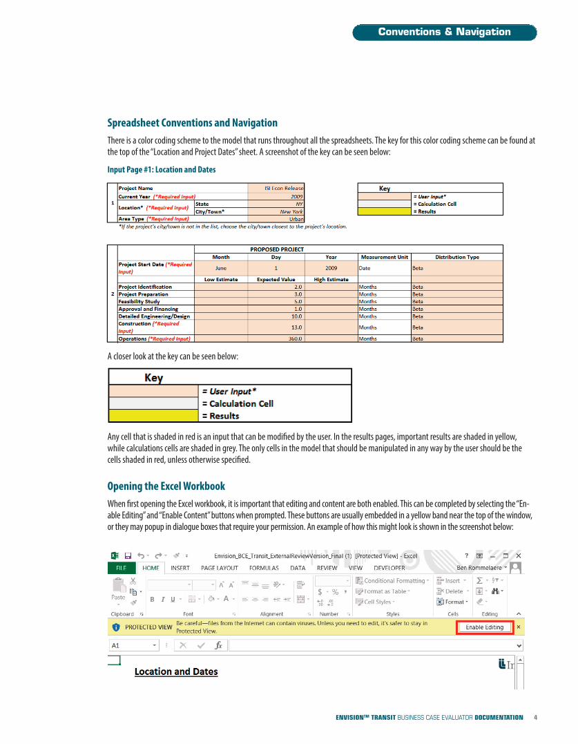
Spreadsheet Conventions and NavigationThere is a color coding scheme to the model that runs throughout all the spreadsheets. The key for this color coding scheme can be found atthe top of the “Location and Project Dates” sheet. A screenshot of the key can be seen below:
Input Page #1: Location and Dates
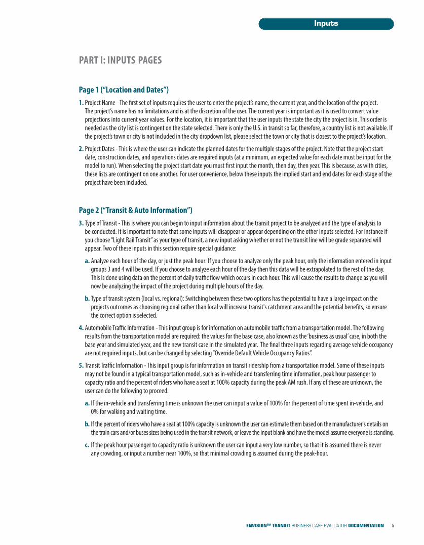
A closer look at the key can be seen below:
Any cell that is shaded in red is an input that can be modified by the user. In the results pages, important results are shaded in yellow, while calculations cells are shaded in grey. The only cells in the model that should be manipulated in any way by the user should be the cells shaded in red, unless otherwise specified.
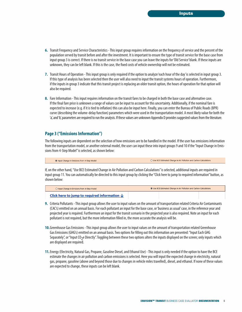
Opening the Excel WorkbookWhen first opening the Excel workbook, it is important that editing and content are both enabled. This can be completed by selecting the “En-able Editing” and “Enable Content” buttons when prompted. These buttons are usually embedded in a yellow band near the top of the window,or they may popup in dialogue boxes that require your permission. An example of how this might look is shown in the screenshot below:
Conventions & Navigation
4ENVISIONTM TRANSIT BUSINESS CASE EVALUATOR DOCUMENTATION
PART I: INPUTS PAGES
Page 1 (“Location and Dates”)1. Project Name - The first set of inputs requires the user to enter the project’s name, the current year, and the location of the project.
The project’s name has no limitations and is at the discretion of the user. The current year is important as it is used to convert value projections into current year values. For the location, it is important that the user inputs the state the city the project is in. This order is needed as the city list is contingent on the state selected. There is only the U.S. in transit so far, therefore, a country list is not available. If the project’s town or city is not included in the city dropdown list, please select the town or city that is closest to the project’s location.
2. Project Dates - This is where the user can indicate the planned dates for the multiple stages of the project. Note that the project start date, construction dates, and operations dates are required inputs (at a minimum, an expected value for each date must be input for the model to run). When selecting the project start date you must first input the month, then day, then year. This is because, as with cities, these lists are contingent on one another. For user convenience, below these inputs the implied start and end dates for each stage of the project have been included.
Page 2 (“Transit & Auto Information”)3. Type of Transit - This is where you can begin to input information about the transit project to be analyzed and the type of analysis to
be conducted. It is important to note that some inputs will disappear or appear depending on the other inputs selected. For instance if you choose “Light Rail Transit” as your type of transit, a new input asking whether or not the transit line will be grade separated will appear. Two of these inputs in this section require special guidance:
a. Analyze each hour of the day, or just the peak hour: If you choose to analyze only the peak hour, only the information entered in input groups 3 and 4 will be used. If you choose to analyze each hour of the day then this data will be extrapolated to the rest of the day. This is done using data on the percent of daily traffic flow which occurs in each hour. This will cause the results to change as you will now be analyzing the impact of the project during multiple hours of the day.
b. Type of transit system (local vs. regional): Switching between these two options has the potential to have a large impact on the projects outcomes as choosing regional rather than local will increase transit's catchment area and the potential benefits, so ensure the correct option is selected.
4. Automobile Traffic Information - This input group is for information on automobile traffic from a transportation model. The following results from the transportation model are required: the values for the base case, also known as the ‘business as usual’ case, in both the base year and simulated year, and the new transit case in the simulated year. The final three inputs regarding average vehicle occupancy are not required inputs, but can be changed by selecting “Override Default Vehicle Occupancy Ratios”.
5. Transit Traffic Information - This input group is for information on transit ridership from a transportation model. Some of these inputs may not be found in a typical transportation model, such as in-vehicle and transferring time information, peak hour passenger to capacity ratio and the percent of riders who have a seat at 100% capacity during the peak AM rush. If any of these are unknown, the user can do the following to proceed:
a. If the in-vehicle and transferring time is unknown the user can input a value of 100% for the percent of time spent in-vehicle, and 0% for walking and waiting time.
b. If the percent of riders who have a seat at 100% capacity is unknown the user can estimate them based on the manufacturer's details on the train cars and/or buses sizes being used in the transit network, or leave the input blank and have the model assume everyone is standing.
c. If the peak hour passenger to capacity ratio is unknown the user can input a very low number, so that it is assumed there is never any crowding, or input a number near 100%, so that minimal crowding is assumed during the peak-hour.
Inputs
5ENVISIONTM TRANSIT BUSINESS CASE EVALUATOR DOCUMENTATION
6. Transit Frequency and Service Characteristics - This input group requires information on the frequency of service and the percent of the population served by transit before and after the investment. It is important to ensure the type of transit service for the base case from input group 3 is correct. If there is no transit service in the base case you can leave the inputs for ‘Old Service’ blank. If these inputs are unknown, they can be left blank. If this is the case, the fixed costs of vehicle ownership will not be estimated.
7. Transit Hours of Operation - This input group is only required if the option to analyze ‘each hour of the day’ is selected in input group 3. If this type of analysis has been selected then the user will also need to input the transit systems hours of operation. Furthermore, if the inputs in group 3 indicate that this transit project is replacing an older transit option, the hours of operation for that option will also be required.
8. Fare Information - This input requires information on the transit fares to be charged in both the base case and alternative case. If the final fare price is unknown a range of values can be input to account for this uncertainty. Additionally, if the nominal fare is expected to increase (e.g. if it is tied to inflation) this can also be input here. Finally, you can enter the Bureau of Public Roads (BPR) curve (describing the volume-delay function) parameters which were used in the transportation model. A most likely value for both the ‘a’, and ‘b’, parameters are required to run the analysis. If these values are unknown Appendix D provides suggested values from the literature.
Page 3 (“Emissions Information”)The following inputs are dependent on the selection of how emissions are to be handled in the model. If the user has emissions informationfrom the transportation model, or another external model, the user can input these into input groups 9 and 10 if the “Input Change in Emis-sions from 4-Step Model” is selected, as shown below:
If, on the other hand, “Use BCE Estimated Change in Air Pollution and Carbon Calculations” is selected, additional inputs are required ininput group 11. You can automatically be directed to this input group by clicking the “Click here to jump to required information” button, asshown below:
9. Criteria Pollutants - This input group allows the user to input values on the amount of transportation related Criteria Air Contaminants (CAC’s) emitted on an annual basis. For each pollutant an input for the base case, or ‘business as usual’ case, in the reference year and projected year is required. Furthermore an input for the transit scenario in the projected year is also required. Note an input for each pollutant is not required, but the more information filled in, the more accurate the analysis will be.
10.Greenhouse Gas Emissions - This input group allows the user to input values on the amount of transportation related Greenhouse Gas Emissions (GHG’s) emitted on an annual basis. Two options for filling out this information are presented: “Input Each GHG Separately”, or “Input CO2e Directly”. Toggling between these two options alters the inputs displayed on the screen; only inputs which are displayed are required.
11. Energy (Electricity, Natural Gas, Propane, Gasoline Diesel, and Ethanol Use) - This input is only needed if the option to have the BCE estimate the changes in air pollution and carbon emissions is selected. Here you will input the expected change in electricity, natural gas, propane, gasoline (above and beyond those due to changes in vehicle miles travelled), diesel, and ethanol. If none of these values are expected to change, these inputs can be left blank.
Inputs
6ENVISIONTM TRANSIT BUSINESS CASE EVALUATOR DOCUMENTATION
Page 4 (“Active Transportation”)12. Active Transportation - This input group allows the user to input information changes in the number of miles cycled and/or the
number of miles walked.
a. It is important to note that for miles walked the input number should be above and beyond the change in walking implied in the transit and auto information on page 2. This is because the change in miles walked due to switching from commuting via automobiles to transit and changes due to changing walking times within the transit system are already accounted for.
Page 5 (“Land Use Characteristics”)13. Pre and Post Project Land Use Characteristics - This input requires the user to input the total amount of concrete required in the
construction of the transit project.
14. Residential and Commercial Property Proximity to Stations - This input group requires information about the properties around the proposed transit stations. The first option is to choose whether or not you want to fill in the detailed information. If “I have detailed information that I will fill in” is selected new input lines will appear and these new lines must be filled in. Alternatively, if “I would like an automatic estimation” is selected, these lines will disappear and will no longer need to be filled in. In either case the last three inputs on the ‘percent of properties within 400, 800, and 1200 meters (approximately 1/4, 1/2, and 3/4 of a mile) that are currently in equal proximity to alternative transit’ should be filled in to ensure the property value model works correctly.
Page 6 (“CapEx and O&M Costs”)Capital expenditure (CapEx) costs must be estimated in order to run a full analysis. If these costs are known (or an estimate is available) they can be entered directly. The following definition of capital costs outlines what costs should be included in these inputs:
“ Capital costs are fixed, one-time expenses incurred on the purchase of land, buildings, construction, and equipment used in the production of goods or in the rendering of services. Put simply, it is the total cost needed to bring a project to a commercially operable status.” [1]
If these costs are unknown, you can input any positive value; if you want to simply measure the benefits of a project, you can enter $1 as a value. If this approach is taken, note that some of the metrics (such as Return on Investment or Discounted Payback Period) may be deceiving, as they are based on a cost of $1.
Capital expenditures are automatically spread out evenly over the construction duration. For example, if capital expenditures are expected to cost $10 million and the dates of construction are as follows:
Start: Jan 1, 2015
Planning Duration: 12 months
Construction Duration: 30 months
Due to the 12 month planning stage, it would be expected that construction would start on Jan 1 2016. Then, because construction is takingplace over 2 ½ years, the first $4 million would be spent in 2016, then $4 million would be spend in 2017, and the final $2 million would bespent in 2018. These values would then be discounted over their respective years and summed to determine the Net Present Value of capitalexpenditures.
Inputs
7ENVISIONTM TRANSIT BUSINESS CASE EVALUATOR DOCUMENTATION
[1] Capital cost from Wikipedia, the free encyclopedia
Inputs
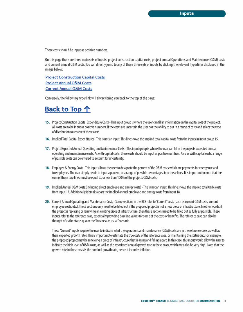
These costs should be input as positive numbers.
On this page there are three main sets of inputs: project construction capital costs, project annual Operations and Maintenance (O&M) costsand current annual O&M costs. You can directly jump to any of these three sets of inputs by clicking the relevant hyperlinks displayed in theimage below:
Conversely, the following hyperlink will always bring you back to the top of the page:
15. Project Construction Capital Expenditure Costs - This input group is where the user can fill in information on the capital cost of the project. All costs are to be input as positive numbers. If the costs are uncertain the user has the ability to put in a range of costs and select the type of distribution to represent these costs.
16. Implied Total Capital Expenditures - This is not an input. This line shows the implied total capital costs from the inputs in input group 15.
17. Project Expected Annual Operating and Maintenance Costs - This input group is where the user can fill in the projects expected annual operating and maintenance costs. As with capital costs, these costs should be input as positive numbers. Also as with capital costs, a range of possible costs can be entered to account for uncertainty.
18. Employee & Energy Costs - This input allows the user to designate the percent of the O&M costs which are payments for energy use and to employees. The user simply needs to input a percent, or a range of possible percentages, into these lines. It is important to note that the sum of these two lines must be equal to, or less than 100% of the projects O&M costs.
19. Implied Annual O&M Costs (including direct employee and energy costs) - This is not an input. This line shows the implied total O&M costs from input 17. Additionally it breaks apart the implied annual employee and energy costs from input 18.
20. Current Annual Operating and Maintenance Costs - Some sections in the BCE refer to “Current” costs (such as current O&M costs, current employee costs, etc.). These sections only need to be filled out if the proposed project is not a new piece of infrastructure. In other words, if the project is replacing or renewing an existing piece of infrastructure, then these sections need to be filled out as fully as possible. These inputs refer to the reference case, essentially providing baseline values for some of the costs or benefits. The reference case can also be thought of as the status quo or the “business as usual” scenario.
These “Current” inputs require the user to indicate what the operations and maintenance (O&M) costs are in the reference case, as well as their expected growth rates. This is important to estimate the true costs of the reference case, or maintaining the status quo. For example, the proposed project may be renewing a piece of infrastructure that is aging and falling apart. In this case, this input would allow the user to indicate the high level of O&M costs, as well as the associated annual growth rate in these costs, which may also be very high. Note that the growth rate in these costs is the nominal growth rate, hence it includes inflation.
8ENVISIONTM TRANSIT BUSINESS CASE EVALUATOR DOCUMENTATION
Inputs
9ENVISIONTM TRANSIT BUSINESS CASE EVALUATOR DOCUMENTATION
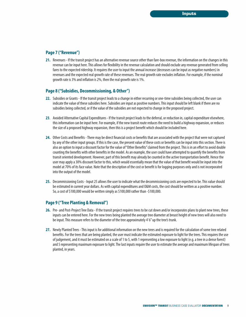
Page 7 (“Revenue”)21. Revenues - If the transit project has an alternative revenue source other than fare-box revenue, the information on the changes in this
revenue can be input here. This allows for flexibility in the revenue calculation and should exclude any revenue generated from selling fares to the expected ridership. It requires the user to input the annual increase (decreases can be input as negative numbers) in revenues and the expected real growth rate of these revenues. The real growth rate excludes inflation. For example, if the nominal growth rate is 3% and inflation is 2%, then the real growth rate is 1%.
Page 8 (“Subsidies, Decommissioning, & Other”)22. Subsidies or Grants - If the transit project leads to a change in either recurring or one-time subsidies being collected, the user can
indicate the value of these subsidies here. Subsidies are input as positive numbers. This input should be left blank if there are no subsidies being collected, or if the value of the subsidies are not expected to change in the proposed project.
23. Avoided Alternative Capital Expenditures - If the transit project leads to the deferral, or reduction in, capital expenditure elsewhere, this information can be input here. For example, if the new transit route reduces the need to build a highway expansion, or reduces the size of a proposed highway expansion, then this is a project benefit which should be included here.
24. Other Costs and Benefits - There may be direct financial costs or benefits that are associated with the project that were not captured by any of the other input groups. If this is the case, the present value of these costs or benefits can be input into this section. There is also an option to input a discount factor for the value of “Other Benefits” claimed from the project. This is in an effort to avoid double counting the benefits with other benefits in the model. As an example, the user could have attempted to quantify the benefits from transit oriented development. However, part of this benefit may already be counted in the active transportation benefit. Hence the user may apply a 30% discount factor to this, which would essentially mean that the value of that benefit would be input into the model at 70% of its face value. Note that the description of the cost or benefit is for logging purposes only and is not incorporated into the output of the model.
25. Decommissioning Costs - Input 25 allows the user to indicate what the decommissioning costs are expected to be. This value should be estimated in current year dollars. As with capital expenditures and O&M costs, the cost should be written as a positive number. So, a cost of $100,000 would be written simply as $100,000 rather than -$100,000.
Page 9 (“Tree Planting & Removal”)26. Pre- and Post-Project Tree Data - If the transit project requires trees to be cut down and/or incorporates plans to plant new trees, these
inputs can be entered here. For the new trees being planted the average tree diameter at breast height of new trees will also need to be input. This measure refers to the diameter of the tree approximately 4’ 6” up the tree’s trunk.
27. Newly Planted Trees - This input is for additional information on the new trees and is required for the calculation of some tree related benefits. For the trees that are being planted, the user must indicate the estimated exposure to light for the trees. This requires the use of judgement, and it must be estimated on a scale of 1 to 5, with 1 representing a low exposure to light (e.g. a tree in a dense forest) and 5 representing maximum exposure to light. The last inputs require the user to estimate the average and maximum lifespan of trees planted, in years.
Inputs
10ENVISIONTM TRANSIT BUSINESS CASE EVALUATOR DOCUMENTATION
PART II: USER-DEFINED MODEL INPUTS
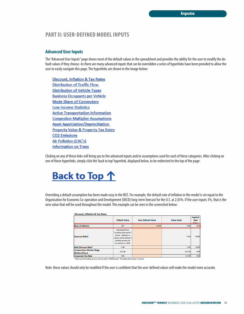
Advanced User InputsThe “Advanced User Inputs” page shows most of the default values in the spreadsheet and provides the ability for the user to modify the de-fault values if they choose. As there are many advanced inputs that can be overridden a series of hyperlinks have been provided to allow theuser to easily navigate this page. The hyperlinks are shown in the image below:
Clicking on any of these links will bring you to the advanced inputs and/or assumptions used for each of these categories. After clicking onone of these hyperlinks, simply click the ‘back to top’ hyperlink, displayed below, to be redirected to the top of the page:
Overriding a default assumption has been made easy in the BCE. For example, the default rate of inflation in the model is set equal to theOrganisation for Economic Co-operation and Development (OECD) long-term forecast for the U.S. at 2.03%. If the user inputs 3%, that is thenew value that will be used throughout the model. This example can be seen in the screenshot below:
Note: these values should only be modified if the user is confident that the user-defined values will make the model more accurate.
11ENVISIONTM TRANSIT BUSINESS CASE EVALUATOR DOCUMENTATION
PART III: RESULTS
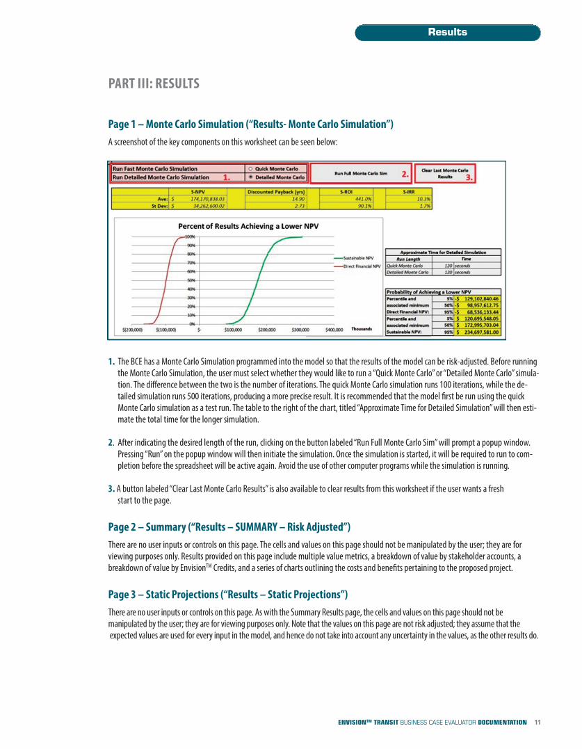
Page 1 – Monte Carlo Simulation (“Results- Monte Carlo Simulation”)A screenshot of the key components on this worksheet can be seen below:
1. The BCE has a Monte Carlo Simulation programmed into the model so that the results of the model can be risk-adjusted. Before runningthe Monte Carlo Simulation, the user must select whether they would like to run a “Quick Monte Carlo” or “Detailed Monte Carlo” simula-tion. The difference between the two is the number of iterations. The quick Monte Carlo simulation runs 100 iterations, while the de-tailed simulation runs 500 iterations, producing a more precise result. It is recommended that the model first be run using the quickMonte Carlo simulation as a test run. The table to the right of the chart, titled “Approximate Time for Detailed Simulation” will then esti-mate the total time for the longer simulation.
2. After indicating the desired length of the run, clicking on the button labeled “Run Full Monte Carlo Sim” will prompt a popup window.Pressing “Run” on the popup window will then initiate the simulation. Once the simulation is started, it will be required to run to com-pletion before the spreadsheet will be active again. Avoid the use of other computer programs while the simulation is running.
3. A button labeled “Clear Last Monte Carlo Results” is also available to clear results from this worksheet if the user wants a fresh start to the page.
Page 2 – Summary (“Results – SUMMARY – Risk Adjusted”)There are no user inputs or controls on this page. The cells and values on this page should not be manipulated by the user; they are for viewing purposes only. Results provided on this page include multiple value metrics, a breakdown of value by stakeholder accounts, abreakdown of value by EnvisionTM Credits, and a series of charts outlining the costs and benefits pertaining to the proposed project.
Page 3 – Static Projections (“Results – Static Projections”)There are no user inputs or controls on this page. As with the Summary Results page, the cells and values on this page should not be manipulated by the user; they are for viewing purposes only. Note that the values on this page are not risk adjusted; they assume that theexpected values are used for every input in the model, and hence do not take into account any uncertainty in the values, as the other results do.
Results
12ENVISIONTM TRANSIT BUSINESS CASE EVALUATOR DOCUMENTATION
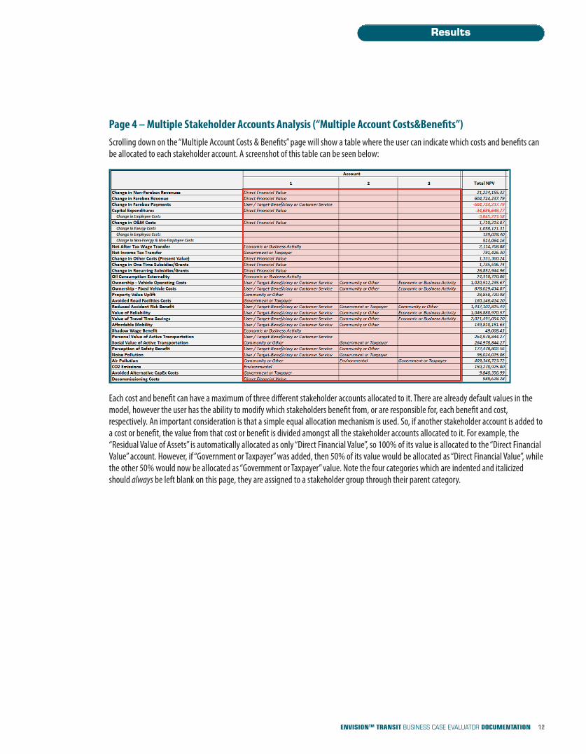
Page 4 – Multiple Stakeholder Accounts Analysis (“Multiple Account Costs&Benefits”)Scrolling down on the “Multiple Account Costs & Benefits” page will show a table where the user can indicate which costs and benefits canbe allocated to each stakeholder account. A screenshot of this table can be seen below:
Each cost and benefit can have a maximum of three different stakeholder accounts allocated to it. There are already default values in themodel, however the user has the ability to modify which stakeholders benefit from, or are responsible for, each benefit and cost, respectively. An important consideration is that a simple equal allocation mechanism is used. So, if another stakeholder account is added toa cost or benefit, the value from that cost or benefit is divided amongst all the stakeholder accounts allocated to it. For example, the “Residual Value of Assets” is automatically allocated as only “Direct Financial Value”, so 100% of its value is allocated to the “Direct FinancialValue” account. However, if “Government or Taxpayer” was added, then 50% of its value would be allocated as “Direct Financial Value”, whilethe other 50% would now be allocated as “Government or Taxpayer” value. Note the four categories which are indented and italicizedshould always be left blank on this page, they are assigned to a stakeholder group through their parent category.
Results
13ENVISIONTM TRANSIT BUSINESS CASE EVALUATOR DOCUMENTATION
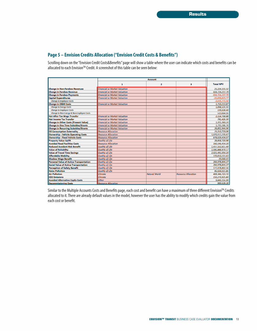
Page 5 – Envision Credits Allocation (“Envision Credit Costs & Benefits”)Scrolling down on the “Envision Credit Costs&Benefits” page will show a table where the user can indicate which costs and benefits can beallocated to each EnvisionTM Credit. A screenshot of this table can be seen below:
Similar to the Multiple Accounts Costs and Benefits page, each cost and benefit can have a maximum of three different EnvisionTM Credits allocated to it. There are already default values in the model, however the user has the ability to modify which credits gain the value fromeach cost or benefit.
Results
Benefits and Approach
DESCRIPTION OF ECONOMIC BENEFITS AND APPROACH TO VALUATION
Economic Valuation ApproachTo make a sensible comparison between different transit options, and to rank which ones should be invested in first, on needs a commonmetric. Engineering and transportation simulation methods can often quantify the differences in travel time saved and air pollution; eco-nomic methods help to put a price on these quantities so that the monetary equivalent value (price times quantity), or dollars, can be usedin the decision-making.
Engineers have at their disposal tools to calculate the effects of a transit plan on the cities, or regions, transportation network. Valuation interms of social costs (the damage or benefit to human health, buildings, crops, animals, and the environment) of the improvements is themissing link to value the benefits of sustainable projects.
Because the economics is often similar across projects, we have codified the economics and made it available to designers and engineers sothat they can understand the full economic value of their project. In this way engineers have access to tools that help them design the proj-ect right. EnvisionTM attempts to help the design process so that the project is done right from a sustainability perspective. It also helps tomake sure that the right project is done.
To compare the value and make decisions regarding the right project, one also needs to understand the risks associated with the choices.The methodology adopted combines economic cost-benefit analyses with risk analysis so that risk adjusted values are calculated, allowinginformed decision making.
Finally, infrastructure projects are complicated and affect stakeholders differently. The use of multi-account cost-benefit analysis provides abasis for understand who wins and who loses and what the basis is for cost, benefit or risk transfer. By identifying groups who, or sectorsthat, do not benefit from a project, multiple account cost-benefit analysis helps the right project, done right, get done.
“Large transport projects usually require substantial investment funding from both public and private sources. Theyoften also affect the economic and environmental characteristics of the locations where they are built. In many cases, large-scale projects affect individual stakeholder groups in idiosyncratic ways. Such stakeholder groups usually have a preferencefor voicing their views and participating in the decision-making processes preceding actual project approval, namely at the stage when alternative project alternatives or options are assessed.” [2]
BCE Links to EnvisionTM CreditsMost of the costs and benefits that are quantified in the BCE have links to credits in the EnvisionTM rating system. Some of these links arestrong (e.g. Value of Travel Time’s link to QL2.4 Improve Community Mobility and Access), and some of these links are possible but not always strong (e.g. Value of Travel Time’s link to QL2.3 Encourage Alternative Modes of Transportation). The full detailed mapping of thelinks between the BCE and credits in the EnvisionTM system, along with the associated strength of each link, can be found in Appendix A.
[2] “Multi-criteria analysis in transport project evaluation: an institutional approach” Klaas De Brucker, Cathy Macharis, and Alain Verbeke, European Transport (2011), p. 3-24
14ENVISIONTM TRANSIT BUSINESS CASE EVALUATOR DOCUMENTATION
Valuation MethodsSometimes the services transit systems provide have no price that can be directly observed as the outcome of market transactions. Economics uses several methods to value these non-market externalities. While methodologies for valuation may not vary for similar projects, often the values themselves will vary by region of the country or by income or demographics of those affected. By using meta-analyses that synthesize many studies, we hope to produce accurate results through the inclusion of geographically specific variables that include, among others, local incomes, housing values, weather patterns, and water quality.
To assign a value to things that people may never use, non-market valuation methods are employed:
n Revealed preference methods: Infer the value of a non-market good or service using other market transactions. For example, the price of a house may be used to determine the value of transit services. Hedonic pricing methods start from the premise that the price of a good is a function of the service’s characteristics. A regression model then determines the contribution of each characteristic to the market price.
n Stated preference methods: Contingent valuation studies survey people on how much they are willing to pay to get access to a goodor service or how much they would be willing to accept as compensation for a given harm or lack of access.
Market-based methods are used to measure value from the perspective of what you would have spent had you taken another approach:
n Avoided cost analysis: This methodology looks at the marginal cost of providing an equivalent service in another way. For example,increasing the number of people actively commuting to work increases the overall health of those people. One way to value this increased health is to calculate the avoided health care spending that would have been needed to obtain a similar health outcome.
Risk Analysis ApproachHigh, most likely, and low values from the literature are collected to reflect the range of uncertainty about the inputs and model assumptions. Athree-point estimation technique can then be used to construct a probability distribution representing the outcome of future events, basedon limited information. These distributions are then an input into a Monte Carlo risk analysis following a cost-benefit approach. More information is provided in Appendix B.
Social Discount RateThe social discount rate, also known as the Social Opportunity Cost of Capital, is the expected rate of return forgone from other potential investments. This rate is used to discount the stream of future costs and benefits of the project into present value terms. Therefore the valueof the social discount rate can have a large impact on the sustainable NPV of the project. For U.S. government analyses the OMB recommends using both the time preference rate (which tends to be lower and is estimated at 3% in real terms on a pre-tax basis) and theopportunity cost rate (which is higher and estimated at a real pre-tax 7% rate, reflecting the foregone rate of return). The default rate for all projects is therefore set equal to 7%. More information on the social opportunity cost of capital is provided in Appendix E.
Benefits and Approach
15ENVISIONTM TRANSIT BUSINESS CASE EVALUATOR DOCUMENTATION
Use of EnvisionTM Business Case EvaluatorThe Business Case Evaluator aims to, as much as possible:
n Be a comprehensively exhaustive list of economic benefits (where data exists). Avoiding double counting and correctly defining the scope of the project and the benefits, costs and risks to be counted is crucial to ensuring that the calculation is credible.
n To avoid error in the ultimate estimation of the total economic value associated with a given project, it will be important to avoid the potential error associated with counting a benefit associated with a given project more than once. We have tried to avoid the temptation to create a ‘grab bag’ of all possible benefits associated with these projects. We have focused attention on those benefits that are most readily monetized and where data is available. For transit, for example, hedonic house price models that attempt to capture the benefit of access to transit that is embedded in houses prices might already be accounted for in travel time savings that are also counted as a benefit. There is evidence that " the observed willingness to pay for transit station proximity most likely includes non-user benefits from proximity to transit. These non-user benefits likely amount to at least 50 percent of theobserved property value premium" Lewis-Workman, S., & Brod, D. (1997). Therefore, only 50% of the hedonic price model property uplift is counted as an incremental benefit to the travel time savings in the BCE. The non-user benefit of the property uplift is counted to the community in the stakeholder analysis and the travel time saving portion is counted as a user benefit
n There is a need to provide a clear definition of the boundary for measuring the ‘project impact’ in order to consistently measure benefit/credits across categories. For instance, is the boundary of impact spatial or non-spatial? A clear understanding/method for estimating the project boundary will be needed. This will directly impact the inclusion/exclusion of project benefits/credits.
n Measure the risk associated with the business case costs and benefits.
n There are often many ways to measure the same benefit. Often, meta-analyses of benefits use studies that mix several techniques.In theory, willingness to pay (WTP) and willingness to accept (WTA) should give the same results but in experiments they have shown that measures of WTA greatly exceed measures of WTP. As meta-analyses have done, we average results over several methodologies (but also capturing the range that is produced from these methodologies too). For a particular benefit, one methodology for measurement and monetization may dominate and in another a range of methodologies may be used. The objective is to use the state of the art in measurement of these externalities. In this regard transparency trumps consistency of one particular method.
n Be a reference document that documents the sustainable return of the infrastructure project. The analysis is done relative to a reference case, which is equivalent to the status quo or a “do nothing” scenario. Often, refurbishment or increased operations and maintenance costs of an existing facility are required if a project does not go ahead. These expenditures should be included in the reference case. The Business Case Evaluator also has the capacity for individual projects to be compared against each other, so that if a “do nothing” scenario is not a viable option, then results valuing different project options against each other may be obtained.
Each cost or benefit that is quantified in the business case evaluator has been included because it:
n Is significant on a list of costs and benefits that aims to be comprehensively exhaustive when describing the impacts of transit projects,
n Has substantial literature surrounding its quantification so that reliable and consistent values can be obtained, even as the model is applied across different geographical regions.
Because of the risk and cost benefit framework, the use of the business case evaluator may fulfill some requirements for EnvisionTM credits.
Benefits and Approach
16ENVISIONTM TRANSIT BUSINESS CASE EVALUATOR DOCUMENTATION
Descriptions & Definitions
17ENVISIONTM TRANSIT BUSINESS CASE EVALUATOR DOCUMENTATION
yp p
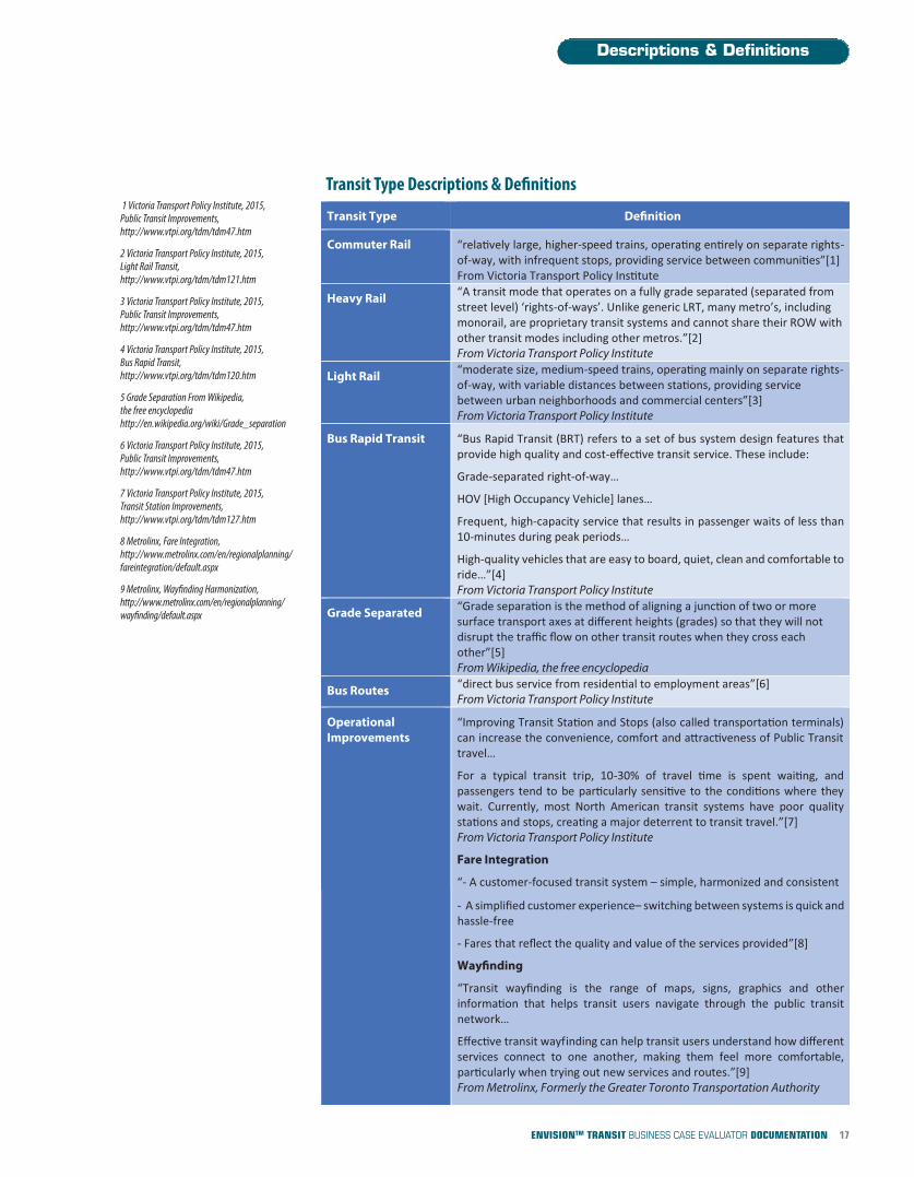
Transit Type DeÞnition
Commuter Rail “rela vely large, higher-speed trains, opera ng en rely on separate rights-of-way, with infrequent stops, providing service between communi es”[1] From Victoria Transport Policy Ins tute
Heavy Rail “A transit mode that operates on a fully grade separated (separated from street level) ‘rights-of-ways’. Unlike generic LRT, many metro’s, including monorail, are proprietary transit systems and cannot share their ROW with other transit modes including other metros.”[2] From Victoria Transport Policy Institute
Light Rail “moderate size, medium-speed trains, opera ng mainly on separate rights-of-way, with variable distances between sta ons, providing service between urban neighborhoods and commercial centers”[3] From Victoria Transport Policy Institute
Bus Rapid Transit “Bus Rapid Transit (BRT) refers to a set of bus system design features that provide high quality and cost-effec ve transit service. These include:
Grade-separated right-of-way…
HOV [High Occupancy Vehicle] lanes…
Frequent, high-capacity service that results in passenger waits of less than 10-minutes during peak periods…
High-quality vehicles that are easy to board, quiet, clean and comfortable to ride…”[4] From Victoria Transport Policy Institute
Grade Separated “Grade separa on is the method of aligning a junc on of two or more surface transport axes at different heights (grades) so that they will not disrupt the traffic flow on other transit routes when they cross each other”[5] From Wikipedia, the free encyclopedia
Bus Routes “direct bus service from residen al to employment areas”[6] From Victoria Transport Policy Institute
Operational Improvements
“Improving Transit Sta on and Stops (also called transporta on terminals) can increase the convenience, comfort and a#rac veness of Public Transit travel…
For a typical transit trip, 10-30% of travel me is spent wai ng, and passengers tend to be par cularly sensi ve to the condi ons where they wait. Currently, most North American transit systems have poor quality sta ons and stops, crea ng a major deterrent to transit travel.”[7] From Victoria Transport Policy Institute
Fare Integration
“- A customer-focused transit system – simple, harmonized and consistent
- A simplified customer experience– switching between systems is quick and hassle-free
- Fares that reflect the quality and value of the services provided”[8]
WayÞnding
“Transit wayfinding is the range of maps, signs, graphics and other informa on that helps transit users navigate through the public transit network…
Effec ve transit wayfinding can help transit users understand how different services connect to one another, making them feel more comfortable, par cularly when trying out new services and routes.”[9] From Metrolinx, Formerly the Greater Toronto Transportation Authority
Transit Type Descriptions & Definitions1 Victoria Transport Policy Institute, 2015,
Public Transit Improvements,http://www.vtpi.org/tdm/tdm47.htm
2 Victoria Transport Policy Institute, 2015, Light Rail Transit,http://www.vtpi.org/tdm/tdm121.htm
3 Victoria Transport Policy Institute, 2015, Public Transit Improvements,http://www.vtpi.org/tdm/tdm47.htm
4 Victoria Transport Policy Institute, 2015, Bus Rapid Transit,http://www.vtpi.org/tdm/tdm120.htm
5 Grade Separation From Wikipedia, the free encyclopediahttp://en.wikipedia.org/wiki/Grade_separation
6 Victoria Transport Policy Institute, 2015, Public Transit Improvements,http://www.vtpi.org/tdm/tdm47.htm
7 Victoria Transport Policy Institute, 2015, Transit Station Improvements,http://www.vtpi.org/tdm/tdm127.htm
8 Metrolinx, Fare Integration,http://www.metrolinx.com/en/regionalplanning/fareintegration/default.aspx
9 Metrolinx, Wayfinding Harmonization,http://www.metrolinx.com/en/regionalplanning/wayfinding/default.aspx
Economic Benefits
“Customized application of nonmarket valuation methods can be expensive and time consuming to perform. Contingent valuation, for example, can require conducting survey research; a hedonic pricing study may involve extensive data assembly.” [3]
While expensive, the preferred approach will always be for the use of directly measured benefits. To the extent that project, local, or re-gional data, are available and is consistent with the measurement of the benefit category, it should be used. An example may be that a sur-vey is available of local residents that measures WTP for saving a minute of commuting time. Where information is not available the“benefits transfer” approach is used. This takes benefits calculated for other projects, perhaps in other areas or for different types of projectsand uses the estimates for the current infrastructure project adjusted for local conditions and design. In design of the tool then we haveadopted the philosophy that the user should always have the option of entering data to override defaults with more appropriate data.
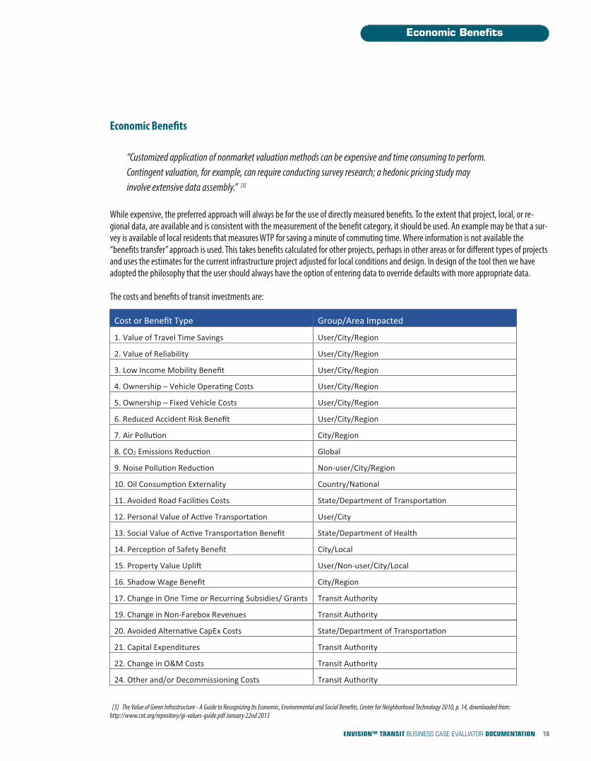
The costs and benefits of transit investments are:
Economic Benefits
[3] The Value of Green Infrastructure - A Guide to Recognizing Its Economic, Environmental and Social Benefits, Center for Neighborhood Technology 2010, p. 14, downloaded from:http://www.cnt.org/repository/gi-values-guide.pdf January 22nd 2013
Cost or Benefit Type Group/Area Impacted
1. Value of Travel Time Savings User/City/Region
2. Value of Reliability User/City/Region
3. Low Income Mobility Benefit User/City/Region
4. Ownership – Vehicle Opera ng Costs User/City/Region
5. Ownership – Fixed Vehicle Costs User/City/Region
6. Reduced Accident Risk Benefit User/City/Region
7. Air Pollu on City/Region
8. CO2 Emissions Reduc on Global
9. Noise Pollu on Reduc on Non-user/City/Region
10. Oil Consump on Externality Country/Na onal
11. Avoided Road Facili es Costs State/Department of Transporta on
12. Personal Value of Ac ve Transporta on User/City
13. Social Value of Ac ve Transporta on Benefit State/Department of Health
14. Percep on of Safety Benefit City/Local
15. Property Value Upli! User/Non-user/City/Local
16. Shadow Wage Benefit City/Region
17. Change in One Time or Recurring Subsidies/ Grants Transit Authority
19. Change in Non-Farebox Revenues Transit Authority
20. Avoided Alterna ve CapEx Costs State/Department of Transporta on
21. Capital Expenditures Transit Authority
22. Change in O&M Costs Transit Authority
24. Other and/or Decommissioning Costs Transit Authority
18ENVISIONTM TRANSIT BUSINESS CASE EVALUATOR DOCUMENTATION
Increased Revenues and Avoided CostsThe first costs and benefits that are incorporated into the model’s calculations are the direct financial costs and benefits, including capital expen-ditures, operations and maintenance costs, non-fare-box revenues, other costs, and a change in subsidies obtained. The impacts of a project onemployee and energy costs are inferred based on capital expenditures and O&M costs. These are not counted in the final value of the analysis asthey are fully captured in capital expenditures and O&M costs. They are only included for accounting purposes when allocating values to variousstakeholder groups in the Multi-Account Evaluation (MAE). The remaining costs, and subsidies, are all calculated using values that are input bythe user that indicate what those costs would be in a status quo scenario, as well as what those values are expected to be after the proposedproject is in operation.
Furthermore fare-box revenues are calculated directly in the model based on the projected ridership and trip fares. These revenues are not an in-cremental benefit as they are simply a transfer of wealth between transit riders and the transit authority. Therefore, in the sustainable analysisthe offsetting transfer, the change in fare-box payments, is included to account for this. In other words, these are both treated as transfers andare only included in the analysis for the Multi-Account Evaluation (MAE).
Components:
n Project capital costsn Project O&M costs in the base case and transit casen Changes in subsidies received n Employee & energy costsn Changes in faresn Changes in ridershipn Changes in non-fare-box revenue
Includes: The financial costs and benefits of the project
Excludes: Social values and/or externalities
Default Stakeholder Groups:
Capital Expenditures, O&M Costs, Fare-box Revenue, & Non-fare-box Revenue → 100% Direct Financial Value
Change in Fare-box Payments → 100% User/Target-Beneficiary or Customer Service
Default Envision Categories: 100% Financial or Market Valuation
Revenues & Avoided Costs
19ENVISIONTM TRANSIT BUSINESS CASE EVALUATOR DOCUMENTATION
Value of Travel Time Savings
This benefit category has two components: the value of travel time savings and the value of congestion. The value of both of these components are added together to obtain the total value of travel time savings reported in the BCE. The theoretical underpinning and empirical estimation strategy for both components is explained below.
The Value of Travel Time SavingsThe value of time (VOT) savings, also referred to as the value of travel time savings (VTTS), is defined as the willingness to pay for a unit (minute) oftravel time savings.[4] On average this accounts for the largest portion of monetized benefits in the evaluation of road and transit projects account-ing for approximately 80% of the monetized benefits in the UK[5] and, from our experience, this is also the case in North America.
Due to the large share of the benefits which amass from the VOT, it is useful to understand the microeconomic theory behind its calculation.The value of time used in transportation is based on research that values time in different activities differently: leisure, getting to work by different transportation modes, waiting, and travelling and waiting in different levels of comfort and certainty.
The concept of the VOT is linked to the study of labor demand and supply. The VOT originates from the idea that time is a finite resource tobe split among either working or leisure. Thus the VOT was originally thought to be equal to the opportunity cost of an additional unit ofleisure time, which is equal to the forgone wage.[6]
The concept of the VOT was expanded with Becker’s theory of time as an input in the production of household goods. This theory postulatedthat households don’t consume goods directly, but rather consume ‘final goods’ which are the combination of market goods and time.[7]
This theory had two implications in the field of transportation research. First, consumers were not only constrained by income but also bytime. Since time can be converted to income via work the opportunity cost of time is, again, equal to the wage rate. Second, this theory recognizes that the demand for travel is actually derived from the demand for goods which requires out-of-home travel. Consumers werenow thought to have to consider consumption that requires travel, and that travel requires time.[8]
DeSerpa expanded and refined the theory further by recognizing that some activities are assigned more time than consumers want to because of some type of constraint. This is the model where contemporary estimations of the VTTS come from. DeSerpa postulated thatthere may be activities that individuals would like to shorten but cannot; this implies that they cannot be adjusted to be equal to the valueof foregone work. This creates a new element in the economic theory of time: “the reassignment of time from one activity to another can bepleasurable not only because one does more of the latter, but also because one does less of the former.” [9] This theory led to three types ofvalues of time: the value of time as a resource, the value of time as a commodity, and the value of saving time on an activity.
The value of time as a resource is defined as the resource value of extending the time period, which is equivalent to the ratio of marginalutility of time to the marginal utility of income. The value of time as a commodity is the value of time allocated to a certain activity. Thisequates to the individuals rate of substitution between that specific activity and money in their individual utility function. Finally the valueof saving time on a specific activity is the difference between the resource value of time and the value of time as a commodity for that specific activity.
Travel Time Savings
20ENVISIONTM TRANSIT BUSINESS CASE EVALUATOR DOCUMENTATION
[4] “Synthesis of Research on Value of Time and Value of Reliability”, 2009, Sisinnio Concas et al., Florida Department of Transportation.[5] “The value of travel time savings in evaluation”, 2001, P.J. Mackie et al., Transportation Research Part E.[6] Sisinnio Concas, op. cit.[7] “A theory of the allocation of time”, 1965, Gary Becker, The Economic Journal 75, 493-517.[8] Mackie et al., op. cit.[9] Mackie et al., op. cit.
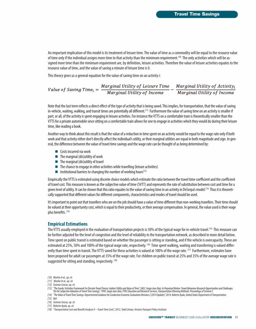
An important implication of this model is its treatment of leisure time. The value of time as a commodity will be equal to the resource valueof time only if the individual assigns more time to that activity than the minimum requirement.[10] The only activities which will be as-signed more time than the minimum requirement are, by definition, leisure activities. Therefore the value of leisure activities equates to theresource value of time, and the value of saving a minute of leisure time is 0.
This theory gives us a general equation for the value of saving time on an activity i:
Note that the last term reflects a direct effect of the type of activity that is being saved. This implies, for transportation, that the value of savingin-vehicle, waiting, walking, and transit times are potentially all different.[11] Furthermore the value of saving time on an activity is smaller ifpart, or all, of the activity is spent engaging in leisure activities. For instance the VTTS on a comfortable train is theoretically smaller than theVTTS for a private automobile since sitting on a comfortable train allows for one to engage in activities which they would do during their leisuretime, like reading a book.
Another way to think about this result is that the value of a reduction in time spent on an activity would be equal to the wage rate only if bothwork and that activity either don’t directly affect the individual’s utility, or their marginal utilities are equal in both magnitude and sign. In gen-eral, the difference between the value of travel time savings and the wage rate can be thought of as being determined by:
n Costs incurred via workn The marginal (dis)utility of workn The marginal (dis)utility of traveln The chance to engage in other activities while travelling (leisure activities)n Institutional barriers to changing the number of working hours[12]
Empirically the VTTS is estimated using discrete choice models which estimate the ratio between the travel time coefficient and the coefficientof travel cost. This measure is known as the subjective value of time (SVTT) and represents the rate of substitution between cost and time for agiven level of utility. It can be shown that this ratio equates to the value of saving time in an activity in DeSerpa’s model.[13] Thus it is theoreti-cally supported that different values for different components, characteristics and modes of travel should be used.
It’s important to point out that travellers who are on the job should have a value of time different than non-working travellers. Their time shouldbe valued at their opportunity cost, which is equal to their productivity, or their average compensation. In general, the value used is their wageplus benefits. [14]
Empirical EstimationsThe VTTS usually employed in the evaluation of transportation projects is 50% of the typical wage for in-vehicle travel.[15] This measure canbe further adjusted for the level of congestion and the level of reliability in the transportation network, as described in more detail below.Time spent on public transit is estimated based on whether the passenger is sitting or standing, and if the vehicle is overcapacity. These areestimated at 25%, 50% and 100% of the typical wage rate, respectively. [16] Time spent walking, waiting and transferring is valued differ-ently than time spent in transit. The VTTS saved for these activities is valued at 100% of the wage rate. [17] Furthermore, estimates havebeen proposed for adult car passengers at 35% of the wage rate. For children on public transit at 25% and 35% of the average wage rate issuggested for sitting and standing, respectively. [18]
Travel Time Savings
21ENVISIONTM TRANSIT BUSINESS CASE EVALUATOR DOCUMENTATION
[10] Mackie et al., op. cit.[11] Mackie et al., op. cit.[12] Sisinnio Concas, op. cit.[13] “The Goods/ Activities Framework For Discrete Travel Choices: Indirect Utility and Value of Time”, 2002, Sergio Jara-Diaz, In Perpetual Motion: Travel Behaviour Research Opportunities and Challenges.
“On the Subjective Valuation of Travel Time Savings”, 1999, Sergio Jara-Diaz, PTRC Education and Research Services, Transportation Planning Methods: Proceedings of Seminar F.[14] “The Value of Travel Time Savings: Departmental Guidance for Conduction Economic Evaluations Revision 2 (2014 Update)”, 2014, Roberto Ayala, United States Department of Transportation.[15] Ibid[16] Sisinnio Concas, op. cit.[17] Roberto Ayala, op. cit.[18] “Transportation Cost and Benefit Analysis II – Travel Time Costs”, 2012, Todd Litman, Victoria Transport Policy Institute.
Work and Non-Work TravelAn important factor when calculating VTTS is knowing the mix of work and non-work travel taking place on the transportation system. ForU.S. roads the U.S. DOT provides recommended values. The recommended mix for local inner city roads is 5% work and 95% non-work, andfor intercity roads the recommended mix is 21% work and 79% non-work travel. [19]
Vehicle Occupancy RateIt is also important to know the vehicle occupancy rate when calculating the VTTS as assuming one person per vehicle would be erroneous.For the U.S., these values are provided in the U.S. DOT’s National Household Travel Survey. Vehicle occupancy is broken down by the follow-ing trip purposes: commuting, shopping, personal errands, and social and recreation. Across all purposes the average vehicle occupancy is1.67 passengers per car. However for commuting to and from work vehicle occupancy is much lower at 1.13 passengers per car. This implies different vehicle occupancy rates at different times of the day and week should be applied when calculating VTTS.
WagesSince VTTS is calculated as a portion of the prevailing wage rate a key question for estimating the VTTS is which wage rate to use.
Mean vs. Median Wages
The U.S. DOT suggests the use of the median wage rate. [20] This is logical as the income distribution is highly skewed, implying that the medianwage is more representative of the general population than the mean.
National vs. Local Wages
Since the value of time saved for an activity depends on each individual's marginal utility, the wage rate should theoretically be based oneach individual's wage rate. This implies that the wage rate should be adjusted to represent, as best as possible, the group of users usingthe transportation system. Thus the regional, or metro-area, wage rate is the preferred wage rate.
Travel Time Savings
22ENVISIONTM TRANSIT BUSINESS CASE EVALUATOR DOCUMENTATION
[19] Roberto Ayala, op. cit.[20] Roberto Ayala, op. cit.
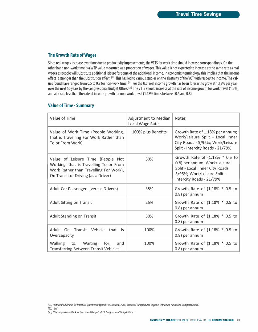
The Growth Rate of WagesSince real wages increase over time due to productivity improvements, the VTTS for work time should increase correspondingly. On theother hand non-work time is a WTP value measured as a proportion of wages. This value is not expected to increase at the same rate as realwages as people will substitute additional leisure for some of the additional income. In economics terminology this implies that the incomeeffect is stronger than the substitution effect. [21] This has led to various studies on the elasticity of the VOT with respect to income. The val-ues found have ranged from 0.5 to 0.8 for non-work time. [22] For the U.S. real income growth has been forecast to grow at 1.18% per yearover the next 50 years by the Congressional Budget Office. [23] The VTTS should increase at the rate of income growth for work travel (1.2%),and at a rate less than the rate of income growth for non-work travel (1.18% times between 0.5 and 0.8).
Value of Time - Summary
Travel Time Savings
23ENVISIONTM TRANSIT BUSINESS CASE EVALUATOR DOCUMENTATION
Value of Time Adjustment to Median Local Wage Rate
Notes
Value of Work Time (People Working, that is Travelling For Work Rather than To or From Work)
100% plus Benefits Growth Rate of 1.18% per annum; Work/Leisure Split - Local Inner City Roads - 5/95%; Work/Leisure Split - Intercity Roads - 21/79%
Value of Leisure Time (People Not Working, that is Travelling To or From Work Rather than Travelling For Work), On Transit or Driving (as a Driver)
50%
Adult Car Passengers (versus Drivers) 35% Growth Rate of (1.18% * 0.5 to 0.8) per annum
Adult Si ng on Transit 25% Growth Rate of (1.18% * 0.5 to 0.8) per annum
Adult Standing on Transit 50% Growth Rate of (1.18% * 0.5 to 0.8) per annum
Adult On Transit Vehicle that is Overcapacity
100% Growth Rate of (1.18% * 0.5 to 0.8) per annum
Walking to, Wai!ng for, and Transferring Between Transit Vehicles
100% Growth Rate of (1.18% * 0.5 to 0.8) per annum
Growth Rate of (1.18% * 0.5 to 0.8) per annum; Work/Leisure Split - Local Inner City Roads 5/95%; Work/Leisure Split - Intercity Roads - 21/79%
[21] “National Guidelines for Transport System Management in Australia”, 2006, Bureau of Transport and Regional Economics, Australian Transport Council.[22] Ibid[23] “The Long-Term Outlook for the Federal Budget”, 2013, Congressional Budget Office.
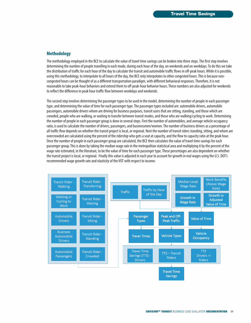
MethodologyThe methodology employed in the BCE to calculate the value of travel time savings can be broken into three steps. The first step involves determining the number of people travelling in each mode, during each hour of the day, on weekends and on weekdays. To do this we takethe distribution of traffic for each hour of the day to calculate the transit and automobile traffic flows in off-peak hours. While it is possible,using this methodology, to interpolate to all hours of the day, the BCE only interpolates to other congested hours. This is because non-congested hours can be thought of as a different transportation paradigm, with different behavioral responses. Therefore, it is not reasonable to take peak-hour behaviors and extend them to off-peak-hour behavior hours. These numbers are also adjusted for weekendsto reflect the difference in peak hour traffic flow between weekdays and weekends.
The second step involves determining the passenger types to be used in the model, determining the number of people in each passengertype, and determining the value of time for each passenger type. The passenger types included are: automobile drivers, automobile passengers, automobile drivers whom are driving for business purposes, transit users that are sitting, standing, and those which arecrowded, people who are walking, or waiting to transfer between transit modes, and those who are walking/cycling to work. Determiningthe number of people in each passenger group is done in several steps. First the number of automobiles, and average vehicle occupancyratio, is used to calculate the number of drivers, passengers, and businessmen/women. The number of business drivers as a percentage ofall traffic flow depends on whether the transit project is local, or regional. Next the number of transit riders standing, sitting, and whom areovercrowded are calculated using the percent of the ridership who gets a seat at capacity, and the flow to capacity ratio at the peak hour.Once the number of people in each passenger group are calculated, the BCE then calculates the value of travel time savings for each passenger group. This is done by taking the median wage rate in the metropolitan statistical area and multiplying it by the percent of thewage rate estimated, in the literature, to be the value of time for each passenger type. These percentages are also dependent on whetherthe transit project is local, or regional. Finally this value is adjusted in each year to account for growth in real wages using the U.S. DOT’s recommended wage growth rate and elasticity of the VOT with respect to income.
Travel Time Savings
24ENVISIONTM TRANSIT BUSINESS CASE EVALUATOR DOCUMENTATION
In the final step the BCE calculates the travel time savings for each passenger group and applies the above value of time to obtain the value oftravel time savings. This is done for three categories of people in the transportation network: those who were automobile drivers in the base caseand remain drivers, those who were used transit in the base case and remain transit users, and those who switch from driving to taking transit. Thevalue of travel time savings of all three categories of people are then summed to obtain the final value of travel time savings.
Components: n Local wage rates, and the growth rate of real wagesn Forecasts of traffic and transit flowsn Distribution of traffic flow by hourn Ratio of weekend peak traffic flow to weekday peak traffic flown Transit opening and closing hoursn Average, and changes in, the vehicle occupancy ratio
Includes: The social value of saving travel time and changes in travel conditions
Excludes: Evaluation of equity implications for different socioeconomic groups
Default Stakeholder Group: 33% User/Target Beneficiary, 33% Community, 33% Economic or Business Activity
Default Envision Categories: 100% Quality of Life
Travel Time Savings
25ENVISIONTM TRANSIT BUSINESS CASE EVALUATOR DOCUMENTATION
The Value of Congestion It is a well-studied fact that “the value motorists place upon travel time…can be expected to vary with traffic conditions.” [24] This reflectsthe fact that driving in congestion is more difficult due to the higher number of vehicles on the road. Additionally individuals are likely tohave a greater disutility for driving in congestion as it is more stressful, frustrating and perhaps also due to a heightened feeling of danger. [25] Putanother way, driving in congested traffic, is a different activity than driving in uncongested traffic that is further away from what can bethought of as leisure. Therefore saving time spent driving in congested traffic warrants a higher value than non-congested traffic. This hasled to the study of the ‘congestion multiplier’. The value of this multiplier scales the VOT during congested periods and hence the VTTS fromrelieving congestion during rush hours.
A meta-analysis of 38 studies covering 100 congestion multipliers reveals their value to be between 1.3 and 2.0, which clearly indicatesthat saving time spent in congested traffic is has a higher value than saving time in free-flow conditions. The meta-analysis investigatedand provided clear evidence that the multiplier increases as driving conditions become more difficult. Furthermore congestion was notfound to be different when it was valued on urban or interurban roads. There was also no difference when the value of the congestion wasderived from a study on tolled infrastructure. [26] Another meta-analysis of UK values of travel time savings found an average multiplier of1.54, with a standard deviation of 0.33 across 9 studies which covered 29 valuations of the congestion multiplier. [27]
There is the view that congestion multipliers contain an element of unreliability, and some practitioners advocate the inclusion of somekind of reliability variable alongside car time variables. However, a recent meta-analysis of congestion multipliers show that including a reliability variable does not, in a statistically significant way, change the estimated congestion multiplier. [28]
Possibly the most important finding in the congestion literature is that the congestion multiplier increases as road conditions worsen andtraffic density increases. Therefore it is helpful to have a definition for different levels of congestion:
n Free flowing: you can travel at your own speed with no problems over-taking;
n Busy: you can travel pretty much at the speed limit, but you are forced to change lanes every now and then;
n Light congestion: you can travel close to the speed limit most of the time, but you have to slow down every so often for no apparent reason;
n Heavy congestion: your speed is noticeably restricted with frequent gear changes required;
n Stop-start: you are forced to drive in a ‘stop-start’ fashion;
n Gridlock: you are only able to move at a crawl at best, and spend quite a lot of time stationary. [29]
Value of Congestion
26ENVISIONTM TRANSIT BUSINESS CASE EVALUATOR DOCUMENTATION
[24] “The congestion multiplier: Variations in motorists’ valuation of travel time with traffic conditions”, 2012, Mark Wardman and J. Nicolas Ibanez, Transportation Research Part A.[25] Ibid[26] Ibid[27] “Meta-Analysis of UK Values of Time: An Update”, 2009, Pedro Abrantes and Mark Wardman, Institute for Transport Studies, Transportation Research Part A.[28] Mark Wardman and J. Nicolas Ibanez, op. cit.[29] “Effect of Road Congestion on Rail Demand: Technical Report“, 2004, Steer Davies Gleave, Prepared for Passenger Demand Forecasting Council, Association of Train Operating Companies, London.
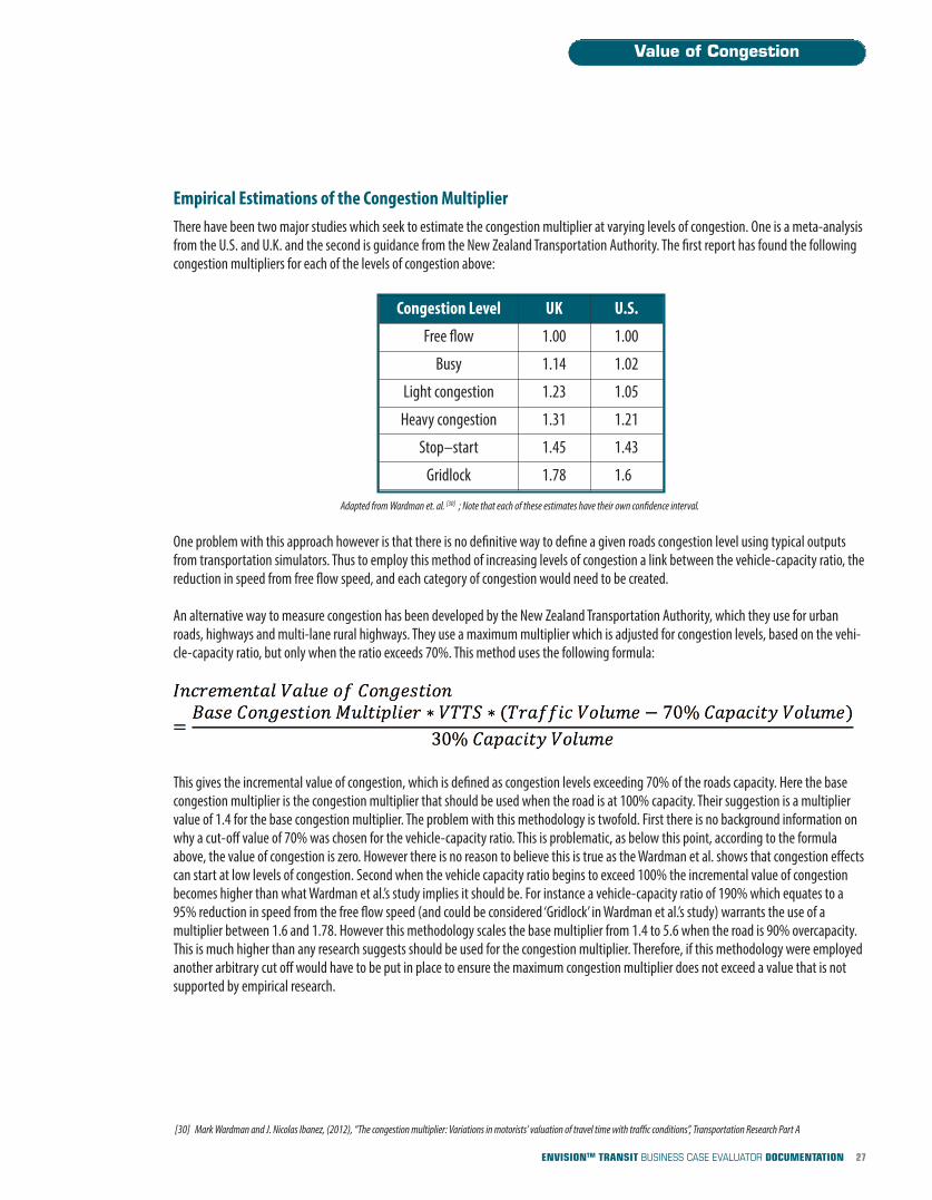
Value of Congestion
Empirical Estimations of the Congestion MultiplierThere have been two major studies which seek to estimate the congestion multiplier at varying levels of congestion. One is a meta-analysisfrom the U.S. and U.K. and the second is guidance from the New Zealand Transportation Authority. The first report has found the followingcongestion multipliers for each of the levels of congestion above:
Adapted from Wardman et. al. [30] ; Note that each of these estimates have their own confidence interval.
One problem with this approach however is that there is no definitive way to define a given roads congestion level using typical outputsfrom transportation simulators. Thus to employ this method of increasing levels of congestion a link between the vehicle-capacity ratio, thereduction in speed from free flow speed, and each category of congestion would need to be created.
An alternative way to measure congestion has been developed by the New Zealand Transportation Authority, which they use for urbanroads, highways and multi-lane rural highways. They use a maximum multiplier which is adjusted for congestion levels, based on the vehi-cle-capacity ratio, but only when the ratio exceeds 70%. This method uses the following formula:
This gives the incremental value of congestion, which is defined as congestion levels exceeding 70% of the roads capacity. Here the basecongestion multiplier is the congestion multiplier that should be used when the road is at 100% capacity. Their suggestion is a multipliervalue of 1.4 for the base congestion multiplier. The problem with this methodology is twofold. First there is no background information onwhy a cut-off value of 70% was chosen for the vehicle-capacity ratio. This is problematic, as below this point, according to the formulaabove, the value of congestion is zero. However there is no reason to believe this is true as the Wardman et al. shows that congestion effectscan start at low levels of congestion. Second when the vehicle capacity ratio begins to exceed 100% the incremental value of congestionbecomes higher than what Wardman et al.’s study implies it should be. For instance a vehicle-capacity ratio of 190% which equates to a95% reduction in speed from the free flow speed (and could be considered ‘Gridlock’ in Wardman et al.’s study) warrants the use of a multiplier between 1.6 and 1.78. However this methodology scales the base multiplier from 1.4 to 5.6 when the road is 90% overcapacity.This is much higher than any research suggests should be used for the congestion multiplier. Therefore, if this methodology were employedanother arbitrary cut off would have to be put in place to ensure the maximum congestion multiplier does not exceed a value that is notsupported by empirical research.
[30] Mark Wardman and J. Nicolas Ibanez, (2012), “The congestion multiplier: Variations in motorists’ valuation of travel time with traffic conditions”, Transportation Research Part A
27ENVISIONTM TRANSIT BUSINESS CASE EVALUATOR DOCUMENTATION
Congestion Level UK U.S.
Free flow 1.00 1.00
Busy 1.14 1.02
Light congestion 1.23 1.05
Heavy congestion 1.31 1.21
Stop–start 1.45 1.43
Gridlock 1.78 1.60
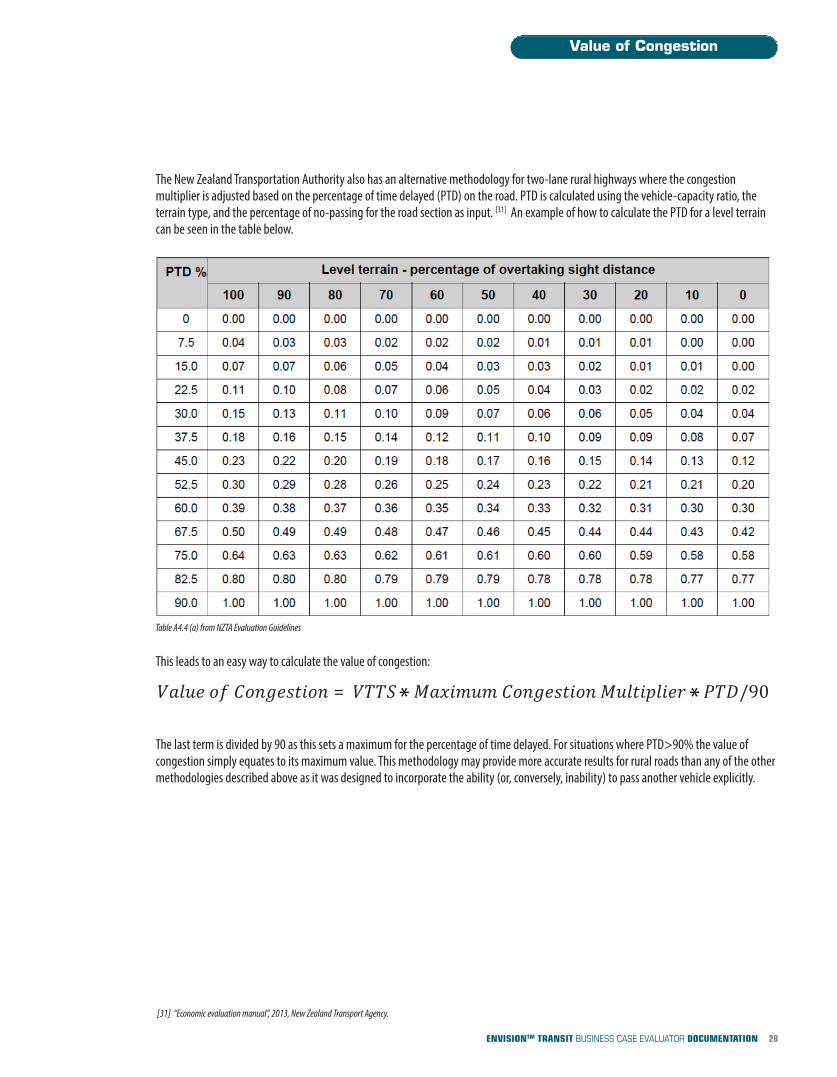
Value of Congestion
The New Zealand Transportation Authority also has an alternative methodology for two-lane rural highways where the congestion multiplier is adjusted based on the percentage of time delayed (PTD) on the road. PTD is calculated using the vehicle-capacity ratio, the terrain type, and the percentage of no-passing for the road section as input. [31] An example of how to calculate the PTD for a level terrain can be seen in the table below.
This leads to an easy way to calculate the value of congestion:
The last term is divided by 90 as this sets a maximum for the percentage of time delayed. For situations where PTD>90% the value of congestion simply equates to its maximum value. This methodology may provide more accurate results for rural roads than any of the othermethodologies described above as it was designed to incorporate the ability (or, conversely, inability) to pass another vehicle explicitly.
28ENVISIONTM TRANSIT BUSINESS CASE EVALUATOR DOCUMENTATION
= /90 * *
Table A4.4 (a) from NZTA Evaluation Guidelines
[31] “Economic evaluation manual”, 2013, New Zealand Transport Agency.
Because of the problems with the New Zealand study giving results beyond those reported by Wardman et. al. (2012) we use the more conservative results from the latter study in the BCE.
Methodology
As the value of congestion is an adjustment to the value of travel time savings it is not broken out as its own category, but rather it is included in the value of travel time savings reported in the model. To adjust the value of travel time savings for congestion we first need tocreate a link between the congestion levels, listed above from Wardman et. al. (2012), and the decrease in speed necessary to achieve eachspecific level of congestion. This was done by matching the definitions of each of the congestion levels to a percent decrease in speed. Next the congestion multiplier for the prevailing level of congestion is calculated. If the level of congestion is exactly equal to one of thedefinitions, the range of values for that level of congestion is used. On the other hand, if the level of congestion is between two definitionsa linear trend between those two points is used to infer the relevant congestion multiplier. The congestion multiplier is then used to adjustthe value of travel time savings, for commuters and business drivers, as calculated above. This increases the value of travel time savings in highly congested periods.
Components:
n Level of congestion for the projected forecast of traffic flow
n The value of time, by passenger type
Includes: The value of stressful driving situations
Excludes: The value of variations in travel times
Default Stakeholder Group: 33% User/Target Beneficiary, 33% Community, 33% Economic or Business Activity
Default Envision Categories: 100% Quality of Life
Value of Congestion
29ENVISIONTM TRANSIT BUSINESS CASE EVALUATOR DOCUMENTATION
Value of Reliability“Trip time reliability is measured by the unpredictable variations in journey times, which are experienced for a journey undertaken atbroadly the same time every day. This is distinct from the variations in individual journey times, which occur within a particular period.” [32]
Reliability is a concept separate from congestion: “Reliability draws on the attribute of predictability… a congested road system where thespeeds at different times of the day and different days of the week are consistent and hence, predictable, would be ranked as highly reliable.” [33] Another way to think of reliability is as travel time variability. Travel times are inherently variable and time variability is costly.Many professionals believe as a result that the reliability of transportation systems is grossly undervalued in project evaluation. When a system is unreliable individuals may add a buffer time to allow for the possibility of delay and companies will adapt their business practicesand timing of their operations. [34] The value business travellers and commuters place on a reliable transportation network is known as theValue of Reliability (VOR).
A recent summit hosted by the OECD and the International Transport Forum has provided the means for coherently adding reliability intocost-benefit assessments to encourage the proper evaluation of options which deliver differing levels of reliability. This summit summarizedthe ways to measure and value reliability and how this has been used in various countries already.
Measuring ReliabilityThere are several metrics that can be used to measure travel time variability, each with their own advantages and disadvantages:
n The standard deviation of travel times. This is easy to measure and estimate but it assumes a symmetric distribution of travel times.
n A buffer time index, measured as the difference between the travel time at the 80th, 90th, or 95th percentile of travel times and the 50th. This measure equates the number of minutes a commuter needs to add to their trip to only be late 20%, 10% or 5% percent the time, respectively. This measure relaxes the assumption of a symmetric distribution but requires more data.
n Risk measures such as the probability of a delay of a certain length can also be used. These measures don’t assume a symmetric distribution but also require more data.
n Scheduling measures can be used which estimate the optimal departure time to minimize the aggregate cost of being late or early. This is the theoretically correct way to measure reliability but requires detailed origin-destination information about each commuter.
[32] “Economic evaluation manual” 2013, New Zealand Transport Agency.[33] “Improving Reliability on Surface Transport Networks”, 2010, Transport Research Centre, International Transport Forum, OECD.[34] Ibid
Value of Reliability
30ENVISIONTM TRANSIT BUSINESS CASE EVALUATOR DOCUMENTATION
Theoretical Models of VORTwo approaches have been applied to arrive at values for reliability: the scheduling model, and the mean-variance approach.
The scheduling model characterizes commuter behavior by estimating the demand function for reliability. This can be thought of as the behavioral approach. In these models unreliability is measured as the number of minutes that an individual will depart or arrive earlier, orlater, than they prefer. [35] This method distinguishes between the costs of being early and late, which are not assumed to be the same. Inthe scheduling model, variability costs are captured indirectly through modelling traveller’s optimal departure time choices. Since theyknow there will be variability, they adjust their departure time to adjust the probability of being late, or early. [36] The monetary values ob-tained from this approach are hard to implement in a cost-benefit analysis due to the lack of information about desired time of arrivals.
The mean-variance approach, on the other hand, uses the standard deviation (or variance) of the travel time distribution. This can bethought of as the analytical approach. This approach specifies a reduced-form utility function which includes the mean journey duration aswell as the standard deviation of the journey:
α =β Time+ γ Cost+ δ Standard Deviation of Travel TimeVTTS= β ⁄ γVOR= δ ⁄ γ
Reliability Ratio (RR)≡ ρ= δ ⁄ β =VOR/VTTSThis approach is relatively straightforward to apply in project evaluation, as it simply requires scaling the VTTS by the reliability ratio (RR)but it lacks a strong theoretical underpinning. However it has been shown that this approach can be derived from the scheduling model aslong as the shape of the travel time distribution remains unchanged. [37] Furthermore this approach relies on the standard deviation oftravel times, which assumes that the travel time distribution is symmetric. Yet many researchers believe the distribution is skewed to theright, implying that longer than usual travel times are more common than shorter than usual travel times. However recent empirical stud-ies suggest that on many transportation links the distribution exhibits no statistically significant skew, and it is only on a small amount oflinks that a right skew is detected. [38]
Reliability can also be applied to public transit by using a measure of the average lateness around the scheduled arrival time. This measureof reliability may be harder to obtain and is thus subject to greater data requirements.
Empirical Estimations of the Value of Reliability (VOR)The estimation of VOR is straight forward and is usually calculated as:
VOR = RR * σ * VVTS There is a wide variance in the literature regarding the average RR to use, however the UK DOT suggests a value of 0.8 and both the SwedishTransport Investment Plan and New Zealand Transportation Authority suggest a value of 0.9. [39] Furthermore the National Guidelines forTransport System Management in Australia also use the New Zealand value of 0.9 for urban traffic mix, and for significantly different trafficmixes use a value of 0.8 for cars and 1.2 for commercial vehicles. [40] In the BCE we use the average of these recommended values to obtainthe mean RR. We then add a range around this value using the estimated RR from over 30 academic studies.
For average lateness of public transit, the UK DOT suggests a value of 3*VVTS for each minute late, while the Swedish Transport InvestmentPlan suggests a value between 2 and 3 *VVTS for each minute late. [41]
[35] Ibid[36] “Synthesis of Research on Value of Time and Value of Reliability”, 2009, Sisinnio Concas, et al., Florida Department of Transportation.[37] “The Value of reliability”, 2007, Mogens Fosgerau and Anders Karlstrom, Munich Personal RePEc Archive & “Travel time variability Definition and valuation”, 2008, Mogens Fosgerau, Katrine Hjorth,
Cmilla Brems, Daisuke Fukuda, Danish Ministry of Transportation.[38] “Forecasting Travel Time Variability”, 2006, Jonas Eliasson, Transek AB, Association for European Transport.[39] Sisinnio Concas, et al., op. cit.[40] “National Guidelines for Transport System Management in Australia”, 2006, Bureau of Transport and Regional Economics, Australian Transport Council.[41] Sisinnio Concas, et al., op. cit.
Value of Reliability
31ENVISIONTM TRANSIT BUSINESS CASE EVALUATOR DOCUMENTATION
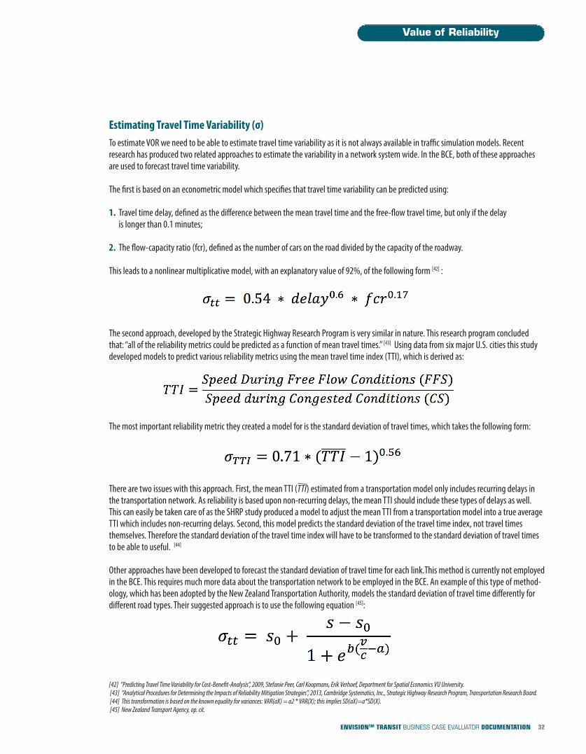
Estimating Travel Time Variability (σ)To estimate VOR we need to be able to estimate travel time variability as it is not always available in traffic simulation models. Recent research has produced two related approaches to estimate the variability in a network system wide. In the BCE, both of these approachesare used to forecast travel time variability.
The first is based on an econometric model which specifies that travel time variability can be predicted using:
1. Travel time delay, defined as the difference between the mean travel time and the free-flow travel time, but only if the delay is longer than 0.1 minutes;
2. The flow-capacity ratio (fcr), defined as the number of cars on the road divided by the capacity of the roadway.
This leads to a nonlinear multiplicative model, with an explanatory value of 92%, of the following form [42] :
The second approach, developed by the Strategic Highway Research Program is very similar in nature. This research program concludedthat: “all of the reliability metrics could be predicted as a function of mean travel times.” [43] Using data from six major U.S. cities this study developed models to predict various reliability metrics using the mean travel time index (TTI), which is derived as:
The most important reliability metric they created a model for is the standard deviation of travel times, which takes the following form:
There are two issues with this approach. First, the mean TTI (TTI) estimated from a transportation model only includes recurring delays inthe transportation network. As reliability is based upon non-recurring delays, the mean TTI should include these types of delays as well.This can easily be taken care of as the SHRP study produced a model to adjust the mean TTI from a transportation model into a true averageTTI which includes non-recurring delays. Second, this model predicts the standard deviation of the travel time index, not travel times themselves. Therefore the standard deviation of the travel time index will have to be transformed to the standard deviation of travel timesto be able to useful. [44]
Other approaches have been developed to forecast the standard deviation of travel time for each link.This method is currently not employedin the BCE. This requires much more data about the transportation network to be employed in the BCE. An example of this type of method-ology, which has been adopted by the New Zealand Transportation Authority, models the standard deviation of travel time differently fordifferent road types. Their suggested approach is to use the following equation [45]:
Value of Reliability
[42] “Predicting Travel Time Variability for Cost-Benefit-Analysis”, 2009, Stefanie Peer, Carl Koopmans, Erik Verhoef, Department for Spatial Economics VU University.[43] “Analytical Procedures for Determining the Impacts of Reliability Mitigation Strategies”, 2013, Cambridge Systematics, Inc., Strategic Highway Research Program, Transportation Research Board.[44] This transformation is based on the known equality for variances: VAR(aX) = a2 * VAR(X); this implies SD(aX)=a*SD(X).[45] New Zealand Transport Agency, op. cit.
32ENVISIONTM TRANSIT BUSINESS CASE EVALUATOR DOCUMENTATION
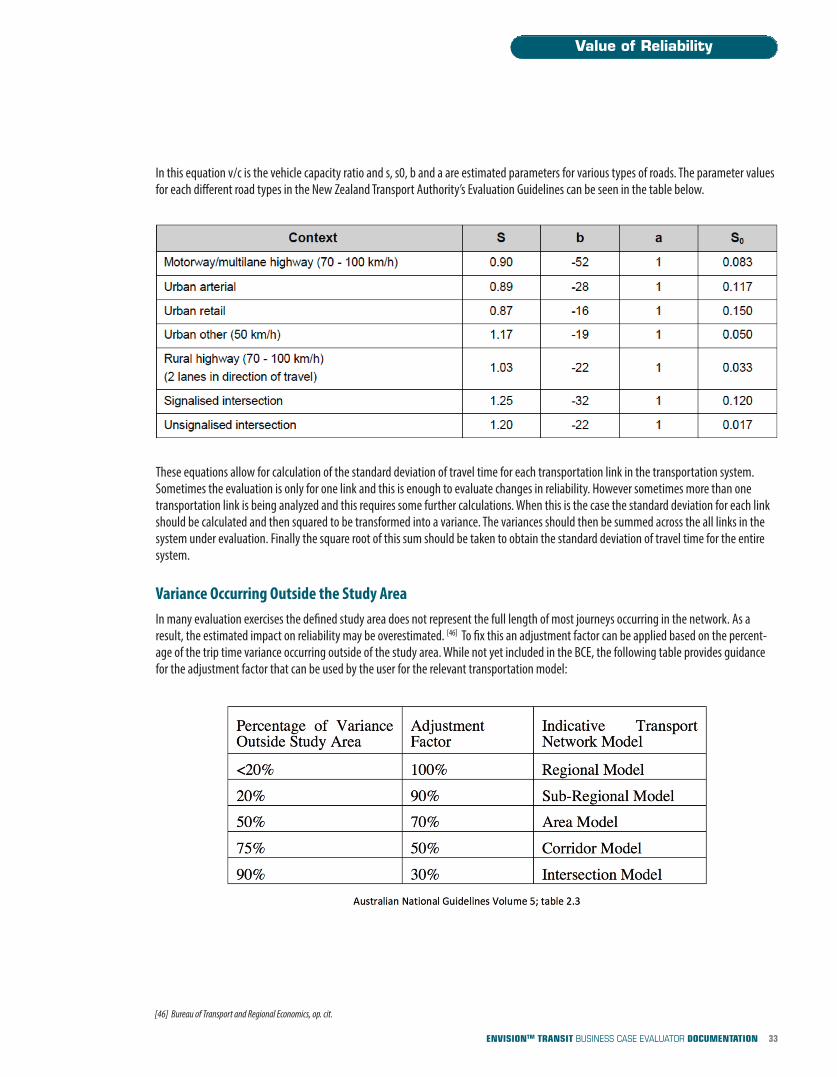
In this equation v/c is the vehicle capacity ratio and s, s0, b and a are estimated parameters for various types of roads. The parameter valuesfor each different road types in the New Zealand Transport Authority’s Evaluation Guidelines can be seen in the table below.
These equations allow for calculation of the standard deviation of travel time for each transportation link in the transportation system.Sometimes the evaluation is only for one link and this is enough to evaluate changes in reliability. However sometimes more than onetransportation link is being analyzed and this requires some further calculations. When this is the case the standard deviation for each linkshould be calculated and then squared to be transformed into a variance. The variances should then be summed across the all links in thesystem under evaluation. Finally the square root of this sum should be taken to obtain the standard deviation of travel time for the entiresystem.
Variance Occurring Outside the Study AreaIn many evaluation exercises the defined study area does not represent the full length of most journeys occurring in the network. As a result, the estimated impact on reliability may be overestimated. [46] To fix this an adjustment factor can be applied based on the percent-age of the trip time variance occurring outside of the study area. While not yet included in the BCE, the following table provides guidancefor the adjustment factor that can be used by the user for the relevant transportation model:
Value of Reliability
[46] Bureau of Transport and Regional Economics, op. cit.
33ENVISIONTM TRANSIT BUSINESS CASE EVALUATOR DOCUMENTATION
Estimation IssuesIn general Stated Preferences methods (SP) – asking people directly about their behavior and preferences in a variety of simulated situations -may be a very poor method for understanding the value of reliability. This is because these methods cause information overload for the respondent. Behavioral economics shows us that people are bad at mental calculations involving probabilities or frequencies – even statisticians don’t find probability intuitive. This implies a psychological bias which pollutes the estimated RR when it is calculated via SP methods as respondents are likely answering a different question in their head than the research was intending to measure. [47] On the otherhand revealed preference methods (RP) – observing people’s actual behavior in certain situations and inferring their preferences - may alsohave a crude estimation of the cost of congestion in the measure for the RR. This would overestimate the RR as congestion has not been explicitly controlled for.
MethodologyThe first step in calculating the VOR is to calculate the relevant statistics, for each hour of the day, needed to forecast the standard deviation oftravel time determinants. These are the delays from free flow speeds, the recurring mean travel time index, and the number of people on theroad, by type (drivers, passengers, and businessmen/women). As the standard deviation of travel time is unknown and its forecast is subjectto uncertainty, both Peer’s (2009) and SHRP’s (2012) methodologies are used to forecast the system wide standard deviation of travel times ineach year. In other words, the BCE’s methodology accounts for the uncertainty in the estimation of this value, as best as the literature allowsfor. To obtain the change in reliability this metric is forecasted for both the base case and the alternative case; the difference between the twois the increase (or decrease) in network reliability.
Once the change in reliability is calculated it needs to be valued for each type of person on the road. This is done by taking the change in reliability and multiplying it by each person’s respective value of time, and the calculated reliability ratio. The reliability ratio used is an average of internationally recommended values at the median, where the range around the median value is calculated from over 30 studies.The final value equates to the VOR in each hour of the day, which is then summed and multiplied by the number of days in a year. Since weekday traffic flows are much greater than weekend traffic flows they are calculated separately to account for these inherent differences.
Components:
n Forecasted traffic flows and congestion levels
n Forecasted standard deviation of travel times
n Reliability ratio
n Value of travel time, by passenger type
Includes: The value of changes in travel time variability
Excludes: The value of changes in the mean travel time, or congestion level
Default Stakeholder Group: 33% User/Target Beneficiary, 33% Community, 33% Economic or Business Activity
Default Envision Categories: 100% Quality of Life
Value of Reliability
[47] “What is the value of reliability”, 2010, Mogens Fosgerau, Centre for Transport Studies Stockholm.
34ENVISIONTM TRANSIT BUSINESS CASE EVALUATOR DOCUMENTATION
Low Income Mobility Benefit
Improving transit service greatly impacts the transportation options of those who have restricted access to transit – those in poverty ornear to poverty. Owning and operating a vehicle, renting a car, or taking a taxi, is typically much more expensive than public transit; therefore transit improvements allow for impoverished people to have improved access to mobility. As stated in the Cost of Congestion report, commissioned by the Greater Toronto Area and Hamilton transit authority Metrolinx:
“Affordable mobility benefits are benefits to low-income households stemming from the availability of transportation at alower price than taxis and more expensive alternatives. Mobility benefits can vary substantially across transit investment type,area and corridor.” [48]
The benefit of increasing basic access to mobility is large as:
“Individuals with access to basic mobility enjoy the benefits of social interaction, entertainment and education which in turninfluences their contribution to society and the economy. And, basic mobility extends the opportunities for employment to indi-viduals who, without this access may otherwise be unemployable. These characteristics of basic mobility, taken together, makea positive contribution to the economy.” [49]
Methodology
To calculate this affordable mobility benefit, we estimate the change in consumer surplus for the low income population due to the transitpolicy. To do this, we first determine the number of low income riders in both the base case and the new transit case. This is accomplishedby taking the percentage of people under the poverty line, and those who are near poor – defined as those under 150% of the poverty line. [50]
Next we determine the mode of transportation they would have taken before based on mode-choice characteristics of poor people in thecity before the transit project. The possible modes of transportation they could have come from are: taxies, driving alone in a private auto,carpooling in a private auto, driving a motorcycle, riding a bicycle, or walking.
Next the associated price of each alternative service is calculated. This is based on the local taxi fares, transit fares, and vehicle operating costs.Given the change in the number of trips, the percent of those trips diverted from each mode, and the associated price of each trip the resultingconsumer surplus is calculated. As the generalized cost of travel for low income users is now lower we can estimate their gain in consumer surplus. This gain in their consumer surplus can also be viewed as the net benefit of increased mobility options for low income users.
Other Possible Benefits
[48] “Costs of Road Congestion in the Greater Toronto and Hamilton Area: Impact and Cost Benefit Analysis of the Metrolinx Draft Regional Transportation Plan”, 2008, John Parker, HDR Corporation Decision Economics, Greater Toronto Transportation Authority, Risk Analysis Investment and Finance Economics and Policy.
[49] “Policy and Planning as Public Choice: Mass Transit in the United States”, 1999, David Lewis, Fred Laurence Williams, United States Department of Transportation.[50] “Life on the Edge: Living Near Poverty in the United States, 1966-2011”, 2012, Misty L. Heggeness, Charles Hokayem, SEHSD Working Paper 2013-02.
35ENVISIONTM TRANSIT BUSINESS CASE EVALUATOR DOCUMENTATION
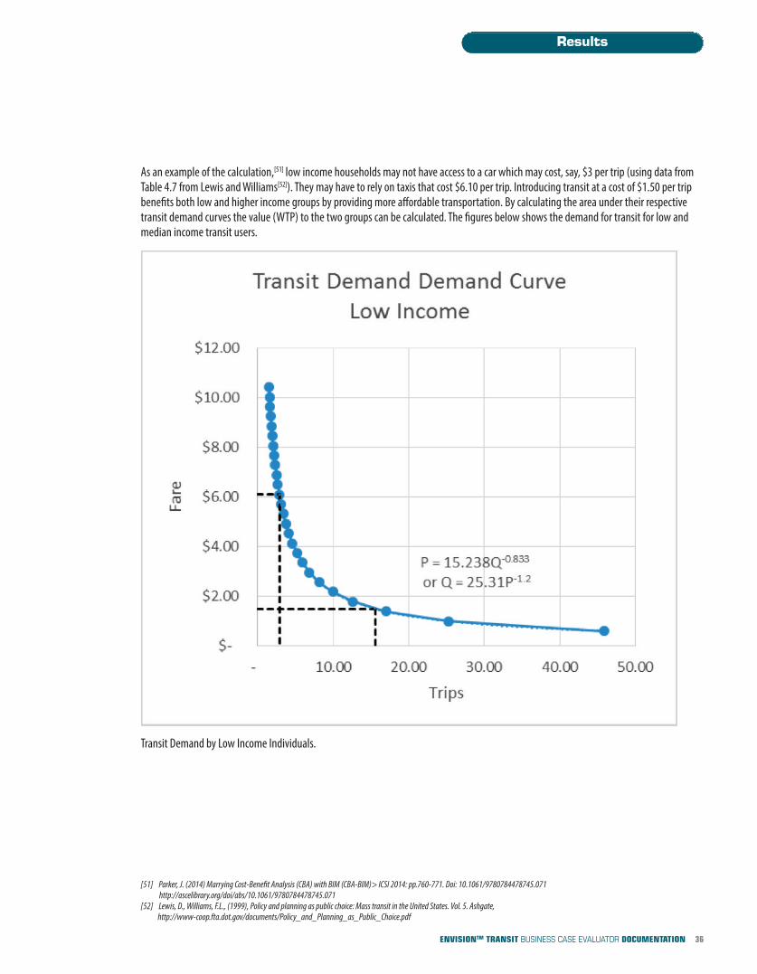
As an example of the calculation,[51] low income households may not have access to a car which may cost, say, $3 per trip (using data fromTable 4.7 from Lewis and Williams[52]). They may have to rely on taxis that cost $6.10 per trip. Introducing transit at a cost of $1.50 per tripbenefits both low and higher income groups by providing more affordable transportation. By calculating the area under their respectivetransit demand curves the value (WTP) to the two groups can be calculated. The figures below shows the demand for transit for low andmedian income transit users.
Transit Demand by Low Income Individuals.
Results
36ENVISIONTM TRANSIT BUSINESS CASE EVALUATOR DOCUMENTATION
[51] Parker, J. (2014) Marrying Cost-Benefit Analysis (CBA) with BIM (CBA-BIM)> ICSI 2014: pp.760-771. Doi: 10.1061/9780784478745.071 http://ascelibrary.org/doi/abs/10.1061/9780784478745.071
[52] Lewis, D., Williams, F.L., (1999), Policy and planning as public choice: Mass transit in the United States. Vol. 5. Ashgate, http://www-coop.fta.dot.gov/documents/Policy_and_Planning_as_Public_Choice.pdf
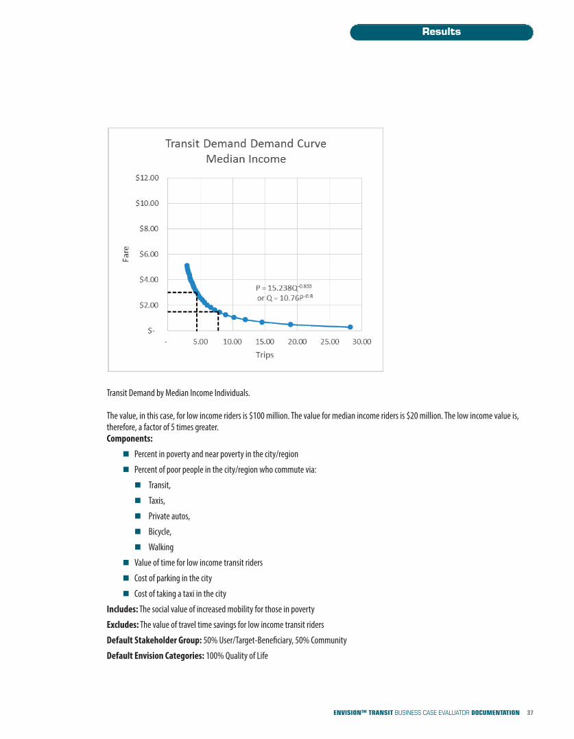
Transit Demand by Median Income Individuals.
The value, in this case, for low income riders is $100 million. The value for median income riders is $20 million. The low income value is,therefore, a factor of 5 times greater.Components:
n Percent in poverty and near poverty in the city/region
n Percent of poor people in the city/region who commute via:
n Transit,
n Taxis,
n Private autos,
n Bicycle,
n Walking
n Value of time for low income transit riders
n Cost of parking in the city
n Cost of taking a taxi in the city
Includes: The social value of increased mobility for those in poverty
Excludes: The value of travel time savings for low income transit riders
Default Stakeholder Group: 50% User/Target-Beneficiary, 50% Community
Default Envision Categories: 100% Quality of Life
Results
37ENVISIONTM TRANSIT BUSINESS CASE EVALUATOR DOCUMENTATION
Ownership – Vehicle Operating CostsAutomobile owners realize lower vehicle operating costs due to transit projects as there is a reduction in the number of vehicle miles travelled (VMT) each day. These variable costs are the use of fuel, the need for oil changes, tire wear, road tolls paid, maintenance and repair, and parking charges. This leads to large benefits for people who switch from driving an automobile to using public transit after the transitimprovement. However, not all possible operating costs are included. The BCE does not include a change in road tolls paid due to a lack ofconsistency across locations in this variable. Furthermore, the BCE does not include a change in parking costs. This is because people who commute via automobile rarely pay the full price of parking; some have subsidized parking, some have free parking, and only a small fraction payfull-price for parking.[53] Without additional information on the distribution of who pays for parking this cannot be incorporated into the model.
Methodology
To calculate the change in vehicle operating costs the BCE first calculates the reduction in VMT by vehicle type. To do this we use the forecasted traffic flow information in the base case and transit case and take the difference in total VMT’s. This is then split between vehicletypes based on the U.S. wide average percent of vehicles which are each type. The types of vehicles included are: small sedans, midsizesedans, large sedans, vans, electric cars, SUV’s, light trucks, and motorcycles. The per VMT cost of operating a vehicle, which includes gasoline expenses, maintenance expenses, and tire expenses, is then calculated. Using this per VMT cost and the change in VMT’s we cannow calculate the final value of the change in operating costs.
Components:
n Change in VMT
n Distribution of vehicles by vehicle type
n Operating costs of vehicles by vehicle type per VMT
Includes: The reduction in the variable costs of driving a vehicle
Excludes: Parking Costs | Toll Costs | Fixed costs of owning a vehicle
Default Stakeholder Group: 33% User/Target Beneficiary, 33% Community, 33% Economic or Business Activity
Default Envision Categories: 100% Resource Allocation
Results
38ENVISIONTM TRANSIT BUSINESS CASE EVALUATOR DOCUMENTATION
[53] “Transportation Cost and Benefit Analysis II – Parking Costs”, 2012, Todd Litman, Victoria Transport Policy Institute.
Ownership – Fixed Vehicle CostsTransit improvements may not only lead to people driving less – it may affect each household’s decision on whether or not to own a car. Ithas been shown that auto ownership is primarily a function of neighborhood density, average per capita incomes, average family size, andthe availability of public transit.[54] Therefore when a transit project increases the availability of public transit, vehicle ownership is reduced.
As car ownership has many fixed costs, such as insurance, the cost of the car, and licensing and registration fees, there are an additionalbenefits to households that decide not to own a car, or to own less cars. However, there is some debate whether or not this benefit shouldbe included in a cost-benefit analysis. The basis of this debate is whether ownership costs are perceived (and lead to a change in consumersurplus), or whether they simply influence behavior (and lead to the change in mode share).[55] This is addressed in a Transit Cooperative Research Program report, sponsored by the Federal Transit Administration which argues:
“Transit improvements affect relatively long-run decisions, including decisions to own motor vehicles. Hence, the relevant demand relationships that should be used in the analysis and the relevant user-cost perceptions that properly belong in theanalysis are long run in perspective. To measure the benefits of a transit improvement, all costs (variable and fixed) should bereduced to unit costs (per vehicle-mile traveled or per trip) and incorporated in the long-run perception of cost.”[56]
This is also the view taken in the BCE and therefore the change in the fixed costs of vehicle ownership are included in the analysis.
Methodology
To calculate the change in fixed costs the BCE uses a model which predicts household vehicle ownership based on household density,household income, people per household, and transit density. Transit density is dependent on the frequency, reach, and type of transit inthe corridor. As this changes between the base case and new transit scenario we can calculate the change in vehicle ownership. Next thetotal number of reduced owned vehicles is broken apart by vehicle type, using the distribution of vehicle types. The same types of vehiclesas used in the vehicle operating costs methodology is used. The value of ownership costs is then estimated for each vehicle type by calculat-ing the average costs of insurance, license, registration, taxes, and finance charges.
Components:
n Vehicles per household
n Population density
n Income per person
n Persons per household
n Transit density before and after the project
Includes: The reduction in fixed costs of driving a vehicle
Excludes: Depreciation of the automobile
Default Stakeholder Group: 33% User/Target Beneficiary, 33% Community, 33% Economic or Business Activity
Default Envision Categories: 100% Resource Allocation
Results
39ENVISIONTM TRANSIT BUSINESS CASE EVALUATOR DOCUMENTATION
[54] “Location Efficiency: Neighborhood and Socio-Economic Characteristics Determine Auto Ownership and Use – Studies in Chicago, Los Angeles and San Fransisco”, 2002, John Holtzclaw, Robert Clear, Hank Dittmar, David Goldstein.
[55] “Estimating the Benefits and Costs of Public Transit Projects: A Guidebook for Practitioners”, 2002, ECONorthwest and Parsons Brinckerhoff Quade & Douglas, Inc., Transit Cooperative Research Program, Federal Transit Administration.
[56] Ibid
Reduced Accident Risk BenefitTransportation accidents, however small or large, impose real costs on society. This risk of accident is heightened if there are more cars onthe road, if those cars travel at faster speeds, and if drivers take to the roads in riskier situations – like a snow storm. Some types of vehiclesimpose different types of risks to society. For instance, the mortality risk of driving a motorcycle is much higher than for a pick-up truck as,when an accident does occur, the motorcyclist has very little protection. In general, people in lighter and smaller vehicles are at a disadvantage when colliding with larger, heavier vehicles.[57] Therefore, these types of vehicles carry a higher risk of injury and mortality. Ingeneral, crashes can be placed in to three broad categories: those that lead to a mortality, those that lead to injuries, and finally those that only lead to property damage. Each of these categories have a different cost to society.
As summarized by the VPTI, the crash risk to each individual for any given trip is low:
"The average motorist has: less than one reported culpable (at fault) vehicle insurance claim per decade, mostly involvingminor property damage; one culpable crash-related claim every 24 years; and one causality crash (causing injury or death) justonce every 62 years. Even high-risk motorists (such as young males) drive most years without a reported culpable crash."[58]
However, the overall risk of a crash is high when considering how many cars are on the road at any given time, and the number of trips people take in their life time. As summarized by the VPTI:
"[C]rash risk is significant and crashes can have catastrophic impacts, causing tens of thousands of deaths, millions of injuries andhundreds of billions in losses annually. In the U.S. Traffic crashes are a leading cause of death among people in the prime of life." [59]
Since the overall risk of a crash happening in the network is high, and the value of individual crashes can be large, even small changes invehicle use can lead to significant crash risk savings.
Methodology
In the BCE, this value is captured using several steps. First the total value of accidents, by vehicle and accident type, in the U.S. is calculated.This is done by taking the average annual number of incidents that have occurred and multiplying each incident by its respective value interms of life, health or property damage. For fatalities, the value used, is the value of a statistical life (VSL), while for injuries a quality-adjusted life year (QALY) approach is employed. These are both explained in more detail below. For property damages, the value is set equalto the average insurance claim for all property damage related incidents in the U.S.. These values are then put into relative terms by divid-ing each value by the VMT, for each vehicle type. This gives us the dollar value of risk per VMT, by vehicle type.
As the transit project leads to a change in VMT’s, we can now assess the change in accident risk using the dollar value of risk per VMT. To assess the change in crash risk by vehicle type, the change in VMT’s needs to be broken apart by vehicle type. To accomplish this the distribution of vehicle types on U.S. roads is used and it is assumed that each type of vehicle, in aggregate, drives the same length.
Components: n Accident statistics by type of injury and type of vehiclen Total VMT in the U.S.n Total miles walked in the U.S.n The change in VMT and miles walked due to the projectn The distribution of traffic by vehicle type
Includes: The social value of reducing accidents and accident risk
Excludes: The value of reduced stress due to reduced accident risk
Default Stakeholder Group: 50% User/Target-Beneficiary, 50% Government
Default Envision Categories: 100% Quality of Life
Results
40ENVISIONTM TRANSIT BUSINESS CASE EVALUATOR DOCUMENTATION
[57] “Fatality Facts”, 2013, Insurance Institute for Highway Safety Highway Loss Data Institute.[58] “Transportation Cost and Benefit Analysis II – Safety and Health Costs”, 2012, Todd Litman, Victoria Transport Policy Institute.[59] Ibid
Value of Statistical LifeEconomists use the value of a statistical life (VSL), or less commonly, value of mortality risk, when analyzing the risk and reward trade-offspeople make. As defined by the U.S. Department of Transportation:
“The benefit of preventing a fatality is measured by what is conventionally called the [VSL], defined as the additional cost thatindividuals would be willing to bear for improvements in safety (that is, reductions in risks) that, in the aggregate, reduce theexpected number of fatalities by one.” [60]
It is important to highlight the fact that the VSL is not intended to be the value of a specific life. It is the value placed on changes in the likelihood of death, not the price someone would pay to avoid death. In the BCE, we do not place a dollar value on individual lives. Rather,when conducting a benefit-cost analysis of infrastructure we use estimates of how much people are willing to pay for small reductions intheir risks of dying from adverse health conditions that may be caused or improved by the infrastructure.
The Value of a Statistical Life seems to be widely used in the regulatory impact analysis and cost benefit studies for federal government costbenefit analyses (e.g. safety improvements in rail and roadways). A range of $5-$13 million with a median around $9 million seems to beaccepted. These values are in 2012 U.S. Dollars and are adjusted for inflation depending on the year they are realized.
Economists often estimate the VSL by looking at the risks that people take or say they will take and how much they are or must be paid fortaking them. These studies are called revealed preference studies. Jobs with greater risk of death are often compensated with higher wages.By statistically controlling for other job characteristics a hedonic wage model can determine the value of the extra risk that is compensatedfor in the wage. Another method to estimate the VSL is to survey them on their willingness to pay for a reduction in the likelihood of death,perhaps through safety improvements or more stringent standards. These types of studies are called stated preference studies.
In general the VSL literature suggests that the VSL increases with real incomes, however the exact rate of increase is subject to debate. Therate of increase is dependent on the income-elasticity of VSL; defined as the percentage increase in the VSL for a percentage increase in income. The main point of contention is whether or not the VSL increase proportionately with incomes, and if it does not, whether mortalityrisk be thought of as a luxury good.[61],[62] If mortality risk were to be a luxury good it would imply that as a person’s wants are better satis-fied, they begin to place a relatively higher value of health and longevity. This is the view the literature appears to support. However, as the debate in the literature is on-going, the U.S. DOT recommends that the VSL should increase proportionately with income.[63] As the Congressional Budget Office has forecasted real median wages to grow at an annualized rate of 1.18% this implies the VSL should also increase at this rate.[64] This is the method used in the BCE.
It is important to point out that the U.S. DOT recommends a single nationwide value be used regardless of age, income, socioeconomic status,mode of travel, location, or the nature of the risk.[65] That is no adjustment should be made to reflect differences in the local population.
As non-fatal injuries are far more common than fatalities in traffic accidents the U.S. DOT has also provided recommendations on calculatedthe value of these injuries. These estimates are based on the type of accidental injury, grouped by the Abbreviated Injury Scale (AIS), whichmeasures the injuries severity and duration. To assign a value to each AIS group, a scale known as the quality-adjusted life years (QALYs) isused to compare the injury to the alternative of perfect health.[66] The quality-adjusted life year measures of the burden of a disease or in-jury, including both the quality and the quantity of life lived. Put differently, QALY’s account for both changes in the expected lifespan of a person, and changes in the quality of a person’s life even if their expected lifespan remains unchanged. This methodology provides a coefficient for each AIS group of injury that can be applied to the VSL to assign a final value for each injury class. In other words, the value of an injury can also be thought of as the value of a fraction of a fatality, and the fraction used is derived using QALY’s.
Results
41ENVISIONTM TRANSIT BUSINESS CASE EVALUATOR DOCUMENTATION
[60] “Treatment of the Value of Preventing Fatalities and Injuries in Preparing Economic Analyses”, 2014, Jack Wells, Office of the Secretary of Transportation, United States Department of Transportation.[61] “The Income Elasticity of the Value per Statistical Life: Transferring Estimates between High and Low Income Populations”, 2011, James Hammitt, Lisa Robinson, Journal of Benefit-Cost Analysis.[62] A luxury good is defined as having an income elasticity greater than 1, which implies that demand increases more than proportionally as incomes rise. [63] That is, the income-elasticity is equal to 1, implying a 1% increase in incomes leads to a 1% increase in the VSL. [64] Jack Wells, op. cit.[65] Jack Wells, op. cit.[66] Jack Wells, op. cit.
Air Pollution & CO2 Emissions ReductionAutomobiles and transit vehicles are a major source of both greenhouse gases (GHG’s), which have the potential to warm the planet to unstable levels, and criteria air contaminants (CAC’s), which lead to issues such as smog and acid rain. GHG’s typically refer to carbon dioxide(CO2), methane (CH4), and nitrous oxide (N2O) and each have a different global warming potential (GWP). In the U.S., automobile use accounts for 29% of total GHG’s.[67] CAC’s refer to sulphur oxides (SOx), nitrogen oxides (NOx), particulate matter (PM), volatile organic compounds (VOC), carbon monoxide (CO), and ammonia (NH3). With regards to CAC’s the EPA estimates that:
“[M]otor vehicles are responsible for nearly one half of smog-forming volatile organic compounds (VOCs), more than half of the nitrogen oxide (NOx) emissions, and about half of the toxic air pollutant emissions in the United States. Motor vehicles, including non-road vehicles, now account for 75 percent of carbon monoxide emissions nationwide.” [68]
Therefore reducing motor vehicle use, and thus fuel consumption, can lead to large environmental benefits. As stated by the NHTSA:
“Reducing fuel consumption also lowers the economic costs of environmental externalities resulting from fuel production anduse, including reducing the impacts on human health impacts from emissions of criteria air pollutants, and reducing futureeconomic damages from potential changes in the global climate caused by greenhouse gas emissions.” [69]
The change in CAC’s and GHG’s can be captured through several different types of models. Some transportation models estimate the changein air pollution directly in the model. If this is the case, these projected changes will be incorporated and valued in the BCE. If the transportation model the user analyzed their transit project with did not incorporate air pollution directly in the model, there are two otheroptions. First, the user could utilize the Environmental Protection Agency’s (EPA) Motor Vehicle Emission Simulator (MOVES) to estimatethe change in air pollution due to a reduction in automobile use.[70] The last alternative is to allow the BCE to estimate the change in air pollution directly. If this method is chosen the estimate will be based on any changes in vehicle miles travelled, and any changes in energyusage. This methodology uses estimates from the EPA on per VMT emissions of CAC’s and GHG’s, by vehicle type.
Results
42ENVISIONTM TRANSIT BUSINESS CASE EVALUATOR DOCUMENTATION
[67] “Transportation’s Role in Reducing U.S. Greenhouse Gas Emissions”, 2010, Center for Climate Change and Environmental Forecasting, United States Department of Transportation. [68] “Cars, Trucks, Buses, and "Nonroad" Equipment”, 2014, EPA.[69] “Damages per tonne emission of PM2.5, NH3, NOx and VOCs from each EU25 Member State (excluding Cyprus) and surrounding seas”, 2005, Mike Holland, Steve Pye, Paul Watkiss,
Bert Droste-Franke, Peter Bickel, Clean Air for Europe (CAFE) Programme.[70] “MOVES (Motor Vehicle Emission Simulator)”, 2015, EPA.
MethodologyTo estimate the value of reduced CAC’s we apply the social cost of each air pollution to the calculated reduction in tonnes of each pollutant,in each year. This social cost is based on the impact each pollutant, per tonne, causes to human health, agriculture, buildings, and the localecology. This is done through what is known as the damage function approach – which relies on the principle that changes in CAC’s lead tostatistically significant changes in health, agricultural, and ecological outcomes. What is included in each of these functions is dependenton the type of pollutant. For instance, some pollutants, like PM2.5, can travel very far distances and can cause damages to agriculturallands that are not close to the source of pollution. On the other hand, other pollutants are much more local and would not include agricul-tural damages in these functions. The specific values used are, at the median, are the U.S. DOT recommended values and risk ranges havebeen placed around these values based on a literature review containing more than 400 estimates across all CAC’s.
To estimate the value of reduced GHG’s the BCE first adjusts each GHG to its carbon dioxide equivalent (CO2e) using its estimated GWP. Thenthe social cost of carbon is used to value the change in total tonnes of CO2e due to the project. The social cost of carbon used follows theU.S.’s Interagency Working Group on the Social Cost of Carbon guidelines with an additional range placed around this recommended valueusing estimates from the literature on the economic impacts of global warming.
Components:
n Carbon and pollution intensities of motor vehicles
n CO2e conversion factors
n Forecasted carbon emissions
n Social Cost of Carbon (see Appendix C)
n Social Cost of CAC’s (see Appendix C)
Includes: Reduced carbon emissions due to reduced vehicle miles traveled | Increased carbon sequestration due to trees | Health, climate,environmental, and damage components of the social cost of carbon and CAC’s.
Excludes: Reduced carbon emissions and CAC’s due to reduced car ownership (embodied energy and upstream pollution).
Default Stakeholder Group:
Carbon Emissions → 100% Environmental
Air Pollution → 50% Community, 50% Environmental
Default Envision Categories:
Carbon Emissions → 100% Climate
Air Pollution → 33% Natural World, 33% Quality of Life, 33% Climate
Results
43ENVISIONTM TRANSIT BUSINESS CASE EVALUATOR DOCUMENTATION
Noise Pollution ReductionNoise pollution refers to the noise emitted by vehicles on roadways and can be thought of as unwanted sounds and vibrations. Motor vehicles produce various types of noise caused by: engine acceleration, tire contact with the road, horns, and car alarms designed to preventtheft. Heavier vehicles also cause vibrations, or low frequency noise. According to the OECD, “Transport is by far the major source of noise,ahead of building or industry, with road traffic being the chief offender.” [71]
The World Health Organization (WHO) lists noise as a major environmental issue in urban areas which affects a large number of people.Until recent years the impact of noise on human health focused on its impact on levels of annoyance. However, in recent years, a large bodyof evidence has been amassed studying the health impacts of noise. The WHO deems the following health outcomes to have a causal link to changing noise levels:
n Cardiovascular diseases:
“Road traffic noise has been shown to increase the risk of ischaemic heart disease, including myocardial infarction. Both roadtraffic noise and aircraft noise increase the risk of high blood pressure.”[72]
n Cognitive impairment of school aged children:
“Over 20 studies have shown negative effects of noise on reading and memory in children….” [73]
n Sleep disturbance:
“Environmental noise may reduce the restorative power of sleep by means of…sleep fragmentation…Acute and chronic sleeprestriction or fragmentation has been shown to affect…waking psychomotor performance, memory consolidation, creativity, risk-taking behaviour, signal detection performance and risks of accidents.” [74]
n Tinnitus [75]
n Annoyance [76]
In general there are two methods for calculating the impact of noise. The first, developed in the 1997 Federal Highway Cost AllocationStudy by the Federal Highway Association, a division of the U.S. Department of Transportation estimates:
“Noise costs [are estimated] using information on the reduction in residential property values caused by noise emissions ofhighway vehicles.” [77]
Results
44ENVISIONTM TRANSIT BUSINESS CASE EVALUATOR DOCUMENTATION
[71] “Environmental Policies for Cities in the 1990s”, 1990, OECD (www.oecd.org), cited in Poldy, p.29.[72] “Burden of disease from environmental noise: Quantification of healthy life years lost in Europe,” 2011, World Health Organization.[73] Ibid.[74] Ibid.[75] Ibid.[76] Ibid.[77] “Federal Highway Cost Allocation Study”, 1997, United States Department of Transportation.
The second incorporates directly estimates the health benefits due to reduced cardiovascular disease risk, increased cognitive ability, reduced sleep disturbance, reduced prevalence of Tinnitus, and reduced annoyance levels. This is a more direct method to analyze the negative externality of noise. Furthermore, for property prices to fully capitalize all of these negative health benefits, the impact of noise onhuman health would have to be highly salient. As the impact of noise on health occurs in small amounts, over long time horizons, it is unlikely that the full value of noise impacts is capitalized in housing prices. Therefore, the framework employed in the BCE does not rely onthe impact on property prices.
Methodology
The BCE uses a study from the European Union (EU) which documents the value per kilometer travelled decomposed by type of vehicle,time of day, and whether the project is in an urban, suburban or rural area. This study is based on a report from the World Health Organization(WHO) which documents the health impacts of noise, and a dose-response study which evaluates the impacts of varying levels of noise onvarious diseases. Combining these two studies, the value of noise per mile is estimated based on the reduction in morbidity using the QALYmethodology. In the BCE this is applied by first determining the reduction in VMT’s by vehicle type, whether the reduction is occurring dur-ing the day or night, and whether the area is urban, suburban, or rural. The value from the EU study is then converted to a USD per milemetric which can be applied to this reduction in VMT’s. Using the change in VMT’s and the dollar value of noise pollution per VMT allows usto estimate the final value of noise pollution.
Components:
n Change in VMT’s, by vehicle type
n Distribution of traffic by night and day
n Population density of the city/region
n Euro to USD exchange rate
Includes: The social value of noise pollution and the impacts of noise on human health
Excludes: The value of noise on property values | The ecological impacts of noise pollution
Default Stakeholder Group: 50% Community, 50% Government
Default Envision Categories: 100% Quality of Life
Results
45ENVISIONTM TRANSIT BUSINESS CASE EVALUATOR DOCUMENTATION
Oil Consumption ExternalityResource externalities refer to the externalities caused through oil dependency and use. If a transit project decreases automobile use, and thedemand for oil, then this implies there will be a reduction in oil imports, and domestic oil extraction. Impact Infrastructure has considered fourresource externalities for the BCE. They are: monopsony costs, macroeconomic exposure to oil shocks, costs of maintaining a military presence infragile oil producing regions, and the environmental cost incurred from oil spills. These are each explained below.
1) Monopsony Costs:
These refer to the higher prices for petroleum products that result from the effect that U.S. oil import demand has on the world oil price.These costs are explained by the National Highway Traffic Safety Administration (NHTSA):
“Increased U.S. petroleum consumption can impose higher costs on all purchasers of petroleum products, because the U.S. is asufficiently large purchaser of foreign oil supplies that changes in U.S. demand can affect the world petroleum price. The effectof U.S. petroleum demand on world oil prices is determined by the degree of OPEC monopoly power over global oil supplies, andthe degree of monopsony power over world oil demand that the U.S. exercises. [… Therefore] reducing U.S. oil imports canlower the world petroleum price, and thus generate benefits to other oil purchasers by reducing these ‘monopsony costs.’” [78]
While estimates do exist on the value of these costs to the U.S. economy, they are not included in the BCE. This is because, as argued by theNHTSA, that this is not an externality but is rather a global transfer of wealth from oil exporters to oil importers.[79] In other words it represents a financial transfer of real cash and does not imply a change in the use of real economic resources, nor does it lead to a change in neither consumer nor producer welfare.
2) Macroeconomic Exposure to Oil Shocks:
This refers to the external economic cost imposed by imports of petroleum into the U.S. that arises from an increase in oil prices triggered by a disruption in the supply of imported oil. This reduces the level of output that can be produced in the U.S. economy. This type of macroeconomicshock is explained by the NHTSA:
“Since future disruptions in foreign oil supplies are an uncertain prospect, each of these disruption costs must be adjusted bythe probability that the supply of imported oil to the U.S. will actually be disrupted. The “expected value” of these costs – theproduct of the probability that an oil import disruption will occur and the costs of reduced economic output and abrupt adjust-ment to sharply higher petroleum prices – is the appropriate measure of their magnitude. Any reduction in the expected valueof these costs resulting from a measure that lowers U.S. oil imports represents an additional benefit to the U.S. economy be-yond the direct value of savings from reduced purchases of petroleum products.” [80]
Since reducing demand for automobile travel leads to a reduction in U.S. oil imports this external economic cost can be viewed as a benefit,and not simply a transfer of wealth. Therefore this benefit is included in the resource externality benefit calculation.
Results
46ENVISIONTM TRANSIT BUSINESS CASE EVALUATOR DOCUMENTATION
[78] “Corporate Average Fuel Economy for MY 2017- MY 2025 Passenger Cars and Light Trucks”, 2012, Office of Regulatory Analysis and Evaluation National Center for Statistics and Analysis, National Highway Traffic Safety Administration.
[79] Ibid.[80] Ibid.
3) Costs of Maintaining a Military Presence:This cost refers to the external economic cost of maintaining a military presence to secure the supply of oil from countries and regionswhich are potentially unstable. Under the view that the U.S. military will seek to spend money to protect against the interruption of theglobal oil supply, then this is an economic externality and should be included in the analysis. However, the NHTSA states:
“[…] while costs for U.S. military security may vary over time in response to long-term changes in the actual level of oil imports into the U.S., these costs are unlikely to decline in response to any reduction in U.S. oil imports. […] U.S. military activities in regions that represent vital sources of oil imports also serve a broader range of security and foreign policy objectives than simply protecting oil supplies, and as a consequence are unlikely to vary significantly in response to changes in the level of oil imports” [81]
This is not simply the view of the NHTSA as:
“The American Petroleum Institute commented that military expenditures will not likely change with a reduction in U.S. oil imports, and therefore should not be included in the assessment of this rulemaking.” [82]
4) The Environmental Costs of Oil Spills:
This externality refers to the environmental damage caused by oil extraction when there are oil spills and leakages. Theoretically, if the demand for oil were reduced then there would be a reduction in the number of these types of incidents. It’s important to point out that partof these costs are internalized when the party responsible for the damages pays for the clean-up. This implies that there would only be aneconomic benefit if society’s willingness to pay to avoid these environmental damages is higher than the clean-up costs.
While this is a true externality, it has not been considered by the U.S. DOT, the NHTSA, or the EPA. This may be due to the difficulty in separating out the difference between the WTP to avoid these disasters and their clean-up costs. Only one value for this exists in the literature, from the Victoria Policy Transportation Institute (VPTI), however the estimate is based on too many assumptions to be includedin the BCE.[83] If better research becomes available for this benefit, it will be included in future iterations of the BCE.
MethodologyThe only external economic cost imposed by U.S. petroleum imports included in the BCE is the reduced macroeconomic exposure due to oilshocks. The first step to calculate this benefit is to forecast the average miles per gallon for all vehicles on the roads in the U.S. This forecastis based on data in the U.S. DOT NHTSA CAFÉ regulation. Using this value for miles per gallon and the change in VMT’s we can then calculatethe reduction in gallons of fuel consumed. Then using the estimated value of macroeconomic shock risk per gallon of fuel consumed we cancalculate this benefits total value. The first step in calculating the value of reduced risk per gallon is linking the reduction in U.S. petroleumimports to each gallon of fuel saved. Then the expected costs of an oil supply disruptions are calculated for various levels of imports. Basedon these results the macroeconomic risk per gallon of fuel use is determined.
Components:
n The reduction in VMT’s
n The average miles per gallon of the U.S. automobile fleet
n The expected value of macroeconomic risk per gallon of fuel consumed
Includes: The external economic cost due to the risk of oil supply interruptions
Excludes: Monopsony costs | The costs of maintaining a military presence in oil producing countries | The environmental cost of oil an spill
Default Stakeholder Group: 100% Economic or Business Activity
Default Envision Categories: 100% Resource Allocation
Results
47ENVISIONTM TRANSIT BUSINESS CASE EVALUATOR DOCUMENTATION
[81] Ibid.[82] Ibid.[83] “Transportation Cost and Benefit Analysis II – Resource Consumption External Costs”, 2012, Todd Litman, Victoria Transport Policy Institute.
Avoided Road Facilities CostsThis benefit calculates the savings to the transportation authority in terms of reduced roadway costs due to a reduction in vehicle travel onroadways. This value includes the reduced need for new construction (roadway expansion) and O&M costs. Roadway costs not borne by usercharges, such as special fuel taxes, vehicle registration taxes and road tolls are considered external costs. To avoid double counting with vehicle operating costs, only the external portion of these roadway costs are included in the calculation of this benefit. The external roadway facility cost varies by vehicle type as heavier vehicle type’s cause more damage to roadways and the drivers of different vehiclestypes are subject to different user charges.
Methodology
To calculate this benefit we take the calculated change in VMTs by vehicle type and value the external value for each vehicle type. The valueis based on whether the project is in an urban or rural location, the weight of the vehicle, and the percent of the cost that is internalizedthrough user charges. The weight of the vehicle is important as heavier vehicles cause more damages than lighter vehicles, and are thussubject to higher roadway facility costs. A per-VMT cost for each vehicle class is calculated using the damage different weight class’s causeto roadways. As these are external costs, we must also calculate the amount of these facility costs that are covered by user charges by vehi-cle type. For instance, electric cars pay less internal costs as they are subsidized and are not subject to the gasoline tax, therefore their costper VMT is higher than the average gasoline car, all else equal.
Components:
n Population density
n Distribution of vehicle traffic, by vehicle type
n Percent of roadway facility costs that are internal, by vehicle type
n External roadway facility cost, per VMT, by vehicle type
Includes: The change in public expenditures on roadway facilities
Excludes: Roadway costs paid for by vehicle user charges
Default Stakeholder Group: 100% Government
Default Envision Categories: 100% Resource Allocation
Results
48ENVISIONTM TRANSIT BUSINESS CASE EVALUATOR DOCUMENTATION
Personal & Social Value of Active TransportationActive transportation refers to transportation that is muscle powered. This type of transportation involves physical activity such as walking,cycling, roller blading, etc. As physical activity has a major effect on health, active transportation is seen as a cost-effective way to improvepublic health. The VPTI explains the importance of physical activity:
"Inadequate physical activity, and [the] resulting excessive body weight, contribute to various health problems including heart andvascular diseases, strokes, diabetes, hypertensive diseases, osteoporosis, joint and back problems, colon and breast cancers, and depression. More active transport appears to reduce long-term cognitive decline and dementia. Cardiovascular diseases are the leading causes of premature death and disability in developed countries, causing ten times as many lost years of productive life asroad crashes. Even modest reductions in these illnesses can provide large health benefits." [84]
Transit projects can have large health benefits, as increases in transit ridership typically lead to an increase in walking, or other active transporation, for those who switch to commuting on transit rather than by automobile. Furthermore if the transit improvement leads tomore transit-oriented-development then there may be a secondary effect on walking. As people live in denser, multi-modal, walkableneighborhoods, they are more likely to walk to complete their daily tasks. In other words, transit improvements can increase the demandfor walking. Walking is not the only activity demand may change for however, creating multi-modal networks may lead to more peoplechoosing to bicycle to work, for pleasure, or to run errands.
The benefits of active transportation can be thought of as falling into two separate categories, based on who the benefit accrues to. Part of the value of increased health accrues to the individual as they experience a higher quality of life, and live longer. This is known as the personal value of active transportation. On the other hand some benefits of being physically active may accrue to other parties. For instance, if being physically active makes you a more productive worker, or if you're medical bills later in life are lowered, your employer, or government/health insurer, receives a benefit. This is known as the social value of active transportation.
Results
49ENVISIONTM TRANSIT BUSINESS CASE EVALUATOR DOCUMENTATION
[84] “Transportation Cost and Benefit Analysis II – Safety and Health Costs”, 2012, Todd Litman, Victoria Transport Policy Analysis.
Methodology
The first step in calculating the benefits of active transportation requires calculating the change in miles walked or cycled. For walking thisis done in two ways. First the BCE calculates any implied changes in miles walked for those who switch from taking private automobiles totransit. Second if the user inputs any additional changes in miles walked, these are added to the calculation. For cycling, the change inmiles cycled is only included if the user inputs it directly. These changes are then valued based on the health benefits per mile walked, ormile cycled, in terms of reduced disease risk and reduced mortality risk from the literature. Finally this is split between the personal, or internal portion of the benefit, and the social, or external portion of the benefit.
Components:
n Change in miles walked and cycled
n Value of reduced morbidity due to increased activity
n Value of reduced mortality due to increased activity
n Percent of benefit that is social vs. personal
Includes: The health benefits of walking or cycling
Excludes: Changes in the accident risk due to increases in walking or cycling | Changes in the perception of safety when walking or cycling
Default Stakeholder Group:
Personal Value of Active Transportation → 100% User/Target-Beneficiary
Social Value of Active Transportation → 50% Community, 50% Government
Default Envision Categories:
Personal Value of Active Transportation → 100% Quality of Life
Social Value of Active Transportation → 100% Quality of Life
Results
50ENVISIONTM TRANSIT BUSINESS CASE EVALUATOR DOCUMENTATION
iii
Perception of Safety BenefitThe perception of safety benefit, also known as the barrier effect, represents the costs due to the delays that motorized traffic on roadwaysimpose on non-motorized traffic. As explained by the VPTI:
“Damages resulting when motorists hit pedestrians and cyclists are considered accident costs, but not costs people bear whenthey change route or mode to avoid crash risk.” [85]
In general, this benefit captures the change in costs that automobiles impose on pedestrians and cyclists in terms of delays, discomfort,psychological fear of accidents, changes in route choice, and lack of access to specific locations. In other words, motor traffic can be thoughtof as creating a barrier which dampens demand for walking and cycling, and changes the decisions of those who walk and cycle. In the longrun, reducing this barrier leads to a change in consumer welfare.
Methodology
To capture this benefit in the BCE we first calculate the change in VMT’s, by vehicle class. Then we determine the value of a reduction perVMT with regards to reduced barriers to non-motorized travel, by vehicle class. In the literature this is done by first calculating the barrierfactor which is dependent on traffic volumes, average speeds, the share of vehicles which are large vehicles, and the number of pedestriancrossings. Then the demand for crossing is calculated, with and without a barrier, based on the residential, commercial, recreational, andmunicipal destinations within walking, or cycling, distance of the road. From this the change in consumer welfare is calculated due to asmall change in VMT’s for varying vehicle classes. This gives us the barrier cost per VMT by vehicle type which we then use to calculate thefinal value of the perception of safety benefit. The literature supports the view that this value should be different in urban peak, urban off-peak, and rural conditions due to different behavioral responses in each of these settings. Therefore the value used depends on whetherthe change in VMT’s are taking place in an urban or rural setting and whether or not they occur during peak hours, or off-peak hours.
Components:
n The change in VMT’s, by vehicle type, and the time of the day
n The cost per VMT, by vehicle type
n Population density
Includes: The value of perceived safety when walking and cycling and lost consumer surplus due to heavy roadway traffic
Excludes: The health benefits of walking or cycling
Default Stakeholder Group: 50% User/Target-Beneficiary, 50% Community
Default Envision Categories: 100% Quality of Life
Results
51ENVISIONTM TRANSIT BUSINESS CASE EVALUATOR DOCUMENTATION
[85] “Transportation Cost and Benefit Analysis II – Barrier Effect”, 2012, Todd Litman, Victoria Transport Policy Institute.
Property Value UpliftThe property uplift benefit estimates the rise in property values as a result of new or improved transit. Many empirical studies provide evidence that house prices increase with transit investments. These studies estimate the change in the property’s value as measured by theproperties shadow price which is defined as the marginal rate of substitution between housing and non-durable goods. This approach captures the welfare benefit to a household of changing housing prices due to a transit investment. The empirical modelling of transit’s effect on property prices is summarized in Debrezion et. al..[86]
While it is clear that transit has an effect on property prices, it is less clear whether or not the increase in property prices should be viewedas an incremental benefit. Many argue that higher property prices are primarily a capitalization of travel time savings for the property owners who are also transit users. In other words, the property price uplift and travel time savings benefit are the one and the same and including them both would be double counting.[87] This is the view taken by many economists and transit authorities. However, this view ignores the value of non-user benefits.
Non-user benefits are due to changes in the character and form of the neighborhood caused by new or improved transit service. Transit creates new opportunities in neighborhoods and this value may not be fully captured by the intensity of use of the transit system. This isbecause transit enables the opportunity to travel and receive more visits from friends and relatives, and transit stations are frequently localcommercial centers offering new services to the community. These benefits accrue to the neighborhood regardless of transit use and if people value these benefits then property values should reflect their change in the willingness to pay to live in the neighborhood.[88]
There is evidence that the observed willingness to pay to live closer to a transit station most likely includes non-user benefits that propagate from proximity to transit. The easiest way to see that non-user benefits exist is by the fact that many people who live near transitpay a property price premium yet they never use the transit system. Furthermore, there have been empirical attempts to disentangle thechange in property prices from travel time savings to determine how much of this property price increase can be viewed as a non-user benefit. These estimates have found that the property value premium is too large to be explained solely by user benefits. In fact, the resultsfrom property price models exceed the value of travel time saving by up to 50%.[89] In other words as much as 50% of the property priceuplift has been estimated to be non-user benefits.
This methodology has been used in several cost-benefit analyses in North America, including the analysis of the Greater Toronto Area transportation plan. This report argued that the property price effect, over and above the effects of travel time savings, represent the non-user benefits of transit due to transit-oriented development.[90] This report argued that the urbanization and locational attributes thatcan be associated with transit extend beyond the use of the transit system and this value can be captured through property prices. To dothis, the authors followed the above results and estimated non-user benefits as 50% of the property value uplift.
We follow this practice in the BCE and take 50% of the estimated property price increase due to transit as being incremental to the traveltime savings that are capitalized into the other 50% of the property price increase. So, we break the property price increase into two equalhalves representing the user and non-user benefits. The user benefit portion of the property price increase is the same as the travel timesavings benefit and is not included in the analysis. The non-user benefit portion of the property price is due to transit-oriented development and is treated as an incremental benefit.
Results
52ENVISIONTM TRANSIT BUSINESS CASE EVALUATOR DOCUMENTATION
[86] “The Impact of Railway Stations on Residential and Commercial Property Value: A Meta-analysis”, 2007, Ghebreegziabiher Debrezion, Eric Pels, Piet Rietveld, Journal of Real Estate and Financial Economics.
[87] “Cost-benefit analysis: Theory and application”, 1996, Tevfik Nas, Sage Publications.[88] “Measuring the neighborhood benefits of rail transit accessibility”, 1997, Lewis-Workman, S., Brod, D., Transportation Research Record, Journal of the Transportation Research Board.[89] “Policy and Planning as Public Choice: Mass Transit in the United States”, 1999, David Lewis, Fred Laurence Williams, United States Department of Transportation. & “Measuring the
neighborhood benefits of rail transit accessibility”, 1997, Lewis-Workman, S., Brod, D., Transportation Research Record, Journal of the Transportation Research Board.[90] “Costs of Road Congestion in the Greater Toronto and Hamilton Area: Impact and Cost Benefit Analysis of the Metrolinx Draft Regional Transportation Plan”, 2008,
HDR Corporation Decision Economics, Greater Toronto Transportation Authority, Risk Analysis Investment and Finance Economics and Policy
Methodology
The methodology for calculating the property uplift relies on a meta-analysis of the impact of transit stations on residential property values.[91] Based on this study the property value uplift is higher, the closer the property is to the transit station. Furthermore, if the prop-erty already had equal access to transit, or close accessibility to a highway the impact on property values is decreased. Finally, the change inproperty values is dependent on the type of transit investment; commuter rail stations have the largest impact, whereas bus rapid transitstations have the smallest impact. To ensure that this benefit is only accounting for non-user benefits, the estimate impact on property values is then multiplied by 50%.
Components:
n Number of properties within 400, 800, and 1200 meters (approximately 1/4, 1/2, and 3/4 mile) of the transit station
n The average value of all properties in the city
n The accessibility of those properties to highways
n The type of transit being installed
Includes: The non-user benefits of property value increases
Excludes:Value of Travel Time Savings | User Benefits of Transit
Default Stakeholder Group: 100% Community or Other
Default Envision Category: 100% Other
Results
53ENVISIONTM TRANSIT BUSINESS CASE EVALUATOR DOCUMENTATION
[91] “The Impact of Railway Stations on Residential and Commercial Property Value: A Meta-analysis”, 2007, Ghebreegziabiher Debrezion, Eric Pels, Piet Rietveld, Journal of Real Estate and Financial Economics.
Shadow Wage BenefitThe Shadow Wage Benefit represents the poverty reduction benefits of increased local employment opportunities. A recommended approach is tocalculate the social opportunity cost of labour (SOCL) and subtract this from the total wage bill for the project. One way to do this is proposed byShaffer, M.'s Multiple Account Benefit-Cost Analysis book[92] which suggests an equation of: SOCL = pu * vu + (1-pu) * FW, where SOCL is the so-cial opportunity cost of labour, pu is the probability of hiring an unemployed person, vu is the value of what the unemployed persons would other-wise would be doing (this can be thought of as the minimum they would have to be paid to willingly work at the new job), and FW is the financial(or market) wage. Therefore the shadow wage benefit results in an equation of: NB = FW – SOCL = pu * (FW- vu). Here you can see that the Net Benefit (NB) to society will be greater as a result of an increase in employment generated by a project or policy. This is because an increase in employment may lead to hiring more people from a pool of unemployed individuals, which creates value because the wages paid in their new jobs(FW) are greater than what they would otherwise be doing (vu). It is important to note that this benefit will be relatively small in most cases because projects only affect what goods and services are produced and for whom but not the overall amount produced. In other words, the netemployment effect of any given project is assumed to be small. The Shadow Wage Benefit results will be larger in locations that have higher unemployment rates.
Methodology
In the BCE, the Shadow Wage Benefits from both the construction and operations stages are calculated and compared against the ShadowWage Benefits from the Reference Case (the status quo or “do nothing” scenario). These values are used to determine the project’s NetShadow Wage Benefit.
1. For the construction phase the national average wage for construction workers is used;
2. For the operations phase and the reference case the employee wage bill is calculated directly from user input values, defining the totalO&M costs and the percent O&M costs that are attributed to employment.
Components:
n Market/financial wage for construction workers and for employees during operation
n Marginal tax rates/social security payments
n Unemployment rate
Includes: Economic value of jobs created for those who would otherwise consume social services
Excludes: Jobs created for those already in the workforce
Default Stakeholder Mapping: Government: 50%; Community: 50%
Default Envision Mapping: 100% Quality of Life
Results
54ENVISIONTM TRANSIT BUSINESS CASE EVALUATOR DOCUMENTATION
[92] Shaffer, M. (2010). Multiple account benefit-cost analysis: a practical guide for the systematic evaluation of project and policy alternatives. University of Toronto Press.
After Tax Wage Transfer & Income Tax TransferOn a societal level it is important to note that any taxes paid during the construction and maintenance of the project are simply transfers from theproject owner to the government agency collecting these taxes and are not net benefits or costs,. Similarly any labor expenses incurred over thelifespan of the project are transfers from the project owner to the labor force. On a societal level these taxes and labour expenses are not incremen-tal changes in welfare, but at the account level their value needs to be accounted for. The model does this for both income taxes and after taxwages paid out to any labor hired during the construction or operation of the project.
Methodology
To calculate the wage transfer and income tax transfer the model first calculates the total employee bill in each year. This is based on theinput values by the user on the number of construction workers required and the percent of O&M costs accruing to employment. This is thensplit between after tax wages and income taxes based on local tax rates, including employment insurance, and social security payments.
Components:
n Market/financial wage for construction workers and for employees during operation
n Marginal tax rates/social security payments
Includes: No direct social value, these transfers are only accounted for in the stakeholder accounts
Excludes: Job creation
Default Stakeholder Mapping:
Net after tax wage transfer → 100% Economic or Business Activity
Net Income Tax Transfer → 100% Government or Taxpayer
Default Envision Mapping: 100% Financial or Market Valuation
Results
55ENVISIONTM TRANSIT BUSINESS CASE EVALUATOR DOCUMENTATION
[92] Shaffer, M. (2010). Multiple account benefit-cost analysis: a practical guide for the systematic evaluation of project and policy alternatives. University of Toronto Press.
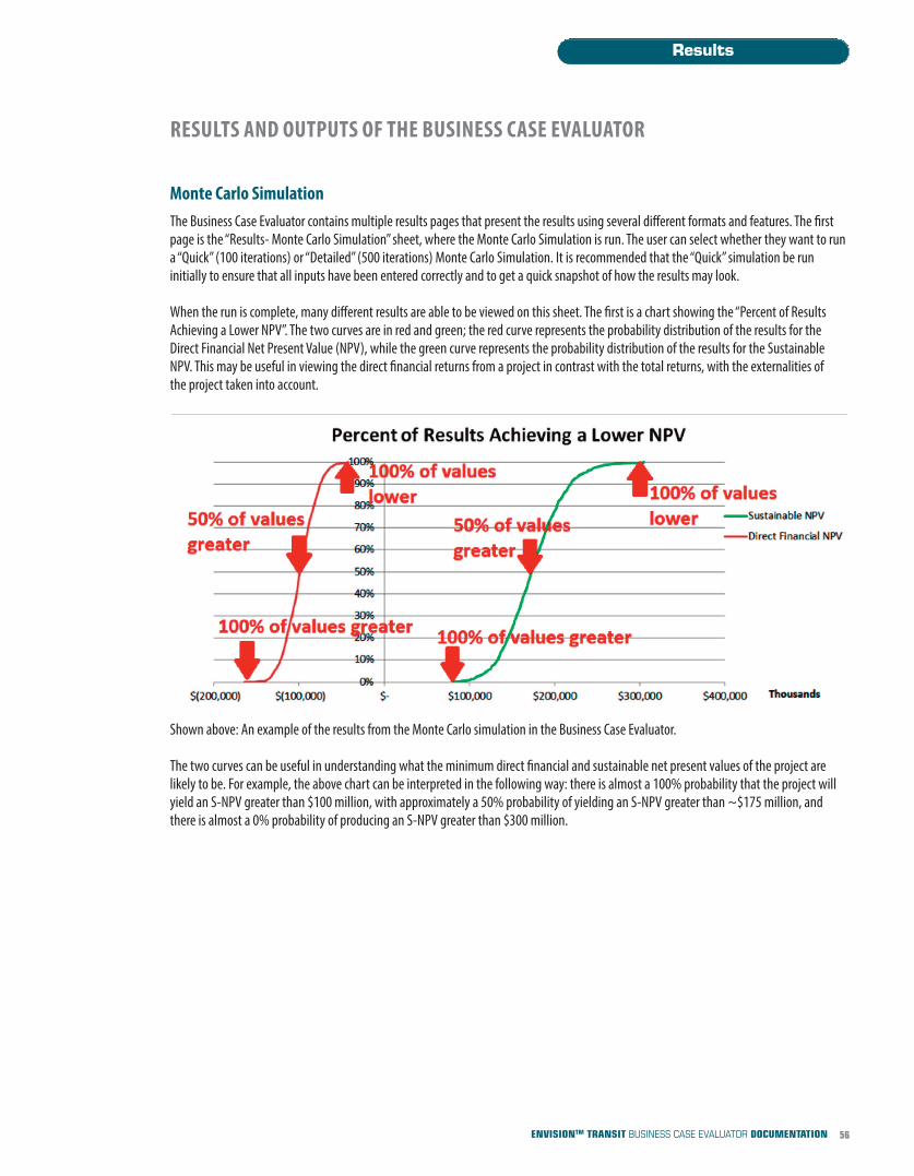
RESULTS AND OUTPUTS OF THE BUSINESS CASE EVALUATOR
Monte Carlo SimulationThe Business Case Evaluator contains multiple results pages that present the results using several different formats and features. The firstpage is the “Results- Monte Carlo Simulation” sheet, where the Monte Carlo Simulation is run. The user can select whether they want to runa “Quick” (100 iterations) or “Detailed” (500 iterations) Monte Carlo Simulation. It is recommended that the “Quick” simulation be run initially to ensure that all inputs have been entered correctly and to get a quick snapshot of how the results may look.
When the run is complete, many different results are able to be viewed on this sheet. The first is a chart showing the “Percent of ResultsAchieving a Lower NPV”. The two curves are in red and green; the red curve represents the probability distribution of the results for the Direct Financial Net Present Value (NPV), while the green curve represents the probability distribution of the results for the SustainableNPV. This may be useful in viewing the direct financial returns from a project in contrast with the total returns, with the externalities of the project taken into account.
Shown above: An example of the results from the Monte Carlo simulation in the Business Case Evaluator.
The two curves can be useful in understanding what the minimum direct financial and sustainable net present values of the project arelikely to be. For example, the above chart can be interpreted in the following way: there is almost a 100% probability that the project willyield an S-NPV greater than $100 million, with approximately a 50% probability of yielding an S-NPV greater than ~$175 million, andthere is almost a 0% probability of producing an S-NPV greater than $300 million.
Results
56ENVISIONTM TRANSIT BUSINESS CASE EVALUATOR DOCUMENTATION
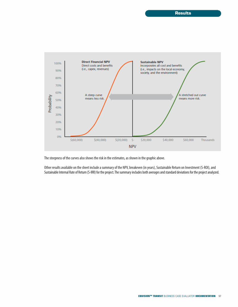
The steepness of the curves also shows the risk in the estimates, as shown in the graphic above.
Other results available on the sheet include a summary of the NPV, breakeven (in years), Sustainable Return on Investment (S-ROI), and Sustainable Internal Rate of Return (S-IRR) for the project. The summary includes both averages and standard deviations for the project analyzed.
Results
57ENVISIONTM TRANSIT BUSINESS CASE EVALUATOR DOCUMENTATION
Results SummaryThe results summary page contains charts and metrics so that the user can evaluate the value of the proposed project. The first charts thatcan be seen on the page are two pie charts, one showing a breakdown of the value from the benefits, and the second showing a breakdownof the value from the costs. These charts enable the user to view a quick visual representation of what most of the costs and benefits are attributed to.
Below the charts, there is a full breakdown of the results by “account”. These accounts include the following:
1. Direct financial value
2. Government or taxpayer
3. User/target-beneficiary or customer service
4. Economic or business activity
5. Environmental
6. Community or other
The methodology for how the values are allocated to each account can be found in the “Multiple Account Costs and Benefits” section of this document.
Similar to the multiple account breakdown, the results are also broken down by EnvisionTM Credit. Note that, unlike the stakeholder account breakdown that was shown above it, the sum of value attributed to the EnvisionTM credits do not necessarily add up to the total NPV of the project. This is because some of the costs and benefits are direct financial costs or benefits, hence they do not fit in any of the EnvisionTM credit buckets. The full methodology for how the values are allocated to each account can be found in the “Envision CreditCosts&Benefits” section of this document.
There are multiple metrics are provided to determine the financial viability of the proposed project. These include the profitability indices,discounted payback period, net present value, return on investment, internal rate of return, modified internal rate of return, and net present values of each individual cost or benefit.
Static ResultsThe static results page shows the median projected cash flows annually over the life of the project, broken down by each cost or benefit. The dates of project construction and project operation are taken into account, so that capital expenditure costs are paid when the project isunder construction, while operations costs and benefits are only counted when the project is in operation. Inflation is also taken into account in the calculations.
The values on the Static Results page are not “risk adjusted”. These values automatically use the most likely values (median or mid-point)values for each input in the model to create estimated projections over the life of the project.
Results
58ENVISIONTM TRANSIT BUSINESS CASE EVALUATOR DOCUMENTATION
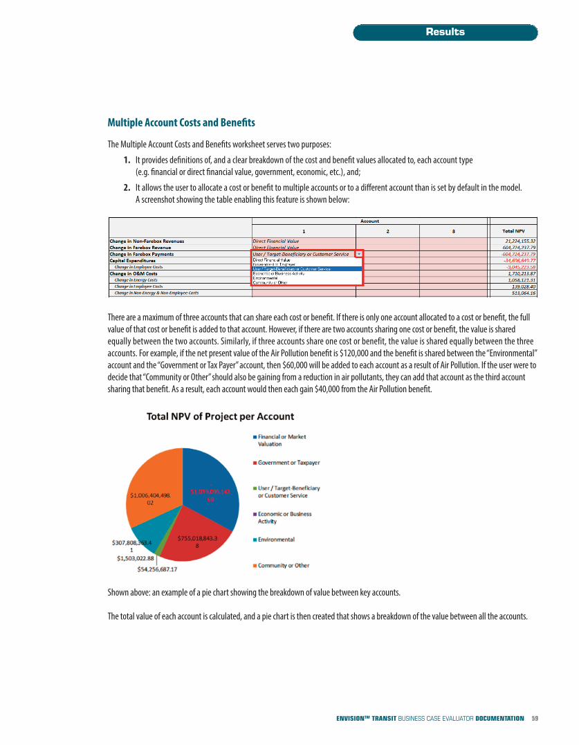
Results
59ENVISIONTM TRANSIT BUSINESS CASE EVALUATOR DOCUMENTATION
Multiple Account Costs and Benefits
The Multiple Account Costs and Benefits worksheet serves two purposes:
1. It provides definitions of, and a clear breakdown of the cost and benefit values allocated to, each account type (e.g. financial or direct financial value, government, economic, etc.), and;
2. It allows the user to allocate a cost or benefit to multiple accounts or to a different account than is set by default in the model. A screenshot showing the table enabling this feature is shown below:
There are a maximum of three accounts that can share each cost or benefit. If there is only one account allocated to a cost or benefit, the fullvalue of that cost or benefit is added to that account. However, if there are two accounts sharing one cost or benefit, the value is sharedequally between the two accounts. Similarly, if three accounts share one cost or benefit, the value is shared equally between the threeaccounts. For example, if the net present value of the Air Pollution benefit is $120,000 and the benefit is shared between the “Environmental”account and the “Government or Tax Payer” account, then $60,000 will be added to each account as a result of Air Pollution. If the user were todecide that “Community or Other” should also be gaining from a reduction in air pollutants, they can add that account as the third accountsharing that benefit. As a result, each account would then each gain $40,000 from the Air Pollution benefit.
Shown above: an example of a pie chart showing the breakdown of value between key accounts.
The total value of each account is calculated, and a pie chart is then created that shows a breakdown of the value between all the accounts.
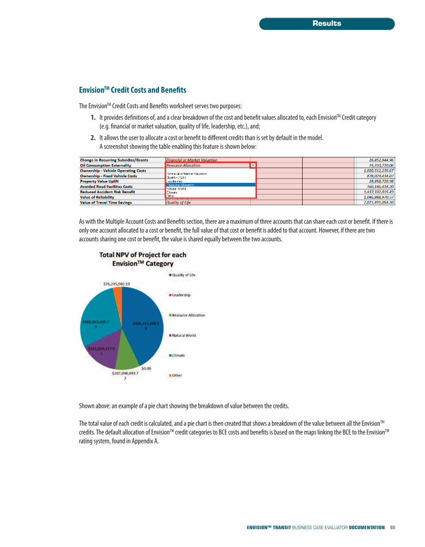
Results
60ENVISIONTM TRANSIT BUSINESS CASE EVALUATOR DOCUMENTATION
EnvisionTM Credit Costs and Benefits
The EnvisionTM Credit Costs and Benefits worksheet serves two purposes:
1. It provides definitions of, and a clear breakdown of the cost and benefit values allocated to, each EnvisionTM Credit category (e.g. financial or market valuation, quality of life, leadership, etc.), and;
2. It allows the user to allocate a cost or benefit to different credits than is set by default in the model. A screenshot showing the table enabling this feature is shown below:
As with the Multiple Account Costs and Benefits section, there are a maximum of three accounts that can share each cost or benefit. If there isonly one account allocated to a cost or benefit, the full value of that cost or benefit is added to that account. However, if there are two accounts sharing one cost or benefit, the value is shared equally between the two accounts.
Shown above: an example of a pie chart showing the breakdown of value between the credits.
The total value of each credit is calculated, and a pie chart is then created that shows a breakdown of the value between all the EnvisionTM
credits. The default allocation of EnvisionTM credit categories to BCE costs and benefits is based on the maps linking the BCE to the EnvisionTM
rating system, found in Appendix A.

Business Case EvaluatorAppendices
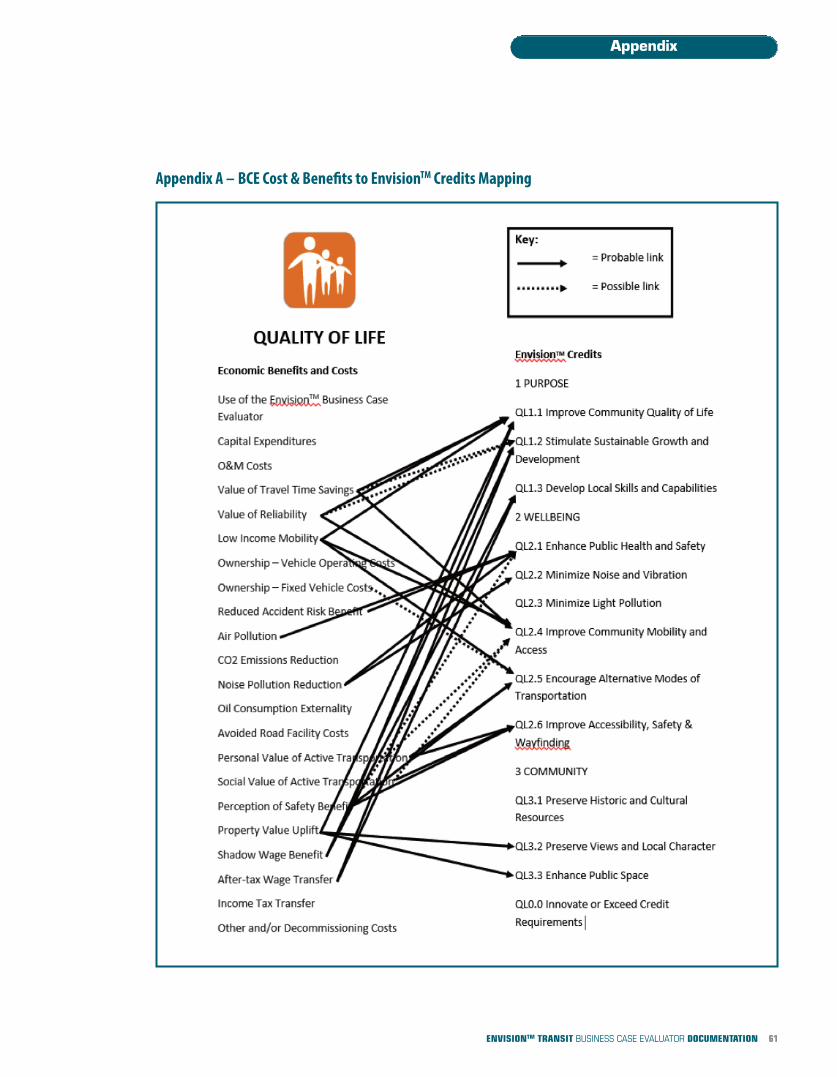
Appendix A – BCE Cost & Benefits to EnvisionTM Credits Mapping
Appendix
61ENVISIONTM TRANSIT BUSINESS CASE EVALUATOR DOCUMENTATION
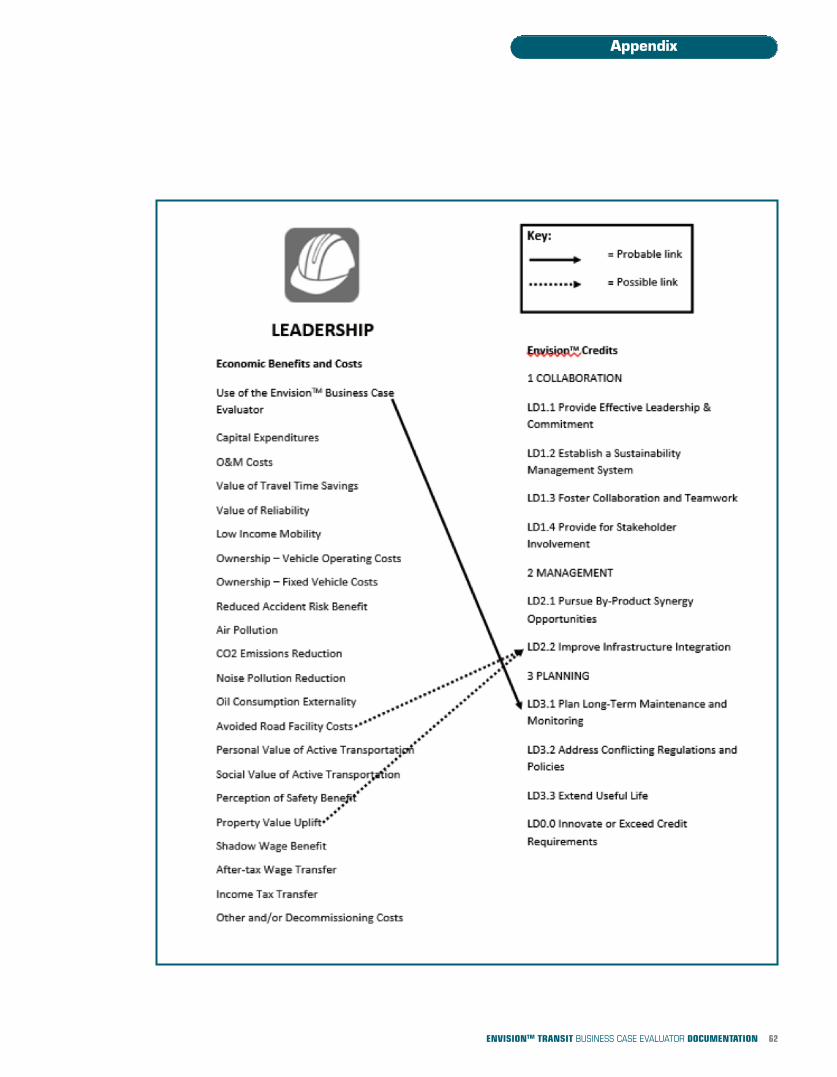
62ENVISIONTM TRANSIT BUSINESS CASE EVALUATOR DOCUMENTATION
Appendix
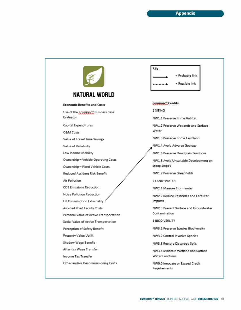
63ENVISIONTM TRANSIT BUSINESS CASE EVALUATOR DOCUMENTATION
Appendix
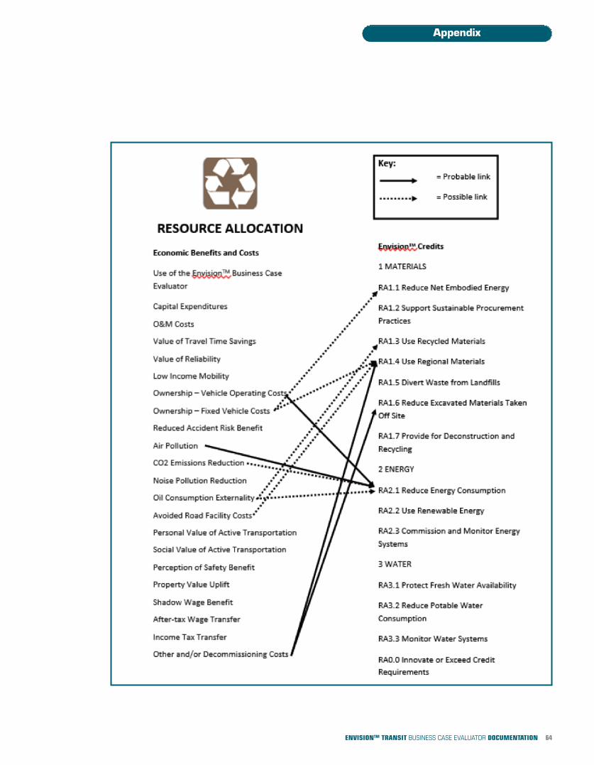
64ENVISIONTM TRANSIT BUSINESS CASE EVALUATOR DOCUMENTATION
Appendix
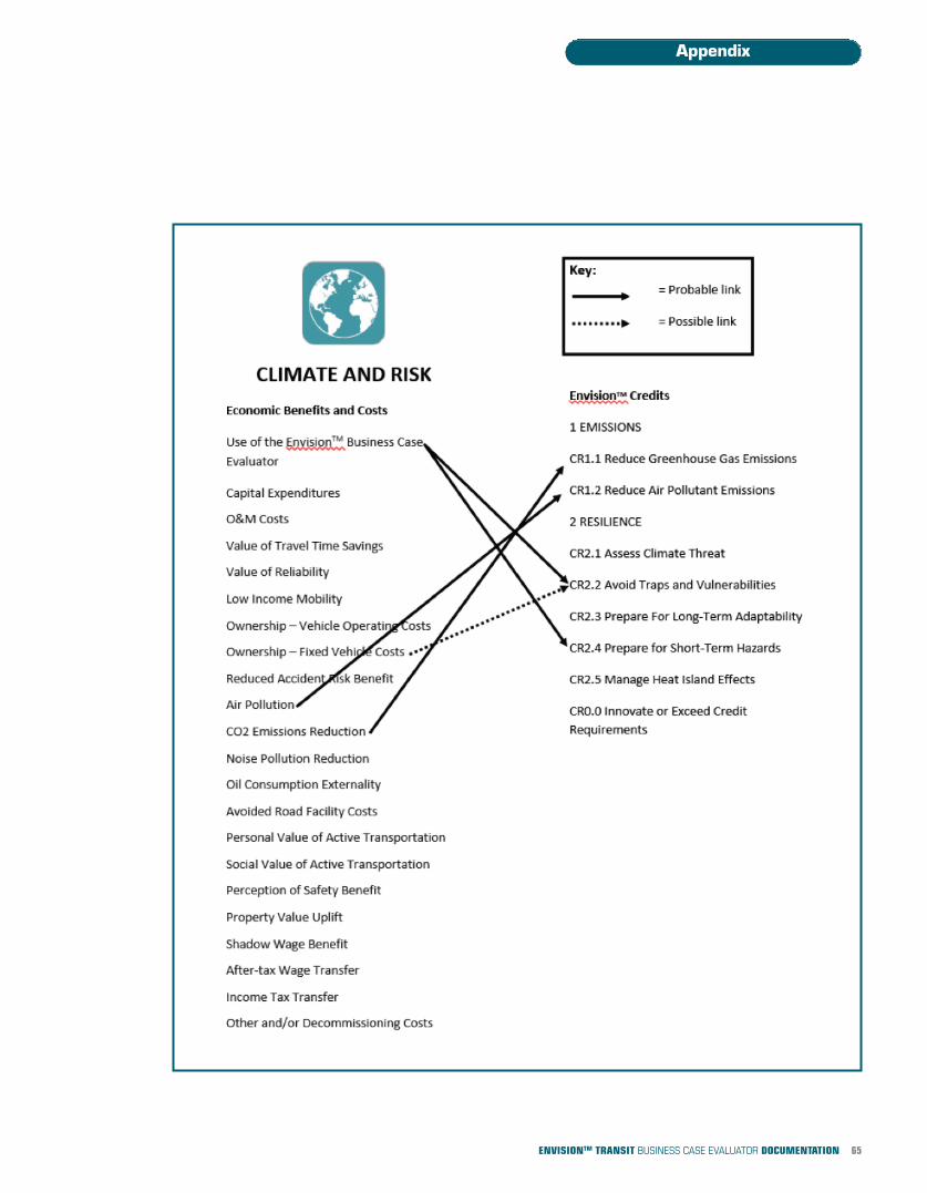
65ENVISIONTM TRANSIT BUSINESS CASE EVALUATOR DOCUMENTATION
Appendix
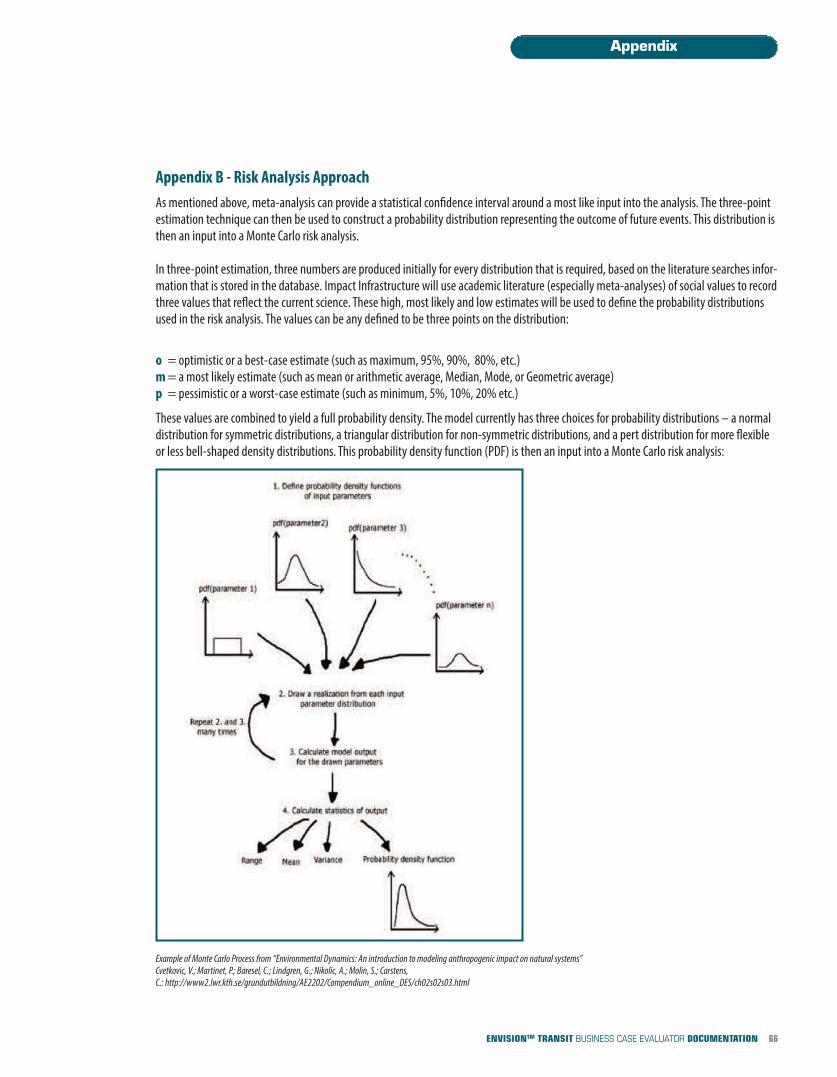
Appendix B - Risk Analysis ApproachAs mentioned above, meta-analysis can provide a statistical confidence interval around a most like input into the analysis. The three-pointestimation technique can then be used to construct a probability distribution representing the outcome of future events. This distribution isthen an input into a Monte Carlo risk analysis.
In three-point estimation, three numbers are produced initially for every distribution that is required, based on the literature searches infor-mation that is stored in the database. Impact Infrastructure will use academic literature (especially meta-analyses) of social values to recordthree values that reflect the current science. These high, most likely and low estimates will be used to define the probability distributionsused in the risk analysis. The values can be any defined to be three points on the distribution:
o = optimistic or a best-case estimate (such as maximum, 95%, 90%, 80%, etc.)m= a most likely estimate (such as mean or arithmetic average, Median, Mode, or Geometric average)p = pessimistic or a worst-case estimate (such as minimum, 5%, 10%, 20% etc.)
These values are combined to yield a full probability density. The model currently has three choices for probability distributions – a normaldistribution for symmetric distributions, a triangular distribution for non-symmetric distributions, and a pert distribution for more flexibleor less bell-shaped density distributions. This probability density function (PDF) is then an input into a Monte Carlo risk analysis:
Example of Monte Carlo Process from “Environmental Dynamics: An introduction to modeling anthropogenic impact on natural systems” Cvetkovic, V.; Martinet, P.; Baresel, C.; Lindgren, G.; Nikolic, A.; Molin, S.; Carstens, C.: http://www2.lwr.kth.se/grundutbildning/AE2202/Compendium_online_DES/ch02s02s03.html
66ENVISIONTM TRANSIT BUSINESS CASE EVALUATOR DOCUMENTATION
Appendix

For a trivial example of how the Monte Carlo analysis works, suppose the output is project return on investment (ROI) and it is calculated as return divided by investment. The return can be from -10 to +10 and the distribution is uniform (equal probability of each outcome betweenthese numbers). The investment can range from 90 (0.1% probability) to 110 (99.9% probability) with a most likely value of 100 (50% probability) and the values are given by a normal distribution. Assume the return and investment are independent of each other. Pick at randoma number between -10 and 10. Also pick a number at random from the normal distribution with mean 100 and standard deviation 3.3 (whichgives 90 at 0.1% level and 110 as 99.9% level). Calculate the ROI (return/investment) for this pair of random numbers and save the result (andinputs). Then repeat the process 100 times and graph the resulting ROI distribution and calculate summary statistics.
67ENVISIONTM TRANSIT BUSINESS CASE EVALUATOR DOCUMENTATION
Appendix
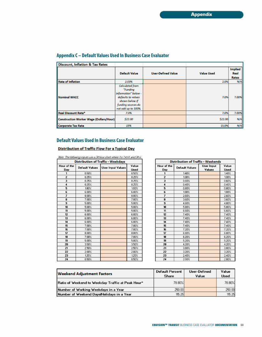
Appendix C – Default Values Used In Business Case Evaluator
Default Values Used In Business Case Evaluator
68ENVISIONTM TRANSIT BUSINESS CASE EVALUATOR DOCUMENTATION
Appendix
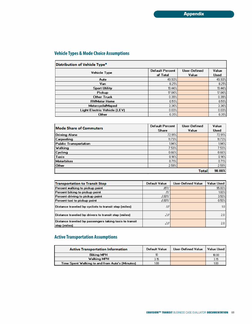
Vehicle Types & Mode Choice Assumptions
Active Transportation Assumptions
69ENVISIONTM TRANSIT BUSINESS CASE EVALUATOR DOCUMENTATION
Appendix
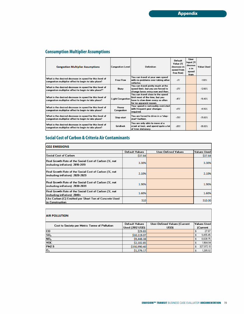
Consumption Multiplier Assumptions
Social Cost of Carbon & Criteria Air Contaminants
70ENVISIONTM TRANSIT BUSINESS CASE EVALUATOR DOCUMENTATION
Appendix
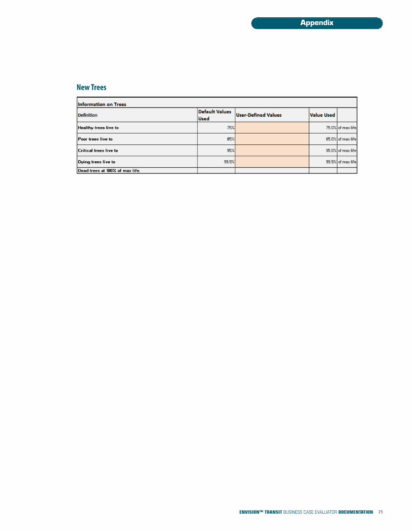
New Trees
71ENVISIONTM TRANSIT BUSINESS CASE EVALUATOR DOCUMENTATION
Appendix
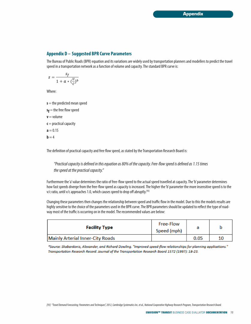
Appendix D – Suggested BPR Curve ParametersThe Bureau of Public Roads (BPR) equation and its variations are widely used by transportation planners and modellers to predict the travelspeed in a transportation network as a function of volume and capacity. The standard BPR curve is:
Where:
s= the predicted mean speed
sf= the free flow speed
v = volume
c= practical capacity
a= 0.15
b= 4
The definition of practical capacity and free flow speed, as stated by the Transportation Research Board is:
“Practical capacity is defined in this equation as 80% of the capacity. Free-flow speed is defined as 1.15 times the speed at the practical capacity.”
Furthermore the ‘a’ value determines the ratio of free-flow speed to the actual speed travelled at capacity. The ‘b’ parameter determineshow fast speeds diverge from the free-flow speed as capacity is increased. The higher the ‘b’ parameter the more insensitive speed is to thev/c ratio, until v/c approaches 1.0, which causes speed to drop off abruptly.[93]
Changing these parameters then changes the relationship between speed and traffic flow in the model. Due to this the models results arehighly sensitive to the choice of the parameters used in the BPR curve. The BPR parameters should be updated to reflect the type of road-way most of the traffic is occurring on in the model. The recommended values are below:
72ENVISIONTM TRANSIT BUSINESS CASE EVALUATOR DOCUMENTATION
Appendix
[93] “Travel Demand Forecasting: Parameters and Techniques”, 2012, Cambridge Systematics Inc. et al., National Cooperative Highway Research Program, Transportation Research Board.
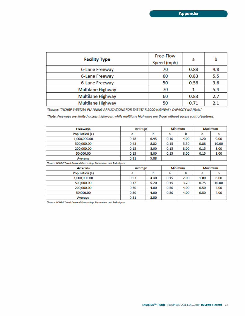
73ENVISIONTM TRANSIT BUSINESS CASE EVALUATOR DOCUMENTATION
Appendix
Appendix E – Social Discount RateThe social discount rate is used in the Sustainable Net Present Value (S-NPV) analysis.
The value of the social discount rate can have a large impact on the sustainable NPV of the scenarios. Lower discount rates will favor capitalintensive scenarios relative to those that have less capital upfront but perhaps more ongoing costs such as operating and maintenance(O&M) costs. As an example a 3% discount rate applied to a $100 cost 100 years from now is equivalent to about $5 today. At an 8% dis-count rate the cost would be only about $0.05 in present day terms.
The social discount rate can be thought of as measuring a time preference for the present over the future and an opportunity cost that usingresources today means that they are not invested for use later. The time preference can also be thought of as being composed of a pure timepreference and a premium for the uncertainty that benefits and costs in future will materialize.
Alternatively, the social discount rate can be thought of as measuring the opportunity for re-investment and compounding of benefits re-ceived or costs deferred.
These three effects are called, in the economics literature, the rate of time preference, the risk adjustment of the discount rate, and the so-cial opportunity cost of capital.
For U.S. government analyses the OMB recommends using both the time preference rate (which tends to be lower and is estimated at 3 %in real terms on a pre-tax basis) and the opportunity cost rate (which is higher and estimated at a real pre-tax 7% rate, reflecting the fore-gone rate of return). For Canadian government analyses the Canadian Federal Government recommends using a real rate of 8%.
Social Opportunity Cost of Capital
The social opportunity cost of capital is the expected rate of return forgone from other potential investments. “If government investmentcomes at the expense of private investment, the cost to the economy is measured by the social returns that would have been generated bythat investment. This has been variously labelled the investment rate of interest, the producer rate of interest, the marginal rate of return toinvestment or capital, the marginal efficiency or product of capital, or the social opportunity cost of capital.”[94]
The U.S. federal government Office of Management and Budget (OMB) estimated[95] that social opportunity cost of capital as measured bythe real, pre-tax rate[96] of return on all sources of private capital in the United States is approximately 7%. This rate is the social opportunitycost of capital it is the cost of diverting funds to government projects that could be productively used elsewhere; “it is the appropriate dis-count rate whenever the main effect of a regulation is to displace or alter the use of capital in the private sector.” [97]
The OMB also notes that if a project is expected to displace corporate business investment then sensitivity at a higher than 7% rate also bedone, reflecting the foregone rate of return. If business investment alone is used as a source of capital the OMB puts this figure at about10%. In addition, the recommended 7% social opportunity cost of capital only reflects the average degree of risk of displaced projects itdoes not include any premium of adjustment for the uncertainty of degree of uncertainty of risk for the scenarios considered.
74ENVISIONTM TRANSIT BUSINESS CASE EVALUATOR DOCUMENTATION
Appendix
[94] Valuing the Future: the social discount rate in cost-benefit analysis by Mark Harrison for the Australian Productivity Commission. April 2010[95] Circular A-4 http://www.whitehouse.gov/omb/circulars_a004_a-4, Circular A-94 Guidelines And Discount Rates For Benefit-Cost Analysis of Federal[96] The OMB states that “The pre-tax rates of return better measure society's gains from investment “because of the distortions due to taxes. Economic distortions, including taxes on capital,
create a divergence between the rate of return that savers earn and the private rate of return to capital. This divergence persists despite the tendency for capital to flow to where it can earn the highest rate of return. Although market forces will push after-tax rates of return in different sectors of the economy toward equality, that process will not equate pre-tax rates of return when there are differences in the tax treatment of investment. Corporate capital, in particular, pays an additional layer of taxation, the corporate income tax, which requires it to earn a higher pre-tax rate of return in order to provide investors with similar after-tax rates of return compared with non-corporate investments.”
[97] OMB Circular A-4 http://www.whitehouse.gov/omb/circulars_a004_a-4
75ENVISIONTM TRANSIT BUSINESS CASE EVALUATOR DOCUMENTATION
Appendix
Rate of Time Preference“We saw why individuals might have a pure time rate of preference: People are impatient; they don't live forever; possessions can be lost,destroyed, or stolen, and opportunities disappear. A reasonable individual may discount the future for any one of these reasons-why shouldI pay money now to reduce damages from global warming that will only occur after I am dead?-but the same logic does not apply to soci-ety: Relative to the individuals of which they are composed, societies are immortal and uncertainties are averaged out. For this reason,there is, in fact, fairly wide consensus within the economics profession that social discount rates should indeed be lower than individual dis-count rates. The social discount rate is a rate of conversion of future value to present value that reflects society's collective ethical judgment,as opposed to an individualistic judgment, such as the market rate of interest.”[98]
“When regulation primarily and directly affects private consumption (e.g., through higher consumer prices for goods and services), a lowerdiscount rate is appropriate. The alternative most often used is sometimes called the "social rate of time preference." This simply means therate at which "society" discounts future consumption flows to their present value. If we take the rate that the average saver uses to discountfuture consumption as our measure of the social rate of time preference, then the real rate of return on long-term government debt mayprovide a fair approximation. Over the last thirty years, this rate has averaged around 3 percent in real terms on a pre-tax basis. For exam-ple, the yield on 10-year Treasury notes has averaged 8.1 percent since 1973 while the average annual rate of change in the CPI over thisperiod has been 5.0 percent, implying a real 10-year rate of 3.1 percent.”
So, the OMB estimates the time preference rate at 3.1% and the social opportunity cost of capital to be 7%. U.S. government guidelinessuggest that both be used, a base rate of 7% and a sensitivity of 3.1%.
Social Discount Rate and Sustainability
The social rate of discount is a contentious issue. For sustainability analysis in particular, there is much dissension because of the long-timehorizons involved. Some sustainability advocates have argued for a zero or very low discount rate so that long-lived environmental costs aredealt with sooner rather than deferred for future generations. Or alternatively, the benefits of distantly realized environmental improve-ments are not reduced in decision made today. A zero discount rate gives equal weight to present and future generations.
[98] Ecological Economics: Principles and Applications, Herman Daly and Joshua Farley, Washington: Island Press, 2004, pp.273-274.
76ENVISIONTM TRANSIT BUSINESS CASE EVALUATOR DOCUMENTATION
Appendix
From the U.S. EPA:
"Analysts disagree whether long time horizon problems merit special consideration. Some economists and policy analysts argue that bene-fits accruing to future generations should not be discounted at all. Others believe that intergenerational concerns can often be addressed byusing a social rate of time preference—the rate of time preference modified to reflect intergenerational equity considerations …The draftEPA white paper on discounting suggests that when faced with a situation involving intergenerational concerns, the analyst should ac-knowledge that both sides of this debate have merit and calculate the present value of future benefit streams using both a zero discountrate (not discounting at all) and the rate of time preference (effectively discounting all expected future benefits in the same way)…"[99]
One argument for a low rate when considering sustainability issues is that the opportunity cost of capital depends on growth and sustain-ability advocates point out “the economy as a whole cannot grow indefinitely, in which case a social discount rate into the indefinite futuremay be inappropriate.”[100]
Also, the profitability of investments used in the opportunity cost calculation “are ‘profitable’ because we ignore many of the costs of pro-duction. We know that all human productive activities use up natural resources and return waste to the environment, and these costs ofproduction are often ignored.” [101]
“Applying a zero discount rate also presumes that the estimates of very long-term consequences are as reliable as estimates of conse-quences that are expected in the short term. It gives equal weight to an estimated consequence in hundreds of years as it does to one thatwill occur today, even though there is much less reason to believe that the future consequence will unfurl as currently predicted …There islittle doubt that people value sustainability and are concerned about the state of the environment and the quality of life that future genera-tions will inherit. However there are better ways to take this into account in benefit-cost analysis than by imposing a zero discount rate inthe evaluation of forecast long-term consequences.” [102]
The OMB recommends that if a project “will have important intergenerational benefits or costs you might consider a further sensitivityanalysis using a lower but positive discount rate in addition to calculating net benefits using discount rates of 3 and 7 percent.” (Emphasis added).
U.S. Department of Transportation (USDOT) Transportation Investment Generating Economic Recovery (TIGER) Discretionary Grants guid-ance recommends the same (7% or 3%) discount rate but also a 3% for monetized carbon dioxide emissions benefits and costs (Social Costof Carbon or SCC): “…carbon emissions are valued differently from other benefits and costs from the perspective of discount rate. Appli-cants should continue to calculate discounted present values for all benefits and costs (that exclude carbon dioxide emissions) at 7% and3%, as recommended by OMB Circular A-94. To these non-carbon NPV benefits, the Applicant should then add the corresponding net valueof carbon dioxide emissions, as calculated from the 3% SCC value.” [104]
[99] U.S. Environmental Protection Agency Office of Air Quality Planning and Standards Innovative Strategies and Economics Group “OAQPS Economic Analysis Resource Document”http://www.epa.gov/ttnecas1/econdata/Rmanual2/8.3.html
[100] Ecological Economics: Principles and Applications, Herman Daly and Joshua Farley, Washington: Island Press, 2004, pp.273-274.[101] Ibid.[102] Multiple Account Benefit-Cost Analysis A Practical Guide for Systematic Evaluation of Project and Policy Alternatives by Marvin Shaffer, University of Toronto Press, 2010, pp. 130-1[103] OMB Circular A-4 Op. Cit.[104] TIGER BCA Resource Guide(2014) http://www.dot.gov/sites/dot.gov/files/docs/TIGER%20BCA%20Resource%20Guide%202014.pdf
77ENVISIONTM TRANSIT BUSINESS CASE EVALUATOR DOCUMENTATION
Appendix
International ComparisonsSocial discount rate recommendations vary considerably. One review across countries identifies recommendations ranging from 1 to 15%.[105]
In small open economies, such as Canada, calculations of a weighted average social opportunity cost of capital depends on how much pri-vate investment is displaced and the ability to attract foreign investment. The lower limit on the estimate should be the cost of foreign bor-rowing. Federal government estimates of real pre-tax rates in Canada have fallen from 10% to 8% but have always been higher than theU.S. 7% rate. In a contrary view, for the province of Ontario, Spiro[106] estimates the social discount to be a real 5% rate of return.
Social Discount Rate Conclusion
The BCE follows the U.S. Federal Government guidance and uses a 7% real discount rate as the default rate for U.S. projects. When availablein the BCE for Transit, for Canadian projects the BCE will follow the Canadian Federal Government guidance and use an 8% real discount rateas the default rate. These recommended values can be over-ridden in the advanced inputs section.
The BCE also gives the user the option to use a private discount rate or Weighted Average Cost of Capital (WACC) instead of the social cost ofcapital. If the project proponent is a private entity this may be appropriate. The private discount rate or weighted average cost of capital canbe input using the funding sources and costs or the overall resulting WACC.
[105] Valuing the Future: the social discount rate in cost-benefit analysis. Visiting Research Paper, April 2010. Australian Government. Productivity Commission. Mark Harrison 2010[106] The Social Discount Rate for Provincial Government Investment Projects by Peter S. Spiro http://www.peterspiro.com/Social_Discount_Rate.pdf
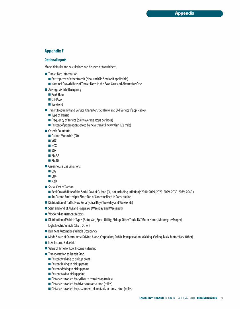
78ENVISIONTM TRANSIT BUSINESS CASE EVALUATOR DOCUMENTATION
Appendix
Appendix F
Optional Inputs
Model defaults and calculations can be used or overridden:
n Transit Fare Informationn Per-trip cost of other transit (New and Old Service if applicable)nNominal Growth Rate of Transit Fares in the Base Case and Alternative Case
n Average Vehicle Occupancy n Peak Hourn Off-PeaknWeekend
n Transit Frequency and Service Characteristics (New and Old Service if applicable)n Type of Transitn Frequency of service (daily average stops per hour)n Percent of population served by new transit line (within 1/2 mile)
n Criteria Pollutantsn Carbon Monoxide (CO)n VOCnNOXn SOXn PM2.5n PM10
n Greenhouse Gas Emissionsn CO2n CH4nN2O
n Social Cost of Carbonn Real Growth Rate of the Social Cost of Carbon (%, not including inflation): 2010-2019, 2020-2029, 2030-2039, 2040+n lbs Carbon Emitted per Short Ton of Concrete Used in Construction
n Distribution of Traffic Flow For a Typical Day (Weekday and Weekends)n Start and end of AM and PM peaks (Weekday and Weekends)n Weekend adjustment factorsn Distribution of Vehicle Types (Auto, Van, Sport Utility, Pickup, Other Truck, RV/Motor Home, Motorcycle/Moped,
Light Electric Vehicle (LEV), Other)n Business Automobile Vehicle Occupancyn Mode Share of Commuters (Driving Alone, Carpooling, Public Transportation, Walking, Cycling, Taxis, Motorbikes, Other)n Low Income Ridershipn Value of Time for Low Income Ridershipn Transportation to Transit Stopn Percent walking to pickup pointn Percent biking to pickup pointn Percent driving to pickup pointn Percent taxi to pickup pointn Distance travelled by cyclists to transit stop (miles)n Distance travelled by drivers to transit stop (miles)n Distance travelled by passengers taking taxis to transit stop (miles)
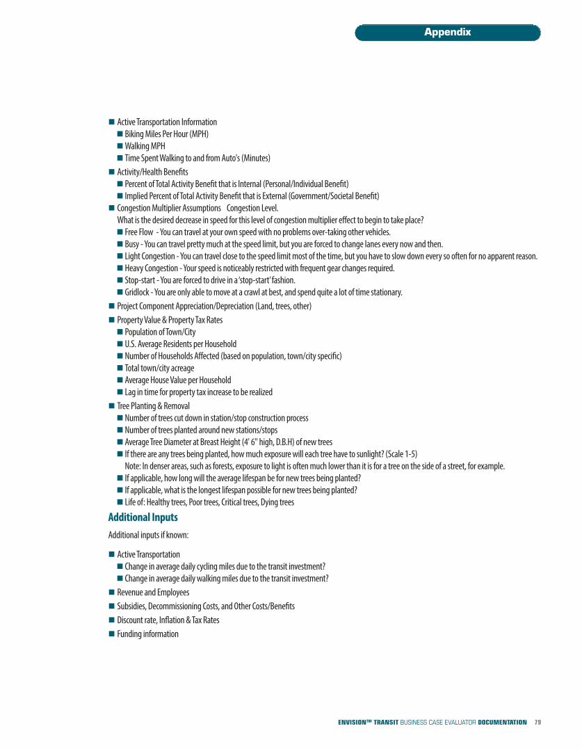
79ENVISIONTM TRANSIT BUSINESS CASE EVALUATOR DOCUMENTATION
Appendix
n Active Transportation Informationn Biking Miles Per Hour (MPH)nWalking MPHn Time Spent Walking to and from Auto's (Minutes)
n Activity/Health Benefitsn Percent of Total Activity Benefit that is Internal (Personal/Individual Benefit)n Implied Percent of Total Activity Benefit that is External (Government/Societal Benefit)
n Congestion Multiplier Assumptions Congestion Level. What is the desired decrease in speed for this level of congestion multiplier effect to begin to take place?n Free Flow - You can travel at your own speed with no problems over-taking other vehicles.n Busy - You can travel pretty much at the speed limit, but you are forced to change lanes every now and then.n Light Congestion - You can travel close to the speed limit most of the time, but you have to slow down every so often for no apparent reason.n Heavy Congestion - Your speed is noticeably restricted with frequent gear changes required.n Stop-start - You are forced to drive in a ‘stop-start’ fashion.n Gridlock - You are only able to move at a crawl at best, and spend quite a lot of time stationary.
n Project Component Appreciation/Depreciation (Land, trees, other)n Property Value & Property Tax Ratesn Population of Town/Cityn U.S. Average Residents per HouseholdnNumber of Households Affected (based on population, town/city specific)n Total town/city acreagen Average House Value per Householdn Lag in time for property tax increase to be realized
n Tree Planting & RemovalnNumber of trees cut down in station/stop construction processnNumber of trees planted around new stations/stopsn Average Tree Diameter at Breast Height (4' 6" high, D.B.H) of new treesn If there are any trees being planted, how much exposure will each tree have to sunlight? (Scale 1-5)
Note: In denser areas, such as forests, exposure to light is often much lower than it is for a tree on the side of a street, for example.n If applicable, how long will the average lifespan be for new trees being planted? n If applicable, what is the longest lifespan possible for new trees being planted?n Life of: Healthy trees, Poor trees, Critical trees, Dying trees
Additional Inputs Additional inputs if known:
n Active Transportationn Change in average daily cycling miles due to the transit investment?n Change in average daily walking miles due to the transit investment?
n Revenue and Employeesn Subsidies, Decommissioning Costs, and Other Costs/Benefitsn Discount rate, Inflation & Tax Ratesn Funding information

Business Case EvaluatorReferences
REFERENCES
General:Marvin Shaffer, (2010), “Multiple Account Benefit-Cost Analysis: A Practical Guide for the Systematic Evaluation of Project and Policy Alternatives”,University of Toronto Press.
The Value of Travel Time Savings:Bureau of Transport and Regional Economics, (2006), “National Guidelines for Transport System Management in Australia”, Australian TransportCouncil, http://www.transportinfrastructurecouncil.gov.au/publications/files/National_Guidelines_Volume_3.pdf.Congressional Budget Office, (2013), “The Long-Term Outlook for the Federal Budget”, http://www.cbo.gov/sites/default/files/44521-LTBO2013_0.pdf.
Gary Becker, (1965), “A theory of the allocation of time”, The Economic Journal 75, 493-517,http://econ.tu.ac.th/class/archan/SUPACHAI/EE471/Chapter%202/Chapter2_A%20Theory%20of%20the%20Allocation%20of%20Time.pdf.
P.J. Mackie et al., (2001), “The value of travel time savings in evaluation”, Transportation Research Part E,http://www.sciencedirect.com/science/article/pii/S1366554500000132.
Roberto Ayala, (2014), “The Value of Travel Time Savings: Departmental Guidance for Conduction Economic Evaluations Revision 2 (2014 Update)”,United States Department of Transportation.
Sergio Jara-Diaz, (1999), “On the Subjective Valuation of Travel Time Savings”, PTRC Education and Research Services, Transportation PlanningMethods: Proceedings of Seminar F, http://www.worldcat.org/title/transportation-planning-methods-proceedings-of-seminar-f-held-at-the-eu-ropean-transport-conference-robinson-college-cambridge-27-29-september-1999/oclc/43034916.
Sergio Jara-Diaz, (2002), “The Goods/ Activities Framework for Discrete Travel Choices: Indirect Utility and Value of Time”, In Perpetual Motion:Travel Behavior Research Opportunities and Challenges, http://www.cec.uchile.cl/~dicidet/sjara/GoodsActivitiesFrameork.PDF.
Sisinnio Concas, et al., (2009), “Synthesis of Research on Value of Time and Value of Reliability”, Florida Department of Transportation,http://www.nctr.usf.edu/pdf/77806.pdf.
Todd Litman, (2012), “Transportation Cost and Benefit Analysis II – Travel Time Costs”, Victoria Transport Policy Institute,http://www.vtpi.org/tca/tca0502.pdf.
The Value of Congestion:
Mark Wardman and J. Nicolas Ibanez, (2012), “The congestion multiplier: Variations in motorists’ valuation of travel time with traffic conditions”,Transportation Research Part A,http://www.researchgate.net/publication/257424718_The_congestion_multiplier_Variations_in_motorists_valuations_of_travel_time_with_traffic_conditions.
New Zealand Transport Agency, (2013), “Economic evaluation manual”, http://www.nzta.govt.nz/resources/economic-evaluation-manual/eco-nomic-evaluation-manual/eem.html.
Pedro Abrantes and Mark Wardman, (2009), “Meta-Analysis of UK Values of Time: An Update”, Institute for Transport Studies, Transportation Re-search Part A, http://www.sciencedirect.com/science/article/pii/S0965856410001242.
Steer Davies Gleave, (2004), “Effect of Road Congestion on Rail Demand: Technical Report“, Prepared for Passenger Demand Forecasting Council,Association of Train Operating Companies, London.
continued
References
80ENVISIONTM TRANSIT BUSINESS CASE EVALUATOR DOCUMENTATION
The Value of ReliabilityAbdel-Aty, M., Kitamura, R. and Jovanis, P. (1995), “Investigating effects of travel time variability on route choice using repeated-measurementstated preference data”, Transportation Research, 1493, pp. 39-45.
Asensio, J., Matas, A., (2008), “Commuters’ valuation of travel time variability”, Transportation Research Part E: Logistics and Transportation Review44, 1074–1085.
Bates, J., Polak, J., Jones, P., and Cook A. (2001), “The valuation of reliability for personal travel”, Transportation Research Part E (Logistics and Trans-portation Review), 37-2/3, pp. 191-229.
Bhat, C., Sardesai, R., (2006), “The impact of stop-making and travel time reliability on commute mode choice”, Transportation Research Part B:Methodological 40, 709–730.
Black, I., Towriss, J., (1993), “Demand effects of travel time reliability. Technical Report”, Centre for Logistics and Transportation, Craneld Institute ofTechnology.
Brownstone, K. and Small, K. (2002), “Valuing time and reliability: assessing evidence from road pricing demonstrations”, University of California,Irvine.
Bureau of Transport and Regional Economics, (2006), “National Guidelines for Transport System Management in Australia”, Australian TransportCouncil, http://www.transportinfrastructurecouncil.gov.au/publications/files/National_Guidelines_Volume_3.pdf.
Cambridge Systematics, Inc., (2013), “Analytical Procedures for Determining the Impacts of Reliability Mitigation Strategies”, Strategic Highway Re-search Program, Transportation Research Board.
Carrion, C., Levinson, D., (2010), “Value of reliability: high occupancy toll lanes, general purpose lanes, and arterials”, Conference Proceedings of 4thInternational Symposium on Transportation Network Reliability in Minneapolis, MN (USA).
Carrion, C., Levinson, D., (2011), “A model of bridge choice across the Mississippi river in Minneapolis”, Levinson, D., Liu, H., Bell, M. (Eds.), NetworkReliability in Practice: Selected Papers from the Fourth International Symposium on Transportation Network Reliability. Springer, pp. 115–129,chapter 8.
Carrion, C., Levinson, D., (2012), “Value of travel time reliability: A review of current evidence”, Transportation Research Part A, Department of CivilEngineering, University Minnesota.
De Jong, G., Tseng, Y., Kouwenhoven, M., Verhoef, E., Bates, J., (2007), “The value of travel time and travel time reliability. Technical report”, TheNetherlands Ministry of Transport, Public Works and Water Management.
DfT, (2009), “The Reliability Sub-Objective, TAG Unit 3.5.7.”, United Kingdom Department for Transport,www.dft.gov.uk/webtag/webdocuments/3_Expert/5_Economy_Objective/3.5.7.htm.
Eliasson, J. (2004), “Car drivers’ valuations of travel time variability, unexpected delays and queue driving”, Proceedings of the European TransportConference, 2004.
Ghosh, A., (2001), “Valuing time and reliability: commuters’ mode choice from a real time congestion pricing experiment. PhD thesis”, University ofCalifornia, Irvine (USA).
Hamer, R., De Jong, G. and Kroes, E. (2005), “The value of reliability in Transport – Provisional values for the Netherlands based on expert opinion”,RAND Technical Report Series, TR-240-AVV, Netherlands.
continued
81ENVISIONTM TRANSIT BUSINESS CASE EVALUATOR DOCUMENTATION
References
Hollander, Y., (2006), “Direct versus indirect models for the effects of unreliability”, Transportation Research Part A: Policy and Practice 40, 699–711.
Jonas Eliasson, (2006), “Forecasting Travel Time Variability”, Transek AB, Association for European Transport.Koskenoja, P., (1996). “The Effect of Unreliable Commuting Time on Commuter Preferences. PhD thesis”, University of California, Irvine (USA).
Li, Z., Tirachini, A., Hensher, D., (2010), “Embedding risk attitudes in a scheduling model: application to the study of commuting departure time”,Conference Proceedings of 4th International Symposium on Transportation Network Reliability in Minneapolis, MN (USA).
Liu, H., He, X., Recker, W., (2007), “Estimation of the time-dependency of values of travel time and its reliability from loop detector data”, Trans-portation Research Part B: Methodological 41, 448–461.
Liu, H., Recker, W., Chen, A., (2004), “Uncovering the contribution of travel time reliability to dynamic route choice using real-time loop data”, Trans-portation Research Part A 38, 435–453.
Mogens Fosgerau and Anders Karlstrom, (2007), “The Value of reliability”, Munich Personal RePEc Archive, http://mpra.ub.uni-muenchen.de/5733/1/MPRA_paper_5733.pdf
Mogens Fosgerau, (2010), “What is the value of reliability”, Centre for Transport Studies Stockholm.
Mogens Fosgerau, Katrine Hjorth, Cmilla Brems, Daisuke Fukuda, (2008), “Travel time variability Definition and valuation”, Danish Ministryof Transportation.
New Zealand Transport Agency, (2008), “Economic Evaluation Manual, Volume 1, Amendment No 2, September 2008”, New Zealand TransportAgency. www.nzta.govt.nz.
New Zealand Transport Agency, (2013), “Economic Evaluation Manual”, New Zealand Transport Agency, http://www.nzta.govt.nz/resources/eco-nomic-evaluation-manual/economic-evaluation-manual/eem.html.
Sisinnio Concas, et al., (2009), “Synthesis of Research on Value of Time and Value of Reliability”, Florida Department of Transportation,http://www.nctr.usf.edu/pdf/77806.pdf.
Small, K, Noland, R., Chu, X. and Lewis, D. (1999), “Valuation of travel time savings and predictability in congested conditions for highway user-costestimation”, Report 431, National Cooperative Highway Research Program, Washington, D.C.
Small, K., Noland, R., Chu, X., Lewis, D., (1999), “Valuation of travel-time savings and predictability in congested conditions for highway user-costestimation. Technical report”, National Cooperative Highway Research Program Report 431.
Small, K., Noland, R., Koskenoja, P., (1995), “Socio-economic attributes and impacts of travel reliability: a stated preference approach. Technical re-port”, California PATH Research Report, UCB-ITS-PRR-95-36.
Small, K., Winston, C., Yan, J., (2005), “Uncovering the distribution of motorists’ preferences for travel time and reliability”, Econometrica 73,1367–1382.
Stefanie Peer, Carl Koopmans, Erik Verhoef, (2009), “Predicting Travel Time Variability for Cost-Benefit-Analysis”, Department for Spatial EconomicsVU University.
Tilahun, N., Levinson, D., (2010), “A moment of time: reliability in route choice using stated preference”, Journal of Intelligent Transportation Sys-tems 14, 179–187.
Transport Research Centre, (2010), “Improving Reliability on Surface Transport Networks”, International Transport Forum, OECD.
Transport Research Centre, (2010), “Improving Reliability on Surface Transport Networks”, International Transport Forum, OECD.
Yan, J., (2002), “Heterogeneity in motorists’ preferences for travel time and time reliability: empirical finding from multiple survey data sets and itspolicy implications. PhD thesis”, University of California, Irvine(USA).http://www.dot.gov/sites/dot.gov/files/docs/TIGER%20BCA%20Resource%20Guide%202014.pdf.
continued
References
82ENVISIONTM TRANSIT BUSINESS CASE EVALUATOR DOCUMENTATION
Low Income Mobility Benefit:Colliers International, (2012), “2012 Parking Survey”, http://www.collierscanada.com/en/news/2012/parking%20survey%202012#.VXsGFEaz-mAU.
David Lewis, Fred Laurence Williams, (1999), “Policy and Planning as Public Choice: Mass Transit in the United States”, United States Department ofTransportation, http://www.fta.dot.gov/documents/Policy_and_Planning_as_Public_Choice.pdf.
John Parker, (2008), “Costs of Road Congestion in the Greater Toronto and Hamilton Area: Impact and Cost Benefit Analysis of the Metrolinx DraftRegional Transportation Plan”, HDR Corporation Decision Economics, Greater Toronto Transportation Authority, Risk Analysis Investment and Fi-nance Economics and Policy, http://www.metrolinx.com/en/regionalplanning/costsofcongestion/ISP_08-015_Cost_of_Congestion_report_1128081.pdf.
Misty L. Heggeness, Charles Hokayem, (2012), “Life on the Edge: Living Near Poverty in the United States, 1966-2011”, SEHSD Working Paper 2013-02, http://www.census.gov/hhes/www/poverty/publications/WP2013-02.pdf.
Taxi Fare Finder, (2015), “Rate Chart”, retrieved from http://www.taxifarefinder.com/rates.php.
United States Census Bureau, (2013), “American Community Survey 5-Year Average, All US Metro and Micropolitan Areas”, retrieved fromhttp://factfinder.census.gov/faces/nav/jsf/pages/index.xhtml.
Ownership – Operating Costs:American Automobile Association, (2013), “Your Driving Costs: How much are you really paying to drive?”, http://exchange.aaa.com/wp-content/uploads/2013/04/Your-Driving-Costs-2013.pdf.
Insurance Institute for Highway Safety Highway Loss Data Institute, (2013), “Fatality Facts”, http://www.iihs.org/iihs/topics/t/general-statistics/fa-talityfacts/passenger-vehicles.
Todd Litman, (2012), “Transportation Cost and Benefit Analysis II – Noise Costs”, Victoria Transport Policy Institute,http://www.vtpi.org/tca/tca0504.pdf.
Ownership – Fixed Costs:John Holtzclaw, Robert Clear, Hank Dittmar, David Goldstein , (2002), “Location Efficiency: Neighborhood and Socio-Economic Characteristics De-termine Auto Ownership and Use – Studies in Chicago, Los Angeles and San Fransisco”, Transportation Planning and Technology,http://www.tandfonline.com/doi/abs/10.1080/03081060290032033.
ECONorthwest and Parsons Brinckerhoff Quade & Douglas, Inc., (2002), “Estimating the Benefits and Costs of Public Transit Projects: A Guidebookfor Practitioners”, Transit Cooperative Research Program, Federal Transit Administration.http://www.tcrponline.org/PDFDocuments/tcrp_rpt_78.pdf.
American Automobile Association, (2013), “Your Driving Costs: How much are you really paying to drive?”, http://exchange.aaa.com/wp-content/uploads/2013/04/Your-Driving-Costs-2013.pdf.
Insurance Institute for Highway Safety Highway Loss Data Institute, (2013), “Fatality Facts”, http://www.iihs.org/iihs/topics/t/general-statistics/fa-talityfacts/passenger-vehicles.
United States Census Bureau, (2013), “American Community Survey 5-Year Average”, retrieved fromhttp://factfinder.census.gov/faces/nav/jsf/pages/index.xhtml
continued
References
83ENVISIONTM TRANSIT BUSINESS CASE EVALUATOR DOCUMENTATION
Reduced Accident Risk Benefit:Federal Highway Administration, (2009), “National Household Travel Survey”, http://nhts.ornl.gov/2009/pub/stt.pdf.
Jack Wells, (2014), “Treatment of the Value of Preventing Fatalities and Injuries in Preparing Economic Analyses”, Office of the Secretary ofTransportation, United States Department of Transportation,http://www.transportation.gov/sites/dot.gov/files/docs/VSL_Guidance_2014.pdf.
James Hammitt, Lisa Robinson, (2011), “The Income Elasticity of the Value per Statistical Life: Transferring Estimates between High and LowIncome Populations”, Journal of Benefit-Cost Analysis, http://www.regulatory-analysis.com/hammitt-robinson-VSL-income-elasticity.pdf.
L.J. Blincoe, T.R. Miller, E. Zaloshnja, B.A. Lawrence, (2010), “The economic and societal impact of motor vehicle crashes”, National HighwayTraffic Safety Administration, United States Department of Transportation, http://www-nrd.nhtsa.dot.gov/pubs/812013.pdf.
National Highway Traffic Safety Administration, (2012), “Traffic Safety Facts”, United States Department of Transportation, http://www-nrd.nhtsa.dot.gov/CATS/listpublications.aspx?Id=E&ShowBy=DocType ; 2008-2012 Annual Reports.
Thomas Kniesner and W. Kip Viscusi, (2009), “Policy Relevant Heterogeneity in the Value of Statistical Life: New Evidence from Panel DataQuantile Regressions”, Maxwell School for Citizenship and Public Affairs Center for Policy Research, Working Paper No. 118,http://surface.syr.edu/cgi/viewcontent.cgi?article=1047&context=cpr.
Todd Litman, 2012, “Transportation Cost and Benefit Analysis II – Safety and Health Costs”, Victoria Transport Policy Institute,http://www.vtpi.org/tca/tca0503.pdf.
United States Department of Transportation, (2014), “TIGER Benefit-Cost analysis (BCA) Resource Guide”,http://www.dot.gov/sites/dot.gov/files/docs/TIGER%20BCA%20Resource%20Guide%202014.pdf.
Value of Statistical Life:EPA, (2006), “Excessive Heat Events Guidebook, United States Environmental Protection Agency, Office of Atmospheric Programs (6207J)”,EPA 430-B-06-005, http://www.epa.gov/heatisland/about/pdf/EHEguide_final.pdf.
EPA, (2010), “Valuing Mortality Risk Reductions for Environmental Policy: A White Paper, U.S. Environmental Protection Agency, NationalCenter for Environmental Economics”, SAB Review Draft,http://yosemite.epa.gov/sab%5CSABPRODUCT.NSF/0/34D7008FAD7FA8AD8525750400712AEB/$File/White+Paper+(Dec.+2010).pdf.
EPA, (2010a), “Mortality Risk Valuation Estimates from Guidelines for Preparing Economic Analyses Appendix B”,http://yosemite.epa.gov/ee/epa/eerm.nsf/vwAN/EE-0568-22.pdf/$file/EE-0568-22.pdf
EPA, (2011), “Review of Valuing Mortality Risk Reductions for Environmental Policy: A White Paper”, United States Environmental ProtectionAgency, Office of the Administrator, Science Advisory Board, EPA-SAB-11-011, http://www.sra.org/sites/default/files/u32/EPA-SAB_2011-VSL_Review.pdf.
EPA, (2013), “Heat Island Impacts”, from website: EPA Home > State and Local Climate and Energy Program > Heat Island Effect > Heat Is-land Impacts, updated 29/8/2013, http://www.epa.gov/heatislands/impacts/index.htm.
EPA, (2014), “Regulatory Impact Analysis for the Proposed Carbon Pollution Guidelines for Existing Power Plants and Emission Standards forModified and Reconstructed Power Plants”, U.S. Environmental Protection Agency, Office of Air Quality Planning and Standards, Health &Environmental Impacts Division, Air Economics Group, EPA -542/R-14-002, http://www.epa.gov/ttn/ecas/regdata/RIAs/111dproposalRIAfi-nal0602.pdf.
EPA, (2014a), “Reducing Urban Heat Islands: Compendium of Strategies”, Urban Heat Island Basics, http://www.epa.gov/heatisland/re-sources/pdf/BasicsCompendium.pdf.
EPA, (2014b), “Guidelines for Preparing Economic Analyses”, from website: EPA Home > NCEE Publications > Guidelines for Preparing Eco-nomic Analyses, http://yosemite.epa.gov/ee/epa/eed.nsf/webpages/guidelines.html.
EPA, (2014c), “Frequently Asked Questions on Mortality Risk Valuation”, from website: EPA Home > NCEE Publications Guidelines for Prepar-ing Economic Analyses > Frequently Asked Questions on Mortality Risk Valuation, http://yosemite.epa.gov/ee/epa/eed.nsf/pages/Mortali-tyRiskValuation.html
continued
References
84ENVISIONTM TRANSIT BUSINESS CASE EVALUATOR DOCUMENTATION
Air Pollution and Carbon Emissions Reduction:Assessment and Standards Division, (2009), “Regulatory Impact Analysis: Control of Emissions of Air Pollution from Category 3 MarineDiesel Engines”, Office of Transportation and Air Quality, EPA, http://www.epa.gov/nonroad/marine/ci/420r09019.pdf.
Center for Climate Change and Environmental Forecasting, (2010), “Transportation’s Role in Reducing U.S. Greenhouse Gas Emissions”,United States Department of Transportation, http://ntl.bts.gov/lib/32000/32700/32779/DOT_Climate_Change_Report_-_April_2010_-_Volume_1_and_2.pdf.
Dave Sawyer, Seton Stiebert, Colin Welburn, (2007), “Evaluation of Total Cost of Air Pollution Due to Transportation in Canada”, Marbek Re-source Consultants and RWDI Inc., Transport Canada, http://publications.gc.ca/collections/collection_2008/tc/T22-148-2007E.pdf. Department for Transport, (2014), “Air Quality Valuation Workbook”, https://www.gov.uk/government/publications/webtag-environmen-tal-impacts-worksheets.
ECONorthwest and Parsons Brinckerhoff Quade & Douglas, Inc., (2002), “Estimating the Benefits and Costs of Public Transit Projects: AGuidebook for Practitioners”, Transit Cooperative Research Program, Federal Transit Administration. http://www.tcrponline.org/PDFDocu-ments/tcrp_rpt_78.pdf.
EPA, (2014), “Cars, Trucks, Buses, and "Nonroad" Equipment”, from website: EPA Home > Air and Radiation > The Clean Air Act > The PlainEnglish Guide to the Clean Air Act > Key Elements of the Clean Air Act > Cars, Trucks, Buses, and "Nonroad" Equipment, Last updated on10/28/2014, http://www.epa.gov/airquality/peg_caa/carstrucks.html.
EPA, (2015), “MOVES (Motor Vehicle Emission Simulator)”, from website: EPA Home > Transportation and Air Quality > Modeling and Inven-tories > MOVES (Motor Vehicle Emission Simulator), Last updated on 6/2/2015, http://www.epa.gov/otaq/models/moves/.
Gena Gibson, et al., (2014), “Update of the Handbook on External Costs of Transport”, European Commission – DG Mobility and Transport,http://ec.europa.eu/transport/themes/sustainable/studies/doc/2014-handbook-external-costs-transport.pdf
Irina Prokofieva, Beatriz Lucas, Bo Jellesmark Thorsen and Kristen Carlsen, (2011), “Monetary values of environmental and social externali-ties for the purpose of cost-benefit analysis in the EFORWOOD project”, European Forest Institute,http://www.efi.int/files/attachments/publications/eforwood/efi_tr_50.pdf.
M.Q. Wang, D.J. Santini, S.A. Warinner, (1994), “Methods of Valuing Air Pollution and Estimated Monetary Values of Air Pollutants in Various U.S.Regions”, Center for Transportation Research, United States Department of Energy, http://www.osti.gov/scitech/servlets/purl/10114725.
Mike Holland, Paul Watkiss, (2002), “Benefits Table database: Estimates of the marginal external costs of air pollution in Europe”, netcen, Eu-ropean Commission DG Environment, http://ec.europa.eu/environment/enveco/air/pdf/betaec02a.pdf.
Mike Holland, Steve Pye, Paul Watkiss, Bert Droste-Franke, Peter Bickel, (2005), “Damages per tonne emission of PM2.5, NH3, NOx and VOCsfrom each EU25 Member State (excluding Cyprus) and surrounding seas”, Clean Air for Europe (CAFE) Programme, http://ec.europa.eu/envi-ronment/archives/cafe/activities/pdf/cafe_cba_externalities.pdf.
Nicholas Z. Muller, Robert Mendelsohn, (2007), “Measuring the Damages of Air Pollution in the United States”, School of Forestry and Envi-ronmental Studies,http://www.researchgate.net/profile/Robert_Mendelsohn/publication/222582256_Measuring_the_damages_of_air_pollution_in_the_United_States/links/53da5fe80cf2a19eee884bda.pdf.
Nicholas Z. Muller, Robert Mendelsohn, (2010), “Weighing the Value of a Ton of Pollution”, Regulation, Vol. 33, No. 2, p. 20, Summer 2010,http://object.cato.org/sites/cato.org/files/serials/files/regulation/2010/6/regv33n2-5.pdf.
Office of Air and Radiation, (2013), “Estimating the Benefit per Ton of Reducing PM2.5 Precursors from 17 Sectors”, Office of Air QualityPlanning and Standards, EPA, http://www2.epa.gov/sites/production/files/2014-10/documents/sourceapportionmentbpttsd.pdf.
References
85ENVISIONTM TRANSIT BUSINESS CASE EVALUATOR DOCUMENTATION
continued
Office of Regulatory Analysis and Evaluation National Center for Statistics and Analysis, (2012), “Corporate Average Fuel Economy for MY2017- MY 2025 Passenger Cars and Light Trucks”, National Highway Traffic Safety Administration,www.nhtsa.gov/staticfiles/rulemaking/pdf/cafe/FRIA_2017-2025.pdf.
Office of Transportation and Air Quality, (2008), “Average Annual Emissions and Fuel Consumption for Gasoline-Fueled Passenger Cars andLight Trucks”, EPA, http://www.epa.gov/otaq/consumer/420f08024.pdf.
Peter Bickel, Rainer Friedrich, (2001), “Environmental External Costs of Transport”, Environmental Sciences Pollution and Remediation.
RWDI Inc., (2006), “Regional Air Quality Impact Assessment: Technical Volume 16 of the Environmental Assessment Application”, British Co-lumbia Ministry of Transportation,https://a100.gov.bc.ca/appsdata/epic/documents/p196/d22440/1160695783733_8472cae2a0154601bf12ab205e7b4d0f.pdf.
Todd Litman, (2012), “Transportation Cost and Benefit Analysis II – Air Pollution Costs”, Victoria Transport Policy Institute,http://www.vtpi.org/tca/tca0510.pdf.
United States Department of Transportation, (2014), “TIGER Benefit-Cost analysis (BCA) Resource Guide”,
Noise Pollution:Apogee Research, (1994), “The Costs of Transportation”, Conservation Law Foundation, p. 161, www.clf.org.
Federal Highway Administration, (1997), “Federal Highway Cost Allocation Study”, United States Department of Transportation,http://ntl.bts.gov/lib/5000/5900/5940/final.pdf.
Gena Gibson, et al., (2014), “Update of the Handbook on External Costs of Transport”, European Commission – DG Mobility and Transport,http://ec.europa.eu/transport/themes/sustainable/studies/doc/2014-handbook-external-costs-transport.pdf
M. Maibach, et al., (2008), “Handbook on Estimation of External Cost in the Transport Sector”, CE Delft, p. 69,http://ec.europa.eu/transport/costs/handbook/doc/2008_01_15_handbook_external_cost_en.pdf.
Mark Delucchi and Shi-Ling Hsu, (1998), “External Damage Cost of Noise Emitted from Motor Vehicles,” Journal of Transportation and Statistics(www.bts.gov/publications/jts), Vol. 1, No. 3, pp. 1-24.
Mark Delucchi, (2000), “Environmental Externalities of Motor-Vehicle Use in the US,” Journal of Transportation Economics and Policy,(www.bath.ac.uk/e-journals/jtep), Vol. 34, No., pp. 135-168.
OECD, (1990), Environmental Policies for Cities in the 1990s, cited in Poldy, p.29.
Todd Litman, (2012), “Transportation Cost and Benefit Analysis II – Noise Costs”, Victoria Transport Policy Institute,http://www.vtpi.org/tca/tca0511.pdf.
World Health Organization, (2011), “Burden of disease from environmental noise: Quantification of healthy life years lost in Europe”,http://www.euro.who.int/__data/assets/pdf_file/0008/136466/e94888.pdf.
Oil Consumption Externalities:Office of Regulatory Analysis and Evaluation National Center for Statistics and Analysis, (2012), “Corporate Average Fuel Economy for MY 2017- MY2025 Passenger Cars and Light Trucks”, National Highway Traffic Safety Administration,www.nhtsa.gov/staticfiles/rulemaking/pdf/cafe/FRIA_2017-2025.pdf.
Todd Litman, (2012), “Transportation Cost and Benefit Analysis II – Resource Consumption External Costs”, Victoria Transport Policy Institute,http://www.vtpi.org/tca/tca0512.pdf.
continued
References
86ENVISIONTM TRANSIT BUSINESS CASE EVALUATOR DOCUMENTATION
Avoided Road Facilities Costs:Apogee Research, (1994), “The Costs of Transportation”, Conservation Law Foundation, p. 121-137, 155-157, www.clf.org.
Applied Research Associates, (2007), “Estimation of Road Cost Allocation Between Light Vehicles and Heavy Vehicles in Canada”, Transport Canada,http://www.bv.transports.gouv.qc.ca/mono/0965485.pdf.
Douglass Lee, (1995), “Full Cost Pricing of Highways”, United States Department of Transportation, Volpe National Transportation SystemsCenter, p. 12.
Federal Highway Administration, (1997), “Federal Highway Cost Allocation Study”, United States Department of Transportation, tables II-6, IV-11,V-21, http://ntl.bts.gov/lib/5000/5900/5940/final.pdf.
Federal Highway Administration, (2009), “National Household Travel Survey”, http://nhts.ornl.gov.
Hugh Morris and John DeCicco, (1997), “Extent to Which User Fees Cover Road Expenditures in the United States”, Transportation Research Record1576, Transportation Research Board, pp. 56-62.
Jung Eun Oh, Samuel Labi and Kumares C. Sinha, (2007), “Implementation and Evaluation of Self-Financing Highway Pricing Schemes”, Trans-portation Research Record 1996, Transportation Research Board, p. 25-33.
Mark Delucchi, (1998), “Annualized Social Cost of Motor-Vehicle Use in the U.S., 1990-1991: Summary of Theory, Data, Methods, and Results; Re-port #7”, Institute of Transportation Studies, http://www.fhwa.dot.gov/scalds/delucchi.pdf.
Mark Delucchi, (2007), “Do Motor-Vehicle Users in the US Pay Their Way?” Transportation Research Part A: Policy and Practice, Volume 41, Issue 10,Dec. 2007, pp. 982-1003.
Nadia Mansour-Moysey and John Semmens, (2001), “Value of Arizona’s State Highway System,” Transportation Research 1747, Transportation Re-search Board, pp. 3-11, http://ntl.bts.gov/lib/15000/15700/15766/PB2000100720.pdf.
National Surface Transportation Infrastructure Financing Commission, (2009), “Paying Our Way: A New Framework Transportation Finance,http://financecommission.dot.gov/Documents/NSTIF_Commission_Final_Report_Advance%20Copy_Feb09.pdf.
Stephanie Richardson, (1996), “Valuation of the Canadian Road and Highway System”, Transport Canada
Todd Litman, (2009), “Transportation Cost and Benefit Analysis: Techniques, Estimates and Implications – Roadway Costs” 2nd edition; VictoriaTransport Policy Institute, www.vtpi.org/tca/tca0506.pdf.
Vermeulen, et al., (2004), “The Price of Transport: Overview of the Social Costs of Transport”, CE Delft, www.ce.nl/eng/pdf/04_4850_40.pdf.
Active Transportation:Ari Rabl and Audrey de Nazelle, (2010), “Benefits of Shift from Car to Active Transport”, Transport Policy, http://www.tapas-program.org/sites/de-fault/files/83696-Benefits_of_Shift_from_Car_to_Active_Transport_A.Rabl_A.deNazelle.pdf.
Bruce Macdonald, (2007), “Valuing the benefits of cycling: A report to Cycling England”, SQW, Cycling England,http://www.teespublichealth.nhs.uk/Download/Public/1012/DOCUMENT/5803/Valuing%20the%20benefits%20of%20cycling.pdf.
JJ de Hartog et al., (2010), “Do the Health Benefits of Cycling Outweigh the Risks?”, Environmental Health Perspectives,http://www.ncbi.nlm.nih.gov/pmc/articles/PMC2920084/.
Lars Bo Anderson et al., (2000), “All-Cause Mortality Associated with Physical Activity During Leisure Time, Work, Sports, and Cycling to Work”, ArchIntern Med, vol. 160, http://citeseerx.ist.psu.edu/viewdoc/download?doi=10.1.1.172.6105&rep=rep1&type=pdf.
Sonja Kahlmeier et al., (2014), “Economic Assessment of Transport Infrastructure”, World Health Organization,http://www.euro.who.int/__data/assets/pdf_file/0010/256168/ECONOMIC-ASSESSMENT-OF-TRANSPORT-INFRASTRUCTURE-AND-POLICIES.pdf?ua=1.
continued
References
87ENVISIONTM TRANSIT BUSINESS CASE EVALUATOR DOCUMENTATION
Todd Litman, (2012), “Transportation Cost and Benefit Analysis II – Safety and Health Costs”, Victoria Transport Policy Analysis,http://www.vtpi.org/tca/tca0503.pdf.
Transportation Research Board, (2006), “Guidelines for Analysis of Investments in Bicycle Facilities”, National Cooperative Highway ResearchProgram, NCHRP Report 552, http://onlinepubs.trb.org/onlinepubs/nchrp/nchrp_rpt_552.pdf.
Perception of Safety Benefit:Donald Rintoul, (1995), “Social Cost of Transverse Barrier Effects”, Planning Services Branch, B.C. Ministry of Transportation and Highways,http://trid.trb.org/view.aspx?id=541485.
Kjartan Sælensminde, (1992), “Environmental Costs Caused by Road Traffic in Urban Areas-Results from Previous Studies”, Institute for TransportEconomics, Oslo.
Kjartan Sælensminde, (2002), “Walking and Cycling Track Networks in Norwegian Cities: Cost-Benefit Analysis Including Health Effects and Exter-nal Costs of Road Traffic”, Institute of Transport Economics, www.toi.no/getfile.php/Publikasjoner/T%D8I%20rapporter/2002/567-2002/sum-567-02.pdf.
Peter Bein, (1997), “Monetization of Environmental Impacts of Roads”, Planning Services Branch, B.C. Ministry of Transportation and Highways,http://trid.trb.org/view.aspx?id=537883.
Todd Litman, (2012), “Transportation Cost and Benefit Analysis II – Barrier Effect”, Victoria Transport Policy Institute,http://www.vtpi.org/tca/tca0513.pdf.
Property Value Uplift:AECOM Canada Limited, (2012), “Economic Benefits of Major Transportation Investments: An Overview”, Metrolinx,http://www.metrolinx.com/en/regionalplanning/funding/Economic_Benefits_of_Major_Transportation_Investments_EN.pdf.
David Lewis, Fred Laurence Williams, (1999), “Policy and Planning as Public Choice: Mass Transit in the United States”, United States Department ofTransportation, http://www.fta.dot.gov/documents/Policy_and_Planning_as_Public_Choice.pdf.
Ghebreegziabiher Debrezion, Eric Pels, Piet Rietveld, (2007), “The Impact of Railway Stations on Residential and Commercial Property Value: AMeta-analysis”, Journal of Real Estate and Financial Economics, http://papers.tinbergen.nl/04023.pdf.
John Parker, (2008), “Costs of Road Congestion in the Greater Toronto and Hamilton Area: Impact and Cost Benefit Analysis of the Metrolinx DraftRegional Transportation Plan”, HDR Corporation Decision Economics, Greater Toronto Transportation Authority, Risk Analysis Investment and Fi-nance Economics and Policy, http://www.metrolinx.com/en/regionalplanning/costsofcongestion/ISP_08-015_Cost_of_Congestion_report_1128081.pdf.
Lewis-Workman, S., & Brod, D. (1997). Measuring the neighborhood benefits of rail transit accessibility. Transportation Research Record: Journal ofthe Transportation Research Board, (1576), 147-153.)
Tevfik Nas, (1996), “Cost-benefit analysis: Theory and application”, Sage Publications.
continued
References
88ENVISIONTM TRANSIT BUSINESS CASE EVALUATOR DOCUMENTATION
BPR Curves:A. Skabardonis, R. Dowling, (1997), “Improved Speed-Flow Relationships for Planning Applications”, Transportation Research Board,http://trid.trb.org/view.aspx?id=576764.
Cambridge Systematics Inc. et al., (2012), “Travel Demand Forecasting: Parameters and Techniques”, National Cooperative Highway Research Pro-gram, Transportation Research Board, http://onlinepubs.trb.org/onlinepubs/nchrp/nchrp_rpt_716.pdf.
Richard Dowling et al., (1999), “Planning Applications for the Year 2000 Highway Capacity Manual”, National Cooperative Highway Research Pro-gram, Transportation Research Board, http://onlinepubs.trb.org/onlinepubs/archive/NotesDocs/finrep.pdf.
Rupinder Singh, (1999), “Improved Speed-Flow Relationships: Application to Transportation Planning Models”, Transportation Research Board,http://www.mtc.ca.gov/maps_and_data/datamart/research/boston1.htm.
Stefano Manzo, (2013), “Investigating uncertainty in BPR formula parameters: a case study”, Abstract from Strategisk forskning i transport og in-frastruktur, Kongens Lyngby, Denmark, http://www.ectri.org/YRS13/Documents/Papers/Session1b/YRS13_Session1b_Manzo_DTU-Paper.pdf.
References
89ENVISIONTM TRANSIT BUSINESS CASE EVALUATOR DOCUMENTATION