Embed Size (px)
Citation preview
Chapter 9:Regression Analysis
Business Analytics: Methods, Models, and Decisions, 1st editionJames R. Evans
Copyright © 2013 Pearson Education, Inc. publishing as Prentice Hall 9-1
Copyright © 2013 Pearson Education, Inc. publishing as Prentice Hall 9-2
Regression Analysis Simple Linear Regression Residual Analysis and Regression Assumptions Multiple Linear Regression Building Good Regression Models Regression with Categorical Independent
Variables Regression Models with Nonlinear Terms
Chapter 9 Topics
Copyright © 2013 Pearson Education, Inc. publishing as Prentice Hall 9-3
Regression analysis is a tool for building statistical models that characterize relationships among a dependent variable and one or more independent variables, all of which are numerical.
Simple linear regression involves a single independent variable.
Multiple regression involves two or more independent variables.
Regression Analysis
Copyright © 2013 Pearson Education, Inc. publishing as Prentice Hall 9-4
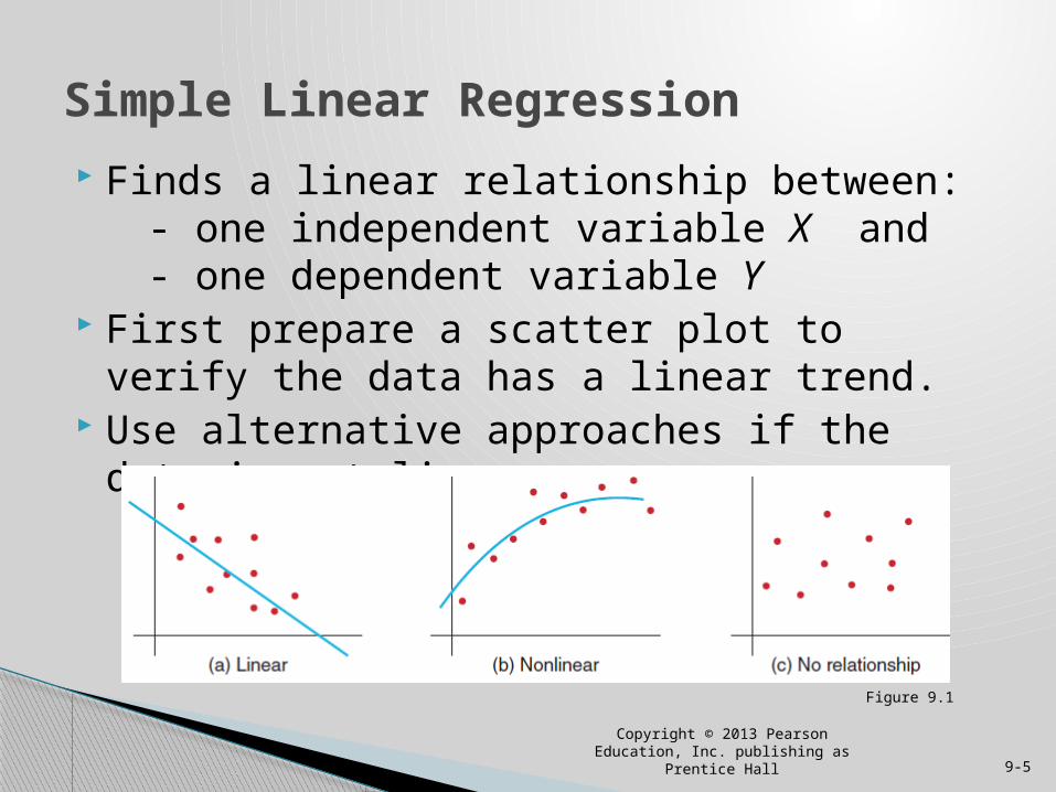
Finds a linear relationship between: - one independent variable X and - one dependent variable Y First prepare a scatter plot to verify the data has a
linear trend. Use alternative approaches if the data is not linear.
Simple Linear Regression
Figure 9.1
Copyright © 2013 Pearson Education, Inc. publishing as Prentice Hall 9-5
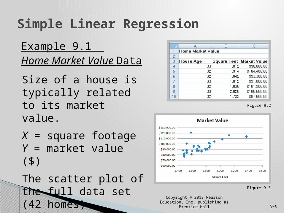
Example 9.1 Home Market Value Data
Simple Linear Regression
Figure 9.2
Copyright © 2013 Pearson Education, Inc. publishing as Prentice Hall 9-6
Figure 9.3
Size of a house is typically related to its market value.
X = square footageY = market value ($)
The scatter plot of the full data set (42 homes) indicates a linear trend.
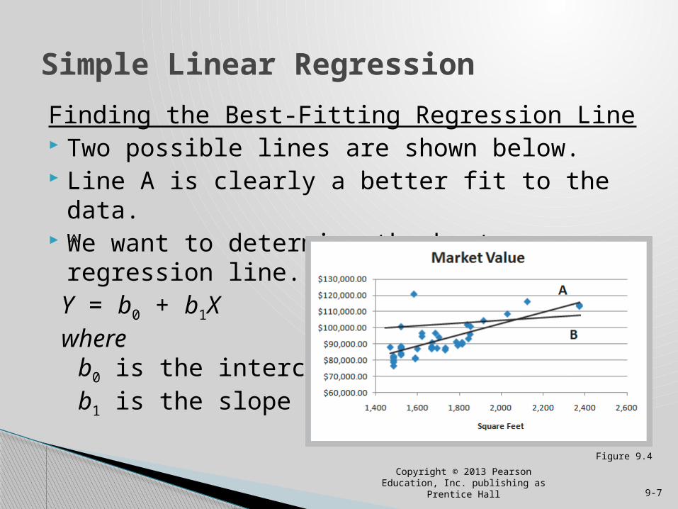
Finding the Best-Fitting Regression Line Two possible lines are shown below. Line A is clearly a better fit to the data. We want to determine the best regression line. Y = b0 + b1X where b0 is the intercept b1 is the slope
Simple Linear Regression
Figure 9.4
Copyright © 2013 Pearson Education, Inc. publishing as Prentice Hall 9-7
^
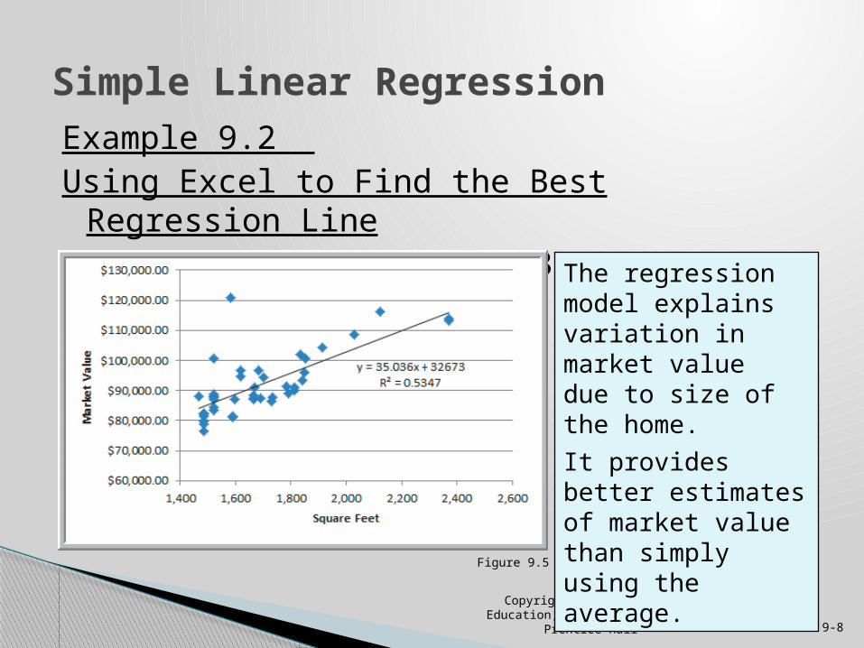
Example 9.2 Using Excel to Find the Best Regression Line Market value = 32673 + 35.036(square feet)
Simple Linear Regression
Figure 9.5
Copyright © 2013 Pearson Education, Inc. publishing as Prentice Hall 9-8
The regression model explains variation in market value due to size of the home.
It provides better estimates of market value than simply using the average.
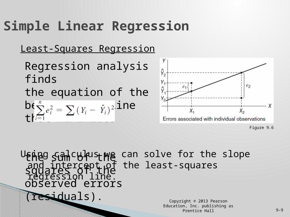
Least-Squares Regression
Using calculus we can solve for the slope and intercept of the least-squares regression line.
Regression analysis finds the equation of the best-fitting line that minimizes
the sum of the squares of the observed errors (residuals).
Simple Linear Regression
Figure 9.6
Copyright © 2013 Pearson Education, Inc. publishing as Prentice Hall 9-9
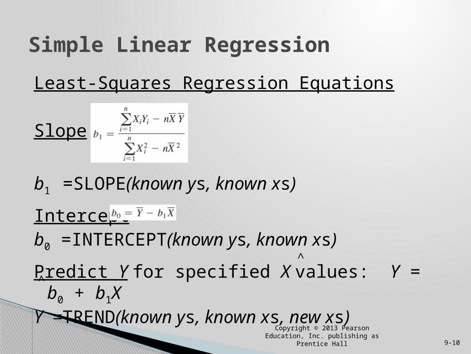
Least-Squares Regression Equations
Slope
b1 =SLOPE(known ys, known xs)
Interceptb0 =INTERCEPT(known ys, known xs)
Predict Y for specified X values: Y = b0 + b1XY =TREND(known ys, known xs, new xs)
Simple Linear Regression
Copyright © 2013 Pearson Education, Inc. publishing as Prentice Hall 9-10
^
^
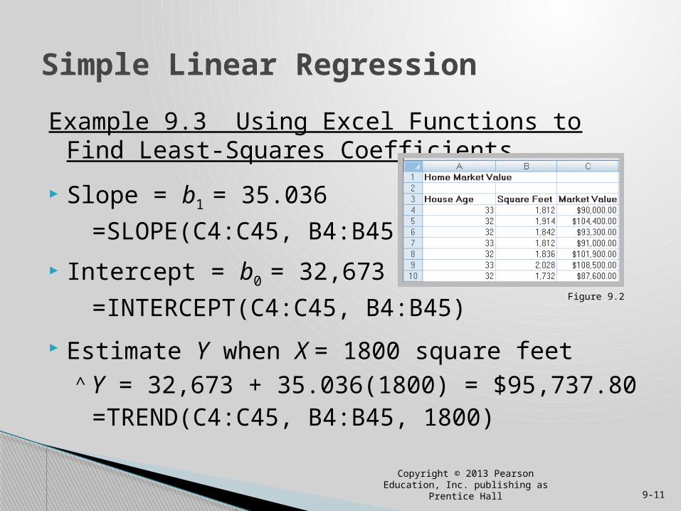
Example 9.3 Using Excel Functions to Find Least-Squares Coefficients
Slope = b1 = 35.036
=SLOPE(C4:C45, B4:B45)
Intercept = b0 = 32,673
=INTERCEPT(C4:C45, B4:B45)
Estimate Y when X = 1800 square feet
Y = 32,673 + 35.036(1800) = $95,737.80 =TREND(C4:C45, B4:B45, 1800)
Simple Linear Regression
Copyright © 2013 Pearson Education, Inc. publishing as Prentice Hall 9-11
Figure 9.2
^
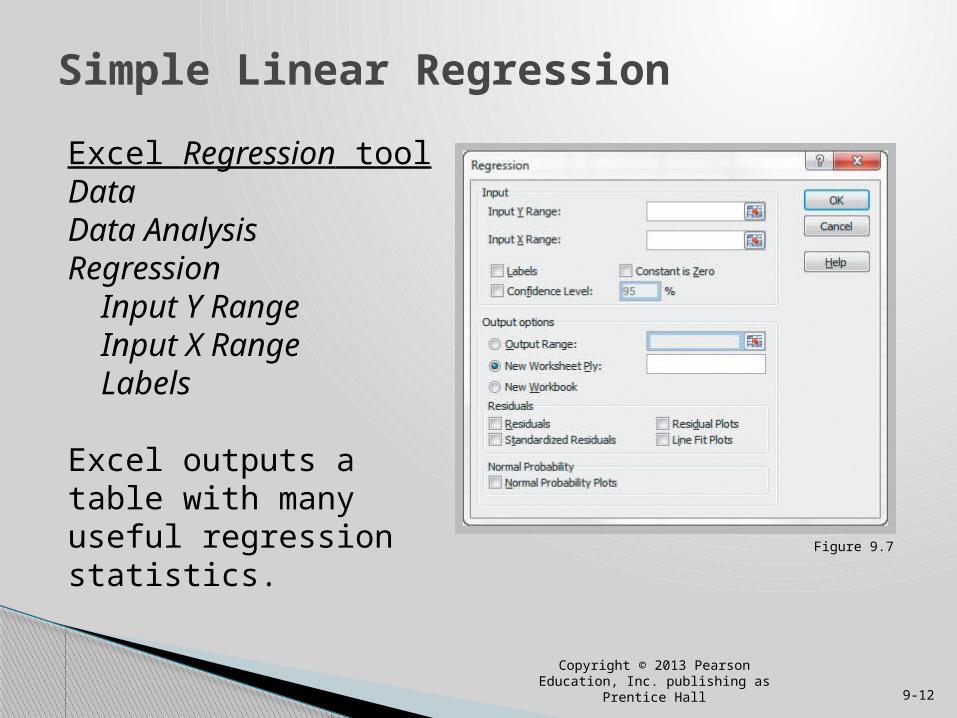
Excel Regression toolDataData AnalysisRegression Input Y Range Input X Range Labels
Excel outputs a table with many useful regression statistics.
Simple Linear Regression
Figure 9.7
Copyright © 2013 Pearson Education, Inc. publishing as Prentice Hall 9-12
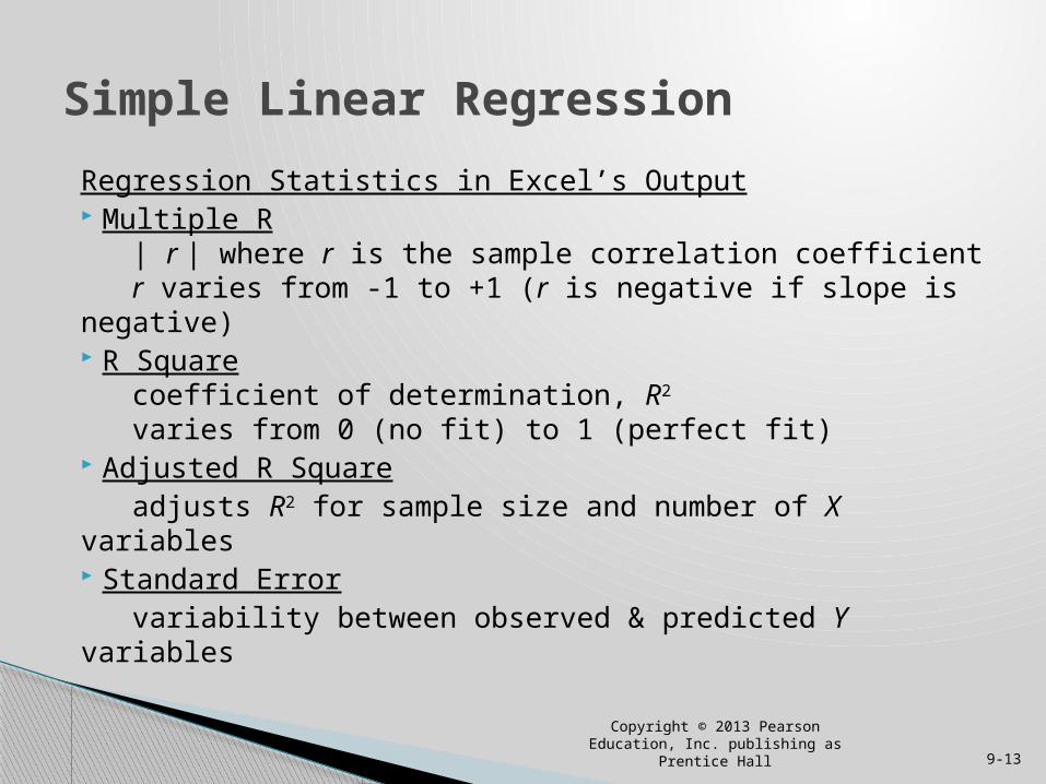
Regression Statistics in Excel’s Output Multiple R | r | where r is the sample correlation coefficient r varies from -1 to +1 (r is negative if slope is negative) R Square coefficient of determination, R2
varies from 0 (no fit) to 1 (perfect fit) Adjusted R Square adjusts R2 for sample size and number of X variables Standard Error variability between observed & predicted Y variables
Simple Linear Regression
Copyright © 2013 Pearson Education, Inc. publishing as Prentice Hall 9-13
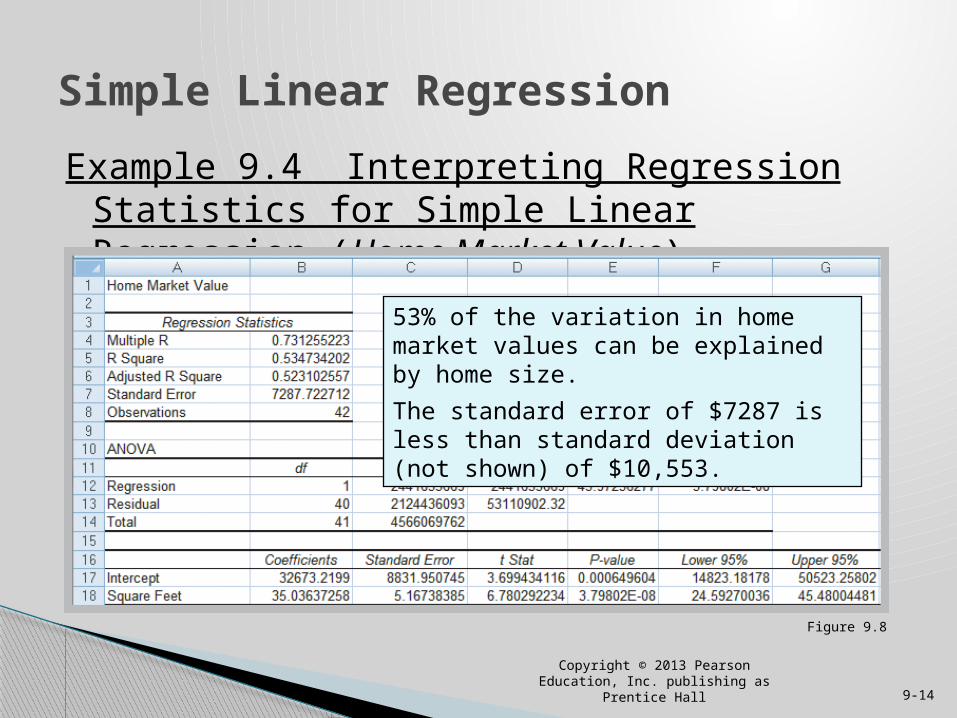
Example 9.4 Interpreting Regression Statistics for Simple Linear Regression (Home Market Value)
Simple Linear Regression
Copyright © 2013 Pearson Education, Inc. publishing as Prentice Hall 9-14
Figure 9.8
53% of the variation in home market values can be explained by home size.
The standard error of $7287 is less than standard deviation (not shown) of $10,553.
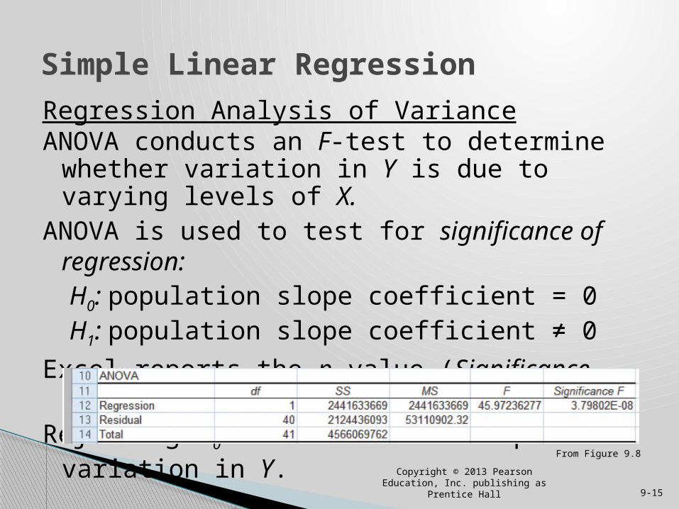
Regression Analysis of VarianceANOVA conducts an F-test to determine whether
variation in Y is due to varying levels of X.ANOVA is used to test for significance of regression: H0: population slope coefficient = 0 H1: population slope coefficient ≠ 0
Excel reports the p-value (Significance F).Rejecting H0 indicates that X explains variation in Y.
Simple Linear Regression
Copyright © 2013 Pearson Education, Inc. publishing as Prentice Hall 9-15
From Figure 9.8
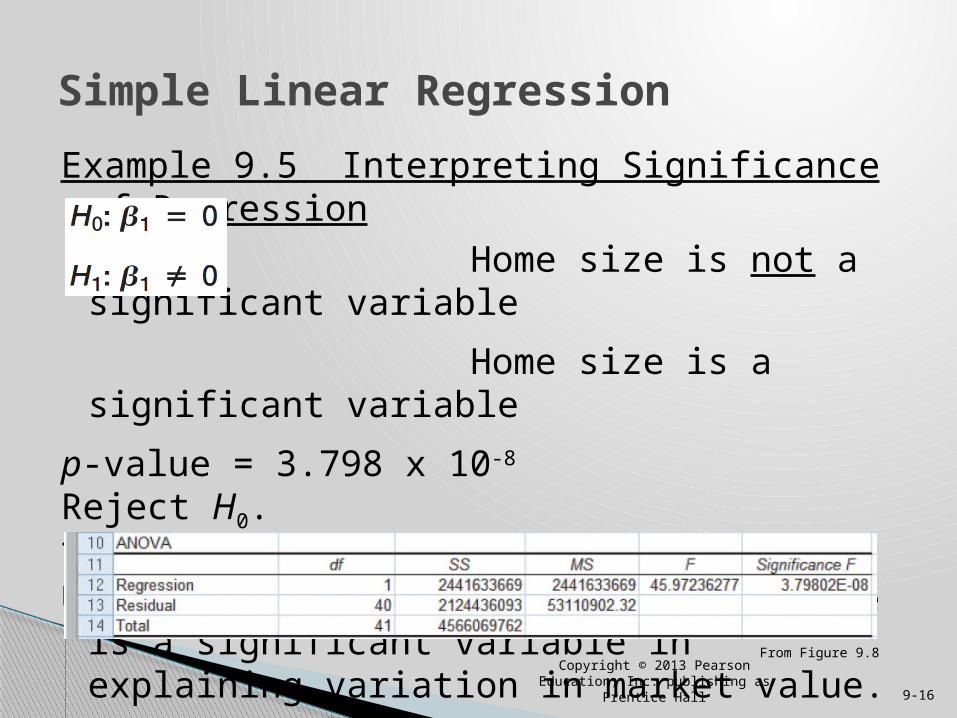
Example 9.5 Interpreting Significance of Regression
Home size is not a significant variable
Home size is a significant variable
p-value = 3.798 x 10⁻⁸
Reject H0.The slope is not equal to zero.Using a linear relationship, home size is a significant
variable in explaining variation in market value.
Simple Linear Regression
Copyright © 2013 Pearson Education, Inc. publishing as Prentice Hall 9-16
From Figure 9.8
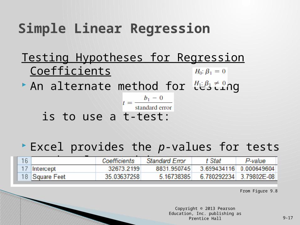
Testing Hypotheses for Regression Coefficients An alternate method for testing
is to use a t-test:
Excel provides the p-values for tests on the slope and intercept.
Simple Linear Regression
Copyright © 2013 Pearson Education, Inc. publishing as Prentice Hall 9-17
From Figure 9.8
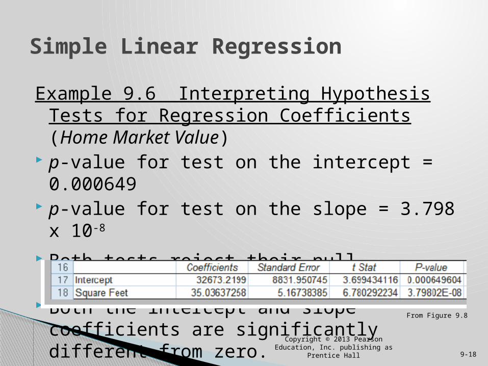
Example 9.6 Interpreting Hypothesis Tests for Regression Coefficients (Home Market Value)
p-value for test on the intercept = 0.000649 p-value for test on the slope = 3.798 x 10⁻⁸
Both tests reject their null hypotheses. Both the intercept and slope coefficients are
significantly different from zero.
Simple Linear Regression
Copyright © 2013 Pearson Education, Inc. publishing as Prentice Hall 9-18
From Figure 9.8
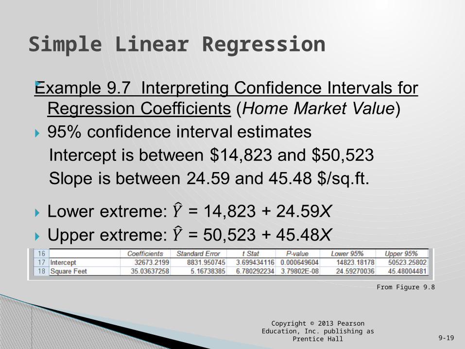
Simple Linear Regression
Copyright © 2013 Pearson Education, Inc. publishing as Prentice Hall 9-19
From Figure 9.8
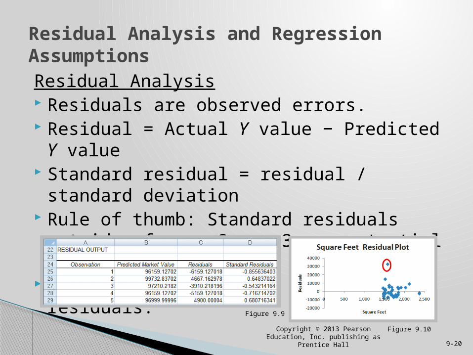
Residual Analysis Residuals are observed errors. Residual = Actual Y value − Predicted Y value Standard residual = residual / standard deviation Rule of thumb: Standard residuals outside of ±2
or ±3 are potential outliers. Excel provides a table and a plot of residuals.
Residual Analysis and Regression Assumptions
Copyright © 2013 Pearson Education, Inc. publishing as Prentice Hall 9-20
Figure 9.10
Figure 9.9
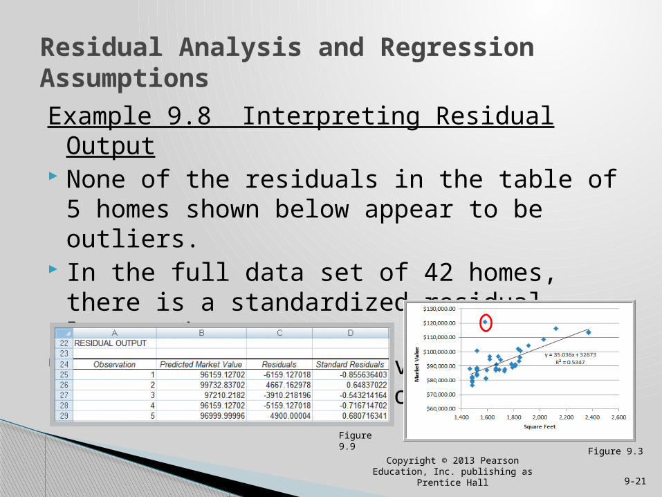
Example 9.8 Interpreting Residual Output None of the residuals in the table of 5 homes
shown below appear to be outliers. In the full data set of 42 homes, there is a
standardized residual larger than 4. This small home may have a pool or unusually
large piece of land.
Residual Analysis and Regression Assumptions
Copyright © 2013 Pearson Education, Inc. publishing as Prentice Hall 9-21
Figure 9.9
Figure 9.3
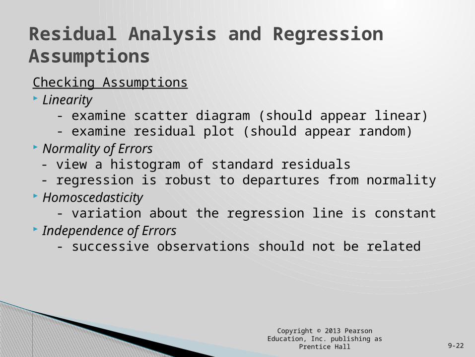
Checking Assumptions Linearity - examine scatter diagram (should appear linear) - examine residual plot (should appear random) Normality of Errors - view a histogram of standard residuals - regression is robust to departures from normality Homoscedasticity - variation about the regression line is constant Independence of Errors - successive observations should not be related
Residual Analysis and Regression Assumptions
Copyright © 2013 Pearson Education, Inc. publishing as Prentice Hall 9-22
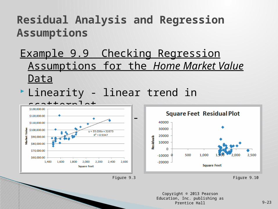
Example 9.9 Checking Regression Assumptions for the Home Market Value Data
Linearity - linear trend in scatterplot - no pattern in residual plot
Residual Analysis and Regression Assumptions
Copyright © 2013 Pearson Education, Inc. publishing as Prentice Hall 9-23
Figure 9.10Figure 9.3
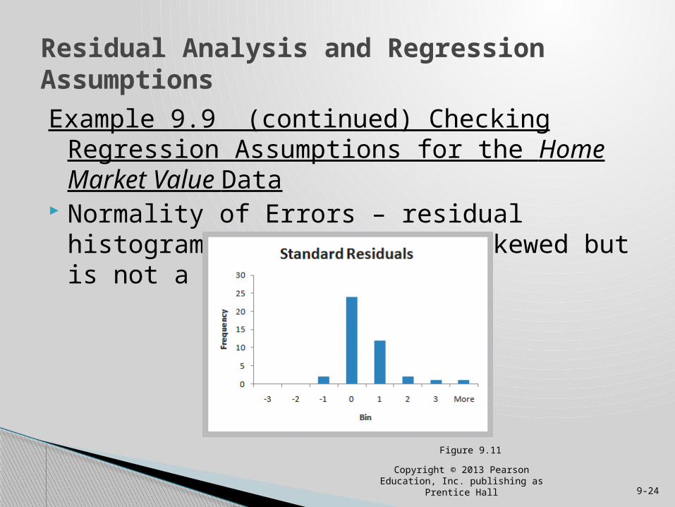
Example 9.9 (continued) Checking Regression Assumptions for the Home Market Value Data
Normality of Errors – residual histogram appears slightly skewed but is not a serious departure
Residual Analysis and Regression Assumptions
Copyright © 2013 Pearson Education, Inc. publishing as Prentice Hall 9-24
Figure 9.11
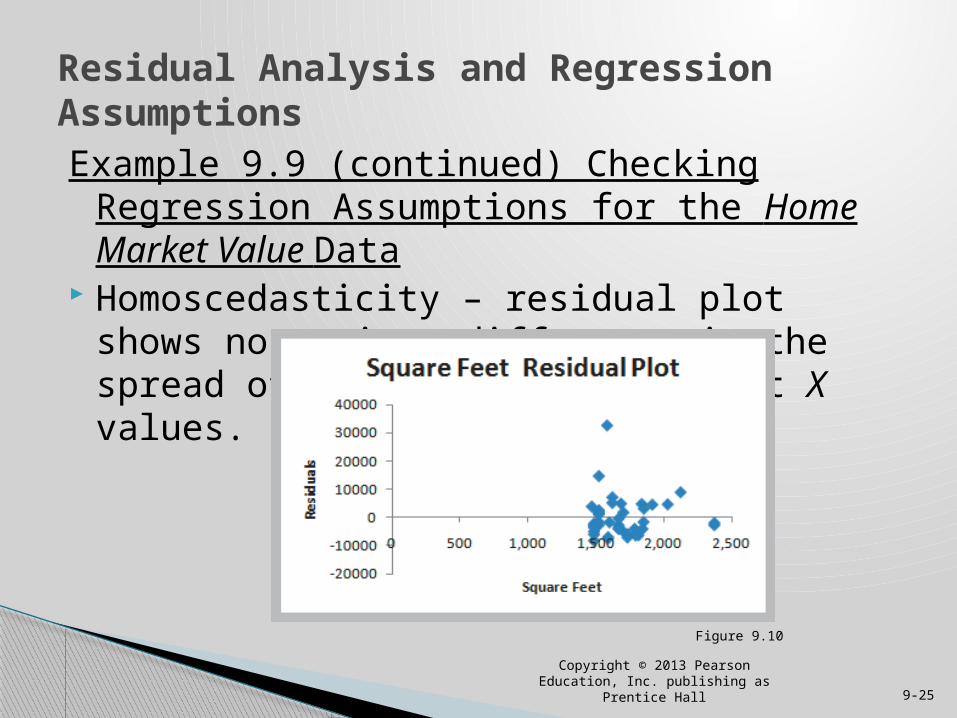
Example 9.9 (continued) Checking Regression Assumptions for the Home Market Value Data
Homoscedasticity – residual plot shows no serious difference in the spread of the data for different X values.
Residual Analysis and Regression Assumptions
Copyright © 2013 Pearson Education, Inc. publishing as Prentice Hall 9-25
Figure 9.10
Example 9.9 (continued) Checking Regression Assumptions for the Home Market Value Data
Independence of Errors – Because the data is cross-sectional, we can assume this assumption holds.
All 4 regression assumptions are reasonable for the Home Market Value data.
Residual Analysis and Regression Assumptions
Copyright © 2013 Pearson Education, Inc. publishing as Prentice Hall 9-26
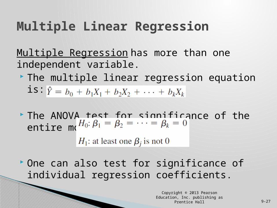
Multiple Regression has more than one independent variable. The multiple linear regression equation is:
The ANOVA test for significance of the entire model is:
One can also test for significance of individual regression coefficients.
Multiple Linear Regression
Copyright © 2013 Pearson Education, Inc. publishing as Prentice Hall 9-27
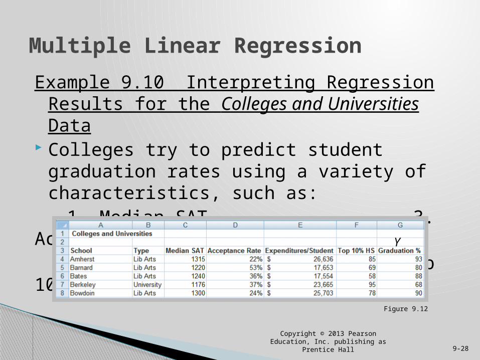
Example 9.10 Interpreting Regression Results for the Colleges and Universities Data
Colleges try to predict student graduation rates using a variety of characteristics, such as:
1. Median SAT 3. Acceptance rate 2. Expenditures/student 4. Top 10% of HS class
Multiple Linear Regression
Figure 9.12
Copyright © 2013 Pearson Education, Inc. publishing as Prentice Hall 9-28
Y
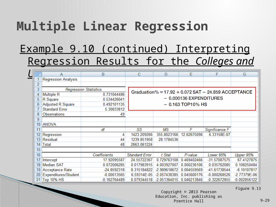
Example 9.10 (continued) Interpreting Regression Results for the Colleges and Universities Data
Multiple Linear Regression
Copyright © 2013 Pearson Education, Inc. publishing as Prentice Hall 9-29
Figure 9.13
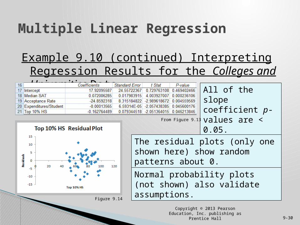
Example 9.10 (continued) Interpreting Regression Results for the Colleges and Universities Data
Multiple Linear Regression
Figure 9.14
Copyright © 2013 Pearson Education, Inc. publishing as Prentice Hall 9-30
All of the slope coefficient p-values are < 0.05.
The residual plots (only one shown here) show random patterns about 0.
From Figure 9.13
Normal probability plots (not shown) also validate assumptions.
Analytics in Practice: Using Linear Regression and Interactive Risk Simulators to Predict Performance at ARAMARK ARAMARK, located in Philadelphia, is an award-
winning provider of professional services They developed an on-line tool called “interactive
risk simulators” (shown on next slide) that allows users to change various business metrics and immediately see the results.
The simulators use linear regression models.
Copyright © 2013 Pearson Education, Inc. publishing as Prentice Hall 9-31
Multiple Linear Regression
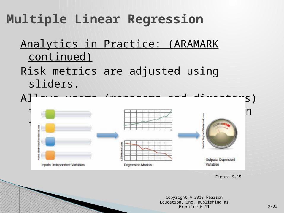
Analytics in Practice: (ARAMARK continued)Risk metrics are adjusted using sliders.Allows users (managers and directors) to see the
impact of these risks on the business.
Copyright © 2013 Pearson Education, Inc. publishing as Prentice Hall 9-32
Figure 9.15
Multiple Linear Regression
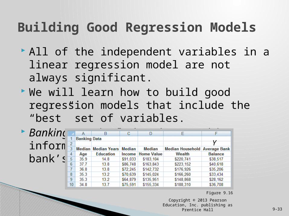
All of the independent variables in a linear regression model are not always significant.
We will learn how to build good regression models that include the “best” set of variables.
Banking Data includes demographic information on customers in the bank’s current market.
Building Good Regression Models
Figure 9.16
Copyright © 2013 Pearson Education, Inc. publishing as Prentice Hall 9-33
Y
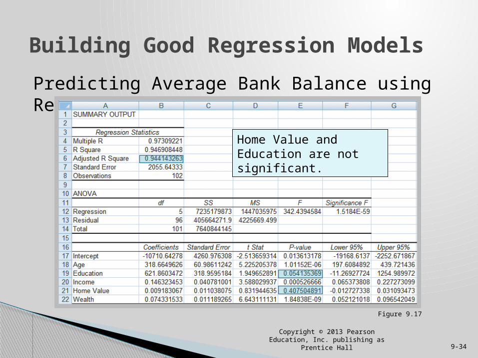
Predicting Average Bank Balance using Regression
Building Good Regression Models
Figure 9.17
Copyright © 2013 Pearson Education, Inc. publishing as Prentice Hall 9-34
Home Value and Education are not significant.
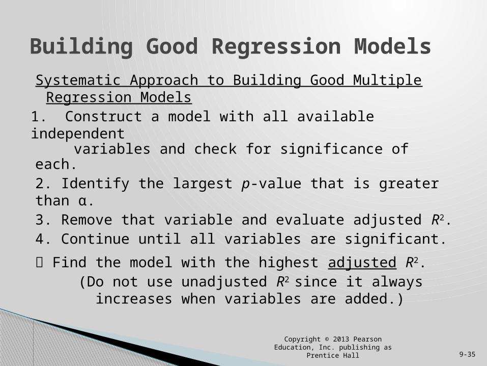
Systematic Approach to Building Good Multiple Regression Models
1. Construct a model with all available independent variables and check for significance of each.2. Identify the largest p-value that is greater than α.3. Remove that variable and evaluate adjusted R2.4. Continue until all variables are significant.
Find the model with the highest adjusted R2. (Do not use unadjusted R2 since it always increases when variables are added.)
Building Good Regression Models
Copyright © 2013 Pearson Education, Inc. publishing as Prentice Hall 9-35
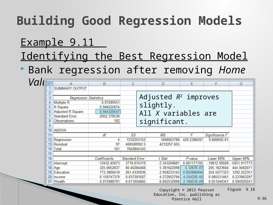
Example 9.11 Identifying the Best Regression Model Bank regression after removing Home Value
Building Good Regression Models
Figure 9.18Copyright © 2013 Pearson Education, Inc.
publishing as Prentice Hall 9-36
Adjusted R2 improves slightly. All X variables are significant.
Multicollinearity- occurs when there are strong correlations among the independent variables- makes it difficult to isolate the effects of independent variables- signs of slope coefficients may be opposite of the true value and p-values can be inflated
Correlations exceeding ±0.7 are an indication that multicollinearity might exist.
Variance Inflation Factors are a better indicator. Parsimony is an age-old principle that applies here.
Building Good Regression Models
Copyright © 2013 Pearson Education, Inc. publishing as Prentice Hall 9-37
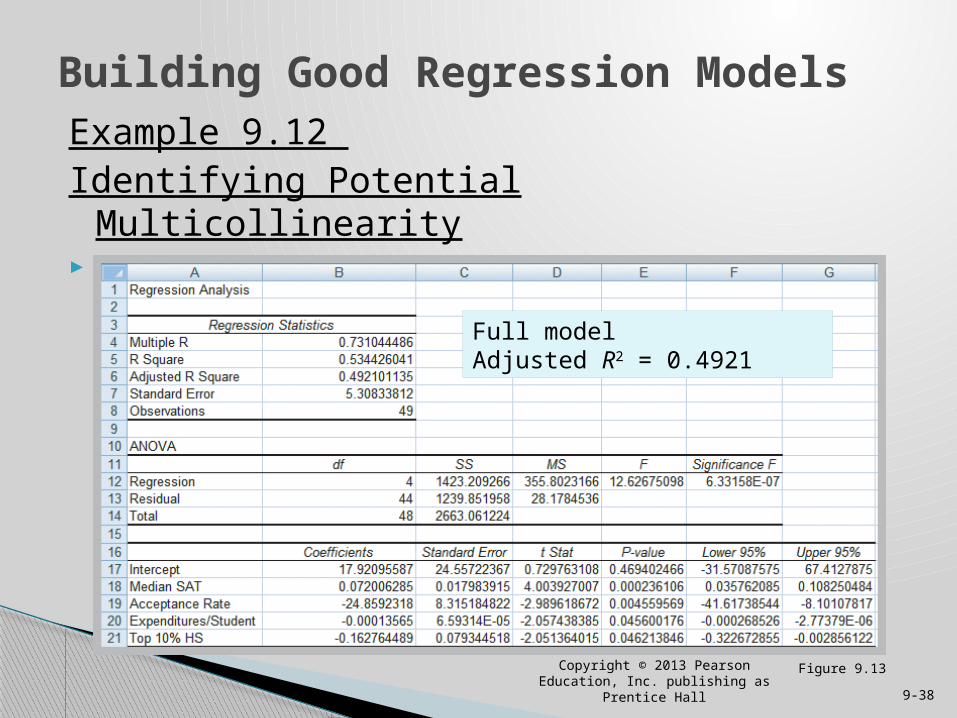
Example 9.12 Identifying Potential Multicollinearity Colleges and Universities (full model)
Building Good Regression Models
Copyright © 2013 Pearson Education, Inc. publishing as Prentice Hall 9-38
Figure 9.13
Full modelAdjusted R2 = 0.4921
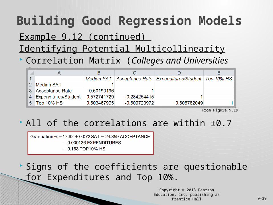
Example 9.12 (continued) Identifying Potential Multicollinearity Correlation Matrix (Colleges and Universities data)
All of the correlations are within ±0.7
Signs of the coefficients are questionable for Expenditures and Top 10%.
Building Good Regression Models
From Figure 9.19
Copyright © 2013 Pearson Education, Inc. publishing as Prentice Hall 9-39

Example 9.12 (continued) Identifying Potential Multicollinearity Colleges and Universities (reduced model)
Building Good Regression Models
Copyright © 2013 Pearson Education, Inc. publishing as Prentice Hall 9-40
Dropping Top 10%Adjusted R2 drops to 0.4559
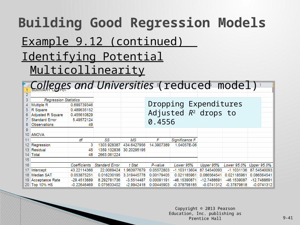
Example 9.12 (continued) Identifying Potential Multicollinearity Colleges and Universities (reduced model)
Building Good Regression Models
Copyright © 2013 Pearson Education, Inc. publishing as Prentice Hall 9-41
Dropping ExpendituresAdjusted R2 drops to 0.4556
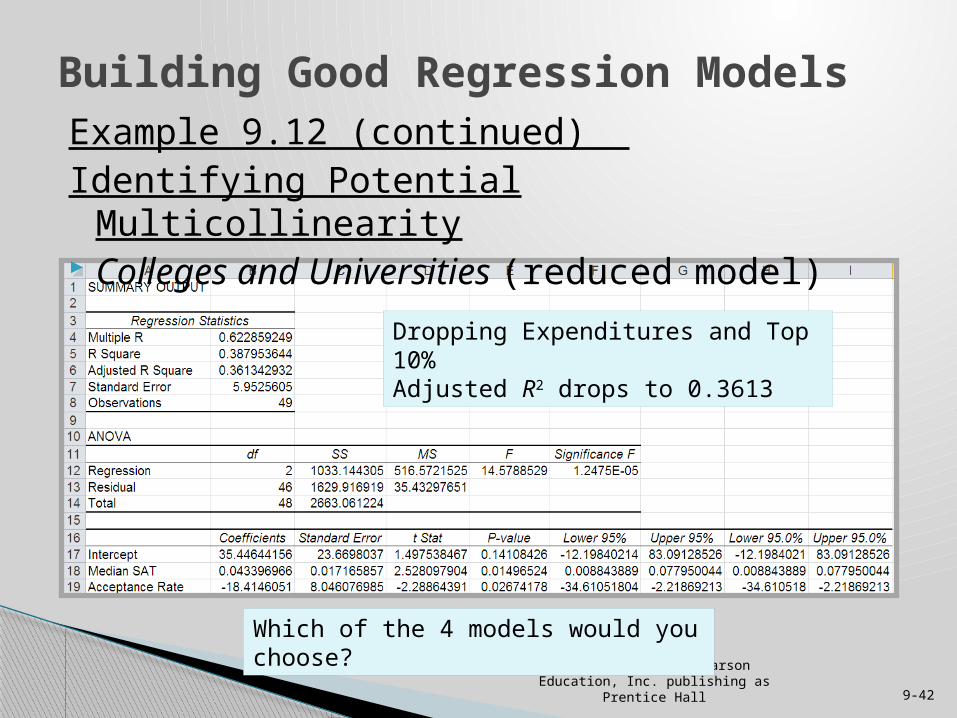
Example 9.12 (continued) Identifying Potential Multicollinearity Colleges and Universities (reduced model)
Building Good Regression Models
Copyright © 2013 Pearson Education, Inc. publishing as Prentice Hall 9-42
Dropping Expenditures and Top 10%Adjusted R2 drops to 0.3613
Which of the 4 models would you choose?
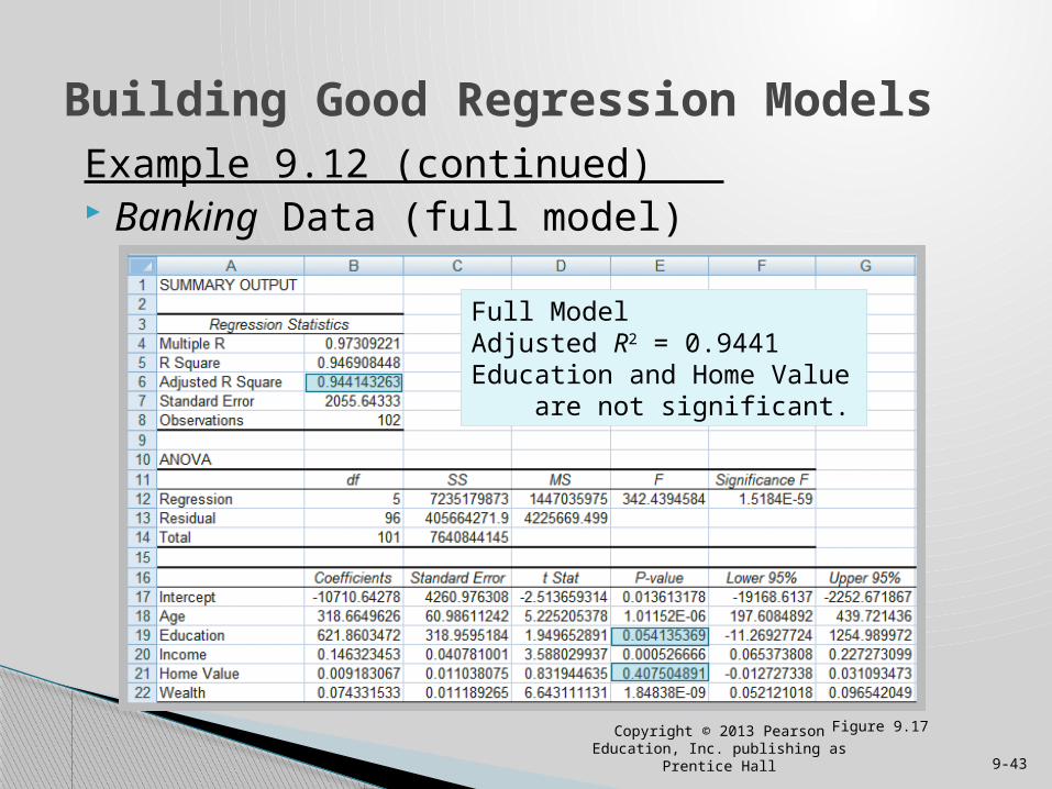
Figure 9.17
Example 9.12 (continued) Banking Data (full model)
Building Good Regression Models
Copyright © 2013 Pearson Education, Inc. publishing as Prentice Hall 9-43
Full ModelAdjusted R2 = 0.9441Education and Home Value are not significant.
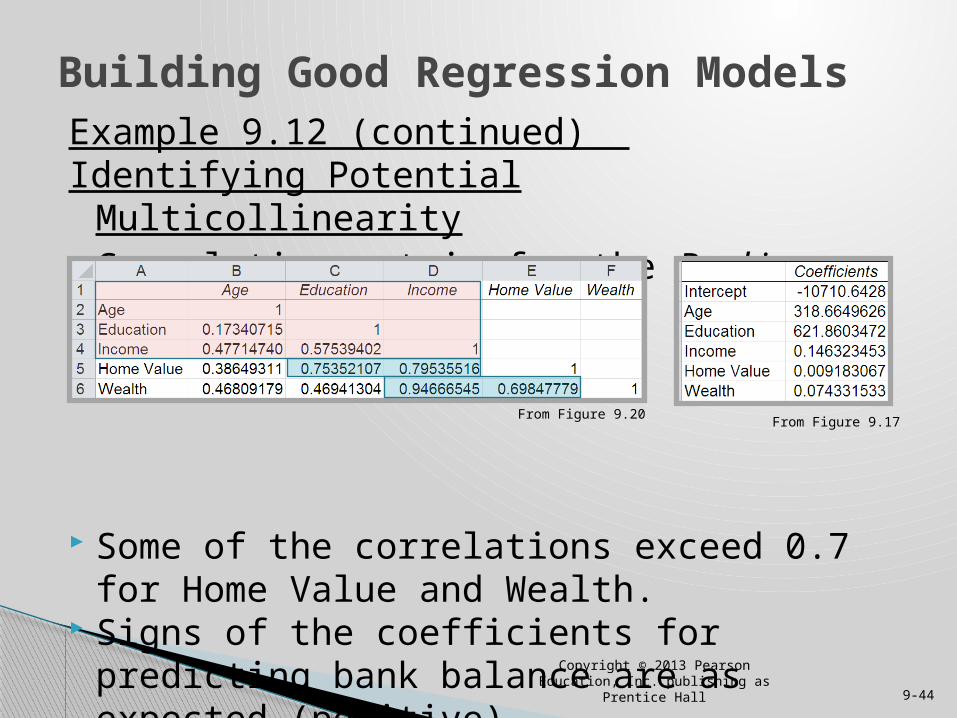
Example 9.12 (continued) Identifying Potential Multicollinearity Correlation matrix for the Banking data
Some of the correlations exceed 0.7 for Home Value and Wealth.
Signs of the coefficients for predicting bank balance are as expected (positive).
Building Good Regression Models
Copyright © 2013 Pearson Education, Inc. publishing as Prentice Hall 9-44
From Figure 9.20From Figure 9.17
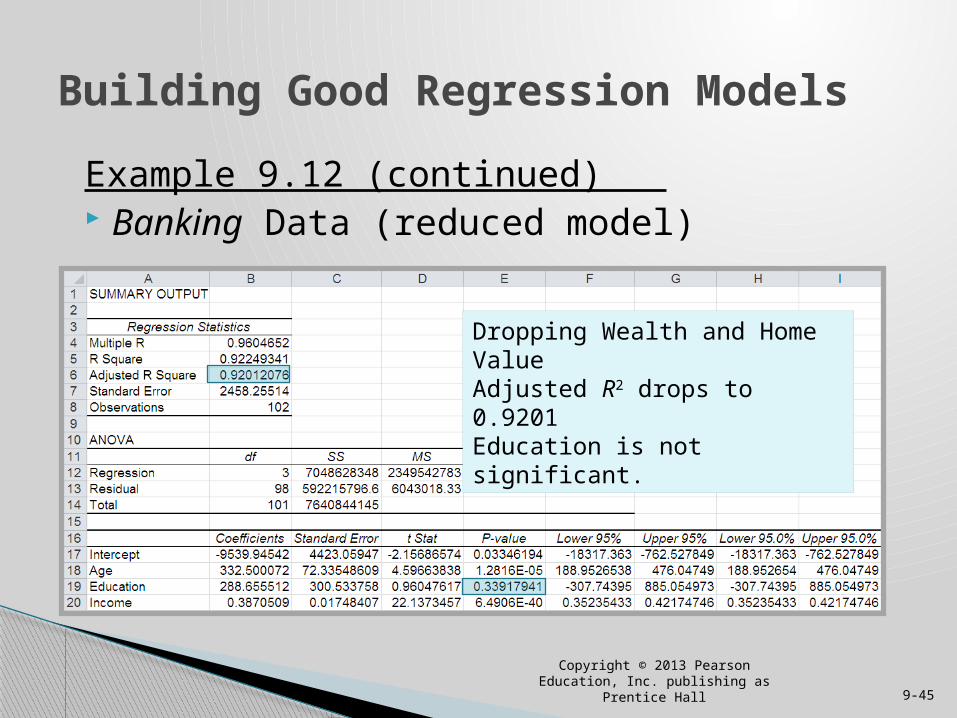
Example 9.12 (continued) Banking Data (reduced model)
Building Good Regression Models
Copyright © 2013 Pearson Education, Inc. publishing as Prentice Hall 9-45
Dropping Wealth and Home ValueAdjusted R2 drops to 0.9201Education is not significant.
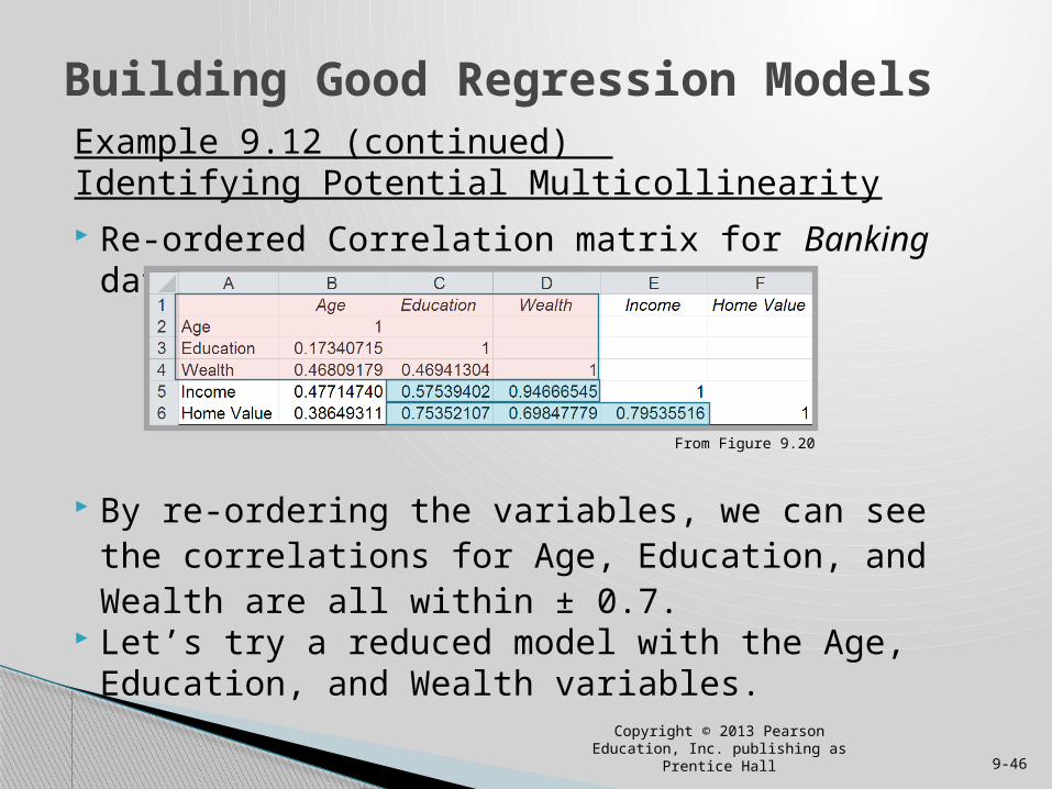
Example 9.12 (continued) Identifying Potential Multicollinearity
Re-ordered Correlation matrix for Banking data
By re-ordering the variables, we can see the correlations for Age, Education, and Wealth are all within ± 0.7.
Let’s try a reduced model with the Age, Education, and Wealth variables.
Building Good Regression Models
Copyright © 2013 Pearson Education, Inc. publishing as Prentice Hall 9-46
From Figure 9.20
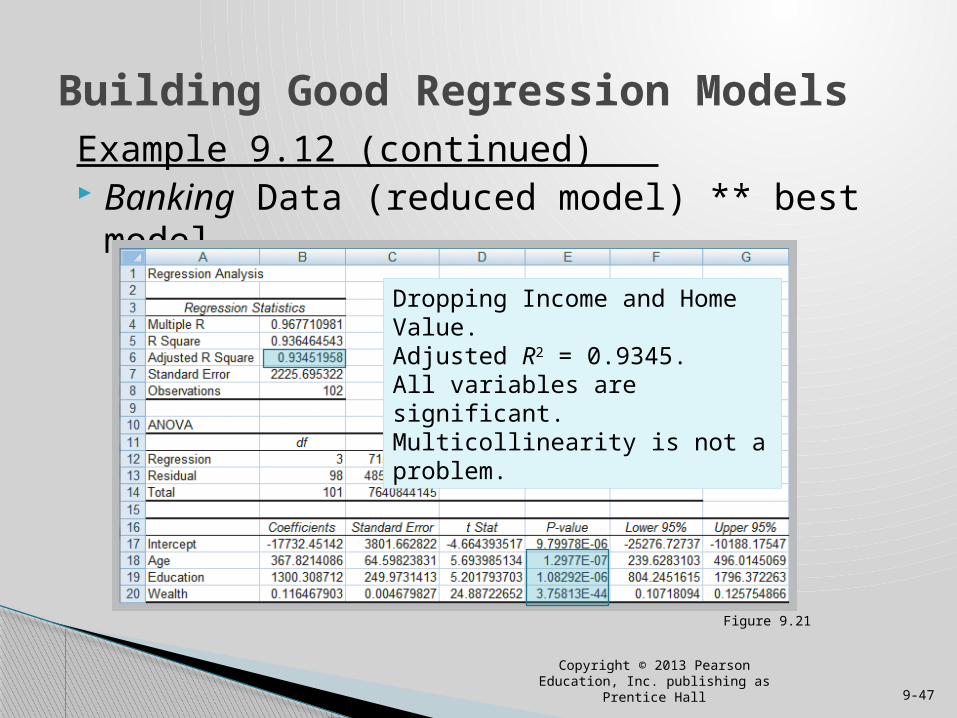
Example 9.12 (continued) Banking Data (reduced model) ** best model
Building Good Regression Models
Copyright © 2013 Pearson Education, Inc. publishing as Prentice Hall 9-47
Figure 9.21
Dropping Income and Home Value.Adjusted R2 = 0.9345.All variables are significant. Multicollinearity is not a problem.
Dealing with Categorical Variables Must be coded numeric using dummy variables. For variables with 2 categories, code as 0 and 1. For variables with k ≥ 3 categories, create k−1
binary (0,1) variables.
Interaction Terms A dependence between two variables is called
interaction. Test for interaction by adding a new term to the
model, such as X3 = X1X2.
Regression with Categorical Variables
Copyright © 2013 Pearson Education, Inc. publishing as Prentice Hall 9-48
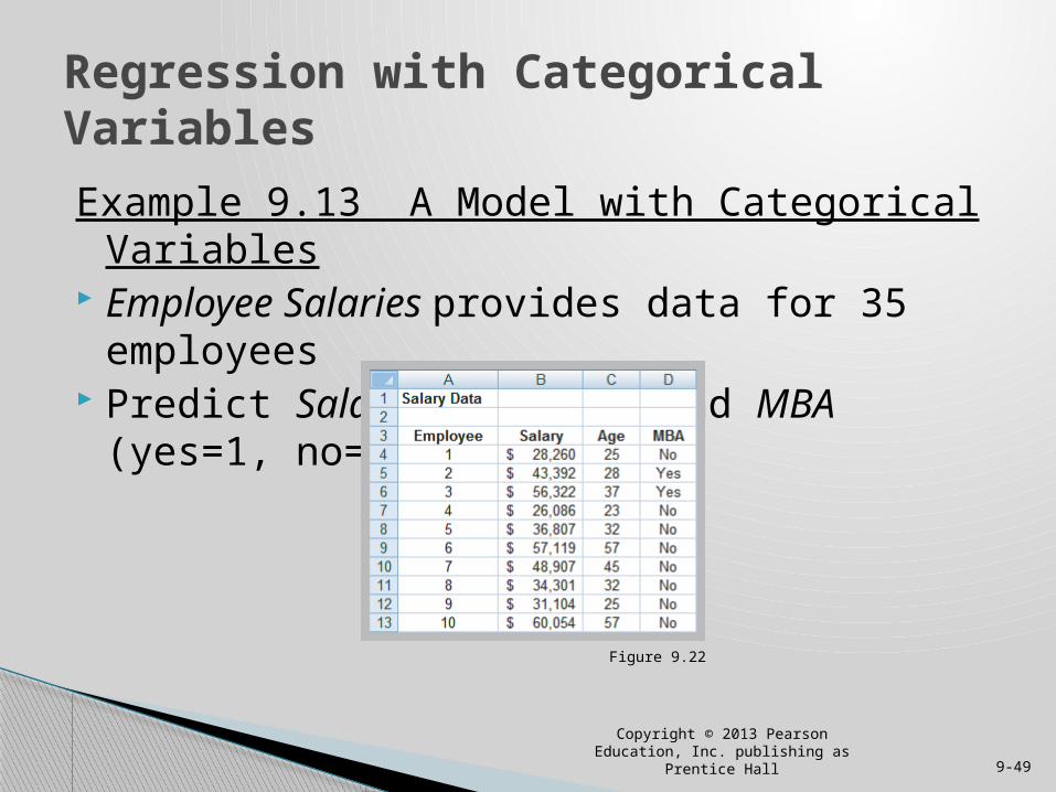
Example 9.13 A Model with Categorical Variables Employee Salaries provides data for 35 employees Predict Salary using Age and MBA (yes=1, no=0)
Regression with Categorical Variables
Figure 9.22
Copyright © 2013 Pearson Education, Inc. publishing as Prentice Hall 9-49
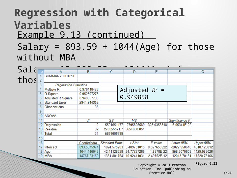
Example 9.13 (continued) Salary = 893.59 + 1044(Age) for those without MBASalary =15,660.82 + 1044(Age) for those with MBA
Regression with Categorical Variables
Figure 9.23
Copyright © 2013 Pearson Education, Inc. publishing as Prentice Hall 9-50
Adjusted R2 = 0.949858
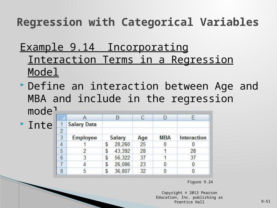
Example 9.14 Incorporating Interaction Terms in a Regression Model
Define an interaction between Age and MBA and include in the regression model.
Interaction = (Age)(MBA)
Figure 9.24
Copyright © 2013 Pearson Education, Inc. publishing as Prentice Hall 9-51
Regression with Categorical Variables
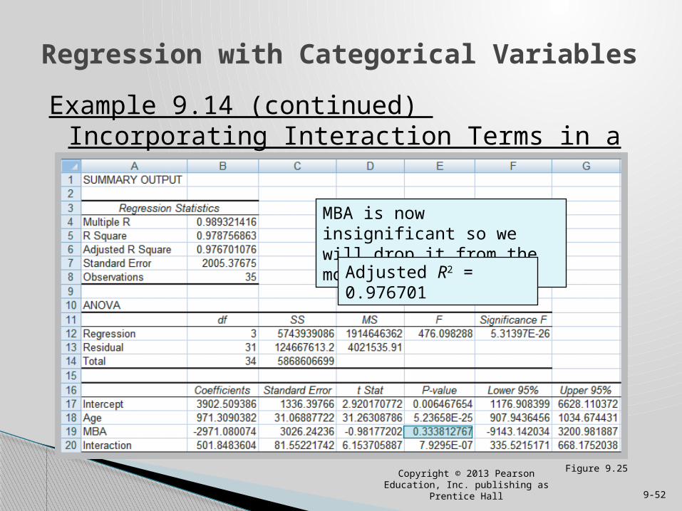
Example 9.14 (continued) Incorporating Interaction Terms in a Regression Model
Figure 9.25
Copyright © 2013 Pearson Education, Inc. publishing as Prentice Hall 9-52
Regression with Categorical Variables
MBA is now insignificant so we will drop it from the model.
Adjusted R2 = 0.976701
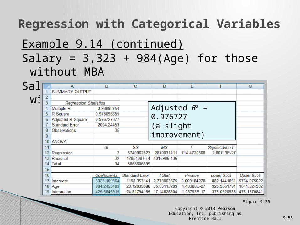
Example 9.14 (continued)Salary = 3,323 + 984(Age) for those without MBASalary = 3,323 + 1410(Age) for those with MBA
Figure 9.26
Copyright © 2013 Pearson Education, Inc. publishing as Prentice Hall 9-53
Regression with Categorical Variables
Adjusted R2 = 0.976727(a slight improvement)
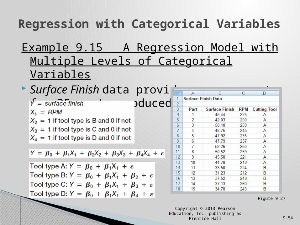
Example 9.15 A Regression Model with Multiple Levels of Categorical Variables
Surface Finish data provides measurements for 35 parts produced on a lathe.
Copyright © 2013 Pearson Education, Inc. publishing as Prentice Hall 9-54
Regression with Categorical Variables
Figure 9.27
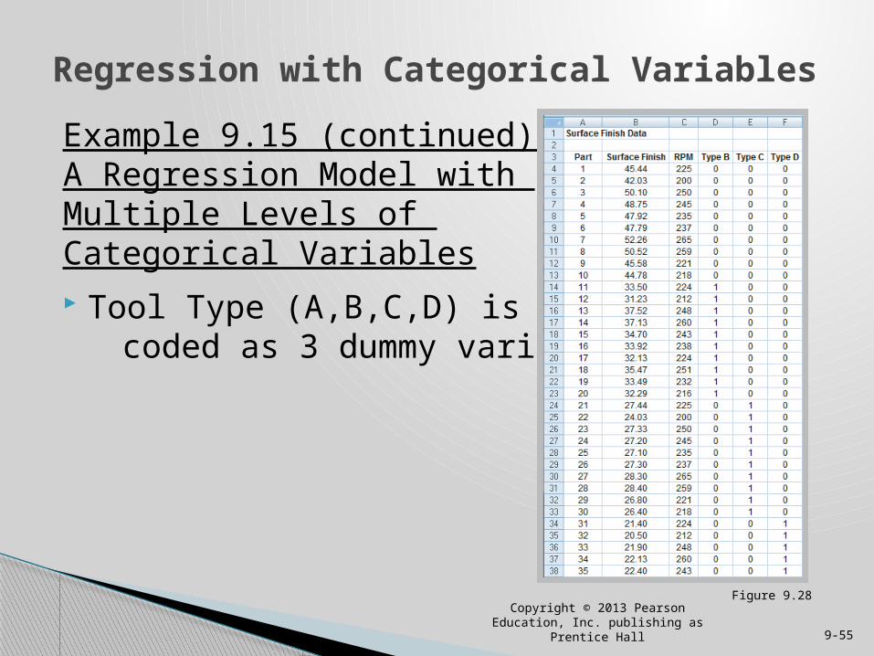
Example 9.15 (continued) A Regression Model with Multiple Levels of Categorical Variables
Tool Type (A,B,C,D) is now coded as 3 dummy variables
Figure 9.28
Copyright © 2013 Pearson Education, Inc. publishing as Prentice Hall 9-55
Regression with Categorical Variables
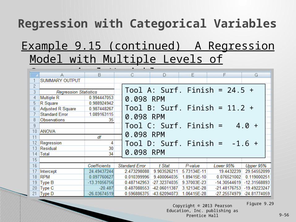
Example 9.15 (continued) A Regression Model with Multiple Levels of Categorical Variables
Figure 9.29
Copyright © 2013 Pearson Education, Inc. publishing as Prentice Hall 9-56
Regression with Categorical Variables
Tool A: Surf. Finish = 24.5 + 0.098 RPMTool B: Surf. Finish = 11.2 + 0.098 RPMTool C: Surf. Finish = 4.0 + 0.098 RPMTool D: Surf. Finish = -1.6 + 0.098 RPM
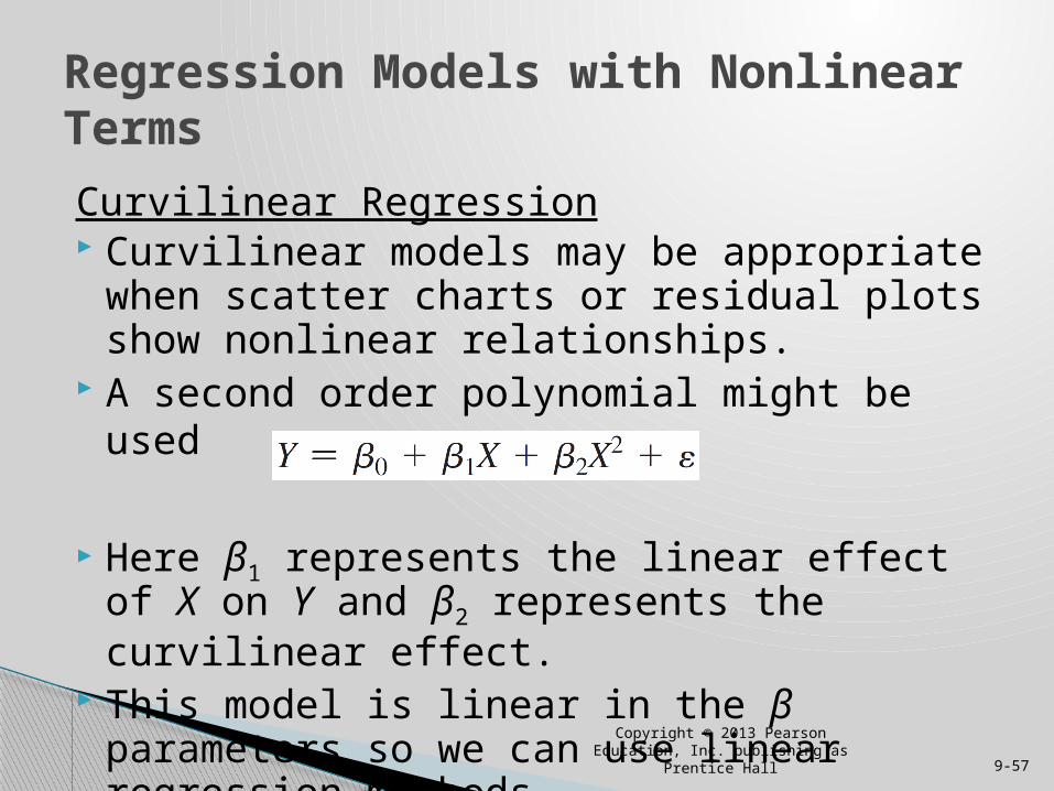
Curvilinear Regression Curvilinear models may be appropriate when
scatter charts or residual plots show nonlinear relationships.
A second order polynomial might be used
Here β1 represents the linear effect of X on Y and β2 represents the curvilinear effect. This model is linear in the β parameters so we can
use linear regression methods.
Regression Models with Nonlinear Terms
Copyright © 2013 Pearson Education, Inc. publishing as Prentice Hall 9-57
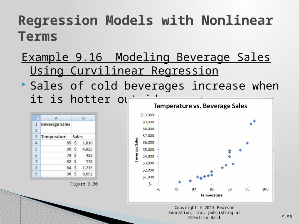
Example 9.16 Modeling Beverage Sales Using Curvilinear Regression
Sales of cold beverages increase when it is hotter outside.
Regression Models with Nonlinear Terms
Figure 9.30
Copyright © 2013 Pearson Education, Inc. publishing as Prentice Hall 9-58
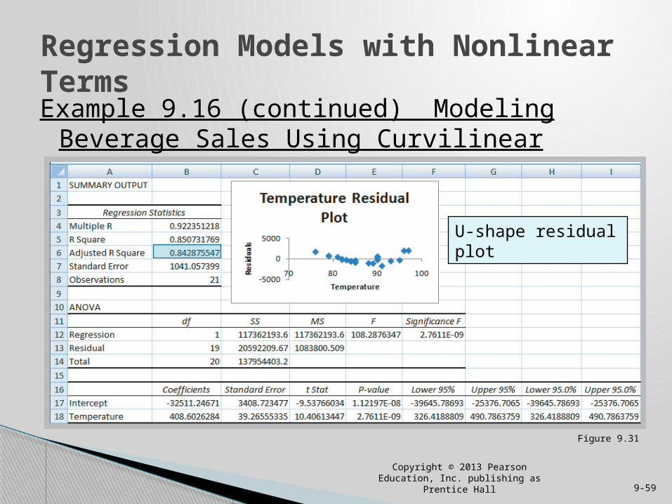
Example 9.16 (continued) Modeling Beverage Sales Using Curvilinear Regression
Regression Models with Nonlinear Terms
Figure 9.31
Copyright © 2013 Pearson Education, Inc. publishing as Prentice Hall 9-59
U-shape residual plot
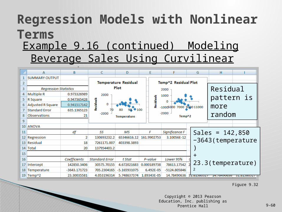
Example 9.16 (continued) Modeling Beverage Sales Using Curvilinear Regression
Regression Models with Nonlinear Terms
Figure 9.32
Copyright © 2013 Pearson Education, Inc. publishing as Prentice Hall 9-60
Sales = 142,850−3643(temperature)+ 23.3(temperature)2
Residual pattern is more random
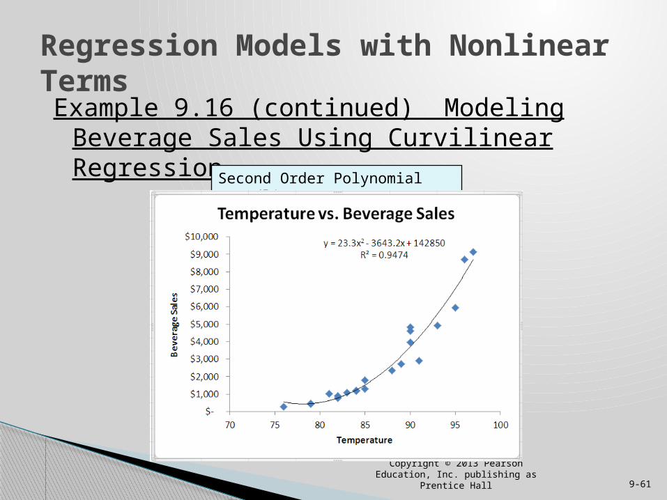
Example 9.16 (continued) Modeling Beverage Sales Using Curvilinear Regression
Regression Models with Nonlinear Terms
Copyright © 2013 Pearson Education, Inc. publishing as Prentice Hall 9-61
Second Order Polynomial Trendline
Autocorrelation Coefficient of determination Coefficient of multiple determination Curvilinear regression model Dummy variables Homoscedasticity Interaction Least-squares regression Mulitcollinearity Multiple correlation coefficient
Copyright © 2013 Pearson Education, Inc. publishing as Prentice Hall 9-62
Chapter 9 - Key Terms
Multiple linear regression Parsimony Partial regression coefficient Regression analysis Residuals Significance of regression Simple linear regression Standard error of the estimate Standard residuals
Copyright © 2013 Pearson Education, Inc. publishing as Prentice Hall 9-63
Chapter 9 - Key Terms (continued)

Copyright © 2013 Pearson Education, Inc. publishing as Prentice Hall 9-64
Recall that PLE produces lawnmowers and a medium size diesel power lawn tractor.
Predict what might have happened if PLE never implemented the 2009 defect reduction initiative.
Determine the effect of education, GPA, and age when hired on employee retention.
Investigate the rate of learning following the implementation of the new production technology.
Write a formal report summarizing your results.
Case Study Performance Lawn Equipment (9)
Copyright © 2013 Pearson Education, Inc. publishing as Prentice Hall 9-65