Embed Size (px)
Citation preview
BUS41100 Applied Regression Analysis
Week 3: Multiple Linear Regression
Polynomial regression, categorical variables,interactions & main effects, R2
Max H. FarrellThe University of Chicago Booth School of Business
Multiple vs simple linear regression
Fundamental model is the same.
Basic concepts and techniques translate directly from SLR.
I Individual parameter inference and estimation is the same,
conditional on the rest of the model.
I We still use lm, summary, predict, etc.
The hardest part would be moving to matrix algebra to
translate all of our equations. Luckily, R does all that for you.
1
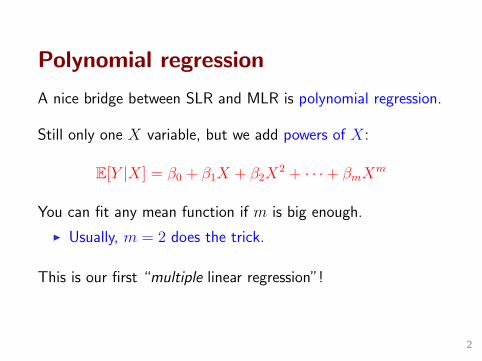
Polynomial regression
A nice bridge between SLR and MLR is polynomial regression.
Still only one X variable, but we add powers of X:
E[Y |X] = β0 + β1X + β2X2 + · · ·+ βmX
m
You can fit any mean function if m is big enough.
I Usually, m = 2 does the trick.
This is our first “multiple linear regression”!
2

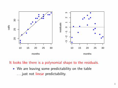
Example: telemarketing/call-center data.
I How does length of employment (months) relate to
productivity (number of calls placed per day)?
> attach(telemkt <- read.csv("telemarketing.csv"))
> tele1 <- lm(calls~months)
> xgrid <- data.frame(months = 10:30)
> par(mfrow=c(1,2))
> plot(months, calls, pch=20, col=4)
> lines(xgrid$months, predict(tele1, newdata=xgrid))
> plot(months, tele1$residuals, pch=20, col=4)
> abline(h=0, lty=2)
3
●
●
●
●
●
●
● ●
● ●
●
●
●
●●
●
●
● ●
●
10 15 20 25 30
2025
30
months
calls
●
●
●
●
●
●
●
●
●
●
●
●
●
●●
●
●●
●
●
10 15 20 25 30
−3
−2
−1
01
23
months
resi
dual
sIt looks like there is a polynomial shape to the residuals.
I We are leaving some predictability on the table
. . . just not linear predictability.
4

Testing for nonlinearity
To see if you need more nonlinearity, try the regression which
includes the next polynomial term, and see if it is significant.
For example, to see if you need a quadratic term,
I fit the model then run the regression
E[Y |X] = β0 + β1X + β2X2.
I If your test implies β2 6= 0, you need X2 in your model.
Note: p-values are calculated “given the other β’s are nonzero”;
i.e., conditional on X being in the model.
5
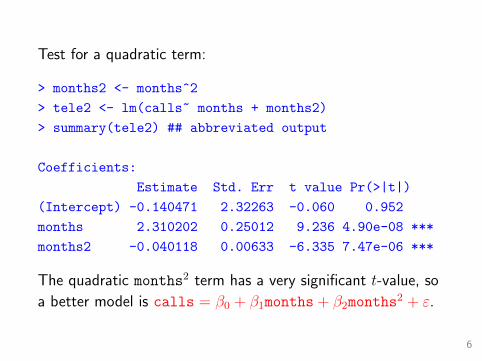
Test for a quadratic term:
> months2 <- months^2
> tele2 <- lm(calls~ months + months2)
> summary(tele2) ## abbreviated output
Coefficients:
Estimate Std. Err t value Pr(>|t|)
(Intercept) -0.140471 2.32263 -0.060 0.952
months 2.310202 0.25012 9.236 4.90e-08 ***
months2 -0.040118 0.00633 -6.335 7.47e-06 ***
The quadratic months2 term has a very significant t-value, so
a better model is calls = β0 + β1months + β2months2 + ε.
6
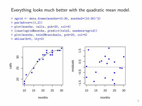
Everything looks much better with the quadratic mean model.
> xgrid <- data.frame(months=10:30, months2=(10:30)^2)
> par(mfrow=c(1,2))
> plot(months, calls, pch=20, col=4)
> lines(xgrid$months, predict(tele2, newdata=xgrid))
> plot(months, tele2$residuals, pch=20, col=4)
> abline(h=0, lty=2)
●
●
●
●
●
●
● ●
● ●
●
●
●
●●
●
●
● ●
●
10 15 20 25 30
2025
30
months
calls
●
●
●
●
●
●●
●
●
●
●
●
●
●●
●
●
● ●
●
10 15 20 25 30
−1.
5−
0.5
0.5
1.5
months
resi
dual
s
7

A few words of caution
We can always add higher powers (cubic, etc.) if necessary.
I If you add a higher order term, the lower order term is
kept regardless of its individual t-stat.(see handout on website)
Be very careful about predicting outside the data range;
I the curve may do unintended things beyond the data.
Watch out for over-fitting.
I You can get a “perfect” fit with enough polynomial terms,
I but that doesn’t mean it will be any good for prediction
or understanding.
8
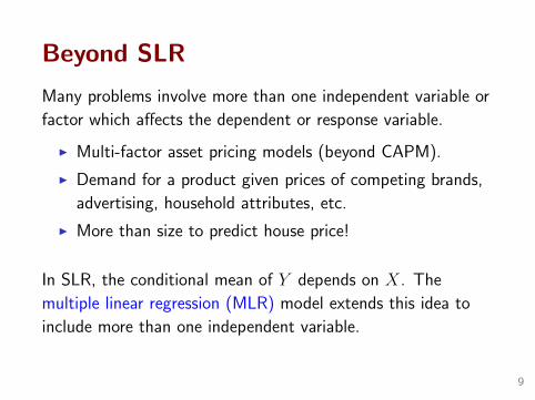
Beyond SLR
Many problems involve more than one independent variable or
factor which affects the dependent or response variable.
I Multi-factor asset pricing models (beyond CAPM).
I Demand for a product given prices of competing brands,
advertising, household attributes, etc.
I More than size to predict house price!
In SLR, the conditional mean of Y depends on X. The
multiple linear regression (MLR) model extends this idea to
include more than one independent variable.
9
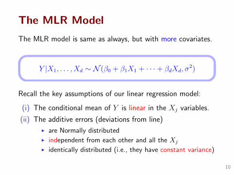
The MLR Model
The MLR model is same as always, but with more covariates.
Y |X1, . . . , Xd ∼ N (β0 + β1X1 + · · ·+ βdXd, σ2)
Recall the key assumptions of our linear regression model:
(i) The conditional mean of Y is linear in the Xj variables.
(ii) The additive errors (deviations from line)
I are Normally distributedI independent from each other and all the Xj
I identically distributed (i.e., they have constant variance)
10
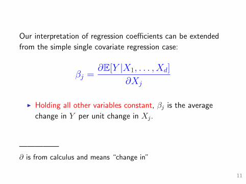
Our interpretation of regression coefficients can be extended
from the simple single covariate regression case:
βj =∂E[Y |X1, . . . , Xd]
∂Xj
I Holding all other variables constant, βj is the average
change in Y per unit change in Xj.
—————
∂ is from calculus and means “change in”
11
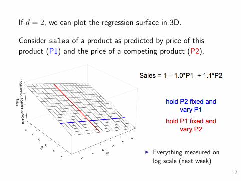
If d = 2, we can plot the regression surface in 3D.
Consider sales of a product as predicted by price of this
product (P1) and the price of a competing product (P2).
I Everything measured on
log scale (next week)
12
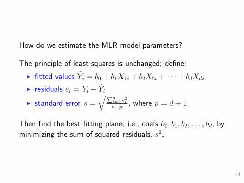
How do we estimate the MLR model parameters?
The principle of least squares is unchanged; define:
I fitted values Yi = b0 + b1X1i + b2X2i + · · ·+ bdXdi
I residuals ei = Yi − YiI standard error s =
√∑ni=1 e
2i
n−p , where p = d+ 1.
Then find the best fitting plane, i.e., coefs b0, b1, b2, . . . , bd, by
minimizing the sum of squared residuals, s2.
13
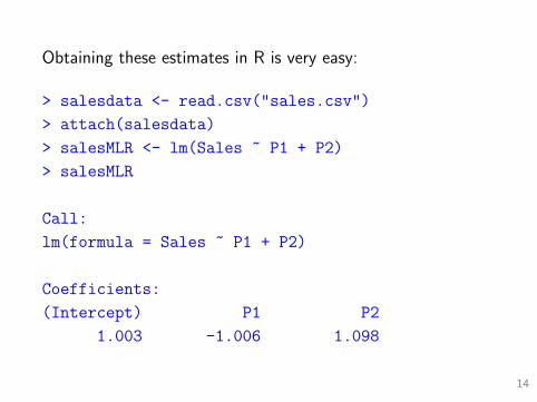
Obtaining these estimates in R is very easy:
> salesdata <- read.csv("sales.csv")
> attach(salesdata)
> salesMLR <- lm(Sales ~ P1 + P2)
> salesMLR
Call:
lm(formula = Sales ~ P1 + P2)
Coefficients:
(Intercept) P1 P2
1.003 -1.006 1.098
14
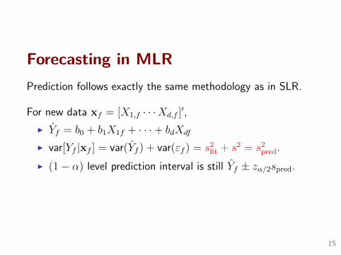
Forecasting in MLR
Prediction follows exactly the same methodology as in SLR.
For new data xf = [X1,f · · ·Xd,f ]′,
I Yf = b0 + b1X1f + · · ·+ bdXdf
I var[Yf |xf ] = var(Yf ) + var(εf ) = s2fit + s2 = s2
pred.
I (1− α) level prediction interval is still Yf ± zα/2spred.
15
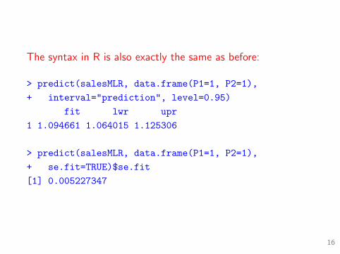
The syntax in R is also exactly the same as before:
> predict(salesMLR, data.frame(P1=1, P2=1),
+ interval="prediction", level=0.95)
fit lwr upr
1 1.094661 1.064015 1.125306
> predict(salesMLR, data.frame(P1=1, P2=1),
+ se.fit=TRUE)$se.fit
[1] 0.005227347
16
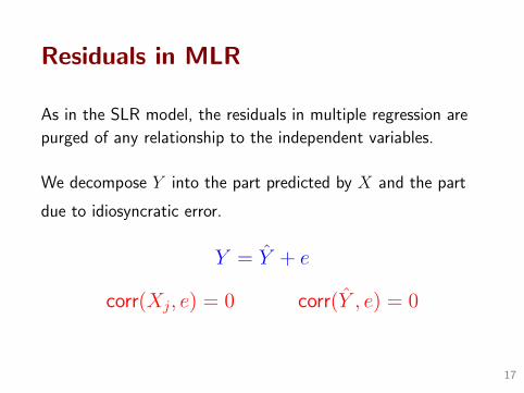
Residuals in MLR
As in the SLR model, the residuals in multiple regression are
purged of any relationship to the independent variables.
We decompose Y into the part predicted by X and the part
due to idiosyncratic error.
Y = Y + e
corr(Xj, e) = 0 corr(Y , e) = 0
17
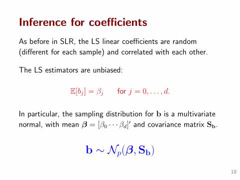
Inference for coefficients
As before in SLR, the LS linear coefficients are random
(different for each sample) and correlated with each other.
The LS estimators are unbiased:
E[bj] = βj for j = 0, . . . , d.
In particular, the sampling distribution for b is a multivariate
normal, with mean β = [β0 · · · βd]′ and covariance matrix Sb.
b ∼ Np(β,Sb)
18
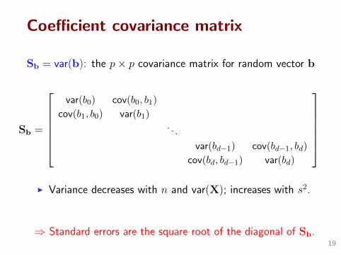
Coefficient covariance matrix
Sb = var(b): the p× p covariance matrix for random vector b
Sb =
var(b0) cov(b0, b1)
cov(b1, b0) var(b1). . .
var(bd−1) cov(bd−1, bd)
cov(bd, bd−1) var(bd)
I Variance decreases with n and var(X); increases with s2.
⇒ Standard errors are the square root of the diagonal of Sb.19
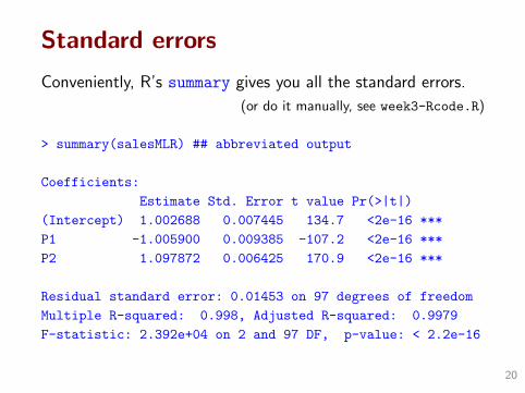
Standard errors
Conveniently, R’s summary gives you all the standard errors.
(or do it manually, see week3-Rcode.R)
> summary(salesMLR) ## abbreviated output
Coefficients:
Estimate Std. Error t value Pr(>|t|)
(Intercept) 1.002688 0.007445 134.7 <2e-16 ***
P1 -1.005900 0.009385 -107.2 <2e-16 ***
P2 1.097872 0.006425 170.9 <2e-16 ***
Residual standard error: 0.01453 on 97 degrees of freedom
Multiple R-squared: 0.998, Adjusted R-squared: 0.9979
F-statistic: 2.392e+04 on 2 and 97 DF, p-value: < 2.2e-16
20
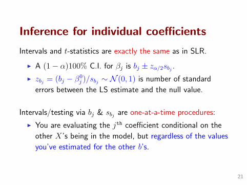
Inference for individual coefficients
Intervals and t-statistics are exactly the same as in SLR.
I A (1− α)100% C.I. for βj is bj ± zα/2sbj .
I zbj = (bj − β0j )/sbj ∼ N (0, 1) is number of standard
errors between the LS estimate and the null value.
Intervals/testing via bj & sbj are one-at-a-time procedures:
I You are evaluating the jth coefficient conditional on the
other X’s being in the model, but regardless of the values
you’ve estimated for the other b’s.
21
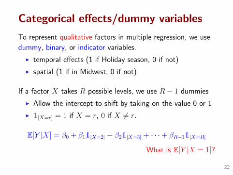
Categorical effects/dummy variables
To represent qualitative factors in multiple regression, we use
dummy, binary, or indicator variables.
I temporal effects (1 if Holiday season, 0 if not)
I spatial (1 if in Midwest, 0 if not)
If a factor X takes R possible levels, we use R− 1 dummies
I Allow the intercept to shift by taking on the value 0 or 1
I 1[X=r] = 1 if X = r, 0 if X 6= r.
E[Y |X] = β0 + β11[X=2] + β21[X=3] + · · ·+ βR−11[X=R]
What is E[Y |X = 1]?
22
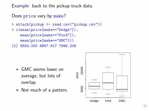
Example: back to the pickup truck data.
Does price vary by make?
> attach(pickup <- read.csv("pickup.csv"))
> c(mean(price[make=="Dodge"]),
mean(price[make=="Ford"]),
mean(price[make=="GMC"]))
[1] 6554.200 8867.917 7996.208
I GMC seems lower on
average, but lots of
overlap.
I Not much of a pattern.
Dodge Ford GMC
5000
1500
0
pric
e
23
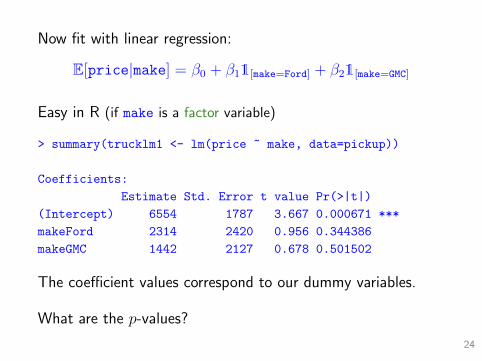
Now fit with linear regression:
E[price|make] = β0 + β11[make=Ford] + β21[make=GMC]
Easy in R (if make is a factor variable)
> summary(trucklm1 <- lm(price ~ make, data=pickup))
Coefficients:
Estimate Std. Error t value Pr(>|t|)
(Intercept) 6554 1787 3.667 0.000671 ***
makeFord 2314 2420 0.956 0.344386
makeGMC 1442 2127 0.678 0.501502
The coefficient values correspond to our dummy variables.
What are the p-values?
24
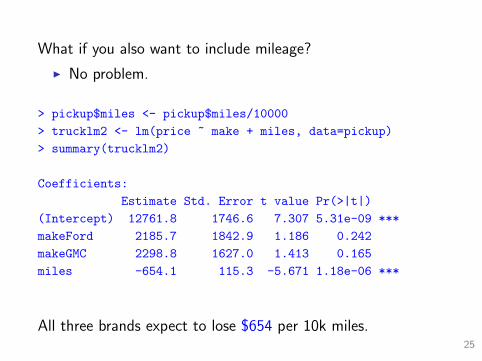
What if you also want to include mileage?
I No problem.
> pickup$miles <- pickup$miles/10000
> trucklm2 <- lm(price ~ make + miles, data=pickup)
> summary(trucklm2)
Coefficients:
Estimate Std. Error t value Pr(>|t|)
(Intercept) 12761.8 1746.6 7.307 5.31e-09 ***
makeFord 2185.7 1842.9 1.186 0.242
makeGMC 2298.8 1627.0 1.413 0.165
miles -654.1 115.3 -5.671 1.18e-06 ***
All three brands expect to lose $654 per 10k miles.25
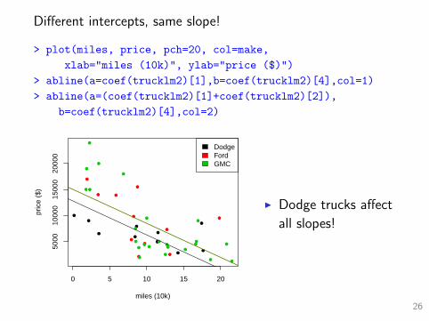
Different intercepts, same slope!
> plot(miles, price, pch=20, col=make,
xlab="miles (10k)", ylab="price ($)")
> abline(a=coef(trucklm2)[1],b=coef(trucklm2)[4],col=1)
> abline(a=(coef(trucklm2)[1]+coef(trucklm2)[2]),
b=coef(trucklm2)[4],col=2)
●
●
●
●
●
●
●
●
●
●
●
●
●
●
●
●
●
●
●
●●
●
●
●
●
●
●
●
●●
●
●
●
●
●
●
●
●
●●
●
●
●
●●
●
0 5 10 15 20
5000
1000
015
000
2000
0
miles (10k)
pric
e ($
)
DodgeFordGMC
I Dodge trucks affect
all slopes!
26

Variable interaction
So far we have considered the impact of each independent
variable in a additive way.
We can extend this notion and include interaction effects
through multiplicative terms.
Yi = β0 + β1X1i + β2X2i + β3(X1iX2i) + · · ·+ εi
∂E[Y |X1, X2]
∂X1= β1 + β3X2
27

Interactions with dummy variables
Dummy variables separate out categories
I Different intercept for each category
Interactions with dummies separate out trends
I Different slope for each category
Yi = β0 + β11{X1i=1} + β2X2i + β3(1{X1i=1}X2i) + · · ·+ εi
∂E[Y |X1 = 0, X2]
∂X2
= β2∂E[Y |X1 = 1, X2]
∂X2
= β2 + β3
28
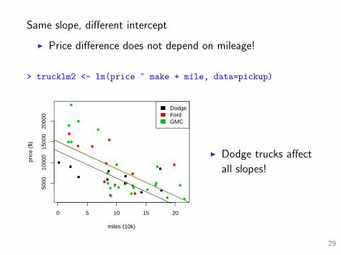
Same slope, different intercept
I Price difference does not depend on mileage!
> trucklm2 <- lm(price ~ make + mile, data=pickup)
●
●
●
●
●
●
●
●
●
●
●
●
●
●
●
●
●
●
●
●●
●
●
●
●
●
●
●
●●
●
●
●
●
●
●
●
●
●●
●
●
●
●●
●
0 5 10 15 20
5000
1000
015
000
2000
0
miles (10k)
pric
e ($
)
DodgeFordGMC
I Dodge trucks affect
all slopes!
29
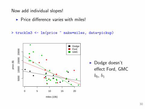
Now add individual slopes!
I Price difference varies with miles!
> trucklm3 <- lm(price ~ make*miles, data=pickup)
●
●
●
●
●
●
●
●
●
●
●
●
●
●
●
●
●
●
●
●●
●
●
●
●
●
●
●
●●
●
●
●
●
●
●
●
●
●●
●
●
●
●●
●
0 5 10 15 20
5000
1000
015
000
2000
0
miles (10k)
pric
e ($
)
DodgeFordGMC
I Dodge doesn’t
effect Ford, GMC
b0, b1
30
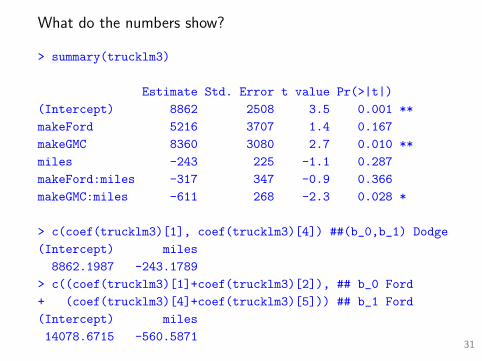
What do the numbers show?
> summary(trucklm3)
Estimate Std. Error t value Pr(>|t|)
(Intercept) 8862 2508 3.5 0.001 **
makeFord 5216 3707 1.4 0.167
makeGMC 8360 3080 2.7 0.010 **
miles -243 225 -1.1 0.287
makeFord:miles -317 347 -0.9 0.366
makeGMC:miles -611 268 -2.3 0.028 *
> c(coef(trucklm3)[1], coef(trucklm3)[4]) ##(b_0,b_1) Dodge
(Intercept) miles
8862.1987 -243.1789
> c((coef(trucklm3)[1]+coef(trucklm3)[2]), ## b_0 Ford
+ (coef(trucklm3)[4]+coef(trucklm3)[5])) ## b_1 Ford
(Intercept) miles
14078.6715 -560.587131
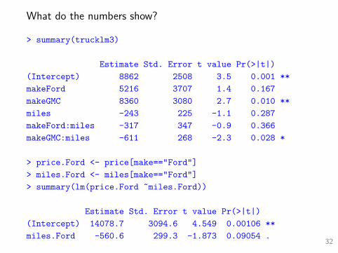
What do the numbers show?
> summary(trucklm3)
Estimate Std. Error t value Pr(>|t|)
(Intercept) 8862 2508 3.5 0.001 **
makeFord 5216 3707 1.4 0.167
makeGMC 8360 3080 2.7 0.010 **
miles -243 225 -1.1 0.287
makeFord:miles -317 347 -0.9 0.366
makeGMC:miles -611 268 -2.3 0.028 *
> price.Ford <- price[make=="Ford"]
> miles.Ford <- miles[make=="Ford"]
> summary(lm(price.Ford ~miles.Ford))
Estimate Std. Error t value Pr(>|t|)
(Intercept) 14078.7 3094.6 4.549 0.00106 **
miles.Ford -560.6 299.3 -1.873 0.09054 .32
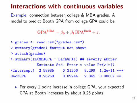
Interactions with continuous variablesExample: connection between college & MBA grades. A
model to predict Booth GPA from college GPA could be
GPAMBA = β0 + β1GPABach + ε.
> grades <- read.csv("grades.csv")
> summary(grades) #output not shown
> attach(grades)
> summary(lm(MBAGPA ~ BachGPA)) ## severly abbrev.
Estimate Std. Error t value Pr(>|t|)
(Intercept) 2.58985 0.31206 8.299 1.2e-11 ***
BachGPA 0.26269 0.09244 2.842 0.00607 **
I For every 1 point increase in college GPA, your expected
GPA at Booth increases by about 0.26 points.33
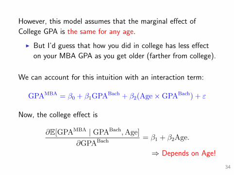
However, this model assumes that the marginal effect of
College GPA is the same for any age.
I But I’d guess that how you did in college has less effect
on your MBA GPA as you get older (farther from college).
We can account for this intuition with an interaction term:
GPAMBA = β0 + β1GPABach + β2(Age×GPABach) + ε
Now, the college effect is
∂E[GPAMBA | GPABach,Age]
∂GPABach= β1 + β2Age.
⇒ Depends on Age!
34
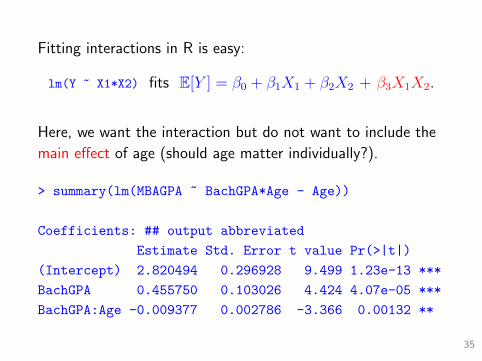
Fitting interactions in R is easy:
lm(Y ~ X1*X2) fits E[Y ] = β0 + β1X1 + β2X2 + β3X1X2.
Here, we want the interaction but do not want to include the
main effect of age (should age matter individually?).
> summary(lm(MBAGPA ~ BachGPA*Age - Age))
Coefficients: ## output abbreviated
Estimate Std. Error t value Pr(>|t|)
(Intercept) 2.820494 0.296928 9.499 1.23e-13 ***
BachGPA 0.455750 0.103026 4.424 4.07e-05 ***
BachGPA:Age -0.009377 0.002786 -3.366 0.00132 **
35
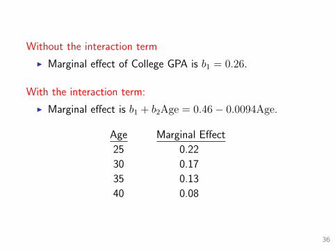
Without the interaction term
I Marginal effect of College GPA is b1 = 0.26.
With the interaction term:
I Marginal effect is b1 + b2Age = 0.46− 0.0094Age.
Age Marginal Effect
25 0.22
30 0.17
35 0.13
40 0.08
36
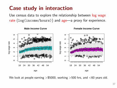
Case study in interactionUse census data to explore the relationship between log wage
rate (log(income/hours)) and age—a proxy for experience.
●●
●●
●●
●
●●●
●
●
●
●
●●●
●●
●●●
●●
●
●
●
●
●
●
●●●●
●●
●
●●
●●●
●
●
●
●
●
●●●●●
●
●
●
●
●●●
●
●
●●
●●
●
●
●
●
●
●●
●●
●
●
●
●
●
●●●
●
●
●
●
●
●
●●
●
●
●●
●
●
●
●
●
●
●●●
●●
●●●
●
●
●
●
●
●
●●
●●
●●
●
●●●●●●
●●●
●●●●●●●●
●
●●
●
●
●●
●●
●●
●
●●
●
●●
●
●
●
●●
●
●
●
●
●
●
●
●
●●●
●
●
●●
●●
●●●
●
●
●●●
●●●●●
●●
●●
●
●
●
●
●
●
●●
●
●
●
●
●●●
●
●●●●●
●
●
●
●
●●
●●●
●
●●
●
●●
●
●●●●
●
●●●●●
●●●
●
●
●
●●●●●●●
●
●
●
●
●
●●●●
●●
●●●●●
●●●
●●
●
●●●
●
●●●
●●
●
●
●
●
●●
●●
●
●●
●●
●
●●●●
●
●●
●●●●●●●●●
●●●●
●
●●
●●
●●
●
●
●
●●●
●●●
●
●●
●●●
●●
●
●●●
●
●●●●●●
●
●●●●●●●●
●
●●●●●
●
●●●●
●
●●
●
●●●●
●
●●●
●
●
●
●●●
●
18 24 30 36 42 48 54
01
23
45
6
Male Income Curve
age
log
wag
e ra
te
●
●●
●
●●
●
●●
●
●●
●●●●
●●●●
●
●
●●
●●
●
●●
●●
●●
●
●
●
●●
●
●●●●
●●
●
●●
●●
●
●●
●
●
●
●
●
●●●
●
●
●
●●
●
●
●
●
●
●
●
●
●
●●
●●●
●●
●
●
●●
●●●
●
●
●
●
●
●
●●
●
●
●
●
●
●
●●●
●
●●
●●
●
●●
●●
●
●●
●●●
●
●
●●
●
●●
●
●●●
●
●
●
●
●
●
●●
●
●
●
●●●
●
●●●
●
18 24 30 36 42 48 540
12
34
56
Female Income Curve
age
log
wag
e ra
te
We look at people earning >$5000, working >500 hrs, and <60 years old.
37
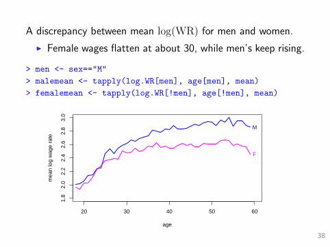
A discrepancy between mean log(WR) for men and women.
I Female wages flatten at about 30, while men’s keep rising.
> men <- sex=="M"
> malemean <- tapply(log.WR[men], age[men], mean)
> femalemean <- tapply(log.WR[!men], age[!men], mean)
20 30 40 50 60
1.8
2.0
2.2
2.4
2.6
2.8
3.0
age
mea
n lo
g w
age
rate
M
F
38
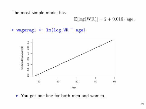
The most simple model has
E[log(WR)] = 2 + 0.016 · age.
> wagereg1 <- lm(log.WR ~ age)
20 30 40 50 60
2.3
2.4
2.5
2.6
2.7
2.8
2.9
age
pred
icte
d lo
g w
ager
ate
I You get one line for both men and women.
39
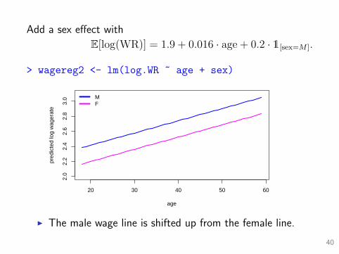
Add a sex effect with
E[log(WR)] = 1.9 + 0.016 · age + 0.2 · 1[sex=M ].
> wagereg2 <- lm(log.WR ~ age + sex)
20 30 40 50 60
2.0
2.2
2.4
2.6
2.8
3.0
age
pred
icte
d lo
g w
ager
ate
MF
I The male wage line is shifted up from the female line.
40
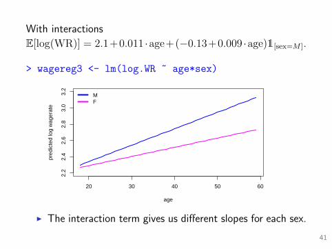
With interactions
E[log(WR)] = 2.1+0.011 ·age+(−0.13+0.009 ·age)1[sex=M ].
> wagereg3 <- lm(log.WR ~ age*sex)
20 30 40 50 60
2.2
2.4
2.6
2.8
3.0
3.2
age
pred
icte
d lo
g w
ager
ate
MF
I The interaction term gives us different slopes for each sex.
41
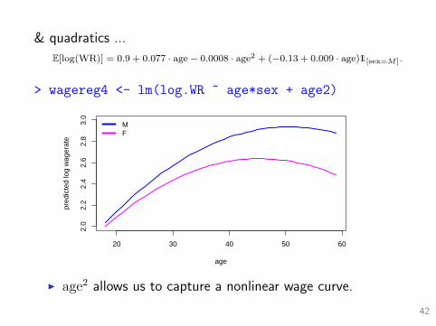
& quadratics ...
E[log(WR)] = 0.9 + 0.077 · age− 0.0008 · age2 + (−0.13 + 0.009 · age)1[sex=M ].
> wagereg4 <- lm(log.WR ~ age*sex + age2)
20 30 40 50 60
2.0
2.2
2.4
2.6
2.8
3.0
age
pred
icte
d lo
g w
ager
ate
MF
I age2 allows us to capture a nonlinear wage curve.
42
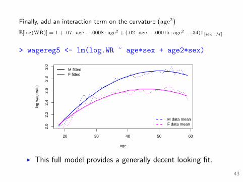
Finally, add an interaction term on the curvature (age2)
E[log(WR)] = 1 + .07 · age− .0008 · age2 + (.02 · age− .00015 · age2 − .34)1[sex=M ].
> wagereg5 <- lm(log.WR ~ age*sex + age2*sex)
20 30 40 50 60
2.0
2.2
2.4
2.6
2.8
3.0
age
log
wag
erat
e
M fittedF fitted
M data meanF data mean
I This full model provides a generally decent looking fit.
43

We could also consider a model that has an interaction
between age and edu.
I reg <- lm(log.WR ~ edu*age)
Maybe we don’t need the age main effect?
I reg <- lm(log.WR ~ edu*age - age)
Or perhaps all of the extra edu effects are unnecessary?
I reg <- lm(log.WR ~ edu*age - edu)
44
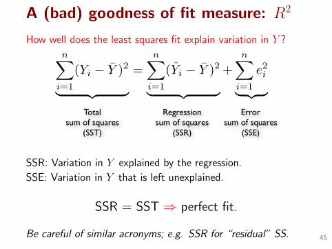
A (bad) goodness of fit measure: R2
How well does the least squares fit explain variation in Y ?
nX
i=1
(Yi � Y )2
| {z }=
nX
i=1
(Yi � Y )2
| {z }+
nX
i=1
e2i
| {z }Total
sum of squares(SST)
Regression sum of squares
(SSR)
Error sum of squares
(SSE)
SSR: Variation in Y explained by the regression.
SSE: Variation in Y that is left unexplained.
SSR = SST ⇒ perfect fit.
Be careful of similar acronyms; e.g. SSR for “residual” SS. 45
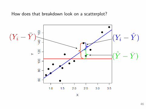
How does that breakdown look on a scatterplot?
Week II. Slide 23Applied Regression Analysis – Fall 2008 Matt Taddy
Decomposing the Variance – The ANOVA Table
46
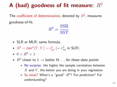
A (bad) goodness of fit measure: R2
The coefficient of determination, denoted by R2, measures
goodness-of-fit:
R2 =SSR
SST
I SLR or MLR: same formula.
I R2 = corr2(Y , Y ) = r2yy (= r2
xy in SLR)
I 0 < R2 < 1.
I R2 closer to 1 → better fit . . . for these data points
I No surprise: the higher the sample correlation between
X and Y , the better you are doing in your regression.I So what? What’s a “good” R2? For prediction? For
understanding?47
Adjusted R2
This is the reason some people like to look at adjusted R2
R2a = 1− s2/s2
y
Since s2/s2y is a ratio of variance estimates, R2
a will not
necessarily increase when new variables are added.
Unfortunately, R2a is useless!
I The problem is that there is no theory for inference about
R2a, so we will not be able to tell “how big is big”.
48
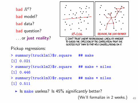
bad R2?
bad model?
bad data?
bad question?
. . . or just reality?
Pickup regressions:
> summary(trucklm1)$r.square ## make
[1] 0.021
> summary(trucklm2)$r.square ## make + miles
[1] 0.446
> summary(trucklm3)$r.square ## make * miles
[1] 0.511
I Is make useless? Is 45% significantly better?
(We’ll formalize in 2 weeks.) 49
Up next: choosing a regression model
What’s a good regression?
Next week:
I Problems and diagnostics
I Some fixes
Week 5:
I MLR for causation
I Testing for fit
Week 7
I BIC, model choice algorithms
I Big p problems (data mining)50
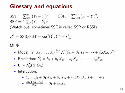
Glossary and equations
SST =∑n
i=1(Yi − Y )2, SSR =∑n
i=1(Yi − Y )2,
SSE =∑n
i=1(Yi − Yi)2
(Watch out: sometimes SSE is called SSR or RSS!)
R2 = SSR/SST = cor2(Y , Y ) = r2yy
MLR:
I Model: Y |X1, . . . , Xdind∼ N (β0 + β1X1 + · · ·+ βdXd, σ
2)
I Prediction: Yi = b0 + b1X1i + b2X2i + · · ·+ bdXdi
I b ∼ Np(β,Sb)
I Interaction:
I Yi = β0 + β1X1i + β2X2i + β3(X1iX2i) + . . .+ ε
I∂E[Y |X1,X2]
∂X1= β1 + β3X2
51


![Applied Nonparametric Regression [Hardle]](https://img.pdfslide.us/doc/110x75/551eb84d497959cf398b4b76/applied-nonparametric-regression-hardle.jpg)


![[Bruderl] Applied Regression Analysis Using Stata](https://img.pdfslide.us/doc/110x75/55cf96a7550346d0338ce88d/bruderl-applied-regression-analysis-using-stata.jpg)

