8/2/2019 BUS161 Topic 4 2012

http://slidepdf.com/reader/full/bus161-topic-4-2012 1/26

8/2/2019 BUS161 Topic 4 2012

http://slidepdf.com/reader/full/bus161-topic-4-2012 2/26

Murdoch University, Perth, Western Australia, 2012; Pearson Australia 2012.

2

Technology: An economic definition

Technology: The processes a firm usesto turn inputs into outputs of goods andservices.

Technological change: A change in theability of a firm to produce a different levelof output with a given quantity of inputs.

8/2/2019 BUS161 Topic 4 2012

http://slidepdf.com/reader/full/bus161-topic-4-2012 3/26

Murdoch University, Perth, Western Australia, 2012; Pearson Australia 2012.

3

The short run and the long run

Short run: The period of time duringwhich at least one of a firm’s inputs is

fixed.

Long run: A period of time long enoughto allow a firm to vary all of its inputs, to

adopt new technology, and to increase ordecrease the size of its physical plant.

8/2/2019 BUS161 Topic 4 2012

http://slidepdf.com/reader/full/bus161-topic-4-2012 4/26

Murdoch University, Perth, Western Australia, 2012; Pearson Australia 2012.

4

A summary of costs 

Costs and revenue are analysed at the‘margin’. 

Marginal Cost (MC) = the change in thefirm’s total cost from producing one more

unit or a good or service.

Change in TC

Change in Q 

8/2/2019 BUS161 Topic 4 2012

http://slidepdf.com/reader/full/bus161-topic-4-2012 5/26

Murdoch University, Perth, Western Australia, 2012; Pearson Australia 2012.

5

Total Cost (TC) = The costs of all the inputsa firm uses in production, including totalvariable costs and total fixed costs.

Average Total Cost (ATC) = TC/Q

Variable Costs (VC) are costs that changewith the volume of output produced.

Examples: wages, raw materials

Average variable cost (AVC): Variablecost divided by the quantity of outputproduced.

A summary of costs 

8/2/2019 BUS161 Topic 4 2012

http://slidepdf.com/reader/full/bus161-topic-4-2012 6/26

Murdoch University, Perth, Western Australia, 2012; Pearson Australia 2012.

6

Fixed Costs are costs that remain constantas the level of output changes.

Examples: rent, land rates, interestrepayments

Average fixed cost: Fixed cost divided bythe quantity of output produced.

A summary of costs 

8/2/2019 BUS161 Topic 4 2012

http://slidepdf.com/reader/full/bus161-topic-4-2012 7/26 Murdoch University, Perth, Western Australia, 2012; Pearson Australia 2012.

7

Implicit costs and explicit costs

Explicit cost: A cost that involvesspending money. (Accounting costs)

Implicit cost: A non-monetary opportunitycost.

Economic costs include explicit andimplicit costs.

8/2/2019 BUS161 Topic 4 2012

http://slidepdf.com/reader/full/bus161-topic-4-2012 8/26

 

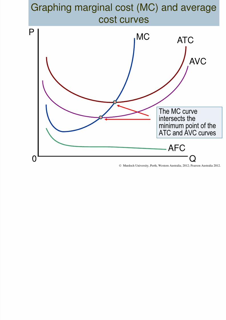
ATC MC 

P 

Q 0 

Graphing marginal cost (MC) and averagecost curves

The MC curve

intersects theminimum point of the ATC and AVC curves

AVC 

AFC 

Murdoch University, Perth, Western Australia, 2012; Pearson Australia 2012.

8/2/2019 BUS161 Topic 4 2012

http://slidepdf.com/reader/full/bus161-topic-4-2012 9/26 Murdoch University, Perth, Western Australia, 2012; Pearson Australia 2012.

9

The marginal product of labour

Marginal product of labour: Theadditional output a firm produces as aresult of hiring one more worker.

Law of diminishing returns: Theprinciple that, at some point, adding moreof a variable input, such as labour, to thesame amount of a fixed input, such as

capital, will cause the marginal product ofthe variable input to decline.

8/2/2019 BUS161 Topic 4 2012

http://slidepdf.com/reader/full/bus161-topic-4-2012 10/26 Murdoch University, Perth, Western Australia, 2012; Pearson Australia 2012.

10

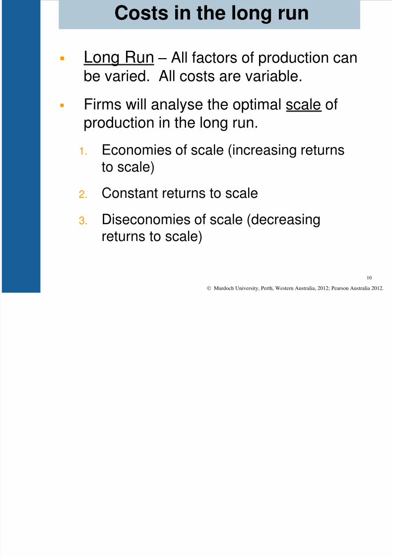
Costs in the long run

Long Run  – All factors of production can

be varied. All costs are variable.

Firms will analyse the optimal scale ofproduction in the long run.

1. Economies of scale (increasing returnsto scale)

2. Constant returns to scale

3. Diseconomies of scale (decreasingreturns to scale)

8/2/2019 BUS161 Topic 4 2012

http://slidepdf.com/reader/full/bus161-topic-4-2012 11/26 Murdoch University, Perth, Western Australia, 2012; Pearson Australia 2012.

11

Long-run average cost curve: A curveshowing the lowest cost at which the firmis able to produce a given quantity ofoutput in the long run, when no inputsare fixed.

1. Economies of scale: Exist when afirm’s long-run average costs fall as it

increases its scale of production and thequantity of output it produces.

Costs in the long run

8/2/2019 BUS161 Topic 4 2012

http://slidepdf.com/reader/full/bus161-topic-4-2012 12/26 Murdoch University, Perth, Western Australia, 2012; Pearson Australia 2012.

12

Minimum efficient scale: The level ofoutput at which all economies of scalehave been exhausted.

It is the minimum point on the long run

average cost curve.

Costs in the long run

8/2/2019 BUS161 Topic 4 2012

http://slidepdf.com/reader/full/bus161-topic-4-2012 13/26 Murdoch University, Perth, Western Australia, 2012; Pearson Australia 2012.

13

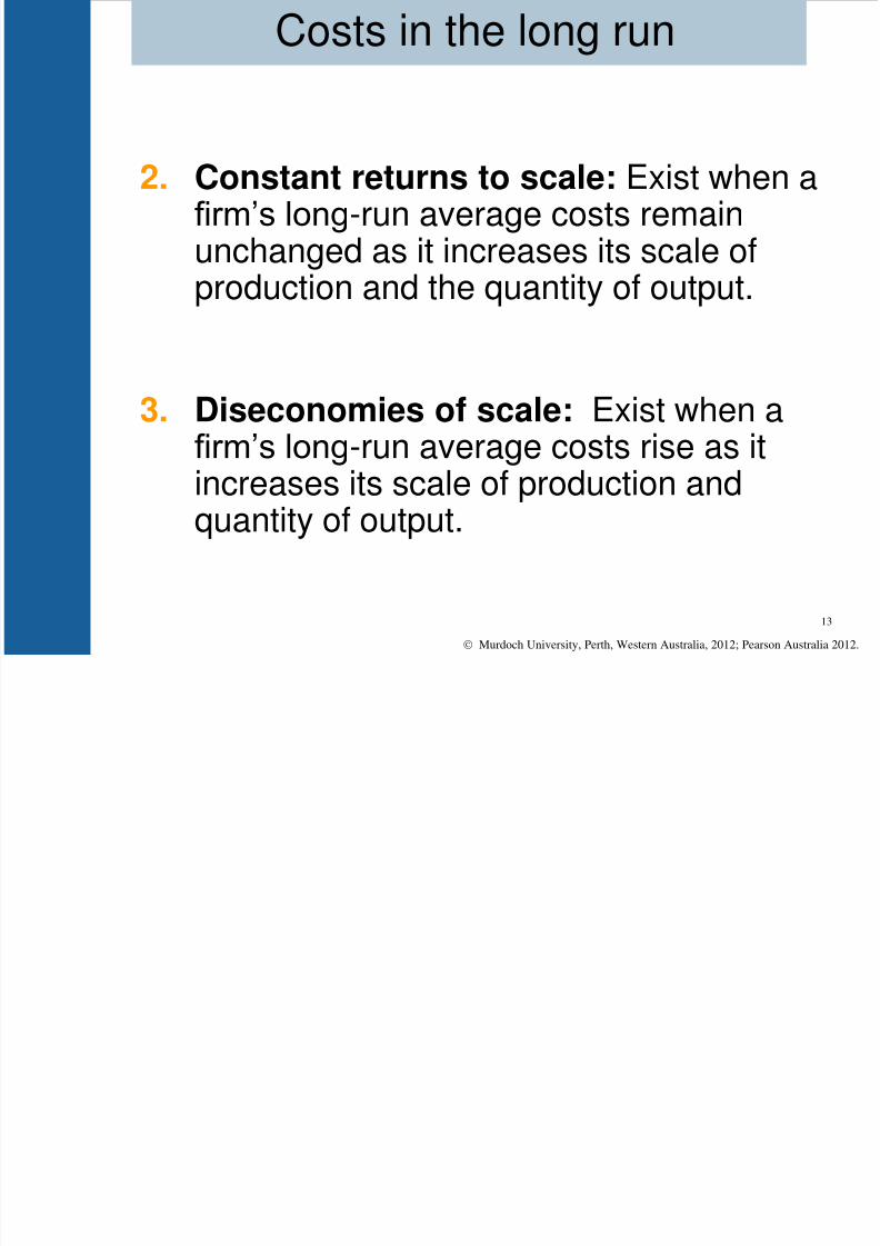
2. Constant returns to scale: Exist when afirm’s long-run average costs remainunchanged as it increases its scale ofproduction and the quantity of output.

3. Diseconomies of scale: Exist when a

firm’s long-run average costs rise as itincreases its scale of production andquantity of output.

Costs in the long run

8/2/2019 BUS161 Topic 4 2012

http://slidepdf.com/reader/full/bus161-topic-4-2012 14/26

Economies of scale

Economies of scale occur when all inputs are

increased by x% and output increase by morethan x%.

LAC

Q0 A

Long runaverage cost

(LAC)Economies ofscale

Minimumefficientscale

Murdoch University, Perth, Western Australia, 2012; Pearson Australia 2012.

8/2/2019 BUS161 Topic 4 2012

http://slidepdf.com/reader/full/bus161-topic-4-2012 15/26 Murdoch University, Perth, Western Australia, 2012; Pearson Australia 2012.

15

Sources of economies of scale

1. Specialisation labour

machinery

2. Bulk buying leading to cheaper inputs

3. Spreading overhead costs

4. Financial economies eg: negotiating lower interest rates

8/2/2019 BUS161 Topic 4 2012

http://slidepdf.com/reader/full/bus161-topic-4-2012 16/26 Murdoch University, Perth, Western Australia, 2012; Pearson Australia 2012.

16

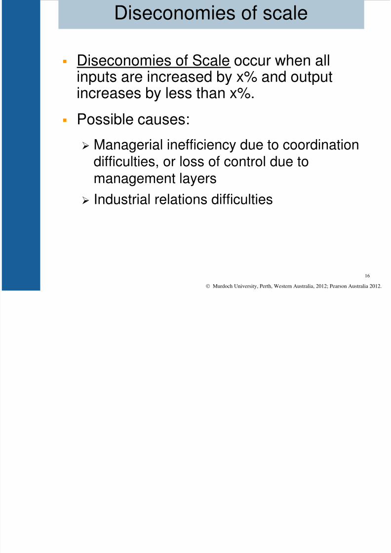
Diseconomies of scale

Diseconomies of Scale occur when allinputs are increased by x% and outputincreases by less than x%.

Possible causes: 

Managerial inefficiency due to coordinationdifficulties, or loss of control due tomanagement layers

Industrial relations difficulties

8/2/2019 BUS161 Topic 4 2012

http://slidepdf.com/reader/full/bus161-topic-4-2012 17/26

Diseconomies of scale

LAC

Q0

A

Long run averagecost (LAC)

Diseconomiesof scale

Murdoch University, Perth, Western Australia, 2012; Pearson Australia 2012.

8/2/2019 BUS161 Topic 4 2012

http://slidepdf.com/reader/full/bus161-topic-4-2012 18/26 Murdoch University, Perth, Western Australia, 2012; Pearson Australia 2012.

18

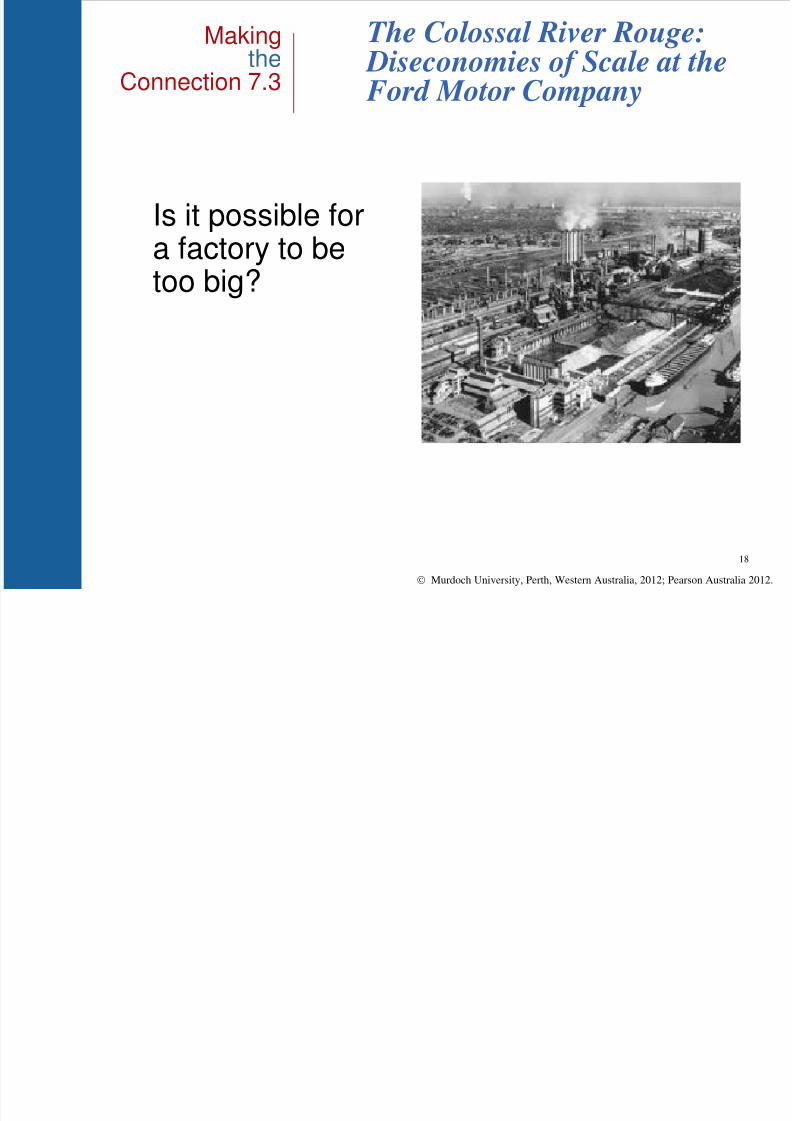
The Colossal River Rouge: Diseconomies of Scale at the Ford Motor Company

Is it possible fora factory to be

too big?

Making the

Connection 7.3

C t t t t l

8/2/2019 BUS161 Topic 4 2012

http://slidepdf.com/reader/full/bus161-topic-4-2012 19/26

Constant returns to scale

Constant returns to scale occur beyond point A.

Point A is the ‘minimum efficient scale’. 

A

LAC

Q

0

LAC

Murdoch University, Perth, Western Australia, 2012; Pearson Australia 2012.

8/2/2019 BUS161 Topic 4 2012

http://slidepdf.com/reader/full/bus161-topic-4-2012 20/26 Murdoch University, Perth, Western Australia, 2012; Pearson Australia 2012.

20

Next

Topic 5

Market Structures, Competitionand Economic Efficiency

8/2/2019 BUS161 Topic 4 2012

http://slidepdf.com/reader/full/bus161-topic-4-2012 21/26 Murdoch University, Perth, Western Australia, 2012; Pearson Australia 2012.

21

Check Your Knowledge

Q1. Which of the following aresometimes called accounting costs?

a. Economic costs.

b. Implicit costs.

c. Explicit costs.d. Total variable costs.

8/2/2019 BUS161 Topic 4 2012

http://slidepdf.com/reader/full/bus161-topic-4-2012 22/26 Murdoch University, Perth, Western Australia, 2012; Pearson Australia 2012.

22

Check Your Knowledge

Q1. Which of the following aresometimes called accounting costs?

a. Economic costs.

b. Implicit costs.

c.Explicit costs.

d. Total variable costs.

8/2/2019 BUS161 Topic 4 2012

http://slidepdf.com/reader/full/bus161-topic-4-2012 23/26 Murdoch University, Perth, Western Australia, 2012; Pearson Australia 2012.

23

Q2. When does the law of diminishing

returns apply?

a. When there are diseconomies of scale.b. In the short run only.

c. In the long run only.

d. In both the short run and the long run.

Check Your Knowledge

8/2/2019 BUS161 Topic 4 2012

http://slidepdf.com/reader/full/bus161-topic-4-2012 24/26

Murdoch University, Perth, Western Australia, 2012; Pearson Australia 2012.

24

Q2. When does the law of diminishing

returns apply?

a. When there are diseconomies of scale.b. In the short run only.

c. In the long run only.

d. In both the short run and the long run.

Check Your Knowledge

8/2/2019 BUS161 Topic 4 2012

http://slidepdf.com/reader/full/bus161-topic-4-2012 25/26

Murdoch University, Perth, Western Australia, 2012; Pearson Australia 2012.

25

Q3.  When a firm increases all of itsinputs by 5 per cent and its outputincreases by 4 per cent, it is

experiencing:a. Diseconomies of scale.

b. Economies of scale.

c. Diminishing returns.

d. Falling long-run average costs.

Check Your Knowledge

8/2/2019 BUS161 Topic 4 2012

http://slidepdf.com/reader/full/bus161-topic-4-2012 26/26

26

Q3.  When a firm increases all of itsinputs by 5 per cent and its outputincreases by 4 per cent, it is

experiencing:a. Diseconomies of scale.

b. Economies of scale.

c. Diminishing returns.

d. Falling long-run average costs.

Check Your Knowledge