Buoyancy Flow in Air

Created in COMSOL Multiphysics 5.6

Buoyan c y F l ow i n A i r

This model is licensed under the COMSOL Software License Agreement 5.6.All trademarks are the property of their respective owners. See www.comsol.com/trademarks.

http://www.comsol.com/sla

http://www.comsol.com/trademarks/

Introduction

This example studies the stationary state of free convection in a cavity filled with air and bounded by two vertical plates. To generate the buoyancy flow, the plates are heated at different temperatures, in a range where the flow remains in a laminar regime.

This model is similar to the model Buoyancy Flow in Water, except that water is replaced by air. The detailed model analysis for the estimation of the flow regime in the Model Analysis section is still applicable here by replacing the water properties by the air properties. Only the values of the indicators used to estimate the flow regime are given in this document, in the Indicators of the Flow Regime section.

The simulation is run in simple 2D and 3D geometries.

A first 2D model, representing a square cavity (see Figure 1), focuses on the convective flow.

Figure 1: Domain geometry and boundary conditions for the 2D model (square cavity).

Thermal insulation

Thermal insulation

Pressure point constraint (0 Pa)

Hot temperature (20 °C) on the right plate

Square side length (10 cm)

Cold temperature (10 °C) on the left plate

Air

2 | B U O Y A N C Y F L O W I N A I R

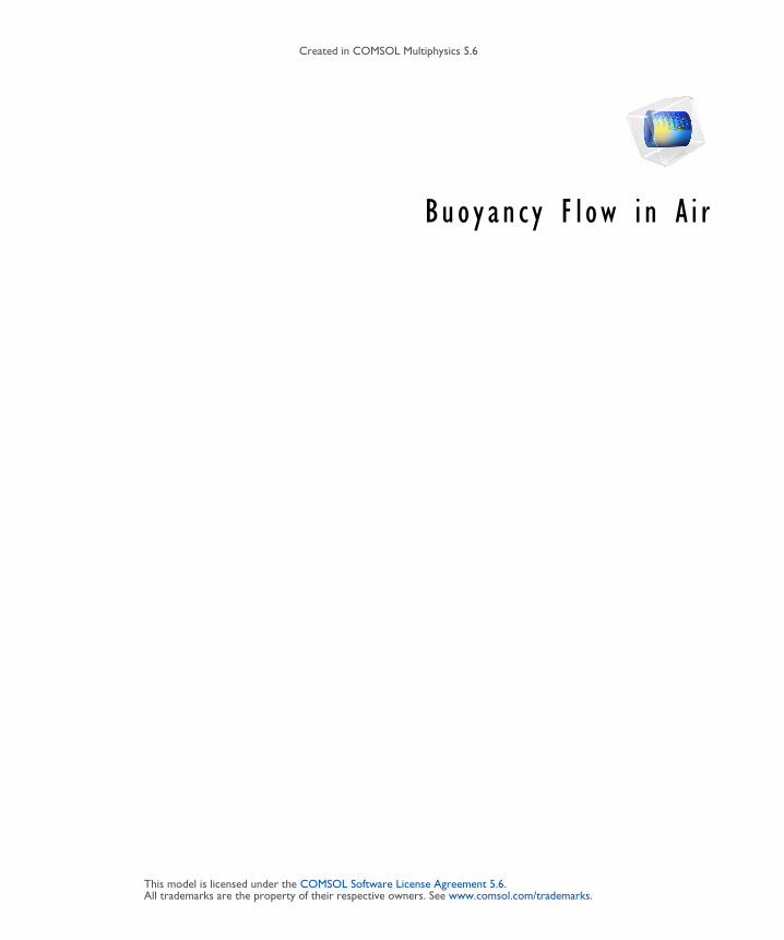
The 3D model (see Figure 2) extends the geometry to a cube. Compared to the 2D model, the front and back sides are additional boundaries that may influence the fluid behavior.

Figure 2: Domain geometry and boundary conditions for the 3D model (cubic cavity).

Both models calculate and compare the velocity field and the temperature field. The predefined Nonisothermal Flow interface available in the Heat Transfer Module provides appropriate tools to fully couple the heat transfer and the fluid dynamics.

Model Definition

2 D M O D E L

Figure 1 illustrates the 2D model geometry. The fluid fills a square cavity with impermeable walls, so the fluid flows freely within the cavity but cannot leak out. The right and left edges of the cavity are maintained at high and low temperatures, respectively. The upper and lower boundaries are insulated. The temperature differential produces the density variation that drives the buoyant flow.

The compressible Navier-Stokes equation contains a buoyancy term on the right-hand side to account for the lifting force due to thermal expansion that causes the density variations:

Air

Hot temperature (20 °C) on the right plate

Cold temperature (10 °C) on the left plate

Pressure point constraint (0 Pa)

Cube side length (10 cm)

ρ u ∇⋅( )u ∇p– ∇ μ ∇u ∇u( )T+( ) 2

3---μ ∇ u⋅( )– ρg+⋅+=


In this expression, the dependent variables for flow are the fluid velocity vector, u, and the pressure, p. The constant g denotes the gravitational acceleration, ρ gives the temperature-dependent density, and μ is the temperature-dependent dynamic viscosity.

Because the model only contains information about the pressure gradient, it estimates the pressure field up to a constant. To define this constant, you arbitrarily fix the pressure at a point. No slip boundary conditions apply on all boundaries. The no slip condition results in zero velocity at the wall but does not set any constraint on p.

At steady-state, the heat balance for a fluid reduces to the following equation:

Here T represents the temperature, k denotes the thermal conductivity, and Cp is the specific heat capacity of the fluid.

The boundary conditions for the heat transfer interface are the fixed high and low temperatures on the vertical walls with insulation conditions elsewhere, as shown in Figure 1.

3 D M O D E L

Figure 2 shows the geometry and boundary conditions of the 3D model. The cavity is now a cube with high and low temperatures applied respectively at the right and left surfaces. The remaining boundaries (top, bottom, front, and back) are thermally insulated.

I N D I C A T O R S O F T H E F L O W R E G I M E

Before starting the simulations, it is recommended to estimate the flow regime. The Grashof number, Rayleigh number, and Prandtl number are then computed and summarized in Table 1 below.

See the model analysis in Buoyancy Flow in Water for more details about the definition of these indicators.

The Grashof and Rayleigh numbers are about 106, and thus significantly below the critical value of 109 for the flow to become turbulent between vertical plates (see Ref. 1). A laminar regime is therefore expected.

TABLE 1: INDICATORS OF THE FLOW REGIME.

Indicator Description Value

Gr Grashof number 1.6·106

Ra Rayleigh number 1.1·106

Pr Prandtl number 0.7

ρCpu ∇T⋅ ∇– k T∇( )⋅ 0=


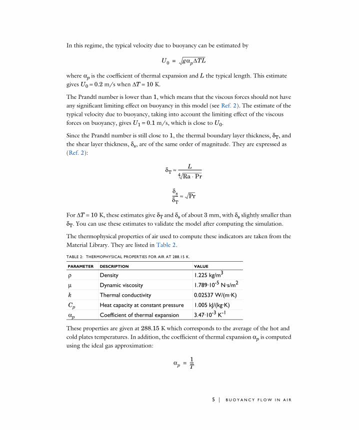
In this regime, the typical velocity due to buoyancy can be estimated by

where αp is the coefficient of thermal expansion and L the typical length. This estimate gives U0 = 0.2 m/s when ΔT = 10 K.

The Prandtl number is lower than 1, which means that the viscous forces should not have any significant limiting effect on buoyancy in this model (see Ref. 2). The estimate of the typical velocity due to buoyancy, taking into account the limiting effect of the viscous forces on buoyancy, gives U1 = 0.1 m/s, which is close to U0.

Since the Prandtl number is still close to 1, the thermal boundary layer thickness, δT, and the shear layer thickness, δs, are of the same order of magnitude. They are expressed as (Ref. 2):

For ΔT = 10 K, these estimates give δT and δs of about 3 mm, with δs slightly smaller than δT. You can use these estimates to validate the model after computing the simulation.

The thermophysical properties of air used to compute these indicators are taken from the Material Library. They are listed in Table 2.

These properties are given at 288.15 K which corresponds to the average of the hot and cold plates temperatures. In addition, the coefficient of thermal expansion αp is computed using the ideal gas approximation:

TABLE 2: THERMOPHYSICAL PROPERTIES FOR AIR AT 288.15 K.

PARAMETER DESCRIPTION VALUE

ρ Density 1.225 kg/m3

μ Dynamic viscosity 1.789·10-5 N·s/m2

k Thermal conductivity 0.02537 W/(m·K)

Cp Heat capacity at constant pressure 1.005 kJ/(kg·K)

αp Coefficient of thermal expansion 3.47·10-3 K-1

U0 gαpΔTL=

δTL

Ra Pr⋅4------------------------≈

δsδT------ Pr≈

αp1T----=


By using the average of the hot and cold plate temperatures in this approximation, you get αp = 3.47·10−3 K−1.

Results and Discussion

2 D M O D E L

Figure 3 shows the velocity distribution in the square cavity.

Figure 3: Velocity magnitude for the 2D model.

The regions with faster velocities are located at the lateral boundaries. The maximum velocity is 0.05 m/s which is a bit lower than the estimated typical velocity U0 = 0.2 m/s, but still in the same order of magnitude. According to Figure 4, the shear layer thickness is about 3 mm, as calculated previously.


Figure 4: Velocity profile at the left boundary.


Figure 5 shows the temperature field (surface) and velocity field (arrows) of the 2D model.

Figure 5: Temperature field (surface plot) and velocity (arrows) for the 2D model.

A large convective cell occupies the whole square. The fluid flow follows the boundaries. As seen in Figure 3, it is faster at the vertical plates where the highest variations of


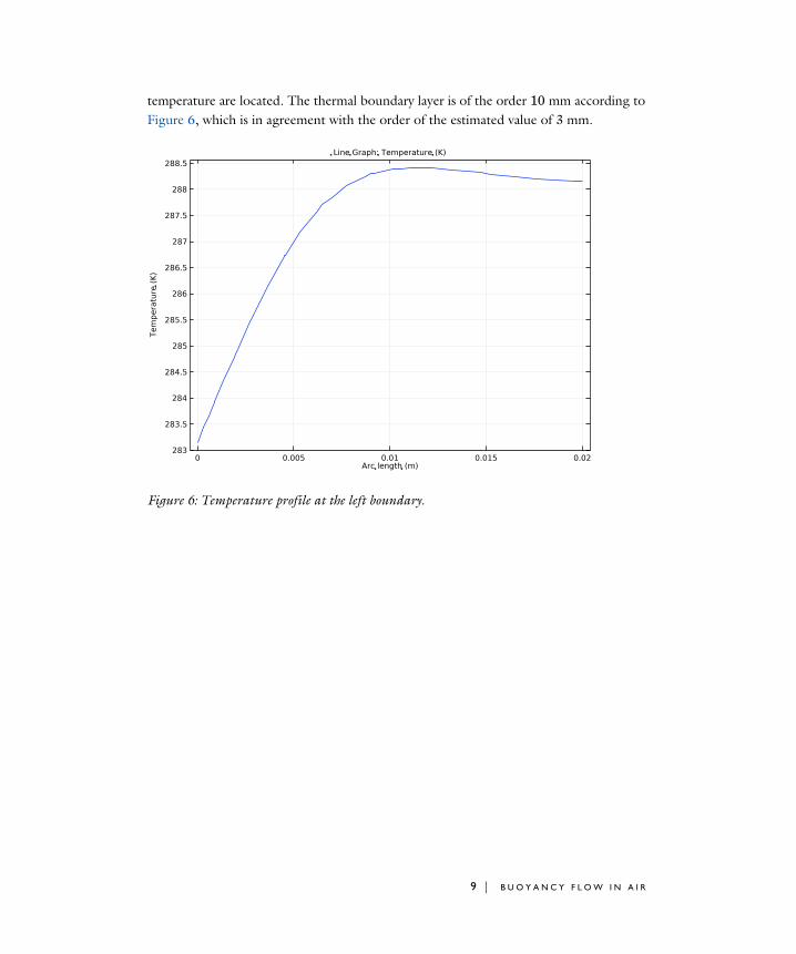
temperature are located. The thermal boundary layer is of the order 10 mm according to Figure 6, which is in agreement with the order of the estimated value of 3 mm.

Figure 6: Temperature profile at the left boundary.


3 D M O D E L

Figure 7 illustrates the velocity plot parallel to the heated plates.

Figure 7: Velocity magnitude field for the 3D model, slices parallel to the heated plates.


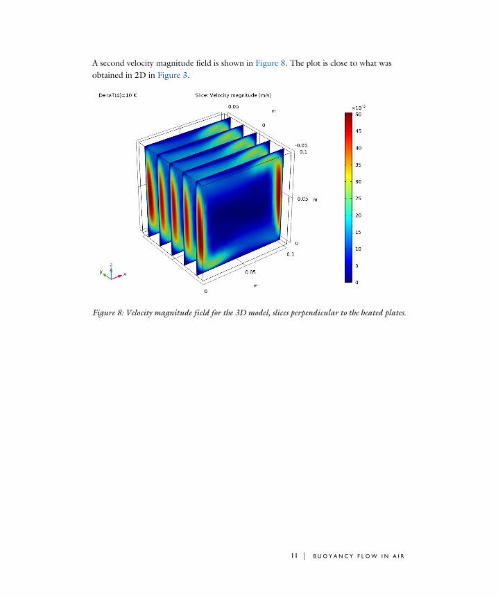
A second velocity magnitude field is shown in Figure 8. The plot is close to what was obtained in 2D in Figure 3.

Figure 8: Velocity magnitude field for the 3D model, slices perpendicular to the heated plates.


In Figure 9, velocity arrows are plotted on temperature surface at the middle vertical plane parallel to the plates.

Figure 9: Temperature (surface plot) and velocity (arrows) fields in the cubic cavity, for a temperature difference of 10 K between the vertical plates.

New small convective cells appear on the vertical planes perpendicular to the plates at the four corners.

Notes About the COMSOL Implementation

The material properties for air are available in the Material Library.

At high Gr values, using a good initial condition becomes important in order to achieve convergence. Moreover, a well-tuned mesh is needed to capture the solution, especially the temperature and velocity changes near the walls. Use the Stationary study step’s continuation option with ΔT as the continuation parameter to get a solver sequence that uses previous solutions to estimate the initial condition. For this tutorial, it is appropriate to ramp up ΔT from 10−2 K to 10 K, which corresponds to a Grashof number range of 103–106. At Gr = 103, the model is easy to solve. The regime is dominated by conduction. At Gr = 106, the model becomes more difficult to solve. The regime is more influenced by convection and buoyancy.


To get a well-tuned mesh when Gr reaches 106, the element size near the prescribed temperature boundaries has to be smaller than the shear layer and thermal boundary layer thicknesses, which are of order 3 mm. It is recommended to have three to five elements across the layers when using P1 elements (the default setting for fluid flows).

References

1. F.P. Incropera, D.P. DeWitt, T.L. Bergman, and A.S. Lavine, Fundamentals of Heat and Mass Transfer, 6th ed., John Wiley & Sons, 2006.

2. A. Bejan, Heat Transfer, John Wiley & Sons, 1993.

Application Library path: Heat_Transfer_Module/Tutorials,_Forced_and_Natural_Convection/buoyancy_air

Modeling Instructions

From the File menu, choose New.

N E W

In the New window, click Model Wizard.

M O D E L W I Z A R D

1 In the Model Wizard window, click 2D.

2 In the Select Physics tree, select Fluid Flow>Nonisothermal Flow>Laminar Flow.

3 Click Add.

4 Click Study.

5 In the Select Study tree, select General Studies>Stationary.

6 Click Done.

G L O B A L D E F I N I T I O N S

Parameters 11 In the Model Builder window, under Global Definitions click Parameters 1.

2 In the Settings window for Parameters, locate the Parameters section.


3 In the table, enter the following settings:

Name Expression Value Description

L 10[cm] 0.1 m Square side length

W L/2 0.05 m Volume thickness

DeltaT 10[K] 10 K Temperature difference

Tc 283.15[K] 283.15 K Low temperature

Th Tc+DeltaT 293.15 K High temperature

T_avg (Tc+Th)/2 288.15 K Average temperature approximation

p_ref 1[atm] 1.0133E5 Pa Reference pressure

p0 0[Pa] 0 Pa Relative pressure constraint

dt_range_start

-2 -2 Range start point of the parametric sweep on DeltaT (log10 of the value in K)

dt_range_stop 1 1 Range end point of the parametric sweep on DeltaT (log10 of the value in K)

rho 1.225[kg/m^3] 1.225 kg/m³ Density at T_avg and 1 atm

mu 1.789e-5[N*s/m^2]

1.789E-5 N·s/(m·m)

Dynamic viscosity at T_avg

k 0.02537[W/(m*K)] 0.02537 W/(m·K) Thermal conductivity at T_avg

Cp 1.005[kJ/(kg*K)] 1005 J/(kg·K) Heat capacity at T_avg

alpha 1/T_avg 0.0034704 1/K Coefficient of thermal expansion at T_avg

U0 sqrt(g_const*alpha*DeltaT*L)

0.18448 m/s Typical velocity due to buoyancy

U1 U0/sqrt(Pr) 0.21914 m/s Typical velocity due to buoyancy

Pr mu*Cp/k 0.70869 Prandtl number


The Grashof and Rayleigh numbers are less than 109, indicating that a laminar regime is expected.

G E O M E T R Y 1

Square 1 (sq1)1 In the Geometry toolbar, click Square.

2 In the Settings window for Square, locate the Size section.

3 In the Side length text field, type L.

4 In the Geometry toolbar, click Build All.

A D D M A T E R I A L

1 In the Home toolbar, click Add Material to open the Add Material window.

2 Go to the Add Material window.

3 In the tree, select Built-in>Air.

4 Click Add to Component in the window toolbar.

5 In the Home toolbar, click Add Material to close the Add Material window.

L A M I N A R F L O W ( S P F )

In order to ensure mass conservation, as the volume is constant, the air density cannot depend only on the temperature. It has to be either constant or pressure and temperature dependent. In this model the density variations are small and you can make the incompressible assumption.

1 In the Model Builder window, under Component 1 (comp1) click Laminar Flow (spf).

2 In the Settings window for Laminar Flow, locate the Physical Model section.

3 From the Compressibility list, choose Incompressible flow.

Gr (U0*rho*L/mu)^2 1.5957E6 Grashof number

Ra Pr*Gr 1.1309E6 Rayleigh number

eps_t L/(Pr*Ra)^0.25 0.0033422 m Thermal boundary layer thickness

eps_s eps_t*sqrt(Pr) 0.0028136 m Shear layer thickness

Name Expression Value Description


4 Select the Include gravity check box.

The absolute pressure distribution is pA = pref + p, p being the variable solved for.

The pressure p is automatically initialized at p0 +ρ gz.

5 In the pref text field, type p_ref.

Set the reference point for gravity at the top of the square, so that the ρgz term of the pressure is 0 at this point.

6 Specify the rref vector as

Initial Values 11 In the Model Builder window, under Component 1 (comp1)>Laminar Flow (spf) click

Initial Values 1.

2 In the Settings window for Initial Values, locate the Initial Values section.

3 In the p text field, type p0.

Fixing the pressure at an arbitrary point is necessary to define a well-posed model. Use a Pressure Point Constraint that locks the pressure at the upper-left corner.

Pressure Point Constraint 11 In the Physics toolbar, click Points and choose Pressure Point Constraint.

2 Select Point 2 only.

3 In the Settings window for Pressure Point Constraint, locate the Pressure Constraint section.

4 In the p0 text field, type p0.

H E A T T R A N S F E R I N F L U I D S ( H T )

Set the reference temperature to the mean temperature between heated faces.

This value along with the reference pressure determines the reference density used to initialize the pressure pinit.

1 In the Model Builder window, under Component 1 (comp1) click Heat Transfer in Fluids (ht).

2 In the Settings window for Heat Transfer in Fluids, locate the Physical Model section.

3 In the Tref text field, type T_avg.

0 x

L y


Initial Values 1Define the initial temperature as the mean value between the high and low temperature values.

1 In the Model Builder window, under Component 1 (comp1)>Heat Transfer in Fluids (ht) click Initial Values 1.


3 In the T text field, type T_avg.

Now define the temperature constraints on the vertical walls.

Temperature 11 In the Physics toolbar, click Boundaries and choose Temperature.

2 Select Boundary 1 only.

3 In the Settings window for Temperature, locate the Temperature section.

4 In the T0 text field, type Tc.




4 In the T0 text field, type Th.

M U L T I P H Y S I C S

Nonisothermal Flow 1 (nitf1)1 In the Model Builder window, under Component 1 (comp1)>Multiphysics click

Nonisothermal Flow 1 (nitf1).

2 In the Settings window for Nonisothermal Flow, locate the Material Properties section.

3 Select the Boussinesq approximation check box.

M E S H 1

Now, modify the default mesh size settings to ensure that the mesh satisfies the criterion discussed in the Introduction section.

1 In the Model Builder window, under Component 1 (comp1) click Mesh 1.

2 In the Settings window for Mesh, locate the Physics-Controlled Mesh section.

3 From the Element size list, choose Extra fine.

4 Click Build All.


S T U D Y 1

Step 1: Stationary1 In the Model Builder window, under Study 1 click Step 1: Stationary.

2 In the Settings window for Stationary, click to expand the Study Extensions section.

3 Select the Auxiliary sweep check box.

4 Click Add.


6 Click Range.

7 In the Range dialog box, type dt_range_start in the Start text field.

8 In the Step text field, type 1.

9 In the Stop text field, type dt_range_stop.

10 From the Function to apply to all values list, choose exp10(x) –Exponential function (base 10).

11 Click Replace.

12 In the Settings window for Stationary, locate the Study Extensions section.


14 In the Model Builder window, click Study 1.

15 In the Settings window for Study, type Study 2D in the Label text field.

16 Click the Show More Options button in the Model Builder toolbar.

17 In the Show More Options dialog box, in the tree, select the check box for the node Physics>Advanced Physics Options.

18 Click OK.

L A M I N A R F L O W ( S P F )

The pseudo time stepping option is generally useful to help the convergence of a stationary flow model. However, a continuation approach is already used here. In this particular

Parameter name Parameter value list Parameter unit

DeltaT (Temperature difference) K


DeltaT (Temperature difference) 10^{range(dt_range_start,1,dt_range_stop)}

K


model, disabling the pseudo time stepping option improves the convergence. Follow the instructions below to do so.

1 In the Model Builder window, under Component 1 (comp1) click Laminar Flow (spf).

2 In the Settings window for Laminar Flow, click to expand the Advanced Settings section.

3 Find the Pseudo time stepping subsection. From the Use pseudo time stepping for stationary equation form list, choose Off.

4 In the Home toolbar, click Compute.

R E S U L T S

Velocity (spf)The first default plot group shows the velocity magnitude as in Figure 3. Notice the high velocities near the lateral walls due to buoyancy effects.

Temperature (ht)The third default plot shows the temperature distribution. Add arrows of the velocity field to see the correlations between velocity and temperature, as in Figure 5.

Arrow Surface 11 In the Model Builder window, right-click Temperature (ht) and choose Arrow Surface.

2 In the Settings window for Arrow Surface, locate the Coloring and Style section.

3 From the Color list, choose Black.

4 In the Temperature (ht) toolbar, click Plot.

In the following steps, the temperature and velocity profiles are plotted near the left boundary in order to estimate the boundary layer thicknesses of the solution.

Cut Line 2D 11 In the Results toolbar, click Cut Line 2D.

2 In the Settings window for Cut Line 2D, locate the Line Data section.

3 In row Point 2, set x to L/5.

4 In row Point 1, set y to L/2.

5 In row Point 2, set y to L/2.

Temperature at Boundary Layer1 In the Results toolbar, click 1D Plot Group.

2 In the Settings window for 1D Plot Group, type Temperature at Boundary Layer in the Label text field.


3 Locate the Data section. From the Dataset list, choose Cut Line 2D 1.

4 From the Parameter selection (DeltaT) list, choose From list.

5 In the Parameter values (DeltaT (K)) list, select 10.

Line Graph 11 Right-click Temperature at Boundary Layer and choose Line Graph.

2 In the Settings window for Line Graph, click Replace Expression in the upper-right corner of the y-Axis Data section. From the menu, choose Component 1 (comp1)>

Heat Transfer in Fluids>Temperature>T - Temperature - K.

3 In the Temperature at Boundary Layer toolbar, click Plot.

The thermal boundary layer thickness is around 10 mm, which is in agreement with the order of the estimated value.

Velocity at Boundary Layer1 In the Home toolbar, click Add Plot Group and choose 1D Plot Group.

2 In the Settings window for 1D Plot Group, type Velocity at Boundary Layer in the Label text field.

3 Locate the Data section. From the Dataset list, choose Cut Line 2D 1.

4 From the Parameter selection (DeltaT) list, choose From list.

5 In the Parameter values (DeltaT (K)) list, select 10.

Line Graph 11 Right-click Velocity at Boundary Layer and choose Line Graph.

2 In the Velocity at Boundary Layer toolbar, click Plot.

The shear layer thickness is around 3 mm, which is in good agreement with the estimated value.

R O O T

Now create the 3D version of the model.

A D D C O M P O N E N T

In the Model Builder window, right-click the root node and choose Add Component>3D.

A D D P H Y S I C S

1 In the Home toolbar, click Add Physics to open the Add Physics window.

2 Go to the Add Physics window.

3 In the tree, select Fluid Flow>Nonisothermal Flow>Laminar Flow.


4 Find the Physics interfaces in study subsection. In the table, clear the Solve check box for Study 2D.

5 Click Add to Component 2 in the window toolbar.

6 In the Home toolbar, click Add Physics to close the Add Physics window.

A D D S T U D Y

1 In the Home toolbar, click Add Study to open the Add Study window.

2 Go to the Add Study window.

3 Find the Studies subsection. In the Select Study tree, select General Studies>Stationary.

4 Find the Physics interfaces in study subsection. In the table, clear the Solve check boxes for Laminar Flow (spf) and Heat Transfer in Fluids (ht).

5 Find the Multiphysics couplings in study subsection. In the table, clear the Solve check box for Nonisothermal Flow 1 (nitf1).

6 Click Add Study in the window toolbar.

7 In the Home toolbar, click Add Study to close the Add Study window.

G E O M E T R Y 2

Block 1 (blk1)1 In the Geometry toolbar, click Block.

2 In the Settings window for Block, locate the Size and Shape section.

3 In the Width text field, type L.

4 In the Depth text field, type L/2.

5 In the Height text field, type L.

6 In the Geometry toolbar, click Build All.

A D D M A T E R I A L

1 In the Home toolbar, click Add Material to open the Add Material window.

2 Go to the Add Material window.

3 In the tree, select Built-in>Air.

4 Click Add to Component in the window toolbar.

5 In the Home toolbar, click Add Material to close the Add Material window.

L A M I N A R F L O W 2 ( S P F 2 )

1 In the Model Builder window, under Component 2 (comp2) click Laminar Flow 2 (spf2).


2 In the Settings window for Laminar Flow, locate the Physical Model section.

3 From the Compressibility list, choose Incompressible flow.

4 Select the Include gravity check box.

5 In the pref text field, type p_ref.

6 Specify the rref vector as

Initial Values 11 In the Model Builder window, under Component 2 (comp2)>Laminar Flow 2 (spf2) click

Initial Values 1.


3 In the p text field, type p0.

Pressure Point Constraint 11 In the Physics toolbar, click Points and choose Pressure Point Constraint.

2 Select Point 4 only.

Symmetry 11 In the Physics toolbar, click Boundaries and choose Symmetry.


The solution will be evaluated for the geometry (here, a cube) with a symmetry plane at the selected boundary.

H E A T T R A N S F E R I N F L U I D S 2 ( H T 2 )

1 In the Model Builder window, under Component 2 (comp2) click Heat Transfer in Fluids 2 (ht2).

2 In the Settings window for Heat Transfer in Fluids, locate the Physical Model section.

3 In the Tref text field, type T_avg.

Initial Values 11 In the Model Builder window, under Component 2 (comp2)>Heat Transfer in Fluids 2 (ht2)

click Initial Values 1.


3 In the T2 text field, type T_avg.

0 x

0 y

L z





4 In the T0 text field, type Tc.




4 In the T0 text field, type Th.

Symmetry 11 In the Physics toolbar, click Boundaries and choose Symmetry.


M U L T I P H Y S I C S

Nonisothermal Flow 2 (nitf2)1 In the Model Builder window, under Component 2 (comp2)>Multiphysics click

Nonisothermal Flow 2 (nitf2).

2 In the Settings window for Nonisothermal Flow, locate the Material Properties section.

3 Select the Boussinesq approximation check box.

M E S H 2

To obtain reliable results within a short computing time, create a structured mesh by following the steps below.

Mapped 11 In the Mesh toolbar, click Boundary and choose Mapped.


Distribution 11 Right-click Mapped 1 and choose Distribution.

2 Select Edges 1, 3, 5, and 9 only.

3 In the Settings window for Distribution, locate the Distribution section.

4 From the Distribution type list, choose Predefined.

5 In the Number of elements text field, type 16.


6 In the Element ratio text field, type 3.

7 Select the Symmetric distribution check box.

Swept 1In the Mesh toolbar, click Swept.

Distribution 11 Right-click Swept 1 and choose Distribution.

2 In the Settings window for Distribution, locate the Distribution section.

3 From the Distribution type list, choose Predefined.

4 In the Number of elements text field, type 8.

5 In the Element ratio text field, type 3.

6 Select the Reverse direction check box.

To resolve the boundary layers, use a Boundary Layers feature to generate smaller mesh elements near the walls.

The thermal boundary layer for the temperature difference of 10 K is approximately 3 mm (see the variable eps_t defined previously).

Use this value to define the thickness of the boundary layers, and divide the boundary layer in 5 mesh layers of increasing size.

Boundary Layers 1In the Mesh toolbar, click Boundary Layers.

Boundary Layer Properties1 In the Model Builder window, click Boundary Layer Properties.

2 Select Boundaries 1 and 3–6 only.

3 In the Settings window for Boundary Layer Properties, locate the Boundary Layer Properties section.

4 In the Number of boundary layers text field, type 5.

5 From the Thickness of first layer list, choose Manual.

6 In the Thickness text field, type 3[mm]/5.

7 Click Build All.

S T U D Y 2

Step 1: Stationary1 In the Model Builder window, under Study 2 click Step 1: Stationary.



3 Select the Auxiliary sweep check box.

4 Click Add.


6 Click Range.

7 In the Range dialog box, type dt_range_start in the Start text field.

8 In the Step text field, type 1.

9 In the Stop text field, type dt_range_stop.

10 From the Function to apply to all values list, choose exp10(x) –Exponential function (base 10).

11 Click Replace.



The continuation solver works best for models with linear dependence on the parameter. A more robust alternative for nonlinear applications is to start from the solution for the previous parameter value.

1 From the Run continuation for list, choose No parameter.

2 From the Reuse solution from previous step list, choose Yes.

3 In the Model Builder window, click Study 2.

4 In the Settings window for Study, type Study 3D in the Label text field.

5 In the Home toolbar, click Compute.

R E S U L T S

Velocity (spf2)The default plot group shows the fluid velocity magnitude in only half of the cube. To plot the other half, proceed as follows.


DeltaT (Temperature difference) K


DeltaT (Temperature difference) 10^{range(dt_range_start,1,dt_range_stop)}

K


Mirror 3D 11 In the Results toolbar, click More Datasets and choose Mirror 3D.

2 In the Settings window for Mirror 3D, locate the Plane Data section.

3 From the Plane list, choose zx-planes.

A new dataset containing mirror values is now created. Go back to the velocity plot to use this dataset.

Slice1 In the Model Builder window, expand the Results>Velocity (spf2) node, then click Slice.

2 In the Settings window for Slice, click to expand the Quality section.

3 From the Resolution list, choose Fine.

Velocity (spf2)1 In the Model Builder window, click Velocity (spf2).

2 In the Settings window for 3D Plot Group, locate the Data section.

3 From the Dataset list, choose Mirror 3D 1.

4 In the Velocity (spf2) toolbar, click Plot.

5 Click Plot.

Pressure (spf2)1 In the Model Builder window, click Pressure (spf2).



4 In the Pressure (spf2) toolbar, click Plot.

Temperature (ht2)This default plot group shows the temperature distribution. The mirror dataset created previously can be reused here to plot the entire cube.

1 In the Model Builder window, click Temperature (ht2).



4 In the Temperature (ht2) toolbar, click Plot.

Isothermal Contours (ht2)1 In the Model Builder window, click Isothermal Contours (ht2).




4 In the Isothermal Contours (ht2) toolbar, click Plot.

Velocity, Front Plane1 In the Home toolbar, click Add Plot Group and choose 3D Plot Group.

2 In the Settings window for 3D Plot Group, type Velocity, Front Plane in the Label text field.

3 Locate the Data section. From the Dataset list, choose Mirror 3D 1.

Slice 11 Right-click Velocity, Front Plane and choose Slice.

2 In the Settings window for Slice, locate the Plane Data section.


4 In the Velocity, Front Plane toolbar, click Plot.

This slice view shows the velocity magnitude in the same plane as in the 2D model (Figure 8).

Next, plot arrows of the tangential velocity field in the vertical plane parallel to the plates to reproduce Figure 9.

Temperature, Velocity1 In the Home toolbar, click Add Plot Group and choose 3D Plot Group.

2 In the Settings window for 3D Plot Group, type Temperature, Velocity in the Label text field.

3 Locate the Data section. From the Dataset list, choose Mirror 3D 1.

Slice 11 Right-click Temperature, Velocity and choose Slice.

2 In the Settings window for Slice, locate the Expression section.

3 In the Expression text field, type T2.

4 Locate the Plane Data section. From the Entry method list, choose Coordinates.

5 In the x-coordinates text field, type L/2.

6 Locate the Coloring and Style section. From the Color table list, choose ThermalLight.

Arrow Volume 11 In the Model Builder window, right-click Temperature, Velocity and choose Arrow Volume.

2 In the Settings window for Arrow Volume, locate the Expression section.


3 In the x component text field, type 0.

4 Locate the Arrow Positioning section. Find the x grid points subsection. In the Points text field, type 1.

5 Find the y grid points subsection. In the Points text field, type 15.

6 Find the z grid points subsection. In the Points text field, type 15.

7 Locate the Coloring and Style section. From the Color list, choose Black.

8 In the Temperature, Velocity toolbar, click Plot.

Finally, you can switch to the main flow representation by adding the graphs as follows. Make sure to consider the arrow scale factor for any interpretation.

Slice 21 Right-click Temperature, Velocity and choose Slice.

2 In the Settings window for Slice, locate the Plane Data section.


4 From the Entry method list, choose Coordinates.

5 Locate the Expression section. In the Expression text field, type T2.

6 Locate the Coloring and Style section. From the Color table list, choose ThermalLight.

7 Click to expand the Inherit Style section. From the Plot list, choose Slice 1.


Arrow Volume 21 Right-click Temperature, Velocity and choose Arrow Volume.

2 In the Settings window for Arrow Volume, locate the Coloring and Style section.

3 From the Color list, choose Black.



Documents

Buoyancy Flow in Air