1

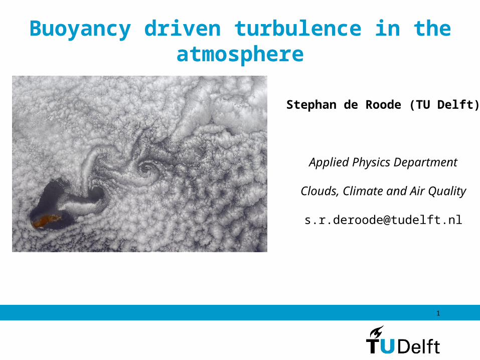
Buoyancy driven turbulence in the atmosphere

Stephan de Roode (TU Delft)

Applied Physics Department

Clouds, Climate and Air Quality

s.r.deroode@tudelft.nl

Multi-Scale Physics Faculty of Applied Sciences

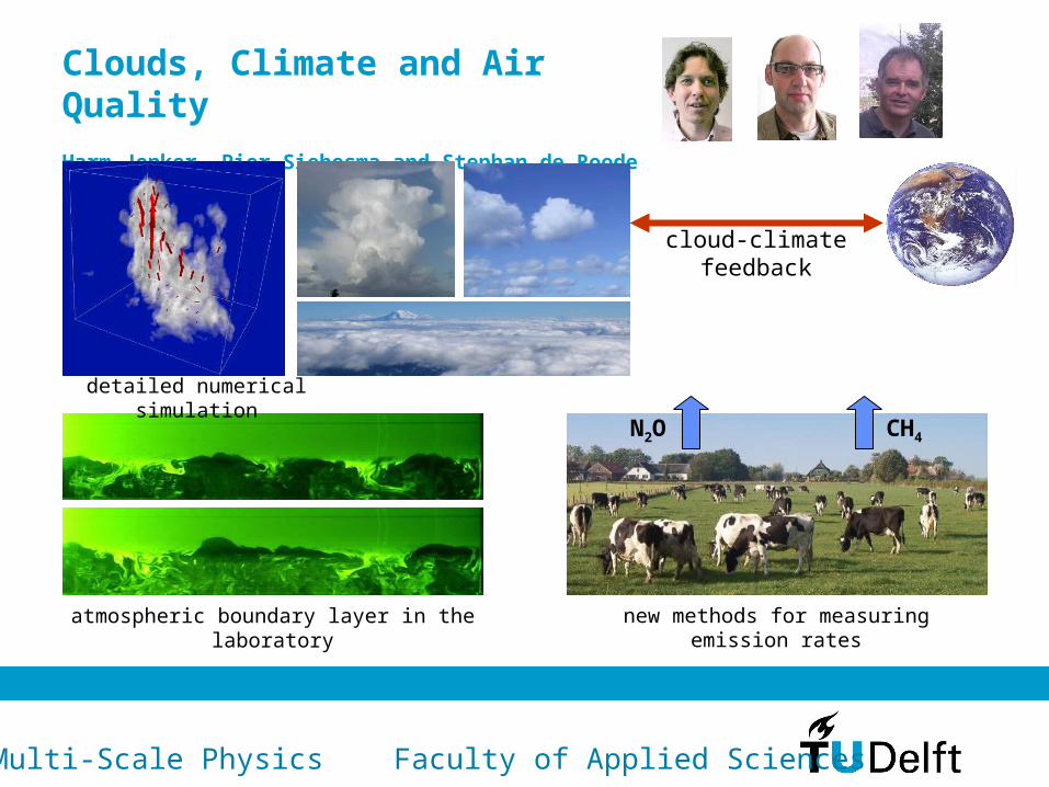
Clouds, Climate and Air Quality

Harm Jonker, Pier Siebesma and Stephan de Roode

atmospheric boundary layer in the laboratory

N2O CH4

new methods for measuring emission rates

cloud-climate feedback

detailed numerical simulation

3

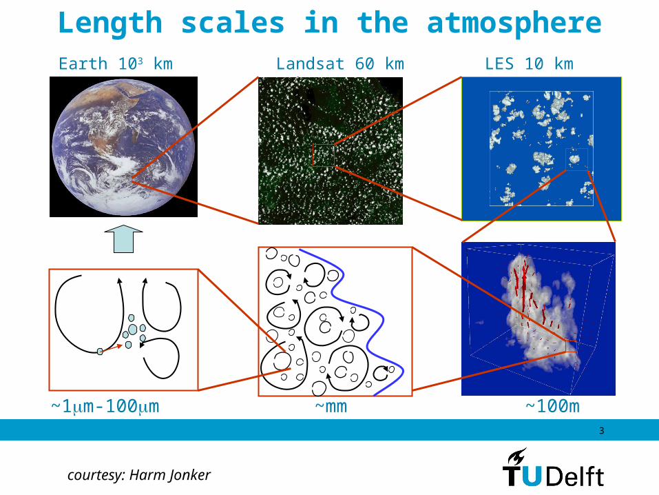
Length scales in the atmosphereLandsat 60 km 65km

LES 10 km

~mm ~100m~1m-100m

Earth 103 km

courtesy: Harm Jonker

4

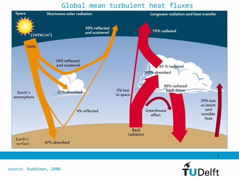
Global mean turbulent heat fluxes

source: Ruddiman, 2000

5

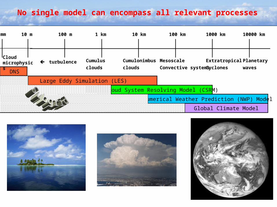
10 m 100 m 1 km 10 km 100 km 1000 km 10000 km

turbulence Cumulus

clouds

Cumulonimbus

clouds

Mesoscale

Convective systems

Extratropical

Cyclones

Planetary

waves

Large Eddy Simulation (LES) Model

Cloud System Resolving Model (CSRM)

Numerical Weather Prediction (NWP) Model

Global Climate Model

No single model can encompass all relevant processes

DNS

mm

Cloud microphysics

DALES: Dutch Atmospheric Large-Eddy Simulation Model

Dry LES code (prognostic subgrid TKE, stability dependent length scale)Frans Nieuwstadt (KNMI) and R. A. Brost (NOAA/NCAR, USA)

Radiation and moist thermodynamics Hans Cuijpers and Peter Duynkerke (KNMI/TU Delft, Utrecht University)

Parallellisation and Poisson solverMatthieu Pourquie and Bendiks Jan Boersma (TU Delft)

Drizzle Margreet Van Zanten and Pier Siebesma (UCLA/KNMI)

Atmospheric ChemistryJordi Vila (Wageningen University)

Land-surface interaction, advection schemesChiel van Heerwaarden (Wageningen University)

Particle dispersion, numericsThijs Heus and Harm Jonker (TU Delft)

7

Contents

Governing equations & static stability

Observations, large-eddy simulations and

parameterizations:

- Clear convection

- Latent heat release & shallow cumulus

- Longwave radiative cooling & stratocumulus

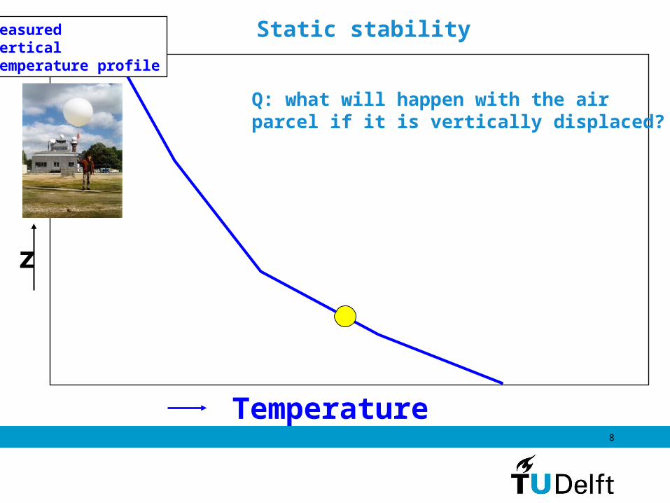
8

z

Temperature

Q: what will happen with the air parcel if it is vertically displaced?

Static stabilitymeasured vertical temperature profile

9

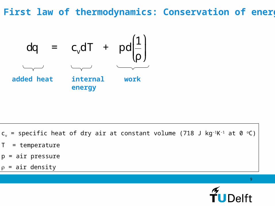
added heat internal energy

work

First law of thermodynamics: Conservation of energy

€

dq = cvdT + pd1ρ

⎛

⎝ ⎜

⎞

⎠ ⎟

cv = specific heat of dry air at constant volume (718 J kg-1K-1 at 0 oC)

T = temperature

p = air pressure

= air density

10

€

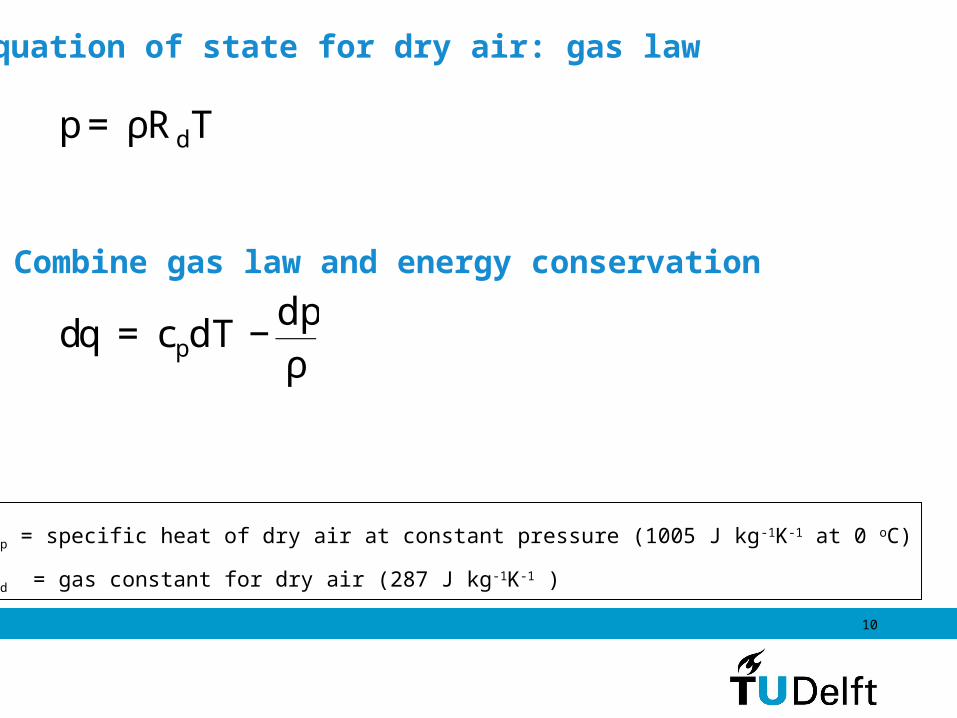
p = ρRdT

Equation of state for dry air: gas law

€

dq = cpdT −dpρ

Combine gas law and energy conservation

cp = specific heat of dry air at constant pressure (1005 J kg-1K-1 at 0 oC)

Rd = gas constant for dry air (287 J kg-1K-1 )

11

€

dpdz

= -ρg

Hydrostatic equilibrium

€

dq = cpdT +gdz

Gas law, energy conservation and hydrostatic equilibrium

Adiabatic process dq=0 dry adiabatic lapse rate

€

dTdz

= -gcp

= - Γd ≈ -9.8 K/km

12

z

F

F

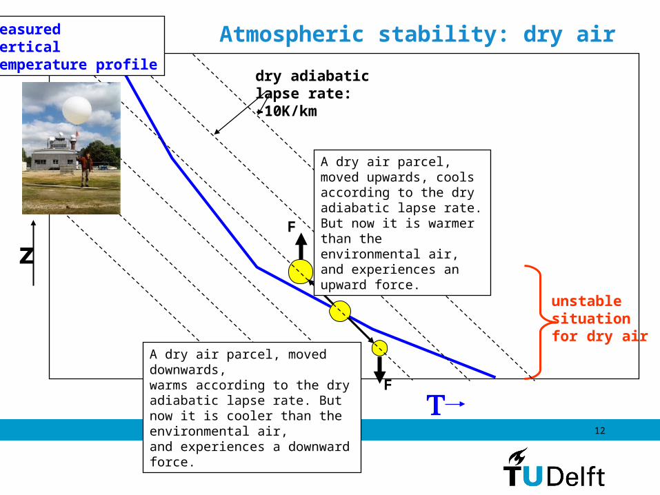
unstable situationfor dry air

dry adiabatic lapse rate: –10K/km

Atmospheric stability: dry air

A dry air parcel, moved upwards, cools according to the dry adiabatic lapse rate. But now it is warmer than the environmental air, and experiences an upward force.

A dry air parcel, moved downwards, warms according to the dry adiabatic lapse rate. But now it is cooler than the environmental air, and experiences a downward force.

measured vertical temperature profile

13

z

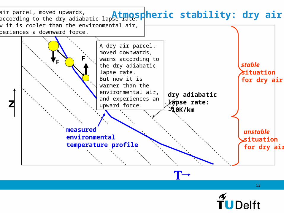
measured environmental temperature profile

unstable situationfor dry air

dry adiabatic lapse rate: –10K/km

FF

stable situationfor dry air

A dry air parcel, moved downwards, warms according to the dry adiabatic lapse rate. But now it is warmer than the environmental air, and experiences an upward force.

A dry air parcel, moved upwards, cools according to the dry adiabatic lapse rate. But now it is cooler than the environmental air, and experiences a downward force.

Atmospheric stability: dry air

14

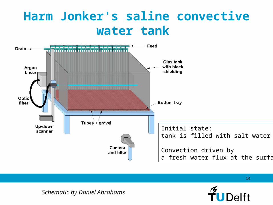
Harm Jonker's saline convective water tank

Schematic by Daniel Abrahams

Initial state:tank is filled with salt water

Convection driven bya fresh water flux at the surface

15

Convective water tank

Movie by Phillia Lijdsman

16

Adiabatic process dq=0 dry adiabatic lapse rate (2)

€

dq = cpdT −dpρ

= cpdT − RTdpp

= 0

€

θ(z) = T(z)p(z)p0

⎛

⎝ ⎜

⎞

⎠ ⎟

−Rd / cp

= cst

The potential temperature is the temperature if a parcel

would be brought adiabatically to a reference pressure p0

17

Balloon observations at Cabauw during daytime

Q: what makes this case challlenging for modeling?

18

LES results of a convective boundary layer: Buoyancy flux

€

∂w' w'∂t

= 2gθv

w' θv ' −∂w' w' w'

∂z−

2ρ

w'∂p'∂z

−2ν∂w'∂x j

⎛

⎝ ⎜

⎞

⎠ ⎟

2

€

gθv

w' θv ' = −gρ

w'ρ'

warm air going up

warm air going down

entrainment of warm air

Q: what is sign of the mean tendency for v?

19

LES results

Buoyancy flux and vertical velocity variance

€

∂w' w'∂t

= 2gθv

w' θv ' −∂w' w' w'

∂z−

2ρ

w'∂p'∂z

−2ν∂w'∂x j

⎛

⎝ ⎜

⎞

⎠ ⎟

2

20

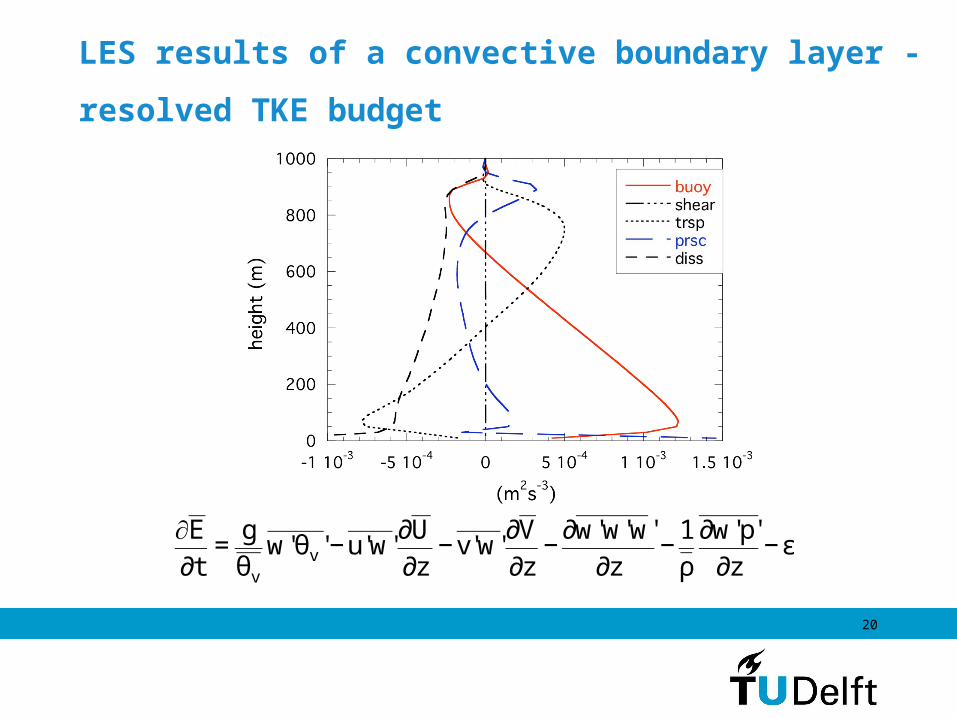
LES results of a convective boundary layer -

resolved TKE budget

€

∂E∂t

=gθv

w' θv ' −u' w'∂U∂z

−v' w'∂V∂z

−∂w' w' w'

∂z−

1ρ

∂w' p'∂z

−ε

21

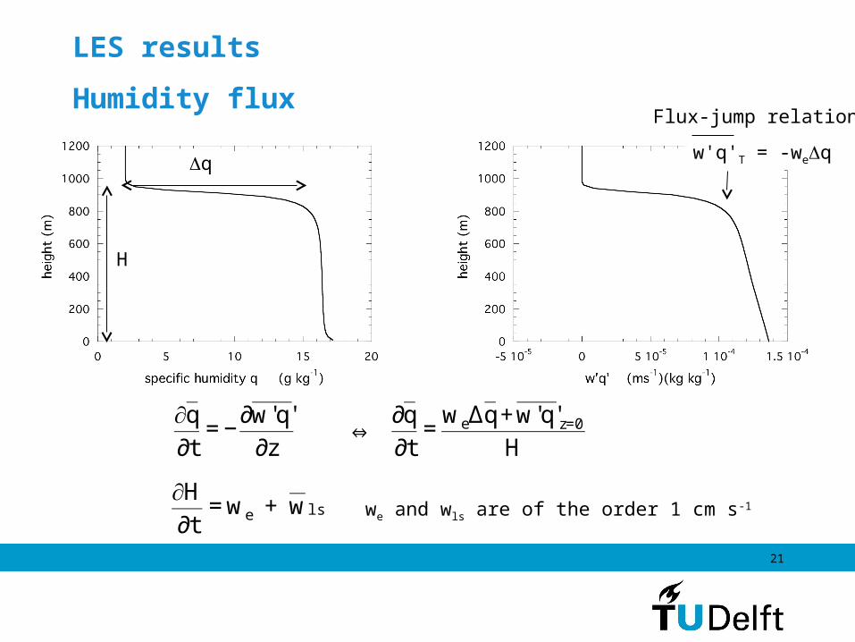
LES results

Humidity flux

qw'q'T = -weq

Flux-jump relation:

H

€

∂q∂t

= −∂w' q'

∂z ⇔

∂q∂t

=weΔq +w' q'z=0

H

€

∂H∂t

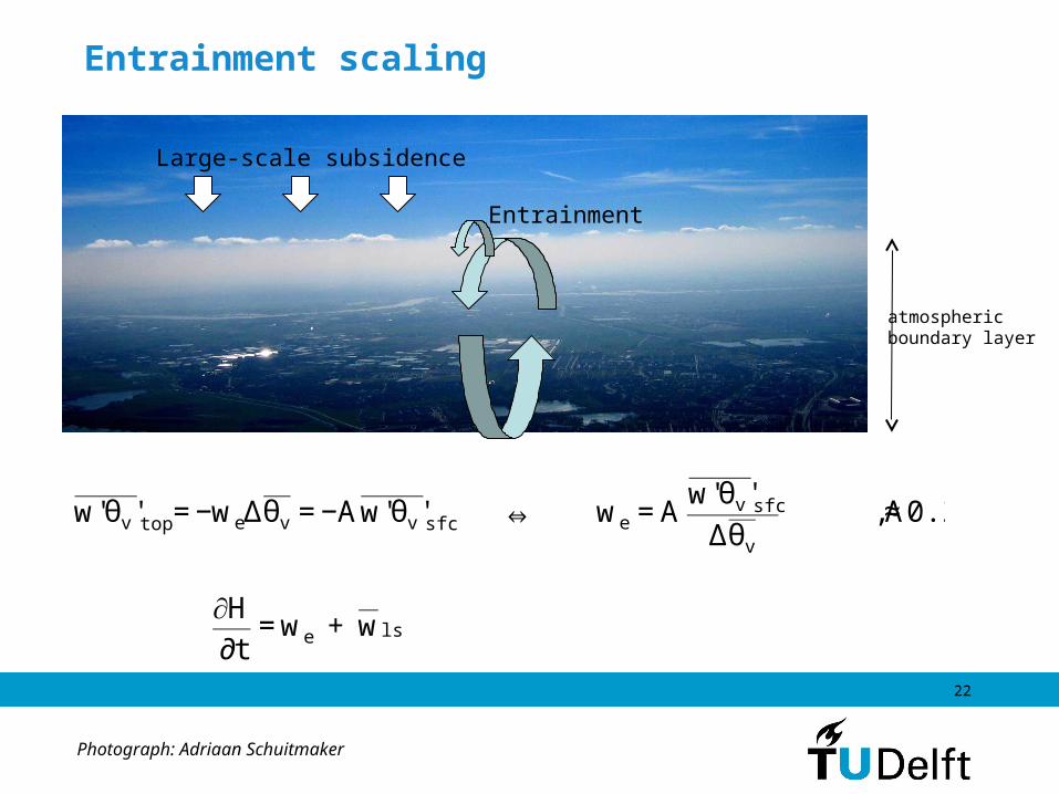
= we + w ls we and wls are of the order 1 cm s-1

22

Entrainment scaling

Photograph: Adriaan Schuitmaker

atmospheric boundary layer

Entrainment

Large-scale subsidence

€

w' θv ' top = −weΔθv = −Aw' θv 'sfc ⇔ we = Aw' θv 'sfc

Δθv

, A ≈ 0.2

€

∂H∂t

= we + w ls

23

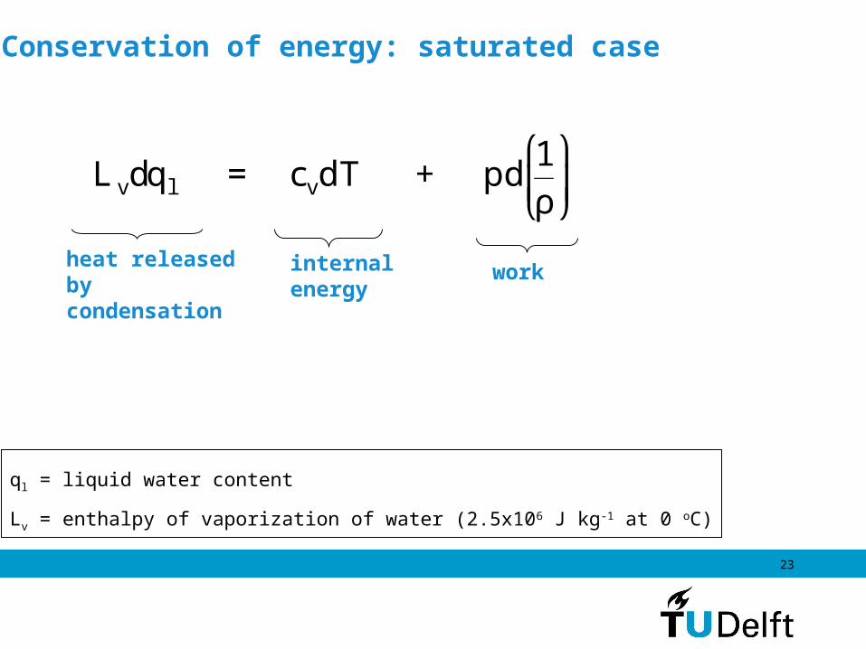
heat released by condensation

internal energy

work

Conservation of energy: saturated case

€

L vdq l = cvdT + pd1ρ

⎛

⎝ ⎜

⎞

⎠ ⎟

ql = liquid water content

Lv = enthalpy of vaporization of water (2.5x106 J kg-1 at 0 oC)

24

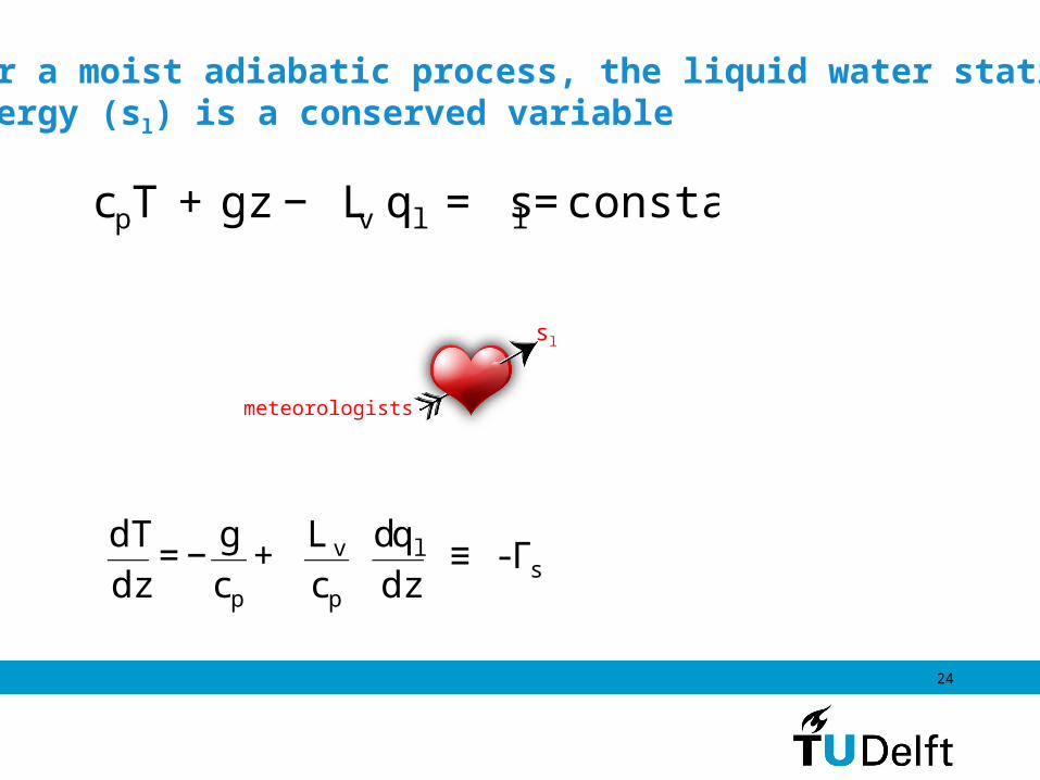
For a moist adiabatic process, the liquid water staticenergy (sl) is a conserved variable

€

cpT + gz − L v q l = sl = constant

meteorologists

sl

€

dTdz

= −gcp

+ L v

cp

dq l

dz ≡ - Γs

25

z

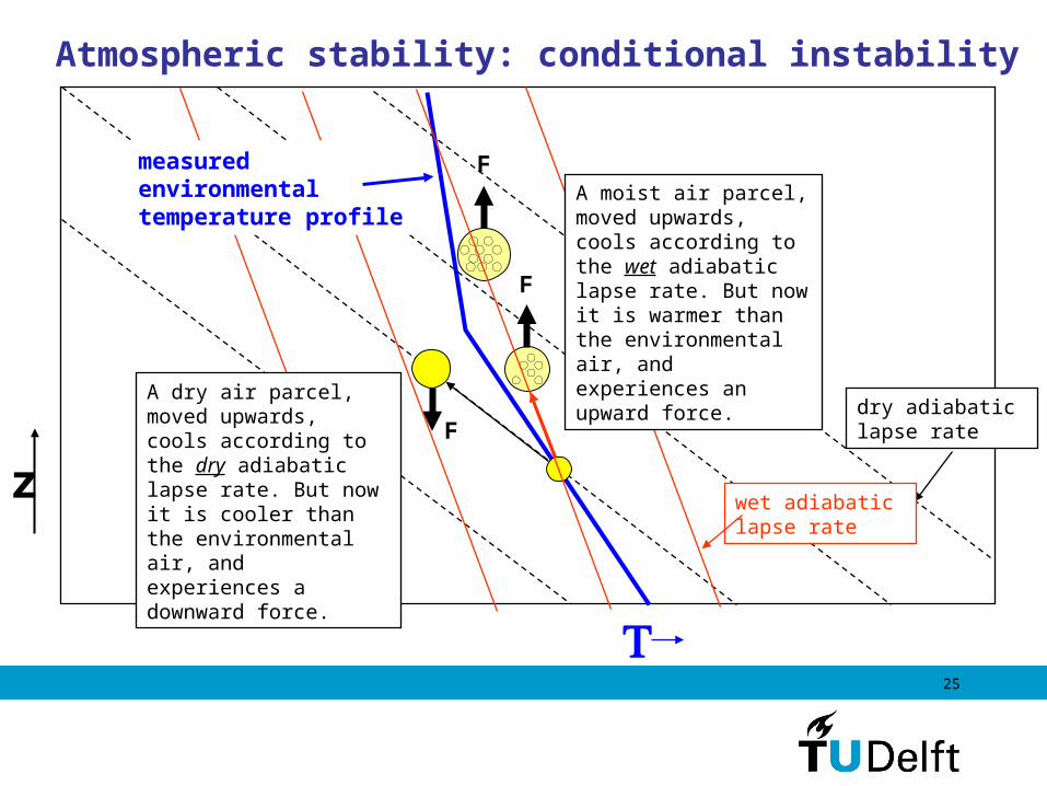
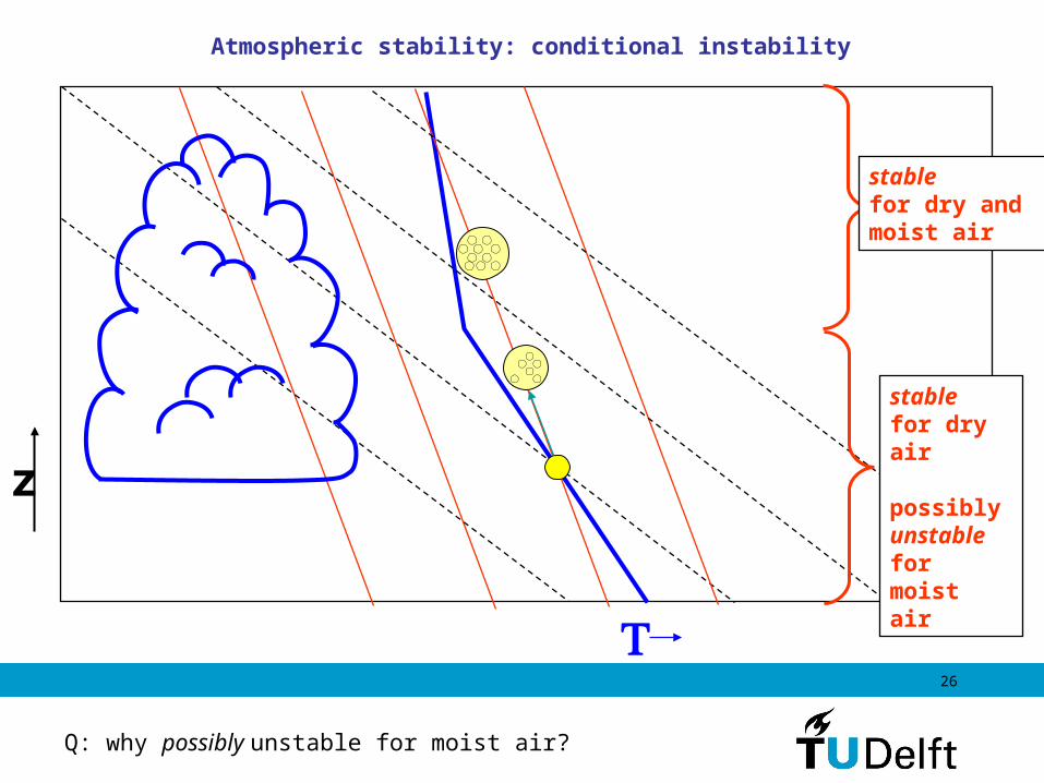
Atmospheric stability: conditional instability

F

F

F

dry adiabatic lapse rate

wet adiabatic lapse rate

measured environmental temperature profile

A moist air parcel, moved upwards, cools according to the wet adiabatic lapse rate. But now it is warmer than the environmental air, and experiences an upward force.

A dry air parcel, moved upwards, cools according to the dry adiabatic lapse rate. But now it is cooler than the environmental air, and experiences a downward force.

26

z

Atmospheric stability: conditional instability

stable for dry air

possiblyunstable for moist air

stable for dry and moist air

Q: why possibly unstable for moist air?

27

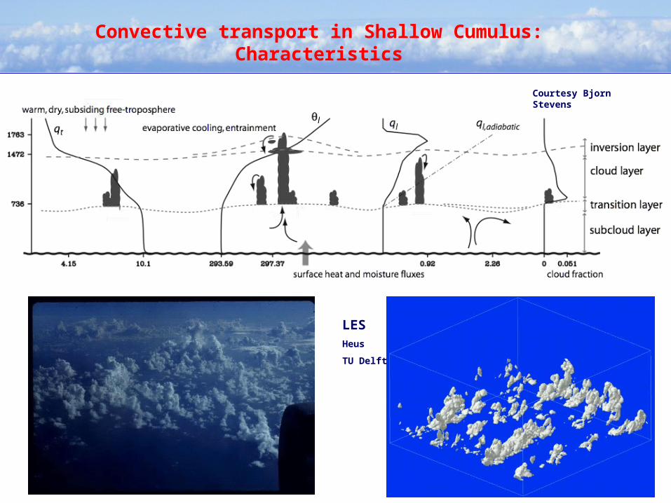
Convective transport in Shallow Cumulus: Characteristics

Courtesy Bjorn Stevens

LESHeus

TU Delft

28

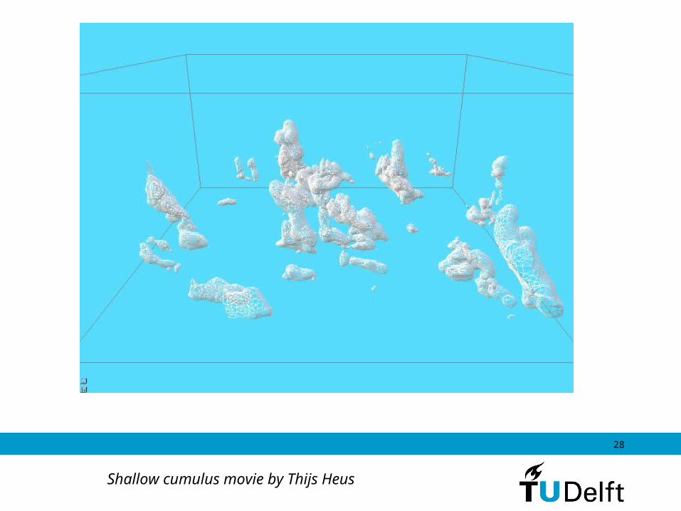
Shallow cumulus movie by Thijs Heus

29

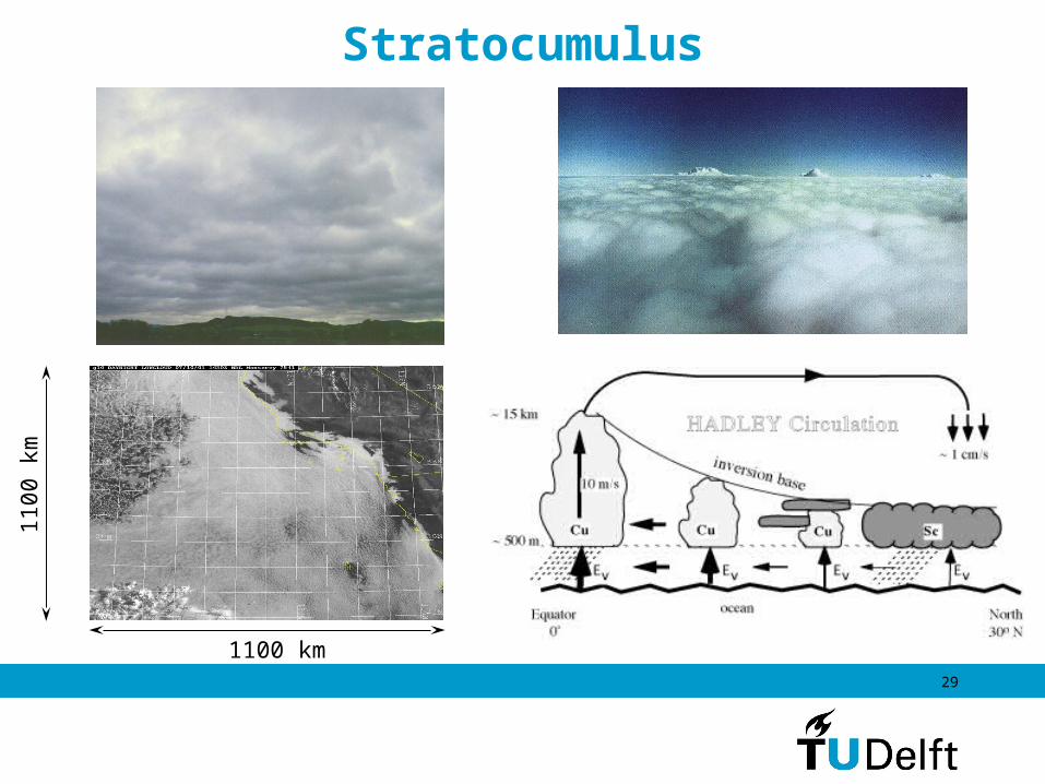
Stratocumulus1

10

0 k

m

1100 km

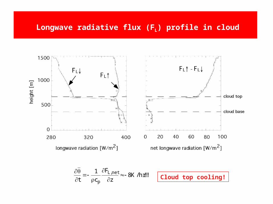
Longwave radiative flux (FL) profile in cloud

!!!hr/K8z

F

c

1

tnet,L

p

Cloud top cooling!

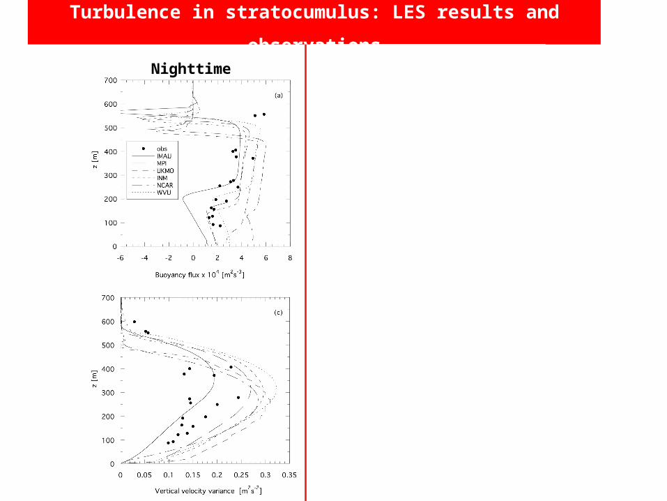
Turbulence in stratocumulus: LES results and

observationsNighttime Daytime

32

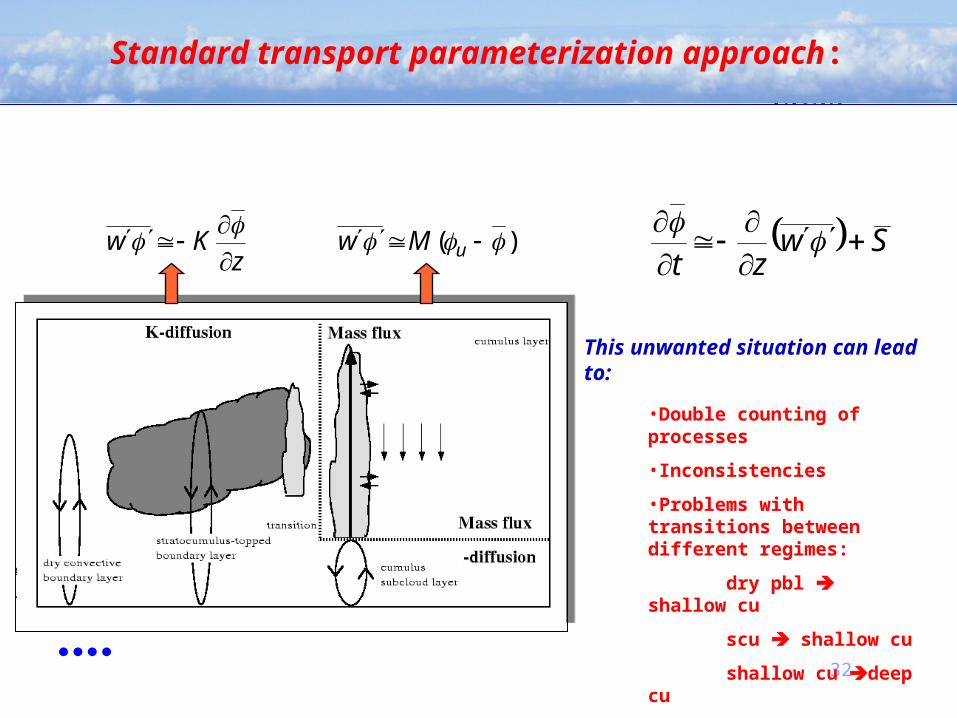
•Double counting of processes

•Inconsistencies

•Problems with transitions between different regimes:

dry pbl shallow cu

scu shallow cu

shallow cu deep cu

This unwanted situation can lead to:

Swzt

zKw

)( uMw

Standard transport parameterization approach:

vvcc

tcc

gBaBwb

z

w

z

M

M

qz

0

22

l

,2

1

1

,for)(

vvcc

tcc

gBaBwb

z

w

z

M

M

qz

0

22

l

,2

1

1

,for)(

M

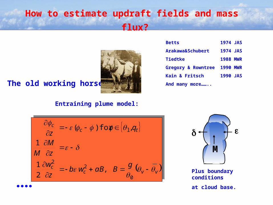
The old working horse:

Entraining plume model:

Plus boundary conditions

at cloud base.

How to estimate updraft fields and mass

flux? Betts 1974 JAS

Arakawa&Schubert 1974 JAS

Tiedtke 1988 MWR

Gregory & Rowntree 1990 MWR

Kain & Fritsch 1990 JAS

And many more……..

34

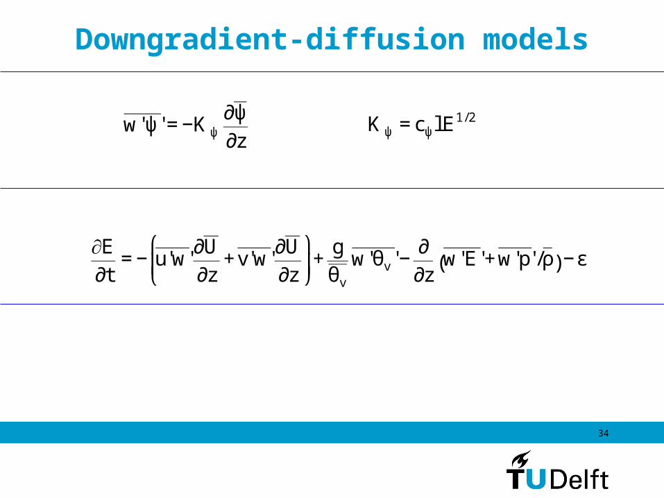
Downgradient-diffusion models

€

∂E∂t

= − u' w'∂U∂z

+v' w'∂U∂z

⎛

⎝ ⎜

⎞

⎠ ⎟+

gθv

w' θv ' −∂∂z

w' E' +w' p' /ρ( ) −ε

€

w' ψ' = −Kψ∂ψ∂z

€

Kψ = cψl E1/2

35

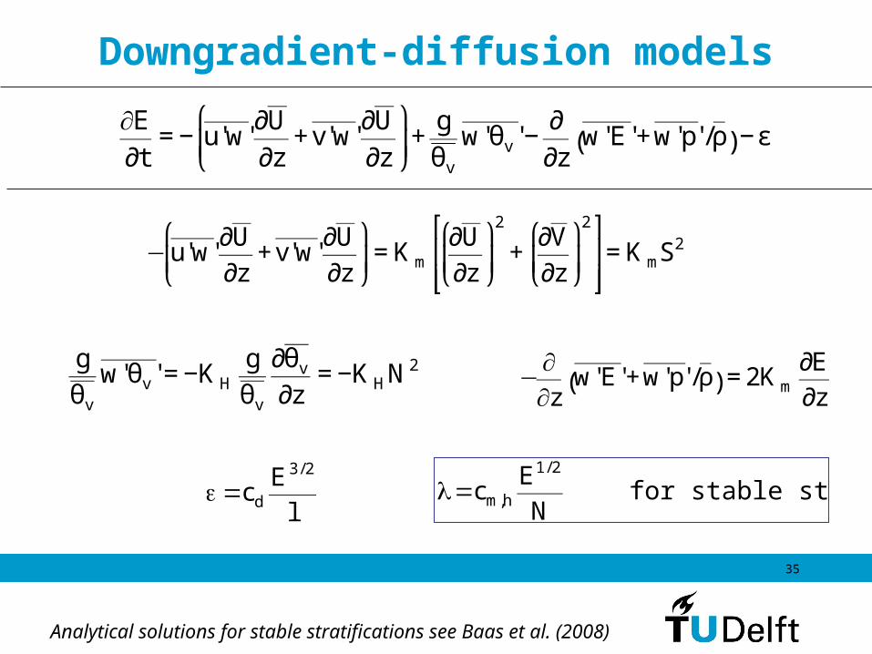
Downgradient-diffusion models

€

∂E∂t

= − u' w'∂U∂z

+v' w'∂U∂z

⎛

⎝ ⎜

⎞

⎠ ⎟+

gθv

w' θv ' −∂∂z

w' E' +w' p' /ρ( ) −ε

€

−u' w'∂U∂z

+v' w'∂U∂z

⎛

⎝ ⎜

⎞

⎠ ⎟= Km

∂U∂z

⎛

⎝ ⎜

⎞

⎠ ⎟

2

+∂V∂z

⎛

⎝ ⎜

⎞

⎠ ⎟

2 ⎡

⎣ ⎢ ⎢

⎤

⎦ ⎥ ⎥= KmS2

€

gθv

w' θv ' = −KHgθv

∂θv

∂z= −KHN2

€

−∂∂z

w' E' +w' p' /ρ( ) = 2Km∂E∂z

€

=cdE 3/2

l

€

l =cm,hE1/2

N for stable stratification

Analytical solutions for stable stratifications see Baas et al. (2008)

36

Stable boundary layer solutions

Nie

uwst

adt's

(19

84)

z/

∞

37

Turbulence and clouds: do we care?

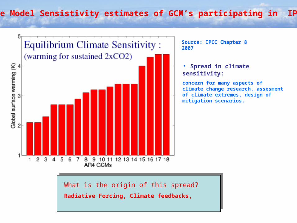
Climate Model Sensistivity estimates of GCM’s participating in IPCC AR4

Source: IPCC Chapter 8 2007

• Spread in climate sensitivity:

concern for many aspects of climate change research, assesment of climate extremes, design of mitigation scenarios.

What is the origin of this spread?

Radiative Forcing, Climate feedbacks,

Relative Contributions to the uncertainty in climate feedbacks

Source: Dufresne & Bony, Journal of Climate 2008

Radiative effects only

Water vapor feedback

Surface albedo feedback

Cloud feedback

Uncertainty in climate sensitivity mainly due to (low) cloud feedbacks