Embed Size (px)
Citation preview

1ANALISIS TRIWULANAN: Perkembangan Moneter, Perbankan dan Sistem Pembayaran, Triwulan II - 2007
BULLETIN OF MONETARY ECONOMICS AND BANKING
Department of Economic Research and Monetary PolicyBank Indonesia
PatronPatronPatronPatronPatronDewan Gubernur Bank Indonesia
Editorial BoardEditorial BoardEditorial BoardEditorial BoardEditorial BoardProf. Dr. Anwar Nasution
Prof. Dr. Miranda S. GoeltomProf. Dr. Insukindro
Prof. Dr. Iwan Jaya AzisProf. Iftekhar HasanDr. M. Syamsuddin
Dr. Perry WarjiyoProf. Masaaki Komatsu
Dr. Iskandar SimorangkirDr. Solikin M. JuhroDr. Haris Munandar
Dr. Andi M. Alfian ParewangiM. Edhie Purnawan, SE, MA, PhD
Dr. Buhanuddin Abdullah, MA
Editorial ChairmanEditorial ChairmanEditorial ChairmanEditorial ChairmanEditorial ChairmanDr. Perry Warjiyo
Dr. Iskandar Simorangkir
Executive DirectorExecutive DirectorExecutive DirectorExecutive DirectorExecutive DirectorDr. Andi M. Alfian Parewangi
SecretariatSecretariatSecretariatSecretariatSecretariatArifin M. Suriahaminata, MBA
Rita Krisdiana, S.Kom, ME
The Bulletin of Monetary Economics and Banking (BEMP) is a quarterly accredited journalpublished by Department of Economic Research and Monetary Policy Bank Indonesia. Theviews expressed in this publication are those of the author(s) and do not necessarily reflectthose of Bank Indonesia.
We invite academician and practitioners to write on this journal. Please submit your paper andsend it via mail to: [email protected]. See the writing guidance on the back of thisbook.
This journal is published on; January – April – August – October. The digital version includingall back issues are available online; please visit our link: –http://www.bi.go.id/web/id/Publikasi/Jurnal+Ekonomi/. If you are interested to subscribe for printed version, please contact ourdistribution department: Publication and Administration Section – Department of Economyand Monetary Statistics, Bank Indonesia, Building Sjafruddin Prawiranegara, 2nd Floor - Jl. M.H. Thamrin No.2 Central Jakarta, Indonesia, Ph. (021) 2310108 / 2310408 ext. 4119, fax.(021) 3802283, email: [email protected].

BULLETIN OF MONETARY ECONOMICSAND BANKING
Volume 15, Number 2, October 2012
QUARTERLY ANALYSIS: The Progress of Monetary, Banking and Payment System,
Quarter III - 2012
Author Team of Quarterly Report, Bank Indonesia
Optimal Credit Growth
G.A Diah Utari, Trinil Arimurti, Ina Nurmalia Kurniati
Global Financial Crises and Economic Growth : Evidence from East Asian Economies
Arisyi F. Raz, Tamarind P. K. Indra, Dea K. Artikasih, and Syalinda Citra
The Dynamics Spillover of Trade between Indonesia and Its Counterparts in Terms
of AFTA 2015 : A Modified Gravity Equation Approach
Barli Suryanta
Impact of Global Financial Shock to International Bank Lending in Indonesia
Tumpak Silalahi, Wahyu Ari Wibowo, Linda Nurliana
3
55
1
35
75

1ANALISIS TRIWULANAN: Perkembangan Moneter, Perbankan dan Sistem Pembayaran, Triwulan II - 2007

1QUARTERLY ANALYSIS: The Progress of Monetary, Banking and Payment System Quarter III – 2012
QUARTERLY ANALYSIS:The Progress of Monetary, Banking and Payment System
Quarter III – 2012
Author Team of Quarterly Report, Bank Indonesia
The domestic economy is still growing quite well despite a slight slowdown. Indonesia’s
economic growth in the third quarter of 2012 grew by 6.2%, slightly lower than previous
forecasts due to a continuing decline in the performance of the external sector. Although
consumption and domestic-orientated investment demand remains high, falling exports have
resulted in decreased production and export-oriented investment. Looking ahead, economic
growth is expected to rise again, driven by domestic consumption and investment which remainsstrong. Exports are predicted to also improve in line with the improving economy with some
major trading partners, though it will still be shadowed by uncertainties in the global economic
conditions. With these developments in the Indonesian economy for the entire year of 2012,
the economy in 2013 is forecasted to grow 6.3% in rising into the range of 6.3% -6.7%.
Indonesia’s balance of payments (BOP) in the third quarter 2012 is forecasted at a surplus,
supported by an improved and greater current account surplus in the capital and financialaccounts. The current account deficit in the third quarter 2012 was lower than expected
compared to second quarter 2012. This was indicated in August 2012 when the trade balance
recorded a surplus. On the other hand, the capital and financial accounts surplus were expected
to increase along with capital inflows and a substantial portfolio inflow of foreign direct
investment (Foreign Direct Investment / FDI) that remained high. As a result, the amount of
reserves at the end of September 2012 increased compared to the end of the previous month,reaching U.S.D 110.2 billion, equivalent to 6.1 months of imports and government foreign
debt payments.
The exchange rate in September 2012 moved according to market conditions with an
intensity that decreased with depreciation. This is in line with the policy adopted by Bank
Indonesia to stabilize the exchange rate in accordance with the fundamental levels. The Rupiah
point-to-point weakened by 0.37% (mtm) to Rp9,570 to the U.S. dollar, or on average weakened
by 0.64% (mtm) to Rp9,554 to the U.S. dollar. Pressure on the exchange rate came mainlyfrom the high demand for foreign exchange from import demands. Pressure on the rupiah
dropped due to the greater inflow of foreign capital in line with a positive sentiment in the
global economy and the outlook for a strong domestic economy.

2 Bulletin of Monetary, Economics and Banking, October 2012
Inflationary pressure tended to decrease and be controlled at a low level. CPI inflation in
September 2012 was 0.01% (mtm) resulting in an annual rate of 4.31% (yoy). Core inflation
was at the lowest level at 4.12% (yoy), in line with an easing post-holiday demand, a correction
in global commodity prices, and controlled expectations. Food inflation (food volatility) also
decreased, driven by significant lower prices of food commodities, and a sustained supply and
hardline policy adopted by the Government in controlling food prices. On the other hand,inflation on administered prices was also controlled in the absence of government policy on
the prices of strategic goods and services.
In line with the macroeconomic performance that was maintained, the stability of the
financial system and banking intermediation function were properly maintained. Solid industry
performance was reflected in the high capital adequacy ratio (CAR), which was well above the
minimum 8% and the maintained ratio of gross non-performing loans (NPL) under 5%.
Meanwhile, credit growth to the end of August 2012 reached 23.6% (yoy), which was downfrom 25.2% (yoy) of the previous month. The slowdown was mainly on working capital loans
that grew by 23.2% (yoy), while consumer loans had relatively stable growth at 19.9% (yoy).
Investment credit growth was quite high, at 29.8% (yoy), and is expected to increase the
capacity of the national economy.
Solid economic performance in Indonesia cannot be separated from the support of a
reliable payment system. In economic activities, the strategic role of the payment system is toensure the implementation of various payment transactions of economic activity and other
activities undertaken by both the public and the private sectors. During the third quarter of
2012, the payment system demonstrated a positive performance. The value of the payment
system and the transaction volume during the quarter remained relatively robust in 2012 in
line with the solid economic activity. In addition, the payment system transactions increased
and were also supported by Bank Indonesia’s policy directed to ensure the implementation ofan efficient, fast, secure, and reliable payment system. On the other hand, the circulation of
money, currency outside banks as a means of payment, still played an important role in the
society. This is reflected in the high growth of currency in circulation (UYD) during the third
quarter of 2012 along with the growth of economic activity that remains solid.
3Optimal Credit Growth
OPTIMAL CREDIT GROWTH
G.A Diah Utari, Trinil Arimurti, Ina Nurmalia Kurniati1
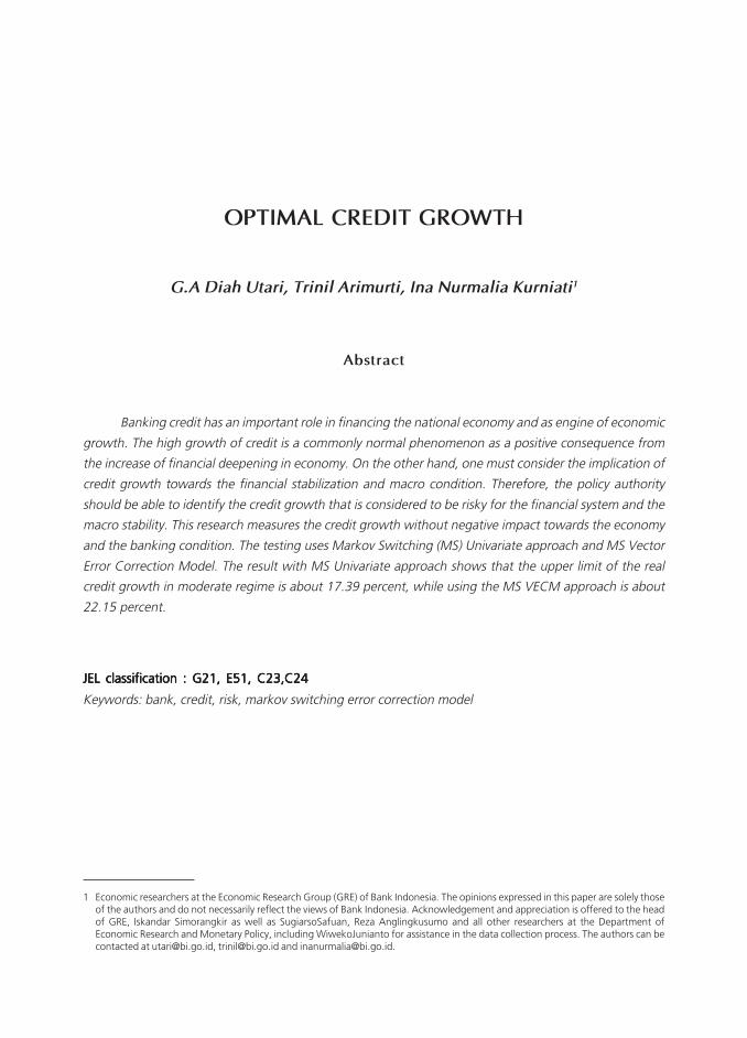
Banking credit has an important role in financing the national economy and as engine of economic
growth. The high growth of credit is a commonly normal phenomenon as a positive consequence from
the increase of financial deepening in economy. On the other hand, one must consider the implication of
credit growth towards the financial stabilization and macro condition. Therefore, the policy authority
should be able to identify the credit growth that is considered to be risky for the financial system and the
macro stability. This research measures the credit growth without negative impact towards the economy
and the banking condition. The testing uses Markov Switching (MS) Univariate approach and MS Vector
Error Correction Model. The result with MS Univariate approach shows that the upper limit of the real
credit growth in moderate regime is about 17.39 percent, while using the MS VECM approach is about
22.15 percent.
Abstract
JEL classification : G21, E51, C23,C24JEL classification : G21, E51, C23,C24JEL classification : G21, E51, C23,C24JEL classification : G21, E51, C23,C24JEL classification : G21, E51, C23,C24
Keywords: bank, credit, risk, markov switching error correction model
1 Economic researchers at the Economic Research Group (GRE) of Bank Indonesia. The opinions expressed in this paper are solely thoseof the authors and do not necessarily reflect the views of Bank Indonesia. Acknowledgement and appreciation is offered to the headof GRE, Iskandar Simorangkir as well as SugiarsoSafuan, Reza Anglingkusumo and all other researchers at the Department ofEconomic Research and Monetary Policy, including WiwekoJunianto for assistance in the data collection process. The authors can becontacted at [email protected], [email protected] and [email protected].
4 Bulletin of Monetary, Economics and Banking, October 2012
I. INTRODUCTION
Banking credit has an important role in financing national economy and as the engine of
the economic growth. The availability of credit enable households to consume more and enable
company to invest which they cannot afford using their own fund. Besides, in the presence of
moral hazard and adverse selection problems, which occurs commonly, the bank plays important
role in capital allocation and supervision to ensure that public fund will be distributed to themost optimal benefited activities. Regardless the increasing financing role through capital market
and bank and financing company, the banking credit still dominates the total credit to private
sector with the average of 85%2.
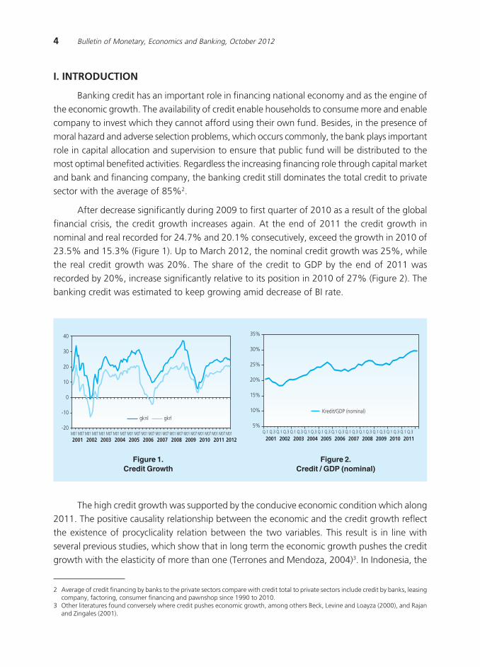
After decrease significantly during 2009 to first quarter of 2010 as a result of the global
financial crisis, the credit growth increases again. At the end of 2011 the credit growth in
nominal and real recorded for 24.7% and 20.1% consecutively, exceed the growth in 2010 of23.5% and 15.3% (Figure 1). Up to March 2012, the nominal credit growth was 25%, while
the real credit growth was 20%. The share of the credit to GDP by the end of 2011 was
recorded by 20%, increase significantly relative to its position in 2010 of 27% (Figure 2). The
banking credit was estimated to keep growing amid decrease of BI rate.
2 Average of credit financing by banks to the private sectors compare with credit total to private sectors include credit by banks, leasingcompany, factoring, consumer financing and pawnshop since 1990 to 2010.
3 Other literatures found conversely where credit pushes economic growth, among others Beck, Levine and Loayza (2000), and Rajanand Zingales (2001).
Figure 1.Credit Growth
Figure 2.Credit / GDP (nominal)
The high credit growth was supported by the conducive economic condition which along2011. The positive causality relationship between the economic and the credit growth reflect
the existence of procyclicality relation between the two variables. This result is in line with
several previous studies, which show that in long term the economic growth pushes the credit
growth with the elasticity of more than one (Terrones and Mendoza, 2004)3. In Indonesia, the
���� ����
��
�
�
�
�
� � � � � � � � � � � ���� ���� ���� ���� ���� ���� ��� ��� ���� ���� ���� ����
��
�
��
��
���
��
���
��������������������
���� ���� ���� ���� ���� ���� ��� ��� ���� ���� ���� ! !� ! !� ! !� ! !� ! !� ! !� ! !� ! !� ! !� ! !� ! !�

5Optimal Credit Growth
causality relationship tends to show the dominant role of the economic growths as the lead
variable, rather than the credit growth ((Nugroho and Prasmuko (2010) and Utari et.al. (2011)).
On one hand, the rapid credit growth is a normal phenomenon and is a positive
consequence from the increase of financial deepening in economy. On the other hand however,
this credit growth has direct implication to the financial stability and the macro condition
particularly when the rapid credit growth is followed by a weakening current account and
vulnerable financial sector. This leads to the question of what is the rate of credit growthconsidered to be conducive for the economic growth and will not create pressure toward the
inflation and the banking micro condition. The assessment for the credit growth is not only
related to the amount distributed, but also its sectoral distribution.
According to several literatures, excessive credit growth can threaten the macroeconomic
stability. The increase of credit especially consumptive one may trigger the growth of aggregate
demand higher than the potential output which causes the economics to overheat. This in turnwill increase of inflation, current accountdeficit as well as exchange rate appreciation.
Simultaneously, during expansion period, the banking institution tends to have over optimistic
expectation on the ability of the customer to pay, hence is careless in allocating credit for the
high risk group. This type of credit will accumulate and potentially turn to be a bad loan during
the economic contraction period.
The lesson learned from the earlier global financial crisis was the importance of the policyauthority in supervising the risk from excess credit distribution. This is because the excessive
aggregate credit is often related to the systemic risk. Therefore the policy authority is advised
to identify the level of credit growth which is considered to be risky for financial system and
macro stabilization. Another important thing is the countercyclical macroprudential policy to
anticipate the risk from excessive of credit growth. Maintaining the financial system stability
particularly for the bankingsector in this context is not only to ensure the banking sector bothin aggregate or individually, to have good solvency during the period of distress, but also to
have sufficient capital in keeping the allocation of the credit for the economy.
Based on the considerations above, the purposes of this research is to calculate the level
of credit growth that is considered not to have negative impact on the economy and the
banking condition. The presentation of this paper is as follows; the next session discusses the
literature review on basic theory related to the credit, the financial and macro stability as well
as the credit threshold. The third session will elaborate the development of credit in Indonesia.Methodology and data is presented in session four, while session five explains the empirical
result. The conclusion and recommendation will close the presentation of this paper.

6 Bulletin of Monetary, Economics and Banking, October 2012
II. LITERATURE REVIEW
2.1. Credit Growth, Financial System Stability and Macro Stability
The episodes of rapid credit growth – “credit boom” – posed a policy dilemma. Creditboom is defined as: 1) a period when there was a fairly extreme deviation from the credit
growth to its long-term historical pattern that was not supported by the fundamentals (Iosifovand Khamis, 2009) and 2) an episode when credit growth to the private sector exceeded
growth in a normal business cycle (Mendoza and Terrones, 2008). More credit means increasing
access to finance and greater support for investment and economic growth. But these conditions
may lead to the vulnerability of the financial sector through the loosening of lending standards,
excessive leverage and asset price bubbles (Reinhart and Rogoff, 2009.)
Rapid credit growth could be triggered by several factors (Dell’Ariccia, et al, 2012): 1)
part of the normal phase of a business cycle, 2) financial liberalizations and 3) surges in capitalinflows. As explainedin the Dell Ariccia (2012), under normal conditions, as domestic economic
improve, the credit will generally grow faster. This is generated by the firm’s investment needs
both in the form of new investment and capacity expansion. Rapid credit growth is also generated
by financial liberalizations, which is initially intended to foster the financial deepening. Another
factor contributing to credit growth is the capital inflows. It will increase in the funds available
to banks, then eventually increasing credit growth. Unlike the first three, credit growth generatedby an excessive response of the financial sector agents will lead to excessive credit growth
(credit boom). This condition is based on theory of financial accelerator4. It is found as the
market imperfection due to asymmetric information and weak institutional. Besides three factors
above, Terrones (2011) also suggests other factors are excessive response from financial sector
agents due to changes in risk over time.
In some literature, excessive credit growth is often attributed as a key factor contributingto the crisis in the financial sector, particularly in emerging countries. Credit booms had also
preceded many of the largest banking crises of the past 30 years: Chile (1982), Denmark,
Finland, Norway and Sweden in 1990/91, Mexico (1994) Thailand and Indonesia (1997/98)
(Dell Aricia, et al, 2012). Kaminsky, Lizondo and Reinhart (1997) found that five of the seven
studies surveyed prove credit growth is one determinant of the financial or banking crisis. Craig
et al (2006) and Hardy and Pazarbasiouglu (1998) in Craig et al (2006) found that deteriorationin business cycle and crisis in emerging markets are commonly preceded by a period of rapid
credit growth and asset price bubbles. Similar results were also obtained from the study Goldstein
(2001), IMF (2004a) and Mendoza and Terrones (2008). Goldstein (2001) proved the relation
between the credit boom and the possibility of a twin crisis (financial and banking crisis). IMF
found that three-fourth of the period of credit boom in the sample of emerging countries is
associated with the banking crisis, while seven-eighths is associated with the financial crisis.
4 Financialacceleratorisa mechanism whichthe development ofthe financialsectormay affectthe business cycle (Fischer, 1933 in Penettaand Angelini, 2009).

7Optimal Credit Growth
Meanwhile, Mendoza and Terrones (2008) found that for emerging markets, approximately
68% of the boom sare associated with foreign exchangecrises, 55% withbanking crises, and32%withsudden stops.
A significant expansion in credit growth generally will increase the vulnerability of the
financial system. This condition is driven by the behavior of banks which tend to be pro cyclical.
The pro-cyclicality characteristic of the banking sector through their lending is an element of
the systemic risks that need to be highly considered by the authorities. There fore, one goal ofthe macroprudential policy is to create the incentives for the financial sector to be less pro-
cyclical (Gersl and Jakubic 2010 in Frait et al, 2011).
As shown in Figure 2 1 were explored in a paper Frait et al, (2011), during the expansion
phase, the aggregate demand will significantly increase, as well as the growth of bank lending
and the economic leverage. This condition is usually accompanied by an increase in corporate
profits, asset prices and consumer expectations. The surge in asset prices will increase collateralso that the new credit will be more easily administered and encourage banks and customers to
be more willing to take risks. In this phase, the accumulation of the risks will be materialized in
the case of the economic downturn. Increased household and corporate leverage/indebtedness
would increase the vulnerability to macroeconomic risk through excessive aggregate demand
growth beyond the capacity of the economy and eventually lead to overheating pressures.
Bank credits boost the consumption and imports with the subsequent effect in increasingcurrent account deficit. The worsening sustainable current account deficit may lead to the
reduction of the capital inflows and eventually affects the financial and banking sector health.
This is possible since the market will reacts to the increased of macroeconomic conditions risk
by adjusting their portfolio investment, including the ownership of the currencies.
Meanwhile, in terms of microeconomic views, higher debt stock put the borrowers exposed
with interest rate and exchange rate risk (if credit is distributed in foreign currency). Withouthedging the exposure, the vulnerability of the debtor to both risks would increase the credit
risk. The increasing in debt payments due to the rising of interest rates or the currency
depreciation may lead to serious implications for the credit portfolio of the bank and for the
real economic activity. The household and the firm’s budget will be allocated more to
accommodate the rising of the debt burden. After the peak of the boom cycle ends, the
company’s profit decline and credit worthiness also decreased. Finally, this will increase thenon-performing credits, and eventually affects the health of bank balance sheets.
Vulnerability in balance sheet of the banking, the financial system and the macroeconomic
is related each other. The macroeconomic imbalances reflected in the sudden changes in
interest rates and exchange rates may affect the debtor’s ability to repay debt and at the same
time raises concerns about the health of the financial sector. For example, sudden reversal
capital inflow could lead to a hard landing in the economy and force the authorities to raise
interest rates. These conditions will further put pressure on the banking sector through the

8 Bulletin of Monetary, Economics and Banking, October 2012
credit risk resulting from an increase in interest rates, economic slowdown and declining of
collateral value. On the other hand, concerns about the financial sector will encourage the
macroeconomic instability due to market reaction.
Figure 3.Financial Cycle and Systemic Risk Evolution
2.2. Identification of Excessive Credit
One way to identify the presence of excessive credit growth is to compare the credit
growth within the same economic group levels. The credit to GDP ratio is widely used as a
benchmark for the ability to repay. Therefore, countries with the same stage of the economy
should have the same level of credit balance. Countries with low levels of the economy stage
will naturally have a lower level of credit compared to the more developed countries. We can
identify the credit threshold in the country by analyzing the trend of the credit to GDP ratiofrom countries within similar level of economic stage.
Another approach to identify the presence of the excess credit growth is the HP filter
method. The trend estimated from HP Filter is regarded as equilibrium and the credit boom is
defined as credit that exceeds a certain threshold around this trend. Threshold values can be
defined as the relative deviation from the trend as used by Gourinchas et al. (2001) and IMF
(2004). Nakornthab et al. (2003) have analyzed the trend component of the credit-to-GDP
ratio with the estimate period 1951-2002. The main criticism of the methods of the HP filterthat use only size of credit solely and do not take into account for the economic fundamentals
that affect the balance of the credit stock.
Estimated credit equilibrium using fundamental economic variables are the most commonly
used approach. Hofmann (2001) estimated the equilibrium level of credit to GDP ratio with
"�#�$�%�&���������������
�������� �������������� �����������������
'�������(�����������)������*�(+(����$���(��%�,-�(���*����.��������/��-�0$�((�.��,�((���(�
��1��������.��������.��
���������(���$$#�#�������*�(+(����$���(��%�,-�(���*��$���(������.������/��-�0$�((�.���,����(�
"����������$��.������$��,�#�������,���$+%�*��/����������������$����(�$��������,2�,��,���+�,��$����,!���$�
��($�����#�#(�$-������������������(���*�*����$����(��3����+%��!�!*����$���������������$����(��$�����(,����(2�4�"�(,����(�������������5#����+�����$����(
"�������������(#,,����,���$��(%$#����������$����(����*�#�������21�6������2�,��.�(�����������2��������$��������(������*����$��������������$����(

9Optimal Credit Growth
VECM model. Boyssay et al. (2005) applied the model ECM and panel of credit data from
Central and Eastern Europe countries. Backe et al (2005) estimated a panel model ECM on a
combination of several OECD and emerging countries. Eller et al (2010) used VECM and estimated
the long-term equation which is the demand side credit and short-term equation is the supply
side of the credit. Short-term dynamics are modeled by Markov switching error correction that
allows the credit coefficient varies according to its regime. Egert et al (2006) in Kelly et al(2011) using the panel out-of-sample to estimate the balance of credit in countries with transition
economies.
III. METHODOLOGY AND DATA
This paper will analyze the excessive credit by using HP Filter. In addition we also use the
equilibrium approach of the credit demand and supply, using fundamental variables, which is
estimated using Markov Switching Vector Error Correction Model (MSVECM). Both approachesrely on information in the past.
3.1. HP Filter Analysis
As mentioned in the previous chapter, one of the methods to identify the presence of
excess credit growth is the Hodrick Prescott filter (HP filter) approach. HP filter introduced by
Hodrick and Prescott (1980), is a flexible detrending method and is commonly used in economicresearch.
Suppose a data series yt can be separated into 2 components, namely trend (gt) and cycle
(ct) and written as yt=gt+ ct. HP Filter method to separate components of the cycle by solving
the following optimization of the loss function, which is also known as the two sides HP filter
approach:
(1)
where λ (lambda) is the smoothing parameter. The first term of equation (1) measure
the accuracy of the model, or in other words the penalty for the variance of the cyclical
component. The second term is penalty of smoothness level of the trend. Therefore there is a
conflict between a smoothness trend and its good ness of fit, where λ is the “trade off”
parameter that can be . If λ is zero then the trend component will be equal to the original data,
and if it is infinite, , then the trend will converge to the linier trend (gt=β * t).
Hodrick and Prescott suggest λ=1600 for quarterly data, and is the standard for business
cycle analysis. Value of λ assumes the business cyclehas a frequency of approxi matel y 7.5
years. Ravnand Uhlig (2002) from Drehman and Borioet al (2010) showedthat the value of λ

10 Bulletin of Monetary, Economics and Banking, October 2012
should be adjusted if the frequency of data changes. Convention researchers proposed value
λ=100 forannual data, λ= 1600 for quarterly data, and λ=14,400 for monthly data.
Undeniably, the HP filter method also has some disadvantagesas proposed by Cottarellietal.
(2005); first the HP filter measure the trend of the overall observations and ignores the possibility
of a structural break; second, the HP filter is sensitiveto the bias of the tip point. If the start or
the end pointof the data does notreflectthe same thing inthecycle, then it tends tobiasupward
/downward; third, the HPfilteris sensitive to the selection of time duration. Gourichasetal (2001)conducted a rolling HP filter and found that the HP filter estimation resultscan bevery different
from theex-post trend estimation and, fourth, the HP filter sensitive to the smoot hingpara
meter (λ) used.
Inthis paper, the excessive credit growth will be analyzed by looking at the deviation of
the long-term trend (using HP filter) to the credit growth, and also credit-to-GDP ratioand its
deviation from the long-term trend. Usingthe ratio of credit to GDP is following theapproachproposed by the Basel Committee on Banking Supervision (2010). Following the IMF (2004),
the thre shold level used is 1 and 1.75 times standard deviation of thelong-term trend.
3.2. MSVAR
Markov Switching (MS) model from Hamilton (1989), also known by the model of regime
switching is one of the popular non-linear time series model. This model contains several
structures (equations) which describe the characteristics of time series data in different regimes.By doing switching between the structures, the model is expected to capture a more complex
dynamics. The main feature of MS is switching mechanism controlled by unobservable state
variable that follows Markov chain of order 1. In general, the general nature of Markov is that
the present value is affected by the value of the past. MS may explain the correlated data
showing the dynamic pattern at some period of time. MS model has been widely applied to
analyze time series data and financial economics.
MS-VAR model provides a framework for analyzing multivariate (and univariate)representation, in the presence of regime switching. MS-VAR model is a dynamic structure
that depends on the value of the state variable (St), which controls the switching mechanism
between some state (regime). A common form of MS-VAR models are:
������������ ������������� ������ ��������������� � ������������������������������ ��������������� ������������������ �������������
������������ ��� ����� ����� � ����������������
� ������� ���������� ! "�����# $��%&&'�"#�%&'%� �������� ��(��������) ! �*������# *'�%&&'�*'�%&'%
������������ ����������������
11Optimal Credit Growth
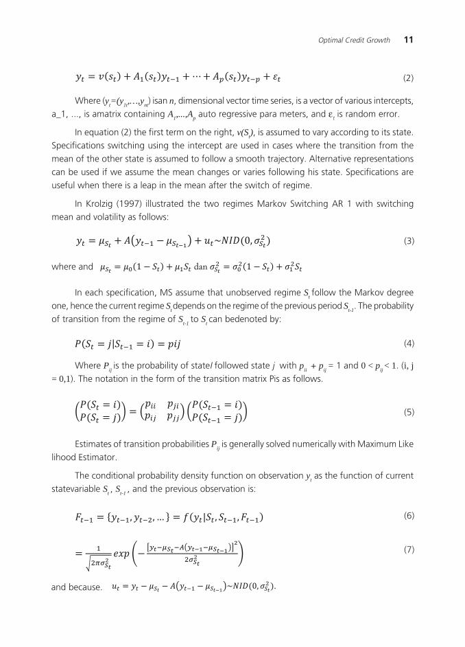
Where (yt=(y1t,…,ynt) isan n, dimensional vector time series, is a vector of various intercepts,
a_1, ..., is amatrix containing A1,...,Ap auto regressive para meters, and εt is random error.
In equation (2) the first term on the right, v(St), is assumed to vary according to its state.
Specifications switching using the intercept are used in cases where the transition from the
mean of the other state is assumed to follow a smooth trajectory. Alternative representations
can be used if we assume the mean changes or varies following his state. Specifications are
useful when there is a leap in the mean after the switch of regime.
In Krolzig (1997) illustrated the two regimes Markov Switching AR 1 with switching
mean and volatility as follows:
(2)
In each specification, MS assume that unobserved regime St follow the Markov degree
one, hence the current regime St depends on the regime of the previous period St-1. The probability
of transition from the regime of St-1 to St can bedenoted by:
(3)
dan where and
(4)
Where Pij is the probability of stateI followed state j with pii + pij = 1 and 0 < pij < 1. (i, j= 0,1). The notation in the form of the transition matrix Pis as follows.
(5)
Estimates of transition probabilities Pij is generally solved numerically with Maximum Like
lihood Estimator.
The conditional probability density function on observation yt as the function of current
statevariable St , St-1 , and the previous observation is:
(6)
(7)
. and because.
12 Bulletin of Monetary, Economics and Banking, October 2012
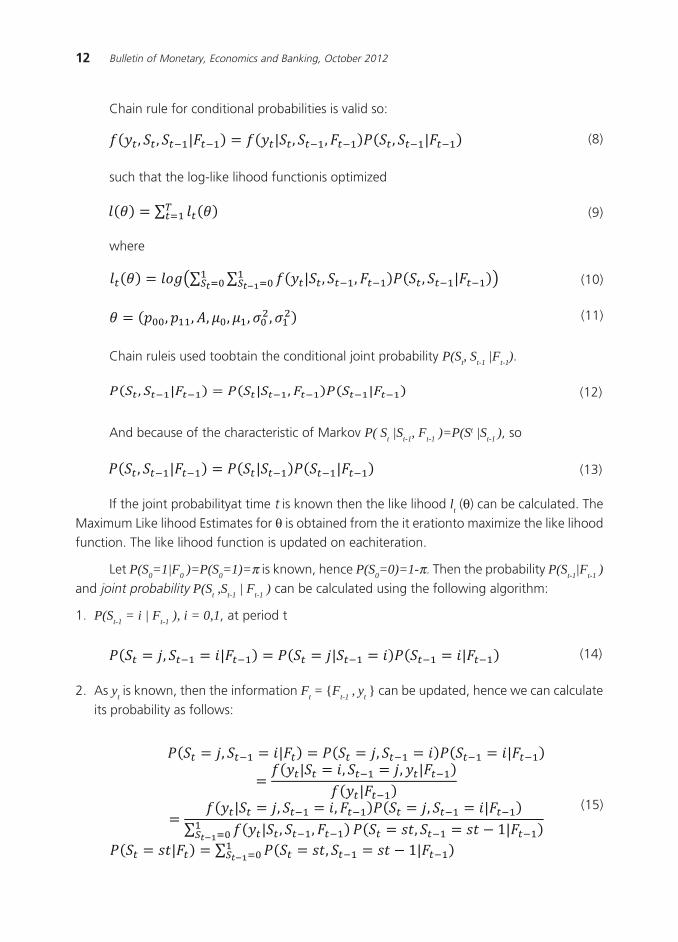
Chain rule for conditional probabilities is valid so:
where
(8)
If the joint probabilityat time t is known then the like lihood lt (θ) can be calculated. The
Maximum Like lihood Estimates for θ is obtained from the it erationto maximize the like lihoodfunction. The like lihood function is updated on eachiteration.
Let P(S0=1|F0 )=P(S0=1)=π is known, hence P(S0=0)=1-π. Then the probability P(St-1|Ft-1 )and joint probability P(St ,St-1 | Ft-1 ) can be calculated using the following algorithm:
1. P(St-1 = i | Ft-1 ), i = 0,1, at period t
(9)
(10)
(11)
(12)
(14)
(15)
such that the log-like lihood functionis optimized
Chain ruleis used toobtain the conditional joint probability P(St, St-1 |Ft-1).
And because of the characteristic of Markov P( St |St-1, Ft-1 )=P(St |St-1 ), so
(13)
2. As yt is known, then the information Ft = {Ft-1 , yt } can be updated, hence we can calculate
its probability as follows:

13Optimal Credit Growth
Probability of Steady state : P(S0 = 1, | F0 ) and P(S0 = 0, | F0 )
(16) dan .and
The data used in this studyis the monthly real credit data from January 2003 to March
2012. This period waschosen to eliminate the impact of the Asian crisis. The data sourceis from
Bank Indonesia.
3.3. MS VECM
In this research, empirically weal so test the credit thre shold using multivariate analysis
that takes into account the variable of the demand and the supply of credit. From this empiricalanalysis, wewill also analyze the determinants of changesin credit, both in the short and in the
long-term.
MSVECM Analysis consists of 2 stages namely the analysis Vector Error Correction Model
(VECM) followed by the analysis of Markov Switching. VECMVAR model is designed for useina
data series that is not stationary and is known to have acointegration relationship. InVECM,
there are specifications that limit the long-term behavior of the endogenous and exogenousvariables to converge to its cointegration relations hipsbut allow dynamic adjustments in the
short term. In cointegration, there is error correction term, since the deviation from the long-
term equilibriumis gradually corrected through the short-term adjustment. MS-VECM is actually
a VECM with shif tingpara meters. Following Krolzig (1997), VECMfor variables I (1)can be
mode ledinto
(17)
where Δxt is a vector of dimensionless variables m, v(St)= is the regime dependent intercept
Γi, is matrix of parameters and error variance is allowed to change over regime ut ~ (0, Σ(st)).In this term, α(st) is the matrix of adjustment parameters, and β is the matrix of long-term
parameters (co-integration vectors).
Steps undertaken in the VECM analysis can be displayed in the following chart:
� ����������
� ������������
����������������
� ������� ���������!������"#������$�� ��%&

14 Bulletin of Monetary, Economics and Banking, October 2012
Before applying the co-integration test, we need to do some preliminary testing. First,
the optimal lag test was done to overcome the problem of autocorrelation and heteroscedasticity
(Gujarati, 2003). Determination of the optimal lag is important because when the lag is too
long will reduce the degrees of freedom, while the too short lag will result in an incorrect
specification model (Gujarati, 2003). The determination of optimal lag is based on five criteria,
namely the sequential modified LR test statistic, Akaike Information Criterion (AIC), SchwarzInformation Criterion (SC), Final Prediction Error (FPE), and Hannan-Quin Information (HQ).
From these criteria, we will use the criterion that gives the shortest lag. Further tests carried out
in the form of residual correlogram. VAR system of equations passes the test if the correlation
between the lag and the variables are within the specified range.
After making various preliminary tests, the co-integration test can be performed. If it
found co-integration vector, weak exogeneity test would then perform to ensure the long-
term causality and to check whether there is feedback from the short-term variables to thedependent variable. Weak exogeneity of each variable is done by restricting α_i = 0, where αis a vector of adjustment coefficients and i = 1,2,3. If the zero restriction is not rejected, it
means the variable has no feedback to the past deviations from long-term relationships (weakly
exogenous).
Meanwhile, the existence of co-integration relationship does not necessarily mean that
the equilibrium exist in the model. Co-integration is able to capture the long-term relationshipbetween dependent and explanatory variables, however it cannot capture how the dynamic
response of the dependent variable due to the changes in the explanatory variables. To capture
the response, we use the error correction framework, which is Vector Error Correction Model
(VECM). The short-term models that contain error correctionterm show how the adjustment
mechanism to return to equilibrium when the dependent variable is disturbed by the exogenous
shock. After conducting co-integration and weak exogeneity test, VECM estimation performedby the following equation:
(18)
where ECT is the error correction term derived from the co-integration vector; δ error
correction coefficient which shows the response of dependent variable in each period t. In
other words, δ shows the speed of adjustment back to its equilibrium and has to be negativeand significant, and no larger than one. In the case of disequilibrium, the negative value indicates
the correction process. Meanwhile, the low value of δ closed to zero means that the dynamic
effects dominate the behavior of the credit growth in the short term. Instead, if δ is larger and
closed to one then the long-term effects dominate the behavior of credit growth in the short
term, or simply the short-term dynamics has a small effect on the growth of credit.
Based on the linear VECM estimation, analysis is continued to estimate the MS- VECM
to examine the relationship between the variables that affect the demand for credit.

15Optimal Credit Growth
Long-Term Credit Equation: CointegrationLong-Term Credit Equation: CointegrationLong-Term Credit Equation: CointegrationLong-Term Credit Equation: CointegrationLong-Term Credit Equation: Cointegration
To analyze the behavioral changes of the optimal credit for the economy, both at macro
and micro level of banking, we adopt the model proposed by Psaradakis et al (2004), which is
also used by Eller et al (2010). We use the following framework: (i) the credit has a long-term
relationship with the fundamental macroeconomic variables (demand for credit) and in the
short term is influenced by banking micro variables (supply for credit), (ii) the adjustment of the
volume of credit on its equilibrium may not be linear because there is a period where the creditmarkets are in disequilibrium point, and the factors affecting the credit possibly change over
time.
Equation of demand for credit we use in this paper refers to the following model of Eller
et al (2010):
Where Krl is the total use of credit volume in real term after deflated with CPI, PDBrl isthe real GDP interpolatedin to monthly data, rt is mortgage interest rate (as a proxy for the
price of the credit), and πt is the annual CPI inflation .
(19)
Parameter for PDBrl is expected to be positive, showing the increasing economic activity
leads to the increase of demand for credit. Parameter value for variable r tis expected to benegative, showing higher credit interest rateswill reduce demand for credit since the costof
fundincrease. Parameters of π is also expectedto be negative, in line with the Elleretal (2010)
that negative relationship between inflation andcredit demand can be viewed from two aspects
: first, when the inflation has reacheda certain level, it will beassociated with inflation volatility
that significantly disturbs the function of financial markets due to the increase of uncertainty.
Second, if the nominalin terest rate is high, even real interest rate is low, the economic agentswill choose credit swith short duration, which in turn limitsthe volume of distributed credits.
������� ��� ����� ����� � ����������������
������� ���+,��- ! "�����# $��%&&.�"��%&'%
�)�����+) ��- ! "�����#�+!��������� - $��%&&.�"��%&'%
!�/������+���- ! "�����# $��%&&.�"��%&'%
!�������������/���� ���+�- ! "�����# $��%&&.�"��%&'%
������������ ��� �������������� �

16 Bulletin of Monetary, Economics and Banking, October 2012
EquationShort TermCreditsEquationShort TermCreditsEquationShort TermCreditsEquationShort TermCreditsEquationShort TermCredits
If the variables in the equation (20) have the cointegration relationship then we can
construct the following short-term dynamic error correction equation:
(20)
Where Δlog(Krlt ) is areal credit growth, εt-1 is the previous error correction term of the
long-term equation, β1 is the speed of adjustment parameter to the long-terme quation, and Zt
isset of other possible explanatory variables.
Vector Zt contains short-term determinants of the credits, consisting of third-party fundingand credit risk. Third party fund sare expected to havea positive relationship since the increase
of the available funds may also increase the distributed credit. For credit risk, we use the ratio
of Non-Performing Loan (NPL) to total assets. The expected relationship of this variable is
negative because the increasing non-performing loan leads to the decline of bank’s willing
ness to distribute the credit.
The above short-term equation is based on the assumption that the process of adjustmentto the equilibriumis with in the same regime. We can relax this assumption using MSVECM
framework by allowing parameters to change according to its unobservable state. Within the
framework of MSVECM above, the short-term equation can be transformed into:
where the short-term equation is conditional on theunobservable regime variable st.
IV. EMPIRICAL RESULTS
4.1. HP Filter Analysis
Analysis result using HP filter approach shows that the real growth of credit in Indonesiais still within the range of its long term trend either using the upper or the lower limit of 1
standard deviation or using the IMF standard of 1.75. We can observe that the real credit
growth until May 2012 by 20.7% remains in the long term range and relatively lower than the
credit growth in the end of 2008, which was closed to the upper limit (Figure 4). Looking at its
disaggregation, the growth of credit investment, working capital credit and consumption credit
remain in the long-term trend (Figure 5 up to Figure 7).
(21), for every st=1, 2, dst

17Optimal Credit Growth
However as explained by Cottarelli et al. (2005), one of the HP Filter weaknesses is
measuring the trend from overall observation and ignores the possible existence of structural
break. Considering this, we try to eliminate the data during the crisis, and sub sequently, the
HP Filter test is applied on the data for the period of January 2001 up to May 2011
Figure 4.Long Term Trend of Real Credit Growth
Figure 5.Long Term Trend of Real Investment Growth
Figure 6.Long Term Trend of Real Consumption Growth
Figure 7.Long Term Trend of Real Working Capital Growth
��� ��� ���� ���� ���� ���� ���� ���� ���� ���� ��� ��� ���� ���� ���� ���� 7 � � � � � 8 � 9 7 � � � � � 8 � 9 7 �
9
�
�
��
��
�9
�7
��:;;6 <�=��:;;6
9
�
�
��
��
�9
�7
7
� � � � � � � � � � � � � � � ��� ��� ���� ���� ���� ���� ���� ���� ���� ���� ��� ��� ���� ���� ���� ����
��;:;;6 <�=��;:;;6
9
�
�
��
��
�9
7
��� ��� ������������ ������������ ���� ���������� ���������������� 7 � � � � � 8 � 9 7 � � � � � 8 � 9 7 �
���:;;6 <�=���:;;6
� � � � � � � � � � � � � � � ��� ��� ���� ���� ���� ���� ���� ���� ���� ���� ��� ��� ���� ���� ���� ����
9
�
�
��
��
�9
�7
�� :;;6 <�=�� :;;6
Figure 8.Long Term Trend of the Real Credit
Growth after Crisis
Figure 9.Long Term Trend of Real Investment Credit
Growth after Crisis
��
�
��
�
�
�
��
�
9 � 8 � � � � � 7 9 � 8 � � � � � 7 9 ����� ���� ���� ���� ���� ���� ��� ��� ���� ���� ���� ����
��:;;6 <��=��:;;6
��
��
�
�
�
�
��;:;;6
9 � 8 � � � � � 7 9 � 8 � � � � � 7 9 ����� ���� ���� ���� ���� ���� ��� ��� ���� ���� ���� ����

18 Bulletin of Monetary, Economics and Banking, October 2012
Considering the after crisis period to obtain the long-term trend, it shows that the real
growth of the total credit has reached the upper limit when using 1 standard deviation limit,
but remain relatively under control when using 1.75 standard (Figure 8). The credit which grew
above the upper limit of 1 standard deviation is working capital and investment credit (Figure9 and Figure 11). Meanwhile consumption credit remains in the range of its long term trend.
Another approach to observe the excessive credit growth is by using the long term trend
of the total credit to GDP ratio in nominal. BCBS which proposed countercyclical capital bufferpolicy stated that the use of credit to GDP ratio has several advantage compared to credit
growth5, which are: i) there is a strong relationship between the banking crisis and the credit
growth to GDP ratio, which exceed its long term average, ii) by being stated in ratio, then thisvariable has already been normalized by the economic measurement, therefore the ratio is not
influenced by cyclical pattern of credit demand.
For the after crisis period, Figure 12 shows that the credit to GDP ratio remain in the
range of its long term trend even it tends to be in the upper limit. If it is compared to the
previous year, the growth of credit to GDP ratio keeps increasing since December 2009 until it
reaches 29.73% in the end of first quarter 2012. The movement of the working capital creditratio and the investment credit to GDP is easier to reach the upper and the lower limit of its
long term trend (Figure 13 and Figure 15). This contradicts the consumption credit which tends
to be stable ( Figure 14 ). The economic condition seems highly influence the working capital
credit ratio and investment credit on GDP.
Figure 10.Long Term Trend of Real Consumption Credit
Growth after Crisis
Figure 11.Long Term Trend of Real Working Capital Credit
Growth after Crisis
5 Drehman, Borio, Gambacorta, Jimenez and Trucharte (2010) “Countercylical Capital Buffer : Expoloring Options”, BIS WorkingPaper No. 317.
�
�
�
�
�
9
9 � 8 � � � � � 7 9 � 8 � � � � � 7 9 ����� ���� ���� ���� ���� ���� ��� ��� ���� ���� ���� ����
<��=���:;;6���:;;6
�
���
����
���
�����
9 � 8 � � � � � 7 9 � 8 � � � � � 7 9 ����� ���� ���� ���� ���� ���� ��� ��� ���� ���� ���� ����
�� �:;;6 <�=�� �:;;6

19Optimal Credit Growth
4.2. Univariate Analysis of Real Credit Growth
Markov Switching (MS) analysis6 of real credit growth data (univariate) shows that real
credit growth (January 2003 to March 2012) can be modelled with MSI(3)AR(0), data time
series with 3 regimes. Figure 16 as well as Tables 3 and 4 summarise the chronology of regime
changes in the period of observation.
Figure 12.Long Term Trend of Credit to GDP
ratio after Crisis
Figure 13.Long Term Trend of Investment Credit to
GDP ratio, after crisis
Figure 14.Long Term Trend of Investment Credit to
GDP Ratio, after Crisis
Figure 15.Long Term Trend of Working Capital Credit
to GDP ratio, after Crisis
6 Implemented using MSVAR package on Ox.
���
��
���
��
��
� ! !� ! !� ! !� ! !� ! !� ! !� ! !� ! !� ! !� ! !� ! !����� ���� ���� ���� ���� ���� ��� ��� ���� ���� ����
<�=���� >!���"?� �!���"?�
�?���� ��"?� >�"?�
��
9�
9�
��
��
��
��
�� ! !� ! !� ! !� ! !� ! !� ! !� ! !� ! !� ! !� ! !� ! !� !���� ���� ���� ���� ���� ���� ��� ��� ���� ���� ���� ����
<�=�;��� >!���"?� �!���"?�
�;���� ��"?� >�"?�
! !� ! !� ! !� ! !� ! !� ! !� ! !� ! !� ! !� ! !� ! !� !
���� ���� ���� ���� ���� ���� ��� ��� ���� ���� ���� ����
��
�
8�
��
��
��
�
��
���
���
<�=����� >!���"?� �!���"?�
������ ��"?� >�"?�
! !� ! !� ! !� ! !� ! !� ! !� ! !� ! !� ! !� ! !� ! !� !���� ���� ���� ���� ���� ���� ��� ��� ���� ���� ���� ����
9�
��
��
��
��
�
�
8�
7�
<�=� ���� >!���"?� �!���"?�
� ����� ��"?� >�"?�

20 Bulletin of Monetary, Economics and Banking, October 2012
Grafik 16.MS Univariat
������ ������ ������
%&&0�'&���%&&1�% %&&.�'���%&&2�3 %&&2�'&���%&&0�3
%&&3�3���%&'&�. %&&1�.���%&&1�'& %&&1�''���%&&3�%
%&&3�.���%&&3�4 %&''�5���%&'%�.
%&'&�2���%&''�0
"����&�&.4 "����&�'.2 "����&�'4.
6� ����&�&2' 6� ����&�&'3 6� ����&�&'1
�����������������
������ ������ ������
��7���' &�3&5 &�&32 &�&&&
��7���% &�&%. &�3'0 &�&5%
��7���. &�&%0 &�&.% &�32.
����!��"�������������#��������� ������������
���� ���� ��������
�������' %.�5 &�%&. '&�55
�������% 23�% &�.4. ''�4'
�������. .4�' &�2'. '1�23
���������������� ����������$�%�&
������ ������ ������
&�&&& &�&&5% &�33.4
'�""� ���
�� ( #)���
�������' &�&.4 &�&&5% 5�%54
�������% &�'.2 &�&&24 %4�%5'
�������. &�'4. &�&&0. .2�.24
������ ���������!�"���"��� �

21Optimal Credit Growth
Regime 3 is a high real credit growth regime with a mean of 18.3%. Regime 2 is a
moderate real credit growth regime with a mean of 13.4% and regime 1 is alow real credit
growth regime with a mean of 3.8%.
Assuming real credit growth in moderate regime is the “normal” condition, the statistical
information gleaned from the regime can be used for the upper and lower limits of real credit
growth. Based on the statistics, it can be suggested that the upper bound for real credit
growth is 17.39% and the lower bound is 9.5% (μ±2ó).
The results of MS indicate that the probability of credit growth in the subsequent month
stay in high regime is 99.4%.
4.3. MS VECM Analysis
To identify the long term relationship of the credit volume, we estimate the demand
credit equation. The use of the concept is expected to provide us the insight of possible excess
credit. As explained in previous chapter, the test involves stationarity test, optimal lagmeasurement, residual test, co-integration test, and sub sequently the VECM estimation.
Unit root test is conducted using the Augmented-Dickey-Fuller (ADF) test and the Phillips-
Perron (PP) test for null hypothesis of the existence of unit root. Visual inspection to the variables
shows the existence of trend in real credit volume and real GDP volume, while it does not exist
in inflation and the credit interest rate. The unit root test results, as presented in Table 5, show
that nearly all variables I (1) are significant at a level of 5% and stationary in the first difference.
���������� *�)������������������ �+����,�)������������������
�������� ���8 �%�20. &�.0'
� �3�1'2 &�&&&
��8 �.�'53 &�&30
���8
�
���8
&�.42
&�&%1
&�52.
�%�.43
�%�%&0
�'�3'.
&
0
'&
(!������ -���$.'& �)��� ����/ (!������ ��0/��)��� ����/
� �''�&.' &�&&&�&�&34�%�043'%
�����������
���������
���������
� �%�1&2 &�&15��&�.02�'�40.%�
� �'&�'&% &�&&&��&�&&%&�.�'%0&�
� �%�.&' &�'1.�&�'5&.�%�.2.'
� �3�5.5.13 &�&&&&�&�&&&&�3�552&
������#�$����� ������
After ensuring that the data used in this analysis is stationary at the first difference, thenext step is to determine the optimal lag from the VAR equation. The number of optimal lag is
determined using the criteria as in Attachments. The Schwarz Information criteria indicate a
lag of two while the Hannan-Quin Information suggests four and Akaike Information seven.
From the analysis of residuals, the correlation test provides evidence of autocorrelation in the

22 Bulletin of Monetary, Economics and Banking, October 2012
residuals for VAR with a lag of two, while the test using a lag of four gives no evidence of
autocorrelation.7 Therefore, an optimal lag of four is selected for this research.
From the cointegration test using lag 4, the Trace test shows two cointegrating vectors,
while the λmax test (see Attachment) indicates one cointegrating vector. The difference that
emerges from the trace test and λmax test is attributable to problems with the limited size of the
sample or the deterministic model used. Considering that this research focuses specifically on
the lessons to be learnt regarding credit, the results of the λmax test are used with one cointegratingvector.
The cointegrating vectors or the results of the VECM estimation (where the parameter
log(Krl) is equal to 1) are as follows:
������� (
�'�133 &�'&' �'1�453����
&�&.. &�&&3 ����.�2.'����
&�&'3 &�&&2 ����2�4'4����
�&�''& &�&.5 ����.�&41����
������������
'�""� ��� #)���
����
��� �����
�������������������/������������9�':��0:��� �'&:�
������%�& '��������� ��(�"� �
The signs of the parameters in Table 6 are as expected. In the long-term, demand for
credit is positively affected by economic activity, while lending rates and inflation have a negative
effect.
Furthermore, this research will conduct a weak exogeneity test, which is equivalent with
the speed of adjustment coefficient test of equals to zero. In co-integrated system, if variable
does not respond on the discrepancy to the long term, then the variable is weakly exogenous.
This means there is no lost information if this variable is not modeled; hence can be in the right
side of the VECM. We can see below that some speed of adjustment coefficient from the
variables is weakly exogenous.
7 However, in the correlogram test, autocorrelation is present in PDBrl to PDBrl lag 3, 6, etc, this is probably because the interpolationof PDBrl (quarterly) to become monthly.
������� ������������
�&�''& &�&.5 �.�&41
� &�&'4 &�&'1 '�&31
&�%%% &�%.3 &�3.'
�5�'20 %�.%1 �%�52'
��������
�)��������
���������
�
������)������������� ��� �*���+

23Optimal Credit Growth
These results are in line with the weak exogeneity test8 for each variable as Table 8
below:
������� ,)����
&�&%. 0�%&'
&�%5& '�%1'
&�2'1 &�504
&�&21 .�301
��������
-����������
���������
�
������,-��.��/ ������0�����
and are exogenous variables because their p-values are higher than the 5% level of
significance, however, this is not the case for the demand for credit and inflation variables.
The test for the null hypothesis that all speed of adjustment coefficient except for the
credit demand is zero generating p-value = 0.108 and R stat 6.067. It means that null hypothesis
is not rejected and thus variable beyond credit are stated weakly exogenous and no lostinformation if the equations are not modeled and all variables can be in the right side of VECM.
The estimation of the error correction model of the demand for credit can be expressed
as follows:
8 Where H0 for this test is the coefficient of the speed of adjustment in the short-run equation with the dependent variables equal tozero.
������� (
&�&&4 &�&&% .�%3&�����
�&�''& &�&&2 �.�&41�����
�&�&04 &�&14 �&�124
�&�%&' &�&14 �%�015������
&�&3. &�&14 '�'4%
&�%'4 &�'53 '�%4.
�&�234 &�'13 �%�110������
&�3'% &�'1% 0�.'%������
�&�&%' &�&'0 �'�20'
&�&%5 &�&'4 '�211
&�&&0 &�&'1 &�.&%
&�&&' &�&&' �&�44'
�&�&&' &�&&' �&�100
&�&&% &�&&' '�1&&��������
�
1�"���� #)���
������������9������/�����������9�':��0:��� �'&:����;��� 9&�.31�6<��/�����������9&�&%�=����90�3.�+&�&&-
�����
�����������
�����������
�����������
������������
������������
������������
���������
���������
���������
�����������
�����������
�����������
������1�(�&��� 2��

24 Bulletin of Monetary, Economics and Banking, October 2012
The coefficient of the error correction term is negative and significant, which indicates
that disequilibrium in the short term will be adjusted to its long term relationship. The
cointegration relationship is presented in Figure 17 which shows the stationary of the
co-integration vector.
To inline the analysis of VECM with the previous analysis, therefore it is necessary tocomplete it with the analysis of annual model of real credit, Δ12 log(Krlt). According Angling
kusumo (2005), this can be done by adjusting the error correction term, from ECTt-1 to ECTt-13.
The estimation of supply of credit Δ12 log(Krlt) can be expressed as follow:
Figure 17.Cointegration
�!�
�!
!
!
!�
!�
� � � � 9 � 7 8 �
4����������������������
������� (
�&�&%0 &�&'0 �'�521�������
�&�'0% &�&0. �%�4.1����
&�05. &�&04 3�00.����
'�023 &�.2. 2�0%'����
�&�&&0 &�&&% �'�4%'�������
&�2%2 &�'%5 .�.13����
�&�'42 &�'04 �'�'52
�&�..' &�'%2 �%�51.����
�&�&&2 &�&&' �.�2.'����
�
'�""� ��� #)���
������������9������/�����������9�':��0:��� �'&:�
������
�������������
��������������
�����������
�����������
�������������
�������������
��������
�������3�(�&��� 2���4�����
The parameters in Table 10 above show the expected signs. In the near term, credit
growth is positively and significantly affected by past credit growth, economic growth and
growth of third party fund. Meanwhile, changes in lending rates and non-performing loans
negatively and significantly affect credit growth.

25Optimal Credit Growth
The Linear model of Δ12 log(Krlt) above is continued by conducting MS analysis where
the parameters of each variable are allowed to change according to their unobservable state.
The results of MS for real credit growth and its determinants show that real credit growth
(January 2003 to March 2012) can be modelled using MSIA (3) ARX (0), time series data that
contain autoregressive parameters in 3 regime. Regime 1 is the low real credit growth regime
with a mean of 8.1%. Regime 2 isthe moderate real credit growth regime with a mean of14.7%. Meanwhile, Regime 3 is the high real credit growth regime with a mean of 16.7%.
�' &�'03���� &�&%5 &�&50���� &�.34��� &�&&.��� &�'&1���� &�'5& &�''5 &�&&'����
&�&.5 �&�&.4 &�%&2 �&�3.1 �&�&%2 &�5%'' &�&'4 �&�''0 �&�&&3
�%
&�&.0 �&�&022 &�235 '�.0% �&�&&% &�'15 �&�'.%2 �&�.&' &�&&%&�&'.3�� &�&.2 &�&0&��� &�%.3��� &�&&% &�&33�� &�'.4 &�'&3��� &�&&'���
�.
&�&%4 �&�'%4 &�5%%0 &�224' &�&&% �&�'5 &�''5 &�'.' �&�&&%&�&%%. &�&2%��� &�''.��� &�..5' &�&&2 &�'&1 &�&30 &�&3. &�&&%
���������4��������(�&��� 2��
It can be observed from the result above that real GDP growth (PDBrl), third party fund(DPK) and non-performing loans (NPL) influence the demand for credit in low and moderatecredit
growth regime. In regime 3 (high), only long-term variables and past credit growth affects the
demand for credit. The variable ECTt-13, which is only negative and significant in the third
regime, indicates that long-term correlation persists and not broken.
Grafik 18.MS-VECM

26 Bulletin of Monetary, Economics and Banking, October 2012
������
%&&.�.���%&&.�5 %&&.�'���%&&.�% %&&2�'&���%&&0�0
%&&2�.���%&&2�1 %&&.�1���%&&2�% %&&1�'���%&&1�2
%&&0�'&���%&&5�3� %&&2�4���%&&2�3� %&&1�'&���%&&4�0
%&&3�4���%&'&�. %&&0�5���%&&0�3 %&&3�%���%&&3�%
%&'&�1���%&'&�'% %&&5�'&���%&&5�'% %&''�1���%&'%�.
%&&1�0���%&&1�3
%&&4�5���%&&3�'
%&&3�.���%&&3�1
%&'&�2���%&'&�5
%&''�'���%&''�5
"���&�&4' "���&�'20 "���&�'51
6� ���&�&5. 6� ���&�&.4 6� ���&�&.0
������ ������
#������/� .�$�&���2$3&�����
������������#���������� ����!
���������������� ����������$�%�&
����
����' &�&42 &�'5% &�&&%
����% &�''1 &�103 &�'%2
����. &�&&& &�'54 &�4.'
���� ����
������
&�&&%5 &�'4&2 &�4'1
������ ������
������������
����
����' ..�1 &�%43 5�''
����% 20�3 &�2&1 2�'0
����. .'�2 &�.&. 0�3.
���� ��������
�����������������!�"���"��� �

27Optimal Credit Growth
Assuming that real credit growth in regime 2 is “normal” condition, the statistical
information gleaned from regime 2 can be used to discern the upper and lower thresholds of
real credit growth. Accordingly, the upper and lower limits of real credit growth based on the
statistics of regime 2 are 22.15% and 6.8% respectively (μ±2ó).
The result of MS show that the probability of credit will stay in the high regime in the
subsequent month is 81.7%.
V. CONCLUSION AND RECOMMENDATIONS
This analysis on this paper provide 4 (four) results; first, in general, based on HP Filter
approaches, during the period of January 1997 – May 2012, the real credit growth and its
disaggregation still remain in the range of its long-term trend. However, after crisis period
(January 2001 – May 2012) the total credit growth, working capital credit, and investmentcredit have crossed the upper limit threshold of 1 standard deviation from the long-term trend.
Credit to GDP ratio after crisis still remain in the range of its long term trend, though the
investment credit to GDP ratio tends to remain in the upper limit. Second, the analysis of
univariate Markov Switching (MS) shows that the real credit growth follows a 3 regimes model
(low, moderate, high). The upper limit of the real credit growth for the moderate regime is
17.39%. Third, there is a co-integration relationship between the real credit growth with thereal GDP, the inflation, as well as the credit interest rate. In the long term, credit demand is
positively influenced by the economic activities and negatively influenced by the credit interest
rate and inflation. While in the short term the credit growth is influenced by NPL ratio and third
party funds. Fourth, the analysis of Markov Switching VECM shows that the real credit growth
can be modeled into 3 regimes model (low, moderate, high). The upper limit of themoderate
real credit growth is 22.15%.
This paper has open enough room for future studies. The value of the threshold provided
in this study is only early indicators. It is necessary for the policy maker to make a judgment on
determining the threshold of the excessive credit growth by considering other banking micro
indicators and other factors such as credit allocation, sectoral credit concentration, etc. Related
to the Markov Switching model, the improvement of the model is possible by applying
multivariate Markov switching simultaneously between the credit and the other macroeconomicvariables (e.g. inflation).
28 Bulletin of Monetary, Economics and Banking, October 2012
REFERENCES
Anglingkusumo, Reza (2005). “Money - Inflation Nexus in Indonesia: Evidence From a P-Star
Analysis”. Tinbergen Institute Discussion Paper.TI 2005-054/4.VrijeUniversiteit Amsterdam
Bry, Gerhard and Boschan, Charlotte (1971). “Cyclical Analysis of Time Series: Selected
Procedures and Computer Programs”. Technical Paper No. 20, National Bureau of Economic
Research, New York.
Beck, T.,R. Levina and N. Loayza, 2000, “Finance and The Source of Growth”, Journal of
Finance and Economics, 58, p. 261-300.
Burns, Arthur and Mitchell, Wesley (1946).”Measuring Business Cycles”.National Bureau of
Economic Research.
Boissay F., Calvo-Gonzales., Kozluk T. (2005), “Is Lending in Central and Eastern Europe
Developing Too Fast ?”, European Central Bank.
Cotarelly C., Dell’ Ariccia G., Vladkova-Hollar I. (2005), “Early Birds, Late Risers and Sleeping
Beauties : Bank Credit Growth to The Private Sector in Central and Eastern Europe and in
the Balkans”, Journal of Banking and Finance, 2009.
Den Heuvel, S. J. V. (2001). “The Bank Capital Channel of Monetary Policy, Mimeo. University
of Penssylvania .
Eller, Markus.,Frommer, Michael., Srzentic, Nora.,(2010) ,”Private Sector Credit in CESEE: Long-
Run Relationships and Short-Run Dynamics”’ Austrian Central Bank.
Frait, Jan., Gersl, Adam.,Seidler, Jacub. “Credit Growth and Financial Stability in the Czech
Republic”, Policy Research Working Paper 5771, World Bank.
Furlong, Frederick T. (1992), “Capital Regulation and Bank Lending” Economic Review Federal
Reserve Bank of San Fransisco
Dell’Ariccia, Giovanni et all (2012), “Policies for Macrofinancial Stability : How to Deal with
Credit Booms”, IMF Staff Discussion Note No. SDN/12/06.Policies
Gambacorta, Leonardo. and Mistrully, Paolo E. , (2003),” Bank Capital and Lending Behaviour:
Empirical Evidence for Italy”. Bank of Italy
Gambacorta, Leondardo and Ibanez, David M. (2011), ”The Bank Lending Channel : Lessons
from The Crisis.” BIS Working Paper No. 345.
29Optimal Credit Growth
Goldstein, M, (2001),”Global Financial Stability : Recent Achievements and Ongoing Challenges,”
Global Public Policies and Programs : Implications for Financing and Evaluation, Proceedings
from a World Bank Workshop (Washington), pp. 157-61
Gourinchasp.O., Valdes R., Landerretche O. (2001).” Lending Booms : Latin America and the
World”, Working Paper 8249. National Bureau of Economic Research.
Iossifov, Plamen and Khamis, May, 2009, “Credit Growth in Sub Saharan Africans : Sources,
Risks and Policy Responses”, IMF Working Paper WP/09/180.
International Monetary Fund (2004), “Are Credit Booms in Emerging Markets a Concern?”World Economic Outlook, April.
Jimenez,Gabriel., Steven, Ongena., José-Luis Peydró., and Saurina, Jesus.,
2011,”Macroprudential Policy, Countercyclical Bank Capital Buffers and Credit Supply:
Evidence from the Spanish Dynamic Provisioning Experiments,” Working Paper Bank of
Spain
Kraft, Evan, and TomislavGalac, 2011, “Macroprudential Regulation of Credit Booms and Busts:
the Case of Croatia,” Policy Research Working Paper No. 5772 (Washington, DC: WorldBank)
Krolzig, H.-M. (1997), “Markov Switching Vector Autoregressions: Modeling, Statistical Inference
and Application to Business Cycle Analysis: Lecture Notes in Economics and Mathematical
Systems”, 454, Springer-Verlag, Berlin.
Krolzig, H.-M.(1998), “Econometric Modeling of Markov-Switching Vector Autoregressions
Using MSVAR for Ox”, Discussion Paper, Department of Economics, University of Oxford.
Lim, C , Columba, A et all (2011),” Macroprudential Policy : What Instruments and How toUse Them?” IMF Working Paper No. WP/11/238.
Guonan, Ma.,Xiandong, Yan., and Xi, Liu (2011).” China’s Evolving Reserve Requirement”, BIS
Working Paper No. 360
Martin, Antoine.,Mc Andrews, James, and Skeie, David., “A Note on Bank Lending in Times of
Large Bank Reserves”, Federal Reserve Bank of New York Staff Reports, May 2011.
Mendoza, Enrique G., and Terrones, Marco E. “An Anatomy of Credit Booms : Evidence from
Macro Aggregates and Micro Data”, NBER Working Paper 14049
Niemira, Michael P. and Klein, Philip A. (1994).”Forecasting Financial and Economic Cycles”,John Wiley and Sons, Inc, USA.Oxford.
Psaradakis, Z.,M. Sola and F. Spagnolo, 2004. “On Markov Error Correction Models, with an
Application to Stock Prices and Dividends”, Journal of Applied Econometrics 19(1). 69-88.

30 Bulletin of Monetary, Economics and Banking, October 2012
Rajan, R.G. and Zingales L. 2001.”Financial Systems, Industrial Structure and Growth”. Toward
operationalizing macroprudentialpolicy ; When to Act , Oxford Review of Economic Policy.
17(4) p. 461-482
Reinhart, Carmen M., and Kenneth S. Rogoff, 2009, “The Aftermath of Financial Crises,”NBER
Working Paper No. 14656.
Tabak, Benyamin M., Noronha, Ana C. and Cajueiro, Daniel, 2011" Bank Capital buffer, Lending
Growth and Economic cyle : Empirical Evidence for Brazil”, Central Bank of Brazil.
Tovar, Camilo., Garcia-Escribano, Mercedes., and Martin, Mercedes V. (2012), “Credit Growthand the Effectiveness of ReserveRequirements and Other MacroprudentialInstruments in
Latin America”, IMF Working Paper No. WP/12/142.

31Optimal Credit Growth
ATTACHMENT
Lag Length Criteria
����� ����������� ���������� �>#���������������?�����;��������� �/�� �?����������������+�����������0:������-�=)<��=������� �������������@!���@�������/������������������6���6����7���/������������������A*��A����*�������/�����������������
� -�� -��- -� ��( �.' ' 45
B@��?��C� ���6����������������<� �����������>�����?C�+,�!!?-�?C�+) �?-�!,D@�!�=E<F�����������>����������&4('.('%���8�����'%�'46������%&&'"&'�%&'%"&.!���� � ��>�����������'%1
& �%53�%531 �@� �&�&&&453 �2�.&.203 �2�.3.&2& �2�..3400
' �5%&�&%'0 �'1&4�003 �3�%5��'& �3�223'01 �3�&&'%0. �3�%51'13
% �515�5&1. �'&0�'0'5 �2�43��'& �'&�&44.& ��3�%4%&11� �3�15&122
. �53.�33'3 �.'�%'&'' �2�13��'& �'&�''&'' �4�320003 �3�5.5355
2 �1%3�.'01 �5'�'3&44 �.�00��'& �'&�2'22% �4�43'023 ��3�130535�
0 �125�335& �%3�0'.5. �.�24��'& �'&�22&44 �4�003544 �3�515015
5 �105�4'34 �'0�1133& �.�45��'& �'&�.2.5% �4�'&2'&' �3�2..1.&
1 �144�42&0 ��23�2'140� ��.�&2��'&� ��'&�0303'� �1�334&12 �3�02&22.
4 �4&'�%32' �'4�2.0'. �.�%5��'& �'&�02&&5 �1�04.3&' �3�..3&''
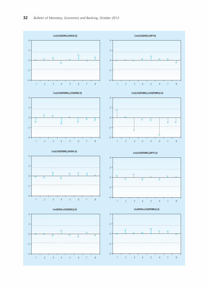
Correlogram
Autocorrelations with 2 Std.Err. Bounds
%��'$"('��))$*+$"('��))$*',�**
�!�
�!�
!
!�
!�
� � � � 9 � 7
%��'$"('��))$*+$"('-./�$*',�**
�!�
�!�
!
!�
!�
� � � � 9 � 7
32 Bulletin of Monetary, Economics and Banking, October 2012
%��'$"('��))$*+)�0�',�**
�!�
�!�
!
!�
!�
� � � � 9 � 7
%��'$"('��))$*+)123'�*
�!�
�!�
!
!�
!�
� � � � 9 � 7
%��'$"('-./�$*+$"('��)*',�**
�!�
�!�
!
!�
!�
� � � � 9 � 7
%��'$"('-./�$*+$"('-./�$*',�**
�!�
�!�
!
!�
!�
� � � � 9 � 7
%��'$"('-./�$*+)�0�',�**
�!�
�!�
!
!�
!�
� � � � 9 � 7
%��'$"('-./�$*+)123',�**
�!�
�!�
!
!�
!�
� � � � 9 � 7
%��')�0�+$"('��))$*',�**
�!�
�!�
!
!�
!�
� � � � 9 � 7
%��')�0�+$"('-./�$*',�**
�!�
�!�
!
!�
!�
� � � � 9 � 7

33Optimal Credit Growth
%��')�0�+)�0�',�**
�!�
�!�
!
!�
!�
� � � � 9 � 7
%��')�0�+)123',�**
�!�
�!�
!
!�
!�
� � � � 9 � 7
%��')123+$"('��))$*',�**
�!�
�!�
!
!�
!�
� � � � 9 � 7
%��')123+$"('-./�$*',�**
�!�
�!�
!
!�
!�
� � � � 9 � 7
%��')123+)�0�',�**
�!�
�!�
!
!�
!�
� � � � 9 � 7
%��')123+)123',�**
�!�
�!�
!
!�
!�
� � � � 9 � 7

34 Bulletin of Monetary, Economics and Banking, October 2012
Cointegration Test
�8����������� ������%���������������;�+�-�������&�&0��������� ���������G��������/������#���������������&�&0���������"�,������A���"��������+'333-��������
4�,��+��6� #�� 3/37
8������ ���'���������������*�#���$#�� &
�������&�%5.252 �1&�03252 �21�405'. �&�&&&'
@�������'�� �&�'%.0.' �.&�42&35 �%3�131&1 �&�&.14
@�������% �&�&30'20 �'.�53332 �'0�2321' �&�&3'0
@�������. �&�&&0.43 �&�1&%0%& �.�42'255 �&�2&'3
9�/��"�'($�& (������� ������� '���� ������� ����/::
�"F������������������ ������'���������������;�+�-�������&�&0��������� ���������G��������/������#���������������&�&0���������"�,������A���"��������+'333-��������
4�,��+��6� �!)(��� 3/37
8������ ���'���������������*�#���$ �!�����(�������&
�������&�%5.252 �.3�10.54 �%1�042.2 �&�&&&3
@�������' �&�'%.0.' �'1�'2'&% �%'�'.'5% �&�'502
@�������% �&�&30'20 �'%�3312% �'2�%525& �&�&140
@�������. �&�&&0.43 �&�1&%0%& �.�42'255 �&�2&'3
9�/��"�'($�& (������� ������� '���� ������� ����/::

35Global Financial Crises and Economic Growth : Evidence from East Asian Economies
GLOBAL FINANCIAL CRISES AND ECONOMICGROWTH : EVIDENCE FROM EAST
ASIAN ECONOMIES1
Arisyi F. Raz2, Tamarind P. K. Indra3, Dea K. Artikasih4, and Syalinda Citra5
As economies become more integrated in the midst of globalization, financial crisis that occurs in
one country can easily transmit to other countries, becoming global financial catastrophe in a short period
of time. In such event, strong economic fundamentals are particularly important to defend a country from
the contagious effect of the crisis. As evidence, due to the fragile economic fundamentals and lacking
government credibility, East Asian economies were easily attacked by the crisis in 1997 once the sentiment
deteriorated. Nevertheless, the region had learned its lessons in 1997 thereby proofing its resilience in
facing the global financial crisis that struck in 2008 by improving its economic fundamentals as well as
policymakers’ credibility. This paper starts with theories on economic growth and financial crisis. Further,
it empirically examines to what extent the financial crises in 1997 and 2008 affect East Asian economies
by using panel data econometrics. The evidence shows that, even though both crises have contributed
adverse impacts on East Asian economies, the magnitude of the 2008 crisis was relatively less severe than
that in 1997. Finally, this study also provides further discussions regarding how East Asian economies had
successfully minimized the impact of the global crisis in 2008.
Abstract
Keywords: Global Financial Crises; East Asian Economies; Economic Growth;Financial Market; Random
and Fixed Effects
JEL Classification: C330, E440, G010JEL Classification: C330, E440, G010JEL Classification: C330, E440, G010JEL Classification: C330, E440, G010JEL Classification: C330, E440, G010
1 Authors are extremely grateful for the helpful comments from Andi M.A. Parewangi. A previous version of this paper was presentedat the 6th Annual Workshop Bulletin of Monetary Economics and Banking, Jakarta, September 6, 2012.
2 Graduate of Institute for Development Policy and Management, University of Manchester.3 Graduate student at Graduate School of Business of Economics, University of Melbourne.4 Alumni of Department of Business and Asian Studies, Griffith University.5 Graduate student at Faculty of Economics and Business, University of Indonesia.

36 Bulletin of Monetary, Economics and Banking, October 2012
I. INTRODUCTION
Since the globalization era, the occurrence of financial crises has become more frequent
than before. One of the main reasons is the advancement in information technology, which, to
some extent, enlarges the magnitude of the crisis and acceleratesits spread to other regions or
countries. Another reason is the rapid development of financial sector.One of the examples is
the emergence of the so-called International Financial Integration (IFI). In this regard, Edison etal. (2002) explain that IFI refers to as “the degree to which an economy does not restrict cross-
border transactions” (page 1). Hence, due to the integrated financial systems, the occurrence
of localized financial nuisance in one country can result in a domino effect by perplexing other
integrated economies, leading to a global financial havoc.
In the last two decades, at least two major financial crises occurred, namely the 1997
East Asian Financial Crisis and the 2008 Global Financial Crisis. While the crisis in 1997 was dueto the lack of government transparency and credibility that led to structural and policy distortions
(see e.g. Corsetti et al., 1999), the economic turmoil in 2008 was mainly triggered by the rapid
innovation in financial products such as securitization practices and credit default swaps. It was
undermined further by property speculation and inaccurate credit ratings. In both cases, the
development of the crises spread to other regions and,in a short period,became global crises
due to the contagious effects amid globally integrated financial systems and rapid informationsharing.
Even though the sources of the crises may be varied, the consequences of financial crises
have always been associated with macroeconomic indicators, particularly economic growth.
For instance, during the East Asian crisis, East Asia plunged from being the fastest growing
region in the world to the region which several countries recorded negative income growth in
1998 such as Indonesia, Malaysia, Singapore, South Korea, Philippines and Thailand (AsianDevelopment Bank, 1999, Table A2). Later, Indonesia, Thailand and South Korea had to go to
the International Monetary Fund (IMF) for large bailout loan programs. On the other hand,
during the 2008 crisis, even though the source of crisis was due to the collapse of international
financial institutions in the west, especially those in the US and UK, some of East Asian countries
such as Malaysia, Singapore and Thailand were also dragged to the crisis by experiencing huge
financial encumbrance. Nevertheless, statistics shows that the impact of the crisis in 2008onEast Asian countries was not as deep as that in 1997. In addition,these countries managed to
recover rapidly. In this regard, many argue that East Asian countries have learned their lessons
in 1997 and endured the crisis in 2008 through fortified economic fundamentals.
Given these facts, it has become more important to conduct formal examination vis-à-visthe causes and consequences of financial crises, particularly in the context of East Asian region.
Hence, the objective of this paper is to measure the impact of each financial crisis on economic
growth in East Asian economies. Further, it is also important to analyze how East Asian economiesmanaged to minimize the impact of 2008 Global Financial Crisis. Until now,even though there

37Global Financial Crises and Economic Growth : Evidence from East Asian Economies
are already vast amount of literature analyzing the impact of the 1997 East Asian Financial
Crisis, most of these studies use the qualitative approach (for instrance, see Corsetti et al.,
1999; Lloyd and MacLaren, 2000; Jomo, 2001). In addition, due to its recent occurrence, the
study that examines the consequences of the 2008 Global Financial Crisis is also limited. Hence,
this paper aims to fill the gap in the literature by introducing a quantitative methodology and
comparing the consequences of both crises in East Asian economies. The rest of this paper isorganized as follows: Section 2 reviews the related theories on economic growth and financial
crises; Section 3 provides some methodology to measure the impact of both financial crises on
growth by using econometric modeling; Section 4 presents the empirical evidence and further
dicussions, and Section 6 concludes the paper.
II. THEORY
Growth Theories
Since the aim of this paper is to examine the impact of financial crises on economic
growth, firstly, it is necessary to derive the factors of growth from theoretical perspective. This
section, thus, introduces several growth theories that can be applied for the purpose of
methodology. According to the neoclassical view (e.g. Solow, 1956), growth is underpinned by
capital accumulation, which diminishes in the long run. As the consequence, a country willreach its “steady-state” in the long run, i.e. zero economic growth. One of the implications of
this growth model is that the less developed countries with open economies may eventually
catch up with developed countries as capital flows from the rich to poor countries that can offer
higher returns on investment, resulting in economic convergence (Todaro and Smith, 2006).
On the other hand, the so-called “new growth theories” contradict this theory by
suggesting that a country does not necessarily experience “steady-state” in the long run. Forinstance, a study by Lucas (1988) considers human capital as an endogenous variable of growth
and suggests that there are no diminishing returns to the combination of the accumulation of
human capital and capital goods, i.e. there is growth in the long run. These constant returnsto
scale are caused by the positive externality effects of knowledge, which affect the output of
individual firms in the economy. Another theory is proposed by Romer (1986, 1990), which
urges the importance of science and technology as the engine of economic growth. He arguesthat there are capital spillovers created by firms, which, in turn, create knowledge. Knowledge,
which triggers positive externalities, will prevent growth to diminish in the long run.
In application, human capital and knowledge spillovers can be obtained through FDI
and, to lesser extent, trade. In the scope of developing world, Yao and Wei (2007) argue that
FDI can act as a means to transfer these factors from developed countries to developing countries
since FDI accelerates the speed of General Purpose Technology6 (GPT) and introduces advanced
6 General Purpose Technologies are technologies that have impact on the whole national economy, such as computer and automobile.

38 Bulletin of Monetary, Economics and Banking, October 2012
technologies and know-how that do not exist in the developing countries. Developing countries,
thus, will utilise these factors as assets in order to enhance economic growth. Some literature,
however, suggest that FDI can distribute knowledge and know-how efficiently to a country
only if it meets several conditions. For instance, a hypothesis by Bhagwati (1994) points out
that trade policy plays a crucial role in determining the effectiveness of FDI in distributing
positive externalities in the country. In this regard, he argues that country with export orientationcan capture the spill over effects of FDI more efficiently and, thus, will have higher growth rate.
In short, this section shows that, based on the neoclassical growth theory, initial income
is an important factor of growth since countries with relatively lower initial income will grow
faster and catch up with those with higher initial income. Further, it also points out that capital
accumulation acts as the engine of growth in the short run. Meanwhile, new growth theories
argue that variables such as FDI and trade are also important in creating sustainable economic
growth in the long run by creating positive externalities through transfer of knowledge. Hence,for the purpose of methodology, these variables are considered as the main determinants of
growth. Before proceeding to the methodology, however, this paper will first investigate the
typology of financial crises in the following section.
Typology ofFinancial Crisis
The Reserve Bank of Australia (2012) defines a stable financial system as the one inwhich any activities of fund transfer from lenders to borrowers are being well accommodated
by financial intermediaries, market, and market structure. Financial instability, therefore, is a
condition where a collapse in financial system disrupts these activities and triggersa financial
crisis. Indeed systemic risks are always attached to any financial system, which according to
Davis (2001) is closely related to the wealth and soundness financial institutions. In other cases,
failure of market liquidity and breakdown of market infrastructure may also initiate the risks.
In his paper, Davis (2001) also outlines several theoretical framework that explain financial
instability, which include: 1)the debt and financial fragility theory, 2) disaster myopia theory,
and 3) bank runs theory.The debt and financial fragility theory argues that the economy follows
a cycle that consists of period of positive and negative growth (Fisher, 1933). With the upturn
of the economy, debt and risk taking activities increases. These create an asset bubble that will
lead to negative growth. Meanwhile, disaster myopia theory suggests that financial instabilitymay be caused bycompetitive behaviour of financial institutions that lead to a condition where
the credibility of borrowers were neglected and risks were undermined (Herring, 1999). On the
other hand, the bank runs theory explains the condition in which panic investors sell their
assets or drawdown their funds for fear that economic condition will be worsened (Diamond
and Dybvig, 1983; Davis, 1994). As the consequence, this will lead to a sudden plunge in asset
prices and liquidity crisis.
39Global Financial Crises and Economic Growth : Evidence from East Asian Economies
To their own extent, all of these three theories may explain the 1997 East Asian Financial
Crisis. Financial deregulations with inadequate regulatory supervision caused the asset bubble
that led to negative economic growth in East Asian economies. Meanwhile, the can rapid
expansion can also lead to credit crunch since credits were channelled recklessly to insolvent
borrowers in order to increase profitability. Last but not least, when investors realized that the
situation was already bad, they withdrew their funds, leading to massive capital outflows.
In addition to these basic theories, some literature suggest that financial instability canalso be caused by the role of international capital flows through international transmission,
such as trade patterns, exchange rate pressure and foreign investment, which causes the
“contagious effect” (see e.g. Chongvilaivan, 2010; Glock and Rose, 1998; Davis, 2001). For
instance, the Global Financial Crisis that occurred in 2008 was actually triggered by the Sub-
prime mortgage crisis originated in the US. Even though the crisis in the US can be explained by
the above theories, its spread to other regions, including East Asian region, was attributed tothe contagious effect of the Sub-prime mortgage crisis.
III. METHODOLOGY
This section provides research methodology in examining the impact of financial crises in
1998 and 2008 on East Asian economies. This paper collects data from World Bank’s WorldDevelopment Indicators (WDI) dataset for the period of 1990-2010. It obtains variousmacroeconomic variables of the selected East Asia economies, including the ASEAN-5 (Indonesia,
Malaysia, the Philippines, Singapore, and Thailand) and other notable East Asian economies,
i.e. China, Japan and South Korea.
In order to examine the relationship between economic growth and financial crisis, it is
necessary to develop the growth determinants first. By following the previous studies (for
instance, seeBarro, 2001; Chongvilaivan, 2010), growth is determined as a function of initialincome, capital expenditure, investment, and trade. Then, this benchmark growth model is
augmented with the crisis dummy. As the result, this paper defines the empirical framework as
follows:
(1)
where the subscripts i, i= 1, 2, …, N, and t, t = 1, 2, …, T, denote an economy i at the
time period t, respectively.
The dependent variable, Growth, is the GDP per capita growth rate. The firstexplanatory
variable, Income, is the logarithmic form of GDP per capita. Next, Capital is the gross fixedcapital formation as a percentage of GDP, which is included in order to capture the country-
specific productivity levels (Siegel and Griliches, 1992; Siegel, 1997). The rationale is that,
higher portion of capital accumulation leads to higher productivity level, thus increasing income
40 Bulletin of Monetary, Economics and Banking, October 2012
growth. FDI is the net foreign direct investment as a percentage of GDP. To some extent, the
role of FDI in contributing to growth is similar but not limited to that of capital. The reason is
because FDI also facilitates externalities and spillover effects, which enhance further the efficiency
of productivity of local firms (for instance, see Lim, 2001; Yao and Wei, 2007).Trade is a proxy
of international trade openness, which is measured by the ratio of exports and imports to GDP.
Chongvilaivan (2010) suggests that this variable represents the impacts of the global financialcrisis on an economy with respect to the commodity markets. Finally, a dummy variable, Crisis,is included in the model. It takes the value of unity during crisis period, i.e. the 1998 East Asian
Financial Crisis and 2008 Global Financial Crisis, and zero otherwise. For more details about the
variables, please refer to Appendix 1.
From this model, income is expected to have a negative sign. The rationale is based on
the neo-classical Solow Swan model, which suggests that economies with lower income level
will grow faster and catch up those with higher income level, resulting in income convergence(for instance, see Solow, 1956). On the other hand, capital and FDI are expected to have
positive relationships with growth.While the neo-classical Solow-Swan model suggests that all
type of capitals have similar role in contributing to economic growth, the “new growth theories”
suggests otherwise. As mentioned earlier, through FDI, these externalities can be transferred
from industrialised countries to the developing countries as important assets to enhance economic
growth further (for instance, see Yao and Wei, 2007). Due to this reason, this paper expectsthe coefficient of FDI to be bigger compared to that of capital since it has bigger role in
contributing economic growth.
The relationship between trade openness and income growth is more complex, depending
on whether international trade causes trade creation or trade diversion. The former occurs
when international trade increases the welfare of the members of trade alliance without
sacrificing that of the non-members. On the other hand, the latter occurs when trade allianceis formed at the expense of its non-members and thus welfare-decreasing. In this regard, the
relationship between trade openness and income growth depends on which of these influences
has stronger effect.
Lastly, the coefficient of crisis dummy is expected to be negative, which is intuitive.
Nevertheless, the coefficient of 1998 East Asian Financial Crisis is expected to be bigger than
that of 2008 Global Financial Crisis since, as mentioned earlier, East Asian countries had strongerfundamentals and better resistance during the 2008 Global Financial Crisis.
Due to the panel nature of the data, this paper uses the fixed effects and random effects
methods for the estimation purpose. By using fixed effects, the model controls for unobserved
heterogeneity by assuming that each country has its own effects that may influence the
dependent variable. In this model, each country’s heterogeneity is captured by the intercept
and associated with the independent variables. Thus, the nature of fixed effects prevents the
estimation to suffer heterogeneous bias and thus the model always gives consistent results.The
41Global Financial Crises and Economic Growth : Evidence from East Asian Economies
presence of fixed effects can be tested by conducting an F-test. The fixed effects are jointly
significant when the null is significantly rejected. Another model is the random effects model,
which assumes that the variation across countries is random and uncorrelated with the
independent variables. Different from the fixed effects model, the presence of random effects
can be tested by using a Breusch-Pagan Lagrange Multiplier test.
IV. RESULT AND ANALYSIS
This section provides the estimation results of Equation (1). Nevertheless, before proceeding
to the results, it is necessary to justify the stationarity of the variables included in the model. As
shown earlier, this study utilizes data set that covers a long period, i.e. 21 years. Thus some
variables may contain a unit root. If unit root is present, these variables become non-stationary
and cause the traditional estimation methods cannot be used since they can result in a spurious
regression. In this case, a test for cointegration is necessary for the non-stationary variables.
There are several panel unit root tests that can be performed such as Hadri (2000), Levin,
Lin and Chu (2002) and Im, Pesaran and Shin (2003). In this regard, this paper employs the
Levin, Lin and Chu (2002) to test the presence of unit root in the variables. The results confirm
the stationarity of these variables since the null of a unit root is significantly rejected at the 5%
level for all variables (Appendix 4). Therefore it is not necessary to do the cointegration test.
Consequentially, Equation (1) can be estimated by using the fixed effects and random effectsmodel.
In addition, due to the nature of the data, serial correlation and/or heteroscedasticity
may present, which can lead to inconsistent and biased estimation results. Hence, this paper
corrects these problems by treating each country effects as a cluster in order to estimate the
correct standard errors with the Huber/White cluster-robust covariance estimator in all regressions.
Benchmark Growth Regression
The first column of Table 1shows the results of the fixed effects estimation, whereas the
second column shows the results of random effects estimation. Overall, the results are consistent
with economic theory and expectations. The first explanatory variable, income, is not significant
in the first column but significant at 1% in the second column with negative coefficient.
Next, capital is significant in both columns, even though the magnitude is bigger in the
random effects. Overall, despite the relatively higher magnitude, this result is consistent withthe previous studies (for instance, see Chongvilaivan, 2010). Hence, it proves that higher capital
accumulation results in higher productivity and enhances income growth.Further, FDI is also
significant at 1% and positively correlated with income growth in both regressions. In the fixed
effects model, according to expectation, the magnitude of FDI is bigger than capital, which is

42 Bulletin of Monetary, Economics and Banking, October 2012
also consistent with the previous studies (for instance, see Stopford et al.,1991; Azman-Saini
and Ahmad, 2010). However, contradicting the result in the fixed effects model, the random
effects model shows that the coefficient of capital is slightly higher than that of FDI.
Lastly, trade has a negative sign and is only significant in the random effects. The weak
evidence of the relationship between trade openness and income growth may be attributed to
the presence of trade creation and trade diversion (Viner, 1950).If the effect of trade diversion
in the region is bigger than trade creation, trade openness will not result in output growth.
The F-test of the fixed effects strongly rejects the null, justifying the presence of a correlation
between the explanatory variables and heterogeneous effects in errors. In other words, the
fixed effects estimation provides unbiased and consistent estimators. On the other hand, theBreusch-Pagan Lagrange Multiplier test for random effects is not significant at 10% level,
failing to reject the null of individual effects are equal, i.e. there are no random effects. As the
consequence, the random effects estimation is biased and inconsistent.
Economic Growth and Financial Crises
Next, the discussion of this paper moves to the impact of financial crises on economic
growth in East Asian economies. As shown in the methodology, this paper employs crisis
���������� ���������� �����������
��������
��������
����������� ��������������� ����������� � ��� �� ���� ���������� ���������������� ������� �� � �� ������ ��� � ��
���� ������ ������ ������
����� �!"�#$%&
���%�"!%���$&
'���( )��#$!%����&
*���� ��%�"��!���"$&
+,' ���� ���!�����&
-��� ����$�!���"#&
��� �� ���"�
���% ����!���� &
��)�����!�����&
��%�%���!�����&
�����#��!���)%&
.*� �� ��%%
��/����� ��%�
��� �/ � ����
���� ���� ����0�������� �"$�"$0����������� $$

43Global Financial Crises and Economic Growth : Evidence from East Asian Economies
dummy in order to measure the impacts of financial crises on East Asian economies. The first
crisis dummy is for the 1997 East Asian Financial Crisis. In this regard, even though the crisis
struck in 1997, the dummy variable takes the value of unity in 1997-1998 by considering the
lagging effect of the crisis. The second one is for the 2008 Global Financial Crisis. Similarly,
since the lagging effect also exists, the crisis dummy is assigned in the year when the crisis
struck and the following year, i.e.2008-2009.
Table 2 presents the benchmark growth model that is augmented by the crisis dummies.In the first two columns, it is augmented with the 1997 East Asian Financial crisis. In general,
the relationship between growth determinants and income growth is consistent with the initial
benchmark regression.Next, as expected, the crisis dummy is significant in both models with
relatively similar magnitude. According to the estimation, under ceteris paribus, the presence
of East Asian Financial crisis causes East Asian economies to experience negative income growth
of around 6%.
��������������������� ���������������������
��������
��������
����������� ��������������� ����������� � ��� �� ���� ���������� ���������������� ������� �� � �� ������ ��� � ��
���� ������ ������ ������
� �# �!"�$�"&
'���( ��"%�!��#� &
������� ��%#����!�����&
+,' ���%$���!���"�&
-��� ����$!����#&
��� �� %�#��#
.*� ��
��/����� ���
��� �/ � ����
���� ���� ���%
0�������� �"$
0����������� $
���� ������ ������ ������
����)�!��#%�&
�%��# ���!���)��&
���� �!%����&
���)�#���!���%%&
"��#��!)�% �&
���%%)���!�����&
��)�����!���) &
���$��!���$�&
��)� ���!�����&
��%�����!����%&
��)%$��!�����&
��� ����!�����&
�����!���� &
�����#!��� #&
�����!���%$&
1��������� ���#�����!��)$�&
���#$$���!��)��&
� �
2����������� � � �)������!��#��&
�%��%$��!��$ #&
$#��$
���� ��%�
��%#"
����"
���%�
�"$ �"$ �"$
$ $ $

44 Bulletin of Monetary, Economics and Banking, October 2012
Once again, this paper tests which of these estimation methods provides better estimation
by looking at the F-test (for fixed effects) and LM test (for random effects). Similar to the
benchmark regression output, F-test significantly rejects the null at 1% level, whereas LM test
fails to reject the null at 10% level. Thus, in the East Asian Financial Crisis, fixed effects estimation
is the better model since it provides consistent and unbiased estimators.
The last two columns exhibit the benchmark growth model with 2008 Global Financial
crisis. Surprisingly, the fixed effects model shows that the magnitude of income becomeshigher if the model is controlled for 2008 crisis, implying that countries with higher income
tend to grow faster even though the evidence is very weak (i.e. only significant at 10% level of
confidence). One possible explanation is because countries with relatively higher income,
particularly Singapore, managed to attain income growth beyond 10% after the crisis even
though it recorded negative growth when the crisis struck, whereas countries with relatively
lower income such as Indonesia only achieved stable growth despite the fact that it successfullyavoided negative growth when the crisis struck.
On the other hand, other variables, i.e. capital, FDI and trade, do not differ significantly
from the previous estimations. Finally, the Global Financial Crisis dummy is significant at 5% in
both regressions even though the impact of the crisis is higher in the fixed effects model.
Furthermore, the result is also consistent with the expectation of this paper, i.e. the 2008
Global Financial Crisis has smaller adverse impact on income growth in East Asian economies.
Further Discussion and Analysis
Other than the coefficients for income and trade, estimation results of the model are
inline with expectations and consistent with previous studies. The objective of this section,
thus, is to provide further discussion and analysis on the estimation results. First, the coefficients
for income in the benchmark model as well as the models augmented by the 1997 East AsianCrisis dummy show insignificant results with signs that are not inline with expectations. However,
the estimation result from the model augmented by the 2008 Global Financial Crisis dummy is
significant at 10% level of significance and similar with previous case it is not of expected sign.
These results indicate that the growth model used in this paper only weakly support Solow’s
(1956) neo-classical growth theory, particularly that that is relating to economic convergence.
Second, all of the estimated coefficients for capital are significant and positive which is
as expected. This shows that capital accumulation is indeed leading to economic growth.However, estimation results for FDI, which are more significant than those for capital, indicate
the presence of knowledge transfer from the more developed economies to the less developed
one through FDI. These results support the studies conducted by Lim (2001) and Yao and Wei
(2007), which suggest that FDI facilitates externalities and spillover effects that will enhance
efficiency of productivity of local firms. In turn, these will support economic growth.

45Global Financial Crises and Economic Growth : Evidence from East Asian Economies
Third, all of the estimated coefficients for trade are insignificant and of conflicting signs,
which suggest that the model provides insufficient evidence for us to make any inference
about the correlation between trade openness and income growth. Nevertheless, these results
indicate that the data used in this paper support the study of Chongvilaivan (2010), whose
paper proposes the insignificance of trade variable as the result from the presence of trade
creation or trade diversion. Therefore, the effect of trade on income growth depends on whetherthe welfare of trade alliance’s members is increasing at the expense of non-members or not.
Lastly, even though both of the estimation results for crisis dummies show negative sign,
the 1997 East Asian Crisis dummy shows higher magnitude compared to the 2008 Global
Financial Crisis dummy. This is in accordance with expectation since the 1997 East Asian Crisis
was happening in the East Asian region and was a result from causes internal to the region,
including: 1) lack of policy credibility and 2) inadequate financial infrastructure that accompanied
financial deregulations.For the former, as argued by Raisah (2001), this crisis was initially triggeredby abusive state intervention and less effective industrial policies in the region. As for the latter,
financial deregulations inadequate financial infrastructure and poor banking supervision
encouraged risky investments without sufficient risk assessment led the credit bubble and
collapse of the financial sector (for instance, see Radelet and Sachs, 2000). These weak economic
fundamentals reflect the “financial fragility” as the main issue of East Asian economies, which
triggered the crisis in 1997 and hit the region’s economy severely (see Appendix 5 for statisticson macroeconomic variables during both financial crises). Further, this crisis was deepened due
to its spread to the real sector, which hurt the borrower’s business and, massive capital outflow.
On the other hand, the crisis in 2008 had smaller impacts on the region’s economy since
the region only suffered the “contagious effect” of the crisis that was actually originated in the
developed economies. To some extent, this result supportspaper, which suggests that the
divergence may relate to the externality of the 2008 Global Financial crisis (Chongvilaivan,2010; Emmers and Ravenhill, 2011). Nevertheless, indeed the improvements in the fundamentals
of East Asian economies prior to 2008 Global Financial Crisis werealso much attributed to the
multidimensional reforms that followed 1997 East Asian Financial Crisis.To be more
specific,Goldstein and Xie (2009) point out that large holdings of foreign reserves, improved
financial structure, high share of regional trade, and stances toward countercyclical monetary
and fiscal policies would assist the region to weather negative impacts from the crisis.
V. CONLUSIONS
World’s financial system, reinforced by development in information technology, has
strengthened financial integration between countries around the world. Despite the advantages
of this advancement, however, financial integration has also caused financial crises to spread
more easily and rapidly, undermining connected economies. Due to this reason,studies aboutfinancial crises have become more important than ever since. In this regard, the objective of

46 Bulletin of Monetary, Economics and Banking, October 2012
this study is to better understandthe causes and consequences of the recent financial crises by
providing comprehensive analysis in order to prevent the occurrence, or at least minimize the
impact,of financial crisis in the future.
This study has revealed important findings about the main impacts of financial crises on
East Asian economies. First, this study has investigated the impact of both 1997 East Asian
Financial Crisis and 2008 Global Financial Crisis by using a quantitative approach, i.e. panel
regression. The result shows that even though both crises had adverse effects on the economyof the region, East Asian economies had become more resilient during the crisis in 2008 compared
to that in 1997. Further, this paper finds out that minimized impact of the crisis in 2008
occurred since, in addition to the “externality” of the crisis, most East Asian economies had
learned its lesson after the 1997 East Asian Financial Crisis by strengthening economic
fundamentals, underpinned further better government credibility and accountability.
Concerted efforts to restructure the banking and financial sectorby East Asian governmentsthat follows the 1997 East Asian Financial Crisis had increased resilience to economic crises.
Included in the reforms was better supervision on this sector as opposed to period prior
deregulations and suspensions as well as merging troubled financial institutions. Capital was
also injected to assist with liquidity problem. Apart from banking and financial sector reform,
higher requirement for corporate transparency was also demanded to increase credibility of
the private sectors. Altogether, these reforms had strengthened economic fundamentals ofEast Asian countries. Another most important things that had better preparedEast Asian countries
in facing the 2008 Global Financial Crisis was improvement in foreign exchange reserves
condition, which aiding governments in defending the economy during the crisis.
Despite its findings, the scope of this study is limited to country-level data and analysis.
Hence, further studies should focus more on the industry-level analysis and thus have to be
facilitated by the availability of industry-level data in order examine the sensitivity of eachindustry in anticipating the financial crises.In addition, the estimation results in this study can
be improved by adding interaction variables between crisis dummy and other independent
variables as well as introducing the GMM estimation in estimating the model in order to capture
the simultaneous equations in the model.

47Global Financial Crises and Economic Growth : Evidence from East Asian Economies
REFERENCES
Asian Development Bank (ADB). (1999). Asian Development Outlook 1999, Manila: Asian
Development Bank.
Azman-Saini, W.N.W., Law, S.H., & Ahmad, A.H. (2010). FDI and economic growth: New evidence
on the role of financial markets, Economic Letters, Vol. 107, pp. 211-213.
Barro, R.J. (2001). Economic growth in East Asia before and after the Financial Crisis, National
Bureau of Economic Research Working Paper Series, No. 8330.
Bhagwati, J. (1994). Free trade: Old and new challenges, Economic Journal, Vol. 104, pp. 231-246.
Chongvilaivan, A. (2010). Global Financial Crisis and growth prospects in Asia-Pacific: A sectoral
analysis, paper presented at The 26th Conference of the American Committee for Asian
Economic Studies, Kyoto, Japan, 5-6 March.
Corsetti, G., Pesenti, P., &Roubini, N. (1999). What caused the Asian currency and financial
crisis? Japan and the World Economy, Vol. 11, pp. 305-373.
Davis, E.P. (1994). Market liquidity risk,Kluwer Academic Publishers.
Davis, E.P. (2001). A typology of financial instability, Oesterreichsche National Bank Financial
Stability Report 2, pp. 92-110.
Diamond, D., Dybvig, P. (1983). Bank runs, deposit insurance and liquidity, Journal of Political
Economy, Vol. 91, pp. 401-419.
Edison, H.J., Levine. R., Ricci, L., &Sløk, T. (2002).International financial integration and economic
growth, National Bureau of Economic Research Working Paper Series, No. 9164.
Emmers, R., Ravenhill, J. (2011), The Asian and global financial crises: consequences for East
Asian regionalism, Contemporary Politics, Vol.17 no. 2, pp. 133-149
Fisher, I. (1933). The debt deflation theory of great depressions, Econometrica, Vol.1, pp. 337-
357.
Goldstein, M., &Xie, D. (2009). US credit crisis and spillovers to Asia, Asian Economic Policy
Review, vol. 4, pp. 204-222.

48 Bulletin of Monetary, Economics and Banking, October 2012
Hadri, K.(2000). Testing for stationarity in heterogeneous panel data, The Econometrics Journal,
Vol. 3, no. 2, pp. 148-161.
Herring, J. (1999). Credit risk and financial instability, Oxford Review of Economic Policy, vol. 15,
No. 3, pp. 63-67.
Im, K.S., Pesaran, M. H. & Shin, Y. (2003). Testing for unit roots in heterogeneous panels, Journal
of Econometrics, Vol. 115, pp. 53-74.
Jomo, K.S. (2001). Growth after the Asian Crisis: What remains of the East Asian Model?, G-24
Discussion Paper Series, No. 10.
Kawai, M., Newfarmer, R., & Schmukler, S. L. (2003). Financial crises: Nine Lessons from Asia,
Japan Ministry of Finance PRI Discussion Paper, No. 2003-5.
Khor, M. (1998). The economic crisis in East Asia: Causes, effects, lessons, Third World Network.
Kindleberger, C. P. (1978). Manias, panics and crashes, A history of financial crises. Basic Books,
New York.
Levin, A., Lin, C.F. & Chu, C. (2002). Unit roots tests in panel data: Asymptotic and finite sample
properties, Journal of Econometrics, Vol. 108, pp. 1-24.
Lim, E.G. (2001).Determinants of, and the relation between, foreign direct investment and growth:A summary of the recent literature, IMF Working Paper, WP/01/175.
Lloyd, P.J., & MacLaren, D. (2000). Openness and growth in East Asia after the Asian crisis,
Journal of Asian Economics, Vol. 11, pp. 89-105.
Lucas, R.E. (1988). On the mechanism of economic development, Journal of Monetary Economics,
vol.22, pp. 3-42.
Rasiah, R. (2001). Pre-crisis economic weaknesses and vulnerabilities. In: Jomo KS, ed. Malaysian
Eclipse: Economic Crisis and Recovery, London: Zed Books, pp. 47–66.
Radelet, S. and Sachs, J. (2000).The onset of East Asian financial crisis, National Bureau ofEconomic Research, pp. 105-162.
Research Bank of Australia. (2012). About financial stability. Retrieved from http://
www.rba.gov.au/fin-stability/about.html on 7 December 2012.
Romer, P.M. (1986). Increasing return and long run growth, Journal of Political Economy, vol.
95, pp. 1002-1037.
_______. (1990). Endogenous technological change, Journal of Political Economy, vol 98, no. 5,
pt. 2.
Siegel, D. (1997). The impact of computers on manufacturing productivity growth: A multiple-indicators, multiple-causes approach, Review of Economics and Statistics, vol. 79, pp. 68-78.

49Global Financial Crises and Economic Growth : Evidence from East Asian Economies
Siegel, D. & Griliches, Z. (1992). Purchased services, outsourcing, computers, and productivity in
manufacturing, National Bureau of Economic Research Working Paper Series, No. 3678.
Solow, R.M. (1956).A contribution to the theory of economic growth, Quarterly Journal of
Economics, LXX, pp. 65-94.
Stopford, J., Strange, S., &Henley, J. (1991). Rival States, Rival Firms: Competition for World
Market Shares, Cambridge: Cambridge University Press.
Todaro, M. P, & Smith, S. C. (2006). Economic Development, Addison Wesley, Boston.
Viner, J. (1950). The Custom Union Issue, New York: Carnegie Endowment for InternationalPeace.
World Bank. (various issues). World Bank Indicator (http://data.worldbank.org/indicator/)
Yao, S. & Wei, K. (2007). Economic growth in the presence of FDI: The perspective of newly
industrialising economies, Journal of Comparative Economics, Vol. 35, pp. 211-234.

50 Bulletin of Monetary, Economics and Banking, October 2012
APPENDICES
������� ��!��������"�����������
��������
����
����������
1������ �� ���� ���/����� ��2,3� ���������� �������������������� ����2,3� ����������������( ���������������� ���(��� �������������2,3��������� �4����� ����� ��(����������� ��� ������� ��� �������� ������ ����(�����������������5 ����(�������������� ���������� ����� ���� ���� ���������'����������� �/������(�6���� ������������ �� ����������������� ���� �������� �� �������� ������������������� ����� ��!75�� �� ����&
�� ��� 2,3� ����������������( ���������������� ���(��� �������������2,3���� ��(����������� ��� ������� ��� �������� ������ ����(�����������������5 ����(�������������� ���������� ����� ���� ���� ���������'����������� �/������(�6���� ������������ �� ����������������� ���� �������� �� �������� ������������������� ����� ��!75�� �� �����������8�9��������&
������ 2��������������(�����!���( ����������( ������� ��( ��&�������������������������������� ��5 ���� ������ ����(������ ������ ����� � � ������ ����� ��+�5 ���� �������� ���� �(���� ( ���!� �� ������ ��������������&:�����(����� ����� ;���( ��������� �:����� �����������������������/�������� ��6 ��������������������� ���������������� � ��� ������/ �����������(( ����������������������������'�� ����� ��� ����6��������� �������(���( �� (���������� 5� �� ������������������������������ ����</��6������� ���<1������������ �##)901� ���;����������� ������� � �� ���� ������ � � ������� ���(������ !75�� �� � �� � �� 2,3&
��� +�� ������ ����� ��( ���� �� � ������/������ ��( ������;��� ��������(���� ( ����� � ��!��� �� ����(�� ������������6&���� �� ����� �� ���������� ����(���� ������������� ��� �����'����� ��(�� ;������������ ��� ��( ���� ���������� ������� �(����������������� �(������������/����� ������ �����( ����!75�� �� ������2,3&
�������������� -� �� ������� 5���������(�������2,3!75�� �� ������2,3&
������ 1��((�������� ��� �� � ���� ������ �� ��������!/� �� ��## 7���1����+����������������%��$2�����+��������������&�'���6 ��� ���� ��������������� �������������������� ����������� ����&�
������� ��#$����%�#����������&'�����(��))*+�*�*,
��������
���� )� %�$�) )��" ���%$ �)�"���� ��� )� )�$"� ��"�� %��$" ��"�������� )� %��$ � ��"� ���)" �$�%�)��� )� %�#�� )�" % ����% %%���$�������������� )� %��$) ���� ���)) )%�%""
��� ���� ���� ��� ���

51Global Financial Crises and Economic Growth : Evidence from East Asian Economies
������� �-������������.���� ��/�0�����������!��������
�� ��� ����������� ���"" �������� ��)#� ���� ������������������� ���)% ���)� ���%$ �����
������ ��� ��� ������������
������� �12�3���2���� $������/���������$��������
���� $�$ � ��$"# ������� ��� �#�� %� � ����)������ ���) %���" ���� ��� ���)"% ��%#% ������������������� ��$" %�%#� �����
�������� ����� ������� ������

52 Bulletin of Monetary, Economics and Banking, October 2012
APPENDIX 5. OTHER MACROECONOMIC STATISTICS
Appendix 5.1.GDP percapita in East Asian economies (annual growth rate, %)
Appendix 5.2.Foreign exchange reserves of several East Asian countries (in million)
���� ���� ���� ���� ���� ���� ���� ���� ���� ���� ����
����� ������ �� ����� ��������
������������������������ ������������
�� ������� ������������ ��� �!����"����������
#$%&&'
#&%&&'
$%&&'
&%&&'
($%&&'
(#&%&&'
(#$%&&'
���� ���� ���� ���� ���� ���� ���� ���� ���� ����
��������� �� ��)�*��% ��������
����������� ������� � ��������
�� ������� ������������ ��� �!����"���������� �����+��,��� �!����"���-������%
.&&%&&&
/$&%&&&
/&&%&&&
#$&%&&&
#&&%&&&
$&%&&&
&

53Global Financial Crises and Economic Growth : Evidence from East Asian Economies
������� �4-0�/������������������������������5��))6+�))7
� ! � "
����� %�$ ���$'���� ��� "�% �$��=���� ��$ � � *������� %� � �)3�������� � ��" # �)9������� % ���)9����>�� � ��� ��-������� ��" $ ��
#��������
9���� ?@����A��64�@����, � ���( ��'��������
'���� ��� ��% ��� ��) �%�" �)��
*������� ���� �� %�� ���$ �)�%
B ����>�� � ��% ��� ���� ���% �%�#
-������� )�% %�� ���# �)�� �)
'���� ��� � )�# ��� �� ��� ��$
*������� )�" ��� � )�# %$�% ��)
B ����>�� � )�� ��� ��� ��% ����� )�%
-������� %�# ��" ��% �%�# ����� ����
������� �41������������$�(�.�����������������������5��))*+�)))
� $ � % � ! � " � � $� & � % � ! � " �
'���� ��� ���� ��� ��" ��� "�) )� %"�% %"�� %"�� %)�
*������� " %�� %�� )�% ) )"�" ) �� ) �) )#�" )$
B ����>�� � %�� ) %�" "�$ "�) )��" ))� ))�) ))�$ ))��
-������� ��# ��� ��# )�� ��� )��� )) )%�� )��# )�
���� ���������� ����������
9���� ? B�� � ����9����!�##$?���� ��&:1,A!�###&:A��6��-�������A��6'���� ���A��6��>�� �A��60 ����*�������;��� ����(=�(�!%���&�
� $� & � % � ! � " � � $� & � % � ! � " �
�������������� ������� ����������!����
'���� ��� )��) %#�" %$� %%�� �#�) ���) �)�� �%�) � ���
*������� ) �� �%�� �)�� %"�$ %%�) ���# ���� ���$ �%�$ ���
B ����>�� � )"�$ )"�$ )��� %#�$ %$ ���% �)�� ���$ ��� ���
-������� �� ���� ))�) %%�% %� ���" �$�� ���# �%�$ ��
� "!�" � $� ' � (� & � ! � " �
��������� ���� �"�"��������
� $� & � % � ! � " �
���� �# �������

54 Bulletin of Monetary, Economics and Banking, October 2012
This page is intentionally left blank

55The Dynamics Spillover of Trade between Indonesia and Its Counterparts in Termsof AFTA 2015 : A Modified Gravity Equation Approach
THE DYNAMICS SPILLOVER OF TRADE BETWEENINDONESIA AND ITS COUNTERPARTS IN TERMS
OF AFTA 2015 : A MODIFIED GRAVITYEQUATION APPROACH
Barli Suryanta1
The forthcoming 2015, ASEAN is being confident to implement ASEAN Free Trade (AFTA). The
existence of AFTA is to outstrip trade liberalization due to augment trade volume significantly and transaction
easing as well among the members of AFTA, mainly by inducing lower tariffs some certain commodities
up to 0%. This paper is conducted in order to examine on what prominent commodity of Indonesia
compared to its counterparts namely Brunei, Malaysia, Philippines, Singapore and Thailand. These Indonesia
counterparts are selected therefore they were the founding of ASEAN. Furthermore, this paper utilizes a
modified Gravity Equation model. This robust model has an effort to estimate the significance of some
parameters of variable from model equation. Thus, it can be detected that what are from these variables
from a model equation being as a key determination factor to influence trading transactions. This paper
also assesses the adjusted R-squared due to which Indonesia counterparts incur some vantage points as
well as beneficial for Indonesia in terms of AFTA. The novelty contribution of this paper is to reveal the
dynamics trade spillover between Indonesia some strategic sectors and its counterparts. By doing so,
Indonesia is expected to be a dominant player in AFTA 2015 and taking some advantageous from AFTA
into Indonesia account.
Abstract
Keywords: AFTA 2015, a modified gravity equation model, analysis of data panel
JEL Classification: C33, C51, F15JEL Classification: C33, C51, F15JEL Classification: C33, C51, F15JEL Classification: C33, C51, F15JEL Classification: C33, C51, F15
1 Corresponding author : A Junior Lecturer and a Researcher at the School of Business and Management, InstitutTeknologi Bandung(SBM ITB), Indonesia; tel. +62-22-2531923; email: [email protected].

56 Bulletin of Monetary, Economics and Banking, October 2012
I. INTRODUCTION
In the autarky situation, Indonesia has free to choose the beneficial partners for trade
outside ASEAN. Nonetheless, since 1992 until today, the condition had been significantly altered
by the existence of AFTA. The founding members, namely Indonesia, Thailand, Malaysia,
Singapore, and Philippines and also plus Brunei were being the first group to utilize Common
Effective Preferential Tariff (CEPT) Scheme. The CEPT by the terminology is a cooperativearrangement among ASEAN Member States that will reduce intra-regional tariffs and remove
non-tariff barriers over a 10-year period commencing January 1, 1993 (asean.org). Then, the
second group which has composed of Cambodia, Lao, Myanmar, and Vietnam would allow to
possess the same CEPT as the first group under different circumstances and it might be initially
after the first group is inferred establishing to some extent.
Moreover, while the strategy of the CEPT is still on the track, in as much, ASEAN alreadyhas built two new commitments to foster the economic integration in ASEAN through ASEAN
Economics Community (AEC) Blueprint 2008 and AEC chart-book 2009. In this both scheme,
the essence is the priority sector to be fully integrated in year 2015. Regarding these accords,
ASEAN featured seven sectorswhich are compatible with ASEAN competitive advantage in the
foreseeable future. The seven sectors are agro-based products, automotive, electronics, fisheries,
rubber-based products, textiles and apparels, wood-based products. Nevertheless, this paperwould be determining the selected sectors such agro-based sector, fisheries, rubber based-
products, and wood based products. These sectors are chosen because actually, Indonesia
possesses more competitive advantage of these rather than its competitor.
Linkage to this context, this paper has a purpose to assess these selected sectors. Most
importantly, the novelty of this paper is to define whether the strength sector or the weakness
sector, even the poor sector comparing Indonesia to its selected ASEAN trading partners,namely Malaysia, Philippines, Singapore, Thailand and Brunei in accordance with AFTA 2015.
Furthermore, to develop the rigorous analysis, this paper employs a modified Gravity Equation
model. This model has a function to describethe robustness of the interpretation from theresulted
regression due to the significant coefficients of the variable and the adjusted R-squareas well.
Thus, this study can spill the dynamics terms of trade between Indonesia and others in proper
way.
The next session of this paper outline the theory of economic integration, session twodiscuss the methodology and the data used, while the estimation result of the gravity model
and its analysis is presented in session 4. Conclusion and implication of this study is presented
on the last session, and will close the presentation of this paper.

57The Dynamics Spillover of Trade between Indonesia and Its Counterparts in Termsof AFTA 2015 : A Modified Gravity Equation Approach
II. THEORY
The Economic Integration
Venables (2000) said that economic integration called as a regional economic integration
which occurs when countries come together to form free trade areas or customs unions,
offering members preferential trade access to each other’ market. He emphasizes regionalintegration into ‘deeper integration in terms of international trade’ that it can be pursued by
going beyond abolition of import tariffs and quotas, to further measures to remove market
segmentation and promote integration. Economic integration is defined as the elimination of
economic frontiers between two or more economies (Pelksman, 2006). He said that the
fundamental significance of economic integration is the increase of actual or potentialcompetition. Furthermore, competition by market participants is likely to lead to lower pricesfor similar goods and services, to greater quality variation and wider choice for the integrating
area, as well as to a general impetus for change. Product designs, services methods, production
and distribution systems and any other aspects become subject to actual and potential challenge.
They may induce changes in the direction and intensity of innovation and in working habits.
Proposed by El-Agraa (1997), there are different forms of integration but the essence of
the integration arrangement is the discriminatory removal of all trade obstacles between at
least two participating nations and the promotion of some form of cooperation and coordinationbetween the participating countries. The table 1 below exhibits the stages regarding El-Agraa:
�������������� �����������������������������������������
����
������ ��
��������������� ��� �������
�����������
���������
�� ������ ������
����������� ����������
�����������������
��������� � ��
������ ��� ��������� ���� � ��
������� ��� ��������� ���� � ��
��������� !"���#$%&&'(
FFFFFurthermore,in free trade areas the member countries remove all trade impedimentsamong themselves but each country retains the right to determine their policies in relation to
non-participating countries. The agreement usually includes the elimination of tariffs and
quantitative restrictions on trade. The rules of origin are the basis of the agreement. The rules

58 Bulletin of Monetary, Economics and Banking, October 2012
of origin imply that only those commodities that originate from a member state are granted
from tariff. The examples of free trade areas include the European Free Trade Association
(EFTA), comprising of the UK, Austria, Denmark, Norway, Portugal, Sweden, Switzerland and
Finland and the North American Free Trade Area (NAFTA) formed in 1993 by the United
States, Canada and Mexico. Then, in customs unions, member countries, as in free trade
areas, remove all trade impediments among the participating countries.
Thus, the member countries harmonize their trade policies and, in particular, have commonexternal tariffs on imports from non-participating countries. The most well known customs
union is the European Common Market formed in 1957 by West Germany, France, Italy,
Belgium, the Netherlands and Luxembourg. The item of common markets are customs unions
with the added feature that there is free mobility of factors of production i.e. labor, capital,
enterprises and technology, across the participating countries.
In 1992 the European Union (EU) achieved the status of a common market.Economicunions are common markets where there is unification of monetary and fiscal polices. Monetary
policy is managed by a central bank. The union will have a single currency, in the case of the
European Union, the euro. There is a central authority to exercise control over these matters.
This is considered to be the most advanced form of economic integration. Finally, the total
political union can be defined as the participating countries become one nation. The central
economic authority is supplemented by a common parliament and other institutions. As thehighest stage, the total political union had been already implemented by European Union.
In addition, Balassa (1961) introduced theprominent crucial stages to aim the economic
integration. These stages can be expressed as table 2 below:
������������������ �����������������������������������
� ���
� �����
���������!���$��!(
�������!���������)������#%&*%
����� ��� ��
��� �������������� �+���� �������������������� !�������������� ���� ������� �$���������(�"� ����+ �������� ��
� ����!
��������� ��$�,(
�������� �"� ��� � ��� �� ���,������� �����������-��� ����� ��� ������ �$�����#��������#������( ������. �+���
�������
� ����"
������/��-��$�/(
!�,.+ �+�������� �+������� �� �������������������
� ����#
������ �,� ��
!�/. �+������"����+����� ��� ������ ���������� ���� � �� ��������������� ��� � ��� �������� ���� � �� ��+������ � ��
� ����$
����������� �0���"��� ��
,� ��� �����������# ����#��� ���������������� ������ � �� ���� �"������������ �������+�� ��.+������ � ������� �� �"
���+�������������

59The Dynamics Spillover of Trade between Indonesia and Its Counterparts in Termsof AFTA 2015 : A Modified Gravity Equation Approach
The crucial stages are presented sequentially for analytical reasons. However, there is no
mandatory to follow the Balassa’s crucial stages. The European Economic Community (EEC)
launched a customs union (CU), not free trade areas (FTAs). In contrast NAFTA started with
strategy of free trade areas (FTAs). Balassa’s crucial stages of economic integration provide the
systematic of concept in order to attain the real economic integration.
Fundamental Theory of Trade Integration
International trade in goods and services takes place because countries have different
resource endowments and labor skills and because consumer tastes vary from country to country.
David Ricardo, a 19th-century British Economist, argued that a country could gain from trade
even when another country had an absolute advantage in producing all goods and services.
Ricardo’s approach is based on the hypothesis of international capital immobility. He argued,
rightly, that by concentrating on producing those goods and services in which a country wasrelatively more efficient and importing those products in which it was relatively less efficient, it
could increase its national income. And this would be so even if that country was absolutely
less efficient in producing all products. In other words, international capital immobility leads to
specialization in terms of comparative advantage.
Dodge (2003) said that so when countries export goods and services in which they are
less competitive, consumers everywhere benefit, the potential output of all nations increases,and so does the global standard of living. In the end, competitive pressure leads to greater
efficiency, greater productivity, and higher standard of living. Another side, free trade needs
adjustment costs to be borne as barriers to trade removed. This is part of the process of
releasing resource both human and physical to those industries or firms that are taking advantage
of new markets abroad. The partial conclude is some kind of mechanism to equitably share the
short run costs of adjustment is important to reap the medium and longer run benefits of freetrade.
Pelkmans (2006) believes that trade integration is a behavioral notion indicating that
activities of market participants in different regions or member states are geared to supply and
demand conditions in the entire union (or other relevant area). Usually, this will also show up
in significant cross frontier movements of goods, services and factors.
Discrepancy between Free Trade Areas (FTA) and Customs Union (CU)
With respect to FTA and CU, Husted and Melvin (2010) explained that basic difference
between FTA and CU is how the member countries treat non-member countries. By definition
of them, FTAs is an agreement among several countries to eliminate internal barriers to trade
but to maintain existing barriers against non-member countries and CU is an agreement among
several countries to eliminate internal barriers to trade and to erect common barriers against

60 Bulletin of Monetary, Economics and Banking, October 2012
nonmember countries. Tariffs are linked to eliminate internal barriers named it as preferential
trade arrangements (PTAs). The terminology of PTAs is preferential (or discriminatory) trade
arrangements that various countries have agreed to reduce even further barriers to trade
among themselves.
PTAs in another side are surely involving and affecting three agents of economics in the
FTAs or CU countries (Husted and Melvin, 2010): first, consumer, that would be consumer
surplus or loss depend on export side or import side. Consumer surplus is the difference betweenthe amount consumers are willing to pay to purchase a given quantity of goods and the
amount they have to pay to purchase those goods or vice versa if consumer loss. Second,
producer, that would be producer surplus or loss depend on as export side or import side.
Producer surplus is the difference between the price paid in the market for a good and the
minimum price required by an industry to produce and market that good or vice versa if
producer loss. Third, government enjoys the decreasing of tariff revenue.
Husted and Melvin (2010) in expressively also said that PTAs have two primary economic
implications: first, trade diversion is a shift in the pattern of trade from low cost world producers
(natural comparative advantage) to higher cost CU or FTAs members. The consequences of
trade diversion are in the process, the resources are directed away from merchandise or
commodity in the low cost (natural comparative advantage) world producers and directed
toward merchandise or commodity production in the higher cost partner country (FTAs or CUmembers) that effect to consumer loss, producer surplus, and the tariff revenue of government
absolutely will fall. Second, trade creation is an expansion in world trade that results from the
formation of PTAs. The consequence is the replacement of higher cost domestic production of
import goods by lower cost imports that effect to consumer surplus, producer loss, and tariff
revenue falls.
The optimum strategy related those two economic implications of PTAs is maximizetrade creation and minimize trade diversion will give beneficial to FTAs or CU welfare effect.
Besides affecting agents and have economic implication, PTAs in free trade (FTAs or CU) have
gains from point of view import side and from point of view export side (Husted and Melvin,
2010): first, From the point of view of the importer country, PTAs in free trade (FTAs or CU)
will gain for consumers and domestic producers are worse; because of consumers are able to
purchase this product at a lower price and the lower price leads some producers to reduce thequantity supplied and others to drop out of the market. Second, from the perspective of an
exporter country, PTAs in free trade (FTA or CU) will gain for producers and consumer loss;
because of domestic producers would expand output in response to the higher price from
partner FTA or CU members and the higher price leads some consumers demand will fall.
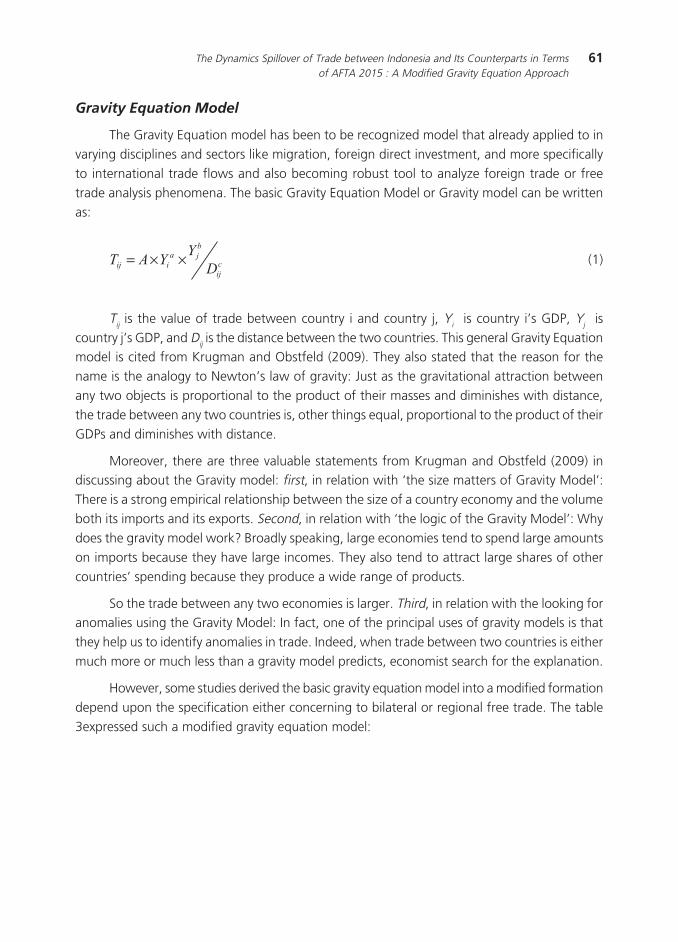
61The Dynamics Spillover of Trade between Indonesia and Its Counterparts in Termsof AFTA 2015 : A Modified Gravity Equation Approach
Gravity Equation Model
The Gravity Equation model has been to be recognized model that already applied to in
varying disciplines and sectors like migration, foreign direct investment, and more specifically
to international trade flows and also becoming robust tool to analyze foreign trade or free
trade analysis phenomena. The basic Gravity Equation Model or Gravity model can be written
as:
(1)
Tij is the value of trade between country i and country j, Yi is country i’s GDP, Yj is
country j’s GDP, and Dij is the distance between the two countries. This general Gravity Equationmodel is cited from Krugman and Obstfeld (2009). They also stated that the reason for the
name is the analogy to Newton’s law of gravity: Just as the gravitational attraction between
any two objects is proportional to the product of their masses and diminishes with distance,
the trade between any two countries is, other things equal, proportional to the product of their
GDPs and diminishes with distance.
Moreover, there are three valuable statements from Krugman and Obstfeld (2009) indiscussing about the Gravity model: first, in relation with ‘the size matters of Gravity Model’:
There is a strong empirical relationship between the size of a country economy and the volume
both its imports and its exports. Second, in relation with ‘the logic of the Gravity Model’: Why
does the gravity model work? Broadly speaking, large economies tend to spend large amounts
on imports because they have large incomes. They also tend to attract large shares of other
countries’ spending because they produce a wide range of products.
So the trade between any two economies is larger. Third, in relation with the looking foranomalies using the Gravity Model: In fact, one of the principal uses of gravity models is that
they help us to identify anomalies in trade. Indeed, when trade between two countries is either
much more or much less than a gravity model predicts, economist search for the explanation.
However, some studies derived the basic gravity equation model into a modified formation
depend upon the specification either concerning to bilateral or regional free trade. The table
3expressed such a modified gravity equation model:
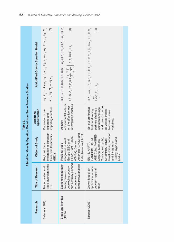
62 Bulletin of Monetary, Economics and Banking, October 2012
�������
�� �!����!�"��#��$��% ������ �!�������������&��#�� ���� !���
%�����&
)��
����
$%&
*'(
� ������%�����&
'()� ����� ���
��� ����
����� ��
���������*��+ ���,�� ��������
����
���
��� �
���
�����
��
����
��
��+
��
��
��"
���
����
�� �
��"�
�� �
� �
���
����
��
����
� �
���
���
��$�
��
(
1��
����
��
��+
���
���� �
"��
� �
���� �
"��
���� �
�$2
(
)��
���
��/
����
�$%
&34(
���
���
� �
��"�
�� �
���
��"
����
���#
����
���
�"�
����
����
���
����
����
����
����
����
���
���
���
��� �
���
����
�
��"
���
����
�� �
��"�
�� �
� �
5��
��
����
�$�
��
���
���!
(#�
����
����
�$�
/�
!(#�
������
!�
�� �
��$�
!�
/(��
�6�
� �!
���
���
$6!��
!(
!��
����
���
����
����
��
���
���
�+�
��
�� �
����
��
���
"���
��
��� �
����
7��
����
$28
89(
:��
� ��
/��
����
���
�� �
�� �
���
����
���
�.��
���
" ��
����
���
�,
%4#
;!
��!
#�
!�
0�<
/#�
!�
/#
!;
=�
���#
/!
:�
�)
$!�"
�� �
#/��
����
#��
� �
�#�
��6
�� �
(#/
!�
��
�>
$�
"���
#0�
����
#?��
���#
6��
����
���
���
�(#�
�+��
���-
��#�
����
���
�/
����
���
���
���
���
�� �
�����
���
�����
�"
������
���
+�� �
"�
���
���
���"
��"�
���
���
���
���
���
��.
����
�����
�"
����
���
���
��
��� �
����
@
$9(
$A(

63The Dynamics Spillover of Trade between Indonesia and Its Counterparts in Termsof AFTA 2015 : A Modified Gravity Equation Approach
The effect of the existence of some modified gravity equation models from previous
stand point allows rich analysis due to the dynamics of trade. This table below describes the
interpretation directly to coefficients of the modified model:
������'&���������������(��������������!�������&��#�� ���� !���
�������� ���
����� 1����#��@��$288&(
�&�������� ����-� ����� � ��
0�+���� � ������������ ����� � ���"�� ��#�+�������+������ ����� �"�������+����+������� �������
1��+������1 �����$2883( ���������+�����:=1��:=1������ ������+�� ���������+�.��� � �������"�� ����� � ���� "�������� ����
�+������������ ������+�"��� ����� ������������+���+����"���+�� ����+����-�������� ��� ������+��������+����-���$��.������������(#�+����"���+� ������� ��+���������������
7������$2889( !+ "+������ ����� ��+������� �"������� �� ������+ "+������������� ��#.+ �+ ���������+���� ��� � ���"������������@�+�������+���� � ��� ���������������� � ��
!+ "+����� ����� ��+� ����� �"���������""����+ "+�� ������@���+���� � ���� ���������������� � �����
�+���� � ������ ������������� ����+�����������������"�� ��������� � ����� "���#������ �"��.+��+�� �+��������������� ����$������� ������(��.+��+���� "�������������������+���������������$������ ��������(
�+���� � �����+� �������������� ��#����+������� "����� "�#��� � ����������
�+�� ��������� � ��� ���������������"�� ��� ��� � ��������������� �������������
��� � ��$%&&&( = ������+���� "� ������"�� ��������� ��������������# ����������������������$� -������������ ����������� ��� ��(���� -����� �������. �+� ������
��� ���� ��� ��+� ����� �"������ ������������+������"�� ��# �� "� ����#������������� ����+��������� ��
:=1���������� ��#���+���+��+���#+���� "� ������� � ���������� ��������������
)�������/�����$%&34( �+� ��������������� ����� �������������� �+����� �"������ ������.��������������@� ���"������������� � ������� ����� ������������ �����# ��� ��� � ���� ��� �������� �� �� ��� � ��
6��"������� ��+�������� ���� ��������� ������+����� ���"������������� ��������� �������.+ ������������� ������������������ �� �������+����������������������#��""��� �"�+����� � ���� ��+��������"�� ��
�+�������� ����+� ����� �"��������+����+������� � ���������+�������������#� �������"��������� ������ ���"������� � � ������������ ���� ���������� ��#����� �" ���������������. �+������ �"�������������"����+�������� ���������@/�������#����"����-���������������������������� �� �+���������� � �" ������ ����������� �+ �"���������� ��� ��� �����.��-@�+����� � ���� ��+��������� � ��

64 Bulletin of Monetary, Economics and Banking, October 2012
III. METHODOLOGY
This paper proposed a Modified Gravity Equation model such following equation:
(5)
(6)
(7)
(8)
Where
- ΣTBij is sum value of trade balance (net exports) of rubber based-products, wood based-
products, agro based-products, and fisheries from Indonesia (i) to other selected ASEAN
members (j) in US Dollar;
- α1 is constant or unobserved effect;
- Yit , Yjt are GDP per capita of Indonesia and other selected ASEAN members GDP per capitain US Dollar
- Dij is distance between Indonesia capital city (i) and other selected ASEAN members capital
city (j) kilometer;
- ti is Indonesia average CEPT rates (i) in percentage;
- tj is selected ASEAN members average CEPT rates (j) in percentage;
- exi is Indonesia real exchange rates (i) in per US Dollar;
- exj is selected ASEAN members average CEPT rates (j) in per US Dollar;
- eij is lognormal error term.

65The Dynamics Spillover of Trade between Indonesia and Its Counterparts in Termsof AFTA 2015 : A Modified Gravity Equation Approach
The data of the examination retrieved from International Trade Centre2 that containing
the data of trade balances. Then, data of the GDP per capita plus the CEPT, the distance, and
real exchange rates are compiled from ASEAN and other sources3, and International Financial
Statistic 2009, respectively. The time period all of the data are from 2002 to 2008.
This paper estimates and giving an analysis tothe importance of the coefficient magnitude.
First, a high level of income in the exporting country indicates a high level of production. Thus,
it increases the abundant ofgoods to export. The notion of α2 denotes to bepositive (+) andmight be interpreting as whether the absorption effect or the role of play within the free trade
zone. Second, the notation of α3 is also expected to be positive (+) since a high level income in
the importing country suggests higher imports and also connected to the four primary option
i.e. the absorption effect orthe scale of economies orthe natural comparative advantage, and
or the role of play. Third, , , , , the distance parameters of α4 is a positive (+) since it is a proxy of all
possible trade costs and also positive related to efficient trade costs. Distance has a significantnegative effect on bilateral exports, in part because trade costs (such transportation and
communication) are likely to increase with distance or vice versa.
Fourth, the notation of α5 occurs as a positive (+) sign in which Indonesia induces lowering
the cost of import (ACEPT rate) instead of selected members. In this context, Indonesia can be
defined as an importer and therefore can be associated with a trade creation strategy. A trade
creation policy signifies to gain much beneficial from free trade. Fifth, the coefficient of α6
notes to possess negative (+) sign and hence, the Indonesia cost of export (ACEPT rate) can be
lower compared to selected members. Thus, it can be inferred that Indonesia allows to strategy
of a trade creation. Sixth, it is expected that the notion of α7 denotes negative (-) sign and
however for the parameter of α8 is estimated to be positive (+). Both of which indicates that
Indonesia Rupiah (IDR) undervalued over selected members currency. As a consequence,
Indonesia trade balance increases constructively because its products are definitely cheaperthan other competitor products.
Furthermore, this paper will utilize Pooled Least Square (PLS) method therefore panel
data or pooled data within pooling in time series and cross-sectional observations or combination
of time series and cross-section data (Gujarati and Porter, 2009). Then Gujarati and Porter
(2009) elaborate the advantages of panel data over just cross section or just time series data:
first, by combining time series of cross section observations, panel data gives more informativedata, more variability, less collinearity among variables, more degrees of freedom and more
efficiency. Second, by studying the repeated cross section of observations, panel data are
better suited to study the dynamic of change. Third, panel data can better detect and measure
effects that simply cannot be observed in pure cross section or pure time series data. Fourth,
panel data enables us to study more complicated behavioral models.
2 Downloadable at www.trademap.org.3 Available at www.asean.org, www.indo.com/distance and www.geobytes.com/citydistancetool.htm.

66 Bulletin of Monetary, Economics and Banking, October 2012
Pooled Least Square (PLS) regression or Constant Coefficients Model is assumed that
explanatory variables (independent variables) are non stochastic. If they are stochastic, they are
uncorrelated with the error term. Sometimes it is assumed that the explanatory variables are
‘strictly exogenous. A variable is said to be strictly exogenous if it does not depend on current,
past, and future values of the error term (Gujarati and Porter, 2009). It is also assumed that the
error term is eij ~ idd (0,σ2e) that is, it is independently and identically distributed with zero
mean and constant variance and also may be assumed that error term is normally distributed.
The outcomes of PLS will provide two estimations as a baseline to analyze Indonesian
multilateral trading counterparty: first, prob. (t-stat) or t test or testing hypothesis about any
individual partial regression coefficient, particularly for explanatory variables towards dependent
variables. Linkage to the hypothesis testing, this paper employs if the ρ-value or prob. (t-stat) is
less thanany level of significance α at 1%, 5%, or 10 %, automatically the null hypothesis is
rejected. It implies the independent variables are partially affectedby the dependent variables(Gujarati and Porter, 2009). These estimations have a function to make prominent interpretation
of each parameter related to reveal trade pattern.
Second, the adjusted R2, is a descriptive measure of the strength of the regression
relationship, a measure of how well the regression line fits the data (Aczel, 1995). Moreover,
Aczelmentions that the requirement of an indication of the relative fit of the regression model
to the data such R2 value of 0.9 or above is very good, a value above 0.8 is good, a value of 0.6or above may be satisfactory, a value of 0.5 or below maybe poor. However, referring to Aczel,
this paper proposes different criteria due to utilization of the adjusted R2. The interval valueof
the adjusted R2 ranges from 0 % to 25 %; 26 % up to 50%; and 51% to 100 % imply as a
poor sector of Indonesia, as a weak sector for Indonesia and as a strength sector for Indonesia
respectively.
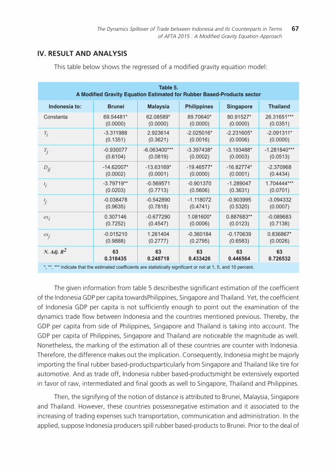
67The Dynamics Spillover of Trade between Indonesia and Its Counterparts in Termsof AFTA 2015 : A Modified Gravity Equation Approach
IV. RESULT AND ANALYSIS
This table below shows the regressed of a modified gravity equation model:
������)�� �!����!�"��#��$��% ��������������!�����* ���������!+&��! ����������
-�������� �.
���������
B#BB#BBB �� �����+���+���� �������� � ����������� �� ������ "� �����������%#4#���%8�������@
����� ������� �&������ �������� �&�����
*&@4AA3%B$8@8888(
*2@8343&B$8@8888(
3&@'8*A8B$8@8888(
38@&%42'B$8@8888(
2*@9%*4%BBB$8@894%(
�� 9@9%%&33$8@%94%(
2@&29*%A$8@9*2%(
2@8248%*B$8@88%*(
2@29%*84B$8@888*(
2@8&%9%%B$8@8888(
�� 8@&988''$8@*%8A(
*@8*9A88BBB$8@83%&(
9@9&'A93B$8@8882(
9@%&9A33B$8@8889(
%@23%3A8BBB$8@84%9(
��� %A@*288'B$8@8882(
%9@*9%*&B$8@888%(
%&@A*4''B$8@8888(
%*@32''AB$8@888%(
2@9'8&*3$8@AA9A(
�� 9@'&'%&BB$8@8289(
8@4*&4'%$8@''%9(
8@&8%9'8$8@4*8*(
%@23&8A'$8@9*9%(
%@'8AAAABBB$8@8'8%(
�� 8@893A'3$8@&*94(
8@4A23&8$8@'3%3(
%@%%38'2$8@A'A%(
8@&89&&4$8@4928(
9@8&A992$8@888'(
��� 8@98'%A*$8@'242(
8@*''2&8$8@A4A'(
%@83%*88B$8@888*(
8@33'*39BB$8@8%29(
8@83&*39$8@'%93(
��� 8@8%42%8$8@&333(
%@2*%A8A$8@2'''(
8@9*8%3A$8@2'&4(
8@%'8*9&$8@*439(
8@39*3*'B$8@882*(
��������� /"01"�2#"$
/"01!#23�2
/"01#""#!/
/"01##/$/#
/"013!/$"!
The given information from table 5 describesthe significant estimation of the coefficient
of the Indonesia GDP per capita towardsPhilippines, Singapore and Thailand. Yet, the coefficient
of Indonesia GDP per capita is not sufficiently enough to point out the examination of thedynamics trade flow between Indonesia and the countries mentioned previous. Thereby, the
GDP per capita from side of Philippines, Singapore and Thailand is taking into account. The
GDP per capita of Philippines, Singapore and Thailand are noticeable the magnitude as well.
Nonetheless, the marking of the estimation all of these countries are counter with Indonesia.
Therefore, the difference makes out the implication. Consequently, Indonesia might be majorly
importing the final rubber based-productsparticularly from Singapore and Thailand like tire forautomotive. And as trade off, Indonesia rubber based-productsmight be extensively exported
in favor of raw, intermediated and final goods as well to Singapore, Thailand and Philippines.
Then, the signifying of the notion of distance is attributed to Brunei, Malaysia, Singapore
and Thailand. However, these countries possessnegative estimation and it associated to the
increasing of trading expenses such transportation, communication and administration. In the
applied, suppose Indonesia producers spill rubber based-products to Brunei. Prior to the deal of
68 Bulletin of Monetary, Economics and Banking, October 2012
trade, Indonesia producers will take place 14.6% from the overall transaction as the trade
expenses. This paper found that the most costly of trading goes to Philippines by 19.5%.
The estimation of notation ti and tj explore the tariff ACEPT exercising. The significance
ACEPT is featuring between Indonesia and Thailand. However, this featuring only focuses to
Indonesia ACEPT which is lowering 1.7% than Thailand. The information of previous deduces
that Indonesia as an importer country may allow to implement a trade creation strategy. This
strategy imposes the beneficial for Indonesian consumer therefore enjoying the importing rubberbased-products due to relative cheaper price tag rather domestic rubber based-products. Thus,
yet, Indonesia producers are loss by 1.7% in response to imported finished goods. The
advantageous only occur once Indonesian producers are taking crude and intermediated goods
into account of import. By that implementation, Indonesian producers can be saving the money
up to 1.7%. In contrast, Indonesia government as the third party definitely possesses the
falling tariff revenue about 1.7%.
The estimation of the notation Thailand Bath (THB) implies the magnitude and in contrast
with the Indonesia Rupiah (IDR). Consequently, if the THB is appreciating over IDR by then it
might be elevating the Indonesia net export to around 0.83% or vice versa. Furthermore, the
important information is containing within the table 5 is the estimation of theadjusted R2 in
which reflecting the grading of rubber based-products sector comparing Indonesia to selected
ASEAN members. This paper found that Indonesia incurs rubber based-products as a strengthcommodity to trade with Thailand (72.65%). Nevertheless, the rest indicates not strategically
to make significant trade therefore the weak and the poor estimation of adjusted R2.
The following table 6 depicts two effects regarding the GDP per capita estimation. First,the significance estimation and the positive sign of Indonesian GDP per capita indicate that
Indonesia directly exports magnitude wood based-products to Brunei. Second, in the similar
significance but with the negative sign of Indonesian GDP per capita assures that Indonesiaallow to open import of rubber based-products from Malaysia, Philippines, Singapore, and
Thailand.It is a plausible finding that Indonesia is not strictly riveted to push its export to these
countries. As a suggestion that it might explicable that importing from these countries is only
beneficial forthe wood based-products in form of whether of crude or intermediated goods in
order to process of each or both to be an added value rubber based-products. Later on, the
added value goods can be spilled out to the non-member of AFTA such Europe, USA, Japan,India and China. The strategy of this is useful to lift much more trade surplus.Concerning to the
trade cost by the parameter of distance, it reveals that the highest trade cost places to Philippines
because of taking about 14.3% into expenses from the total deal of transaction.
In the case of the cost of import, Indonesia versus Malaysia has the same significance
estimation. The table 6 exhibits that Malaysia actuallyimposes highercost of import (ACEPT)
compared to Indonesia. By this condition, Indonesia may apply the strategy of trade diversion
or trade creation. To address the trade diversion, Indonesia is acted as an exporter. Consequently,

69The Dynamics Spillover of Trade between Indonesia and Its Counterparts in Termsof AFTA 2015 : A Modified Gravity Equation Approach
Indonesia producers are relatively loss on exporting to Malaysia by 2.84% therefore facing
ahigher tariff. In response to this, Malaysia producers may increase their price the same as the
wood based-products from Indonesia. And the surplus is gained by Malaysia worth 2.84%.
Nevertheless, the Malaysia consumers indicate loss up to 2.8 % and in oppose with the
government where enjoying the tariff revenues to around 2.8%.
How about the Indonesiaasimporter in this case? Automatically it mainly applies thetrade creation. The effects of a trade creation are smoothly advantageous for Indonesia
consumersnot to mention Indonesia producers. Indonesia consumers relatively satisfied to
consume cheap wood based-products from Malaysia. Indonesia producers in related to further
processing will accept discount to around 2.9 % by importing in form of raw materials and
semi finished-goods. If the exchange rate of IDR is defined appreciating against Philippines
Peso (PHP) therefore it might potentially underminethe value of the Indonesia net export interms of the wood based-products to approximate 0.5 %. The estimation of adjusted R2 identifies
Malaysia (67.7%), Philippines (66.95), Singapore (around 60%) and Thailand (57.7%) as the
importance partners for the Indonesia trade flows under the scheme of AFTA. It implies these
countries possibly generate high volume of trading with Indonesia regarding the wood based-
products.
������,�� �!����!�"��#��$��% ��������������!�����-��!�����!+&��! ����������
-�������� �.
���������
B#BB#BBB �� �����+���+���� �������� � ����������� �� ������ "� �����������%#4#���%8�������@
����� ������� �&������ �������� �&�����
2'@&8&&8$8@%%92(
4&@***AAB$8@8888(
43@2%A89B$8@888%(
A%@'&8A9BB$8@8%9*(
A3@%3'9*BB$8@8%'A(
�� &@%3**92B$8@8883(
'@A348'3B$8@8888(
2@3A%'83B$8@8888(
2@44&'%%B$8@888A(
2@**832*B$8@8882(
�� A@8434BBB$8@8*22(
9@8'*3%3B$8@8884(
%@2249*&$8@%A94(
%@4%'3'4$8@%892(
%@'9&%3ABBB$8@8&3&(
��� A@229*'&$8@92'8(
%8@33A%9B$8@888A(
%A@A9'**B$8@8888(
%8@%38%8BB$8@8%&4(
%2@22A22BB$8@8%'8(
�� A@%2%3A3BB$8@89%8(
2@3&4%&9BB$8@8*A&(
2@&'%%93BBB$8@84*&(
%@A%82'4$8@9*3'(
8@93&A4'$8@'&A8(
�� 8@89&A*4$8@&*3%(
2@39'4&'BBB$8@8'2&(
2@A&42%9$8@%%84(
8@&&232%$8@4942(
8@&%*A%4$8@48&9(
��� 2@&*'99AB$8@884A(
9@9%8338B$8@8888(
%@*22A89B$8@8888(
%@94&392B$8@8883(
%@432&48B$8@8882(
��� 9@23A83*BB$8@8%22(
%@4'A9%8B$8@8888(
%@%2AA9AB$8@88%2(
%@8898''BB$8@8222(
%@2*''3&B$8@88AA(
��������� /"01##!2$2
/"01/33�"3
/"01//4#$/
/"01$4/#"3
/"01$33"3�

70 Bulletin of Monetary, Economics and Banking, October 2012
With respect to GDP per capita as one ofthe primary variable, the table 7shows the
significance estimationfor Indonesia, Philippines, Singapore and Thailand. Nonetheless, thesymbol of GDP notation for each country is a negative. It implies between Indonesia and these
countries as mentioned from pervious statement have strong trade flows each other. Consider
Indonesia to Singapore, Indonesia might be imported by around 4.43% of finished agro based-
products from Singapore to fulfill the domestic consumption. Indonesia is taking the percentage
of 3.1% from the total production of Indonesia agro based-products into account of export to
Singapore. The material of export could be a lot of portion of raw material whether to processor to consume by Singapore.
Furthermore, the Philippines is identifying as the most expensive country cost of related-
trading. Therefore, the Indonesia producers are suggested to provide a special budget to treat
the trade expenses to Philippines as percentage of 25.68% from the total transaction. Table 7
also contains the information due to the cost of import (ACEPT). Nevertheless, none the country
reveals the significance estimation. By that, there is no more analysis relate to this parameter.This paper found the significance estimation exchange rate of IDR against Malaysia Ringgit
(RMY). Once IDR is appreciated to RMY, Indonesia’s trade balance of agro based-products is
probably deficit up to 0.48%. The notation of the adjusted R2 is summarized that all the
selected members as Indonesia partner of trading denote there are a huge transaction in AFTA
in terms of agro based-products.
������.�� �!����!�"��#��$��% ��������������!��������������!+&��! ����������
-�������� �.
���������
B#BB#BBB �� �����+���+���� �������� � ����������� �� ������ "� �����������%#4#���%8�������@
����� ������� �&������ �������� �&�����
42@84948B$8@88%%(
*'@94*4AB$8@8888(
%28@2&A2B$8@8888(
%83@48'2B$8@8888(
*'@9&%&AB$8@8888(
�� A@393*8BBB$8@899A(
%8@8499&B$8@8893(
9@239''AB$8@8888(
9@%89398B$8@8888(
2@&2938%B$8@8888(
�� 3@9'*8*%B$8@8888(
*@A''9A%BBB$8@8'A8(
A@*9A*42B$8@8888(
A@A2'249B$8@8888(
2@&*949&B$8@8882(
��� &@9*439BB$8@8%AA(
%A@'229'B$8@888%(
24@*3*&AB$8@8888(
22@*%8%&B$8@8888(
%%@329*&B$8@88%*(
�� 9@'*%9*BB$8@8299(
8@9%*A&*$8@3'*4(
8@24%&'8$8@34*'(
%@*A23'3$8@293&(
8@*2%2&'$8@4*%'(
�� 8@984282$8@'28*(
%@38**43$8@9''%(
%@&A9939$8@%'8&(
8@*2'333$8@*4'&(
2@22%&3*BB$8@82&%(
��� 9@24233%B$8@888*(
2@'&&A2*B$8@88A9(
%@48AA22B$8@8888(
%@9%3*82B$8@8889(
8@*89*'9BB$8@89*'(
��� 4@223%24B$8@8888(
2@983%38BBB$8@84&2(
8@A844&A$8@%'3*(
8@A39AA'$8@2848(
%@2%2%%&B$8@8882(
��������� /"01/030#3
/"01$##4#!
/"013#�#23
/"0130�!/$
/"0134$"3!

71The Dynamics Spillover of Trade between Indonesia and Its Counterparts in Termsof AFTA 2015 : A Modified Gravity Equation Approach
Table 8 given information about the significance of GDP estimation for all members
without Brunei. To the extent of the significance GDP estimation, in case Indonesia against
Philippines conveys an examination that since Indonesia possesses the negative notation therefore
Indonesia implies as an importer. So that it allows Philippines to convey its fisheries to Indonesia
by around 4.5% from its total capacity. Surprisingly, there is a surplus transaction cost related-
trade to Brunei, Malaysia, and Singapore. It might be these countries producers pro active tosend the crew to take away fisheries products live from Indonesia.
It is noticeable that only between Indonesia and Thailand induce the significance estimation
of notation tariff of trade. Moreover, from the regressed result that the negative sign incurs
the lower Indonesia tariff than Thailand. Hence, it is suggested more suitable being an importer
and more properly utilizing a trade creation strategy to face Thailand. Thus, Indonesia producers
might be decreased up to 3.5% in order to equally their price with the price of final product of
fisheries from Thailand. Unless for raw and intermediated goods, the Indonesia producers mayenjoy the surplus therefore the lower price from Thailand. The Indonesia consumers are having
the surplus up to 3.5% whether fisheries from domestic or from Thailand. However, Indonesia
government linkages to the tariff revenue from the fisheries of Thailand Indonesia government
slightly fall by around 3.5%.
Regarding exchange rate between Indonesia and Malaysia, the IDR indicates appreciated
over the RMY and as a consequence may affecting the decreasing of Indonesian net export on
fisheries by about 1.11%.
������/�� �!����!�"��#��$��% ��������������!��������������������
-�������� �.
���������
B#BB#BBB �� �����+���+���� �������� � ����������� �� ������ "� �����������%#4#���%8�������@
����� ������� �&������ �������� �&�����
4A@%3&2'B$8@8888(
92@'*433B$8@882'(
3@A3294&$8@A2A&(
22@329A%BB$8@8*99(
A@9*9*43$8@'&*4(
�� 3@A*249*B$8@8888(
%2@%A92'B$8@8888(
2@&%%34AB$8@8888(
9@89922%B$8@8888(
2@493'*3B$8@888%(
�� 8@&449*%$8@A'A*(
%'@9*48AB$8@8888(
A@A*3222B$8@8888(
A@&*8A9*B$8@8888(
A@*8%%%8B$8@8888(
��� %8@83929B$8@888A(
4@AA93'8BBB$8@89*4(
2@*A'84A$8@2&*&(
*@9%3'9%BB$8@8A*&(
2@8A8A&'$8@*99'(
�� A@4&%A8%B$8@8882(
8@3&8A2%$8@44*4(
8@2*&%A9$8@32'A(
8@3&&9A2$8@A942(
9@494483B$8@88'&(
�� 8@4*&'''$8@94*9(
9@A2A29%BBB$8@82'9(
2@A&9AA%BB$8@8A&A(
2@'448&3BB$8@822*(
4@'48*3*B$8@8888(
��� %@922*&8BB$8@8A2*(
2@*4*4&'B$8@888A(
8@48*''9BB$8@894*(
8@%A2A99$8@*%84(
8@*28&84BBB$8@8'%'(
��� %@'8%884BB$8@894*(
9@''44AAB$8@888%(
8@8&2A3%$8@'2*4(
8@A39%98$8@%239(
8@A88'3A$8@2'38(
��������� /"013//#/
/"013�"!"2
/"013/2///
/"013/#2�3
/"01//!3!$

72 Bulletin of Monetary, Economics and Banking, October 2012
The adjusted R2 determines the degree of the fisheries trade between Indonesia and its
partner of selected member of AFTA. The value of adjusted R2 implies that each selected
country points out as a highly important to an intended objective for Indonesia in terms of
AFTA.
V. CONCLUSION
Overall, from the empirical standpoint of the dynamics finding indicates that the somenoted. The objective of trade flow is addressed to gain magnitude beneficial for Indonesia
nexus the AFTA. The beneficial can be come up ultimately from the factor of the natural
competitive advantage by employing GDP as a proxy of this factor. Actually, based on the
findingof estimation GDP, in as much, Indonesia might be concluded as the country which
exposing the strength of the natural competitive advantage instead of the others. Such sectors
are already mentioned in analysis on empirical findings and discussion. Next, the factor of thetariffs of free trade effect will relevant to in the applied of the strategy either a trade creation
or a trade diversion. Rely on both strategies, the rubber based-products sector, Indonesia may
implement a trade creation only to Thailand in order to gain from free trade.
On the wood based-products, Indonesia may utilize both trade creation and trade diversion
to Malaysiadepends upon which one is more beneficial for Indonesia. Nonetheless, nothing
gain can found from the tariff of trade linkage to agro-based products. Once again Thailand isbecome an advantageous partner for Indonesia in terms of fisheries sector. Indonesia may
apply the trade creation in order to bolster the volume of trade with Thailand. The finding of
the adjusted R2 might interpret as a whole by doing such free trade with particular selected
ASEAN member, Indonesia is expected to earn the greater amount of surplus. Hence, for the
rubber based-products sector, Indonesia may direct its trade flows more concerning to Thailand
rather than others. In the context of the wood based-products, Brunei is exclusion but the restis strategic for Indonesia. For instance, Indonesia should extensively engage of trading with
each selected members regarding the agro based-products sector and the fisheries sector.
By and large, this paper suggests that if Indonesia has a goal being the key player in the
foreseeable AFTA therefore Indonesia should rocketed its infrastructure to back up its trade
and then increasing sharply its GDP per capita, minimizing the trade barrier and cost, and
managing the exchange rates as well. Hereafter, the relative beneficial can be aimed by Indonesiaaccording 2015.
NoteNoteNoteNoteNote: please put the panelist comment for future studies here.

73The Dynamics Spillover of Trade between Indonesia and Its Counterparts in Termsof AFTA 2015 : A Modified Gravity Equation Approach
REFERENCES
Aczel, D., AmirAczel, D., AmirAczel, D., AmirAczel, D., AmirAczel, D., Amir, (1995),Statistics Concepts and Applications, Irwin.
ASEAN Economic Community BlueprintASEAN Economic Community BlueprintASEAN Economic Community BlueprintASEAN Economic Community BlueprintASEAN Economic Community Blueprint. “ASEAN Secretariat”, Jakarta, January 2008.
ASEAN Economic Community ChartbookASEAN Economic Community ChartbookASEAN Economic Community ChartbookASEAN Economic Community ChartbookASEAN Economic Community Chartbook. “ASEAN Secretariat”, Jakarta, September, 2009.
ASEAN. “ASEAN. “ASEAN. “ASEAN. “ASEAN. “ASEAN Free Trade Area (AFTA Council)”http://www.asean.org/19585.htm., October
2010.
Balassa, BelaBalassa, BelaBalassa, BelaBalassa, BelaBalassa, Bela. “Trade Creation and Trade Diversion in the EEC”, Economic Journal, No. 77, p1-
21, 1967.
Brada, Josef C and Mendez, Jose ABrada, Josef C and Mendez, Jose ABrada, Josef C and Mendez, Jose ABrada, Josef C and Mendez, Jose ABrada, Josef C and Mendez, Jose A. “Economic Integration Among Developed, Developing
and Centrally Planned Economies : A Comparative Analysis”, The Review of Economics andStatistics, 1985.
Calvo-Pardo, Hector., Freund, Caroline., and Ornelas, EmanuelCalvo-Pardo, Hector., Freund, Caroline., and Ornelas, EmanuelCalvo-Pardo, Hector., Freund, Caroline., and Ornelas, EmanuelCalvo-Pardo, Hector., Freund, Caroline., and Ornelas, EmanuelCalvo-Pardo, Hector., Freund, Caroline., and Ornelas, Emanuel. “The ASEAN Free Trade
Agreement: Impact on Trade Flows and External Trade Barriers”. Policy Research Working
Paper The World Bank Development Research Group Trade and Integration Team, 2009.
Dodge, DavidDodge, DavidDodge, DavidDodge, DavidDodge, David. “Economic Integration in North America”, Bank of Canada Review, 2003.
El-Agraa, Ali MEl-Agraa, Ali MEl-Agraa, Ali MEl-Agraa, Ali MEl-Agraa, Ali M, (1997), Economic Integration Worldwide, St Martins Press, New York.
Gujarati, N., Damodar and Porter, C., DawnGujarati, N., Damodar and Porter, C., DawnGujarati, N., Damodar and Porter, C., DawnGujarati, N., Damodar and Porter, C., DawnGujarati, N., Damodar and Porter, C., Dawn, (2009), Basic Econometrics, Fifth Edition,
McGraw-Hill International Edition.
Husted, Steven and Melvin, MichaelHusted, Steven and Melvin, MichaelHusted, Steven and Melvin, MichaelHusted, Steven and Melvin, MichaelHusted, Steven and Melvin, Michael, (2010),International Economics, Eight Edition, Addison-Wesley.
Indonesian and Bali on the netIndonesian and Bali on the netIndonesian and Bali on the netIndonesian and Bali on the netIndonesian and Bali on the net.http://www.indo.com/distance, October 2010.
Krugman, Paul R. and Maurice ObstfeldKrugman, Paul R. and Maurice ObstfeldKrugman, Paul R. and Maurice ObstfeldKrugman, Paul R. and Maurice ObstfeldKrugman, Paul R. and Maurice Obstfeld, (2009), International Economics: Theory and Policy,
Eight Edition, Addison-Wesley.
Market Analysis and Research, International Trade CenterMarket Analysis and Research, International Trade CenterMarket Analysis and Research, International Trade CenterMarket Analysis and Research, International Trade CenterMarket Analysis and Research, International Trade Center. “Trade Map” http://
www.trademap.org/selectionmenu.aspx, October 2010.
Pacheco, Amurgo., Alberto and Pierola, Denisse., MarthaPacheco, Amurgo., Alberto and Pierola, Denisse., MarthaPacheco, Amurgo., Alberto and Pierola, Denisse., MarthaPacheco, Amurgo., Alberto and Pierola, Denisse., MarthaPacheco, Amurgo., Alberto and Pierola, Denisse., Martha. “Patterns of ExportDiversifcation
in Developing Countries: Intensive and Extensive Margins”. Policy Research Working Paper,4473, The World Bank International Trade Department, 2008.

74 Bulletin of Monetary, Economics and Banking, October 2012
Pelkmans, Jacques,Pelkmans, Jacques,Pelkmans, Jacques,Pelkmans, Jacques,Pelkmans, Jacques, (2006),European Integration: Method and Economic Analysis, Third
Edition,Pearson Education Limited.
Tamirisa, T., NataliaTamirisa, T., NataliaTamirisa, T., NataliaTamirisa, T., NataliaTamirisa, T., Natalia. “Exchange and Capital Controls as Barriers to Trade”. IMF working
paper, 1999.
Venables. J, AnthonyVenables. J, AnthonyVenables. J, AnthonyVenables. J, AnthonyVenables. J, Anthony. “International Trade; Regional Economic Integration”, The InternationalEncyclopedia of Social and Behavioral Sciences, Article 34), London School of Economics,
2000.
Zarzoso, Martines., InmaculadaZarzoso, Martines., InmaculadaZarzoso, Martines., InmaculadaZarzoso, Martines., InmaculadaZarzoso, Martines., Inmaculada.” Gravity Model: An Application to Trade Between RegionalBlocs”, Atlantic Economic Journal, 2003.
75Impact of Global Financial Shock to International Bank Lending in Indonesia
IMPACT OF GLOBAL FINANCIAL SHOCK TOINTERNATIONAL BANK LENDING IN INDONESIA
Tumpak Silalahi, Wahyu Ari Wibowo, Linda Nurliana 1
This study intends to determine whether a shock that occurred in developed countries, the source
of funding, was transmitted to Indonesia through international bank lending both directly and indirectly.
The methods used estimated the determinants of international bank lending. International bank lending
is one form of capital flows that have the potential for rapid reversal and that can lead to a financial crisis
as it has in the past. Understanding the determinants of bank lending is important as it can be used to
mitigate the impact of a financial crisis in the future. The empirical results showed that international bank
lending, either directly or indirectly, contributed to the Indonesian crisis. During the shock, Indonesia saw
global banking contract financing. It was also found that credit activities by foreign affiliates in Indonesia
saw acontraction in the country of the parent bank during the shock. However, it was found that the
bank lending by foreign affiliates, as joint ventures were more stable compared to the branch offices of a
foreign bank. In aggregate, international bank lending is affected by push and pull factors such as economic
growth (in developed countries and Indonesia), risk factors, and liquidity conditions, both in Indonesia
and globally. As for micro-banking models, other than the push and pull factors, the bank balance sheet
and other portfolio assets also affected bank lending activities to Indonesia.
Abstract
Keywords: Global Financial Shocks, Foreign Affiliates, International Bank Lending, transmission path,
dynamic panel.
JEL Classification: C33, E51, G15JEL Classification: C33, E51, G15JEL Classification: C33, E51, G15JEL Classification: C33, E51, G15JEL Classification: C33, E51, G15
1 The economic researchers at the Economic Research Group (GRE) Bank Indonesia wish to express appreciation to the GRE Chairman,Mr. Iskandar Simorangkir, and Mr. Ari Kuncoro and all the other researchers in the GRE. Thank you also to Mr. iweko Junianto for hishelp in the data collection process.
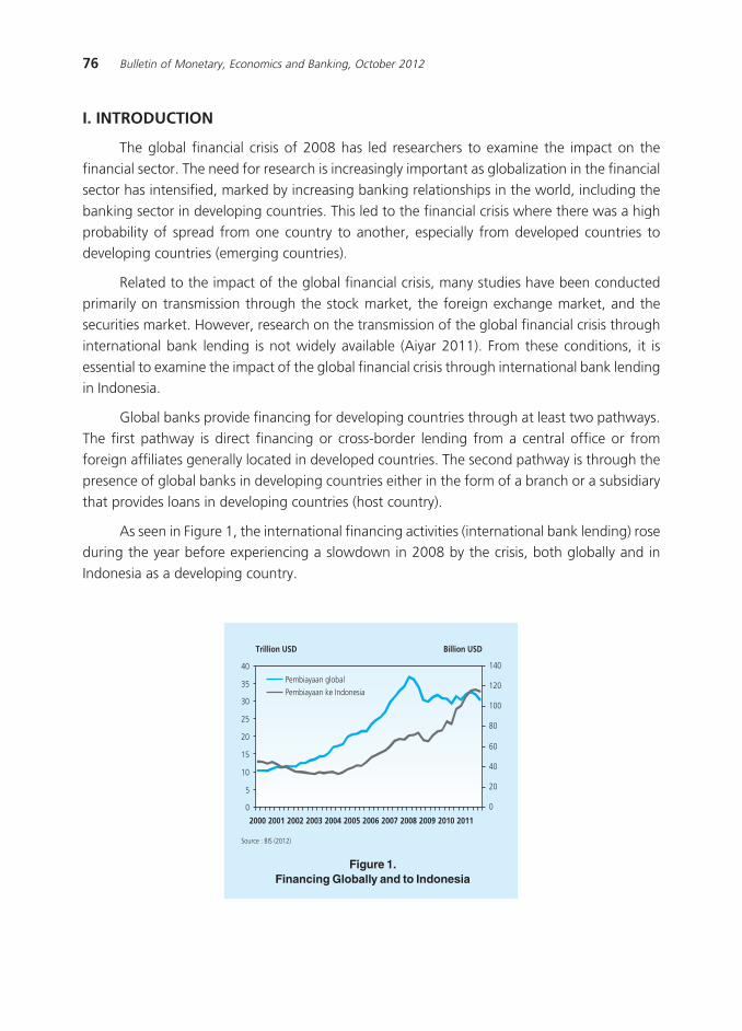
76 Bulletin of Monetary, Economics and Banking, October 2012
I. INTRODUCTION
The global financial crisis of 2008 has led researchers to examine the impact on the
financial sector. The need for research is increasingly important as globalization in the financial
sector has intensified, marked by increasing banking relationships in the world, including the
banking sector in developing countries. This led to the financial crisis where there was a high
probability of spread from one country to another, especially from developed countries todeveloping countries (emerging countries).
Related to the impact of the global financial crisis, many studies have been conducted
primarily on transmission through the stock market, the foreign exchange market, and the
securities market. However, research on the transmission of the global financial crisis through
international bank lending is not widely available (Aiyar 2011). From these conditions, it is
essential to examine the impact of the global financial crisis through international bank lendingin Indonesia.
Global banks provide financing for developing countries through at least two pathways.
The first pathway is direct financing or cross-border lending from a central office or from
foreign affiliates generally located in developed countries. The second pathway is through the
presence of global banks in developing countries either in the form of a branch or a subsidiary
that provides loans in developing countries (host country).
As seen in Figure 1, the international financing activities (international bank lending) roseduring the year before experiencing a slowdown in 2008 by the crisis, both globally and in
Indonesia as a developing country.
Figure 1.Financing Globally and to Indonesia
���������� ���������
������������ �� �
�
�
��
��
�
�
��
��
��
�
�
��
��
��
���
� �
���
���������������������������������� !���!
��� ��� �� ��� ��� ��� ��� ��� ��� ��� ��� ���
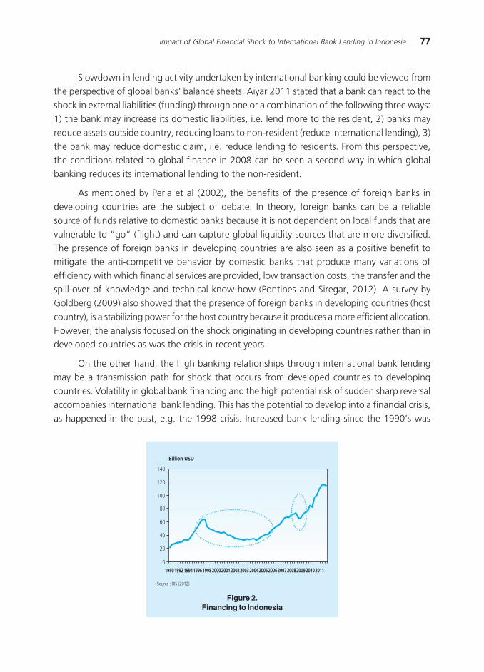
77Impact of Global Financial Shock to International Bank Lending in Indonesia
Slowdown in lending activity undertaken by international banking could be viewed from
the perspective of global banks’ balance sheets. Aiyar 2011 stated that a bank can react to the
shock in external liabilities (funding) through one or a combination of the following three ways:
1) the bank may increase its domestic liabilities, i.e. lend more to the resident, 2) banks may
reduce assets outside country, reducing loans to non-resident (reduce international lending), 3)
the bank may reduce domestic claim, i.e. reduce lending to residents. From this perspective,the conditions related to global finance in 2008 can be seen a second way in which global
banking reduces its international lending to the non-resident.
As mentioned by Peria et al (2002), the benefits of the presence of foreign banks in
developing countries are the subject of debate. In theory, foreign banks can be a reliable
source of funds relative to domestic banks because it is not dependent on local funds that are
vulnerable to “go” (flight) and can capture global liquidity sources that are more diversified.
The presence of foreign banks in developing countries are also seen as a positive benefit tomitigate the anti-competitive behavior by domestic banks that produce many variations of
efficiency with which financial services are provided, low transaction costs, the transfer and the
spill-over of knowledge and technical know-how (Pontines and Siregar, 2012). A survey by
Goldberg (2009) also showed that the presence of foreign banks in developing countries (host
country), is a stabilizing power for the host country because it produces a more efficient allocation.
However, the analysis focused on the shock originating in developing countries rather than indeveloped countries as was the crisis in recent years.
On the other hand, the high banking relationships through international bank lending
may be a transmission path for shock that occurs from developed countries to developing
countries. Volatility in global bank financing and the high potential risk of sudden sharp reversal
accompanies international bank lending. This has the potential to develop into a financial crisis,
as happened in the past, e.g. the 1998 crisis. Increased bank lending since the 1990’s was
Figure 2.Financing to Indonesia
���������
������������ �� �
�
�
��
��
��
���
� �
���
������� ������������ ��� ��� �� ��� ��� ��� ��� ��� ��� ��� ��� ���

78 Bulletin of Monetary, Economics and Banking, October 2012
followed by a sharp contraction of credit during the economic crisis in 1998 (Figure 2). The
sharp contraction lasted for a long period of time, i.e. up to the year 2004 with a contraction
of around 9% per year. Siregar and Choy (2010) stated that the impact of capital flows reversal
of the banking sector, in comparison of portfolio equity investment, was considered the main
cause of the deepening financial crisis in Asia in the late 1990’s.
After recovering from the 1998 crisis, in 2004-2007, the banks increased lending to
Indonesia. The importance of international bank lending as a source of financing in Indonesiacan be seen from the ratio of the annual GDP for Indonesia where the ratio ranged at 15%
(2004-2007). However, the increase was again followed by a decline during the economic
crisis of 2008.
Post-crisis bank lending contracted in 2008 to remind policy makers about the role of
global banks and international bank lending in transmitting the shock from developed to
developing countries. The increasing interlinkage between banks, the volatility risk, theaccompanying sudden capital reversal of leading global banks and the role of international
bank lending came to the attention of the IMF and the G-20 in its policy reform agenda in
2010 (Pontines and Siregar, 2012).
Several studies have been conducted to examine the behavior of global banks in developing
countries. Cetorelli and Goldberg (2009) found that international bank lending from global
banks with a high vulnerability to the USD, either directly or indirectly through foreign affiliates,declined during the global crisis. This may imply that international bank lending is a transmission
path of shock from developed to developing countries. Pontines and Siregar (2012), using a
sample of six developing countries in Asia found similar results. The shock from global banking
would reduce bank lending to developing countries (as Indonesia) where exposure (risk) is
increasing. Similarly, the behavior of foreign affiliates of global banking (i.e. branches) will
reduce lending in the host economy during a crisis, but not so with foreign bank subsidiaries.This condition occurs because foreign banks are locally incorporated subsidiaries in the host
country.
As the monetary and banking authority, Bank Indonesia needs to understand the
determinants of international bank lending to investigate the impact of capital flows to stabilize
the financial sector in Indonesia. This is because exposure to financing from developed countries
can be a transmission path of shock during times of financial turmoil in developed countries as
a source of financing. Siregar (2012) pointed out the failure to understand the relationshipbetween the bank (global and regional) that pose a risk to the consistency of macroeconomic
policy formulation and the ability to anticipate the effects of the financial sector weakness to
the country’s macroeconomic conditions.
It is important to understand the determining factors of international bank lending to
avoid or minimize welfare costs casued by disruption in international bank lending. Generally,
determinant factorsare analyzed in a framework of push and pull factors as mentioned by

79Impact of Global Financial Shock to International Bank Lending in Indonesia
Agenor (1998), Mody, Taylor and Kim (2001) and Ferrucci, Herzberg, Soussa and Taylor (2004).
Push factors refer to the determinants of global capital flows from the global financial
markets,and pull factors refer to specific elements in a country that reflect domestic fundamentals
and investment opportunities.
Considering the ongoing crisis in Europe and the potential for a prolonged crisis, the
study aims to look at the impact of the global crisis on international bank lending in Indonesia,
either directly via cross-border lending or indirectly through a representative bank in Indonesia(foreign affiliates). To determine the impact, the study identified the determinants of bank
lending to Indonesia, where one of the variables will represent a response to the global banking
system during the shock to this country against its lending activities of banks.
This study uses the most recent data that includes individual bank balance sheets aimed
to study the behavior of international banks in cross-border lending or via their foreign affiliates.
The sample in this study focused on a Foreign Bank Branch Office legal entities establishedunder foreign law and headquartered abroad and a mixed Bank Group (subsidiary) whose
shareholders are Foreign Banks and Domestic Banks.
Specifically, the first objective of this paper is to analyze the direct impact of the global
shock through the placement of international global bank lending to banks in Indonesia. The
second objective is to analyze the indirect impact of the global credit shock through foreign
affiliates operating in Indonesia.
The second section of this paper is the literature review. The third section discusses themethodology and the data used; while the fourth section presents the stylized facts and empirical
results. Conclusions and policy implications are given in the fifth section and closes the paper.
II. THEORY
2.1. Basic Approach
Modern Portfolio Theory (MPT)
Modern Portfolio Theory (MPT) is a theory in finance that attempts to maximize portfolio
expected return with a certain risk level or a way to minimize the risk to a certain level of
expected return done by selecting proportions of various asset choices. MPT is a mathematical
formulation of the concept of diversification in investing, where the aim of selecting a collectionof investment assets as a whole is lower than the risk of a single asset. This theory was first
introduced by Harry Markowitz (1952) which was further developed by James Tobin (1958) by
adding an asset that is risk-free to the analysis.
The underlying concept of MPT is that the assets in an investment portfolio should not be
selected individually based on their characteristics, but also should consider changes in asset
prices relative to prices of other assets in the portfolio. MPT defines risk as the standard deviation

80 Bulletin of Monetary, Economics and Banking, October 2012
Figure 3.Efficient Frontier
of the return, and models a portfolio as a weighted combination of the assets, so the return of
a portfolio is a weigthed combination of a return of assets in the portfolio. By combining assets
with returns that are not perfectly correlated, MPT seeks to lower the total variance of the
portfolio return.
MPT assumes that investors are risk averse, meaning where two portfolios that provide
the same expected return, investors will prefer a portfolio with a lower risk. So the investor
experiences higher risk if the compensation is greater for an expected return. Also, investorswho want a high expected return experience a higher risk.
The investor has two choices, such as a risky investment portfolio that has a higher rate
of return RA and variance , and a lower investment with returns RB and risks that are also
lower, variance . Investors can invest their funds with the proportion of ωA foraset-A and as
big as 1-ωA foraset-B, then expected return portfolio, Rp and risk portfolio is:
(1)
(2)
Where σA, σB is the standard deviation RAand RB, and is the correlation between RA and RB.
The combination portfolio that considers the relationship of risk (standard deviation) and
return is illustrated Figure 3 Efficient Frontier.
σ P2
σΑ2
σΒ2
"##�����$�%���$���
&��$�����'����!
(�� �������$#�!��
�$���������'����
)����#������$�
"*+��$���)�$���
Without the risk free asset, the red line is called efficient frontier. The lines represent the
entire portfolio that lies between the global portfolio with minimum variance and that has a
maximum return. A portfolio on this line had the lowest risk for a given level of return or the
highest rate of return with limited risk.

81Impact of Global Financial Shock to International Bank Lending in Indonesia
To find an optimal portfolio allocation (Figure 4) between investment A and B then use
capital market line MN which is a combination of return and risk of risky assets and no risk. The
slope of this line in equilibrium will touch the efficient frontier curve at the point P, which is a
combination of a portfolio that has a return RP and risk level . If investors want to gain a greater
return, then they should add to its investment portfolio a risky asset so that the risks become
greater or towards M point. Conversly, investors will earn a smaller return when holding aninvestment of smaller risk or move toward N.
Figure 4. Efficient Portfolio
������
�������
)&) )+
�
�
�
&
+
The number of optimal investment ωp* is obtained from the substitution equation (1)
and (2) with the slope (Rp - N) and slope as used by Miller (1971), and
we obtain:
σ P2
(3)
(3a)
(3b)
(3c)
where

82 Bulletin of Monetary, Economics and Banking, October 2012
Arbitrage Pricing Model (APM)
Financial theory was known to be part of scientific study since its introduction Sharpe
(1964) in the journal “Deriving Capital Asset Pricing Model (CAPM)”. The assumptions set out
in the CAPM theory is that the investor diversifies their asset portfolio for specific risk to the
portfolio. Further development of the theory of Capital Asset Pricing Model (CAPM) by Ross
(1976) added macroeconomic risks to the CAPM market risk variables known as the ArbitragePricing Model (APT Model)which is shown as follows:
(4)
Explanation of the model in question is the Expected Return of a portfolio of assets thatare affected by Risk Free Asset factors and the accumulation of all of the risk premiums from
unanticipated changes of risk bij which is the coefficient of risky assets and other assets.
Figure 5.CAPM and APM
���������� ������
���
���������
However, criticism of the theory of APM points to items not specified in the model of
macroeconomic factors such as interest rates, exchange rate risk, inflation or business cycle
fluctuations which become independent variables in determining the expected return of asecurity. Moreover, empirical evidence shows that the sensitivity of each security to different
macroeconomic changes are reflected in the factor loading bij.
Determinant Capital Flows
There is signifant literature that attempts to identify the main factors behind the increase
in the flow of funds to developing countries since the 1990s. Literature related to thedeterminants of capital flows to developing countries generally focus on two (2) groups of
factors: the pull and push factors (Agenor, 1998).
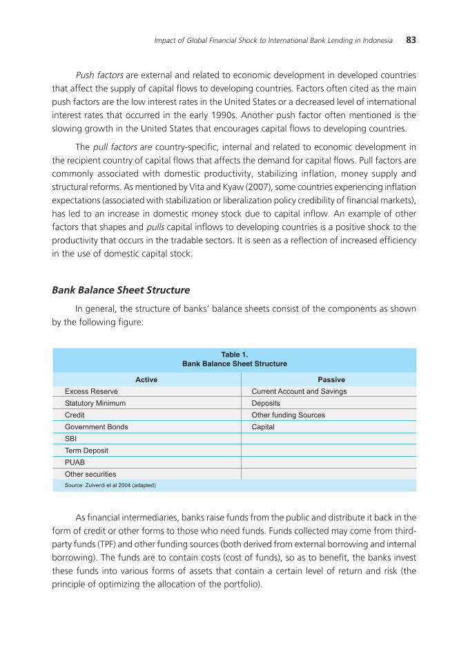
83Impact of Global Financial Shock to International Bank Lending in Indonesia
Push factors are external and related to economic development in developed countries
that affect the supply of capital flows to developing countries. Factors often cited as the main
push factors are the low interest rates in the United States or a decreased level of international
interest rates that occurred in the early 1990s. Another push factor often mentioned is the
slowing growth in the United States that encourages capital flows to developing countries.
The pull factors are country-specific, internal and related to economic development in
the recipient country of capital flows that affects the demand for capital flows. Pull factors arecommonly associated with domestic productivity, stabilizing inflation, money supply and
structural reforms. As mentioned by Vita and Kyaw (2007), some countries experiencing inflation
expectations (associated with stabilization or liberalization policy credibility of financial markets),
has led to an increase in domestic money stock due to capital inflow. An example of other
factors that shapes and pulls capital inflows to developing countries is a positive shock to the
productivity that occurs in the tradable sectors. It is seen as a reflection of increased efficiencyin the use of domestic capital stock.
Bank Balance Sheet Structure
In general, the structure of banks’ balance sheets consist of the components as shown
by the following figure:
������������ ����������� ���� �
������ ����
������������� ���������������� �������
��������� ���!�! "�������
��� �� #�$��%�� ����������
&�����!���'�� � �������
�'(
)��!"������
*+�'
#�$������������
��������������� ������������ ����
As financial intermediaries, banks raise funds from the public and distribute it back in the
form of credit or other forms to those who need funds. Funds collected may come from third-
party funds (TPF) and other funding sources (both derived from external borrowing and internal
borrowing). The funds are to contain costs (cost of funds), so as to benefit, the banks invest
these funds into various forms of assets that contain a certain level of return and risk (theprinciple of optimizing the allocation of the portfolio).
84 Bulletin of Monetary, Economics and Banking, October 2012
The forms of assets that may be an option for the bank to get a return are for example,
in the form of loans, government securities, money market or monetary instruments such as
SBI and term deposit (TD), as well as capital markets, etc. Zulverdi et al (2004) stated that all
banks face the problem of short-term liquidity management and are always working to optimize
the composition of the portfolio to generate maximum profit level. However, these efforts are
limited by the balance sheet constraint, where at any time the total assets must equal liabilities.
2.2. Global Crisis Effect on the Financial Markets
Research on the impact of the global shock to the financial sector in Indonesia has been
carried out and viewed from different apsects in the financial sector. Research by Kurniati et al.
(2008), examined the domestic financial market integration with global financial markets to
determine the impact of the global crisis on the domestic financial markets. Apsects observed
in the financial market included the market of stocks, bonds and foreign exchange. The studyconcluded that there is a correlation between the three financial markets in the country. By
using the standard deviation method, regression with error correction model approach, it was
generally found that the financial market in Indonesia is integrated with the global market,
though with different intensities.
The regression model used is as follows:
(5)Ri,t = i,t + i,t Rb,t + i,t
(6)
whereRi, t is the domestic stock price index and Rb is the benchmark index of global
share prices. Δ shows the difference of the variables. Regression results above show that the
global stock indices DJIA significantly affected the domestic stock price index (JCI). This significanteffect indicatesd that the domestic stock market is integrated with the global stock market. In
addition the share price, domestic determinants are estimated with an error correction model
with a long-term equation as follows:
JCI = f[DJIA, Earning Yield, Domestik Credit, Industrial Production, Capital Flows]
The estimates show that in the long-run, stock prices in Indonesia are affected by globalstock prices and the performance of public companies, while the fundamentals do not entirely
affect the stock price. The same model was also applied to the bond market and the foreign
exchange market.
In general, the stock market showed the highest intensity of integration where global
stocks significantly affected the movement of domestic stock. Meanwhile, a lower intensity
was found in the bond market due to relatively recent integration of the domestic bond market
with the global bond market. For the foreign exchange market, the integration is of a mixed

85Impact of Global Financial Shock to International Bank Lending in Indonesia
nature that occurs due to the movement of the dollar in the opposite direction of the global
currency. Thus, the effect of the crisis on the global markets most influenced the stock market
compared with other financial markets along with higher market integration with the global
stock market.
While the research of Dewati et al (2009) saw the changes of risk in financial markets at
times of crisis and changes in lending behavior of the banks. The risks studied were on the
bond market as represented by the Credit Default Swap (CDS) and the yield on governmentsecurities. The OLSmethodsto find the determinants that affect the CDS are estimated by the
following equation:
(7)CDS= f[D(ICRG), Volatility_IHSG,D(CADEV), D(IDR)]
The study found that the main determinants of CDS were the interest rate and differential
rate while the volatility of the stock index and foreign exchange reserves were also determinantsalbeit with a smaller value. Crisis situations are represented by a rating of a country significantly
affected the CDS number. Further study of the determinants of yield gives the following equation:
(8)
The study found that CDS is a significant factor affecting yield. The higher the tenor of
the SUN, then the higher the effect of the CDS, which means there is increasing perceptions of
risk for investors.
Furthermore, the study also looked at the effect of a crisis on the banking behavior.
Factors specifically observed were risk aversion in banking during the current crisis as representedby variable interactions between monetary policy and the balance of power banking (investment
banking in assets other than loans). Under conditions of tight monetary policy during the crisis,
bank lending sensitivity increased with the strength of bank balance sheets so that the expected
coefficient is positive. Using the panel model of 120 banks, the study found, that in times of
crisis, the rate of risk aversion increased and significantly affected lending by domestic banks.
Subsequent research by Kurniati and Jewel (2009) looked at the impact of the crisis tothe real sector of Indonesia’s GDP and found that a significant external shock was transmitted
to the Indonesian economy. Using SVAR, the dependent variable of Indonesia’s GDPwas
estimatedin the long-term by the following equation:
Yield SUN= f[M1_Growth, CDS Rate, BI Rate, IDR Growth, AR(1)]
(9)pdb-ind = + 1xqs + 2R + 3cflow + 4vix + 4 gdp_us +
From the estimation, it is known that Indonesia’s economic growth is significantlyinfluenced by the value of exports (xqs), capital flow (cflow), and the global economy that is
represented by GDP USA (gdp_us). This means that the decline in global economic growth,
represented by the growth of USA significantly effects economic growth in Indonesia.

86 Bulletin of Monetary, Economics and Banking, October 2012
2.3. Internal and External Capital Market Banking and Balance Sheet
When a shock occurs,for example to liquidity sources in banking balance sheet, bank
reactions can differ depending on the type of bank, i.e. small independent banks, small banks
affiliated with large banks or big banks. Affiliate bank can come from the country and overseas.
Suppose a shock occurs in economic conditions which causes a reduction in deposits due
to tighter monetary policy or other systemic conditions in the economy. Reduced funding fromthe source can be transmitted to the real economy by reducing loans granted by banks due to
rising costs faced by the banks to obtain bank funds or the inability to obtain replacement
funding.
Bank balance sheet consists of assets on one side and liabilities on the other side. Bank
assets consist of current assets and “relative” assets such as substandard loans to customers.
Liabilities consist of bank deposits, funds and banking capital.
The impact of reduced bank funding can be different for big banks and small banks. Bigbanks generally have better access to financial resources than small independent banks. Kashyap
and Stein (2000) as mentioned in Cetorelli and Goldberg (2009) concluded that the impact of
liquidity shock (which is characterized by reduced deposit) are less for big banks compared to
smaller banks.
Cetorelli and Goldberg (2008) suggested an additional channel through internal capital
markets that distinguishes the behavior of big banks which is related to “globalness” of thebank. Global banks have a network (affiliates) and the additional advantage to replace the lost
liquidity. Global banks can cover missing liquidity by borrowing (or reduce lending) to affiliates
abroad. Research by Cetorelli and Goldberg (2008) showed that the major banks in America
were able to isolate lending channelsfrom monetary policy in the U.S. as a global bank has an
overseas network. Foreign affiliates to a certain degree serve as a guarantor of liquidity (liquidity
hedges) which could potentially provide global banks greater access to internal capital throughoutthe banking organization. On the other hand, it also implies that the globalization of banking
led to affiliates, can transmit shock through the bank’s internal organization.
In the event of a global shock, the reaction of banking in developing countries can be
distinguished by stand-alone domestic banks that are relatively small andforeign banks with
foreign affiliates of global banks. The upper panel of Picture 1 below shows the balance of
foreign parent banks and their foreign affiliates. Shock liquidity in a foreign parent bank can be
compensated by increasing the internal borrowing of their foreign affiliates, or by loweringtheir cross-border loans so that domestic lending activity remains relatively unchanged / stable.
This was confirmed by Correa and Murry (2009) which showed that a contraction channel of
cross-border lending was done by banks in the U.S..
In foreign affiliates, the increased internal lending to the parent bank will be compensated
by reducing the illiquid assets or lending activity in the host country. Local claims were found to
be in significant decline by U.S. banks (Cetorelli and Goldberg, 2009).

87Impact of Global Financial Shock to International Bank Lending in Indonesia
On stand-alone domestic banks, the global transmission of shock can occur with reduced
cross-border loans from global banks which goes directly to domestic banks. Without access to
other finance, loans granted by domestic banks contract with decreasing cross-border funds
received.
2.4. International Bank Lending Research
Research on the effects of the contraction external financing to bank lending behavior
was conducted by Aiyar (2011). From the perspective of bank balance sheets, the banks may
react to a shock in the external liabilities in any one or combination of the following threeways:
1. Banks can increase its domestic liabilities, i.e. increase borrowing to residents;
2. Banks may reduce its foreign assets, i.e. reduce lending to non-residents;
3. Banks can reduce domestic claim, i.e. reduce lending to residents.
Aiyar (2011) examined under what conditions banks react to a shock in the external
liabilities by using the option (3), so that the financial shock propagation transmits to the real
domestic economy.
Picture 1.Transmission of Global Shock in Banking
!"�#��#��$"��$"��
��%����&�'"����$"�"�&���(���
,�-��������$� .�+���$�,����
.����$���!����/����0�������!����
1$2���#����
"*$����!������3�� ��$����!������3��
/�+�$�!
)����#��"**���"��$"�"�&���(���
%���� ��!�-��������$� .�+���$�,����%���� ��!������$����!�!�����
1$2���#����
/�+�$�!
�"�+,"�������&"�$"���$"�"�&�
�(���
,�-��������$�
,����
.�+���$�
1$2���#����
/�+�$�!
/����0������������3��

88 Bulletin of Monetary, Economics and Banking, October 2012
Cetorelli and Goldberg (2009) conducted a study on the global transmission of a shock
to observe international bank lending from 17 countries (source of funding) to 24 developing
countries comprising the region of Latin America, Asia and Europe. The study wsa aimed to
determine at the time of the global crisis 2008-2009 if a contraction in cross-border lending
from developed to developing countries, for local claims granted to foreign afffiliates in the
host country and domestic claims given by domestic banks, was due to the shock of cross-border lending. One factor accounted for was the vulnerability of the banking system in
developed countries to the global crisis as marked by the banks’balance sheet exposure against
the U.S. dollar. The model used is as follows:
(10)
Wherei represents the individual banks’ lending sources, j is the banking borrowing
countries, β0 is the constant, ΔDi indicator of the liquidity shock experienced by banks i and ηj
is unobservable factors that explain the shock to the loan demand in the country j.
Using BIS data, Cetorelli and Goldberg (2009) found that banks from countries that had
a higher exposure to USD assets decreased cross-border lending growth in lending to developing
countries. The same was found for local claims granted by foreign affiliates in the host country.
Local claims in developing countries by foreign affiliate contraction caused a supply shock dueto vulnerability of the banking system. Thus, the crisis had been transmitted from developed
countries to developing countries through a reduction of cross-border lending and local claims
by foreign affiliates.
Furthermore, the study also looked at loans of domestic banks in developing countries
with respect to the supply shock arising from the reduction in cross-border loans. The same
was found by Cetorelli and Goldberg (2009) where domestic bank loans that were vulnerableto crisis, had a lower vulnerability compared other countries.
It can be concluded that international bank lending has a shock transmission path from
developed countries to developing countries characterized by decreased cross-border lending
by global banks, declining local claims by foreign affiliates in the host country and a decline in
loans granted by domestic banks as a result of a decline in cross-border funding of domestic
banks.
Another study on the global impact shock to international bank lending in developingcountries was carried out by Pontines and Siregar (2012). This study used a dynamic panel
model with a sample of international bank lending in three countries (USA, Japan and the UK)
to six developing countries in Asia (Thailand, Singapore, South Korea, Malaysia, the Philippines
and Indonesia). The data source used was the data from Bank International Settlements (BIS)
taken at an observation period 2000-2010. The study was conducted in aggregate to the
international bank lending and micro-lending to foreign banks in the host country. The modelfor the dependent variable cross-border lending is as follows:

89Impact of Global Financial Shock to International Bank Lending in Indonesia
Where i and j represent the partner countries I and j, I is the source of funding, i.e. U.S.,
Japan and the UK and j is the loan recipient countries, i.e. Thailand, Singapura, South Korea,
Malaysia, Philipines and Indonesia. Δlogclaims is the difference in the logarithm of international
bank lending from banks in the home country to the host country j; Δlogclaimsi,t is the lag ofthe dependent variable. Independent variables representing macroeconomic conditions, are
represented by the GDP growth in the host country j growthratej,t and growthratei,t home countryas well as the interest rate differential between the home and host country indiffj,t. Variable
Clenderi,j,t represents the common lender effect where movement of the international banklending from one country can be transmitted to other countries that are also in debt to the
same international banks.
In addition to macroeconomic factors, the global financial market is also one of thevariables. Variable VIXt (S&P Volatitlity Index from Chicago Board Options Exchange) represents
the expectations of the global financial market volatility where in the short term there is an
expected negative sign for this variable. The higher VIXt the higher the expectations of the
global financial market volatility which would lead to reduced bank lending. Furthermore, to
examine the impact of the shock in the developed world to bank lending by banks in developedcountries, an interaction variable growthratei,t. xexposurei,j,t is used. This variable is the interaction
between the growth in developed countries with banking exposure from developed countries-
i to the developing countries-j (where exposure is the ratio between loans from state banks-i to
developing countries-j, with total bank loans from country-i).
Meanwhile, to observe the behavior of foreign affiliates in developing countries, Pontines
and Siregar (2012) used micro dynamic models that incorporate individual bank balance sheets
as follows:
(11)
(12)
Where I represents individual foreign banks operating in six developing countries in Asia.The dependent variable loangrowthi,t is the growth of the bank lending affiliates either branch
or subsidiary in the host country. In addition to macroeconomic factors such as in the above
equation, the model also includes the micro level variables such as the asset size of the bank
balance sheet sizei,t, return on assets (ROA) profitability, ratio of capital to total assets solvency,
the ratio of liquid assets to total assets liquidityi,t, the ratio of loan loss provision to net interest

90 Bulletin of Monetary, Economics and Banking, October 2012
revenue and net interest margins weakness intratemargin. The variable crisisdummyi,t is the
value 1 for the year 2008 -2009 to capture the global crisis period.
The results found that the cross-border lending has a shock transmission path from
developed to developing countries characterized by a positive and significant coefficient on the
variable growthi,t. xexposurei,j,t. This indicates that in the event of a shock in advanced economies,
banks in developed countries reacted by lowering bank lending to developing countries despite
increased exposure to countries like Indonesia. The same was found for the foreign affiliates ofglobal banks in Indonesia. In times of crisis, foreign affiliates also reduced credit activity in
Indonesia, especially if the bank was a branch.
Research was conducted using a special sample in Indonesian by Abdullah (2010). This
study looked at the role of global banks as a channel for shock transmission to the home
country Indonesia (host country). Using panel data models and BIS bank data in Indonesia, the
study distinguished the effect of cross-border lending and local claims in the country conductedby a branch or subsidiary of a global bank in Indonesia. The model used is as follows:
(13)
Where j=1 to 4 is a developed country that has a high banking relationship with Indonesiasuch as Japan, U.S., Germany and UK, t represents the time of the year 1994-2009,
foreignclaims_growth is a semi-annual changes in foreign claims from the bank in home countryj to Indonesia, Homefactors are variables that describe macroeconomic conditions in developed
countries such as interest rates and GDP growth. Homefactors are variables that describe the
macro-economic conditions in Indonesia, such as interest rates, GDP growth and the exchange
rate. AFCDummy is the Asian crisis dummy variable with a value 1 for the period 1997 - 1999,GFCDummy is a dummy variable for the global crisis which is set at 1 for the period 2007-2009
exposure while is the ratio of bank loans from country j to Indonesia of the total foreign claims
to banks provided by the developed countries.
To observe the growth of local claims by foreign affiliates, it is done by replacing the
dependent variable in the equation to become local claims while other variables remain the
same as the previous equation - the growth of local claims is expressed as follows:
(14)(

91Impact of Global Financial Shock to International Bank Lending in Indonesia
The study concluded that international bank lending in the form of cross-border lending
is a crisis transmission pathas represented by the significant and negative crisis dummy variable
in the foreign claims Equation to Indonesia (Equation 13). Meanwhile, the increased exposure
of global banks to Indonesia indicates more stable financing in Indonesia where the interaction
between the crisis dummy variable and exposure is positive and significant. For local claims
that were given toforeign local banks branches in Indonesia, the variable that significantlyaffected the macroeconomic conditions in Indonesia, were the growth of GDP and the exchange
rate, while the crisis factor did not affect lending significantly. This means that there are
differences between the characteristics of direct financing (i.e. cross-border lending/ direct
financing) which is more volatile than the local lending (by foreign affiliates). This confirmsthe
role of the global banksthat direct cross-border lending is a transmission pathfor shock.
The main contribution of this study is to provide empirical results on the effect of
international bank lending, either directly, namely cross-border lending from foreign banks orindirectly through foreign affiliates operating in Indonesia using a dynamic panel approach.
Micro data to model foreign affiliates operating in Indonesia comes from BI, while the data for
the cross-border model or foreign claims to Indonesia comes from BIS.
III. METHODOLOGY
3.1. Data
The data used comes from the Bank of International Settlements (BIS), Indonesian bank
lending data from the Department of International (DInt) and bank balance sheets from the
Department of Licensing and Banking Information (DPIP).
External debt data of the Indonesian banking is from the DInt banking records of debt
transactions with non-residents. The definition of foreign debt recorded byDInt include debt (inthe form of bonds, other securities and domestic securities owned by non-residents), loan
agreements, cash and deposits and other liabilities. However, the data used in the study of
debt does not include domestic securities owned by non-residents, cash and deposits and
other liabilities due to the absence of data for country loans for these three types of claims.
Data is shown for quarterly periods from 2007 to 2011. The balance sheets of the banking
system from DPIP consists of the entire bank balance sheets available for monthly periods from2000 to 2011.
BIS data is Consolidated International Banking Statistics at the end of December 2011.
The BIS database contains information on the bank’s aggregate position fromthe reporting
country (the complainant) to another party (counterparty) and to all countries in the world with
reports on a per-quarter frequency. Currently, 30 countries report to the BIS about their financial
banking position where there are differences in initial reporting period for each country.

92 Bulletin of Monetary, Economics and Banking, October 2012
The data available is from the claims complainants to all other countries from direct
lending (on an immediate borrower basis). The claims in question are financial assets (the only
items on the balance sheet) including cash and deposits with other banks, loans and advances
to non-bank and bank ownership debentures, but excluding derivatives and off-balance sheet
transactions.
The BIS database financing was prepared from Foreign Claims, International Claims and
Local Claims in Local Currency which consisted of the following components:
a. Cross-Border Claims are loans given from state banks as reportedby non-residents.
b. Local claims of foreign affiliates in foreign currency are loans granted by domestic banks in
foreign currency from foreign countryreportings or affiliates in the host country. An example
is a loan in foreign currency from Citibank in Jakarta to a party in Indonesia.
c. Local claims of foreign affiliates in local currency are loans granted by domestic banks in the
domestic currency from foreign countryreportings or affiliates in the host country. An example
is a loan in Rupiah from Citibank in Jakarta to party in Indonesia.
Picture 2.Type of Funding by BIS definition
�
-��������+��-�"�%�
�
!�&"��&�"�%���**����#��"**���"���
���*����#�&�����&.
-
!�&"��&�"�%��*�*����#�
"**���"���������&"�&�����&.
/�����"����"��-�"�%��0�1�2
)����#��-�"�%��0�1�1-2
IC Data can be broken down by maturity (up to one year, between 1-2 years, and more
than 2 years) and based on the borrower’s sector (banking, government, and private); but can
not be broken down by the source of borrowing. Borrower data sources only existed in the
form of foreign claims. BIS data on claims to Indonesia only come from the reporting countries,so this may not fully describe the claims received by Indonesia from other countries or link
Indonesia with other countries.
93Impact of Global Financial Shock to International Bank Lending in Indonesia
3.2. Empirical Model of the Global Financial Shock Impact against the Cross-Border Lending
To determine the impact of a global shock on bank lending (financing) to Indonesia, the
identification of determinants of international bank lending to Indonesia will be used by adopting
a model used Pontines and Siregar (2012). The model estimates the determinants based on thefollowing dynamic equation panel:
(15)
The dependent variable is the change in foreign claims of data derived from the BIS. Thisdata are aggregated position claims of state banks financing sources (Japan, U.S., UK, and
Germany) to Indonesia (including the private, public and banking). Where claims are financial
assets (i.e. the only item on the balance sheet), this includes cash and deposits with other
banks, and loans and advances to non-bank and bank ownership debentures, but excludes
derivatives and off-balance sheet transactions. This data can not be separated by the types ofclaims. In addition, as described in Chapter 3, the data consists of international claims and local
claims (claims granted by foreign affiliates in the host country in both foreign and domestic
currency). Thus, the data does not only describe cross-border activity as covered foreign affiliates.
However, no other data more appropriately represents the cross-border claims, because other
data sources do not inform the lender. Where i represents the developed countries, Japan,
USA, UK and Germany that have the largest share of bank lending to Indonesia, and j representsIndonesia. The dependent variable Δlogclaimsi,t is the change in international bank lending
from country i to Indonesia. Independent variables representing macroeconomic conditions,
are represented by GDP growth in Indonesia growthratej,t and the home country growthratei,t
and interest rates between inthomei,t home and Indonesia inthostj,t.
The coefficient for economic growth in Indonesia, which is expected to generate positive
signs of economic growth in Indonesia will be the pull factors of international bank lending. As
for growth in the home country it can be theoretically ambiguous (it can produce two differentsigns). If a recession in developed countries means a lower chance of getting profit in the
country, then the bank will increase lending to Indonesia and growthratei,t sign will be negative.
But if a recession in developed countries means a deteriorating capital position there, and the
banks would reduce lending to other countries, then the sign of the variable would be positive.
The sign of the coefficient for interest rates in developed countries is expected to be
negative. Low interest rates in developed countries tend to signal a period of excess liquidity

94 Bulletin of Monetary, Economics and Banking, October 2012
and banks indicate an increased willingness to lend to developing countries, which generally
have higher interest rates and risk; so the coefficient of this variable is expected to be negative.
As for the variable interest rate in Indonesia, it is expected to have positive where interest rates
have a higher pull factor into the inclusion of bank lending.
In addition to macroeconomic factors, the global financial market is also one of the
variables. Variables VIX (S & P Volatitlity Index of the Chicago Board Options Exchange) is the
expectations of the indicator of the global financial market volatility in the short term; so thecoefficient of this variable is expected to negative. The higher the VIX, the more investors see
a risk that the market will move sharply or there would be increased expectations of global
financial market volatility. This will have implications for the decline in bank lending.
The global liquidity condition is also one independent variable represented by the variable
TEDt. TEDt is a measure of credit risk for loans between banks which is the difference between
the U.S. T-bill 3 month rate (assets seen no default risk) and the London Interbank Offered Rate(LIBOR) 3 months (interest rates that are unsecured interbank lending). Spreads indicate higher
perceptions of banks against the risk of its counterparties that tend to increase and banks
hesitate to lend to these counterparties. This implies a tightening of liquidity in the banking
sector. Thus, the numbers represent the TED global liquidity conditions. The coefficient of this
variable is expected to be negative, where with increasing numbers TED meansthe global
liquidity crunch would reduce bank lending to Indonesia.
Risk factors for the country of destination are also one of the independent variables.
Global banks tend to reduce the activity of lending to developing countries as risk in the host
country increases. The variables use ICRG risk rating which is a political, economic and financial
rating. The higher the number, the lower the ICRG risk of a country; so this variable is expected
to have a positive sign where the risk is low for pull factors for bank lending to Indonesia.
Further, to examine the impact of the shock to lending banks in developed countries, a‘
growthi,t. xexposurei,j,t variable is used. This variable is the interaction between the growth indeveloped countries with exposure to the country’s banks from Indonesia. This interaction
variable represents global banks against the shock reaction that occurs in the country or a
commitment from global banks to continue lending to the host country during the shock.
Exposure is the ratio of bank loans to Indonesia with the total bank loans given in Indonesia.
The growth rate in developed countries is a represented by the shock that occurs in a country
as characterized by a general deterioration of growth. Together, the shock and deteriorationof growth occur together and are inseparable effect.
As Calvo and Mendoza (2000) in Peria et al (2002) show, if the developed country jbanks has a high exposure in a developing country i, then the bank has a big incentive to learn
about the country and its growing niche to be more stable for bank lending in the country. If
it is true, that high exposure means more stable financing in developing countries, the interaction
variable is supposed to have the opposite sign to the shock in the developed countries, which

95Impact of Global Financial Shock to International Bank Lending in Indonesia
means negative. But if it does not and this coefficient is positive, then the response of the
global bank during the shock is to reduce funding to Indonesia, which means the shock in
financing bank lending has been transmitted from the developed world to Indonesia.
����������������������������������������
��� �� ��������� ���������� �� ��������������������
��� �����������
������������� '(� *��������$�����%�$������������������ �%%���������������������,��-���%��!.����/+0�0/+1�� &��!�����(� ������
��� �������������
��� !""��# ��(�2"1 ���������!���� ��������� ������� �������������������%%��������/����������$������!�������
����&"*&��3�$ 452
��� !""��! ��(�2"1 ���������!���� ���������(� ���������%�������� ����������
����&"*&��3�$ 4
�$!"��# ��(�2"1 5(6� (� ��������%��!�������������������%%�������� ���������� ������� ���������
�������������� ����� ������� ���������
2
�$!"��! ��(�2"1 5(6� (� ��������%��!�������������������%%�������� ����������(� ������0
�������������� ���(� ������
4
��% '���!,��� (� ��������%�������������������������,��%��������!��-����� ���������$��$������!
7(8 2
!#� '���!,��� ��� �����-�� ��������$��������������,����9�� ���
)�"� �%%������,��3���:2!���$;('#��� )2'�������:!���$��
2
���� '���!,��� (� ��������%���������/�����!���� %�����������-
(��& 4
#%���&�# '(� (� �����������������$����������% ������� 3��� ,��-�����(� ������
)$�������%%����������!���(� ������3��$�$��������<������%����������!������,��$���������
��� !""��#�#%���&�#
'(�2��(� (� �����������������$�����������%���,��,��-������$�������� �����$��$��-�%�$�������������������������%������ ���,��-
(����������,��3�������&"*���3�$�� ������� ���������3��$,��-�������������(� ������
452
3.3. Testing the Impact of Global Banking Placement to Indonesia on theCredit Behavior via Foreign Affiliates
To view an indirect impact of the global financial shock to lending by foreign/ mix banks
on domestic economy, this study refers to the model used by Pontines and Siregar (2012). The

96 Bulletin of Monetary, Economics and Banking, October 2012
study also explored the stability of foreign lending affiliates in six countries in Asia using the
global financial crisis of 2008, and explored the influence of foreign lending affiliates in Indonesia.
Estimation was done using a dynamic panel equation to the micro-balance sheet data
for foreign affiliates operating in Indonesia. Given the availability of data from DPIP, the period
of bank financial data used was quarterly data from 2007Q1 - 2011Q3. The model used is as
follows:
(16)
Index i is individual foreign banks operating in Indonesia at the time t. The dependent
variable of the model is which is credit extended by foreign banks in Indonesia (host economy).
The independent variables include macroeconomic conditions of the country of origin of foreignbanks and Indonesia, as the push and pull factors. These variables are GDP of the country of
origin of foreign banks (growthhomei,t) and the interest rate the country of origin (intratehomei,t)
as well as the analog of the domestic variables, namely GDP Indonesia (growthhosti,t) and interest
rates (intratehosti,t).
The expected sign of the coefficient of the variable real GDP of Indonesia is positive,
where growth in the real GDP encourages foreign banks to increase lending in Indonesia. Asfor the home country’s GDP, it is ambiguous in explanations on cross-border lending. Meanwhile,
intratehomei,t negative signs were expected where higher lending rates in the country of origin
of foreign banks will cause the country to be more attractive than the domestic country in
which they operate. This applies vice versa for the variable intratehosti,t where the higher domestic
interest rates will provide a higher return so as to attract foreign banks in the domestic lending
channel.
In addition to the macro variables, the variable balance sheet of each of the foreign
banks operating domestically are also incorporated into the model. The goal is to control bank
characteristics that may influence the decision of foreign banks to channel the lending. Moreover,
it is to test the underlying hypothesis of this study that the deterioration of the balance sheets
of international banks, are mainly from those countries considered to be one of the causes of
the sharp decline in international bank lending to emerging crises in the period 2008/2009.One of the indicators of the bank’s balance sheet that is used, among other variables, include
profitabilityi,t as measured by NIM (net interest margin). The higher the NIM enjoyed by the
foreign bank, the more the bank is likely to increase lending. Meanwhile, bank size (size) is
measured by the total assets variable. Theoretically, the size of the assets of the major banks

97Impact of Global Financial Shock to International Bank Lending in Indonesia
(strong) will have a positive impact on the lending activity of the bank. In addition, the control
variables used for variable securities held by banks is (suratberhargai,t).In order to lend, banks
have the option of deliver in the form of loans or securities in the money market or in other
markets. The higher the placement of the bank in the form of Securities, it will reduce the
portion of the loan.
In addition to using a variable to capture macro and bank balance sheet variables, a crisis
dummy variable is used dummyi,t to capture the global crisis with a value of 1 between 2008Q2- 2009Q3 and 0 for the other periods. The expected sign for the crisis dummy variable is
ambiguous because on one hand the coefficient of this variable is not significant as it is known
in empirical studies of Peria et al (2005), De Haas and van Lelyveld (2006) and De Haas and van
Lelyveld (2010) and the Pontines and Siregar (2012). The reason for these findings is that
foreign banks operating in domestically rely on the support of its parent in a state of financial
difficulties that make foreign banks relatively insensitive to the crisis episode. Instead the conditionis not the case for foreign banks with no or little support from their parents who have ‘deep
pockets’ and should rely on their own sources of funding so that the marks are found to be
significantly negative, as shown by Cetorelli and Goldberg (2009) and Pontines and Siregar
(2012) for the foreign bank branch.
Another dummy variable used is based on the organizational form of foreign banks
operating in Indonesia, namely in the form of branches of foreign banks and a mixture foreignbanks. The dummy variable is intended to test the implications of the global financial crisis on
the stability of foreign bank lending in the form of branches and mixed foreign banks, where
a value of 1 is given to a foreign bank and 0 to a mix of foreign bank branches. Furthermore,
dummy variable interacts with the dummy global crisis variable. Interaction of the dummy
organizational form of foreign banks with the dummy global crisis was done to see if there is
a difference in the organizational form of a bank to mitigate the current crisis during a financialcrisis in the parent bank.
A description of each of the variables in the model is presented in the following table:
���������� ����������� �������������������!���������������"��������
��� �� ��������� ���������� �� #���������'�
������������� ��
���$ "*(* ��� ��� �����,��� ,�%������5!��,��-��������� ��
��������������� ��
��� !""��# ��(�2"1 ���������!���� ��������� ������� �������������������%%��������
����&"*&��3�$ 452
��� !""��! ��(�2"1 ���������!���� ���������(� ��������� ����������%��������
����&"*&��3�$ 4

98 Bulletin of Monetary, Economics and Banking, October 2012
IV. RESULTS AND ANALYSIS
4.1. Descriptive Analysis
Based on data from BIS, international bank lending or the so-called foreign claims (FC)
consists of international claims (IC) and local claims (LC). The financing world generally was
dominated by international claims (IC) as shown by Figure 6. In the 2008 crisis, FC experienceda contraction, which until now has not recovered to the pre-crisis value.
Since recovering from the crisis of 1998, bank lending to Indonesia increased considerably.
According to Figure 7, in December of 2011, total bank lending (FC) to Indonesia reached 114
�$!��!#"��# ��(�2"1 (� �������������������$�!���������%�%������,��-����
�%%�������� ��������� ������� ���������
2
�$!��!#"��! ��(�2"1 (� ��������%��������������(� ������������� �
�%%�������� ���������(� ������
4
�$!#�#�!�����$ "*(* (� �����������������$���������!������%�$�,��-���
=( 4
!�!����#! "*(* (� ��������%,��-��>� )��������� 4
�&��!(#�"����
;?'+ �����������������������,���%,��-�����!����
����������$�� ,��$�,��-
2
�&��) (� ��������%�$����,������������� =�!,��@%����������AB:2���CB�/�� �%����$������� �
�&��)�*#$��(�$+
'(�2��(� )����%%������,��-�%%������ @%��!��,��-��� �%��%������,��-��,����$���
4
452
Figure 6.Movement of International Bank Lending
by Composition Year 2000-2011
Figure 7. PergerakanMovement International Bank Lending toIndonesia by Composition Year 2000-2011
����������
������������ �� �
%���� ��/!������$����$����!�/!����,���!�/!����
�
�
��
��
�
�
��
��
��
3 3 3 3
���������
������������ �� �
�
�
��
��
��
���
� �
���%���� ��/!������$����$����!�/!����,���!�/!����
���� ���� ��� ��� ��� ���

99Impact of Global Financial Shock to International Bank Lending in Indonesia
billion USD, equivalent to 5.7% of foreign financing to developing countries in Asia. Although
Indonesia is relatively small portion, compared to the year 2000 (an average of 11.4%), the
foreign financing to Indonesia was among the highest in Asia after China, India, South Korea,
Malaysia, and Singapore. This shows Indonesia’s economy was experiencing pull factors of
foreign invest.
Although Indonesia experienced a slowdown in the 2008 crisis, it was still in better
condition than the rest of the world where bank lending decreased by 9%, and Indonesia’srecovery was faster (as of December 2011 the value has exceeded the value of pre-crisis 2008).
In terms of types of loans, in December 2011 bank lending to Indonesia was dominated by the
International Claims (70%) where the magnitude and pattern of bank lending tended to the
direction of International Claims.
In December 2011, major recipients of funding (IC) into Indonesia include the private
sector (66%), public sector (19%), and banking sector (15%). Lending to banks was the smallestcomposition of the IC, in line with the structure of other developing countries that have a
greater allocation of funding to the private sector. This is possible because banks in developing
countries are generally not an attractive place for investors to invest their capital.
Although smaller, but the contraction experienced in the banking crisis of 1998 (period
1997-2004) was larger (35% p.a.) than the private sector (19% p.a.). As of September 2011,
lending to banks rose but did not reach the pre-crisis value of June 1997. Furthermore, as ofDecember 2011, its value began to decline. In the crisis of 2008, a contraction also occurred to
bank lending to banks, although the decline was relatively small (Figure 8).
Figure 8.Movement of International Banking Claims
to Indonesia 1994-2011
���������
������������ �� �
�
�
�
�
��
�
��
.��.��.��.��.��.��4��.��4��.��4��.��4��.��4��.��4��.��4��.��4��.��4��.��4��.��4��.��4��.������ ���� ���� ��� ��� �� ��� ��� ��� ��� ��� ��� ��� ��� ���
Volatility of bank financing and a sudden reversal was not only experienced in Indonesia
but also experienced in other developing countries like Thailand in the 1998 crisis (Figure 9).

100 Bulletin of Monetary, Economics and Banking, October 2012
FC sources of financing to Indonesia, at the end of 2011 was dominated by developed
countries, U.S., UK, Japan and Germany which accounted for about 56% off unding to Indonesia
by December 2011. European countries (approximately 17 European countries) and other
countries (including offshore centers) combined to contribute to Indonesia’s foreign claims
Figure 10. If explored further (Figure 11), donor financing from European countries, UK andGermany, were the main source of financing to Indonesia.
Figure 9.Foreign Claims to Indonesia and Thailand
���������
�
�
��
��
��
���
� �
���
������������ �� �
���������(2��!���
������� ������������ ��� ��� �� ��� ��� ��� ��� ��� ��� ��� ��� ���
Figure 10.FC Funding Sources to Indonesia
Figure 11.European Sources of Financing
������������ �� �
�5 �5 ��5 ��5 �5 �5 ��5 ��5 ��5
��5
��5
5
��5
��5
�65
��5
��5
�65
��5
��5
��5
�5
65
75
�'4� ���
�'4� ���
�'4� ���
"���+����$�898��$���9�� ���4�+��8��$����$�$��1$2��
������������ �� �
�'4� ���
�'4� ���
�'4� ���
�5 �5 ��5 ��5 �5 �5 ��5 ��5 ��5 ��5 ��5
1$2�� �3��� �$�!�� �������� �!���� :����� 89
�5
��5
��5
5
�5
�75
��5
�65
�5
�5
�5
��5
�5
�5
�5
�75
��5
��5
�5
�5
�5
When compared to pre-global crisis, the pattern is slightly changed on which portions of
European financing to Indonesia decreased at post-crisis. In the European countries alone, the
share of the UK increased, while other European countries declined.

101Impact of Global Financial Shock to International Bank Lending in Indonesia
Meanwhile, if you examine the data that goes into the bank lending, with data from
DInton cross-border lending, the sources of funds were dominated by offshore centers (average
50%) with a movement of total loans following a pattern of off shore centers (Figure 12). The
country share was relatively stable through out the year 2007-2011 (Figure 13) where the
other group of developed countries accounted for an average of 35% and 15% of developing
countries, respectively. At the time of the 2008 crisis, bank lending to Indonesia declined by24% (September 2008-June 2009), but after that, loans to the banks saw a large increase of
39% p.a..
Figure 12.Movement of Loans to Bank Indonesia
Figure 13.The proportion of loans to Bank Indonesia
���������
��������.��$�� �� �
0
�
�
�
��
�
(�$�! .�'�!�+��
1##�2����/��$��� .�'�!�+��
;�� 4�� ��+ .�� ;�� 4�� ��+ .�+ ;�� 4�� ��+ .�� ;�� 4�� ��+ .�� ;�� 4�� ��+ .��
��� ��� ��� ��� �����������.��$�� �� �
0��5
�5
��5
�5
��5
��5
��5
��5
6�51##�2����/��$��� .�'�!�+�� .�'�!�+��
;�� 4�� ��+ .�� ;�� 4�� ��+ .�� ;�� 4�� ��+ .�� ;�� 4�� ��+ .�� ;�� 4�� ��+ .��
��� ��� ��� ��� ���
If explored further, global financing by developed countries were dominated by Japan,
U.S., UK and Germany (Figure 14). Pre-2008 crisis, European (non-UK) banks dominated lending
to Indonesia to reach 13% of total loans to Indonesia. But loans, including the share of European(non-UK) loans decreased during the 2008 crisis. Loans decreased by 50% from September
2008 to June 2009 and the share dropped to about 6%. Borrowing from other developed
countries also declined through not as big as the decline of Europe where Japan only decreased
by 30% (Dec 2008 - Mar 2010) and the United States by 40% (Dec 2008 - June 2009).
Post-crisis borrowing from the three groups of countries increased but the increase was
specific in Europe dominated by the UK. Besides this Japan and the USA dominated lendingfrom developed countries (Figure 15).
The majority of loans was granted by international banks compared to other institutions
(91% in December 2011) and in USD (98%). The loan period was dominated by short-term
loans (54% as of December 2011) and the proportion consistently increased from the previous
period.

102 Bulletin of Monetary, Economics and Banking, October 2012
Of the three types of banks that accept bank lending (foreign affiliates, BUSN owned
banks and foreign exchange), the share of foreign affiliates increased and by December 2011
it reached 42% (Figure 16), while the share of Bank BUSN Persero and Exchange decreased
compared to September 2007.
To avoid double conversion exchange rate, loans obtained from overseas banks were
generally used for foreign currency loans in the country. As seen in Figure 17, the pattern of
bank loans and foreign currency loans was parallel but the 2008 crisis decreased bank lending
by 24% (September 2008-June 2009) and foreign currency loans fell 23% (December 2008 -
March 2010).
Figure 14.Share of Loans to Bank Indonesia from
Developed Countries
Figure 15.Movement of Loans to Bank Indonesia
by Developed Countries
��������.��$�� �� �
�"�� ���
�'� ���
��&� ���
1$2���.�' 1$2���"�� :������ 89 8�& 4�+��
�5 �5 ��5 ��5 �5 �5 ��5 ��5 ��5
�5
75
��5
�5
�75
��5
65
75
�5
�5
�5
�5
��5
��5
��5
��5
��5
65
���������
��������.��$�� �� �
0
��
���
���
���
�<���
�< ��
�<���
;�� 4�� ��+ .�� ;�� 4�� ��+ .�� ;�� 4�� ��+ .�� ;�� 4�� ��+ .�� ;�� 4�� ��+ .��
��� ��� ��� ��� ���
"���+� 4�+�� 8�&
Figure 16.Proportion of Bank Lending Interest
Figure 17.Credit and Debt Foreign Currency Banking
��������.��$�� �� �
�'� ���
�'� ���
��&� ���
�5 ��5 �5 ��5 ��5 ��5 ��5
8�=�.�'��������������
��5
�65
��5
� 5
� 5
�5
��5
�5
�5
���."�������.�����'�"(
��������.��$������.����� �� �
9����$�>�!�� ���?�����,=��)@��
�
�
�
�
��
�
��� ��� ��� ��� ���;�� 4�� ��+ .�� ;�� 4�� ��+ .�� ;�� 4�� ��+ .�� ;�� 4�� ��+ .�� ;�� 4�� ��+
�
��
���
���
��
��
���
���
���

103Impact of Global Financial Shock to International Bank Lending in Indonesia
The majority of foreign currency loans from banks for the 2007-2008 period came from
external debt from foreign affiliates, while the crisis of 2008 caused the contraction of foreign
currency loans made by all types of banks (figure 18). On the credit amount, the distribution
was dominated by banks and bank partners in BUSN Assets (figure 19) where no visible trend
was seen in response to the 2008 global crisis shock, including foreign banks and joint venture
banks (foreign affiliates).
4.2. Measuring the Impact of the Global Financial Shock Against Cross-Border Lending
To determine the impact of the global shock to financing to Indonesia dynamic panel
model equations were used to estimate determinants of cross-border lending to Indonesia.
Using a dynamic panel model one can look at pooled OLS, fixed effects and GMM panel
estimators. The results of the three tests are shown in the Annex table from testing using
software StataSE 11.
As mentioned in Pontines and Siregar (2012), the results of the pooled OLS estimation
and the fixed effect of dynamic panel models are generally biased. OLS estimation in
autoregressive coefficients will experience an upward bias and from the fixed effect will have
downward bias. The results of the Arrelano-Bond estimation on a large sample should be free
of bias and with certain assumptions (weak Assumptions) coefficient values should be between
the OLS and the fixed effect estimates. The test is referred to as the bounds test fora smallsample bias.
In the estimates made by the Pooled OLS, the value of the variable Δlogclaimsi,t-1 is -0.23,
while the estimate of fixed effect is -0.25. The results of the Arrelano-Bond estimation showed
Figure 18.Foreign Currency Credit Movement
Figure 19.Rupiah Credit Movement
����������'
��������.��$������.����� �� �
�
��
���
���
��
��
���
���
���
��+ %�� 4�! .��;��1�$ ;��& � 4�� 4�� =�' &+� ��+ %�� 4�! .��;��1�$ ;��& � 4�� 4�� =�' &+� ��+ %�� 4�! .�� ��� ��� �� ��� ��� ��� ��� ��� ��� ��� ��� ���
%���� ��&##�!��$�� ���������������8�=�.�'��� (�$�!�/����$�>�!��
����������'
��������.��$������.����� �� �
�
��
���
���
���
����
� ��
����
����
����
���%���� ��&##�!��$�� �����������
����8�=�.�'��� (�$�!�/����$�)�+��2
��+ %�� 4�! .�� ;�� 1�$ ;�� & � 4�� 4�� =�' &+� ��+ %�� 4�! .�� ;�� 1�$ ;�� & � 4�� 4�� =�' &+� ��+ %�� 4�! .�� ��� ��� �� ��� ��� ��� ��� ��� ��� ��� ��� ���
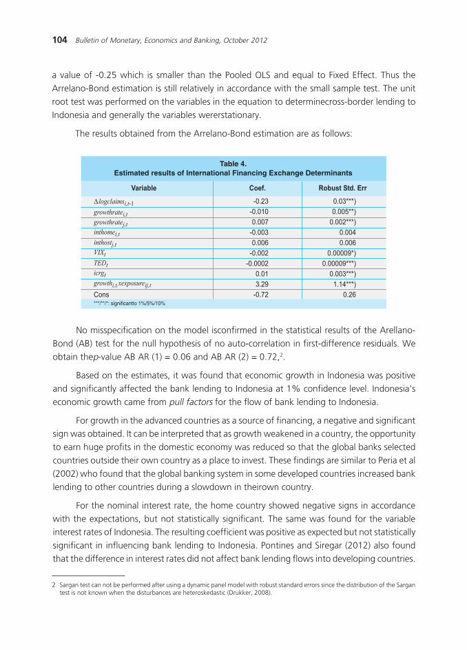
104 Bulletin of Monetary, Economics and Banking, October 2012
a value of -0.25 which is smaller than the Pooled OLS and equal to Fixed Effect. Thus the
Arrelano-Bond estimation is still relatively in accordance with the small sample test. The unit
root test was performed on the variables in the equation to determinecross-border lending to
Indonesia and generally the variables wererstationary.
The results obtained from the Arrelano-Bond estimation are as follows:
No misspecification on the model isconfirmed in the statistical results of the Arellano-
Bond (AB) test for the null hypothesis of no auto-correlation in first-difference residuals. We
obtain thep-value AB AR (1) = 0.06 and AB AR (2) = 0.72,2.
Based on the estimates, it was found that economic growth in Indonesia was positive
and significantly affected the bank lending to Indonesia at 1% confidence level. Indonesia’s
economic growth came from pull factors for the flow of bank lending to Indonesia.
For growth in the advanced countries as a source of financing, a negative and significantsign was obtained. It can be interpreted that as growth weakened in a country, the opportunity
to earn huge profits in the domestic economy was reduced so that the global banks selected
countries outside their own country as a place to invest. These findings are similar to Peria et al
(2002) who found that the global banking system in some developed countries increased bank
lending to other countries during a slowdown in theirown country.
For the nominal interest rate, the home country showed negative signs in accordance
with the expectations, but not statistically significant. The same was found for the variableinterest rates of Indonesia. The resulting coefficient was positive as expected but not statistically
significant in influencing bank lending to Indonesia. Pontines and Siregar (2012) also found
that the difference in interest rates did not affect bank lending flows into developing countries.
��� �� ���,- �� ������-�#��
2�0�: �0�:DDD�2�0�@� �0��EDD��0��F �0���DDD�2�0��: �0����0��G �0��G2�0��� �0����CD�2�0���� �0����CDDD��0�@ �0��:DDD�:0�C @0@�DDD�2�0F� �0�G
������������������ ����������� ��������
������������������������ ����������������
����
���������
����������������� �����������
������#$���%����������������&�������������!���� ����$' �����������%������
2 Sargan test can not be performed after using a dynamic panel model with robust standard errors since the distribution of the Sargantest is not known when the disturbances are heteroskedastic (Drukker, 2008).
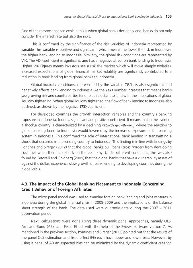
105Impact of Global Financial Shock to International Bank Lending in Indonesia
One of the reasons that can explain this is when global banks decide to lend, banks do not only
consider the interest rate but also the risks.
This is confirmed by the significance of the risk variables of Indonesia represented by
variable This variable is positive and significant, which means the lower the risk in Indonesia,
the higher bank lending to Indonesia. Similarly, the global risk conditions are represented by
VIX. The VIX coefficient is significant, and has a negative affect on bank lending to Indonesia.
Higher VIX Figures means investors see a risk the market which will move sharply (volatile).Increased expectations of global financial market volatility are significantly contributed to a
reduction in bank lending from global banks to Indonesia.
Global liquidity conditions, represented by the variable TEDt, is also significant and
negatively affects bank lending to Indonesia. As the TEDt number increases that means banks
see growing risk and counterparties tend to be reluctant to lend with the implications of global
liquidity tightening. When global liquidity tightened, the flow of bank lending to Indonesia alsodeclined, as shown by the negative TEDt coefficient.
For developed countries the growth interaction variables and the country’s banking
exposure in Indonesia, found a significant and positive coefficient. It means that in the event of
a shock,a country is characterized by a declining growth growthratei,t, where the reaction to
global banking loans to Indonesia would lowered by the increased exposure of the banking
system in Indonesia. This confirmed the role of international bank lending in transmitting ashock that occurred in the lending country to Indonesia. This finding is in line with findings by
Pontines and Siregar (2012) that the global banks pull loans (cross border) from developing
countries when there is a shock on the economy. Under different conditions, this was also
found by Cetorelli and Goldberg (2009) that the global banks that have a vulnerability assets of
against the dollar, experience slow growth of bank lending to developing countries during the
global crisis.
4.3. The Impact of the Global Banking Placement to Indonesia ConcerningCredit Behavior of Foreign Affiliates
The micro panel model was used to examine foreign bank lending and joint ventures in
Indonesia during the global financial crisis in 2008-2009 and the implications of the balance
sheet strength of the bank. The data used were quarterly data during the 2007 – 2011observation period.
Next, calculations were done using three dynamic panel approaches, namely OLS,
Arrelano-Bond (AB), and Fixed Effect with the help of the Eviews software version 7. As
mentioned in the previous section, Pontines and Siregar (2012) pointed out that the results of
the panel OLS estimation and fixed effect (FE) each have upper and lower bias. However, by
using a panel of AB an expected bias can be minimized by the dynamic coefficient criterion

106 Bulletin of Monetary, Economics and Banking, October 2012
variable of the model AB between the value of the coefficient of FE and OLS models. Based on
the parameter coefficient estimates, the value of the coefficient of dynamic variables logloani,t-
1 for FE models, AB, and OLS are 0651; 0655, and 0782, respectively. Thus, the estimated
value of the AB model is an eligible small sample.
��� �� ��#���$�.(�$��/�#�01
�0GEE��0�@:�DDD
�0��E��0�E@�DDD
2�0�@��0��C��0�G�
��0�AC�DDD�0�AF
��0��F�DDD�0�@
��0��G�D�0EFC
��0����DDD2�0�@
��0��@�DDD2�0@�:
��0�@A�DDD�0��F
��0��E�D�0�A
����������������� �����������
�����������
����������� �
������������ �
������� � �
���������� � �
!�"��
����#���
�����������������
����$ �����
����$ �����%����$ �������$�
���������
������(�)��%� �*����� ��������+�������������!�����������������,��--./�-��
Furthermore, the Sargan test was conducted to test whether the instruments wereexogenous. Where Ho is the overidentifying restriction (model specification) is valid. With a p-
valueof Sargan test = 0.48, the hypothesis Ho was accepted meaning the overidentifying
restriction (model specification) is valid.
Based on the above estimates of A-B models the effect of the economic conditions both
in the home country and the host country (domestic) on loans by foreign and joint venture
banks can be seen. The economic condition of the GDP and the interest rate of the host
country (Indonesia) wasa pull factor for lending by foreign banks / joint ventures. Economicconditions as reflected in economic growth and interest rates as a reflection of yields in Indonesia
showed a significant and positive sign. The positive sign of the GDP and the variable interest
rate in Indonesia was in accordance with the expected direction. On the other hand, economic
conditions (economic growth) of the home country (country of origin of foreign banks) also
showed a significant positive sign. This was a push factor for foreign affiliate banks to extend

107Impact of Global Financial Shock to International Bank Lending in Indonesia
credit in the host country (domestic). When economic growth in the country increases, foreign
banks tend to expand lending (international lending) to other countries, including Indonesia.
Meanwhile, the variable interest rate of the home country (country of origin of foreign banks)
showed a negative sign but was not significant.
The bank balance sheet variable NIM, also empirically demonstrated a positive direction
so that when foreign banks enjoyed a net interest margin that was higher, was a driver for the
foreign banks to extend credit. Meanwhile, the size of the bank was positive and significantmeaning the bigger foreign bank affiliate assets, the more they tended to add lending. There
was a positive and significant influence of the NIM and its size, in line with the findings by
Pontines (2012) using panel data of five ASEAN countries plus Korea. In the choosing portfolio
optimization for the placement of bank assets, ownership variables in the interbank money
market securities or in the equity markets were significant and negative. This means that the
credit and the placement on securities are substitutes.
Furthermore, the dummy crisis variable 2008/2009 was significant and negative. These
findings indicate that during the global financial crisis period, the loans granted by foreign
banks and joint venture banks tended to contract. This is also consistent with the findings of
Pontines and Siregar (2012) and Cetorelli and Goldberg (2009) who found that the credit
contraction also occurred in lending activities conducted by foreign affiliates in developing
countries during the global crisis.
However, when testing the stability of the foreign affiliate credit between the bank and
the bank branch of a foreign bank subsidiary, the interaction with the crisis dummy variable,
resulted in apositive and significant coefficient. These findings suggested that the bank subsidiary
has a more “crisis-mitigating impact” on the economy of Indonesia (host), especially when the
source of the shock comes from the global bank’s financial condition (parent) than foreign
banks. Factors that may explain this wasthe fixed cost that was irreversible and high whichinfluencedthe foreign direct investment banks to set up branches in the host country. This
made it difficultfor international banks “cut and run” during a crisis, both in the host country
and in the home country.
V. CONCLUSION
This paper provides some conclusions; first, as the monetary and banking system, Bank
Indonesia needs to understand the determinants of international bank lending to investigatethe impact of capital flows for the stability of the financial sector in Indonesia. This is because
exposure to financing from developed countries can be a transmission path forshock during a
financial turmoil in developed countries as a source of financing. Failure to understand the
relationship between the bank (global and regional) will pose a risk to the consistency of
macroeconomic policy formulation and the ability to anticipate the impact of the weakness of

108 Bulletin of Monetary, Economics and Banking, October 2012
the financial sector to the country’s macroeconomic conditions. Secondly, based on examination
of the determinants of financing to Indonesia, international factors exhibited significant affect
to bank lending as pull factors and push factors such as economic growth in the country of
origin and Indonesia. Risk factors for Indonesia and the global financial markets and global
liquidity conditions also exhibited significant affectsto bank lending to Indonesia. In addition,
the study also found that when there was a shock in a country, global banking would tend todecrease bank lending to Indonesia despite increased financing exposure in Indonesia. This
means that the bank lending directly (cross-border) transmits the shock from developed countries
to Indonesia. Third, based on the examination of bank lending and a mix of foreign banks in
Indonesia (foreign affiliates), it can be concluded that the activity of credit by foreign affiliates
are affected by domestic economic growth (pull factor) and the country of origin (push factor).
In the event of a crisis in the country of the parent bank, loans by foreign affiliates appeared tocontract. This means that the bank lending indirectly transmits shock from developed countries
to Indonesia. However, it is known that the estimation of foreign affiliates in the form of
subsidiary (locally incorparated) appeared more resistant to the shock of the financial turmoil
that occurred in the (home) country compared with the parent bank in the form of a branch
office.
These conclusions have policy implications both directly and indirectly. Empirically,
international bank lending is one shock transmission path from developed countries to Indonesiaeither directly (cross-border) and indirectly through the activities of foreign affiliates in Indonesia
credit. When there is a shock in the home country (parent bank), banks in developed countries
reduced bank lending activity in Indonesia. However, we found for foreign affiliates, subsidiary
bank credit activity (venture banks) appeared more stable than foreign banks. When there was
a crisis in their home country, the bank continued to see a mixture of credit activity comparedto foreign banks. Thereby supporting the subsidiary form of foreign banks may be one policy
option to support financial stability in Indonesia. However, encouraging foreign banking
subsidiaries does not mean a guarantee of complete isolation of the domestic banking system
from the possible sudden reversal of international bank lending. The role of regulators and
supervision remains an important factor in maintaining the stability of the banking sector as a
whole.

109Impact of Global Financial Shock to International Bank Lending in Indonesia
REFERENCES
Abdullah, Piter (2010). Foreign Claims by Global Banks: The Role and Implications In Indonesia.
Centre of Education & Central Bank Studies, Bank Indonesia.
Agenor, Pierre-Richard (1998). “The Surge in Capital Flows: Analysis of ‘Pull’ and ‘Push’ Factors”.
International Journal of Finance and Economics 3: 39–57.
Aiyar, Shekhar (2011), “How did the Crisis in International Funding Markets Affect Bank Lending?
Balance Sheet Evidence from the United Kingdom”, Bank of England, Working Paper No.424.
Allen, Frankliln, AnetaHryckiewicz, Oskar Kowalewski, and Günseli Tümer-Alkan (2012),
“Transmission of Bank Liquidity Shocks in Loan and Deposit Markets: The Role of Interbank
Borrowing and Market Monitoring”, Wharton Financial Institutions Center, Working Paper
10-28.
Calvo, Sara, and Carmen Reinhart, 1996, “Capital Flows to Latin America: Is There Evidence of
Contagion Effects?” in Private Capital Flows to Emerging Markets, ed. by G. Calvo andothers (Washington: Institute for International Economics).
Cetorelli, Nicola and Linda S. Goldberg (2010), “Global Banks and International Shock
Transmission: Evidence from the Crisis”, NBER Working Paper Series, Working Paper 15974.
Drukker, David M. (2008), “Summer North American Stata Users Group meeting”, Stata Corp.
1 / 32
Elton, Edwin J., Martin J. Gruber, Stephen J. Brown, and William N. Goetzmann (2003. Modern
Portfolio Theory and Investment Analysis, 6th ed. New Jersey: John Wiley and Sons Ltd.
Mian, Atif and AsimIjaz Khwaja (2006), “Tracing the Impact of Bank Liquidity Shocks: Evidencefrom an Emerging Market”, NBER Working Paper Series, Working Paper 12612.
Pontines, Victor and Reza Siregar (2012), “How Should We Bank With Foreigners? An Empirical
Assessment of Lending Behaviour of International Banks To Six East Asian Countries”, Centre
For Applied Macroeconomic Analysis, Working Paper 4.
Powell, Andrew, Maria Soledad Martinez Peria and IvannaVladkova (2002), “Banking on
Foreigners: The Behaviour of International Bank Lending to Latin America, 1985-2000”,
Centro de Invetigacion en Finanzas.

110 Bulletin of Monetary, Economics and Banking, October 2012
Siregar, Reza Y. (2012), “Globalized and Interconnected Banking System: Selected Issues and
Challenges”, AMRO.
Siregar, R.Y. and Choy K.M (2010), “Determinants of International Bank Lending from Developed
World to East Asia”, IMF Staff Papers, Vol. 57, No. 2, pp. 484-516.
Vita, Glauco De and KS Kyaw (2007). “Determinants of Capital Flows to Developing Countries:
A Structural VAR Analysis,” Journal of Economic Studies, Vol. 35 No. 4. 2008, pp. 304-322.
Zulverdi, Doddy, Iman Gunadi, Bambang Pramono, dan Wahyu Ari Wibowo (2004),
“Pengembangan Model Portofolio Bank”, Working Paper DKM BI.

111
WRITING GUIDANCE
1. The paper should be original and should not violate any copyrights. The submitted paper
should have never been published or not being submitted to other publisher. The copyright
of the published paper is retained to the author.
2. The Bulletin of Monetary Economics and Banking provide a financial incentive between IDR
1,000,000 to IDR 3,000,000.
3. The paper should be submitted in two formats (i) Microsoft Word (*.doc) and (ii) portable
digital file (*.PDF). These files should be sent to the following mail address:
[email protected] and Cc to: [email protected]
You may save your files in CD and send it to the following Editorial Address:
BULLETIN OF MONETARY ECONOMICS AND BANKING
Department of Economic Research and Monetary Policy-Bank Indonesia
Building Syafruddin Prawiranegara, 20th Floor
JI. M. H. Thamrin No.2 Central Jakarta, Indonesia
Ph. +62-21-2310108 / 2310408 ext. 4119, Fax: 62-21-3800394
4. To avoid missing fonts or other compatibility issues, any special characters or mathematical
expression (equations, symbols, matrix, etc.) must be written using Microsoft Equation.
5. The submitted paper should contain (i) an abstract of maximum one page A4, (ii) keywords
and (iii) JEL classification code. See the JEL code at http://www.aeaweb.org/journal/
jel_class_system.html.
6. The paper must contain the followings:
The background, the aim of the paper and its distinction to previous study
Theory and review of literatures
Methodology (quantitative methodology is preferred)
Result and analysis
Policy and further study implication
7. The citation should be in footnote and not in endnote.
8. The references must obey the following rule:

112 Bulletin of Monetary Economics and Banking, October 2010
a. Book:
HankeHankeHankeHankeHanke John E. John E. John E. John E. John E. and Arthur G. ReitschArthur G. ReitschArthur G. ReitschArthur G. ReitschArthur G. Reitsch, (1940), Business Forecasting, Prentice-Hall, New
Jersey.
b. Article in journal:
Rangazas, PeterRangazas, PeterRangazas, PeterRangazas, PeterRangazas, Peter. (2000) “Schooling and Economic Growth: A King-Rebelo Experiment
with Human Capital”, Journal of Monetary Economics, October , 46(2), page. 397-416.
c. Article in book edited by other people:
Frankel, Jeffrey AFrankel, Jeffrey AFrankel, Jeffrey AFrankel, Jeffrey AFrankel, Jeffrey A. and Andrew K., RoseAndrew K., RoseAndrew K., RoseAndrew K., RoseAndrew K., Rose. (1995) “Empirical Research on Nominal
Exchange Rates”, in Gene Grossman and Kenneth Rogoff, eds.,”Handbook of
International Economics. Amsterdam: North-Holland, page. 397-416.
d. Working papers:
Kremer, MichaelKremer, MichaelKremer, MichaelKremer, MichaelKremer, Michael and Daniel, ChenDaniel, ChenDaniel, ChenDaniel, ChenDaniel, Chen. (2000) “Income Distribution Dynamics with
Endogenous Fertility”. National Bureau of Economic Research (Cambridge, MA) Working
Paper No.7530.
e. Mimeo or unpublished work:
Knowles, JohnKnowles, JohnKnowles, JohnKnowles, JohnKnowles, John. “Can Parental Decision Explain U.S. Income Inequality?”, Mimeo,
University of Pennsylvania, 1999.
f. Article from web or other electronic form:
Summers, RobertSummers, RobertSummers, RobertSummers, RobertSummers, Robert and Alan WAlan WAlan WAlan WAlan W., Heston. Heston. Heston. Heston. Heston. (1997) “Penn World Table, Version 5.6”
http://pwt.econ.unpenn.edu/
g. Article in newspaper, magazine or equal periodicals:
Begley, SharonBegley, SharonBegley, SharonBegley, SharonBegley, Sharon. (1993) “Killed by Kindness”, Newsweek, April 12, page. 50-56.
9. The paper should be submitted along with curriculum vitae complete with mail address and
phone number.