Bulla et al 2016 Unexpected diversity in socially ... · 1 Unexpected diversity in socially synchronized rhythms of shorebirds . Martin Bulla. 1, Mihai Valcu. 1, Adriaan M. Dokter

1

Unexpected diversity in socially synchronized rhythms of shorebirds

Martin Bulla1, Mihai Valcu

1, Adriaan M. Dokter

2, Alexei G. Dondua

3, András Kosztolányi

4,5, Anne Rutten

1,6, Barbara Helm

7, Brett K.

Sandercock8, Bruce Casler

9, Bruno J. Ens

10, Caleb S. Spiegel

11, Chris J. Hassell

12, Clemens Küpper

13, Clive Minton

14, Daniel Burgas

15,16,

David B. Lank17

, David C. Payer18

, Egor Y. Loktionov19

, Erica Nol20

, Eunbi Kwon21

, Fletcher Smith22

, H. River Gates23

, Hana Vitnerová24

,

Hanna Prüter25

, James A. Johnson26

, James J. H. St Clair27,28

, Jean-François Lamarre29

, Jennie Rausch30

, Jeroen Reneerkens31

, Jesse R.

Conklin31

, Joanna Burger32

, Joe Liebezeit33

, Joël Bêty29

, Jonathan T. Coleman34

, Jordi Figuerola35

, Jos C. E. W. Hooijmeijer31

, José A.

Alves36,37

, Joseph A. M. Smith38

, Karel Weidinger39

, Kari Koivula40

, Ken Gosbell41

, Larry Niles42

, Laura Koloski43

, Laura McKinnon44

, Libor

Praus39

, Marcel Klaassen45

, Marie-Andrée Giroux46,47

, Martin Sládeček48

, Megan L. Boldenow49

, Michael Exo50

, Michael I. Goldstein51

,

Miroslav Šálek48

, Nathan Senner31,52

, Nelli Rönkä40

, Nicolas Lecomte47

, Olivier Gilg53,54

, Orsolya Vincze55,56

, Oscar W. Johnson57

, Paul A.

Smith58

, Paul F. Woodard30

, Pavel S. Tomkovich59

, Phil Battley60

, Rebecca Bentzen61

, Richard B. Lanctot26

, Ron Porter62

, Sarah T.

Saalfeld26

, Scott Freeman63

, Stephen C. Brown64

, Stephen Yezerinac65

, Tamás Székely66

, Tomás Montalvo67

, Theunis Piersma31,68

,

Vanessa Loverti69

, Veli-Matti Pakanen40

, Wim Tijsen70

, Bart Kempenaers1

1Department of Behavioural Ecology and Evolutionary Genetics, Max Planck Institute for Ornithology, Eberhard Gwinner Str, 82319 Seewiesen, Germany. 2Computational

Geo-Ecology, Institute for Biodiversity and Ecosystem Dynamics, University of Amsterdam, Science Park 904, 1098 XH, Amsterdam, The Netherlands. 3Independent

researcher, Gatchinskaya, ap. 27, 197198, St-Petersburg, Russia. 4Department of Ecology, University of Veterinary Medicine Budapest, Rottenbiller u. 50., H-1077, Budapest,

Hungary. 5MTA-DE "Lendület" Behavioural Ecology Research Group, Department of Evolutionary Zoology, University of Debrecen, Egyetem tér 1., H-4032, Debrecen, Hungary. 6Apiloa GmbH, 82319, Starnberg, Germany. 7Institute of Biodiversity Animal Health and Comparative Medicine, University of Glasgow, Graham Kerr Building, G12 8QQ,

Glasgow, UK. 8Division of Biology, Kansas State University, 116 Ackert Hall, 66506-4901, Manhattan, KS, USA. 9PO Box 1094, 89407, Fallon, NV, USA. 10Coastal Ecology Team,

Sovon Dutch Centre for Field Ornithology, PO box 59, 1790 AB, Den Burg, Texel, The Netherlands. 11Division of Migratory Birds, Northeast Region, US Fish & Wildlife Service,

300 Westgate Center Dr, 01035, Hadley, MA, USA. 12Global Flyway Network, PO Box 3089, WA 6725, Broome, Australia. 13Institute of Zoology, University of Graz,

Universitätsplatz 2, 8010, Graz, Austria. 14Victorian Wader Study group, 165 Dalgetty Road, 3193, Beaumaris, Australia. 15Department of Forest Sciences, University of Helsinki,

PO Box 27, FI-00014, Helsinki, Finland. 16Department of Biological and Environmental Sciences, University of Jyväskylä, PO Box 35, FI-40014, Jyväskylä, Finland. 17Department

of Biological Sciences, Simon Fraser University, 8888 University Drive, V5A 1S6, Burnaby, BC, Canada. 18Alaska Region, U.S. National Park Service, 240 W. 5th Ave, 99501,

Anchorage, AK, USA. 19State Lab for Photon Energetics, Bauman Moscow State Technical University, 2nd Baumanskaya St., 5-1, 105005, Moscow, Russia. 20Biology

Department, Trent University, 2140 East Bank Drive, K9L 0G2, Peterborough, ON, Canada. 21Department of Fish and Wildlife Conservation, Virginia Polytechnic Institute and

State University, 310 West Campus Drive, 24061, Blacksburg, VA, USA. 22Center for Conservation Biology, College of William & Mary and Virginia Commonwealth University,

PO Box 8795, 23187, Williamsburg, Virginia, USA. 23ABR, Inc. Environmental Research and Services, PO Box 240268, 99524, Anchorage, AK, USA. 24Faculty of Science, Charles

University in Prague, Albertov 6, 128 43, Praha 2, Czech Republic. 25Department of Wildlife Diseases, Leibniz Institute for Zoo- and Wildlife Research, Alfred-Kowalke-Straße

17, 10315, Berlin, Germany. 26Migratory Bird Management, US Fish and Wildlife Service, 1011 East Tudor Road, 99503, Anchorage, USA. 27Biodiversity Lab, Department of

Biology and Biochemistry, University of Bath, Claverton Down, BA1 7AY, Bath, UK. 28Centre for Evolutionary Biology, University of Western Australia, Stirling Highway, WA

6009, Crawley, Australia. 29Biologie, Chimie et Géographie, Université du Québec à Rimouski , 300, allée des Ursulines, G5L 3A8, Rimouski. QC, Canada. 30Canadian Wildlife

Service, Environment and Climate Change Canada, P.O. Box 2310, 5019 – 52nd Street, 4th Floor, X1A2P7, Yellowknife NT, Canada. 31Conservation Ecology Group, Groningen

Institute for Evolutionary Life Sciences, University of Groningen, Nijenborgh 7, 9747 AG, Groningen, The Netherlands. 32Division of Life Sciences, Rutgers University, 604‑

Allison Road, NJ 08854‑8082, Piscataway, USA. 33Audubon Society of Portland, 5151 NW Cornell Road, 97210, Portland, OR, USA. 34Queensland Wader Study Group, 22 Parker

Street, 4128, Queensland, Australia. 35Department of Wetland Ecology, Doñana Biological Station (CSIC), Av. Americo Vespucio, s/n., 41092, Seville, Spain. 36Centre for

Environmental and Marine Studies (CESAM), Dep. Biology, University of Aveiro, Campus de Santiago, 3810-193, Aveiro, Portugal. 37South Iceland Research Centre, University

of Iceland, Fjolheimar, 800, Selfoss, Iceland. 38Conservation Services International, PO Box 784, 8204, Cape May, NJ, USA. 39Department of Zoology and Laboratory of

Ornithology, Palacký University, 17. listopadu 50, 771 46, Olomouc, Czech Republic. 40Department of Ecology, University of Oulu, PO Box 3000, 90014, Oulu, Finland. 41Australasian Wader Studies Group, 1/19 Baldwin Road, 3130, Blackburn, Australia. 42LJ Niles Associates, 109 market lane, 8323, Greenwich, USA. 43Environmental and Life

Sciences, Trent University, 1600 West Bank Dr., K0L 0G2, Peterborough, ON, Canada. 44Bilingual Biology Program, York University Glendon Campus, 2275 Bayview Avenue,

M4N 3M6, Toronto, ON, Canada. 45Centre for Integrative Ecology, Deakin University, 75 Pigdons Road, VIC 3216, Waurn Ponds, Australia. 46Canada Research in Northern

Biodiversity and Centre d'Études Nordiques, Université du Québec à Rimouski, 300, allée des Ursulines, G5L 3A8 , Rimouski, QC, Canada. 47

Canada Research in Polar and

Boreal Ecology and Centre d'Études Nordiques, Université de Moncton, 18 avenue Antonine-Maillet, E4K 1A6, Moncton, NB, Canada. 48

Faculty of Environmental Sciences,

Czech University of Life Sciences Prague, Kamýcká 1176, Suchdol, 16521, Prague, Czech Republic. 49Depatment of Biology and Wildlife, University of Alaska Fairbanks, PO Box

756100, 99775-6100, Fairbanks, AK, USA. 50Vogelwarte Helgoland, Institut für Vogelforschung, An der Vogelwarte 21, D-26386, Wilhelmshaven, Germany. 51Alaska Coastal

Rainforest Center, University of Alaska Southeast, 11120 Glacier Hwy, 99801, Juneau, AK, USA. 52

Cornell Lab of Ornithology, 159 Sapsucker Woods Road, 14850, Ithaca, USA. 53

Equipe Ecologie-Evolution, UMR 6282 Biogéosciences, Université de Bourgogne, 6 Bd Gabriel, 21000, Dijon, France. 54

Groupe de Recherche en Ecologie Arctique, 16 rue de

Vernot, 21440, Francheville, France. 55

Department of Evolutionary Zoology and Human Biology, University of Debrecen, Egyetem tér 1., H-4032, Debrecen, Hungary. 56Hungarian Department of Biology and Ecology, Babeş-Bolyai University, Clinicilor 5-7, RO-400006, Cluj-Napoca, Romania. 57Department of Ecology, Montana State

University, MT 59717, Bozeman, USA. 58Wildlife Research Division, Environment and Climate Change Canada, 1125 Colonel By Dr., K1A 0H3, Ottawa, ON, Canada. 59Zoological

Museum, Lomonosov Moscow State University, Bolshaya Nikitskaya St., 6, 125009, Moscow, Russia. 60Institute of Agriculture & Environment, Massey University, Private Bag

11 222, 4442, Palmerston north, New Zealand. 61

Arctic Beringia Program, Wildlife Conservation Society, 925 Schloesser Dr., 99709, Fairbanks, AK, USA. 62

Delaware Bay

Shorebird Project, 19002, Ambler, PA, USA. 63Arctic National Wildlife Refuge, US Fish & Wildlife Service, 101 12th Ave, 99701, Fairbanks, AK, USA. 64Shorebird Recovery

Program, Manomet, PO Box 545, 05154, Saxtons River, VT, USA. 65Fieldday Consulting, V4N 6M5, Surrey, BC, Canada. 66Milner Centre for Evolution, Department of Biology

and Biochemistry, University of Bath, Claverton Down, BA2 7AY, Bath, UK. 67Servei de Vigilància i Control de Plagues Urbanes, Agència de Salut Pública de Barcelona, Av.

Príncep d’Astúries 63, 8012, Barcelona, Spain. 68

Department of Marine Ecology, NIOZ Royal Netherlands Institute for Sea Research, PO Box 59, 1790AB, Den Burg, Texel, The

Netherlands. 69

Migratory Bird and Habitat Program, U.S. Fish and Wildlife Service, 911 NE 11th Avenue, 97232, Portland, OR, USA. 70

Poelweg 12, 1778 KB, Westerland, The

Netherlands.

. CC-BY-NC-ND 4.0 International licensenot peer-reviewed) is the author/funder. It is made available under aThe copyright holder for this preprint (which was. http://dx.doi.org/10.1101/084806doi: bioRxiv preprint first posted online Nov. 1, 2016;

http://dx.doi.org/10.1101/084806

http://creativecommons.org/licenses/by-nc-nd/4.0/

2

The behavioural rhythms of organisms are thought to be under strong selection, influenced by the

rhythmicity of the environment1-4. Behavioural rhythms are well studied in isolated individuals under

laboratory conditions1,5, but in free-living populations, individuals have to temporally synchronize their

activities with those of others, including potential mates, competitors, prey and predators6-10. Individuals

can temporally segregate their daily activities (e.g. prey avoiding predators, subordinates avoiding

dominants) or synchronize their activities (e.g. group foraging, communal defence, pairs reproducing or

caring for offspring)6-9,11. The behavioural rhythms that emerge from such social synchronization and the

underlying evolutionary and ecological drivers that shape them remain poorly understood5-7,9. Here, we

address this in the context of biparental care, a particularly sensitive phase of social synchronization12 where

pair members potentially compromise their individual rhythms. Using data from 729 nests of 91 populations

of 32 biparentally-incubating shorebird species, where parents synchronize to achieve continuous coverage

of developing eggs, we report remarkable within- and between-species diversity in incubation rhythms.

Between species, the median length of one parent’s incubation bout varied from one to 19 hours, while

period length – the cycle of female and male probability to incubate – varied from six to 43 hours. The

length of incubation bouts was unrelated to variables reflecting energetic demands, but species relying on

crypsis had longer incubation bouts than those that are readily visible or actively protect their nest against

predators. Rhythms entrainable to the 24-h light-dark cycle were less likely at high latitudes and absent in

18 species. Our results indicate that even under similar environmental conditions and despite 24-h

environmental cues, social synchronization can generate far more diverse behavioural rhythms than

expected from studies of individuals in captivity5-7,9. The risk of predation, not the risk of starvation, may be

a key factor underlying the diversity in these rhythms.

Incubation by both parents prevails in almost 80% of non-passerine families13 and is the most common form of

care in shorebirds14. Biparental shorebirds are typically monogamous15, mostly lay three or four eggs in an

open nest on the ground15, and cover their eggs almost continuously13. Pairs achieve this through

synchronization of their activities such that one of them is responsible for the nest at a given time (i.e. an

incubation bout). Alternating female and male bouts generate an incubation rhythm with a specific period

length (cycle of high and low probability for a parent to incubate).

We used diverse monitoring systems (Methods & Extended Data Table 1) to collect data on incubation

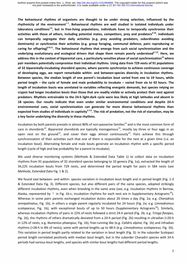
rhythms from 91 populations of 32 shorebird species belonging to 10 genera (Fig. 1a), extracted the length of

34,225 incubation bouts from 729 nests, and determined the period length for pairs in 584 nests (see

Methods, Extended Data Fig. 1 & 2).

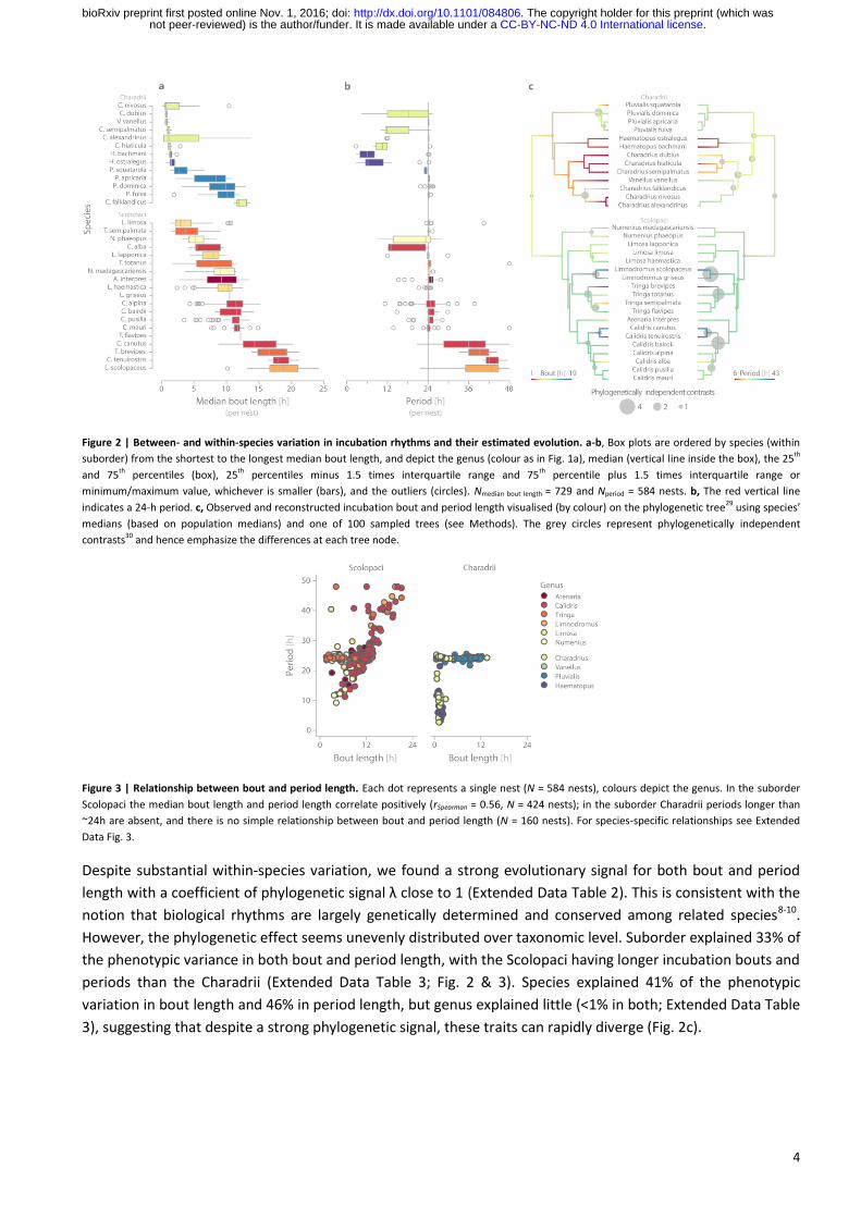
We found vast between- and within- species variation in incubation bout length and in period length (Fig. 1-3

& Extended Data Fig. 3). Different species, but also different pairs of the same species, adopted strikingly

different incubation rhythms, even when breeding in the same area (see, e.g. incubation rhythms in Barrow,

Alaska, represented by in Fig. 1b-c; incubation rhythms for each nest are in Supplementary Actograms16).

Whereas in some pairs parents exchanged incubation duties about 20 times a day (Fig. 2a; e.g. Charadrius

semipalmatus, Fig. 1b), in others a single parent regularly incubated for 24 hours (Fig. 2a; e.g. Limnodromus

scolopaceus, Fig. 1b), with exceptional bouts of up to 50 hours (Supplementary Actograms16). Similarly,

whereas incubation rhythms of pairs in 22% of nests followed a strict 24-h period (Fig. 2b; e.g. Tringa flavipes,

Fig. 1b), the rhythms of others dramatically deviated from a 24-h period (Fig. 2b) resulting in ultradian (<20-h

in 12% of nests; e.g. Numenius phaeopus; Fig. 1b), free-running like (e.g. Calidris alpina; Fig. 1b) and infradian

rhythms (>28-h in 8% of nests), some with period lengths up to 48-h (e.g. Limnodromus scolopaceus; Fig. 1b).

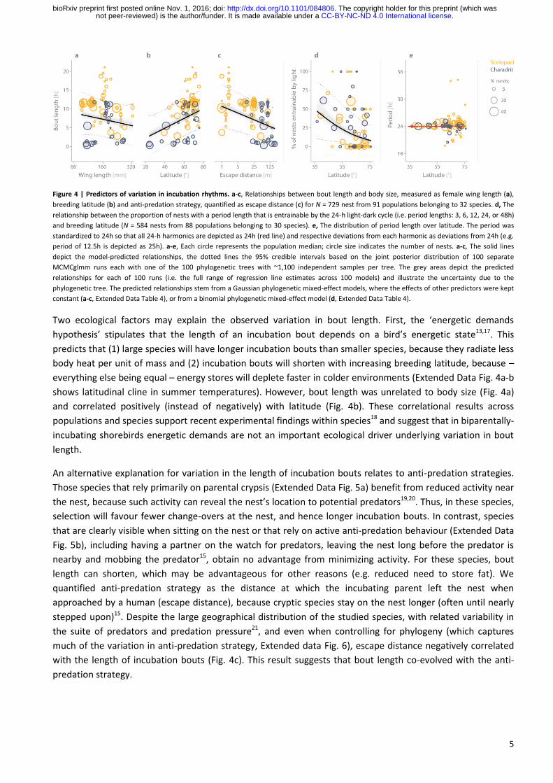
This variation in period length partly related to the variation in bout length (Fig. 3): in the suborder Scolopaci

period length correlated positively with median bout length, but in the suborder Charadrii species with 24-h

periods had various bout lengths, and species with similar bout lengths had different period lengths.


http://dx.doi.org/10.1101/084806


3

Figure 1 | Map of studied

breeding sites and the

diversity of shorebird

incubation rhythms. a, Map of

breeding sites with data on

incubation rhythms. The

colour of the dots indicates the

genus (data from multiple

species per genus may be

available), the size of the dots

refers to data quality ( ,

large: exact breeding site

known; , small: breeding site

estimated, see Methods). For

nearby or overlapping

locations, the dots are

scattered to increase visibility.

Contours of the map made

with Natural Earth,

http://www.naturalearthdata.

com. b-c, Illustrations of

between-species diversity (b)

and within-species diversity (c;

note that the three rhythms

for Western sandpiper and

Ringed plover come from the

same breeding location.). Each

actogram depicts the bouts of

female (yellow; ) and male

(blue-grey; ) incubation at a

single nest over a 24-h period,

plotted twice, such that each

row represents two

consecutive days. If present,

twilight is indicated by light

grey bars ( ) and

corresponds to the time when

the sun is between 6° and 0°

below the horizon, night is

indicated by dark grey bars (

) and corresponds to the

time when the sun is < 6°

below the horizon. Twilight

and night are omitted in the

centre of the actogram (24:00)

to make the incubation rhythm

visible. a, Between-species

diversity. a-c, The circled

numbers ( ) indicate

the breeding site of each pair

and correspond to the

numbers on the map.


http://www.naturalearthdata.com/

http://www.naturalearthdata.com/

http://dx.doi.org/10.1101/084806


4

Figure 2 | Between- and within-species variation in incubation rhythms and their estimated evolution. a-b, Box plots are ordered by species (within

suborder) from the shortest to the longest median bout length, and depict the genus (colour as in Fig. 1a), median (vertical line inside the box), the 25th

and 75th percentiles (box), 25th percentiles minus 1.5 times interquartile range and 75th percentile plus 1.5 times interquartile range or

minimum/maximum value, whichever is smaller (bars), and the outliers (circles). Nmedian bout length = 729 and Nperiod = 584 nests. b, The red vertical line

indicates a 24-h period. c, Observed and reconstructed incubation bout and period length visualised (by colour) on the phylogenetic tree29 using species’

medians (based on population medians) and one of 100 sampled trees (see Methods). The grey circles represent phylogenetically independent

contrasts30 and hence emphasize the differences at each tree node.

Figure 3 | Relationship between bout and period length. Each dot represents a single nest (N = 584 nests), colours depict the genus. In the suborder

Scolopaci the median bout length and period length correlate positively (rSpearman = 0.56, N = 424 nests); in the suborder Charadrii periods longer than

~24h are absent, and there is no simple relationship between bout and period length (N = 160 nests). For species-specific relationships see Extended

Data Fig. 3.

Despite substantial within-species variation, we found a strong evolutionary signal for both bout and period

length with a coefficient of phylogenetic signal λ close to 1 (Extended Data Table 2). This is consistent with the

notion that biological rhythms are largely genetically determined and conserved among related species8-10.

However, the phylogenetic effect seems unevenly distributed over taxonomic level. Suborder explained 33% of

the phenotypic variance in both bout and period length, with the Scolopaci having longer incubation bouts and

periods than the Charadrii (Extended Data Table 3; Fig. 2 & 3). Species explained 41% of the phenotypic

variation in bout length and 46% in period length, but genus explained little (<1% in both; Extended Data Table

3), suggesting that despite a strong phylogenetic signal, these traits can rapidly diverge (Fig. 2c).


http://dx.doi.org/10.1101/084806


5

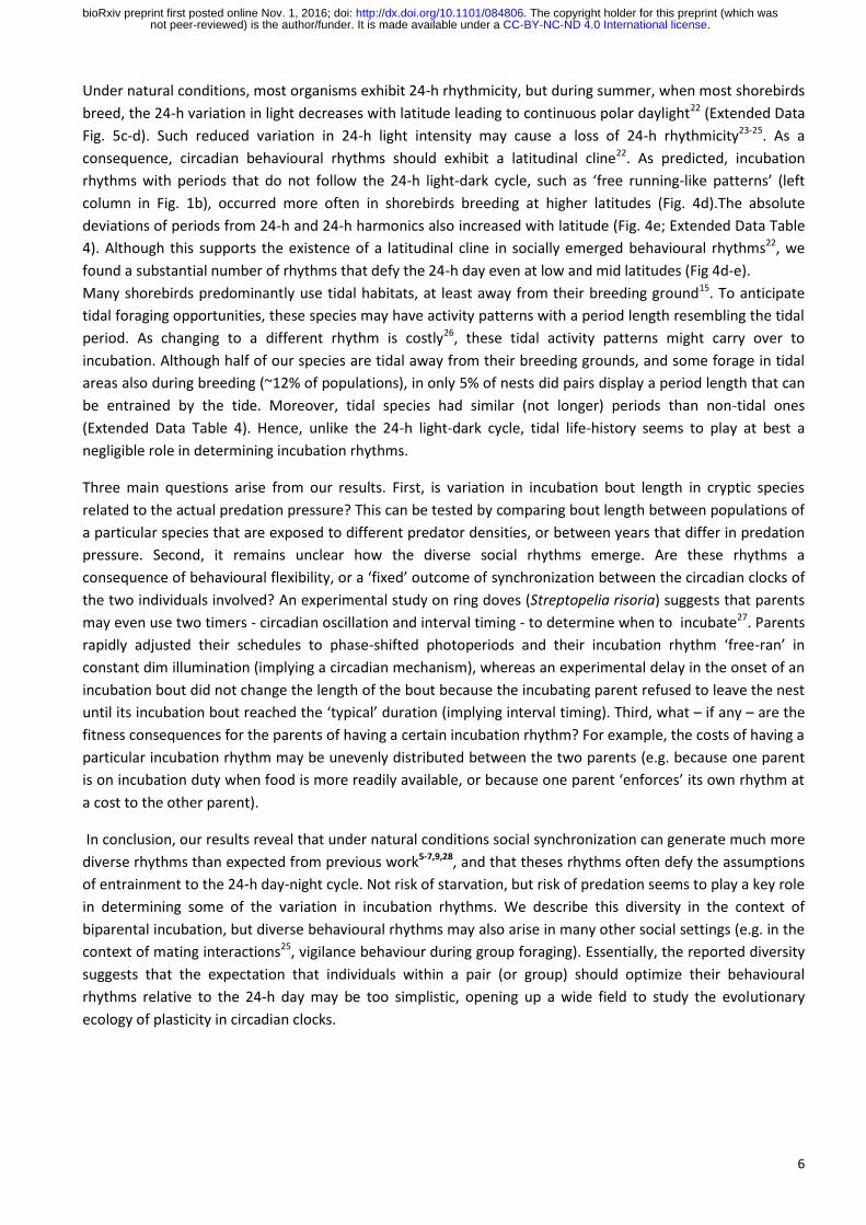
Figure 4 | Predictors of variation in incubation rhythms. a-c, Relationships between bout length and body size, measured as female wing length (a),

breeding latitude (b) and anti-predation strategy, quantified as escape distance (c) for N = 729 nest from 91 populations belonging to 32 species. d, The

relationship between the proportion of nests with a period length that is entrainable by the 24-h light-dark cycle (i.e. period lengths: 3, 6, 12, 24, or 48h)

and breeding latitude (N = 584 nests from 88 populations belonging to 30 species). e, The distribution of period length over latitude. The period was

standardized to 24h so that all 24-h harmonics are depicted as 24h (red line) and respective deviations from each harmonic as deviations from 24h (e.g.

period of 12.5h is depicted as 25h). a-e, Each circle represents the population median; circle size indicates the number of nests. a-c, The solid lines

depict the model-predicted relationships, the dotted lines the 95% credible intervals based on the joint posterior distribution of 100 separate

MCMCglmm runs each with one of the 100 phylogenetic trees with ~1,100 independent samples per tree. The grey areas depict the predicted

relationships for each of 100 runs (i.e. the full range of regression line estimates across 100 models) and illustrate the uncertainty due to the

phylogenetic tree. The predicted relationships stem from a Gaussian phylogenetic mixed-effect models, where the effects of other predictors were kept

constant (a-c, Extended Data Table 4), or from a binomial phylogenetic mixed-effect model (d, Extended Data Table 4).

Two ecological factors may explain the observed variation in bout length. First, the ‘energetic demands

hypothesis’ stipulates that the length of an incubation bout depends on a bird’s energetic state13,17. This

predicts that (1) large species will have longer incubation bouts than smaller species, because they radiate less

body heat per unit of mass and (2) incubation bouts will shorten with increasing breeding latitude, because –

everything else being equal – energy stores will deplete faster in colder environments (Extended Data Fig. 4a-b

shows latitudinal cline in summer temperatures). However, bout length was unrelated to body size (Fig. 4a)

and correlated positively (instead of negatively) with latitude (Fig. 4b). These correlational results across

populations and species support recent experimental findings within species18 and suggest that in biparentally-

incubating shorebirds energetic demands are not an important ecological driver underlying variation in bout

length.

An alternative explanation for variation in the length of incubation bouts relates to anti-predation strategies.

Those species that rely primarily on parental crypsis (Extended Data Fig. 5a) benefit from reduced activity near

the nest, because such activity can reveal the nest’s location to potential predators19,20. Thus, in these species,

selection will favour fewer change-overs at the nest, and hence longer incubation bouts. In contrast, species

that are clearly visible when sitting on the nest or that rely on active anti-predation behaviour (Extended Data

Fig. 5b), including having a partner on the watch for predators, leaving the nest long before the predator is

nearby and mobbing the predator15, obtain no advantage from minimizing activity. For these species, bout

length can shorten, which may be advantageous for other reasons (e.g. reduced need to store fat). We

quantified anti-predation strategy as the distance at which the incubating parent left the nest when

approached by a human (escape distance), because cryptic species stay on the nest longer (often until nearly

stepped upon)15. Despite the large geographical distribution of the studied species, with related variability in

the suite of predators and predation pressure21, and even when controlling for phylogeny (which captures

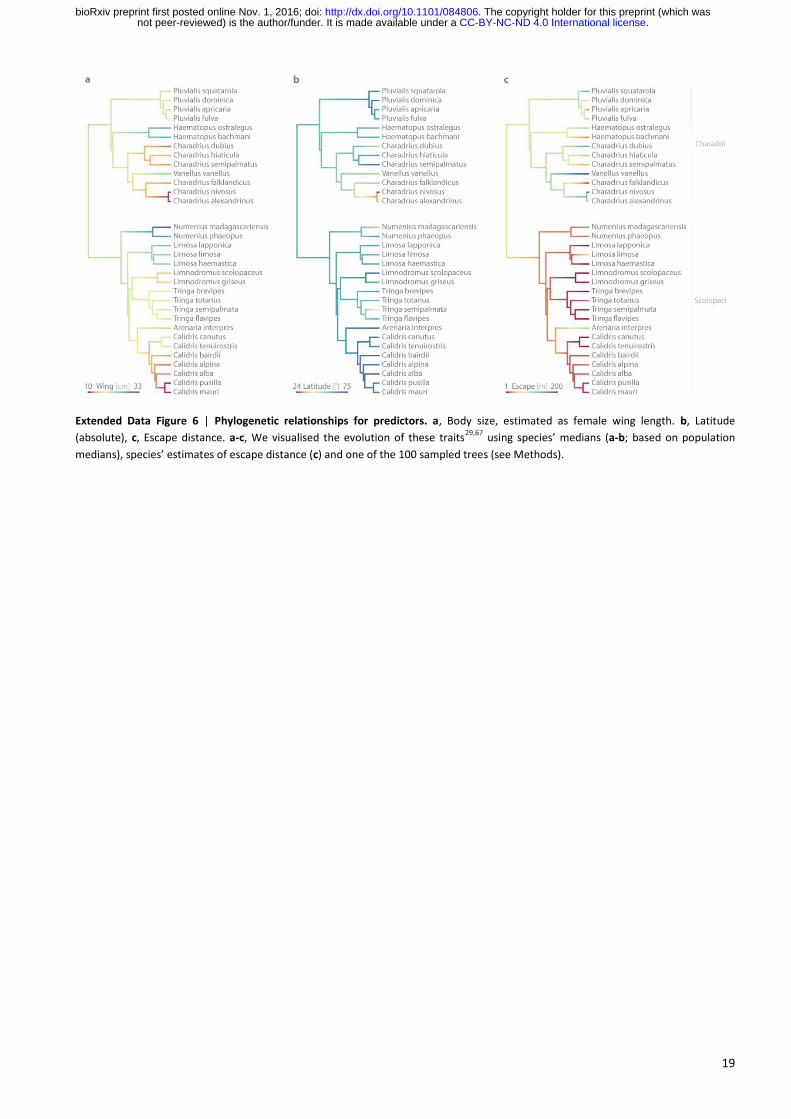
much of the variation in anti-predation strategy, Extended data Fig. 6), escape distance negatively correlated

with the length of incubation bouts (Fig. 4c). This result suggests that bout length co-evolved with the anti-

predation strategy.


http://dx.doi.org/10.1101/084806


6

Under natural conditions, most organisms exhibit 24-h rhythmicity, but during summer, when most shorebirds

breed, the 24-h variation in light decreases with latitude leading to continuous polar daylight22 (Extended Data

Fig. 5c-d). Such reduced variation in 24-h light intensity may cause a loss of 24-h rhythmicity23-25. As a

consequence, circadian behavioural rhythms should exhibit a latitudinal cline22. As predicted, incubation

rhythms with periods that do not follow the 24-h light-dark cycle, such as ‘free running-like patterns’ (left

column in Fig. 1b), occurred more often in shorebirds breeding at higher latitudes (Fig. 4d).The absolute

deviations of periods from 24-h and 24-h harmonics also increased with latitude (Fig. 4e; Extended Data Table

4). Although this supports the existence of a latitudinal cline in socially emerged behavioural rhythms22, we

found a substantial number of rhythms that defy the 24-h day even at low and mid latitudes (Fig 4d-e).

Many shorebirds predominantly use tidal habitats, at least away from their breeding ground15. To anticipate

tidal foraging opportunities, these species may have activity patterns with a period length resembling the tidal

period. As changing to a different rhythm is costly26, these tidal activity patterns might carry over to

incubation. Although half of our species are tidal away from their breeding grounds, and some forage in tidal

areas also during breeding (~12% of populations), in only 5% of nests did pairs display a period length that can

be entrained by the tide. Moreover, tidal species had similar (not longer) periods than non-tidal ones

(Extended Data Table 4). Hence, unlike the 24-h light-dark cycle, tidal life-history seems to play at best a

negligible role in determining incubation rhythms.

Three main questions arise from our results. First, is variation in incubation bout length in cryptic species

related to the actual predation pressure? This can be tested by comparing bout length between populations of

a particular species that are exposed to different predator densities, or between years that differ in predation

pressure. Second, it remains unclear how the diverse social rhythms emerge. Are these rhythms a

consequence of behavioural flexibility, or a ‘fixed’ outcome of synchronization between the circadian clocks of

the two individuals involved? An experimental study on ring doves (Streptopelia risoria) suggests that parents

may even use two timers - circadian oscillation and interval timing - to determine when to incubate27. Parents

rapidly adjusted their schedules to phase-shifted photoperiods and their incubation rhythm ‘free-ran’ in

constant dim illumination (implying a circadian mechanism), whereas an experimental delay in the onset of an

incubation bout did not change the length of the bout because the incubating parent refused to leave the nest

until its incubation bout reached the ‘typical’ duration (implying interval timing). Third, what – if any – are the

fitness consequences for the parents of having a certain incubation rhythm? For example, the costs of having a

particular incubation rhythm may be unevenly distributed between the two parents (e.g. because one parent

is on incubation duty when food is more readily available, or because one parent ‘enforces’ its own rhythm at

a cost to the other parent).

In conclusion, our results reveal that under natural conditions social synchronization can generate much more

diverse rhythms than expected from previous work5-7,9,28, and that theses rhythms often defy the assumptions

of entrainment to the 24-h day-night cycle. Not risk of starvation, but risk of predation seems to play a key role

in determining some of the variation in incubation rhythms. We describe this diversity in the context of

biparental incubation, but diverse behavioural rhythms may also arise in many other social settings (e.g. in the

context of mating interactions25, vigilance behaviour during group foraging). Essentially, the reported diversity

suggests that the expectation that individuals within a pair (or group) should optimize their behavioural

rhythms relative to the 24-h day may be too simplistic, opening up a wide field to study the evolutionary

ecology of plasticity in circadian clocks.


http://dx.doi.org/10.1101/084806


7

REFERENCES

1, Dunlap, J. C., Loros, J. J. & DeCoursey, P. J. Chronobiology: Biological Timekeeping (Sinauer Associates, 2004).

2, Young, M. W. & Kay, S. A. Time zones: a comparative genetics of circadian clocks. Nat Rev Genet 2, 702-715 (2001).

3, Helm, B. & Visser, M. E. Heritable circadian period length in a wild bird population. Proc R Soc B (2010).

4, Koskenvuo, M., Hublin, C., Partinen, M., Heikkilä, K. & Kaprio, J. Heritability of diurnal type: a nationwide study of 8753

adult twin pairs. J Sleep Res 16, 156-162 (2007).

5, Kronfeld-Schor, N., Bloch, G. & Schwartz, W. J. Animal clocks: when science meets nature. Proc R Soc B 280 (2013).

6, Bloch, G., Herzog, E. D., Levine, J. D. & Schwartz, W. J. Socially synchronized circadian oscillators. Proc R Soc B 280

(2013).

7, Castillo-Ruiz, A., Paul, M. J. & Schwartz, W. J. In search of a temporal niche: social interactions. Prog Brain Res 199, 267-

280 (2012).

8, Mistlberger, R. E. & Skene, D. J. Social influences on mammalian circadian rhythms: animal and human studies. Biol Rev

79, 533-556 (2004).

9, Davidson, A. J. & Menaker, M. Birds of a feather clock together–sometimes: social synchronization of circadian

rhythms. Curr Opin Neurobiol 13, 765-769 (2003).

10, Mrosovsky, N. Locomotor activity and non‐photic influences on circadian clocks. Biol Rev 71, 343-372 (1996).

11, Regal, P. J. & Connolly, M. S. Social influences on biological rhythms. Behaviour 72, 171-198 (1980).

12, Emlen, S. T. & Oring, L. W. Ecology, sexual selection, and the evolution of mating systems. Science 197, 215-223

(1977).

13, Deeming, D. C. Avian Incubation: Behaviour, Environment and Evolution (Oxford University Press, 2002).

14, Szekely, T. & Reynolds, J. D. Evolutionary transitions in parental care in shorebirds. Proc R Soc B 262, 57-64 (1995).

15, del Hoyo, J., Elliott, A. & Sargatal, J. Handbook of the Birds of the World. Vol. 3. Hoatzing to Auks. (Lynx Edicions,

1996).

16, Bulla, M. et al. Supporting Information for 'Unexpected diversity in socially synchronized rhythms of shorebirds'.

Version 1. Open Science Framework, https://osf.io/wxufm/ (2016).

17, Williams, J. B. in Avian Energetics and Nutritional Ecology (ed C. Carey) Ch. 5, 375-416 (Chapman & Hall, 1996).

18, Bulla, M., Cresswell, W., Rutten, A. L., Valcu, M. & Kempenaers, B. Biparental incubation-scheduling: no experimental

evidence for major energetic constraints. Behav Ecol 26, 30-37 (2015).

19, Martin, T. E., Scott, J. & Menge, C. Nest predation increases with parental activity: separating nest site and parental

activity effects. Proc R Soc B 267, 2287-2293 (2000).

20, Smith, P. A., Tulp, I., Schekkerman, H., Gilchrist, H. G. & Forbes, M. R. Shorebird incubation behaviour and its influence

on the risk of nest predation. Anim Behav 84, 835-842 (2012).

21, McKinnon, L. et al. Lower predation risk for migratory birds at high latitudes. Science 327, 326-327 (2010).

22, Hut, R. A., Paolucci, S., Dor, R., Kyriacou, C. P. & Daan, S. Latitudinal clines: an evolutionary view on biological rhythms.

Proc R Soc B 280, 20130433 (2013).

23, van Oort, B. E. et al. Circadian organization in reindeer. Nature 438, 1095-1096 (2005).

24, Steiger, S. S. et al. When the sun never sets: diverse activity rhythms under continuous daylight in free-living arctic-

breeding birds. Proc R Soc B 280 (2013).

25, Lesku, J. A. et al. Adaptive sleep loss in polygynous pectoral sandpipers. Science 337, 1654-1658 (2012).

26, Foster, R. G. & Wulff, K. The rhythm of rest and excess. Nat Rev Neurosci 6, 407-414 (2005).

27, Silver, R. & Bittman, E. L. Reproductive Mechanisms: Interaction of Circadian and Interval Timing. Ann N Y Acad Sci

423, 488-514 (1984).

28, Paul, M. J., Indic, P. & Schwartz, W. J. Social synchronization of circadian rhythmicity in female mice depends on the

number of cohabiting animals. Biol Lett 11, 20150204 (2015).

29, Revell, L. J. & Freckleton, R. Two new graphical methods for mapping trait evolution on phylogenies. Methods. Ecol.

Evol. 4, 754-759, http://dx.doi.org/10.1111/2041-210x.12066 (2013).

30, Felsenstein, J. Phylogenies and the comparative method. Am Nat 125, 1-15 (1985).


http://dx.doi.org/10.1101/084806


8

Supplementary Information is freely available at open science framework https://osf.io/wxufm/16

Acknowledgements We thank all that made the data collection possible. We are grateful to W. Schwartz, E. Schlicht, W.

Forstmeier, M. Baldwin, H. Fried Petersen, D. Starr-Glass, and B. Bulla for comments on the manuscript and to F. Korner-

Nievergelt, J. D. Hadfield, L. Z. Garamszegi, S. Nakagawa, T. Roth, N. Dochtermann, Y. Araya, E. Miller and H. Schielzeth for

advice on data analysis. Data collection was supported by various institutions and people listed in the Supplementary

Data 1: https://osf.io/sq8gk16

. The study was supported by the Max Planck Society (to B.K.). M.B. is a PhD student in the

International Max Planck Research School for Organismal Biology.

Author Contributions M.B. and B.K. conceived the study. All authors except B.H. collected the primary data. MB

coordinated the study and managed the data. MB and M.V. developed the methods to extract incubation. M.B. extracted

bout lengths and with help from A.R. and M.V. created actograms. M.B. with help from M.V. analysed the data. M.B.

prepared the Supporting Information. M.B. and B.K. wrote the paper with input from the other authors. Except for the

first, second, and last author, the authors are listed alphabetically by their first name.

Author Information All information, primary and extracted data, computer code and software necessary to replicate our

results, as well as the Supplementary Actograms are open access and archived at Open Science Framework

https://osf.io/wxufm/16

. The authors declare no competing financial interests. Correspondence and requests for

materials should be addressed to M.B. ([email protected]) and B.K. ([email protected]).


https://osf.io/wxufm/

https://osf.io/sq8gk

https://osf.io/wxufm/

mailto:[email protected]

mailto:[email protected]

http://dx.doi.org/10.1101/084806


9

METHODS

Recording incubation. Incubation data were obtained between 1994 and 2015, for as many shorebird species

(N = 32) and populations (N = 91) as possible, using six methods (for specifications of the equipment see

Extended Data Table 1). (1) In 261 nests, a radio frequency identification reader (‘RFID’) registered presence of

tagged parents at the nest. The passive-integrated tag was either embedded in a plastic flag31,32, with which

the parents were banded, or glued to the tail feathers33. In 200 nests the RFID was combined with a

temperature probe placed between the eggs. The temperature recordings allowed us to identify whether a

bird was incubating even in the absence of RFID readings; an abrupt change in temperature demarcated the

start or end of incubation31. (2) For 396 nests, light loggers were mounted to the plastic flag or a band that was

attached to the bird’s leg34,35. The logger recorded maximum light intensity (absolute or relative) for a fixed

sampling interval (2-10 min). An abrupt change in light intensity (as opposed to a gradual change caused, e.g.

by civil twilight) followed by a period of low or high light intensity demarcated the start or end of the

incubation period (Extended Data Fig. 2). (3) For nine nests a GPS tag, mounted on the back of the bird,

recorded the position of the bird36. The precision of the position depends on cloud cover and sampling

interval36. Hence, to account for the imprecision in GPS positions, we assumed incubation whenever the bird

was within 25 m of the nest (Extended Data Fig. 2b). (4) At three nests automated receivers recorded signal

strength of a radio-tag attached to the rump of a bird; whenever a bird incubated, the strength of the signal

remained constant24 (Supplementary Actograms p. 257-916). (5) At 53 nests video cameras and (6) for 8 nests

continuous observations were used to identify the incubating parents; parent identification was based on

plumage, colour rings or radio-tag. In one of the populations, three different methods were used, in seven

populations representing seven species two methods. In one nest, two methods were used simultaneously

(Extended Data Fig. 2b).

Extraction of incubation bouts. An incubation bout was defined as the total time allocated to a single parent

(i.e. the time between the arrival of a parent at and its departure from the nest followed by incubation of its

partner). Bout lengths were only extracted if at least 24h of continuous recording was available for a nest; in

such cases, all bout lengths were extracted. For each nest, we transformed the incubation records to local time

as (UTC time +nest′s longitude

15). Incubation bouts from RFIDs, videos and continuous observations were mostly

extracted by an R-script and the results verified by visualizing the extracted and the raw data16,31,37,38;

otherwise, MB extracted the bouts manually from plots of raw data39,40 (plots of raw data and extracted bouts

for all nests are in the Supplementary Actograms16; the actograms were generated by ‘ggplot’ and ‘xyplot’

functions from the ‘ggplot2’ and ‘lattice’ R package41-43). Whenever the start or end of a bout was unclear, we

classified these bouts as uncertain (see next paragraph for treatment of unsure bouts). In case of light logger

data, the light recordings before and after the breeding period, when the birds were definitely not incubating,

helped to distinguish incubation from non-incubation. Whenever an individual tagged with a light logger

nested in an environment where the sun was more than 6° below the horizon for part of a day (i.e. night), we

assumed an incubation bout when the individual started incubating before the night started and ended

incubating after the night ended. When different individuals incubated at the beginning vs. at the end of the

night, we either did not quantify these bouts or we indicated the possible time of exchange (based on trend in

previous exchanges), but classified these bouts as uncertain (see Supplementary Actograms16). In total, we

extracted 34,225 incubation bouts.

The proportion of uncertain bouts within nests had a distribution skewed towards zero (median = 0%, range:

0-100%, N = 729 nests), and so did the median proportion of uncertain bouts within populations (median = 2%,

range: 0-74%, N = 91 populations). Excluding the uncertain bouts did not change our estimates of median bout

length (Pearson’s correlation coefficient for median bout length based on all bouts and without uncertain


http://dx.doi.org/10.1101/084806


10

bouts: r = 0.96, N = 335 nests with both certain and uncertain bouts). Hence, in further analyses all bouts were

used to estimate median bout length.

Note that in some species sexes consistently differ in bout length (Figure 1b, e.g. Northern lapwing). As these

differences are small compared to the between-species differences and because in 27 nests (of 8 species) the

sex of the parents was unknown, we here use median bout length independent of sex.

Extraction of period length. The method used for extracting the period length of incubation rhythm for each

nest is described in the Extended Data Fig. 1.

Extraction of entrainable periods. We classified 24-h periods and periods with 24-h harmonics (i.e. 3, 6, 12,

48h) as strictly entrainable by 24-h light fluctuations (N = 142 nests out of 584). Including also nearest adjacent

periods (±0.25h) increased the number of nests with entrainable periods (N = 277), but results of statistical

analyses remained quantitatively similar. We consider periods and harmonics of 12.42h (i.e. 3.1, 6.21, 12.42,

24.84h) as strictly entrainable by tide. However, because the periods in our data were extracted in 0.25-h

intervals (Extended Data Fig. 1), we classified periods of 3, 6.25, 12.5, 24.75h (i.e. those closest to the strict

tide harmonics) as entrainable by tide (N = 32 nests out of 584). Including also the second nearest periods (i.e.

3.25, 6, 12.25, 25) increased the number of nests entrainable by tide to N = 55.

Population or species life-history traits. For 643 nests, the exact breeding location was known (nests or

individuals were monitored at the breeding ground). For the remaining 86 nests (from 27 populations

representing 8 species, where individuals were tagged with light loggers on the wintering ground), the

breeding location was roughly estimated from the recorded 24-h variation in daylight, estimated migration

tracks, and the species’ known breeding range44-51. One exact breeding location was in the Southern

Hemisphere, so we used absolute latitude in analyses. Analyses without populations with estimated breeding-

location or without the Southern Hemisphere population generated quantitatively similar estimates as the

analyses on full data.

For each population, body size was defined as mean female wing length52, either for individuals measured at

the breeding area or at the wintering area. In case no individuals were measured, we used the mean value

from the literature (see open access data for specific values and references53).

Anti-predation strategy was assessed by estimating escape distance of the incubating bird when a human

approached the nest, because species that are cryptic typically stay on the nest much longer than non-cryptic

species, sometimes until nearly stepped upon48,54. Escape distance was obtained for all species. Forty-four

authors of this paper estimated the distance (in m) for one or more species based on their own data or

experience. For 10 species, we also obtained estimates from the literature48

. We then used the median

‘estimated escape distance’ for each species. In addition, for 13 species we obtained ‘true escape distance’.

Here, the researcher approached a nest (of known position) and either estimated his distance to the nest or

marked his position with GPS when the incubating individual left the nest. For each GPS position, we

calculated the Euclidian distance from the nest. In this way we obtained multiple observations per nest and

species, and we used the median value per species (weighted by the number of estimates per nest) as the

‘true escape distance’. The species’ median ‘estimated escape distance’ was a good predictor of the ‘true

escape distance’ (Pearson’s correlation coefficient: r = 0.89, N = 13 species). For analysis, we defined the

escape distance of a species as the median of all available estimates.

For each species, we determined whether it predominantly uses a tidal environment outside its breeding

ground, i.e. has tidal vs. non-tidal life history (based on48,50,51). For each population with exact breeding

location, we scored whether tidal foraging habitats were used by breeding birds for foraging (for three


http://dx.doi.org/10.1101/084806


11

populations this information was unknown)53. For all populations with estimated breeding location we

assumed, based on the estimated location and known behaviour at the breeding grounds, no use of tidal

habitat.

Statistical analyses. Unless specified otherwise, all analyses were performed on the nest level using median

bout length and extracted period length.

We used phylogenetically informed comparative analyses to assess how evolutionary history constrains the

incubation rhythms (estimated by Pagel’s λ coefficient of phylogenetic signal55,56) and to control for potential

non-independence among species due to common ancestry. This method explicitly models how the covariance

between species declines as they become more distantly related55,57,58. We used the Hackett59 backbone

phylogenetic trees available at http://birdtree.org60, which included all but one species (Charadrius nivosus)

from our dataset. Following a subsequent taxonomic split61, we added Charadrius nivosus to these trees as a

sister taxon of Charadrius alexandrinus. Phylogenetic uncertainty was accounted for by fitting each model with

100 phylogenetic trees randomly sampled from 10,000 phylogenies at http://birdtree.org60.

The analyses were performed with Bayesian phylogenetic mixed-effect models (Fig. 4 and Extended Data Table

2 and 4) and the models were run with the ‘MCMCglmm’ function from the R package ‘MCMCglmm’62. In all

models, we also accounted for multiple sampling within species and breeding site (included as random

effects). In models with a Gaussian response variable, an inverse-gamma prior with shape and scale equal to

0.001 was used for the residual variance (i.e. variance set to one and the degree of belief parameter to 0.002).

In models with binary response variables, the residual variance was fixed to one. For all other variance

components the parameter-expanded priors were used to give scaled F-distributions with numerator and

denominator degrees of freedom set to one and a scale parameter of 1,000. Model outcomes were insensitive

to prior parameterization. The MCMC chains ran for 2,753,000 iterations with a burn-in of 3,000 and a thinning

interval of 2,500. Each model generated ~1,100 independent samples of model parameters (Extended Data

Table 2 and 4). Independence of samples in the Markov chain was assessed by tests for autocorrelation

between samples and by using graphic diagnostics.

First, we used MCMCglmm to estimate Pagel’s λ (phylogenetic signal) for bout and period length (Gaussian),

and to show that our estimates of these two incubation variables were independent of how often the

incubation behaviour was sampled (‘sampling’ in min, ln-transformed; Extended Data Table 2). Hence, in

subsequent models, sampling was not included.

Then, we used MCMCglmm to model variation in bout length and period length. Bout length was modelled as

a continuous response variable and latitude (°, absolute), female wing length (mm, ln-transformed) and

approach distance (m, ln-transformed) as continuous predictors. Predictors had low collinearity (at nest,

population and species level; all Pearson or Spearman correlation coefficients |r| < 0.28). To test for potential

entrainment to 24-h, period length was modelled as a binary response variable (1 = rhythms with period of 3,

6, 12, 24, or 48 h; 0 = rhythms with other periods) and latitude as a continuous predictor. To test how circadian

period varies with latitude or life history, period was transformed to deviations from 24-h and 24-h harmonics

and scaled by the time span between the closest harmonic and the closest midpoint between two harmonics.

For example, a 42h period deviates by -6h from 48h (the closest 24-h harmonic) and hence -6h was divided by

12h (the time between 36h – the midpoint of two harmonics - and 48h -the closest harmonic). This way the

deviations spanned from -1 to 1 with 0 representing 24-h and its harmonics. The absolute deviations were

then modelled as a continuous response variable and latitude as continuous predictor. The deviations were

also modelled as a continuous response and species life history (tidal or not) as categorical predictor.


http://birdtree.org/


http://dx.doi.org/10.1101/084806


12

In all models the continuous predictor variables were centred and standardized to a mean of zero and a

standard deviation of one.

We report model estimates for fixed and random effects, as well as for Pagel’s λ, by the modes and the

uncertainty of the estimates by the highest posterior density intervals (referred to as 95% CI) from the joint

posterior distributions of all samples from the 100 separate runs, each with one of the 100 separate

phylogenetic trees from http://birdtree.org.

To help interpret the investigated relationships we assessed whether incubation rhythms evolved within

diverged groups of species by plotting the evolutionary tree of the incubation rhythm variables (Fig. 2c), as

well as of the predictors (Extended Data Fig. 6).

The source of phylogenetic constraint in bout and period length was investigated by estimating the proportion

of phenotypic variance explained by suborder, genus and species (Extended Data Table 3). The respective

mixed models were also specified with ‘MCMCglmm’62 using the same specifications as in the phylogenetic

models. Because suborder contained only two levels, we first fitted an intercept mixed model with genus,

species, and breeding site as random factors, and used it to estimate the overall phenotypic variance. We then

entered suborder as a fixed factor and estimated the variance explained by suborder as the difference

between the total variance from the first and the second model. To evaluate the proportion of the variance

explained by species, genus and breeding site, we used the estimates from the model that included suborder.

R version 3.1.163 was used for all statistical analyses.

Code availability. All statistical analyses, figures, and the Supplementary Actograms are replicable with the

open access information, software and r-code available from Open Science Framework, https://osf.io/

wxufm/16.

Data availability. Primary and extracted data that support the findings of this study are freely available from

Open Science Framework, https://osf.io/wxufm/16.



https://osf.io/%20wxufm/

https://osf.io/%20wxufm/

https://osf.io/wxufm/16

http://dx.doi.org/10.1101/084806


13

REFERENCES

31, Bulla, M., Valcu, M., Rutten, A. L. & Kempenaers, B. Biparental incubation patterns in a high-Arctic breeding shorebird:

how do pairs divide their duties? Behav Ecol 25, 152-164 (2014).

32, Reneerkens, J., Grond, K., Schekkerman, H., Tulp, I. & Piersma, T. Do uniparental Sanderlings Calidris alba increase egg

heat input to compensate for low nest attentiveness? PLoS ONE 6, e16834,

http://dx.doi.org/10.1371/journal.pone.0016834 (2011).

33, Kosztolányi, A. & Székely, T. Using a transponder system to monitor incubation routines of Snowy Plovers. J Field

Ornithol 73, 199-205 (2002).

34, Conklin, J. R. & Battley, P. F. Attachment of geolocators to bar-tailed godwits: a tibia-mounted method with no

survival effects or loss of units. Wader Study Group Bull 117, 56-58 (2010).

35, Burger, J., Niles, L. J., Porter, R. R. & Dey, A. D. Using geolocator data to reveal incubation periods and breeding

biology in Red Knots Calidris canutus rufa. Wader Study Group Bull 119, 26-36 (2012).

36, Bouten, W., Baaij, E. W., Shamoun-Baranes, J. & Camphuysen, K. C. J. A flexible GPS tracking system for studying bird

behaviour at multiple scales. J Ornithol 154, 571-580 (2012).

37, Bulla, M. R-SCRIPT and EXAMPLE DATA to extract incubation from temperature measurements. Version 1. figshare,

https://dx.doi.org/10.6084/m9.figshare.1037545.v1 (2014).

38, Bulla, M. R-SCRIPT and EXAMPLE DATA to extract incubation bouts from continuous RFID and video data. Version 1.

figshare, http://dx.doi.org/10.6084/m9.figshare.1533278.v1 (2015).

39, Bulla, M. Example of how to manually extract incubation bouts from interactive plots of raw data - R-CODE and DATA.

Version 1. figshare, https://dx.doi.org/10.6084/m9.figshare.2066784.v1 (2016).

40, Bulla, M. Procedure for manual extraction of incubation bouts from plots of raw data.pdf. Version 1. figshare,

https://dx.doi.org/10.6084/m9.figshare.2066709.v1 (2016).

41, Wickham, H. ggplot2: Elegant Graphics for Data Analysis (Springer Publishing Company, Incorporated, 2009).

42, Sarkar, D. & Andrews, F. latticeExtra: Extra Graphical Utilities Based on Lattice. R package version 0.6-24.

http://CRAN.R-project.org/package=latticeExtra (2012).

43, Sarkar, D. Lattice: Multivariate Data Visualization with R. (Springer, 2008).

44, Lisovski, S. Geolocator-ArcticWader-BreedingSiteEstimation. Version 2015-08-05. GitHub repository,

https://github.com/slisovski/Geolocator-ArcticWader-BreedingSiteEstimation (2015).

45, Lisovski, S. & Hahn, S. GeoLight – processing and analysing light-based geolocator data in R. Methods. Ecol. Evol. 3,

1055-1059, https://dx.doi.org/10.1111/j.2041-210X.2012.00248.x (2012).

46, Lisovski, S. et al. Geolocation by light: accuracy and precision affected by environmental factors. Methods. Ecol. Evol.,

1-10, https://dx.doi.org/10.1111/j.2041-210X.2012.00185.x (2012).

47, Conklin, J. R., Battley, P. F., Potter, M. A. & Fox, J. W. Breeding latitude drives individual schedules in a trans-

hemispheric migrant bird. Nat Commun 1, 67 (2010).

48, Poole, A. The Birds of North America Online (Cornell Laboratory of Ornithology, 2005).

49, Lappo, E., Tomkovich, P. & Syroechkovskiy, E. Atlas of Breeding Waders in the Russian Arctic (UF Ofsetnaya Pecha,

2012).

50, Chandler, R. J. Shorebirds of the Northern Hemisphere (Christopher Helm, 2009).

51, Brazil, M. Birds of East Asia: Eastern China, Taiwan, Korea, Japan, and Eastern Russia (Christohper Helm, 2009).

52, Dale, J. et al. Sexual selection explains Rensch's rule of allometry for sexual size dimorphism. Proc R Soc B 274, 2971-

2979 (2007).

53, Bulla, M. et al. Supplementary Data 3 - Study sites: location, population wing length, monitoring method, tide. Version

11. figshare, https://dx.doi.org/10.6084/m9.figshare.1536260.v11 (2016).

54, Cramp, S. Handbook of the Birds of Europe, the Middle East, and North Africa: The Birds of the Western Palearctic

Volume III: Waders to Gulls (Oxford University Press, 1990).

55, Freckleton, R. P., Harvey, P. H. & Pagel, M. Phylogenetic analysis and comparative data: a test and review of evidence.

Am Nat 160, 712-726 (2002).

56, Pagel, M. Inferring evolutionary processes from phylogenies. Zool Scr 26, 331-348 (1997).

57, Martins, E. P. & Hansen, T. F. Phylogenies and the comparative method: a general approach to incorporating

phylogenetic information into the analysis of interspecific data. Am Nat, 646-667 (1997).

58, Pagel, M. Inferring the historical patterns of biological evolution. Nature 401, 877-884 (1999).


http://dx.doi.org/10.1101/084806


14

59, Hackett, S. J. et al. A phylogenomic study of birds reveals their evolutionary history. Science 320, 1763-1768 (2008).

60, Jetz, W., Thomas, G. H., Joy, J. B., Hartmann, K. & Mooers, A. O. The global diversity of birds in space and time. Nature

491, 444-448 (2012).

61, Küpper, C. et al. Kentish versus Snowy Plover: phenotypic and genetic analyses of Charadrius alexandrinus reveal

divergence of Eurasian and American subspecies. Auk 126, 839-852 (2009).

62, Hadfield, J. D. MCMC methods for multi-response generalized linear mixed models: the MCMCglmm R package. J Stat

Softw 33, 1-22 (2010).

63, R-Core-Team. R: A Language and Environment for Statistical Computing. Version 3.1.1. R Foundation for Statistical

Computing, http://www.R-project.org/ (2014).

64, Anderson, D. R. Model Based Inference in the Life Sciences: A Primer on Evidence (Springer, 2008).

65, Hijmans, R. J. raster: Geographic data analysis and modeling. R package version 2.3-24. http://CRAN.R-

project.org/package=raster (2015).

66, Bivand, R. & Lewin-Koh, N. maptools: Tools for reading and handling spatial objects. R package version 0.8-30.

http://CRAN.R-project.org/package=maptools (2014).

67, Revell, L. J. in Modern Phylogenetic Comparative Methods and Their Application in Evolutionary Biology (ed L. Z.

Garamszegi) Ch. 4, 77-103 (Springer, 2014).

68, Johnson, O. W. et al. Tracking Pacific Golden-Plovers Pluvialis fulva: transoceanic migrations between non-breeding

grounds in Kwajalein, Japan and Hawaii and breeding grounds in Alaska and Chukotka. Wader Study 122, 13-20

(2015).

69, Kosztolanyi, A., Cuthill, I. C. & Szekely, T. Negotiation between parents over care: reversible compensation during

incubation. Behav Ecol 20, 446-452 (2009).

70, St Clair, J. J. H., Herrmann, P., Woods, R. W. & Székely, T. Female-biased incubation and strong diel sex-roles in the

Two-banded Plover Charadrius falklandicus. J Ornithol, 1-6 (2010).

71, Spiegel, C. S., Haig, S. M., Goldstein, M. I. & Huso, M. Factors affecting incubation patterns and sex roles of Black

Oystercatchers in Alaska. Condor 114, 123-134 (2012).

72, Praus, L. & Weidinger, K. Predators and nest success of Sky Larks Alauda arvensis in large arable fields in the Czech

Republic. Bird Study 57, 525-530 (2010).

73, Orme, D. et al. caper: Comparative Analyses of Phylogenetics and Evolution in R. R package version 0.5.2.

http://CRAN.R-project.org/package=caper (2013).


http://dx.doi.org/10.1101/084806


15

EXTENDED DATA

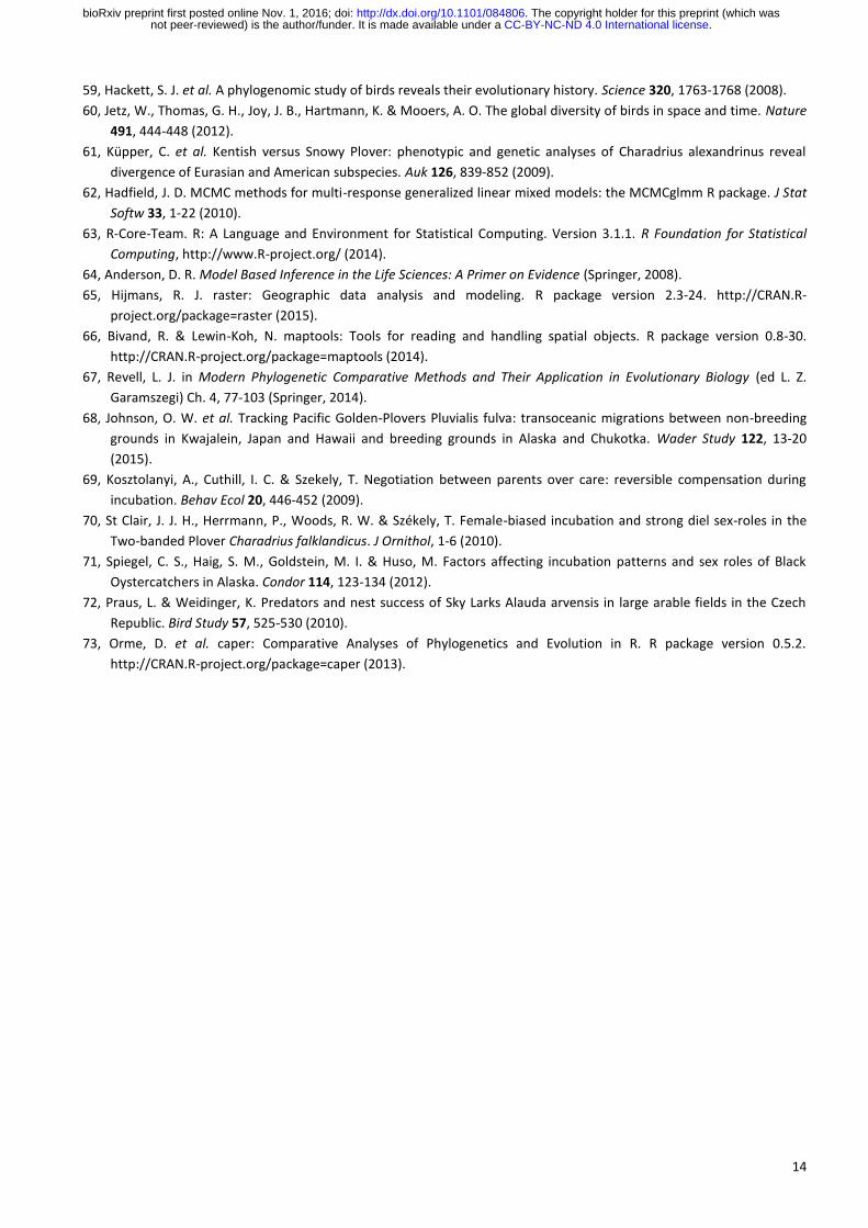
Extended Data Figure 1 | Extracting period length of incubation rhythms. a-c, Each column represents an example for a specific nest

with long, intermediate and short incubation bouts. a, From the extracted bout lengths we created a time series that indicated for each

nest, and every 10 min, whether a specific parent (female, if sex was known) incubated or not. Exchange gaps (no parent on the nest)

had to be < 6 h to be included (for treatment of exchange gaps > 6 h see d, e). b, We then estimated the autocorrelation for each 10

min time-lag up to 4 days (R ‘acf’ function63

). Positive values indicate a high probability that the female was incubating, negative values

indicate that it was more likely that the male was incubating. We used only nests that had enough data to estimate the autocorrelation

pattern (N = 584 nests from 88 populations of 30 species). The visualized autocorrelation time series never resembled white or random

noise indicative of an arrhythmic incubation pattern. To determine the period (i.e. cycle of high and low probability for a parent to

incubate) that dominated the incubation rhythm, we fitted to the autocorrelation estimates a series of periodic logistic regressions. In

each regression, the time lag (in hours) transformed to radians was represented by a sine and cosine function

, where f(t) is the autocorrelation at time-lag t, a0 is the intercept, b is the slope for sine and c the slope

for cosine, T represents the length of the fitted period (in hours), and e is an error term. We allowed the period length to vary from 0.5

h to 48 h (in 15 min intervals, giving 191 regressions). c, By comparing the Akaike’s Information Criterion64

(AIC) of all regressions, we

estimated, for each nest, the length of the dominant period in the actual incubation data (best fit). Regressions with ΔAIC (AICmodel-

AICmin) close to 0 are considered as having strong empirical support, while models with ΔAIC values ranging from 4-7 have less

support64

. In 73% of all nests, we determined a single best model with ΔAIC <= 3 (c, middle ΔAIC graph), in 20% of nests two best

models emerged and in 6% of nests 3 or 4 models had ΔAIC <= 3 (c, left and right ΔAIC graphs). However, in all but three nests, the

models with the second, third, etc. best ΔAIC were those with period lengths closest to the period length of the best model (c, left and

right ΔAIC graphs). This suggests that multiple periodicities are uncommon. d-e, The extraction of the period length (described in a-c)

requires continuous datasets, but some nests had long (>6 h) gaps between two consecutive incubation bouts, for example because of

equipment failure or because of unusual parental behaviour. In such cases, we excluded the data from the end of the last bout until the

same time the following day, if data were then available again (d), or we excluded the entire day (e).


http://dx.doi.org/10.1101/084806


16

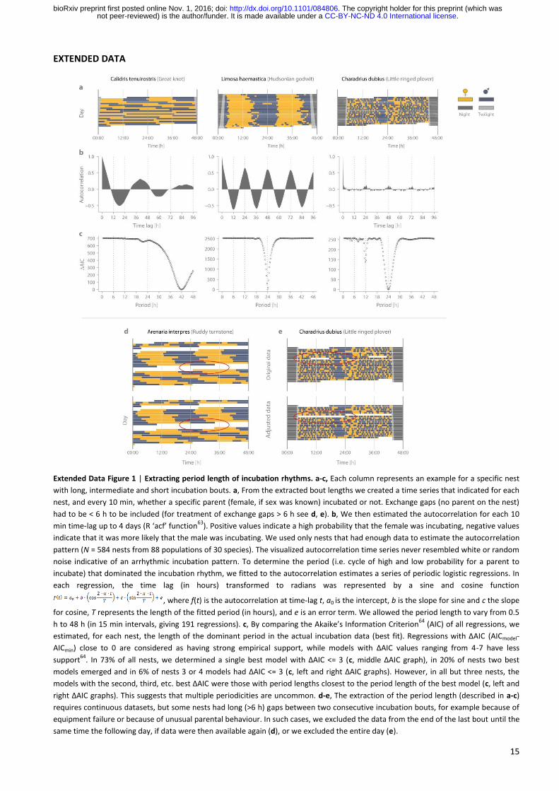
Extended Data Figure 2 | Extracting incubation bouts from light logger data. a, An example of a nest with a light intensity signal from

both parents (yellow line and blue-grey line ). The incubation bouts for a given parent reflect periods dominated by lower

light values compared to those of the partner. Note the sharp drop in the light levels at the beginning of each incubation bout and the

sharp increase in the light levels at the end. Change-overs between partners occur when the light signal lines cross. Such pronounced

changes in light intensity detected by the logger were used to assign incubation even when only a single parent was tagged. Note that

after the chicks hatch and leave the nest (July 9, vertical bar), the light intensity signal from both parents remains similar. b, An example

of a nest where one incubating parent was simultaneously equipped with a light logger and with a GPS tag. The yellow line ( )

indicates light levels, red dots ( ) indicate the distance of the bird to the nest. As expected, low light levels co-occur with close proximity

to the nest, and hence reflect periods of incubation. Although light levels decrease during twilight (light grey horizontal bar; ), the

recordings were still sensitive enough to reflect periods of incubation, i.e. the light signal matches the distance (e.g. May-25: female

incubated during dawn, but was off the nest during dusk). a-b, Rectangles in the background indicate extracted female (light yellow

polygon, ) and male (light blue-grey polygon, ) incubation bouts.


http://dx.doi.org/10.1101/084806


17

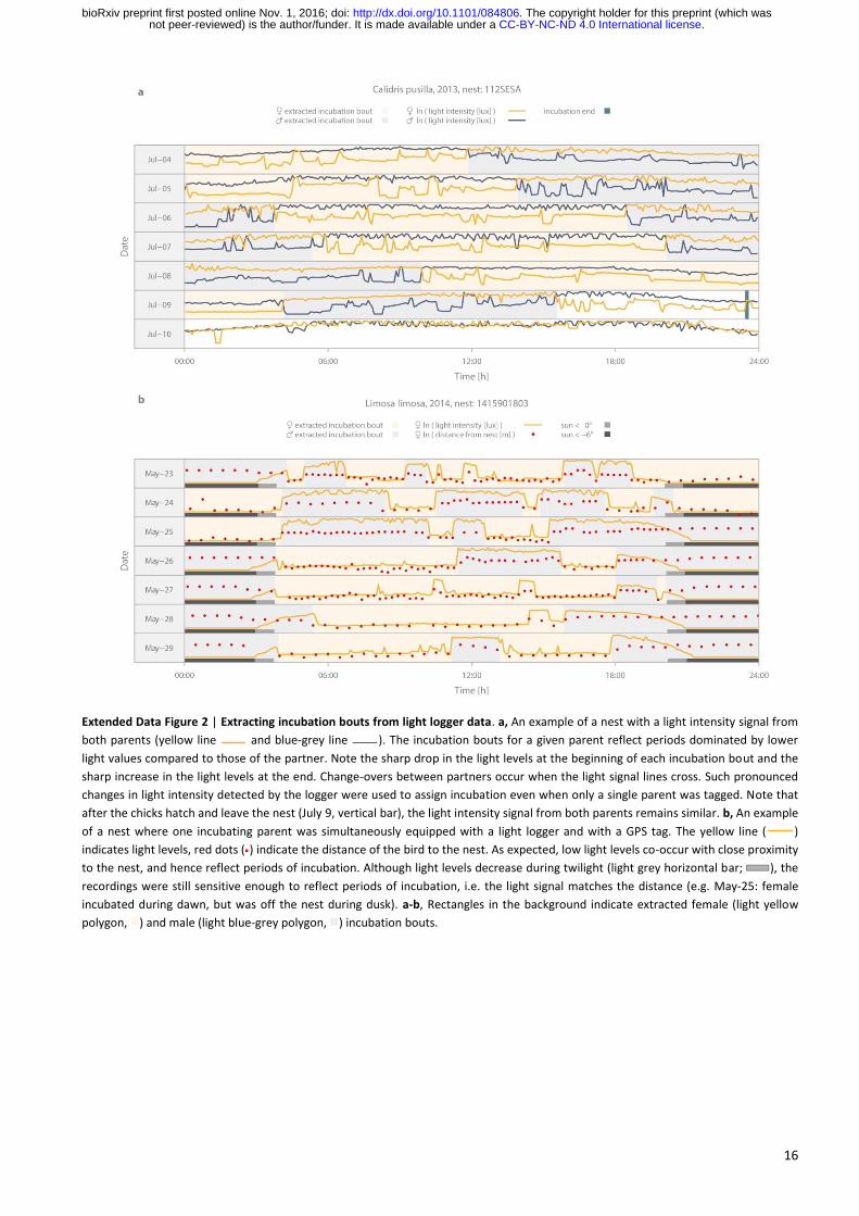
Extended Data Figure 3 | Relationship between bout and period length for 30 shorebird species. Each dot represents one nest (N =

584 nests), colours indicate the genus.


http://dx.doi.org/10.1101/084806


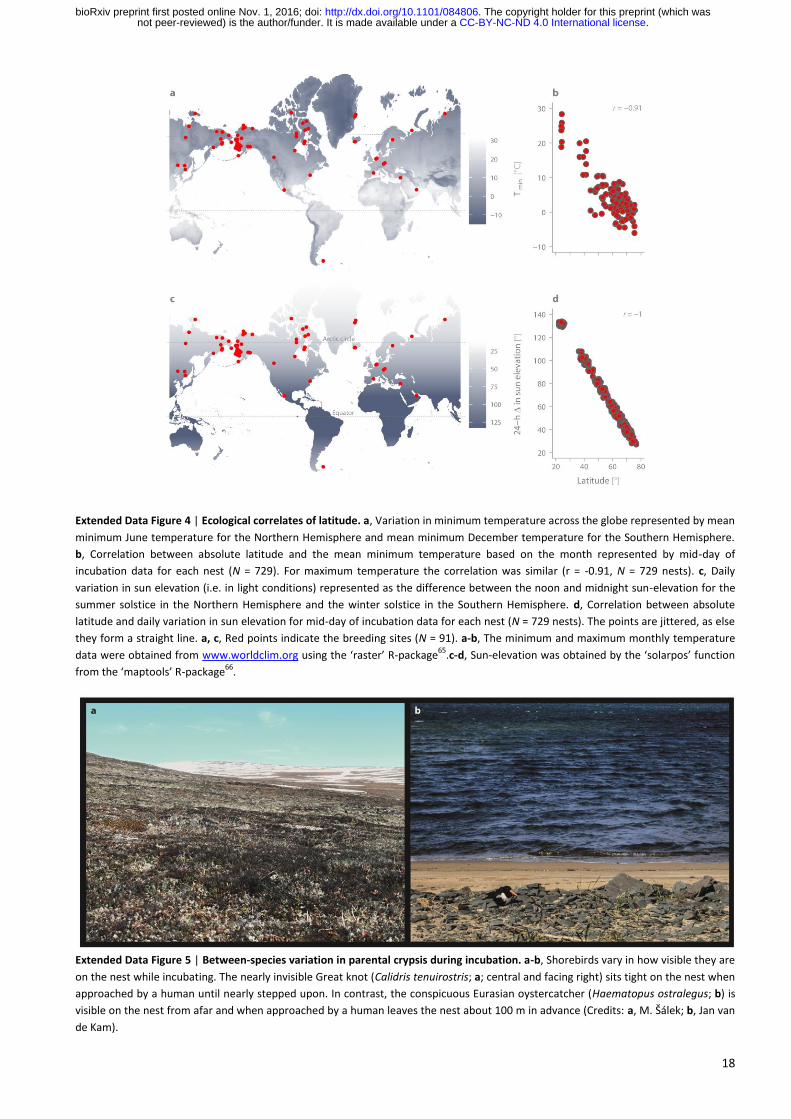
18

Extended Data Figure 4 | Ecological correlates of latitude. a, Variation in minimum temperature across the globe represented by mean

minimum June temperature for the Northern Hemisphere and mean minimum December temperature for the Southern Hemisphere.

b, Correlation between absolute latitude and the mean minimum temperature based on the month represented by mid-day of

incubation data for each nest (N = 729). For maximum temperature the correlation was similar (r = -0.91, N = 729 nests). c, Daily

variation in sun elevation (i.e. in light conditions) represented as the difference between the noon and midnight sun-elevation for the

summer solstice in the Northern Hemisphere and the winter solstice in the Southern Hemisphere. d, Correlation between absolute

latitude and daily variation in sun elevation for mid-day of incubation data for each nest (N = 729 nests). The points are jittered, as else

they form a straight line. a, c, Red points indicate the breeding sites (N = 91). a-b, The minimum and maximum monthly temperature

data were obtained from www.worldclim.org using the ‘raster’ R-package65

.c-d, Sun-elevation was obtained by the ‘solarpos’ function

from the ‘maptools’ R-package66

.

Extended Data Figure 5 | Between-species variation in parental crypsis during incubation. a-b, Shorebirds vary in how visible they are

on the nest while incubating. The nearly invisible Great knot (Calidris tenuirostris; a; central and facing right) sits tight on the nest when

approached by a human until nearly stepped upon. In contrast, the conspicuous Eurasian oystercatcher (Haematopus ostralegus; b) is

visible on the nest from afar and when approached by a human leaves the nest about 100 m in advance (Credits: a, M. Šálek; b, Jan van

de Kam).


http://www.worldclim.org/

http://dx.doi.org/10.1101/084806


19

Extended Data Figure 6 | Phylogenetic relationships for predictors. a, Body size, estimated as female wing length. b, Latitude

(absolute), c, Escape distance. a-c, We visualised the evolution of these traits29,67

using species’ medians (a-b; based on population

medians), species’ estimates of escape distance (c) and one of the 100 sampled trees (see Methods).


http://dx.doi.org/10.1101/084806


20

Extended Data Table 1 | Incubation monitoring methods and systems.

For details about methods used in each populations, see Supplementary Data53

.

*At one nest a bird with MK logger was recaptured and the logger exchanged for Intigeo logger. This nest appears in N for both logger

types.

**Simultaneously equipped with light logger (Intigeo). This nest appears in N for both GPS-tracer and Intigeo.


http://dx.doi.org/10.1101/084806


21

Extended Data Table 2 | Effects of phylogeny and sampling on bout length and period length.

The posterior estimates (modes) of the effect sizes with the highest posterior density intervals (95% CI) and the median and range of

the effective sample sizes (N (range)) come from the joint posterior distribution of 100 separate runs each with one of 100 separate

phylogenetic trees from http://birdtree.org. Nbout = 729 nests from 91 populations belonging to 32 species. Nperiod = 584 nests from 88

populations belonging to 30 species. Sampling (how often the incubation behaviour was sampled) was ln-transformed and then mean-

centred and scaled (divided by SD). For procedures and specifications related to phylogenetic Bayesian mixed models see Methods.

Estimating Pagel’s λ on the species level (Nbout = 32 species, Nperiod = 30 species) with phylogenetic generalized least-squares using the

function ‘pgls’ from the R-package ‘caper’73

gave similar results (median (range) λbout = 0.73 (0.63-1) and λperiod = 0.95 (0.64-1), based on

100 estimates each for one of the 100 trees).

Extended Data Table 3 | Source of phylogenetic signal

The posterior estimates (modes) of the effect sizes with the highest posterior density intervals (95% CI) and the effective sample sizes

(N) come from a posterior distribution of 1,100 simulated values generated by ‘MCMCglmm’ in R62

. Nbout = 729 nests from 91

populations belonging to 32 species. Nperiod= 584 nest from 88 populations belonging to 30 species.


http://dx.doi.org/10.1101/084806


22

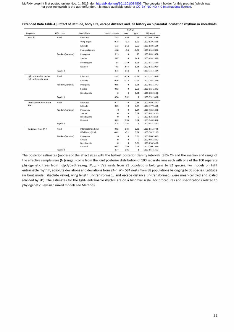
Extended Data Table 4 | Effect of latitude, body size, escape distance and life history on biparental incubation rhythms in shorebirds

The posterior estimates (modes) of the effect sizes with the highest posterior density intervals (95% CI) and the median and range of

the effective sample sizes (N (range)) come from the joint posterior distribution of 100 separate runs each with one of the 100 separate

phylogenetic trees from http://birdtree.org. Nbout = 729 nests from 91 populations belonging to 32 species. For models on light

entrainable rhythm, absolute deviations and deviations from 24-h: N = 584 nests from 88 populations belonging to 30 species. Latitude

(in bout model: absolute value), wing length (ln-transformed), and escape distance (ln-transformed) were mean-centred and scaled

(divided by SD). The estimates for the light- entrainable rhythm are on a binomial scale. For procedures and specifications related to

phylogenetic Bayesian mixed models see Methods.


http://dx.doi.org/10.1101/084806


Documents

Bulla et al 2016 Unexpected diversity in socially ... · 1 Unexpected diversity in socially synchronized rhythms of shorebirds . Martin Bulla. 1, Mihai Valcu. 1, Adriaan M. Dokter