Embed Size (px)
Citation preview
Bulk viscosity and the phase transition of the linear sigma model
Antonio Dobado*
Departamento de Fısica Teorica I, Universidad Complutense de Madrid, 28040 Madrid, Spain
Juan M. Torres-Rincon†
School of Physics and Astronomy, University of Minnesota, Minneapolis, Minnesota 55455, USA‡
(Received 12 June 2012; published 15 October 2012)
In this work, we deal with the critical behavior of the bulk viscosity in the linear sigma model (L�M) as
an example of a system which can be treated by using different techniques. Starting from the Boltzmann-
Uehling-Uhlenbeck equation, we compute the bulk viscosity over entropy density of the L�M in the
large-N limit. We search for a possible maximum of �=s at the critical temperature of the chiral phase
transition. The information about this critical temperature, as well as the effective masses, is obtained
from the effective potential. We find that the expected maximum (as a measure of the conformality loss) is
absent in the large-N limit in agreement with other models in the same limit. However, this maximum
appears when, instead of the large-N limit, the Hartree approximation within the Cornwall-Jackiw-
Tomboulis formalism is used. Nevertheless, this last approach to the L�M does not give rise to the
Goldstone theorem and also predicts a first-order phase transition instead of the expected second-order
one. Therefore, both the large-N limit and the Hartree approximations, should be considered relevant and
informative for the study of the critical behavior of the bulk viscosity in the L�M.
DOI: 10.1103/PhysRevD.86.074021 PACS numbers: 51.20.+d, 25.75.�q, 25.75.Nq
I. INTRODUCTION
Transport properties are essential to understand theequilibration of the hadronic matter created at heavy-ioncolliders. In this context, the most studied transport coef-ficient has been the shear viscosity �. When two relativis-tic nuclei collide, the initial spatial anisotropy of theinteracting region is converted into momentum anisotropydue to the hydrodynamical evolution. The momentum-anisotropy equilibration is mainly controlled by the shearviscosity, and it influences the value of the flow coefficientsvn. Comparing the measured value of the elliptic flowv2 [1,2] with the numerical hydrodynamic simulations, avalue of�=s ’ 0:1 has been estimated [3–5] (where s is theentropy density). This small value, very close to theKovtun, Son, and Starinets (KSS) minimum conjecturedin Ref. [6], has characterized the matter created in relativ-istic heavy-ion collisions as a nearly perfect fluid. It hasalso been shown that the KSS coefficient �=s has a mini-mum at the liquid-gas phase transition of common fluids[7,8]. A minimum near the phase transition of the linearsigma model (L�M) in the large-N limit has also beenfound [9], and this minimum is also expected in the de-confinement phase transition of QCD [8,10].
Another transport coefficient which relates momentumflux with a velocity gradient is the bulk viscosity � . It issensitive to uniform expansions of the system in such away that it is closely related to the scale invariance of the
fluid [11,12]. For conformal systems, the bulk viscosityidentically vanishes. This coefficient has been assumed tobe much smaller than the shear viscosity as is the case forcommon fluids. Moreover, in perturbative QCD, the ratiobetween the bulk viscosity and the shear viscosity has beenestimated around 10�3–10�8 [13]. In the low temperaturephase, the hadronic medium, this coefficient has beencalculated using the Green-Kubo formalism and kinetictheory in Refs. [14,15], respectively. In this phase, the ratio�=� has been found to be around 10�3–3� 10�3 [16].However, near the critical point, � can be larger than the
shear viscosity. For those systemsbelonging to the dynamicaluniversality class of model H (like the liquid-gas transition),the bulk viscosity diverges [17] with the correlation lengthas � ’ �2:8 (or as a function of the reduced temperature[t ¼ T=Tc � 1] as � ’ t�1:8). In lattice QCD calculationsof the bulk viscosity over entropy density above the criticaltemperature [18,19], this coefficient seems to diverge at Tc.Other authors have pointed out that the bulk viscositypresents a maximum in the critical temperature for somedifferent models like the OðNÞ model, even at mean-fieldlevel [20–23]. However, this maximum at Tc is not seen inother systems as in the Gross-Neveu model in the limit of alarge number of fermion fields [24], where the bulk viscosityis a monotonically decreasing function when temperatureincreases. In the context of the OðNÞ model, it has beenrecently shown [25] that it belongs to model C if N ¼ 1and tomodelG ifN > 1 (particularly, the large-N limit) witha divergence with the correlation length if N¼1 going as� � �2 and being finite for N > 1 as � � �0.In the hydrodynamic calculations of relativistic heavy-
ion collisions, the bulk viscosity over entropy density can
*[email protected]†[email protected], [email protected]‡On leave of absence from Departamento de Fısica Teorica I,
Universidad Complutense de Madrid, 28040 Madrid, Spain.
PHYSICAL REVIEW D 86, 074021 (2012)
1550-7998=2012=86(7)=074021(21) 074021-1 � 2012 American Physical Society

also be extracted. For example, in Ref. [5], it is found that avalue �=s ¼ 0:04 is compatible with the integrated ellipticflow measured by RHIC and ALICE collaborations. InRef. [26], a similar value is found (�=s & 0:05) near thefreeze-out temperature.
In principle, our goal is to study the behavior of the bulkviscosity over entropy density in the L�M in the large-Nlimit following the same lines of our previous article [9].We will compare the phase diagram of the L�M in thelarge-N limit with the coefficient �=s in order to ascertainif a maximum of �=s is found near Tc. In Sec. II, we presentthe L�M and its effective potential at finite temperaturein the large-N limit. In Sec. III, we review the calculationof the shear viscosity over entropy density in this model. InSec. IV, we will perform the detailed computation of thebulk viscosity over entropy density and discuss the resultsin terms of the conformality loss of the system. In Sec. V,we repeat the calculation for �=s in the context of theCornwall-Jackiw-Tomboulis (CJT) formalism in theHartree approximation. Finally, in Sec. VI, we presentour main conclusions.
II. L�M LAGRANGIAN IN THE LARGE-N LIMIT
In this section, we will review the dynamics of the L�Mat finite temperature, deriving the effective potential in thelarge-N limit. As we have already detailed this procedurein Ref. [9], we will only sketch the key steps of thecalculation.
The bare Euclidean Lagrangian of the L�M reads [27]
L ¼ 1
2@��
T@��� ��2�T�þ �
Nð�T�Þ2 � ��Nþ1;
(1)
where the multiplet� ¼ ð�i; �Þ (i ¼ 1,N) containsN þ 1scalar fields. � is positive in order to have a potentialbounded from below, and we consider ��2 to be positivein order to provide a spontaneous symmetry breaking(SSB). When � ¼ 0, the SSB pattern is SOðN þ 1Þ !SOðNÞ. In the following, we will refer for historical rea-sons to the � fields as pions (even if it is well establishedthat the L�M is not an accurate model for chiral dynamics)and to the � related degree of freedom as the Higgs.
The factor � ¼ m2�f� is responsible for the physical
pion mass, and, as it is well known, it gives rise to anexplicit breaking of the SOðN þ 1Þ symmetry. In the limitT ¼ 0, the potential has a nonzero vacuum expectationvalue (VEV), and one expects SSB. Choosing the VEV,which will be denoted by f�, pointing in the N þ 1 direc-tion, we get the equation
� 2 ��2f� þ 4�
Nf3� � � ¼ 0: (2)
For small �, the solution to this equation is
f� ¼ffiffiffiffiffiffiffiffiffiffiN ��2
2�
sþ �
4 ��2¼ f�ð� ¼ 0Þ þ �
4 ��2: (3)
The VEV can be written in terms of the N-independentF parameter defined as
h�T�i ¼ h�2ðT ¼ 0Þi ¼ f2� ¼ NF2: (4)
In our notation, we will call f�ð� ¼ 0Þ and f� the VEVat T ¼ 0 for the cases without and with an explicit sym-metry breaking term, respectively. In the next sections, theVEV at arbitrary temperature will be denoted by vðTÞ, insuch a way that f� ¼ vðT ¼ 0Þ.At T ¼ 0, the low-energy dynamics is controlled by
the broken phase. In this case, h�ai ¼ 0. Then, the relevantdegrees of freedom are the pions which correspond tothe (pseudo) Goldstone bosons when (� � 0) � ¼ 0.Fluctuations along the � direction will be denoted by ~�,and they correspond to the Higgs, the massive mode whichis relevant at higher energies (or temperatures):
� ¼ f� þ ~� ! h�i ¼ f�: (5)
The Lagrangian (1) written in terms of �a, f� and ~�reads
L ¼ 1
2@��
a@��a þ 1
2@� ~�@� ~�� ��2�a�a � ��2 ~�2
þ �
N½2f2�ð�a�a þ 3 ~�2Þ þ ð�a�aÞ2 þ 2�a�a ~�2
þ ~�4 þ 4f� ~�3 þ 4�a�af� ~��
þ���þ 4�
Nf3� � 2 ��2f�
�~�
� ��2f2� þ �
Nf4� � �f�: (6)
Note that the tadpole term vanishes because of Eq. (2).The tree-level Higgs mass can be read from the Lagrangianin Eq. (6):
M2~� ¼ �2 ��2 þ 12�
Nf2�; (7)
and it can also be written as
M2~� ¼ 4 ��2 þ 3
�
f�¼ 8�f2�
Nþ �
f�’ 8�f2�ð� ¼ 0Þ
Nþ 3
�
f�;
(8)
using Eq. (3) for the last identity.The pion mass reads
m2� ¼ �2 ��2 þ 4�
Nf2�; (9)
which, as expected, depends only on the explicit symmetrybreaking term
m2� ¼ �
f�; (10)
ANTONIO DOBADO AND JUAN M. TORRES-RINCON PHYSICAL REVIEW D 86, 074021 (2012)
074021-2

and vanishes when � ¼ 0 (obviously all pions are degen-erate). The pion and Higgs masses are related through
M2~� ¼ m2
� þ 8�f2�N
: (11)
For small enough explicit symmetry breaking, we have
�� 2 ¼ M2~� � 3m2
�
4; (12)
� ¼ N
8f2�ðM2
~� �m2�Þ: (13)
Equation (13) can be expressed in terms of the VEVat � ¼ 0:
� ¼ N
8f2�ð� ¼ 0ÞM2
~� �m2�
2; (14)
where is a multiplicative constant relating f� andf�ð� ¼ 0Þ,
f� ¼ f�ð� ¼ 0Þ; (15)
which can be written as
¼ M2~� � 3m2
�
M2~� � 4m2
�
; (16)
where we have used Eq. (3) and consider small �.In order to obtain the effective potential, we will inte-
grate out the fluctuations from the partition function Z. Todo that, it is convenient to introduce an auxiliary scalarfield. This field allows for a systematic counting of Nfactors and provides some simplifications in the large-Nlimit. Then, the integration of the pions and the Higgs isperformed by standard Gaussian integration.
The integration of the fluctuations is done regardless oftheir wavelengths. All the frequency modes of the scalarfields are treated at the same footing, and this ‘‘unorganized’’integration produces two undesirable features in the effectivepotential. First, an imaginary part of the effective potentialappears. This imaginary part has been given the interpreta-tion of a decay rate per unit volume of the unstable vacuumstate by Weinberg and Wu in Ref. [28].
The second characteristic is the nonconvexity of thequantum effective potential. However, the effective poten-tial, defined through a Legendre transformation of thegenerating functional of the connected diagrams [29],should always be convex. This nonconvexity problem andthe imaginary part appear as long as a perturbative methodis used to calculate the effective potential [30].
A possible solution for these problems can be given byusing a nonperturbative method to generate the effectivepotential. For example, the functional renormalizationgroup generates an effective potential in such a way thatan organized integration of the fluctuations is performed.Following the ideas of the renormalization group, only thelow-wavelength components of the quantum fluctuations
are integrated out at each step. Thus, the UV componentsare infinitesimally integrated step by step, and the finaleffective potential (defined in the infrared scale) does notacquire an imaginary part, and it remains convex at everyscale (at the IR point, the Maxwell construction is dynami-cally generated by the renormalization flow) [31].In spite of the previous discussion, we understand that it
is not necessary to perform a more sophisticated method toobtain the effective potential. The only relevant informa-tion for us is the location of the effective potential mini-mum, which eventually gives the position of the criticaltemperature. This minimum appears always outside of thenonconvex region. On the other hand, the possible presenceof an imaginary part (whose domain in fact coincides withthe domain of the nonconvex part of the effective potential)is not relevant for us in this work.
A. Auxiliary field method and effectivepotential at T � 0
To compute the effective potential in the large-N limit,we start by considering the partition function:
Z ¼Z
D�aD� exp
��Z
d4xL�; (17)
with the Lagrangian of Eq. (1). Then, we introduce anauxiliary field in order to deal with the quartic couplingby using the Gaussian integral:
exp
��Zd4x
�
N�4
�/ZDexp
�Zd4x
�N
8�2�
ffiffiffi2
p2�2
��:
(18)
To prove the equivalence between the two Lagrangians,note that this auxiliary field has introduced a mass term anda coupling with �2 in the Lagrangian. However, it has nokinetic term which means that has not a true dynamics.
The Euler-Lagrange equation for simply gives ¼2
ffiffiffi2
p��2=N. Introducing this solution into the right-hand
side of Eq. (18), one obtains the Lagrangian
L ¼ � N
8�2 þ
ffiffiffi2
p2
�2 ¼ � �
N�4 þ 2
�
N�4 ¼ �
N�4;
(19)
which is the original interaction Lagrangian.The partition function can then be written as
Z ¼Z
D�aD�D exp
��Z
d4x
�1
2@��
a@��a
þ 1
2@��@
��� ��2�a�a � ��2�2 � N
8�2
þffiffiffi2
p2
�a�a þffiffiffi2
p2
�2 � ��
��:
BULK VISCOSITY AND THE PHASE TRANSITION OF . . . PHYSICAL REVIEW D 86, 074021 (2012)
074021-3
Thus the action in terms of the �a, �, and fields reads
S ¼Z
d4x
�1
2�að�hE � 2 ��2 þ ffiffiffi
2p
Þ�a
þ 1
2�ð�hE � 2 ��2 þ ffiffiffi
2p
�� N
8�2 � ��
�: (20)
Before identifying properly the pion propagator, one mustget rid of the unphysical � tadpole. We have already seenthat this term vanishes at T ¼ 0. Now, we perform a shift ofthe � field � ¼ vþ ~� which also produces a change in the
auxiliary field ¼ ~þ 2ffiffiffi2
p�N v
2 þ 4ffiffiffi2
p�N v~� allowing us
to cancel the tadpole term for ~� and the unphysical massmixing term between ~� and ~. After some manipulations,we obtain the action
S¼Zd4x
�1
2�að�hEþG�1
� ½0;�Þ�a
þ 1
2~�
��hEþG�1
� ½0;�þ 8�
Nv2
�~�þ 1
2v2G�1
� ½0;�
� N
8�~2�
ffiffiffi2
p2v2þ �
Nv4� �v
�; (21)
where we have introduced the function
G�1� ½q; � � q2 � 2 ��2 þ ffiffiffi
2p
: (22)
Now comes our approximation for the auxiliary field. isnot going to be integrated out, but treated at mean-fieldlevel, so that it contains no fluctuations. In particular, weapply this simplification for the quadratic term in the action.At mean field (note that we will keep the same notation ,instead of using hi as they coincide in this approximation),
~ ¼ � 2ffiffiffi2
p �
Nv2: (23)
So the quadratic term reads
� N
8�~2 ¼ � N
8�2 þ
ffiffiffi2
p2
v2� �
Nv4: (24)
The last two factors are cancelled in the action (20). We aregoing to trade byG�1
� ½0; �. Using Eq. (22), the quadraticterms is
� N
8�2 ¼ � N
16�ðG�1
� ½0; �Þ2 � N
4���2G�1
� � N
4���4:
(25)
We will neglect the last term in the action because it is aconstant. Finally, we use the relations
N ��2
4�¼ f2�ð� ¼ 0Þ
2¼ f2�
22¼ NF2
2; (26)
to introduce F ¼ vðT ¼ 0Þ, i.e., the VEV at zerotemperature.
The final action becomes
S½�a;v; ~�;G�1� ½0;��¼
Zd4x
�1
2�að�hEþG�1
� ½0;�Þ�a
þ1
2~�
��hEþG�1
� ½0;�þ8�
Nv2
�~�
þ1
2v2G�1
� ½0;��NF2
22G�1
� ½0;�
� N
16�ðG�1
� ½0;�Þ2��v
�: (27)
Notice that G�1� ½q; � is nothing but the inverse of the
pion propagator in Fourier space. The inverse propagatorof the ~� field is
G�1~� ½q; � ¼ G�1
� ½q; � þ 8�
Nv2: (28)
In order to generate the effective potential for v, we nowintegrate out the fluctuations. By performing a standardGaussian integration of the pions, we get
ZD�a exp
��Z
d4x1
2�a½�hE þG�1
� ½0; ���a
�
¼Z
d4x exp
�N
2
ZTXn2Z
d3q
ð2�Þ3 logG�1� ½q; �
�; (29)
where q0 ¼ 2�nT is the well-known Matsubara frequencyappearing in finite temperature computations. The sameprocedure can be applied to integrate out ~�. To be able toperform the integrations , we have assumed that the aux-iliary field (or G�1
� ½0; �) is homogeneous, i.e., it does notdepend on x. This assumption is also taken for the VEVofthe � field and allows us to obtain a simple representationin Fourier space, where different modes do not mixbetween them and the integration is straightforward.The effective potential (density) reads
Veffðv;G�1� ½0; �Þ ¼ 1
2
�v2 � NF2
2
�G�1
� ½0; �
� N
16�ðG�1
� ½0; �Þ2 � �v
þ N
2
ZX�logG�1
� ½q; �
þ 1
2
ZX�logG�1
~� ½q; �; (30)
with
ZX�¼ T
Xn2Z
Z d3q
ð2�Þ3 : (31)
Looking at the N power counting of the different termsin the effective potential, one finds that all of them behaveas OðNÞ except the last one. Therefore, the contribution ofthe Higgs to the effective potential is suppressed in thelarge-N limit by one power ofN, and it will be neglected inthe following. Then, the effective potential becomes
ANTONIO DOBADO AND JUAN M. TORRES-RINCON PHYSICAL REVIEW D 86, 074021 (2012)
074021-4
Veffðv;G�1� ½0; �Þ ¼ 1
2
�v2 � NF2
2
�G�1
� ½0; �
� N
16�ðG�1
� ½0; �Þ2 � �v
þ N
2
ZX�logG�1
� ½q; �: (32)
The last term needs to be regulated because it contains adivergence. This divergence can be absorbed by a properrenormalization of the quartic coupling [9]. Thus, therenormalized (�-independent) effective potential finallyreads
Veffðv;G�1½0; �Þ ¼ 1
2
�v2 � NF2
2
�G�1
� ½0; � � �v
� N
2g0ðT;G�1
� ½0; �Þ
� N
16ðG�1
� ½0; �Þ2�
1
�Rð�Þ� 1
4�2log
� ffiffiffie
pG�1
� ½0; ��2
��; (33)
where the function g0ðT;G�1� ½0; �Þ is defined in
Appendix A.
The stationary conditions are given by
dVeff
dG�1� ½0; �
��������G�1� ½0;�¼G�1
�;0½0;�
¼ 0;dVeff
dv
��������v¼v0
¼ 0;
(34)
and they provide G�1�;0½0; � and the order parameter v0 in
this approximation. The effective mass of the pion isobtained as m2
� ¼ G�1�;0½0; �, and the effective Higgs
mass as M2R ¼ G�1
�;0½0; � þ 8 �N v
20, which has the same
form as Eq. (11).For the � ¼ 0 case, there is no explicit symmetry-
breaking term, and we expect to have a second-order
phase transition defined by the critical temperature Tc ¼ffiffiffiffiffiffi12
pF ¼ ffiffiffiffiffiffiffiffiffiffiffiffi
12=Np
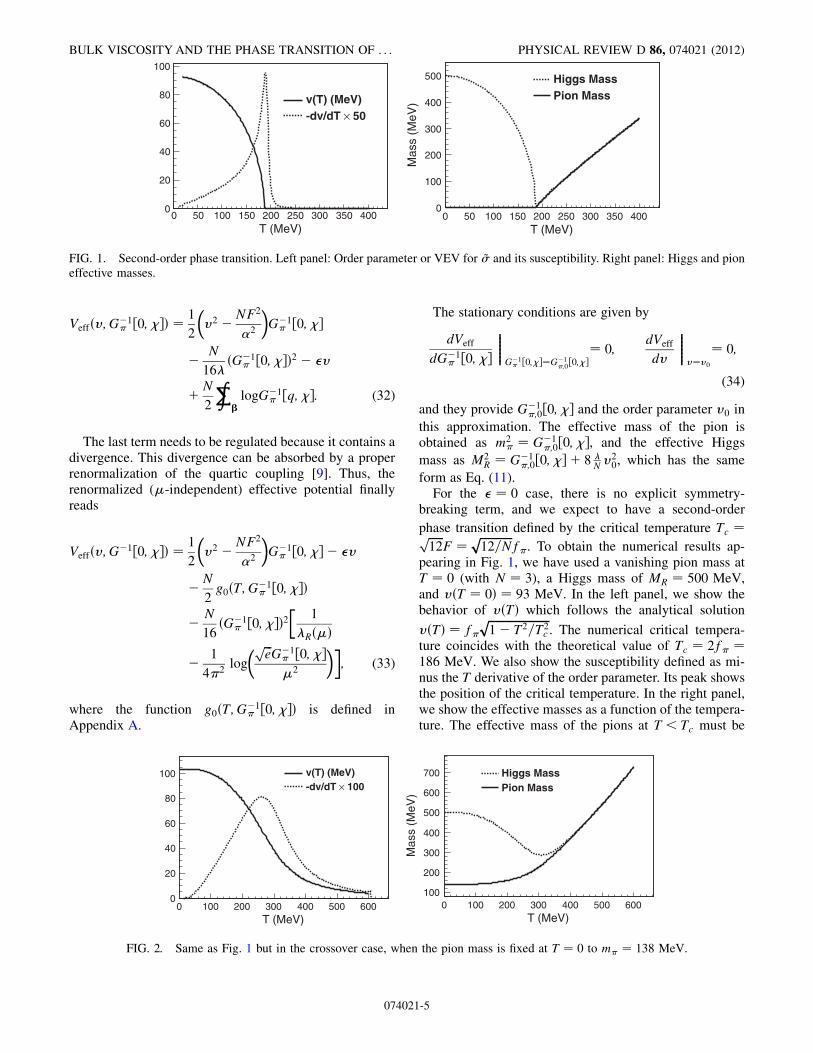
f�. To obtain the numerical results ap-pearing in Fig. 1, we have used a vanishing pion mass atT ¼ 0 (with N ¼ 3), a Higgs mass of MR ¼ 500 MeV,and vðT ¼ 0Þ ¼ 93 MeV. In the left panel, we show thebehavior of vðTÞ which follows the analytical solution
vðTÞ ¼ f�ffiffiffiffiffiffiffiffiffiffiffiffiffiffiffiffiffiffiffiffiffiffi1� T2=T2
c
p. The numerical critical tempera-
ture coincides with the theoretical value of Tc ¼ 2f� ¼186 MeV. We also show the susceptibility defined as mi-nus the T derivative of the order parameter. Its peak showsthe position of the critical temperature. In the right panel,we show the effective masses as a function of the tempera-ture. The effective mass of the pions at T < Tc must be
T (MeV)0 50 100 150 200 250 300 350 400
0
20
40
60
80
100
v(T) (MeV) 50×-dv/dT
T (MeV)0 50 100 150 200 250 300 350 400
Mas
s (M
eV)
0
100
200
300
400
500 Higgs MassPion Mass
FIG. 1. Second-order phase transition. Left panel: Order parameter or VEV for ~� and its susceptibility. Right panel: Higgs and pioneffective masses.
T (MeV)
0
20
40
60
80
100 v(T) (MeV) 100×-dv/dT
T (MeV)0 100 200 300 400 500 600 0 100 200 300 400 500 600
Mas
s (M
eV)
100
200
300
400
500
600
700 Higgs MassPion Mass
FIG. 2. Same as Fig. 1 but in the crossover case, when the pion mass is fixed at T ¼ 0 to m� ¼ 138 MeV.
BULK VISCOSITY AND THE PHASE TRANSITION OF . . . PHYSICAL REVIEW D 86, 074021 (2012)
074021-5

always zero according to the Goldstone theorem (numeri-cally, it is fixed at 0.5 MeV at T ¼ 0 in order to avoidcomputational problems). At Tc, it starts growing withtemperature in the symmetric phase. The effective massof the Higgs follows the same pattern as the order parame-ter becoming zero at Tc. For higher temperatures, it in-creases until being degenerate with the effective pion massas expected because of the restoration of the SOðN þ 1Þsymmetry.
For the � � 0 case, a crossover instead of a real phasetransition is expected (this is the same situation as addingan external magnetic field to a ferromagnet). We fix m� ¼138 MeV at zero temperature and the same values for MR
and f� taken for the � ¼ 0 case. The results are shown inFig. 2. The left panel shows the order parameter vðTÞwhich decreases with temperature and never becomesexactly zero. The crossover temperature can be definedas the position of the peak in the susceptibility which weplot in dotted line. In the right panel, we show the pionthermal mass (solid line) and the Higgs mass (dotted line).They are degenerate for high temperatures.
III. SHEARVISCOSITYOVER ENTROPYDENSITY
The shear viscosity for the L�M was obtained inRef. [9]. In the following, we will briefly review themethod used there with some minimal changes. The trans-port equation for the one-particle distribution functionfpðt;xÞ is
dfpðt;xÞdt
¼ C½fp�: (35)
Taking into account only elastic collisions (we will discusslater the influence of inelastic terms), this equation reads
@fpðt;xÞ@t
þ p
Ep
� rfpðt;xÞ ¼ N
2
Zd�12;3p½f1f2ð1þ f3Þ
� ð1þ fpÞ � f3fpð1þ f1Þ� ð1þ f2Þ�; (36)
where
d�12;3p¼ 1
2Ep
Y3i¼1
dki
ð2�Þ32Ei
jTj2ð2�Þ4�ð4Þðk1þk2�k3�pÞ:
(37)
At first order in the Chapman-Enskog expansion, the dis-tribution function is expressed as the local equilibriumdistribution function plus a small correction:
fp ¼ np þ fð1Þp ; (38)
where np is the local Bose-Einstein distribution function
npðt;xÞ ¼ 1
epuðt;xÞ��ðt;xÞ
Tðt;xÞ � 1: (39)
The Boltzmann-Uehling-Uhlenbeck (BUU) equation is
then linearized in fð1Þp :
Ep
@npðt;xÞ@t
þ p � rnpðt;xÞ
¼ �NEp
2
Zd�12;3pð1þ n1Þð1þ n2Þn3np
�fð1Þ3
n3ð1þ n3Þ
þ fð1Þp
npð1þ npÞ �fð1Þ1
n1ð1þ n1Þ �fð1Þ2
n2ð1þ n2Þ�: (40)
The left-hand side depends only on the space-time deriva-tives of np, which can be explicitly obtained using the
Euler and continuity equations.The shear viscosity can be also expressed in terms
of fð1Þp :
2� ~Vij ¼ NZ d3p
ð2�3ÞEp
fð1Þp pipj; (41)
where ~Vij ¼ @iVj þ @jVi � 13�ijr � V is the shear gra-
dient of the velocity field.The left-hand side of the BUU equation also carries the
same gradient (neglecting the influence of other transportcoefficients),
Ep
@npðt;xÞ@t
þp �rnpðt;xÞ¼�npð1þnpÞpipj ~Vij: (42)
In order to cancel out this factor from the BUU equation
and also from Eq. (41), the function fð1Þp is taken as
fð1Þp ¼ �npð1þ npÞ�3BðpÞpipj ~Vij; (43)
with BðpÞ being an unknown function of p. InsertingEq. (43) into Eq. (41), one gets
� ¼ N
30�2T3
Zdp
p6
Ep
npð1þ npÞBðpÞ: (44)
It is convenient to write this formula in terms of theadimensional variables
x ¼ Ep
m�
; y ¼ m�
T: (45)
Introducing the integration measure d��ðx; yÞ defined inAppendix B, we find
� ¼ Nm6�
30�2T3
Z�d��ðx; yÞBðxÞ: (46)
This BðxÞ function can be expanded in terms of thepolynomial basis PnðxÞ defined in Appendix B:
BðxÞ ¼ X1n¼0
bnPnðxÞ: (47)
By projecting the BUU equation into the space gener-ated by Pn, one gets
ANTONIO DOBADO AND JUAN M. TORRES-RINCON PHYSICAL REVIEW D 86, 074021 (2012)
074021-6

K0�l0 ¼XNn¼0
bnC�nl; (48)
where the functions Ki are also defined in Appendix B.The collision integrals read
C�nl¼N�2
4m2�T
2
Z Y4m¼1
d3kmð2�Þ32Em
jTj2ð2�Þ4
��ð4Þðk1þk2�k3�pÞð1þn1Þð1þn2Þn3np��pipj
m2�
PlðpÞþk3ik3j
m2�
Plðk3Þ�k1ik1j
m2�
PlðK1Þ
�k2ik2j
m2�
Plðk2Þ��
pipj
m2�
PnðpÞþk3ik3j
m2�
Pnðk3Þ
�k1ik1j
m2�
Pnðk1Þ�k2ik2j
m2�
Pnðk2Þ�: (49)
At the lowest order in the expansion (47), the shearviscosity can be written as
� ¼ Nm6�
30�2T3
K20
C�00; (50)
where the pion effective mass m� is now taken from thegap equations of the effective potential and
C�00 ¼N�2
4m2�T
2
Z Y4m¼1
d3kmð2�Þ32Em
jTj2ð2�Þ4
� �ð4Þðk1 þ k2 � k3 � pÞð1þ n1Þð1þ n2Þn3np�
�pipj
m2�
þ k3ik3j
m2�
� k1ik1j
m2�
� k2ik2j
m2�
�
��pipj
m2�
þ k3ik3j
m2�
� k1ik1j
m2�
� k2ik2j
m2�
�: (51)
The scattering amplitude in the large-N limit has beenextensively described in Ref. [9], which includes the tree-level �–� amplitude and its resummation in pion loops(as they are of the same order in N). The finite pion massgives rise to new couplings to the pion scattering [32], andthe corresponding amplitude should be added to the chiralone. In the large-N limit, the s-channel scattering is theleading one. As the amplitude is Oð1=NÞ, the total crosssection is Oð1=NÞ, but the average cross section (which isincluded in the collision integral) is Oð1=N2Þ.Note that, as C�nl �Oð1=NÞ, the shear viscosity is
OðN2Þ. This is expected [33] since the shear viscosity isproportional to the inverse coupling constant squared, andthis is suppressed by one power of N.The obtained numerical results for N ¼ 3, m�ðT¼0Þ¼0
and Higgs massesMR ¼ 0:2, 0.5 and 1.2 GeVare shown inFig. 3. They are similar to that appearing in our Ref. [9]where we have used a slightly different parametrization
for fð1Þp . We have found a minimum of �=s for the threecases, always greater than the KSS bound 1=ð4�Þ. However,the exact position of the minimum depends on the valueof MR.To check whether the minimum of �=s corresponds to
the location of the critical temperature, one must comparethe previous plot with the order parameter. We show this inFig. 4 at different values of FðT ¼ 0Þ. In the left panel, weshow the normalized value of vðTÞ. The position of thecritical temperature (where the order parameter firstvanishes) depends linearly on F. The same behavior isfollowed by the minimum viscosity over entropy density
T (MeV)0 50 100 150 200 250 300 350
/sη
1
10
210
310
410
mr12.dat
= 0.2 GeVRM
= 0.5 GeVRM
= 1.2 GeVRM
FIG. 3 (color online). Viscosity over entropy density in theL�M at large N for different values of MR.
T (MeV)
v(T
)/v(
0)
0
0.2
0.4
0.6
0.8
1
F40.datnorm
T (MeV)0 50 100 150 200 250 0 50 100 150 200 250
η/s
10
210
F40.datnorm
F(T=0)=40 MeV
F(T=0)=50 MeV
F(T=0)=60 MeV
FIG. 4 (color online). Comparison between the minimum of the viscosity over entropy density and the position of the criticaltemperature. The minimum is located close to it but slightly below.
BULK VISCOSITY AND THE PHASE TRANSITION OF . . . PHYSICAL REVIEW D 86, 074021 (2012)
074021-7

shown in the right panel. The position of this minimum isclose to Tc, but not exactly there (as shown in Fig. 4) butslightly below. Notice that Tc is MR-independent in thelarge-N approximation considered here.
IV. BULK VISCOSITY OVER ENTROPY DENSITY
In this section, we will perform the calculation of thebulk viscosity in the L�M in the large-N approximation.We start by considering both elastic and inelastic scatter-ings. Therefore, we do not introduce a pion chemicalpotential in the calculation, as the pion number is notconserved in principle. This fact simplifies the thermody-namics with respect to our previous work [15] since,instead of using the isochoric speed of sound vn and thecompressibility �1
� , one only needs to consider the adia-batic speed of sound,
v2S ¼
�@P
@�
�s=n
; (52)
where P is the pressure and � the energy density.Additionally, as we will use a quasiparticle description
of the scalar fields, we must introduce a nonvanishing termdm�=dT which enters in the left-hand side of the BUUequation:
p�@�npðxÞj�
¼ �npð1þ npÞ�p2
3� E2
pv2S þ Tm�
dm�
dTv2S
�r � V: (53)
Here, it is useful to define a new T-dependent parameter~m which includes the derivative of the thermal mass:
~m 2 � m2� � T2 dm
2�
dT2: (54)
Then, the left-hand side reads
p�@�npðxÞj� ¼ �npð1þ npÞ
�p2
3� v2
Sðp2 þ ~m2Þ�r � V:
(55)
The first-order Chapman-Enskog correction to the dis-
tribution function fp ¼ np þ fð1Þp is
fð1Þp ¼ �npð1þ npÞ�AðpÞr � V: (56)
The linearized BUU equation reads
npð1þ npÞ�p2
3� v2
Sðp2 þ ~m2Þ�
¼ Cel þ Cin
¼ NEp
2
Zd�12;3pð1þ n1Þð1þ n2Þn3np
� ½AðpÞ þ Aðk3Þ � Aðk1Þ � Aðk2Þ� þ Cin; (57)
where we represent by Cel the elastic collision operator andby Cin the part of the collision operator including inelastic
scattering (that we do not explicitly detail here). As wehave not fixed the pion chemical potential, this term shouldbe present in order to allow particle number changingprocesses.The stress-energy tensor ��� in presence of a thermal
mass is written as [23,26,34]
��� ¼ NZ d3p
ð2�Þ3Ep
�p�p� � u�u�T2 dm
2
dT2
�fð1Þp ;
which reduces to the usual stress-energy tensor when themass is T-independent.This new term does not modify the expression for the
bulk viscosity in terms of fð1Þp because the former onlydepends on the spatial components of the stress-energytensor, and in the local rest frame, one has ui ¼ 0.Therefore, we have
� ¼ N
T
Z d3p
ð2�Þ3Ep
npð1þ npÞAðpÞp2
3: (59)
However, this new term in the stress-energy tensor doeschange the form of the Landau-Lifschitz condition [35]�00 ¼ 0 (notice that this is the only condition, since the onefixing the particle density number out of equilibrium doesnot apply here):
�00 ¼ NZ d3p
ð2�Þ3Ep
ðp2 þ ~m2Þfð1Þp ¼ 0; (60)
As usual, this condition can be used to add a vanishingcontribution to the bulk viscosity, making much easier thecomparison with the BUU equation left-hand side (55),
� ¼ N
T
Z d3p
ð2�Þ3Ep
npð1þ npÞAðpÞ�p2
3� v2
Sðp2 þ ~m2Þ�:
(61)
Next, we consider again the same adimensional varia-bles we have used for the shear viscosity (x ¼ Ep=m�, y ¼m�=T) and also an integration measure d�� . This integra-
tion measure is described in detail in Appendix A includingits corresponding scalar product, the norm, the moments,the functions Ii, and the polynomial basis. The bulk vis-cosity is then expressed as the following scalar product:
� ¼ Nm4�
2�2ThAðxÞjP2ðxÞi� : (62)
The projected BUU equation is obtained by multiplyingboth sides of Eq. (57) by 1
4�m4�Ep
PlðxÞd3p and integrating
over the three-momentum:
hPlðxÞjP2ðxÞi¼ N
8�m4�
Zd3p
Zd�12;3pð1þn1Þð1þn2Þn3np
�PlðxÞ½AðpÞþAðp3Þ�Aðp1Þ�Aðp2Þ�þhCini: (63)
ANTONIO DOBADO AND JUAN M. TORRES-RINCON PHYSICAL REVIEW D 86, 074021 (2012)
074021-8

There is one important remark concerning the solutionof the linearized BUU. In this linearized equation, only onezero mode is present. When AðpÞ is proportional to x, theright-hand side is zero due to the energy-conservation law.However, due to the presence of the inelastic collisionoperator, the zero mode associated to the particle conser-vation (AðpÞ / 1) is absent.
In the left-hand side, it is easy to check that whereashP1jP2i ¼ 0, we have hP0jP2i � 0, which is consistentwith the previous remark. The BUU equation is solvablein the entire Hilbert space of solutions [36].
Due to arguments of final phase-space and suppressionin the large-N limit (which will be detailed later), we willnot consider the inelastic processes in the collision integraland retain only the 2 ! 2 processes. This simplificationcauses an inconsistency in the BUU equation, as the pro-jection of the BUU onto P0 gives different results on bothsides of the equation. This inconsistency is avoided bysolving the equation in the subspace perpendicular to the‘‘accidental’’ zero mode P0 ¼ 1.
Therefore, we expand the AðxÞ solution:
AðxÞ ¼ X1n¼1
anPnðxÞ: (64)
After symmetrization of the collision integral, the BUUequation finally reads
�l2kP2ðxÞk2 ¼X1n¼1
anCnl; (65)
with
Cnl ¼ N�2
4m4�
Z Y4i¼1
d3kið2�Þ32Ei
jTj2ð2�Þ4
� �ð4Þðk1 þ k2 � k3 � pÞð1þ n1Þ� ð1þ n2Þn3np�½PnðxÞ��½PlðxÞ�; (66)
where �½PnðxÞ� � PnðxÞ þ Pnðx3Þ � Pnðx1Þ � Pnðx2Þ.For l ¼ 1, one gets the identity 0 ¼ 0, which does not
determine the coefficient a1. The first nontrivial case cor-responds to l ¼ 2, for which the solution of the BUUequation reads
a2 ¼ kP2ðxÞk2C22
: (67)
By introducing it in the formula for the bulk viscosity,one finds
� ¼ Nm4�
2�2Ta2kP2ðxÞk2 ¼ Nm4
�
2�2T
�1
3� v2
S
�1
C22
�I4 � I2I3
I1
�:
(68)
In the following, we proceed to the discussion ofthe results for the bulk viscosity over entropy density.They will depend on the value of the pion mass at zero
temperature, i.e., on having a second-order phase transitionor a crossover. We will begin with the latter.
A. Crossover
We start with the explicit symmetry-breaking case, forwhich we set a nonzero pion mass at T ¼ 0. In order to getnumerical results, a possible choice could be the physicalpion mass m�ðT ¼ 0Þ ¼ 138 MeV. The effective massdepends on temperature in such a way that m�ðTÞ>m�ðT ¼ 0Þ ¼ 138 MeV. For this reason, and analogouslyto the physical pion gas in Ref. [15], the inelastic terms inthe collision operator (1 ! 3 or 2 ! 4) are suppressed bythe Boltzmann exponential factor in the final phase space
e�2m�=T (the inverses being too improbable to occur if thegas is dilute).However, the crossover case does not have a precise
definition of the ‘‘critical’’ temperature. Here, we willdefine it as the point where the minus derivative of theorder parameter (the susceptibility) peaks. From the leftpanel of Fig. 2, we obtain a value of Tcr ¼ 261 MeV.In Fig. 5, we show the squared speed of sound for
the pions together with the result from a pion gaswith a constant (temperature-independent) mass of m� ¼138 MeV. The difference between the two curves is attrib-uted to the effective mass of the quasiparticles. It is im-portant to remark here that both results correspond to thenoninteracting gas, i.e., ideal gas. The introduction ofinteractions in the thermodynamic functions (for example,through the free energy obtained from the effective poten-tial) would be inconsistent with the conception of theChapman-Enskog expansion at first order.The speed of sound turns out to be a monotonic
function of the temperature. It takes the conformal valuev2S ¼ 1=3 at T ¼ 259 MeV, very close to the crossover
temperature. By Eq. (B20), one can check that, at thisprecise point,
dm�
dT¼ m�
T: (69)
T (MeV)0 50 100 150 200 250 300 350 400
2 Sv
0.05
0.1
0.15
0.2
0.25
0.3
0.35
Pion m=m(T)
Pion m=138 MeV
Pion m=m(T)
Pion m=138 MeV
FIG. 5. v2S in the L�M at large N for the crossover case (solid
line) compared with the speed of sound of a pion mass with aconstant mass of 138 MeV.
BULK VISCOSITY AND THE PHASE TRANSITION OF . . . PHYSICAL REVIEW D 86, 074021 (2012)
074021-9
When v2S ¼ 1=3, the squared norm of the source P2
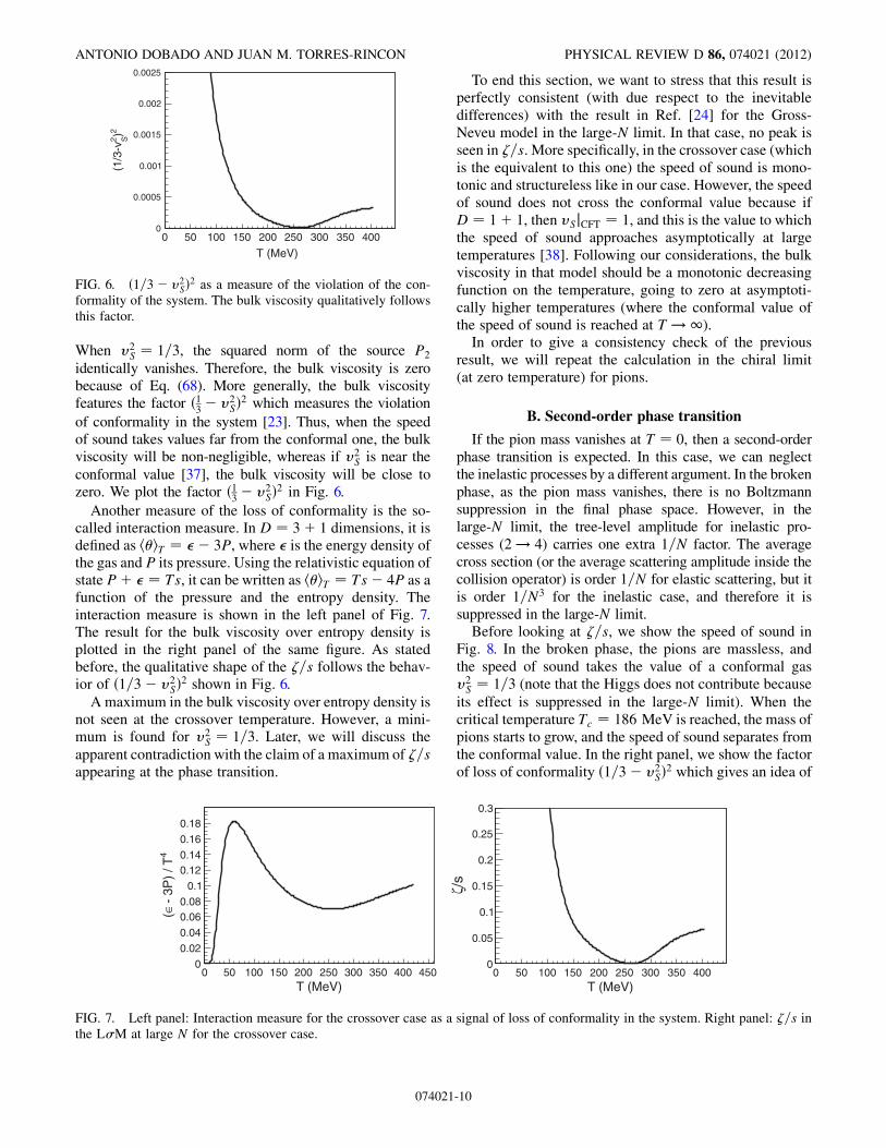
identically vanishes. Therefore, the bulk viscosity is zerobecause of Eq. (68). More generally, the bulk viscosityfeatures the factor ð13 � v2
SÞ2 which measures the violation
of conformality in the system [23]. Thus, when the speedof sound takes values far from the conformal one, the bulkviscosity will be non-negligible, whereas if v2
S is near the
conformal value [37], the bulk viscosity will be close tozero. We plot the factor ð13 � v2
SÞ2 in Fig. 6.
Another measure of the loss of conformality is the so-called interaction measure. In D ¼ 3þ 1 dimensions, it isdefined as h�iT ¼ �� 3P, where � is the energy density ofthe gas and P its pressure. Using the relativistic equation ofstate Pþ � ¼ Ts, it can be written as h�iT ¼ Ts� 4P as afunction of the pressure and the entropy density. Theinteraction measure is shown in the left panel of Fig. 7.The result for the bulk viscosity over entropy density isplotted in the right panel of the same figure. As statedbefore, the qualitative shape of the �=s follows the behav-ior of ð1=3� v2
SÞ2 shown in Fig. 6.
A maximum in the bulk viscosity over entropy density isnot seen at the crossover temperature. However, a mini-mum is found for v2
S ¼ 1=3. Later, we will discuss the
apparent contradiction with the claim of a maximum of �=sappearing at the phase transition.
To end this section, we want to stress that this result isperfectly consistent (with due respect to the inevitabledifferences) with the result in Ref. [24] for the Gross-Neveu model in the large-N limit. In that case, no peak isseen in �=s. More specifically, in the crossover case (whichis the equivalent to this one) the speed of sound is mono-tonic and structureless like in our case. However, the speedof sound does not cross the conformal value because ifD ¼ 1þ 1, then vSjCFT ¼ 1, and this is the value to whichthe speed of sound approaches asymptotically at largetemperatures [38]. Following our considerations, the bulkviscosity in that model should be a monotonic decreasingfunction on the temperature, going to zero at asymptoti-cally higher temperatures (where the conformal value ofthe speed of sound is reached at T ! 1).In order to give a consistency check of the previous
result, we will repeat the calculation in the chiral limit(at zero temperature) for pions.
B. Second-order phase transition
If the pion mass vanishes at T ¼ 0, then a second-orderphase transition is expected. In this case, we can neglectthe inelastic processes by a different argument. In the brokenphase, as the pion mass vanishes, there is no Boltzmannsuppression in the final phase space. However, in thelarge-N limit, the tree-level amplitude for inelastic pro-cesses (2 ! 4) carries one extra 1=N factor. The averagecross section (or the average scattering amplitude inside thecollision operator) is order 1=N for elastic scattering, but itis order 1=N3 for the inelastic case, and therefore it issuppressed in the large-N limit.Before looking at �=s, we show the speed of sound in
Fig. 8. In the broken phase, the pions are massless, andthe speed of sound takes the value of a conformal gasv2S ¼ 1=3 (note that the Higgs does not contribute because
its effect is suppressed in the large-N limit). When thecritical temperature Tc ¼ 186 MeV is reached, the mass ofpions starts to grow, and the speed of sound separates fromthe conformal value. In the right panel, we show the factorof loss of conformality ð1=3� v2
SÞ2 which gives an idea of
T (MeV)0 50 100 150 200 250 300 350 400
2 )2 S
(1/3
-v
0
0.0005
0.001
0.0015
0.002
0.0025
FIG. 6. ð1=3� v2SÞ2 as a measure of the violation of the con-
formality of the system. The bulk viscosity qualitatively followsthis factor.
T (MeV)0 50 100 150 200 250 300 350 400 450
4 -
3P
) / T
∈(
0
0.02
0.04
0.060.08
0.1
0.120.14
0.16
0.18
T (MeV)0 50 100 150 200 250 300 350 400
/sζ
0
0.05
0.1
0.15
0.2
0.25
0.3
FIG. 7. Left panel: Interaction measure for the crossover case as a signal of loss of conformality in the system. Right panel: �=s inthe L�M at large N for the crossover case.
ANTONIO DOBADO AND JUAN M. TORRES-RINCON PHYSICAL REVIEW D 86, 074021 (2012)
074021-10

the behavior of the bulk viscosity. Of course, we expect thebulk viscosity to vanish in the broken phase and to growfor T > Tc.
In the left panel of Fig. 9, the interaction measure isplotted. In the broken phase, it also vanishes as the gas isconformal. The �=s coefficient is also shown in Fig. 9. Thebulk viscosity is zero in the broken phase, but it starts togrow and takes a monotonic behavior when temperature isincreased.
Note that again this result is consistent with the Gross-Neveu model at large N in the chiral limit of fermion mass[24]. In the high temperature phase, the mass of the fer-mion field is exactly zero, and the speed of sound takes theconformal value of v2
S ¼ 1. Therefore, the bulk viscosity
turns out to be zero. No maximum is seen at the phasetransition temperature. When decreasing the temperature(the fermion thermal mass increases), the bulk viscosityhas a finite discontinuity and increases as T ! 0. This isexactly what happens in our case, but with the high- andlow-temperature limits reversed.
Finally, we show how the second-order case connectswith the crossover by slowly increasing the pion mass from0.5 MeV (our chiral value) up to 138 MeV. In Fig. 10, weplot the evolution of the pion and Higgs masses and theorder parameter vðTÞ as a function of the temperature and
the pion mass at T ¼ 0. In Fig. 11, we show the squaredspeed of sound and the bulk viscosity.
C. Discussion of the results
In both cases, the second-order phase transition andthe crossover, we have not obtained a maximum for thebulk viscosity at the phase transition. We have exten-sively studied the reasons for this fact. One of the keysto understand this result is the behavior of the speed ofsound (or more generally, the equation of state).Conformality, or the lack of it, should be reflected inthis factor either by taking the conformal value v2
S¼1=3or going far from it. One can conclude that, in order tosee a maximum of the bulk viscosity at the criticaltemperature, one should have a nonmonotonic behaviorof v2
S near Tc. For instance, the bulk viscosity could
approach the conformal value as T ! Tc� , showing asudden dip at Tc and increasing again to the conformalvalue 1=3 for T > Tc. This behavior would produce amaximum in the bulk viscosity. Actually, this is thescenario when the bulk viscosity is phenomenogicallyincluded in the QCD phase transition (see, for instance,Refs. [22,23,39]) and from the lattice QCD equation ofstate [40–42].
T (MeV)50 100 150 200 250 300 350 400
2 Sv
0.33
0.34
0.35
0.36
T (MeV)50 100 150 200 250 300 350 400 450
2 )2 s(1
/3-v
0
0.1
0.2
0.3
0.4
0.5
0.6
0.7
0.8
0.9
-310×
FIG. 8. Left panel: v2S in the L�M at large N for the second-order phase transition case. Right panel: Factor ð1=3� v2
SÞ2 whichmeasures the violation of conformality.
T (MeV)50 100 150 200 250 300 350 400 450
4 -
3P
) / T
∈(
0
0.02
0.04
0.06
0.08
0.1
0.12
T (MeV)50 100 150 200 250 300 350 400
/sζ
0
0.05
0.1
0.15
0.2
0.25
0.3
FIG. 9. Left panel: Interaction measure as a signature of loss of conformality of the system. Right panel: �=s in the L�M at large Nfor the second-order phase transition.
BULK VISCOSITY AND THE PHASE TRANSITION OF . . . PHYSICAL REVIEW D 86, 074021 (2012)
074021-11

This behavior is also consistent with the second peak inthe bulk viscosity showed in Ref. [14]. The nature of thispeak can easily be understood from the speed-of-soundcurve. In that work, a dilute gas of pions with a physicalmass of 138 MeV is considered. The speed of sound isobtained from finite temperature chiral perturbation theoryat two loops and order T8. In Fig. 12, we plot (dashed line)the results obtained by direct use of the formulas inRef. [43] for the pressure of a pion gas. The local minimumof v2
S is responsible for the breaking of conformality
around T � 220 MeV, and, therefore, a maximum in thebulk viscosity is found in Ref. [14] at that temperature.
Focusing again in the L�M in the large-N limit, themonotonic behavior of the speed of sound is inherited bythe behavior of the thermal mass of the pion. The mildincrease of the pion mass, without any indication of phase
transition, determines the dependence on temperature ofthe speed of sound and eventually the bulk viscosity. Thisbehavior is a consequence of the large-N approximation, inwhich some of the interesting details of the model arewashed out. In other words, the simplification of thelarge-N limit in some aspects of the model is also accom-panied by an oversimplification of the dynamics whicheventually gives rise to the absence of a maximum inthe bulk viscosity. In fact, as we have already mentioned,the dynamical renormalization group calculation is notexpected to have a divergence of the bulk viscosity in thelarge-N limit of this model [25]. This limit was alsoconsidered for the Gross-Neveu model in Ref. [24], andthe results found there are perfectly compatible with ours.The use of a more complicated dispersion relation or a
different thermal effective mass behavior can notably
T (MeV)100200
300400 (T=0) (MeV)
πm
2040
6080
100120
0
100
200
300
400
(MeV)πm
T (MeV)100200
300400
(T=0) (MeV)
πm
2040
6080
1001200
100
200
300
400
500
(MeV)Hm
T (MeV)100 200 300 400 (T=0) (MeV)
πm
2040
6080
1001200
20
40
60
80
100
v (T) (MeV)
FIG. 10 (color online). Top panels: Pion and Higgs thermal masses. Bottom panel: Order parameter. All of them are plotted as afunction of the temperature and the pion mass at T ¼ 0.
(T=0) (MeV)
πm20
4060
80100
120T (MeV)100200
300400
0
0.1
0.2
0.3
2Sv
T (MeV)
100200
300400 (T
=0) (MeV)
πm
2040
6080
100120
00.10.20.30.40.5
/sζ
FIG. 11 (color online). Left panel: Speed of sound as a function of temperature and pion mass at zero temperature. Right panel: Bulkviscosity over entropy density. Note the nonstandard direction of the axes for the sake of clarity.
ANTONIO DOBADO AND JUAN M. TORRES-RINCON PHYSICAL REVIEW D 86, 074021 (2012)
074021-12

change this result. A hint for this fact can be found inRef. [23]. In that reference, the authors consider also theL�M model, but in a different way. First, they do not takethe large-N limit, and, therefore, the interactions amongpions and Higgs must be included. However, in order toavoid some divergences in the cross section, they onlyconsider constant scattering amplitudes (in fact, they donot take into account any correction to the amplitudes dueto the finite pion mass). Second, they do not solve the BUUequation by the Chapman-Enskog expansion. Instead, theyuse the relaxation time approximation to obtain the bulkviscosity. Finally, the effective potential is calculated in theCJT approximation, which gives qualitative different re-sults on the behavior of the effective masses and eventuallyon the speed of sound and bulk viscosity. In that reference,a peak in the bulk viscosity is found in the crossover casefor some specific values of the Higgs masses.
Therefore, in order to conclude our study of the bulkviscosity in the L�M, it seems to be interesting to con-sider a different effective mass to show that a maximumin the bulk viscosity is obtained without changing anyother aspect of our calculation. Thus, we will use theHartree approximation of the CJT theory as presented inRef. [44] for the calculation of the order parameter and
thermal masses. Doing so is not completely consistentsince we are using the Hartree approximation for theeffective potential and keeping the large-N limit in thescattering amplitudes. However, in the next and last sec-tion, we will not try to develop a perfect consistentcomputation but just to introduce a different pion effec-tive mass in our previous calculation to check if a maxi-mum is obtained for the bulk viscosity. Additionally, wehave also checked that the use of the scattering ampli-tudes in the large-N limit or the use of constant scatteringamplitudes without any further correction give rise tosimilar results.
V. THE CORNWALL-JACKIW-TOMBOULISFORMALISM IN THE HARTREE
APPROXIMATION
In this section, we introduce a thermal pion mass fromthe effective potential obtained within the CJT formalismfor the L�M in the Hartree approximation. Here we willrefer to Ref. [44] where this approach is nicely presented.In a nutshell, the CJT method is a tool for the computationof an effective action, not only for the VEV of the field�ðxÞ ¼ h�ðxÞi, but also for the two-point functionGðx; yÞ ¼ hT�ðxÞ�ðyÞi. This generalized effective actioncan be understood as the generating functional of the two-particle irreducible graphs (2PI). Some of the two-particleirreducible graphs which contribute to the CJT effectivepotential are shown in Fig. 19.In Ref. [44], two different approaches were used to sum
up certain sets of diagrams, namely the large-N limit andthe Hartree approximation. Of course, the large-N approxi-mation gives very close results to ours, and it gives nonew information about the bulk viscosity. Therefore, wewill consider the Hartree approximation in which onlythe ‘‘double bubble’’ diagram is taken into account, andwhich is equivalent to summing up all the ‘‘daisy’’ and‘‘superdaisy’’ diagrams in the one-particle irreducibleeffective potential. The essential features of the methodare sketched in Appendix C.
T (MeV)0 50 100 150 200 250
S2 v
0
0.05
0.1
0.15
0.2
0.25
0.3
0.35
)42-loops O(T)62-loops O(T)83-loops O(T)82-loops O(T
)42-loops O(T)62-loops O(T)83-loops O(T)82-loops O(T
)42-loops O(T)62-loops O(T)83-loops O(T)82-loops O(T
)42-loops O(T)62-loops O(T)83-loops O(T)82-loops O(T
FIG. 12. Squared speed of sound of pions with physical massof 138 MeV. We use thermal chiral perturbation theory [43] atdifferent approximations.
T (MeV)50 100 150 200 250 300 350 400
100
×v
(MeV
) an
d -
dv/
dT
20
40
60
80
100
phi_c6.dat
v(T) (MeV)
100×-dv/dT(T)
T (MeV)50 100 150 200 250 300 350 400
Th
erm
al M
asse
s (M
eV)
100
200
300
400
500
600
700
mp_c6.dat
Higgs Mass
Pion Mass
FIG. 13. Left panel: Order parameter and susceptibility in the CJT formalism in the Hartree approximation with masses M� ¼138 MeV and M� ¼ 600 MeV at T ¼ 0. Right panel: Thermal masses in the Hartree approximation for the same set of parameters.
BULK VISCOSITY AND THE PHASE TRANSITION OF . . . PHYSICAL REVIEW D 86, 074021 (2012)
074021-13

The effective potential is a function of the order parame-ter � and two dressed propagators G� and G�, one for theHiggs and one for the pion, respectively. From the effectivepotential V, one can obtain the two gap equations,
dV
dG�
¼ 0;dV
dG�
¼ 0; (70)
and also minimize the effective potential with respect tothe order parameter. If the dressed propagators are writtenas functions of some effective masses G�1
i ¼ k2 þM2i ,
then the three equations give the following nonlinearsystem for �, M� and M�:
M2� ¼ �2 ��2 þ 12�
N�2 þ 4�FðM�Þ þ 12�
NFðM�Þ;
M2� ¼ �2 ��2 þ 4�
N�2 þ 4ðN þ 2Þ�
NFðM�Þ þ 4�
NFðM�Þ;
0 ¼��2 ��2 þ 4�
N�2 þ 12�
NFðM�Þ þ 4�FðM�Þ
��� �;
(71)
where FðMÞ is defined in Eq. (C24). This system can besolved numerically in order to obtain the effective massesand the order parameter which enter into our bulk viscositycalculation.Of course, a renormalization program should be properly
performed here. The technical aspects of the renormalizationof the model can be found in Ref. [44] and in the referencestherein. However, in this work, we will deal only with thetemperature-dependent part of the effective potential.
A. Crossover case
Within this new formalism, we start again by consider-ing the crossover case with a Higgs mass of 600 MeV anda pion mass of 138 MeV at T ¼ 0. In Fig. 13, we presentthe results obtained by solving the nonlinear system inEq. (71). In the left panel, we show the order parameterand its derivative (with opposite sign) with respect to thetemperature. They look qualitatively very similar to theresults found by using the large-N limit with a crossovertemperature of Tcr ¼ 230 MeV. In the right panel, weshow the thermal masses, very similar also to those found
T (MeV)50 100 150 200 250 300 350 400
2 Sv
0.24
0.26
0.28
0.3
0.32
0.34 results_c6.dat
T (MeV)50 100 150 200 250 300 350 400
/sζ
00.20.40.60.8
11.21.41.61.8
2results_c6.dat
FIG. 14. Left panel: Square speed of sound for the case M�ðT ¼ 0Þ ¼ 138 MeV and M�ðT ¼ 0Þ ¼ 600 MeV. A local minimum isseen near the crossover temperature. Right panel: Bulk viscosity over entropy density. The first maximum appears at the localminimum of the speed of sound and the second maximum at the maximum of v2
S, these points correspond to the zones where the loss of
conformality is larger.
T (MeV)50 100 150 200 250 300 350 400
10
×v
(MeV
) an
d -
dv/
dT
0
20
40
60
80
100
phi_c9.dat
v(T) (MeV)
10×-dv/dT(T)
T (MeV)50 100 150 200 250 300 350 400
Th
erm
al M
asse
s (M
eV)
200
400
600
800
ms_c9.dat
Higgs Mass
Pion Mass
FIG. 15. Same as Fig. 13 but with M�ðT ¼ 0Þ ¼ 900 MeV. The order parameter goes faster toward zero, and the susceptibilityclearly indicates the position of the crossover temperature. The pion mass has a zone of negative derivative near the crossovertemperature.
ANTONIO DOBADO AND JUAN M. TORRES-RINCON PHYSICAL REVIEW D 86, 074021 (2012)
074021-14

from the large-N limit. However, one can see that the pionthermal mass shows a plateau at T ’ 220 MeV with aderivative approaching zero in that region. This behaviorproduces an effect which is clearly seen in the speed ofsound (where only the pion effects are included [45]) in theleft panel of Fig. 14. Its shape is drastically different fromthe one coming from the large-N limit computation. Now,a new minimum is obtained at T ¼ 220 MeV, and itcorresponds to a small loss of conformality around thisregion. The subsequent maximum is also a signature of theloss of conformality. Among them, the conformal value1=3 is reached. Therefore, one expects a zero bulk viscos-ity surrounded by two maxima. This is exactly the case inwhich the zero of the bulk viscosity resembles our zero inthe large-N limit, as we show in the right panel of the samefigure.
Now, we can proceed to increase the Higgs mass. Thesolution of the nonlinear system in Eq. (71) is shown inFig. 15, where a similar result to the previous case isobtained. The main difference is that the transition ismore abrupt with a nice peak in the susceptibility. Nowthe curve shows a crossover temperature of Tcr ¼260 MeV. The effect on the pion mass is seen in the rightpanel of that figure showing a clear zone around the Tcr
where the pion mass possesses a negative derivative.
The implications of this behavior become clearer in thespeed-of-sound curve which we plot in the left panel ofFig. 16. The previous minimum at Tcr is much deeper,showing a larger breaking of conformality. This minimumproduces a peak in the bulk viscosity at the crossovertemperature. This is the maximum of �=s which oneexpects at the phase transition and the one which is lostin the large-N approximation.
B. First-order phase transition in the chiral limit
Finally, we take the chiral limit for pions at zero tem-perature. In the left panel of Fig. 17, we show how in thechiral limit the phase transition is of first order, with a cleardiscontinuity in the order parameter at Tc ¼ 190 MeV.One feature of the Hartree approximation, as opposed tothe large-N limit, is that it does not respect the Goldstonetheorem. This can be seen in the right panel of Fig. 17,where the pion mass in the low-temperature phase is differ-ent from zero. In addition, both masses show discontinu-ities at Tc. This jump is also seen in the speed of soundin the left panel of Fig. 18. The bulk viscosity presents aclear peak in the phase transition temperature with a finitediscontinuity inherited by the first-order nature of thetransition in the Hartree approximation.
T (MeV)50 100 150 200 250 300 350 400
2 Sv
0.2
0.22
0.24
0.26
0.28
0.3
0.32
0.34
0.36results_c9.dat
T (MeV)50 100 150 200 250 300 350
/sζ
0
2
4
6
8
10
12
14
16
results_c9.dat
FIG. 16. Same as Fig. 14 but withM�ðT ¼ 0Þ ¼ 900 MeV. At Tcr the square speed of sound possesses an abrupt minimum showinga large violation of conformality. The bulk viscosity shows a clear maximum at Tcr.
T (MeV)50 100 150 200 250 300 350 400
5×v
(MeV
) an
d -
dv/
dT
0
20
40
60
80
100
phi_f.dat
v(T) (MeV) 5×-dv/dT
v(T) (MeV) 5×-dv/dT
T (MeV)50 100 150 200 250 300 350 400
Th
erm
al M
asse
s (M
eV)
0
100
200
300
400
500
600
ms_f.dat
Higgs Mass
Pion Mass
FIG. 17. Same as Fig. 13 but with M�ðT ¼ 0Þ ¼ 0 MeV. The discontinuity of the order parameter reveals a first-order phasetransition. In the right panel, one can observe that the Goldstone theorem is not satisfied for the pion mass within the Hartreeapproximation.
BULK VISCOSITY AND THE PHASE TRANSITION OF . . . PHYSICAL REVIEW D 86, 074021 (2012)
074021-15

VI. SUMMARY
In this work, we have extensively investigated the loss ofconformality and the bulk viscosity in the L�M. In thelarge-N limit, where the dynamics of the Higgs field iswashed out, the phase diagram has been calculated in orderto pin down the location of the critical temperature. Thebulk viscosity has been calculated in this limit, and we findthat it vanishes at the conformal points, but it is differentfrom zero otherwise. However, a maximum of the bulkviscosity is not found in the large-N limit, consistent withother systems in the same limit as in Ref. [24]. Moreover,we find this result quite natural as recent dynamical renor-malization group calculation shows that, in this limit, thebulk viscosity remains finite (it does not diverge) in thecritical point [25].
However, we have shown that a maximum of the bulkviscosity can be found if one considers the Hartree ap-proximation in the CJT effective potential. Just by obtain-ing the effective pion mass from this approach in ourkinetic computation of the bulk viscosity, we find that amaximum is obtained at the crossover temperature forsome appropriate region of the Higgs mass. Moreover, aclear maximum of �=s is obtained at the critical point whenthe pion mass is set to zero at T ¼ 0. However, thisapproximation fails to reproduce the Goldstone theoremof the L�M and gives rise to a first-order phase transitioninstead of a second-order one. Consequently, the large-Nand the Hartree approximations considered here seem to berelevant and informative to fully understand the behaviorof the bulk viscosity of the L�M at the critical point.
ACKNOWLEDGMENTS
We thank Felipe J. Llanes-Estrada, and Anna W. Bielskafor reading the manuscript and for useful suggestions. Wealso thank the referee for helping us to improve the wholecontent of this manuscript. This work was supported byGrants No. Consolider-CSD2007-00042, No. FPA2011-27853-C02-01. and No. UCM-BSCH GR58/08 910309.Juan M. Torres-Rincon is a recipient of a FPU Grantfrom the Spanish Ministry of Education.
APPENDIX A: g0ðT;M2Þ, g1ðT;M2Þ AND THEIRRELATION WITH THE MOMENTS OF np
The function g0ðT;M2Þ and its derivative g1ðT;M2Þ areneeded for the temperature-dependent part of the effectivepotential in Eq. (33). The function g0ðT;M2Þ is defined asthe following integral:
g0ðT;M2Þ ¼ T4
3�2
Z 1
ydxðx2 � y2Þ3=2 1
ex � 1; (A1)
where y ¼ M=T. Note that in Eq. (33), M2 corresponds tothe function G�1
� ½0; �. The notationM2 is used to suggestthat this factor will turn out to be the pion effective masssquared when the gap equation is solved.The derivative of this function with respect to M2,
appearing in Eq. (34), defines the function g1ðT;MÞ:
g1 � � dg0dM2
; (A2)
and can also be written as
g1ðT;M2Þ ¼ T2
2�2
Z 1
ydx
ffiffiffiffiffiffiffiffiffiffiffiffiffiffiffiffix2 � y2
pex � 1
: (A3)
In the limit y ! 0, i.e., the conformal limit as the pion massgoes to zero, the two functions are given by
g0ðT; 0Þ ¼ T4
3�2�ð4Þ�ð4Þ ¼ �2T4
45; (A4)
g1ðT; 0Þ ¼ T2
2�2�ð2Þ�ð2Þ ¼ T2
12: (A5)
These functions can be related to the moments of theBose-Einstein distribution function, np [46]. These mo-
ments read
I12���nðT;mÞ ¼ NZ d3p
ð2�Þ3Ep
npp1p2 � � �pn; (A6)
with Ep ¼ ffiffiffiffiffiffiffiffiffiffiffiffiffiffiffiffiffiffip2 þm2
p. They can be expanded in a tensor
basis in terms of some coefficients In;k, depending on the
temperature. These coefficients read
T (MeV)50 100 150 200 250 300 350 400
S2 v
0.15
0.2
0.25
0.3
0.35
results_f.dat
T (MeV)50 100 150 200 250 300 350 400
/sζ
0
5
10
15
20
25
30
results_f.dat
FIG. 18. Same as Fig. 14 but with M�ðT ¼ 0Þ ¼ 0 MeV. The speed of sound inherits the discontinuity of the first-order transition.A maximum in the bulk viscosity over entropy density is still found at the critical temperature.
ANTONIO DOBADO AND JUAN M. TORRES-RINCON PHYSICAL REVIEW D 86, 074021 (2012)
074021-16
In;kðT;mÞ ¼ Nmnþ2
ð2kþ 1Þ!!2�2
�Z 1
1dxxn�2kðx2 � 1Þkþ1=2 1
eyx � 1; (A7)
where x ¼ Ep=m and y ¼ m=T. They satisfy the recursion
relation
I nþ2;kþ1ðT;mÞ ¼ 1
2kþ 3ðInþ2;k �m2In;kÞ; (A8)
and can be related to some thermodynamical quantities inequilibrium, e.g., P ¼ I2;1, � ¼ I2;0, etc.
Performing a change of variables in Eqs. (A1) and (A3),one can express these two functions in terms of the In;k
integrals. In particular,
g0ðT;M2Þ ¼ 2
NI2;1ðT;MÞ; (A9)
g1ðT;M2Þ ¼ 1
NI0;0ðT;MÞ: (A10)
APPENDIX B: Ki, Ii AND THEIR RELATION WITHTHE AUXILIARY MOMENTS OF np
In this work, we have used two different integrationmeasures for the shear and bulk viscosities, respectively.These measures are naturally given by the form of theviscosities as an integration over the distribution function.In terms of the adimensional variables defined in Eq. (45),they explicitly read
d��ðx; yÞ ¼ dxðx2 � 1Þ5=2 eyx
ðeyx � 1Þ2 ; (B1)
d�� ðx; yÞ ¼ dxðx2 � 1Þ1=2 eyx
ðeyx � 1Þ2 ; (B2)
where, clearly, x 2 � ¼ ½1;1Þ. The moments of thesemeasures are related to the respective source functions ofthe BUU equation. They have been defined as
Ki ¼Z�d��x
i; (B3)
Ii ¼Z�d��x
i: (B4)
From these measures, one can define the scalar products,
hf j gi� ¼Z�d��ðx; yÞfðxÞgðxÞ; (B5)
hf j gi� ¼Z�d�� ðx; yÞfðxÞgðxÞ; (B6)
and the corresponding norms in the usual way. In addition,one can define the corresponding orthogonal polynomialbases which expand the space generated by the xi. For the
shear viscosity, we use a monic orthogonal polynomialbasis defined as
P0ðxÞ ¼ 1; (B7)
P1ðxÞ ¼ x� K1
K0
; (B8)
P2ðxÞ ¼ x2 þ K0K3 � K1K2
K21 � K0K2
xþ K22 � K1K3
K21 � K0K2
� � � : (B9)
However, for the bulk viscosity, we follow the sameconvention except for the polynomial P2ðxÞ, which is fixedto be the source function in the left-hand side of Eq. (57),
P0ðxÞ ¼ 1; (B10)
P1ðxÞ ¼ x; (B11)
P2ðxÞ ¼�1
3� v2
S
�x2 � 1
3þ T
m
dm
dTv2S � � � : (B12)
Notice that now hP1 j P2i ¼ 0, but hP0 j P2i is differentfrom zero, so this basis is not completely orthogonal.Further information about the integration measures, scalarproducts, and polynomial basis can be found with moredetail (also for the thermal conductivity coefficient, notstudied here) in Ref. [47].The two functions Ki and Ii are particular cases of more
general coefficients expanding the ‘‘auxiliary moments’’ ofthe Bose-Einstein distribution function np [46]. The aux-
iliary moments read
J 12���nðT;mÞ ¼NZ d3p
ð2�Þ3Ep
npð1þnpÞp1p2 � � �pn:
(B13)
In an appropriate tensor basis, these moments can beexpanded in terms of the coefficients J n;k depending on
the temperature. By using our adimensional variables,these coefficients can be written as
J n;kðT;mÞ
¼ Nmnþ2
ð2kþ 1Þ!!2�2
Z 1
1dxxn�2kðx2 � 1Þkþ1=2 eyx
ðeyx � 1Þ2 :(B14)
Some of them can be related to thermodynamical quan-tities. For example,
J 2;1
T¼ n;
J 3;1
T¼ �þ P;
J 3;1
T2¼ s: (B15)
The coefficients satisfy the recursion relation
J nþ2;kþ1 ¼ 1
2kþ 3ðJ nþ2;k �m2J n;kÞ: (B16)
BULK VISCOSITY AND THE PHASE TRANSITION OF . . . PHYSICAL REVIEW D 86, 074021 (2012)
074021-17
It is not difficult to see that Ki and Ii are related with thek ¼ 2 and k ¼ 0 coefficients, respectively,
J 4þi;2 ¼ Nm6þi
30�2Ki; (B17)
J i;0 ¼ Nm2þi
2�2Ii: (B18)
Using the formula (B15), we can express the entropydensity and the heat capacity in terms of the integrals Ii:
s ¼ Nm5
6�2T2ðI3 � I1Þ;
CV ¼ T@s
@T¼ Nm5
2�2T2
�I3 � dm
dT
T
mI1
�:
(B19)
When there is no chemical potential, the temperature is theonly independent variable, and the adiabatic speed ofsound and the isochoric one coincide. Then, they can bewritten as
v2S ¼
s
CV
¼ 1
3
I3 � I1I3 � dm
dTTm I1
; (B20)
which provides a universal relation for the speed of soundfor any system which can be described in terms of freequasiparticles with masses depending only on the tempera-ture and, in particular, for a free particle system.
APPENDIX C: THE CORNWALL-JACKIW-TOMBOULIS EFFECTIVE POTENTIAL
In this appendix, we briefly review the basic ingredientsof the effective potential calculation in the context of theCJT formalism and the Hartree approximation. For moredetails, we refer the reader to Refs. [44,48–51]. To intro-duce this technique, we start with the derivation of theeffective potential in the simple case of standard ��4
theory at zero temperature, and, later, we will extend thecalculation at finite temperature for the L�M in the Hartreeapproximation.
1. ��4 theory at zero temperature
The classical Euclidean action for the ��4 theory reads
S½�� ¼Zx
�1
2@��ðxÞ@��ðxÞ þm2
2�ðxÞ2 þ �
4!�ðxÞ4
�;
(C1)
where we have defined
Zx�
Zd4x: (C2)
In the context of the CJT method, the starting point is agenerating functional of one- and two-point Green func-tions depending on a local source JðxÞ and a bilocal oneKðx; yÞ, defined as
Z½J; K� ¼Z½d�� exp
�S½�� þ
ZxJðxÞ�ðxÞ
þ 1
2
Zx;y
�ðxÞKðx; yÞ�ðyÞ�: (C3)
The corresponding generating functional for the con-nected Green functions, W ½J; K�, is defined as
Z ½J;K� ¼ eW ½J;K�:
The expectation value of the field �ðxÞ ¼ h�ðxÞiJ;K and
the connected two-point functionGðx; yÞ in the presence ofthe sources can be obtained through the functional deriva-tives of W ½J; K�.
�W ½J; K��JðxÞ ¼ �ðxÞ;
�W ½J; K��Kðx; yÞ ¼ 1
2½�ðxÞ�ðyÞ þGðx; yÞ�:
(C4)
This two-point function should not be confused with thetree-level propagator Dðx; yÞ, whose inverse reads
D�1ðx; yÞ ¼ �2S½����ðxÞ��ðyÞ : (C5)
For the action given in Eq. (C1), this becomes
D�1ðx; yÞ ¼ ��hx �m2 � �
2�ðxÞ2
��ðx� yÞ: (C6)
The 2PI effective action can be obtained as the doubleLegendre transformation of W ½J; K�:
�½�;G� ¼ W ½J;K� �Zx
�W ½J; K��JðxÞ JðxÞ
�Zx;y
�W ½J; K��Kðx; yÞ Kðx; yÞ; (C7)
which, by using Eq. (C4), can be written as
�½�;G� ¼ W ½J; K� �Zx�ðxÞJðxÞ
� 1
2
Zx;y
Kðx; yÞ�ðxÞ�ðyÞ
� 1
2
Zx;y
Gðx; yÞKðy; xÞ: (C8)
The stationary conditions for the 2PI effective actionread
��½�;G���ðxÞ ¼ �JðxÞ �
ZyKðx; yÞ�ðyÞ;
��½�;G��Gðx; yÞ ¼ � 1
2Kðx; yÞ;
(C9)
which leads to the VEV and the dressed propagator whenthe sources are set to zero.
ANTONIO DOBADO AND JUAN M. TORRES-RINCON PHYSICAL REVIEW D 86, 074021 (2012)
074021-18
Following Cornwall-Jackiw-Tomboulis, the effectiveaction can be written as [48]
�½�;G� ¼ S½�� � 1
2Tr logG�1
� 1
2TrðD�1G� 1Þ þ �2½�;G�; (C10)
where �2½�;G� is the sum of 2PI diagrams with G asinternal propagators. Some of these diagrams can be seenin Fig. 19, and all of them contribute to the CJT effectiveaction. In the following, we will refer to the first diagram asthe double bubble diagram.
As usual, the effective potential (density) is obtained byassuming � to be constant, so that one gets
Vð�;GÞ ¼ Uð�Þ þ 1
2
ZklogG�1ðkÞ
þ 1
2
ZkðD�1ðkÞGðkÞ � 1Þ þ V2½�;G�; (C11)
with Uð�Þ ¼ m2�2=2þ ��4=4! being the classicalpotential.
Now, the equations of motion of the effective potentialare obtained by minimizing V with respect to � and G:
�Vð�;GÞ��
���������0;G0
¼ 0; (C12)
�Vð�;GÞ�G
���������0;G0
¼ 0: (C13)
Here, the last equation provides the ‘‘mass gap equa-tion’’ for G0 in terms of �. Substituting this G0 intoEq. (C11), one gets an effective potential in terms of �only. Then, by minimizing this effective potential withrespect to �, one obtains the order parameter (VEV) �0.
In fact, Eq. (C13) is nothing but the Dyson-Schwingerequation for the propagator:
G�1 ¼ D�1 þ �ð�;GÞ; (C14)
where we have defined the self-energy as the functionalderivative of the 2PI diagrams:
�ð�;GÞ � 2�V2ð�;GÞ
�G: (C15)
On the other hand, it is possible to show that each 2PIdiagram with G as internal lines corresponds to an infinitenumber of one-particle irreducible diagrams with the barepropagator D as internal lines.As the most important example for our work here, we
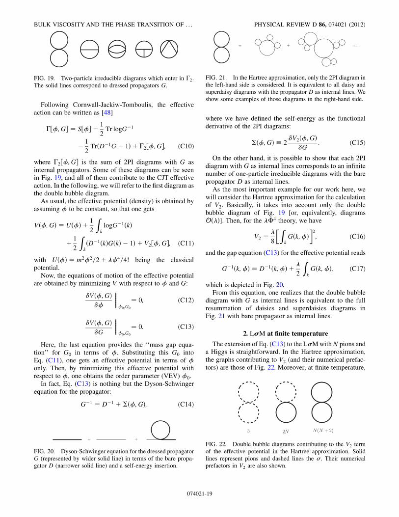
will consider the Hartree approximation for the calculationof V2. Basically, it takes into account only the doublebubble diagram of Fig. 19 [or, equivalently, diagramsOð�Þ]. Then, for the ��4 theory, we have
V2 ¼ �
8
�ZkGðk;�Þ
�2; (C16)
and the gap equation (C13) for the effective potential reads
G�1ðk;�Þ ¼ D�1ðk;�Þ þ �
2
ZkGðk;�Þ; (C17)
which is depicted in Fig. 20.From this equation, one realizes that the double bubble
diagram with G as internal lines is equivalent to the fullresummation of daisies and superdaisies diagrams inFig. 21 with bare propagator as internal lines.
2. L�M at finite temperature
The extension of Eq. (C13) to the L�MwithN pions anda Higgs is straightforward. In the Hartree approximation,the graphs contributing to V2 (and their numerical prefac-tors) are those of Fig. 22. Moreover, at finite temperature,
FIG. 19. Two-particle irreducible diagrams which enter in �2.The solid lines correspond to dressed propagators G.
FIG. 20. Dyson-Schwinger equation for the dressed propagatorG (represented by wider solid line) in terms of the bare propa-gator D (narrower solid line) and a self-energy insertion.
FIG. 22. Double bubble diagrams contributing to the V2 termof the effective potential in the Hartree approximation. Solidlines represent pions and dashed lines the �. Their numericalprefactors in V2 are also shown.
FIG. 21. In the Hartree approximation, only the 2PI diagram inthe left-hand side is considered. It is equivalent to all daisy andsuperdaisy diagrams with the propagator D as internal lines. Weshow some examples of those diagrams in the right-hand side.
BULK VISCOSITY AND THE PHASE TRANSITION OF . . . PHYSICAL REVIEW D 86, 074021 (2012)
074021-19

the k integration should be replaced by Matsubara summa-tions. Defining
Z�fði!n;kÞ ¼ T
Xn
Z d3k
ð2�Þ3 fði!n;kÞ; (C18)
where !n ¼ 2�Tn, the effective potential reads
Vð�;GÞ ¼ Uð�Þ þ 1
2
Z�logG�1
� ðkÞ
þ N
2
Z�logG�1
� ð�; kÞ
þ 1
2
Z�½D�1
� ðk;�ÞG�ð�; kÞ � 1Þ
þ N
2
Z�½D�1
� ðk;�ÞG�ð�; kÞ � 1Þ
þ V2ð�;G�;G�Þ; (C19)
where V2 is given by
V2ð�;G�;G�Þ ¼ 3�
N
�Z�G�ð�; kÞ
�2
þ NðN þ 2Þ �N
�Z�G�ð�; kÞ
�2
þ 2N�
N
Z�G�ð�; kÞ
Z�G�ð�; kÞ:
(C20)
The two gap equations are obtained by minimizing theeffective potential with respect to G� and G�:
G�1� ð�Þ ¼ D�1
� ð�Þ þ 4�Z�G�ð�Þ þ 12�
N
Z�G�ð�Þ;
(C21)
G�1� ð�Þ ¼ D�1
� ð�Þ þ 4ðN þ 2Þ�Z�G�ð�Þ
þ 4�
N
Z�G�ð�Þ: (C22)
To solve the system, one can use the ansatz for thedressed propagator: G�1
i ¼ k2 þM2i , with Mi being the
effective masses. Minimizing the effective potential (C19)with respect to �, one obtains the third equation whichcloses the nonlinear system leading to the three parameters� (eventually called v), M� and M�. Introducing theexplicit form of the bare and dressed propagators, theeffective potential finally reads
Vð�;MÞ ¼ � ��2�2 þ �
N�4 � ��þQðM�Þ þ NQðM�Þ
þ 1
2
��2 ��2 þ 12�
N�2 �M2
�
�FðM�Þ
� N
2
��2 ��2 þ 4�
N�2 �M2
�
�FðM�Þ
þ 3�
N½FðM�Þ�2 þ ðN þ 2Þ�½FðM�Þ�2
þ 2�FðM�ÞFðM�Þ; (C23)
where
FðMÞ ¼Z�
1
k2 þM2
¼Z d3k
ð2�Þ31
2Ek
þZ d3k
ð2�Þ31
Ek
1
e�Ek � 1; (C24)
and
QðMÞ ¼ 1
2
Z�logðk2 þM2Þ
¼Z d3k
ð2�Þ3Ek
2þ T
Z d3k
ð2�Þ3 log½1� e��Ek�; (C25)
with Ek ¼ffiffiffiffiffiffiffiffiffiffiffiffiffiffiffiffiffiffik2 þM2
p. As it is well known, both integrals
have a T ¼ 0 (divergent) and a finite temperature-dependent part. The renormalization of the effective po-tential is discussed in Ref. [44] and references therein. Inparticular, there exists some difficulties in the renormal-ization under the Hartree approximation. See Refs. [52,53]for more details [54]. To our purposes, we only take intoaccount the finite thermal contributions FðMÞ ! F�ðMÞand QðMÞ ! Q�ðMÞ.
[1] A. Adare et al. (PHENIX Collaboration), Phys. Rev. Lett.98, 162301 (2007).
[2] K. Aamodt et al. (ALICE Collaboration), Phys. Rev. Lett.105, 252302 (2010).
[3] M. Luzum and P. Romatschke, Phys. Rev. C 78, 034915(2008); 79, 039903(E) (2009).
[4] H. Song and U.W. Heinz, J. Phys. G 36, 064033 (2009).[5] P. Bozek, J. Phys. G 38, 124043 (2011).
[6] P. K. Kovtun, D. T. Son, and A.O. Starinets, Phys. Rev.Lett. 94, 111601 (2005).
[7] L. P. Csernai, J. I. Kapusta, and L.D. McLerran, Phys. Rev.Lett. 97, 152303 (2006).
[8] A. Dobado, F. J. Llanes-Estrada, and J.M. Torres-Rincon,Phys. Rev. D 79, 014002 (2009).
[9] A. Dobado, F. J. Llanes-Estrada, and J.M. Torres-Rincon,Phys. Rev. D 80, 114015 (2009).
ANTONIO DOBADO AND JUAN M. TORRES-RINCON PHYSICAL REVIEW D 86, 074021 (2012)
074021-20

[10] A. Dobado, F. J. Llanes-Estrada, and J.M. T. Rincon, AIPConf. Proc. 1031, 221 (2008).
[11] S. Weinberg, Astrophys. J. 168, 175 (1971).[12] V. Canuto and S. H. Hsieh, Nuovo Cimento Soc. Ital. Fis.
48B, 189 (1978).[13] P. B. Arnold, C. Dogan, and G.D. Moore, Phys. Rev. D 74,
085021 (2006).[14] D. Fernandez-Fraile and A.G. Nicola, Phys. Rev. Lett.
102, 121601 (2009).[15] A. Dobado, F. J. Llanes-Estrada, and J.M. Torres-Rincon,
Phys. Lett. B 702, 43 (2011).[16] J.M. Torres-Rincon, Prog. Part. Nucl. Phys. 67, 461
(2012).[17] A. Onuki Phys. Rev. E 55, 403 (1997).[18] H. B. Meyer, Phys. Rev. Lett. 100, 162001 (2008).[19] F. Karsch, D. Kharzeev, and K. Tuchin, Phys. Lett. B 663,
217 (2008).[20] K. Paech and S. Pratt, Phys. Rev. C 74, 014901
(2006).[21] D. Kharzeev and K. Tuchin, J. High Energy Phys. 09
(2008) 093.[22] B.-C. Li and M. Huang, Phys. Rev. D 80, 034023
(2009).[23] P. Chakraborty and J. I. Kapusta, Phys. Rev. C 83, 014906
(2011).[24] D. Fernandez-Fraile, Phys. Rev. D 83, 065001 (2011).[25] E. Nakano, V. Skokov, and B. Friman, Phys. Rev. D 85,
096007 (2012).[26] K. Dusling and T. Schafer, Phys. Rev. C 85, 044909
(2012).[27] With respect to the Lagrangian in Ref. [9], we explicitly
show the N dependence of the coupling constant. TheLagrangian shown there was in Minkowski space.
[28] E. J. Weinberg and A.-q. Wu, Phys. Rev. D 36, 2474(1987).
[29] J. Iliopoulos, C. Itzykson, and A. Martin, Rev. Mod. Phys.47, 165 (1975).
[30] M. T.M. van Kessel, arXiv:0810.1412.[31] J. Alexandre, V. Branchina, and J. Polonyi, Phys. Lett. B
445, 351 (1999).[32] A. Dobado and J. Morales, Phys. Rev. D 52, 2878
(1995).[33] G. Aarts and J.M.M. Resco, J. High Energy Phys. 02
(2004) 061.[34] S. Jeon, Phys. Rev. D 52, 3591 (1995).[35] E.M. Lifshitz and L. P. Pitaevskii, Physical Kinetics
(Landau and Lifshitz Course of Theoretical Physics)(Pergamon, Oxford, 1981), Vol. 10.
[36] However, the component of AðpÞ parallel to x is not fixedby the BUU equation. If needed, it can be fixed by theLandau-Lifschitz condition.
[37] The conformal value of the squared speed of sounddepends on the space-time dimensions D and reads
v2SjCFT ¼ 1
D� 1:
[38] If the speed of sound is a monotonically increasing func-tion with temperature, as the relativistic limit is v2
S ¼ 1,this value can only be reached at T ! 1.
[39] G. S. Denicol, T. Kodama, T. Koide, and P. Mota, Phys.Rev. C 80, 064901 (2009).
[40] A. Bazavov, T. Bhattacharya, M. Cheng, N. H. Christ, C.DeTar, S. Ejiri, S. Gottlieb, R. Gupta et al., Phys. Rev. D80, 014504 (2009).
[41] S. Borsanyi, G. Endrodi, Z. Fodor, A. Jakovac, S. D. Katz,S. Krieg, C. Ratti, and K.K. Szabo, J. High Energy Phys.11 (2010) 077.
[42] M. Laine and Y. Schroder, Phys. Rev. D 73, 085009(2006).
[43] P. Gerber and H. Leutwyler, Nucl. Phys. B321, 387(1989).
[44] N. Petropoulos, arXiv:0402136.[45] In the Hartree approximation, the � is not N-suppressed
anymore, and it should be included in the thermodynam-ical functions. However, given the similar results inRef. [23], we will assume that the pertinent changes areminimal, and we do not include this degree of freedom inorder to maintain the simplicity in the kinetic theoryformalism.
[46] A. Muronga, Phys. Rev. C 76, 014910 (2007).[47] J.M. Torres-Rincon, Ph.D. thesis, Universidad
Complutense de Madrid, Spain, 2012, arXiv:1205.0782.[48] J.M. Cornwall, R. Jackiw, and E. Tomboulis, Phys. Rev. D
10, 2428 (1974).[49] G. Amelino-Camelia and S.-Y. Pi, Phys. Rev. D 47, 2356
(1993).[50] G. Amelino-Camelia, Phys. Lett. B 407, 268 (1997).[51] J. T. Lenaghan and D.H. Rischke, J. Phys. G 26, 431
(2000).[52] J. Berges, S. Borsanyi, U. Reinosa, and J. Serreau, Ann.
Phys. (Berlin) 320, 344 (2005).[53] G. Fejos, A. Patkos, and Z. Szep, Nucl. Phys. A803, 115
(2008).[54] We thank the referee for bringing these references to our
attention.
BULK VISCOSITY AND THE PHASE TRANSITION OF . . . PHYSICAL REVIEW D 86, 074021 (2012)
074021-21