Embed Size (px)
Citation preview

Building Interest Rate Curves and SABRModel Calibration
by
Jeffrey Ted Johnattan Mbongo Nkounga
Thesis presented in partial fulfilment of the requirementsfor the degree of Master of Science in Mathematics in the
Faculty of Science at Stellenbosch University
Department of Mathematical Sciences,Mathematics Division,
University of Stellenbosch,Private Bag X1, Matieland 7602, South Africa.
Supervisor: Prof. Ronnie Becker
March 2015

Declaration
By submitting this thesis electronically, I declare that the entirety of the workcontained therein is my own, original work, that I am the sole author thereof(save to the extent explicitly otherwise stated), that reproduction and pub-lication thereof by Stellenbosch University will not infringe any third partyrights and that I have not previously in its entirety or in part submitted it forobtaining any qualification.
Signature: . . . . . . . . . . . . . . . . . . . . . . . . . . .J.T. J Mbongo Nkounga
November 27, 2014Date: . . . . . . . . . . . . . . . . . . . . . . . . . . . . . . .
Copyright © 2015 Stellenbosch University All rights reserved.
i
Stellenbosch University https://scholar.sun.ac.za

Abstract
In this thesis, we first review the traditional pre-credit crunch approach thatconsiders a single curve to consistently price all instruments. We review thetheoretical pricing framework and introduce pricing formulas for plain vanillainterest rate derivatives. We then review the curve construction methodolo-gies (bootstrapping and global methods) to build an interest rate curve usingthe instruments described previously as inputs. Second, we extend this workin the modern post-credit framework. Third, we review the calibration of theSABR model. Finally we present applications that use interest rate curves andSABR model: stripping implied volatilities, transforming the market observedsmile (given quotes for standard tenors) to non-standard tenors (or inversely)and calibrating the market volatility smile coherently with the new marketevidences.
Keywords: credit crunch/crisis, credit risk, counterparty risk, collateral,CSA, interest rates, negative rates, Libor, Euribor, Eonia, forward curve, dis-count curve, single-curve, multiple-curve, interest rate derivatives, Deposit,FRA, Futures, OIS, IRS, basis swap, interpolation, global methods, boot-strapping, caps, swaptions, volatility, SABR, calibration.
ii
Stellenbosch University https://scholar.sun.ac.za

Acknowledgements
First, I would like to express my sincere gratitude to my supervisor, Prof.Ronnie Becker, for his invaluable support, continuous guidance, meticuloussuggestions and astute criticism and corrections, and for his inexhaustible pa-tience throughout this thesis.
Second, I would like to extend my deepest appreciation to AIMS for thistremendous opportunity and for the financial support. I would also like to ex-tend my appreciation to ACQuFRR members for various scientific exchanges.
Third, I would like to express my thanks to Marco Bianchetti and to Dr.Jöerg Kienitz for answering many of my questions and for keeping me abreaston the scientific developments around my thesis’s topic. Furthermore, I amvery very thankful to Daniel J. Duffy and Andrea Germani for assisting me inC# codes, Tran, H. Nguyen andWeigardh, Anton for their assistance regardingMatlab codes, and to QuantLib (Open Source) community, especially LuigiBallabio, for their assistance as far as C++ coding is concerned.
Last but not the least, I would like to express my heartfelt thanks to myfamily, for their prayers, patience, love, encouragement, moral support andblessings. Your Jeffrey is progressing step by step. I would also like to extendmy indebtedness to those who are no longer with us on this earth.
How can we forget the Almighty God, the Father of our Lord Jesus Christin Heaven? We put our trust in You. We praise You, we are grateful, we thankYou, we love You.
I will be what people think or say about me, only if I believe it.
iii
Stellenbosch University https://scholar.sun.ac.za

Dedications
To my family, relatives and friends.A big group with big hearts and strong beliefs.
iv
Stellenbosch University https://scholar.sun.ac.za

Contents
Declaration i
Abstract ii
Acknowledgements iii
Dedications iv
Contents v
List of Figures vii
List of Tables viii
Nomenclature ix
1 Introduction 1
2 Single Curve 32.1 Introduction . . . . . . . . . . . . . . . . . . . . . . . . . . . . 32.2 Definitions and notation . . . . . . . . . . . . . . . . . . . . . 32.3 Single curve framework . . . . . . . . . . . . . . . . . . . . . . 82.4 Curve construction mechanism . . . . . . . . . . . . . . . . . . 142.5 Options caps, floors and swaptions . . . . . . . . . . . . . . . 232.6 Summary and conclusion . . . . . . . . . . . . . . . . . . . . . 26
3 Multi-Curves 273.1 Introduction . . . . . . . . . . . . . . . . . . . . . . . . . . . . 273.2 Pricing valuation after the credit crunch . . . . . . . . . . . . 283.3 Multi curve framework . . . . . . . . . . . . . . . . . . . . . . 313.4 Options caps, floors and swaptions . . . . . . . . . . . . . . . 423.5 Summary and conclusion . . . . . . . . . . . . . . . . . . . . . 43
4 The SABR Model 444.1 Introduction . . . . . . . . . . . . . . . . . . . . . . . . . . . . 444.2 The SABR Model: description . . . . . . . . . . . . . . . . . . 47
v
Stellenbosch University https://scholar.sun.ac.za

CONTENTS vi
4.3 Model dynamics . . . . . . . . . . . . . . . . . . . . . . . . . . 494.4 Refinement of the SABR model . . . . . . . . . . . . . . . . . 604.5 Calibration of the SABR model . . . . . . . . . . . . . . . . . 614.6 Summary and conclusion . . . . . . . . . . . . . . . . . . . . . 72
5 Interest rate curves and SABR calibration applications 735.1 Introduction . . . . . . . . . . . . . . . . . . . . . . . . . . . . 735.2 Swaption smile and SABR functional form . . . . . . . . . . . 745.3 Summary and conclusion . . . . . . . . . . . . . . . . . . . . . 76
6 Conclusion 77
Appendices 79
A Numéraire change 80
B Day Count Conventions 82
C Interpolation and LMA 83C.1 Linear interpolation . . . . . . . . . . . . . . . . . . . . . . . . 83C.2 Cubic splines . . . . . . . . . . . . . . . . . . . . . . . . . . . 84C.3 Levenberg-Marquardt algorithm . . . . . . . . . . . . . . . . . 86
D Data 88D.1 Interest rate data . . . . . . . . . . . . . . . . . . . . . . . . . 88D.2 Swedish market (swaption) data . . . . . . . . . . . . . . . . . 90
E Interest rate derivatives pricing formulas 93E.1 FRA . . . . . . . . . . . . . . . . . . . . . . . . . . . . . . . . 93E.2 Futures . . . . . . . . . . . . . . . . . . . . . . . . . . . . . . 94E.3 IRS . . . . . . . . . . . . . . . . . . . . . . . . . . . . . . . . . 95E.4 OIS . . . . . . . . . . . . . . . . . . . . . . . . . . . . . . . . . 96E.5 IRBS . . . . . . . . . . . . . . . . . . . . . . . . . . . . . . . . 98
F Analysis of the SABR Model 99F.1 Singular Perturbation theory . . . . . . . . . . . . . . . . . . . 99F.2 Scaling . . . . . . . . . . . . . . . . . . . . . . . . . . . . . . . 102F.3 Application of perturbation theory to SABR model . . . . . . 103
G Fourier transform 120
H Computer code 122H.1 SABR model . . . . . . . . . . . . . . . . . . . . . . . . . . . 122H.2 Yield curves via Quantlib . . . . . . . . . . . . . . . . . . . . 129
List of References 134
Stellenbosch University https://scholar.sun.ac.za

List of Figures
2.1 Interest Rate Swap cash flows . . . . . . . . . . . . . . . . . . . . 92.2 Interest rate swap between Companies A and B . . . . . . . . . . 102.3 3M-Forward curve up to 50 years . . . . . . . . . . . . . . . . . . 202.4 Top panel: 6M-Forward curve up to 60 years, bottom panel: Effect
of data on the forward single curve . . . . . . . . . . . . . . . . . 212.5 Effect of data on the forward single curve . . . . . . . . . . . . . . 22
3.1 3m Euribor-Eonia, Basis Swap between different tenor. . . . . . . 303.2 EONIA 3M-Forward curve up to 2 years . . . . . . . . . . . . . . 383.3 Top panel: EONIA 3M-Forward curve up to 30 years, bottom
panel: Euribor 6M-Forward curve up to 30 years . . . . . . . . . . 393.4 Top panel: Euribor Discount curve up to 30 years, bottom panel:
effect of data on the forward curve using different interpolation . 403.5 Top panel: effect of data on the forward curve using different in-
terpolation, bottom panel:comparing discount curve: Euribor vsEONIA . . . . . . . . . . . . . . . . . . . . . . . . . . . . . . . . 41
4.1 Call’s volatility smile . . . . . . . . . . . . . . . . . . . . . . . . . 444.2 Volatility smile from data in Table D.2. Red dots: market volatility. 454.3 Dynamics of the parameter β . . . . . . . . . . . . . . . . . . . . 534.4 Dynamics of the parameter ρ . . . . . . . . . . . . . . . . . . . . 544.5 Dynamics of the parameter ν . . . . . . . . . . . . . . . . . . . . 554.6 Dynamics of the parameter α . . . . . . . . . . . . . . . . . . . . 564.7 Volatility smile shifting f . . . . . . . . . . . . . . . . . . . . . . 574.8 Shifting f in the backbone for β = 0 . . . . . . . . . . . . . . . . 584.9 Shifting f in the backbone for β = 1 . . . . . . . . . . . . . . . . 594.10 5Y12Y Calibration with different beta using Methods 1 and 2 . . 634.11 1M5Y Calibration with different beta using Method 1 and 2 . . . 644.12 5Y12Y swaption calibration using Methods 1 and 2 . . . . . . . . 664.13 1M5Y swaption calibration using Method 1 and 2 . . . . . . . . . 674.14 1M4Y swaption calibration using Method 1 for β = 0.5 and 1 . . 694.15 20Y4Y swaption calibration using Method 1 for β = 0.5 and 1 . . 704.16 1M20Y and 20Y20Y swaption calibration using Method 1 for β = 0.5. 71
vii
Stellenbosch University https://scholar.sun.ac.za

List of Tables
2.1 Data selected from Appendix D (D.1) . . . . . . . . . . . . . . . . 17
4.1 Comparison of I0 term Hagan vs Berestycki . . . . . . . . . . 614.2 Method 1 estimated for different beta . . . . . . . . . . . . . . . . 614.3 Method 2 estimated for different beta . . . . . . . . . . . . . . . . 624.4 Different methods calibrated when beta is 0 . . . . . . . . . . . . 654.5 Different methods calibrated when beta is 0.5 . . . . . . . . . . . 654.6 Different methods calibrated when beta is 1 . . . . . . . . . . . . 654.7 Some swaptions calibrated with Method 1 . . . . . . . . . . . . . 68
D.1 EUR Deposit strip . . . . . . . . . . . . . . . . . . . . . . . . . . 88D.2 EUR FRA strips on Euribor 3M, Euribor 6M, and Euribor 12M. . 88D.3 Hull-White parameters values for Futures 3M convexity adjustment
as of 11 Dec. 2012. . . . . . . . . . . . . . . . . . . . . . . . . . . 89D.4 EUR Futures on Euribor 3M . . . . . . . . . . . . . . . . . . . . . 89D.5 EUR IRS on Euribor 6M . . . . . . . . . . . . . . . . . . . . . . . 89D.6 EUR IRS on Euribor 3M . . . . . . . . . . . . . . . . . . . . . . . 89D.7 EUR IRS on Euribor 1M . . . . . . . . . . . . . . . . . . . . . . . 90D.8 EUR OIS . . . . . . . . . . . . . . . . . . . . . . . . . . . . . . . 90D.9 EUR IRBS . . . . . . . . . . . . . . . . . . . . . . . . . . . . . . 90
viii
Stellenbosch University https://scholar.sun.ac.za

Nomenclature
Notation and Abreviationsω Event or outcomeΩ Sample space that consists of all possible outcomeF Event spaceP Probability measure(Ω,F ,P) Probability spaceσ σ-algebraT ∗ Maximum fixed time horizon for all market activitiesFtt∈[0,T ∗] Flow of information at time trt Interest rate at time tBt Bank Account at time tP (a, b) Zero Coupon Bond at time a for the maturity bL(a, b) Simply-compounded spot interest rate (Libor rate) at time a for
the maturity bδ(a, b) Time interval between time a and b (according to day convention)F (t, S, T ) Simply-compounded forward interest rateK Fixed rateN Notional amountf(a, b) Instantaneous forward interest rate at time a for the maturity bQB Measure under numéraire B.
QT Measure under numéraire P (t, .)ET Expectation under the T-forward measureEQB
[.∣∣∣Ft] Conditional expectation under the measure QB on the Ft σ-field
T Fixed leg scheduleS Floating leg scheduleSα,β(t) Forward Swap RateCs Yield curveFs(t;Tj−1, Tj) s-Forward interest rateCapt Cap price at time t
ix
Stellenbosch University https://scholar.sun.ac.za

NOMENCLATURE x
Φ(.) Standard Normal cumulative distribution functionFloort Floor price at time tS(t, k, n) ATM strikeσi Volatility of the Caplet/Flooret between time interval [Ti−1, Ti](a− b
)+max(a− b, 0)
CPy (t0) Discount yield CurveCFy (t0) y-Forward yield Curvery y-Interest rateBy(t) Bank Account under y-Interest ratedcz Corresponding day count convention for the zero coupon rateTy y Fixed leg scheduleLy,j Spot Libor rate fixed on the market at time Tj−1
FRAStd Standard Forward Rate AgreementDepo(Tj;Tj) Payoff of the lender in an interest rate DepositRDepoy (T F0 ;Tj) y-Simply-compounded Deposit interest rate
FRAMkt Market Forward Rate AgreementRFuty (t;T) y-Simply-compounded Future interest rate
CFuty (t;Tj−1) Convexity adjustment
Futures(t;T) Futures payoff at paymentIRSletfloat Float coupon payoff Interest Rate SwapIRSletfix Fixed coupon payoff Interest Rate SwapAc(t;S) Annuity Swap discounted with Pc(t, .)ROISon Equilibrium OIS rateCc(T0) OIS Yield Curve at time T0
SABR Stochastic Alpha Beta RhoCMS Constant Maturity Swapsse Sum Squared Errorβ Exponent for the forward rateα Initial varianceν Volatility of varianceρ Correlation between the two Wiener processesK Strike priceF Forward rate of a log-normal underlying with constantr Risk-free interest rateσB Black-Scholes constant volatilitytex Time to maturityσmktj Market volatilities
Stellenbosch University https://scholar.sun.ac.za

Chapter 1
Introduction
Before the 2007-2008 credit crunch, the single curve approach was predom-inantly in use for consistently pricing financial instruments. This approachhas received less interest in the current literature, perhaps this is because theframework has become obsolete nowadays. Nevertheless, we can refer to Duffyand Germani (2013, Chapter 15). A more detailed literature review can befound in Chapter 2.
In contrast, the multi-curve approach has received a lot of interest in therecent literature. In particular, we can find more information in Duffy andGermani (2013, Chapter 16), Ametrano and Bianchetti (2009), Ametrano andBianchetti (2013) and others (we refer to Chapter 3 for a more detailed liter-ature review).
The Black-Scholes model is based on the assumption of constant volatil-ity cannot incorporate the volatility smiles usually observed in the markets.Therefore, we must consider alternative stochastic volatility models such as theSABR model. The SABR model was first introduced by Hagan et al. (2002).This model has received a lot of attention in the recent literature. Differentauthors have contributed to its extension and to its improvement. We cancite the works of Oblój (2008) and others (we refer to Chapter 4 for a moredetailed literature review).
Problem statement and limitationsUsing the SABR model, Mercurio and Pallavicini (2006) proposed a very sim-ple procedure for stripping consistently implied volatilities and CMS adjust-ments from the market quotes of swaption smiles and CMS swap spreads.Their approach was done in the single-curve framework. We aim to proposean extension of their approach in the multi-curve framework, but we only dealwith a method for stripping consistently implied volatilities from the marketquotes of swaption smiles. This work is inspired mainly by Bianchetti andCarlicchi (2011) and Kienitz (2013).
1
Stellenbosch University https://scholar.sun.ac.za

CHAPTER 1. INTRODUCTION 2
To achieve this, we start by reviewing the traditional pre-credit crunchapproach that considers a single curve to consistently price all instruments. Wethen review the curve construction methodologies (bootstrapping and globalmethods) to build an interest rate curve. Then, we extend this work in themodern post-credit framework. Furthermore, we review the calibration of theSABR model and we highlight the procedure of the calibration after the crisis.
Thesis outlineThe thesis is organized as follows. Chapter 2 presents the methodologies (Boot-strapping and Best Fit) for constructing interest rate curves (discounting andforward yield curves), accompanied by their implementation. It reviews thefundamental pricing formulas for plain vanilla interest rate derivatives in theclassical framework with no collateral. Chapter 3 gives an overview of a num-ber of changes that have taken place in the financial markets since the creditcrunch of 2007. It introduces the use of multiple distinct curves to ensure mar-ket coherent estimation of discount factors and of forward rates with differentunderlying rate tenors. Chapter 4 reviews the calibration of the SABR modelfor different swaptions. It presents two different methods (with and withoutrefinement), and shows that the SABR model accurately captures the volatil-ity smiles in the markets. Moreover, this chapter reveals the complexity ofthe market after the credit crunch. Chapter 5 presents applications that useinterest rate curves and SABR model such as: stripping implied volatilities,transforming the market observed smile (given quotes for standard tenors) tonon-standard tenors (or inversely) and calibrating the market volatility smilecoherently with the new market evidences. Finally, the summary and conclu-sion of the thesis is presented in Chapter 6. The data used in this thesis canbe found in Appendix D, also a summary code and more details and proofs ofsome formulae presented can be found in Appendices A, B, C, E, F, G and H.
Stellenbosch University https://scholar.sun.ac.za
Chapter 2
Single Curve
2.1 IntroductionGenerally, to trade financial instruments, we need to discount a set of cashflows occurring in the future or to estimate spot rates, forward rates for finan-cial transactions taking place in the future. The best way to achieve all theseis to construct an interest rate curve. In the finance market, there are twoframeworks for interest rate curve, mainly: Single Curve and Multi or Multi-ple Curves. The Single Curve represents the traditional or pre-credit crunchapproach, which considers a unique curve for both forwarding and discounting.However, after the 2007-2008 credit crunch, a unique curve for both forward-ing and discounting is no longer consistent (we will discuss this in Chapter3). Consequently, new approaches have begun to rise and to be used and theSingle Curve framework was superseded by the Multi-Curve framework.
In this chapter, we will provide some basics definitions and necessary con-cepts that we need later to explain the mechanism of the construction of curves.We assume that there is no default risk in the interbank (default risk and in-consistency between different instruments are ignored in this chapter).
2.2 Definitions and notationLet (Ω,F ,P,Ft) be a filtered probability space describing the market, where:
• Ω is the sample space that consists of all possible outcome ω ∈ Ω.
• F is the event space. It is a σ-algebra consisting of subsets (events) ofthe sample space X ⊆ Ω.
• P is the probability measure on the sample Ω. For any event X ⊆ Ω,P(X) is the probability of X occurring.
3
Stellenbosch University https://scholar.sun.ac.za

CHAPTER 2. SINGLE CURVE 4
Let T ∗ be the maximum fixed time horizon for all market activities. Thefiltration Ftt∈[0,T ∗] (that consists of a family of increasing σ-algebras) repre-sents a flow of information at time t. We have:
• For any a < b < T ∗ we have Fa ⊆ Fb ⊆ FT ∗ ≡ F .
• F0 = ∅,Ω.
Definition 2.1. A term structure of interest rates is a set of interest ratessorted by time to maturity. The curve shows the relation between the (level of)interest rate (or cost of borrowing) and the time to maturity.
We can build several types of curves using rates of a different nature, forexample zero coupon yield curve, forward rates curve, instantaneous forwardcurve. Below we provide basic mathematics formulae to deal with these termstructures of interest rates.
Definition 2.2 (Bank Account). Let rt be a positive stochastic function oftime and which models the short term interest rate. At time t > 0, the valueof a bank account is defined by Bt. We assume that the evolution of the bankaccount satisfies the following differential and initial condition:
dBt = rtBtdt, B0 = 1. (2.2.1)
By simple integration, equation (2.2.1) gives
Bt = exp(∫ t
0rsds
)∀ t ∈ [0, T ∗]. (2.2.2)
Definition 2.3 (Zero-Coupon Bonds). A T-maturity zero-coupon bond alsocalled a pure discount bond or a T-bond, is a contract that guarantees its holderthe payment of one unit of currency at time T , with no intermediate payments.At time t 6 T , the contract value is P (t, T ). It follows that P (T, T ) = 1 forall T 6 T ∗.
Using formula (A.0.1), when the bank account Bt is taken as the numéraire(i.e. Nt = Bt), then QN = QB and S(t) = P (t, T ). It follows that
P (t, T )Bt
= EQB[
1BT
∣∣∣∣∣Ft]. (2.2.3)
From equation (2.2.3), we have
P (t, T ) = EQB[exp
(−∫ T
trudu
)∣∣∣∣∣Ft]∀ t ∈ [0, T ]. (2.2.4)
Stellenbosch University https://scholar.sun.ac.za

CHAPTER 2. SINGLE CURVE 5
Definition 2.4 (Simply-compounded spot interest rate). The simply-compoundspot interest rate L(t, T ) is the constant rate defined by
L(t, T ) = 1− P (t, T )δ(t, T )P (t, T ) (2.2.5)
where δ(t, T ) is the time interval between time t and T (accrual factor accordingto the day convention chosen1).
The notation L is motivated by the fact that the market Libor2 rates aresimply-compounded rates.
Justification
Equation (2.2.5) can be explained as follows: we note L(t, τ) the Libor rate attime t, of tenor τ 3. At time t, if one lends 1 at Libor, then at time t+ τ , onereceives back 1 + δL(t, t + τ)L(t, τ), where δL(t, t + τ) is the actual time (daycount convention) between times t and t+ τ .
To avoid arbitrage (ignoring credit issues), we must have[1 + δL(t, t+ τ)L(t, τ)
]P (t, t+ τ) = 1. (2.2.6)
Equation (2.2.5) follows from this last expression.
Definition 2.5 (The T-Forward measure). The forward martingale measure(or briefly, the T-Forward measure) QT , corresponding to the zero couponbond P (t, T ) maturing at time T is an equivalent probability measure to QB
on (Ω,FT ), and is defined via the Radon-Nikodým derivative given by
ηT = dQT
dQB= B−1
T
EQB [B−1T ]
= 1P (0, T )BT
= B0P (T, T )P (0, T )BT
, QB-a.s.. (2.2.7)
Proposition 2.6. The relative prices, for t 6 U < T , P (t, U)/P (t, T ) aremartingales under QT .
Forward RatesForward rates are characterized by three time instants: the current time tat which the rate is considered, the settlement date S and its maturity Twith t < S 6 T . Forward rates are interest rates applicable to a financialtransaction that will take place in the future. We can define a forward ratethrough a (prototypical) forward-rate agreement (FRA).
1we refer to Appendix B for more details2Libor is the abbreviation of London Interbank Offered Rate, it is the average interest
rate at which a group of bank in the London market lend money to one another and it isoffered in ten major currencies .
3The tenor of interest rate is its maturity period, the period from the point of investmentto the time that interest is paid.
Stellenbosch University https://scholar.sun.ac.za

CHAPTER 2. SINGLE CURVE 6
Definition 2.7 (FRA). A FRA is contract in which two counterparties agreeto exchange two streams of cash flows in the same currency and in which thenotional principal N remains constant over the life of the contract. In thecontract, one party pays an interest rate based on the spot rate L(S, T ) andreceives a fixed rate K.
Formally, at time T one receives Nδ(S, T )K units of currency and pays theamount Nδ(S, T )L(S, T ) (assuming the same day-count conventions for bothparties). The value of the contract at time T is therefore:
Nδ(S, T )[K − L(S, T )
].
Using equation (2.2.5), the value of the contract at time T can be writtenas
N
[δ(S, T )K − 1
P (S, T ) + 1].
The value of the contract at time t, using equation (A.0.2), is
P (t, T )EQT[N[δ(S, T )K − 1
P (S, T ) + 1]∣∣∣∣∣Ft
].
This leads to
P (t, T )N[δ(S, T )K + 1
]− P (t, T )NEQT
[1
P (S, T )
∣∣∣∣∣Ft].
Using the fact that 1 = P (S, S), we have
P (t, T )N[δ(S, T )K + 1
]− P (t, T )NEQT
[P (S, S)P (S, T )
∣∣∣∣∣Ft].
Using Proposition 2.6, P (S, S)/P (S, T ) are martingales under QT , thereforethe total value of the contract at time t is
FRA(t, S, T, δ(S, T ), N,K) = N[P (t, T )δ(S, T )K − P (t, S) + P (t, T )
]. (2.2.8)
There is one value of K that ensures that the value of the contract at time t is0. The resulting rate is called the simply-compounded forward rate and whichwe define below.
Definition 2.8 (Simply-compounded forward interest rate). At time t, thecurrent time or the date today, we fix two future points S and T such thatt < S 6 T , where S is called settlement date and T is called time to maturity,the simply-compounded forward interest rate F (t;T, S) for [S, T ] contracted attime t, is defined by:
F (t;S, T ) = 1δ(S, T )
(P (t, S)P (t, T ) − 1
). (2.2.9)
Stellenbosch University https://scholar.sun.ac.za

CHAPTER 2. SINGLE CURVE 7
Hence, using equation (2.2.8), the value of the FRA can be written as
FRA(t, S, T, δ(S, T ), N,K) = NP (t, T )δ(S, T )[K − F (t;S, T )
]. (2.2.10)
Definition 2.9 (Instantaneous forward interest rate). The instantaneous for-ward interest rate, f(t, T ), contracted at time t for the maturity T > t isdefined by
f(t, T ) = limS→T+
F (t;T, S) = −∂ lnP (t, T )∂T
. (2.2.11)
The last equality follows from assuming that δ(S, T ) = T − S, for smallT − S
limS→T+
F (t;T, S) =− limS→T+
1P (t, S)
P (t, T )− P (t, S)S − T
=− 1P (t, T )
∂P (t, T )∂T
=− ∂ lnP (t, T )∂T
.
We consider also the following proposition.
Proposition 2.10. A simply-compounded forward rate spanning a time inter-val ending in T is a martingale under the T -forward measure, i.e.
EQT[F (v;S, T )
∣∣∣∣∣Ft]
= F (t;S, T ), 0 6 t 6 v 6 S < T. (2.2.12)
In particular, the forward rate spanning the interval [S, T ] is the QT -expectationof the future simply-compounded spot rate at time S for the maturity T, i.e.
EQT[L(S, T )
∣∣∣∣∣Ft]
= F (t;S, T ), 0 6 t 6 S < T. (2.2.13)
Definition 2.11 (Swap). A swap contract is the exchange between two coun-terparties, with no notional amount exchanged, of cash-flows (interest rates,or currencies). The agreement defines the dates when the cash flows are to bepaid and the way in which they are to be calculated.
There are many types of swaps. Among them we can cite: Interest RateSwaps, Currency Swaps, Credit Swaps, Commodity Swaps. Later on, we willdiscuss some of them, such as: Interest Rate Swap (IRS), Overnight IndexedSwap (OIS), Interest Rate Basis Swap (IRBS).
In a swap, the individual future cash flows that are swapped are called legs(there are: fixed legs and floating legs) which are calculated over a notionalprincipal amount. In an interest rate swap for instance, usually there is onecounterparty which agrees to pay the fixed rate and the other one which agrees
Stellenbosch University https://scholar.sun.ac.za

CHAPTER 2. SINGLE CURVE 8
to pay the floating rate (Libor rate for example) over the period, or an adjustedLibor rate (we will assume this in what follows). The fixed or floating rate ismultiplied by a notional principal amount and an accrual factor given by theappropriate day count convention.
Definition 2.12 (Over-the-counter market). Over-the-counter (OTC) marketis a decentralized market, without a central physical location, where marketparticipants trade with one another through various communication modes suchas the telephone, email and proprietary electronic trading systems.
Definition 2.13 (Collateral). Collateral consists of providing an item as asecurity against the possibility of payment default by the counterparty in acontract.
Yield curves notationWe denote by Cy the yield curve defined in a form of continuous term structureor discount factors (or zero coupon bonds)
CPy (t0) = T −→ Py(t0, T ), T > t0,
or forward rates
CFy (t0) = T −→ Fy(t0;T, T + y), T > t0
with t0 being a reference date of the curves (e.g. settlement date, sport date,or today). The subscript or index y corresponds to tenor, i.e.
y ∈ OIS, 1M, 2M, 3M, 6M, 12M.
2.3 Single curve frameworkIn this section we introduce the curve construction mechanism to build aninterest rate curve. After having introduced the idea of the interest rate curve,we give a basic overview of the instruments used as inputs as well as the mainmethods used in curve building such as bootstrapping and global methods.
2.3.1 Market instruments selectionThere are different types of instruments that can be selected for constructing aninterest yield curve, and it is impossible to include all available instruments inthe market. Therefore it is important to make a very careful selection of theseelements and to minimize the mispricing level of the excluded instruments.In the selection, the priority is given to more liquid4 instruments such as:
4The features of the liquid asset are: rapidity to be sold, minimal loss of value, any timewithin the market hours.
Stellenbosch University https://scholar.sun.ac.za
CHAPTER 2. SINGLE CURVE 9
Deposits, Forward rate agreements, futures, swaps, etc. We describe thesemarket instruments in detail below.
2.3.1.1 Interest Rate Swaps (IRS)
Interest Rate Swaps are OTC contracts in which two counterparties agree toexchange interest rate cash flows, based on a specified notional amount from afixed rate to a floating rate (or vice versa) or from one floating rate to another.They are generally used to manage exposure to fluctuations in interest rates.
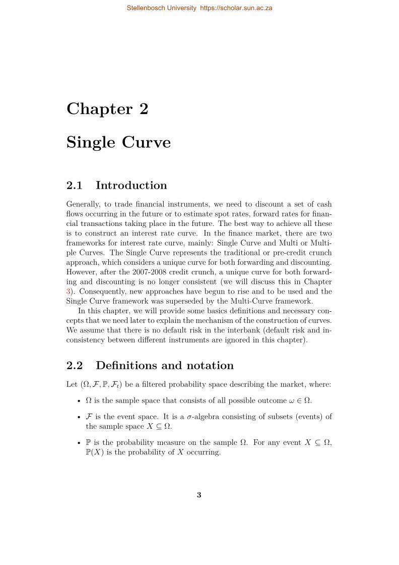
The illustration is given bellow on Figure 2.1, where the upward point-ing arrows are positive cash flows (fixed rate) and the downward pointingarrows are negative cash flows (floating rate). The gray arrows represent theexchanged amount for each period.
Figure 2.1: Interest Rate Swap cash flows. Blue arrows are cash flows(fixed rate) and red arrows are cash flows (floating rate), the gray arrowsare the exchanged amount.
Tables D.5, D.6, D.7, in this order, report the quoted swaps 1M, 3M, 6MEuribor rates. These cash flows are typically tied to a floating Libor rateL(Tj−1, Tj) versus a fixed rate K, therefore the IRS is characterised by thefollowing schedule
T = T0, T1, . . . , Tn, floating leg schedule,S = S0, S1, . . . , Sm, fixed leg schedule,S0 = T0, Sn = Tm.
Stellenbosch University https://scholar.sun.ac.za

CHAPTER 2. SINGLE CURVE 10
and coupon payoffs are
IRSletfloat(Tj;Tj−1, Tj, L) = NL(Tj−1, Tj)δL(Tj−1, Tj), j = 1, . . . , nIRSletfix(Si;Si−1, Si, K) = NKδK(Si−1, Si), i = 1 . . . ,m
(2.3.1)
where δK(Si−1, Si) is the fix leg time interval between Si−1 and Si and δL(Tj−1, Tj)is the floating leg time interval between Tj−1 and Tj. The coupon payoffs attime t, using equations (A.0.2) and (2.2.13), are given by
IRSletfloat(t, Tj;Tj−1, Tj, L) = NP (t;Tj)F (t;Tj−1, Tj)δL(Tj−1, Tj),IRSletfix(t, Si;Si−1, Si, K) = NKP (t;Si)δK(Si−1, Si).
The present value of the fixed leg, at time t, therefore is given by
PVfixed(t) = K ×N ×m∑i=1
P (t;Si)δK(Si−1, Si) (2.3.2)
and the present value of the floating leg, at time t, is given by
PVfloat(t) = N ×n∑j=1
P (t;Tj)F (t;Tj−1, Tj)δL(Tj−1, Tj). (2.3.3)
Using equation (2.2.9), the sum in equation (2.3.3) can then be simplified asfollows
n∑j=1
P (t;Tj)F (t;Tj−1, Tj)δL(Tj−1, Tj) = P (t;T0)− P (t;Tn). (2.3.4)
However, we will see in the next chapter, this will not be possible in themodern multiple-curve framework. Furthermore, because IRS are traded OTCcontracts; formula (A.0.3) will be used instead of formula (A.0.2).
Example 2.14. Company A and Company B want to borrow a certain amountof money each at the lowest possible cost for a certain period with annualcompounding. Company A expects interest rates to decline and wants floatingrate borrowing, while Company B expects interest rates to rise and wants tolock-in the fixed rate available to it.
Company A Company B
Fixed Rate: 6%
Floating Rate: LIBOR + 1%
Figure 2.2: Interest rate swap between Companies A and B
Stellenbosch University https://scholar.sun.ac.za

CHAPTER 2. SINGLE CURVE 11
Forward Swap RateThe forward swap rate Sα,β(t) at time t is the value of K that causes thecontract to have zero value at time t, i.e. such that PVfloat(t) = PVfixed(t), wehave:
Sα,β(t) = P (t, Sα)− P (t, Sβ)∑βj=α+1 δj,j−1P (t, Tj)
. (2.3.5)
2.3.1.2 Overnight Indexed Swap (OIS)
An Overnight Indexed swap (OIS) is an agreement between two counterpartiesto exchange at each payment date or at maturity the difference between fixedrate and floating rate on the nominal amount. The periodic floating rate isequal to the geometric average of an overnight rate over every day of the pay-ment period. For the EUR market the fixing is named EONIA (EUR OvernightIndex Average). The principal is not exchanged between counterparties at theend of the trade. The OIS coupon payoffs are given by
OISletfloat(Tj;Tj, Ron) = NRon(Tj;Tj)δon(Tj−1, Tj) j = 1, . . .m,OISletfix(Si;Si−1, Si, K) = IRSletfix(Si;Si−1, Si, K) i = 1, . . . n,
(2.3.6)
where Ron(Tj;Tj) is the coupon rate compounded from over night rates overthe j−th coupon period (Tj−1, Tj) and it is given by
Ron(Tj;Tj) := 1δ(Tj−1, Tj)
[ nj∏k=1
[1 +R(Tj,k−1, Tj,k)δ(Tj,k−1, Tj,k)]− 1]
where Tj = Tj,0, . . . , Tj,nj, is the sub-schedule for the coupon rate R(Tj,Tj),and R(Tj,k−1, Tj,k) are the single over night rate spanning the over night timeintervals (Tj,k−1, Tj,k). We have also Tj,0 = Tj−1, (Tj−1, Tj) = ⋃nj
k=1(Tj,k−1, Tj,k)and Tj,nj = Tj, for j = 1, . . . , n.
The price and equilibrium rate of the OIS is given, in Appendix E (equa-tions (E.4.9) and (E.4.10)), by
OIS(t;T, S, Rcon, K, ω) = Nω
[ROISon (t;T,S)−K
]Ac(t;S)
and
ROISx (t;T,S) =
∑mj=1 Pc(t;Tj)Ron(t;Tj)δon(Tj−1, Tj)
Ac(t;S)
= Pc(t;T0)− Pc(t;Tm)Ac(t;S) (2.3.7)
where
Ac(t;S) =n∑i=1
Pc(t;Si)δK(Si−1;Si). (2.3.8)
Stellenbosch University https://scholar.sun.ac.za

CHAPTER 2. SINGLE CURVE 12
In Table D.8, we have a report of the OIS on Eonia from 1W to 60Y whichstarts at T0 = today + 2 business and we notice very low and negative quota-tions for short term OIS.
Considering the OIS schedule Tj = T0, . . . , Tj = Sj, equation (2.3.7)gives
ROISon (T0;Ti−1) = Pc(t;T0)− Pc(t;Ti−1)
Ac(T0;Ti−1) .
From equation (2.3.8), we haveAc(T0;Ti) = Ac(T0;Ti−1) + Pc(T0;Ti)δK(Ti−1;Ti).
Using the expression of ROISon (T0;Ti), ROIS
on (T0;Ti−1) and Ac(T0;Ti−1) above,the discount curve CPc (T0) at time Ti is given by
Pc(T0;Ti) =
[ROISon (T0;Ti−1)−ROIS
on (T0;Ti)]Ac(T0;Ti)+Pc(T0;Ti−1)
1+ROISon (T0;Ti)δK(Ti−1;Ti) . (2.3.9)
Using equations (2.2.9) and (2.3.9), the forward curve CFc (T0) at time Ti isgiven by
Fc(T0;Ti−1, Ti) = 1δon(Ti−1;Ti)
Pc(T0;Ti)[
1+ROISon (T0;Ti)δK(Ti−1;Ti)
][ROISon (T0;Ti−1)−ROIS
on (T0;Ti)]Ac(T0;Ti−1)+Pc(T0;Ti−1)
− 1
.2.3.1.3 Deposits
Interest rate deposits (Depos) are standard money market zero coupon con-tracts. The lender pays the amount N to the borrower at time T0 and atmaturity Tj the borrower pays back to the lender the amount N plus theinterest accrued over the period [T0, Tj] at the simply compounded Depositrate RDepo
y (T F0 ;Tj), fixed at time T F0 ≤ T0. We have the contract scheduleT F0 , T0, Tj. For the lender, the payoff at maturity Tj is given by
Depo(Tj;Tj) = N[1 +RDepo
y (T F0 ;Tj)δL(T0;Tj)]. (2.3.10)
Since Deposits are not traded on OTC, using equation (A.0.2), the price ofthe payoff at time t, satisfying T F0 ≤ t ≤ Tj, is given by
Depo(t;Ti) = P (t;Tj)EQTjt
[Depo(Tj;Tj)
]
= NP (t;Tj)[1 +RDepo
y (T F0 ;Tj)δL(T0;Tj)]. (2.3.11)
Deposits rates are treated as Libor rates, so we have RDepoy (T F0 ;Tj) = L(T0, Tj).
Table D.1 shows data on Euro Deposit from 1 day up to 1 year. The discountcurve CPy (T0) at time Tj is obtained using the following relation
Py(T0, Tj) = 11 +RDepo
y (t0;Tj)δL(T0, Tj), T0 < Tj. (2.3.12)
Stellenbosch University https://scholar.sun.ac.za

CHAPTER 2. SINGLE CURVE 13
2.3.1.4 Futures
Futures contracts are agreements to buy or sell a stated amount of a security,currency, commodity, or a financial instrument, at a predetermined futuredate and price. While an option gives the holder the right to buy or sell theunderlying asset at expiration, the holder of the Futures contract is obligated tofulfil the terms of his or her contract. Before the crisis, Futures were treated asFRA (Definition 2.7). We will see the change in evaluating Futures in Section3.3.2.3.
2.3.1.5 Basis Swaps (IRBS)
Interest Rate Basis Swaps are OTC contacts in which two parties exchange twofloating rate (with different tenor x and y) payments in the same or differentcurrencies. This is usually done to limit interest-rate risk that a company facesas a result of having differing lending and borrowing rates.
There are two ways of building IRBS instruments: two fixed vs floatingIRS, and single IRS floating vs floating plus spread. We only treat the latterway (floating vs floating plus spread), because it is most used.
IRBS as single IRS
Here, the IRBS is a portfolio of a floating vs floating IRS with legs indexed totwo different Libors.
Tx = Tx,0, . . . , Tx,nx, x leg schedule,Ty = Ty,0, . . . , Ty,ny, y leg schedule,with Tx,0 = Ty,0, Tx,nx = Ty,ny
and coupon payoffs are
IRBSletx = NLx(Tx,i−1, Tx,i)δL(Tx,i−1, Tx,i)
IRBSlety = N[Ly(Ty,j−1, Ty,j) +4(t;Tx,Ty)]δL(Ty,j−1, Ty,j)
(2.3.13)
with i = 1, . . . , nx ; j = 1, . . . , ny; k = 1, . . .m and where 4(t;Tx,Ty)in the second leg is a constant basis spread on Ly(Ty,j−1, Ty,j) for maturityTx,nx = Tx,ny . The EUR market quotes standard plain vanilla Basis swapunder the form aM vs bM , it is a kind of swap where we have the same fixedlegs and floating legs paying Euribor aM and bM . Before the crisis, the basisspread 4(t;Tx,Ty) was negligible. Hence
IRBSletx ' IRBSlety.
Therefore, for instance, for a IRBS receiving Euribor yM and paying Euribor3M for maturity Tj, we have
RIRSx (t,T,S) ' RIRS
3M (t,T,S). (2.3.14)
Stellenbosch University https://scholar.sun.ac.za

CHAPTER 2. SINGLE CURVE 14
InterpolationInterpolation is a method of constructing new data points within the rangeof a discrete set of known data points. In other words, it is a process ofapproximating the value of a function y(t) (satisfying y(τj) = yj) between twopoints at which it has prescribed values.
Interpolation is very important in yield curve construction and determinessome characteristics of the curve. A lot of risk and money can be hidden behindthe interpolation method. There are many choices of interpolation function,however we are interested in interpolations that preserve arbitrage-free con-ditions, localness (a change in an input, affects the shape of the curve onlylocally), smoothness, positivity and stability (a change in an input, does notaffect the entire shape of the curve) of forward rates. A typical headache for aninterest rate trader is to choose between forward curve smoothness and bumphedge localness. Also we cannot use more than one method simultaneously(because each method satisfies specific requirement).
Interpolation, as we will see in Example 2.4.5, can be used in two phases.First, directly on market quotes to complete missing information. Second,internally to return discount factors for time intervals not directly coveredby information of interest rates (the interaction between these two phases iscrucial).
In Appendix C, we present the interpolation methods that are used in thiswork. More details about interpolation can be found in Hagan and West (2008)or Duffy and Germani (2013).
2.4 Curve construction mechanismThere are two main methods for curve construction starting from market data:traditional bootstrapping method and the global method. In both cases thecurve building process should be calibrated to a set of quotes by solving theequations that set the theoretical values equal to the market values. Also, inboth cases, we underline that interpolation is needed to complete missing datathrough the process of calibration.
2.4.1 Bootstrapping methodThe traditional bootstrapping method consists in solving the equations that setthe theoretical values equal to market values sequentially (Example 2.4.5). Weassume that different instruments are associated with different dates, so that,for instance, we cannot calibrate both on a 6m deposit and a 6m swap sincethey would be associated with the same calibration date. Starting from shortermaturities we progress sequentially to longer maturities. In the process missinginformation can be retrieved using interpolation. Because the process is done
Stellenbosch University https://scholar.sun.ac.za

CHAPTER 2. SINGLE CURVE 15
sequentially, for this reason only interpolation that preserves the localnessshould be used (for example, the linear on the logarithm of discount factorinterpolation method).
2.4.2 Best Fit methodCurve fitting is the process of constructing a curve that has the best fit to aseries of data points, possibly subject to constraints. Curve fitting can involveeither interpolation, where an exact fit to the data is required, or smoothing,in which a “smooth” function is constructed that approximately fits the data(for this end we may use Levenberg-Marquardt nonlinear least squares solveralgorithm).
2.4.3 Single curve market instruments selectionThe single curve was usually constructed based on the selection of the followingmarket instruments5 (more information can be found in common textbookssuch as: Hull (2009), Rebonato and Rebonato (1998), Chibane et al. (2009)).
1. Deposit contracts, covering the window from today up to 1Y.
2. FRA contracts, covering the window from 1M up to 2Y.
3. Futures contracts, covering the window from 3M up to 2Y and more.
4. IRS contracts, covering the window from 2Y-3Y up to 30Y.
The instruments cited above are not homogeneous in the underlying rate (theyadmit underlying interest rates with mixed tenors).
2.4.4 Single curve bootstrapping approachThe pre-crisis standard market practice, which was based on the single-curveapproach (and that can be found for instance in: Ron (2000), Ametranoand Bianchetti (2009), Bianchetti (2008), Hagan and West (2006), Ametrano(2011), Hagan and West (2008) and Andersen (2007)), can be summarised inthe following steps:
1. Interbank credit/liquidity issues do not matter for pricing, Libors aregood proxy for risk free rates, Basis Swap spreads are negligible (andnot taken into consideration).
2. The collateral does not matter for pricing, Libor discounting is adopted.5also called blocks
Stellenbosch University https://scholar.sun.ac.za

CHAPTER 2. SINGLE CURVE 16
3. Select one finite set of the most convenient vanilla instrument traded onthe market with increasing maturities.
4. Construct one yield curve by using the selected instruments (as in Section2.4.3).
5. Compute on the same curve FRA rates, discounts factors by using for-mulae presented in Section 2.3.1 above.
6. If necessary, compute the delta sensitivity and hedge the resulting deltarisk using the suggested amounts (hedge ratios) of the same set of vanil-las.
We emphasis that, in this framework, on a given currency, a unique yield curveis built and used to price any interest rate derivative. It goes the same way tosuppose that there exists a unique underlying short rate process that is ableto model and explain the whole term structure of interest rates for all tenors.In addition, the prices of a derivative are calculated relatively to a set of plainvanillas quoted on the market. Finally given the fact that discount factors andforward rates are obtained by interpolation, it follows in general that, theremay exist arbitrage possibilities.
General settings
The reference date for the yield curve can be: today, spot date6 or in principalany business day after today. The reference date of the EUR market, exceptON (OverNight i.e. between today and tomorrow) and TN (Tomorrow Nexti.e. between Tomorrow and Next day) Deposit contracts, is t0 = spot date.The vector of all the dates of the curve from the reference date up to anymaturity is called the Time grid or pillars or also knots. The parameter whichdefines the reference currency of the yield curve corresponding to the currencyof the instruments is called Calendar.
TARGET Business Day refers to a day on which the Trans-European Au-tomated Real-time Gross Settlement Express Transfer (TARGET) System, orany successor thereto, is operating credit or transfer instructions with respectof payments in Euro. Business Day Convention is a procedure used for ad-justing payment dates in response to days that are not TARGET BusinessDays. Following Business Day Convention is a procedure in which paymentdays that fall on a Holiday or Saturday or a Sunday roll forward to the nextTARGET Business Day. On the other hand Modified Following Business DayConvention is a procedure in which payment days that fall on a Holiday orSaturday or a Sunday roll forward to the next TARGET Business Day, unlessthat day falls in the next calendar month, in which case the payment day rollsbackward to the immediately preceding TARGET Business Day.
6 spot date of a transaction is the normal settlement day when the transaction is donetoday.
Stellenbosch University https://scholar.sun.ac.za

CHAPTER 2. SINGLE CURVE 17
2.4.5 Yield curve bootstrapping exampleWe present here an example of bootstrapping a yield curve from data market.We use the theory presented above in a more pragmatic manner. In Section2.4.3, we have seen how to select markets instruments. Using data in TablesD.1, D.2, D.4 and D.5, we select markets instruments that we report in Table2.1 below. In Section 2.4.4, we have presented the steps used in the bootstrap-ping method. The idea is to build up sequentially the yield curve from shortermaturities to longer maturities (15y in this example).
The spot date t0 is 13 December, 2012 (13/12/12). The chosen day-countconvention is the Actual/360, hence
δ(T, S) = actual number of days between T and S360 .
Deposit (%) FRA (%) Futures Swaps (%)SN 0.040 FRA 2× 5 0.141 18 Sep 13 99.8725 2y 0.3241w 0.070 FRA 4× 10 0.256 18 Dec 13 99.8425 3y 0.4241m 0.110 19 Mar 14 99.8025 4y 0.5762m 0.140 18 Jun 14 99.7425 5y 0.7623m 0.180 7y 1.1356m 0.320 10y 1.584
15y 2.037
Table 2.1: Data selected from Appendix D (D.1)
• The first column in Table 2.1 contains the Deposit rates for maturities
T1, . . . , T6 = 14/12/12, 20/12/12, 14/01/13, 13/02/13, 13/03/13, 13/06/13.
Therefore, we have 1, 7, 32, 62, 90 and 182 days to maturity, respectively.The discount factor, using equation (2.3.12), is
P (t0, Ti) = 11 + L(t0, Ti)δ(t0, Ti)
.
for i = 1, . . . , 6.
• The second column in Table 2.1 contains the FRA rates for maturities
V1, V2 = 13/05/13, 15/10/13.
Note that the FRA 2× 5 starts the 13/02/13 and matures the 13/05/13and the FRA 4 × 10 starts the 15/04/13 and matures the 15/10/13.
Stellenbosch University https://scholar.sun.ac.za

CHAPTER 2. SINGLE CURVE 18
Therefore, we have 89 and 184 days to maturity, respectively. Thenusing equation (2.2.9), we have
P (t0, 13/05/13) = P (t0, 13/02/13)1 + δ(13/02/13, 13/05/13)F (t0, 13/02/13, 13/05/13) .
P (t0, 13/02/13) = P (t0, T4) is known from the previous block. Similarly,we have
P (t0, 15/10/13) = P (t0, 15/04/13)1 + δ(15/04/13, 15/10/13)F (t0, 15/04/13, 15/10/13) .
Here, however, P (t0, 15/04/13) is unknown. This is where interpola-tion comes in. We can interpolate P (t0, 15/04/13) between P (t0, T5)and P (t0, T6) from the previous block.
• The futures are quoted as futures price (third column in Table 2.1). Forsettlement day Ui, we can find futures rate by using the relation
100(1− FF (t0;Ui, Ui+1))
where FF (t0;Ui, Ui+1) is the futures rate for period [Ui, Ui+1] prevailingat t0 , and
U1, . . . , U5 = 18/09/13, 18/12/13, 19/03/14, 18/06/14, 17/09/14
hence δ(Ui, Ui+1) = 91/360. We treat futures rates as if they were simpleFRA rates (previous block), that is, we set
F (t0;Ui, Ui+1) = FF (t0;Ui, Ui+1).
Then using equation (2.2.9), we have
P (t0, Ui+1) = P (t0, Ui)1 + δ(Ui, Ui+1)F (t0, Ui, Ui+1) .
By this formula, we are able to calculate the discount factor P (t0, Ui) fori = 2, 3, 4, 5. However, we need to calculate P (t0, U1) first. Once again,interpolation is needed. We can interpolate P (t0, U1) between P (t0, V1)and P (t0, V2) from the previous block.The linear interpolation of the discount factors is given by:
P (0, T ) = Tk − TTk − Tk−1
P (0, Tk−1) + T − Tk−1
Tk − Tk−1P (0, Tk),
for Tk−1 6 T 6 Tk. While the linear interpolation of the log discountfactors is:
logP (0, T ) = Tk − TTk − Tk−1
logP (0, Tk−1) + T − Tk−1
Tk − Tk−1logP (0, Tk),
for Tk−1 6 T 6 Tk.
Stellenbosch University https://scholar.sun.ac.za

CHAPTER 2. SINGLE CURVE 19
• The fourth column in Table 2.1 contains the swaps rates (semi-annual)for maturities
S1, . . . S30
=
13/06/13, 13/12/13, 13/06/14, 15/12/14, 15/06/1514/12/15, 13/06/16, 13/12/16, 13/06/17, 13/12/1713/06/18, 13/12/18, 13/06/19, 13/12/19, 15/06/2014/12/20, 14/06/21, 13/12/21, 13/06/22, 13/12/2213/06/23, 13/12/23, 13/06/24, 13/12/24, 13/06/2515/12/25, 15/06/26, 14/12/26, 14/06/27, 13/12/27
The swap rate at t0 with maturity Sn is given by
Rswap(t0, Sn) = P (t0, S0)− P (t0, Sn)∑ni=1 δ(Si, Si+1)P (t0, Si)
, (S0 := t0). (2.4.1)
From the data we have Rswap(t0, Si) for i = 4, 6, 8, 10, 14, 20, 30. Oncemore, we obtain P (t0, S1), P (t0, S2) (and henceRswap(t0, S1), Rswap(t0, S2))by interpolation using previous blocks. All remaining swap rates are ob-tained through interpolation. For maturity S3 for instance, using linearinterpolation, we have
Rswap(t0, S3) = 12(Rswap(t0, S2) +Rswap(t0, S4)
).
Using equation (2.4.1), we get
P (t0, Sn) = P (t0, S0)−Rswap(t0, Sn)∑n−1i=1 δ(Si−1, Si)P (t0, Si)
1 +Rswap(t0, Sn)δ(Sn−1, Sn) .
This last formula gives P (t0, Sn) recursively for n = 3, . . . , 30.
Once we have calculated all the discount factors P , we are able to calculate allthe forward rates F (by using equation (2.2.8)) as well. We can then plot, thenumerical results over time. The forward rate curve produced by this methodmay be in some case wobbly, this implies that there may be some problemswith the method.
Problems with the Bootstrapping Method
An approximation is used when treating futures as if they were FRAs. In factan adjustment, called the convexity adjustment, is required to convert Futuresprices to equivalent FRAs (as we will see in equation (3.3.14)).
Some interpolations are required for the missing data, these interpolationmethods produce characteristic problems with forward rates calculated fromthe curve. Also, because this bootstrapping method works up from rates ofnearer maturity to rates of further maturity, a slight change in a nearer matu-rity rate can cause variations or oscillations farther up the forward rate curve.
Stellenbosch University https://scholar.sun.ac.za

CHAPTER 2. SINGLE CURVE 20
A poor bootstrapping method produces a characteristic symptom of a saw-tooth structure in the forward rate curve. This can be seen at the transitionmaturities between different instruments and at knot points of an inappropri-ate scheme.
An alternative method is to use Best Fit Method that would estimate asmooth yield curve parametrically from the market rates.
2.4.6 ImplementationWe apply here the methodologies illustrated in the previous sections to theconcrete EUR market case found in (Ametrano and Bianchetti, 2009), (Ame-trano and Bianchetti, 2013). We only report the yield curves: CF3M and CF6M .The numerical results have been obtained using (Duffy and Germani, 2013,Chapter 15) and QuantLib framework7. The yield curves reported here arethe final result of a complex chain of choices. Many alternatives choices arepossible.
Figure 2.3: 3M-Forward curve up to 50 years. Red: Single Curve usingBest Fit with Simple Cubic interpolation on log of discount factor, black:Single Curve using Best Fit smoothing with Simple Cubic interpolation onlog of discount factor, blue: Single Curve using Bootstrapping with Linearinterpolation on log of discount factor.
7More details can be found in Appendix H.
Stellenbosch University https://scholar.sun.ac.za

CHAPTER 2. SINGLE CURVE 21
Figure 2.4: Top panel: 6M-Forward curve up to 60 years. Red: SingleCurve using Bootstrapping with Linear interpolation on log of discountfactor, blue: Single Curve using Best Fit smoothing with Simple Cubicinterpolation on log of discount factor. Bottom panel: effect of data onthe forward single curve. Red: Bootstrapping with Linear interpolation onlog of discount factor using more data, blue: Bootstrapping with Linearinterpolation on log of discount factor using less data.
Stellenbosch University https://scholar.sun.ac.za

CHAPTER 2. SINGLE CURVE 22
Figure 2.5: Top panel: effect of data on the forward single curve. Red:Best Fit with Linear interpolation on log of discount factor using moredata, blue: Best Fit with Linear interpolation on log of discount factor us-ing less data. Bottom panel: effect of data on the forward single curve.Red: Smoothing Forward with Simple Cubic interpolation on log of dis-count factor using more data, blue: Smoothing Forward with Simple Cubicinterpolation on log of discount factor using less data.
Stellenbosch University https://scholar.sun.ac.za

CHAPTER 2. SINGLE CURVE 23
Figure 2.3 is the 3M-Forward curve up to 50 years. Figure 2.4 (top panel)shows the 6M-Forward curve up to 60 years. “SCBootstrappingLinearOn-LogDf” stands for Single Curve using Bootstrapping methodology with Linearinterpolation on log of discount factor, “SCBestFitSimpleCubicOnLogDf”stands for Single Curve using Best Fit methodology with Simple Cubic inter-polation on log of discount factor (the curve is not necessarily smooth) and“SCSmoothingFwdSimpleCubicOnLogDf” stands for Single Curve usingBest Fit methodology with Simple Cubic interpolation on log of discount factor(the curve is required to be smooth on forward rate). The difference betweenthe two methodologies (Bootstrapping and Best Fit) and the impact of thechosen interpolation method can be seen from the figure. It can be seen fromthe figures that there is no much difference between yield curves CF3M and CF6M .
Figure 2.4 (bottom panel) and Figure 2.5 are the plots of 6M-Forwardcurve. “BestFitSimpleCubicInterpolatorOnLogDfMore” stands for BestFit methodology with Linear interpolation on log of discount factor using moredata, “BestFitSimpleCubicInterpolatorOnLogDfLess” stands for BestFit methodology with Linear interpolation on log of discount factor usingless data. “BootstrappingLinearOnLogDfMore” stands for Bootstrap-ping methodology with Linear interpolation on log of discount factor usingmore data, “BootstrappingLinearOnLogDfLess” stands for Bootstrap-ping methodology with Linear interpolation on log of discount factor usingless data. “SmoothingFwdSimpleCubicOnLogDfMore” stands for BestFit methodology with Simple Cubic interpolation on log of discount factorusing more data, “SmoothingFwdSimpleCubicOnLogDfLess” stands forBest Fit methodology with Simple Cubic interpolation on log of discount factorusing less data.
As expected, when market quotes are rare, there is a higher impact fromthe interpolation scheme on forward rates shape, also from the methodolo-gies. Other strategies allow us to mitigate the impact from the interpolationscheme, for instance we build the discount curve using linear interpolation onthe discount factors and we change interpolation for forward rates.
2.5 Options caps, floors and swaptionsWe introduce here options on caps, floors and swaptions, which are over-the-counter (OTC) contracts and known as plain-vanilla (or standard) interest-rateoptions.
Definition 2.15. A cap is an OTC contract by which the seller agrees topayoff a positive amount to the buyer of the contract if the reference rate exceedsa prespecified level called the exercise rate of the cap on given future dates. Theseller of a floor agrees to pay a positive amount to the buyer of the contractif the reference rate falls below the exercise rate on some future dates.
Stellenbosch University https://scholar.sun.ac.za
CHAPTER 2. SINGLE CURVE 24
We note some terms: the reference rate is an interest-rate index based,for example, on Libor, swap rates from which the contractual payments aredetermined; the exercise rate or strike rate is a fixed rate determined at theorigin of the contract; the settlement frequency refers to the frequency withwhich the reference rate is compared to the exercise rate; the starting date isthe date when the protection of caps and floors begins.
Let us consider a cap with a nominal amount N , an exercise rate K, basedupon an underlying rate L(Ti−1, Ti) which covers a period from Ti−1 to Tiand with the schedule T0, T1, . . . , Tn. T0 is the starting date of the cap andTn − T0 expressed in years is the maturity of the cap. On each date paymentTi, the cap holder receives a cash flow Ci, given by:
Ci = Nδ(Ti−1, Ti)(L(Ti−1, Ti)−K
)+. (2.5.1)
Ci is a call option on L(Ti−1, Ti) observed on date Ti−1 with a payoff occurringon date Ti. The cap is a portfolio of n such options. The n call options of thecap are known as the caplets.
The cap price at date t in the Black (1976) model is given by
Capt =n∑i=1
Capletit =n∑i=1
Nδ(Ti−1, Ti)P (t, Ti)[F (t;Ti−1, Ti)Φ(di)
−KΦ(di − σi√Ti−1 − t)
].
(2.5.2)
Where
di =log
(F (t;Ti−1,Ti)
K
)+ σ2
i (Ti−1−t)2
σi√Ti−1 − t
and where σi is the volatility of a caplet over[Ti−1, Ti
], and Φ is the standard
Normal cumulative distribution function.Let us now consider a floor with the same characteristics. The floor holder
gets on each date Ti
Fi = Nδ(Ti−1, Ti)(K − L(Ti−1, Ti)
)+. (2.5.3)
Fi is a put option on L(Ti−1, Ti) observed on date Ti−1 with a payoff occurringon date Ti. The floor is a portfolio of n such options. The n put options ofthe floor are known as the floorlets.
The floor price at date t in the Black (1976) model is given by
Floort =n∑i=1
Floorletit =n∑i=1
Nδ(Ti−1, Ti)P (t, Ti)[− F (t;Ti−1, Ti)Φ(−di)
+KΦ(−di + σi√Ti−1 − t)
].
(2.5.4)
Stellenbosch University https://scholar.sun.ac.za

CHAPTER 2. SINGLE CURVE 25
2.5.1 Cap and floor at the money strikeA cap or a floor is considered ATM (at the money) if the strike K is equal tothe forward swap rate calculated according to the cap or floor conventions. Attime Ti, we define φ by
φ(Ti) =n∑i=1
(Ci − Fi
).
Using equations (2.5.1) and (2.5.3), we have
φ(Ti) =n∑i=1
Nδ(Ti−1, Ti)(L(Ti−1, Ti)−K
).
Using equations (A.0.2) and (2.2.13), we have
φ(t, Ti) =n∑i=1
NP (t, Ti)δ(Ti−1, Ti)(F (t;Ti−1, Ti)−K
).
Hence,
Cap− Floor =n∑i=1
NP (t, Ti)δ(Ti−1, Ti)(F (t;Ti−1, Ti)−K
).
Therefore the ATM strike is given by
S =∑ni=1 δ(Ti−1, Ti)P (t, Ti)F (t;Ti−1, Ti)∑n
i=1 δ(Ti−1, Ti)P (t, Ti). (2.5.5)
In the single-curve framework, using equation (2.2.8), the ATM strike is givenby
S(t, k, n) = P (t, Tk)− P (t, Tn)∑ni=k+1 δ(Ti−1, Ti)P (t, Ti)
. (2.5.6)
Definition 2.16. A swaption is an option granting its owner the right butnot the obligation to enter into an underlying swap. Although options can betraded on a variety of swaps, the term “swaption” typically refers to optionson interest rate swaps.
There are two types of swaption contracts:
• A payer swaption gives the owner of the swaption the right to enter intoa swap where they pay the fixed leg and receive the floating leg.
• A receiver swaption gives the owner of the swaption the right to enterinto a swap in which they will receive the fixed leg, and pay the floatingleg.
Stellenbosch University https://scholar.sun.ac.za

CHAPTER 2. SINGLE CURVE 26
The Black formula for a payer and a receiver swaption are
Payer(t) =n∑
i=k+1Nδ(Ti−1, Ti)P (t, Ti)
[S(t, k, n)Φ(di)−KΦ(di − σi
√Ti−1 − t)
](2.5.7)
and
Receiver(t) =n∑
i=k+1Nδ(Ti−1, Ti)P (t, Ti)[
KΦ(−di + σi√Ti−1 − t)− S(t, k, n)Φ(−di)
](2.5.8)
where
di =log
(S(t,k,n)K
)+ σ2
i (Tk−t)2
σi√Tk − t
.
Finally, we define an at the money (ATM) payer or receiver swaption as aswaption having the strike K, as defined in formulae (2.5.7) and (2.5.8), equalto at the money swap as shown in formula (2.5.6).
2.6 Summary and conclusionIn this chapter we have described each market instrument used for the con-struction of an interest curve in the pre-crisis framework. We have illustratedmethodologies (Bootstrapping and Best Fit) for constructing both discountingand FRA yield curves, consistently with market instruments. We have pre-sented the implementation of both methodologies, we have focused on interestrate swap given that this instrument plays a relevant role in the curve buildingprocess. We have reviewed the fundamental pricing formulas for plain vanillainterest rate derivatives in the classical framework with no collateral.
Stellenbosch University https://scholar.sun.ac.za

Chapter 3
Multi-Curves
3.1 IntroductionThe credit crunch crisis of summer 2007 has revealed a large Basis Swap spread1 between single-currency interest rate instruments of different tenors, as a con-sequence just one single curve is not appropriate for market coherent estimationof forward rates of different tenors, such as 1, 3, 6, 12 months.
During the 2007 crisis it became clear that these no-arbitrage assumptions(equations (2.2.5), (2.2.6) and (2.2.9)) could break down due to counterparty2and liquidity risk3, for example. Moreover, it became more important to collat-eralise OTC deals in order to reduce the risk involved in bilateral transactions.The multi-curve framework was introduced precisely for the purpose of deal-ing with collateralised derivatives and with the new behaviour of the forwardrates. The traditional framework, using the same curve for discounting andfor estimating forward rates, was not flexible enough to capture these features;some “new” formulae are required.
In this chapter, we present current challenges about curve building acrossthe market. We stress that there is default risk in the interbank. Also, we usethe methodologies for building interest rate yield curves described in Chapter2 in the new framework.
The present of curvesMedia around February 2013 have revealed the problem of a “Libor Scandal”(also called “the crime of the century”), which was a revelation of the dis-honest practices connected to the Libor. Consequently, the Libor has lost itscredibility for being considered as a true proxy for borrowing costs or for fund-
1We refer to 2.3.1.5 for more details.2Counterparty risk refers to the risk that the other party in an agreement will default.3Liquidity risk is the risk that a given security or asset cannot be traded quickly enough
in the market to prevent a loss (or make the required profit).
27
Stellenbosch University https://scholar.sun.ac.za

CHAPTER 3. MULTI-CURVES 28
ing costs. The banks members were falsely inflating or deflating their ratesin order to profit from trades, or to give the impression that they were morecreditworthy than they were.
Following the credit crisis 2007-2008, new counterparty risk mitigationtechniques based on collateral agreements are widely used (even before therevelation of the “Libor Scandal”). The appropriate rate at which cash flowsshould be discounted when valuing a collateralized trade is the rate at whichcollateral earns interest.
3.2 Pricing valuation after the credit crunchWe highlight some reasons that have led to the requirement for a new pricingframework for interest rates derivatives valuation.
3.2.1 Impact of collateralisationStandard derivatives pricing theory relies on the assumption that one canborrow and lend at a unique risk-free rate. However, the situation is ratherdifferent these days; as a consequence of the 2007-2008 global financial crisis,historically stable relationships between government rates, Libor rates, etc,have broken down.
In order to mitigate credit risk among dealers, agreements (based on the so-called credit support annex (CSA) to the International Swaps and DerivativesAssociation (ISDA) master agreement) have been put in place to collateralisemutual exposures. Therefore Collateral could then be thought of as an essen-tially risk-free investment. The rate on collateral (such as the fed funds ratefor dollar transactions, Eonia for Euro, etc) is usually set to be a proxy of arisk-free rate. In addition, the pricing of non-collateralised derivatives needsto be adjusted accordingly, as compared to the collateralised version.
• The first adjustment is to use different discounting rates for CSA andnon-CSA versions of the same derivative.
• The second adjustment is a convexity, or quanto, adjustment and affectsforward curves as they turn out to depend on collateralisation used.
• The third adjustment that may be required is to volatility informationused for options, in particular, the volatility smile changes depending oncollateral.
We denote the short rate at time t by rc(t); c here stands for CSA, as we assumethis is the agreed overnight rate paid on the safest available collateral (cash)among dealers under CSA. The corresponding discount factor is Pc(t, T ).
Stellenbosch University https://scholar.sun.ac.za

CHAPTER 3. MULTI-CURVES 29
3.2.2 OIS discountingAn Overnight Indexed Swap (OIS) is a fixed/floating interest rate swap. Thefloating leg is tied to a published overnight rate index (EONIA). The counter-parties agree to exchange (at the repayment date) the difference between theagreed fixed rate and the interest accrued from the geometric average of thedaily floating overnight index rate over the time period based on the agreednotional amount.
OISs popularity have increased since the 2007/2008 financial crisis for manyreasons: they are liquid and credit-efficient derivatives for all major currencies,Libor-based instruments often failed to capture movements in policy rates, theycan be used to hedge against moves in overnight interest rates.
Collateralisation impacts the price of a derivative instrument and this is oneof the reason why the multicurve framework is needed. Consider, for example,a swap exchanging a fixed rate against a Libor rate. Before the crisis, the cashflows were discounted using the discount factors derived from the Libor swapcurve. However under collateralisation, the curve for discounting cash flows ofa swap should depend on how the swap is collateralised or funded. In a caseof bilateral contract with a poorly rated counterparty, we have an impact ofthe counterparty risk on the valuation of the derivative. Therefore it is notcorrect to use OIS discounting.
3.2.3 BasisAs it can be seen on Figure 3.1, before the financial crisis the 3m Euribor-OISspread had an average value of 8 basis points (average from May 2000 to July2007). So there was not a significant difference in pricing swap discounting withthe Euribor curve rather than the OIS curve. From August 2007 to August2008 the average spread was about 66 basis points. The crisis introduced awidening of the Euribor-OIS spread as a consequence of deteriorating bankcredit quality and fear of uncertainty.
Stellenbosch University https://scholar.sun.ac.za

CHAPTER 3. MULTI-CURVES 30
Figure 3.1: 3m Euribor-Eonia, Basis Swap between different tenor.
Stellenbosch University https://scholar.sun.ac.za

CHAPTER 3. MULTI-CURVES 31
3.3 Multi curve frameworkGiven the notation described above (Chapter 2), below we describe the evolu-tion of the financial market.
3.3.1 Multi curve market instruments selectionMulti Curves are usually constructed based on the selection of the followingmarket instruments4 (this way of selecting market instruments can be foundin common textbooks such as: Hull (2009), Rebonato and Rebonato (1998))
1. Deposit contracts, covering the window from today up to 1Y.
2. FRA contracts, covering the window from 1M up to 2Y.
3. Futures contracts, covering the window from 3M up to 2Y and more.
4. IRS contracts, covering the window from 2Y-3Y up to 30Y.
5. IRBS contracts, covering the window up to 60Y.
In contrast to Section 2.4.3, here the instruments are not homogeneous inthe underlying rate (they do not admit underlying interest rates with mixedtenors). We also note the presence of IRBS contracts.
3.3.2 The multi-curve approachSome of the weaknesses of the single curve approach presented in Chapter 2are:
• The basis swap spread can no longer be neglected due to the crisis (aspointed out in Section 3.2.3 above).
• As a consequence of the credit crunch, mixing different underlying ratetenors is no longer possible.
• Libor discounting was used5.
In order to remedy these weaknesses, the market has adopted a new frameworkwhich the summary of the procedure is given in the following steps:
1. Interbank/liquidity issues do matter for pricing, Libors risky rates, BasisSwap spreads are no longer negligible (and taken into consideration).
2. The collateral does matter for pricing, OIS discounting is adopted (Sec-tion 3.2.2).
4also called blocks5This is important to avoid arbitrage opportunities.
Stellenbosch University https://scholar.sun.ac.za

CHAPTER 3. MULTI-CURVES 32
3. Decide the appropriate discounting rate of derivatives to be priced, thenselect the corresponding market instruments and build one single dis-counting curve Cd using the classical single-curve methodologies de-scribed in Chapter 2.
4. Select multiple separated sets of vanilla interest rate instruments tradedon the market with increasing maturities, each set of homogeneous inthe underlying rate (e.g. 1M, 2M, 3M, 6M , 12M tenors).
5. Buildmultiple distinct forward curves C1M , C3M , C6M , C12M using theselected sets of vanilla interest rate market instruments plus their boot-strapping rules6 and the unique discount curve Cd.
6. If necessary, compute the delta sensitivity7 with respect to the marketpillars of each yield curve Cd, C1M , C3M , C6M , C12M and hedge the result-ing delta risk using the suggested amounts (hedge ratios) of the corre-sponding set of vanillas.
We note that, this new approach has been introduced to remedy the impactof the credit crisis as far as curve building is concerned, however practitionersshould be aware of some technical challenges such as:
• It can be inferred form the procedure of multiple curve building that thechoice of the discounting curve is crucial, consequently, this should bedone with more care.
• Multiples curves require many quotations available on the market suchas: Deposits, Futures, Swaps, Basis Swaps, FRA (we need data for eachtenor).
• Some interpolation methods may not produced smooth forward curves.
• All the theory about curve building must be reviewed, tested and (insome case) may be adapted to the new markets realities. This is not aneasy task for practitioners.
3.3.2.1 Interest Rates
Let Ly(Tj−1, Tj) := Ly,j be the spot Libor rate fixed on the market at timeTj−1 and spanning the interval [Tj−1, Tj] where y is the rate tenor. These ratesare mostly “risky” since they are traded with unsecured financial transactions.Depending on the type of transaction, tenor and possible collateral, the degreeof risk may be small or significant. Forward Libor rates are quoted in the
6Rules such as using the most liquid instruments, avoiding selecting instruments withsame maturities and so on.
7We do not present this point in this work.
Stellenbosch University https://scholar.sun.ac.za

CHAPTER 3. MULTI-CURVES 33
OTC derivatives market in terms of equilibrium rates of FRA (Forward RateAgreement) contracts. For simplicity we assume that both Libor and fixedrates have the simply compounded annual convention and they share the sameyear fraction δL. Based on the discussion given in Definition 2.7, the standardFRA payoff at cash flow date Tj is given by
FRAStd(Tj;T, Ly,j, K, ω) = ωN[Ly(Tj−1, Tj)−K
]δL(Tj−1, Tj). (3.3.1)
The FRA contract given in equation (3.3.1) is called “standard” or “textbook”FRA and differs from the “market” FRA quoted in the market (it is developedin Section 3.3.2.2). Since FRA are traded on OTC, using equation (A.0.3),the price of the payoff at time t is given by
FRAStd(t;T, Ly,j, K, ω) = Pc(t;Tj)EQTjc
t
[FRAStd(Tj;T, Ly,j, K, ω)
]
= ωNPc(t;Tj)EQ
Tjc
t
[Ly(Tj−1, Tj)
]−K
δL(Tj−1, Tj)
= ωNPc(t;Tj)[Fy,j(t)−K
]δL(Tj−1, Tj) (3.3.2)
where
Fy,j(t) := EQTjc
t
[Ly(Tj−1, Tj)
]. (3.3.3)
The FRA contact equilibrium rate is the value of the fixed rate K which is asolution of the equation
FRAStd(t;T, Ly,j, K, ω) = 0.
We get
K =: RFRAy,Std(t, Tj−1, Tj) = Fy,j(t) = EQ
Tjc
t
[Ly(Tj−1, Tj)
]. (3.3.4)
3.3.2.2 Forward Rate Agreements (FRAs)
Forward Rate Agreements are OTC contracts between parties that determinethe rate of interest, or the currency exchange rate, to be paid or received onan obligation starting at some point (date) in the future.
The actual FRA traded on the market, has a different payoff, such that, atpayment date Tj−1 (not Tj), we have
FRAMkt(Tj−1;T, Lx,j, K, ω) = Nω[Lx(Tj−1, Tj)−K)]δF (Tj−1, Tj)
1 + Lx(Tj−1, Tj)δF (Tj−1, Tj)
= FRAStd(Tj;T, Lx, K, ω)1 + Lx(Tj−1, Tj)δF (Tj−1, Tj)
. (3.3.5)
Stellenbosch University https://scholar.sun.ac.za

CHAPTER 3. MULTI-CURVES 34
Since FRAs are traded OTC between collateralized counterparties, we may ap-ply the pricing under collateral approach using equation (A.0.3). The price andthe equilibrium rate, derived in Appendix E (equations (E.1.4) and (E.1.5)),are given by
FRAMkt(t;T, K) = NPc(t;Tj−1)1− 1+Kδx(Tj−1,Tj)
1+Fx,j(t)δx(Tj−1,Tj)eCFRAc,x (t;Tj−1)
(3.3.6)
and
RFRAx,Mkt(t,T) = 1
δx(Tj−1,Tj)
[1 + Fx,j(t)δx(Tj−1, Tj)
]e−CFRAc,x (t;Tj−1) − 1
, (3.3.7)
where eCFRAc,x (t;Tj−1) is the convexity adjustment, depending on the particularmodel adopted for the dynamics of the rates Fd,j(t) and Fx,j(t).
The actual size of the convexity adjustment, even for long maturities, isbelow 1 bp (more details can be found in (Mercurio, 2010)). It follows that, inany practical situation, we can neglect the convexity adjustment and use theclassical pricing expressions, hence
FRAMkt(t;T, Lx,j, K, ω) ' FRAStd(t;T, Lx,j, K, ω).
It follows that
FRAMkt(t;T, Lx,j, K, ω) ' ωNPc(t;Tj)[Fx,j(t)−K
]δL(Tj−1, Tj) (3.3.8)
and
RFRAx,Mkt(t,T) ' RFRA
x,Std(t, Tj−1, Tj) = Fx,j(t) = EQTjc
t
[Lx(Tj−1, Tj)
]. (3.3.9)
FRAs are presented in the form a× b FRA which mean: a Effective date fromnow, b termination date from now, and b − a months Deposits. From TableD.2, for instance the 2× 8 FRA starts at T = 2 months and matures at T = 8months, it is a six months (6M) Deposit starting two months forward. Wenote that, the FRA dates concatenate exactly: the 2 × 8 FRA matures atT = 6M where the following 8× 14 starts.
Market FRAs provide direct empirical evidence that a single curve cannotbe used to estimate forward rates with different tenors. In the Table D.2 forinstance, we can see that the level of the market 2×5 FRA3M (spanning form13th February to 13th May, δL(2 × 5) = 0.24722) was RFRA
3M,Mkt(t0, 2 × 5) =0.141%, the level of the market 5 × 8 FRA3M (spanning form 13th May to13th August, δL(5 × 8) = 0.25555) was RFRA
3M,Mkt(t0, 5 × 8) = 0.124%. Bycompounding these two rates, the level of the implied 2×8 FRA6M (spanningform 13th February to 13th August, δL(2× 8) = 0.50278) would be
1 +RFRA6M,Implied(t0, 2× 8)δL(2× 8) =
[1 +RFRA
3M,Mkt(t0, 2× 5)δL(2× 5)][
1 +RFRA3M,Mkt(t0, 5× 8)δL(5× 8)
].
Stellenbosch University https://scholar.sun.ac.za

CHAPTER 3. MULTI-CURVES 35
It follows that
RFRA6M,Implied(t0, 2× 8) =
[1+RFRA
3M,Mkt(t0,2×5)δL(2×5)
][1+RFRA
3M,Mkt(t0,5×8)δL(5×8)
]−1
δL(2×8) .
Hence
RFRA6M,Implied(t0, 2× 8) = 0.1324%.
However, the market quote for 2×8 FRA6M was RFRA6M,Mkt(t0, 2×8) = 0.272%,
about 13.96 basis point larger.The discount factor at time Tj is given by
Py(T0, Tj) = Py(T0, Tj−1)1 +RFRA
y,Mkt(t0;Tj)δL(Tj−1, Tj). (3.3.10)
It can be seen that
limTj−1→T0
RFRAy,Mkt(t;Tj) = RDepo
y (t0, Tj). (3.3.11)
3.3.2.3 Futures
Futures were introduced in Chapter 2, Section 2.3.1.4. Interest Rate Futuresare equivalent to the OTC FRAs. The Futures payoff at payment date Tj−1 isgiven, from a point of view of the counterparty paying the floating rate, by
Futures(Tj−1;T) = N
[1− Ly(Tj−1, Tj)
]. (3.3.12)
The Futures rate at time t < Tj−1, derived in Appendix E (equations (E.2.2)and (E.2.3)), are given by
Futures(t;T) = NPc(t;Ti−1)
1−EQTict
[(1+Lc(Ti−1,Ti)δc(Ti−1,Ti)
)Ly(Ti−1,Ti)
]1+Fc,i(t)δc(Ti−1,Ti)
(3.3.13)
and
RFuty (t;T) = Fy,j(t) + CFut
y (t;Tj−1) (3.3.14)
where RFuty (t;T) is the rate implied by Futures price and its corresponding
FRA rate is Fy,j(t).A specific model is needed to compute the convexity adjustment to find
the Futures rate. For instance the mean reversion and the Volatility of theHull & White model were 3% and 0.3526% respectively for Futures3M at 11
Stellenbosch University https://scholar.sun.ac.za

CHAPTER 3. MULTI-CURVES 36
Dec. 2012. It can be seen, on Table D.4, that futures are quoted in terms ofprices instead of rates. We have the following relation
Futures(t;T) = 100×[1−RFut
y (t;T)]. (3.3.15)
Using equations (2.2.9) and (3.3.14), the discount curve CPy (t0) at time Tj isgiven by
Py(T0, Tj) = Py(T0, Tj−1)1 +
[RFuty (t0;Tj)− CFut
y (t0;Tj)]δL(Tj, Tj)
. (3.3.16)
If Cy(Tj−1) is known, the expression above can be used to bootstrap Cy(Tj).
3.3.2.4 Interest Rate Swaps (IRS)
IRS are traded OTC between collateralized counterparties, we may use theformula in equation (A.0.3). The IRS price, rate and annuity, derived inAppendix E (equations (E.3.5), (E.3.6) and (E.3.7)), are given by
IRS(t;T, S, Ly, K, ω) = Nω[RIRSy (t;T,S)−K
]Ac(t;S),
RIRSy (t;T,S) =
∑mj=1 Pc(t;Tj)Fy,j(t)δL(Tj−1, Tj)
Ac(t;S) (3.3.17)
and
Ac(t;S) =n∑i=1
Pc(t;Si)δK(Si−1, Si). (3.3.18)
We underscore that the classical telescopic property (as in equation (2.3.4)),such that
m∑j=1
Pc(t;Tj)Fx,j(t)δL(Tj−1, Tj) = Pc(t;T0)− Pc(t;Tm) (3.3.19)
does not hold any longer, because in the modern multiple-curve framework thediscount rate Pc and the forward rate Fx,j belong to two different yield curves.
From equation (3.3.17), the forward swap rate Sα,β(t) at time t is given by
Sα,β(t) =∑jβ=1 Pc(t;Tβ)Fy,β(t)δL(Tβ−1, Tβ)∑β
j=α+1 Pc(t;Sj)δK(Sj−1, Sj). (3.3.20)
From equation (3.3.17) the forward curve CFy (T0) at time Tj = Si is given by
Fy,j(T0) = RIRSy (T0;Tj)Ac(T0;Tj)−
∑j−1β=1 Pc(T0;Tβ)Fy,β(T0)δL(Tβ−1,Tβ)
Pc(T0;Tj)δL(Tj−1,Tj) . (3.3.21)
Stellenbosch University https://scholar.sun.ac.za

CHAPTER 3. MULTI-CURVES 37
Using equation (2.2.9), we have
Py(T0;Tj−1)Py(T0;Tj)
= 1 + Fy,j(T0)δL(Tj−1;Tj).
Using equation (3.3.21) above, we get
Py(T0;Tj−1)Py(T0;Tj) = 1 + RIRS
y (T0;Tj)Ac(T0;Tj)−∑j−1
β=1 Pc(T0;Tβ)Fy,β(T0)δL(Tβ−1,Tβ)Pc(T0;Tj) .
Hence
Py(T0;Tj) = Pc(T0;Tj)Py(T0;Tj−1)Pc(T0;Tj)+RIRS
y (T0;Tj)Ac(T0;Tj)−∑j−1
β=1 Pc(T0;Tβ)Fy,β(T0)δL(Tβ−1,Tβ). (3.3.22)
The equations (3.3.21) and (3.3.22) can be used to bootstrap the yield curveCy at point Tj = Si if we already know the curve at points T = T1, . . . , Tj−1and S = S1, . . . , Si−1. Some points between Py(t0, Tj−1) and Py(t0, Tj) inequation (3.3.22) can be unknown; we use interpolation for this end.
As an example, the bootstrap of Euribor6M curve C6M from 19Y to 20Yknots, we have RIRS
6M (T0, T20) = 2.187% in Table D.5, is given by
F6M,20Y (T0) = RIRS6M (20Y )Ac(20Y )−
∑j−1β=1 Pc(T0;Tβ)Fy,β(T0)δL(Tβ−1,Tβ)
Pc(20Y )δL(Tj−1,Tj) (3.3.23)
and
P6M(T20Y ) = Pc(20Y )P6M (19.5Y )Pc(20Y )+RIRS
6M (20Y )Ac(20Y )−∑j−1
β=1 Pc(T0;Tβ)Fy,β(T0)δL(Tβ−1,Tβ). (3.3.24)
Euribor6M being semi-annual, so T20 correspond to S40, so we have T =T1, . . . , T20, S = S1, . . . , S40, T19 = S38 = 19Y , S39 = 19.5Y , T20 = S40 =20Y . We have to interpolate P6M(S39) (unknown) in equation (3.3.24). We cansee (as we have seen in Section 2.4.5), the bootstrapping procedure containsthe interpolation.
3.3.2.5 Basis Swaps (IRBS)
Coupon payoffs were already defined in Chapter 2 (Section 2.3.1.5) as
IRBSletx = NLx(Tx,i−1, Tx,i)δL(Tx,i−1, Tx,i)
IRBSlety = N[Ly(Ty,j−1, Ty,j) +4(t;Tx,Ty)]δL(Ty,j−1, Ty,j)
with i = 1, . . . , nx; j = 1, . . . , ny; and where 4(t;Tx,Ty) in the second legis a constant basis spread on Ly(Ty,j−1, Ty,j) for maturity Tx,nx = Tx,ny . Theequilibrium basis spread of the IRBS is given by, in Appendix E (equation(E.5.2)),
4(t;Tx,Ty) = IRSx,float(t;Tx, Lx)− IRSy,float(t;Ty, Ly)NAc(t;Ty)
. (3.3.25)
Stellenbosch University https://scholar.sun.ac.za

CHAPTER 3. MULTI-CURVES 38
After the crisis, the basis spread4(t;Tx,Ty) is no longer negligible. There-fore, for instance, for a IRBS receiving Euribor xM and paying Euribor 3Mfor maturity Tj, we have
RIRSx (t,T,S) = RIRS
3M (t,T,S) +4(t,Tx,T3M ,S). (3.3.26)
Table D.9 presents possible basis combinations: 1M vs 6M , 3M vs 6M and6M vs 12M . Basis Swaps allow to find non-quoted Swaps (usually for longmaturities) on Euribor 1M, 3M , and 12M .
3.3.3 ImplementationWe implement here the yield curves in the Multi Curve framework.
Figure 3.2: EONIA 3M-Forward curve up to 2 years. Blue: Single Curveusing Bootstrapping with Linear interpolation on log of discount factor,red: Single Curve using Best Fit with Simple Cubic interpolation on log ofdiscount factor.
Stellenbosch University https://scholar.sun.ac.za

CHAPTER 3. MULTI-CURVES 39
Figure 3.3: Top panel: EONIA 3M-Forward curve up to 30 years. Blue:Single Curve using Bootstrapping with Linear interpolation on log of dis-count factor, red: Single Curve using Best Fit with Simple Cubic interpo-lation on log of discount factor. Bottom panel: Euribor 6M-Forward curveup to 30 years. Multi Curve using Bootstrapping with Linear interpolationon log of discount factor.
Stellenbosch University https://scholar.sun.ac.za

CHAPTER 3. MULTI-CURVES 40
Figure 3.4: Top panel: Euribor Discount curve up to 30 years. MultiCurve discount factor. Bottom panel: effect of data on the forward curveusing different interpolation. Red: Best Fit with Simple Cubic interpolationusing more data, blue: Best Fit with Simple Cubic interpolation using lessdata.
Stellenbosch University https://scholar.sun.ac.za

CHAPTER 3. MULTI-CURVES 41
Figure 3.5: Top panel: effect of data on the forward curve using differentinterpolation. Red: Bootstrapping with Linear interpolation on log of dis-count factor using more data, blue: Bootstrapping with Linear interpolationon log of discount factor using less data. Bottom panel:comparing discountcurve: Euribor vs EONIA. Red: Single Curve discount factor, green: MultiCurve discount factor.
Stellenbosch University https://scholar.sun.ac.za

CHAPTER 3. MULTI-CURVES 42
Figure 3.3 (top panel) is the plot of the Eonia forward curve CFON usingthe OIS market instruments shown in Table D.8 and the OIS pricing formulasdiscussed previously. We have “BootstrappingLinearinterpolatorOnDf”,where we have used the Bootstrapping methodology with Linear interpolationon discount factor. Also, we have “BestFitSimpleCubicInterpolatorOn-LogDf”, where we have used the Best Fit methodology with simple cubicinterpolation on discount factor. The yield curve are typically used by mar-ket practitioners for different purposes. The smooth and continuous curve isnormally used for pricing and hedging any collateralised financial instrument,serving as the discounting curve. The market quoted very low negative midOIS rates for forward starting OIS on ECB dates Table D.8. Negative marketrates pose new challenges to interest rate derivatives traders, interested intovaluing FRA, Swaps and options including negative FRA rates and strikes.Figure 3.2 shows the short-end section of the OIS curve. Negative forwardrates appear! We stress that this particular market configuration is ratherexceptional, but the methodologies are robust enough to work as usual.
Figure 3.3 (bottom panel) is the plot of 6M-Forward curve up to 30 years(top panel) in the Multi Curve framework, using Bootstrapping methodology.We did not implement the best fit methodology as we did in the case of thesingle curve, just because the output would have led us to the same conclusion.The other yield curves: CF1M , CF3M and CF12M can also be constructed in the sameway and the observation is the same as in Figure 3.4.
Figure 3.4 (top panel) is the plot of the discount curve up to 30 years usingthe OIS market instruments.
Figures 3.4 (bottom panel) and 3.5 (top panel) are the plots of 6M-Forwardcurve. We repeat the experience as in Figures 2.4 (top panel) and 2.5, as beforethe density of input affects the shape of forward rates. In order to mitigatethe impact from the interpolation scheme, we must build the discount curveusing linear interpolation on the discount factor, and we change interpolationfor forward rates.
Figure 3.5 (bottom panel) shows the comparison of discount factors cal-culated in multi-curve and single-curve frameworks. Clearly, we can see thatdiscount factors calculated using OIS discounting (multi-curve) are higher thanthe one calculated using Euribor discounting (single-curve). The plot repre-sents a typical and frequent situation as the OIS curve refers to something lessrisky than Euribor curve, so it is reasonable that discount factors are higher.
3.4 Options caps, floors and swaptionsIn this section, we adapt the definitions and the formula in Section 2.5 in themulti-curve framework. We emphasis that the definition is unchanged, onlysome change in formulas. Particularly, we note the following change: the ATM
Stellenbosch University https://scholar.sun.ac.za

CHAPTER 3. MULTI-CURVES 43
strike is given by
S(t, k, n) =∑ni=k δ(Ti−1, Ti)Pc(t, Ti)F (t;Ti−1, Ti)∑n
i=1 δ(Ti−1, Ti)Pc(t, Ti). (3.4.1)
In the multi-curve framework, equation (2.5.6) is no longer valid, therefore theATM strike in equation (3.4.1) above cannot be simplified. Due to the changein formula (2.5.6), it can be inferred that, there is a change as well in formulae(2.5.7) and (2.5.8) in the multi-curve framework.
3.5 Summary and conclusionIn this chapter we have given an overview of a number of changes that havetaken place in the financial markets since the crash of 2007. No longer can weuse single-curve models when pricing and hedging plain vanilla single-currencyinterest rate derivatives. Instead, we use multiple distinct curves to ensuremarket coherent estimation of discount factors and of forward rates with dif-ferent underlying rate tenors.
We have reviewed the fundamental pricing formulas for plain vanilla in-terest rate derivatives, extending the single-curve framework to the modernmarket situation with collateral. We have applied the methodologies (Boot-strapping and Best Fit) described in Chapter 2 in the multicurve framework.
This work can be extended in the multiple-currency-multiple-curves case, inwhich the currency of the collateral may differ from the currency of the deal,or we consider cross currency yield curves, as discussed in (Masaaki et al.,2010b), (Fujii et al., 2010), (Masaaki et al., 2010a), (Masaaki and Akihiko,2011), (Castagna, 2012), (Piterbarg, 2012) and (Fujii and Takahashi, 2011).
Finally, when forward bootstrapping is not possible, due to non-local inter-polation OIS-discounting, and multiple-currencies, a more general calibrationapproach is needed, as suggested in (Gibbs and Goyder, 2012) and (Henrard,2013).
Stellenbosch University https://scholar.sun.ac.za

Chapter 4
The SABR Model
4.1 IntroductionBlack-Scholes model erroneously assumed that the volatility of the underlyingis constant. Therefore options on a single underlying that expire on the samedate, have the same implied volatility regardless of the strikes. However, itis widely observed (Figure 4.1) that option calls with different strikes havedifferent implied volatilities (this is known as volatility skew or the smile effect).
As it can be seen in the Figures 4.1 and 4.2, generally1, at-the-moneyoptions tend to have lower volatilities than in- or out-of-the money options.
Figure 4.1: Call’s volatility smile
1We note that, other options may give different shapes.
44
Stellenbosch University https://scholar.sun.ac.za

CHAPTER 4. THE SABR MODEL 45
Figure 4.2: Volatility smile from data in Table D.2. Red dots: marketvolatility.
In order to fix the issue raised by the smile effect, that is for estimatingand fitting such volatility smiles, two majors approaches have been developed:local volatility and stochastic volatility.
Merton (1971) suggested to make the volatility a deterministic function oftime. This would indeed explain the different volatility for different tenors,but would not explain the smile effect for different strikes.
Other local volatility models in (Dupire, 1994), Derman et al. (1996),(Dupire, 1997) and (Derman and Kani, 1998), suggesting that the volatilityto be a deterministic function of the underlying stock and the time. How-ever, it cannot explain the persistent smile shape which does not vanish overtime with longer maturities. We can also mention local volatility models in(Berestycki et al., 2002), (Chevalier, 2005) and (Gatheral et al., 2012). Localvolatility models are self-consistent, arbitrage-free, and can be calibrated toroughly match some observed market smiles and skews. Currently these mod-els are the most popular way of managing smile and skew risk. Possibly theyare often preferred to the stochastic volatility models for computational rea-sons. Nevertheless, it has recently been observed (Hagan et al., 2002) that thedynamic behaviour of smiles and skews predicted by local volatility models isexactly opposite to the behaviour observed in the marketplace: local volatility
Stellenbosch University https://scholar.sun.ac.za

CHAPTER 4. THE SABR MODEL 46
models predict that the skew moves in the opposite direction to the marketlevel, in reality, it moves in the same direction. This leads to extremely poorhedging results within these models, and the hedges are often worse than thenaive Black model hedges, because these naive hedges are in fact consistentwith the smile moving in the same direction as the market.
Hence, the necessity to consider another approach: stochastic volatility. Wecan refer to (Hull and White, 1987), (Wiggins, 1987), (Stein and Stein, 1991),(Heston, 1993), (Hobson and Rogers, 1998), (Carr et al., 2004) and (Carr andWu, 2007). Bates (1996) introduced the first of a series of models incorpo-rating jumps, and these were followed by (Andersen and Andreasen, 2000).Stochastic volatility models offer a widely accepted approach of incorporatinginto the modelling of option markets; a flexibility that accounts for the impliedvolatility smile or skew, see (Gatheral, 2006). One of the stochastic volatil-ity models that has gained great popularity with practitioners is the SABRmodel by (Hagan et al., 2005). Firstly, Hagan and Woodward (1999) usedperturbation theory to find asymptotic expansions for the implied volatility ofEuropean options in a local volatility setting. Later on (Hagan et al., 2002)used asymptotic methods to obtain approximations for the implied volatility inthe two factor SABR models. As presented in (Hagan et al., 2002), the SABRmodel has the advantage that it allows asset prices and market smiles to movein the same direction. Moreover, a closed-form (approximate) formula for theimplied volatility is given. This implied volatility is not constant but a func-tion of the strike price and some other model parameters. Hence the marketprices and market risk, including Vanna and Volga risk, can be obtained veryeasily. Additionally, the SABR model provides good, and sometimes spectac-ular, fits to the implied volatility curves observed in the marketplace. Moreimportantly, the SABR model captures the correct dynamics of the smile, andthus yields stable hedges.
The SABR model was generalized by (Henry-Labordere, 2005), by intro-ducing the λ-SABR model, in which a mean-reverting drift term for the volatil-ity is complemented. Rogers and Veraart (2008) have built an alternativemodel which retains many of the desirable features of the SABR model butalso has exact closed-form expressions (which involve a one-dimensional inte-gral of elementary functions) for the price of a European call option. This isnot an exhaustive list of those who have contributed. Finally let us mentionthe work of (Henry-Labordere, 2005), they have derived a general asymptoticimplied volatility at the first-order for any stochastic volatility model usingthe heat kernel expansion on a Riemann manifold endowed with an Abelianconnection. They have obtained an asymptotic smile for a λ-SABR modelcorresponding to their geometric framework on the Poincaré hyperbolic plane.For λ = 0, their asymptotic implied volatility has a better approximation thanthe one in (Hagan et al., 2002) and they have given an exact solution of theSABR model with β = 0 or 1.
We start by reviewing the SABR Model (Hagan et al., 2002) and we look
Stellenbosch University https://scholar.sun.ac.za

CHAPTER 4. THE SABR MODEL 47
at to some contributions made to improve this model.
4.2 The SABR Model: descriptionThe SABR model is a volatility model, which attempts to capture both thecorrect shape of the smile, as well as the correct dynamics of the volatilitysmile. The model does not provide option prices exactly, instead, it gives anestimate of the implied volatility curve, which is then considered as an inputin Black’s model to price swaptions, caps, and other interest rate derivatives.
4.2.1 DefinitionSABR is an acronym of Stochastic, Alpha, Beta, Rho. The SABR modelwas developed by Patrick Hagan, Deep Kumar, Andrew Lesniewski, and DianaWoodward. Widely used by practitioners, the model is used to model forwardswap rates, forward stock prices, forward Libor rates or any others forwardrate. Under the T -forward measure, the SABR model is described by thefollowing system of stochastic differential equations:
dF = αF βdW1, F (0) = f (4.2.1)
dα = ναdW2, α(0) = α (4.2.2)
E[dW1dW2] = ρdt (4.2.3)where, F is any forward rate, α is the volatility, and W1 and W2 are twocorrelated Wiener processes. We have the following parameters:
• α is the initial variance and satisfies the condition α ≥ 0.
• β is the exponent for the forward rate and satisfies the condition 0 ≤β ≤ 1.
• ν is the volatility of variance.
• ρ is the correlation between the two Wiener processes and satisfies −1 <ρ < 1.
We shall point out the following particular cases, when
• β = 0, the SABR model is reduced to the normal model.
• β = 12 , the SABR model is reduced to the stochastic Cox–Ingersoll–Ross
model.
• β = 1, the SABR model is reduced to the stochastic log-normal model.
• ν = 0, the SABR model is reduced to the CEV (Constant Elasticity ofVariance) model.
Stellenbosch University https://scholar.sun.ac.za

CHAPTER 4. THE SABR MODEL 48
4.2.2 SABR implied volatilityThe Black’s formula for the price of a European call option is given by
C(F,K, σB, tex) = e−rtex [FN (d+)−KN (d−)] (4.2.4)
where tex is the time to maturity, K is the strike price, F is the forward of alog-normal underlying with constant risk-free interest rate r and with constantvolatility σB. Here
d± =ln( F
K)± 1
2σ2Btex
σB√tex
andN (t) = 1
2π
∫ t
−∞e−
x22 dx.
The value of a European option call on the forward F struck at K, whichexpires tex years from now is given by:
Ct = P × E [max (Ftex −K, 0)] (4.2.5)
where P is the corresponding discount factor and the expectation is calculatedunder the probability distribution of the process Ft.
No closed form expression for this probability distribution is known, onlyfor the special cases: β = 0 and β = 1. Asymptotic expansion in the parameterε = texα
2 is used to solve the general case. This parameter is small undermarket condition and the approximate solution has the following benefits:quite accurate, simple functional form, very easy to implement in computercode, good enough to handle risk management of large portfolios of options inreal time.
The prices of European call options in the SABR model are forced intothe form of the Black model valuation formula (equation 4.2.4). The impliedvolatility σB(f,K) is approximately given by:
σB(f,K) ' U
(z
X(z)
)V (4.2.6)
where
U = α
(fK)(1−β)/2[1 + (1−β)2
24 log2(fK
)+ (1−β)4
1920 log4(fK
)]−1
, (4.2.7)
V =
1 +[
(1−β)2
24α2(
fK
)1−β + ρβνα
4(fK
)(1−β)/2 + 2−3ρ2
24 ν2]tex + . . .
. (4.2.8)
Stellenbosch University https://scholar.sun.ac.za

CHAPTER 4. THE SABR MODEL 49
Here
z = να
(fK
)(1−β)/2log
(fK
)(4.2.9)
and X(z) is defined by
X(z) = log√
1−2ρz+z2+z−ρ1−ρ
. (4.2.10)
The proof of this result can be found in Appendix F. We note the particularcase of at-the-money options, options on struck at K = f ; formula (4.2.6)-(4.2.10) reduces to
σATM = αf (1−β)
1 +
[(1−β)2
24α2
f2−2β + 14ρβναf (1−β) + 2−3ρ2
24 ν2]tex + . . .
. (4.2.11)
We note that, when K = f , z in equation (4.2.9) −→ 0 and X in equation(4.2.10) −→ 0. Using L’Hopital’s rule, we found that z/X −→ 1; hence theabove result. We discuss the qualitative behaviour of formula (4.2.6) and itsuse in managing smile in the next sections.
4.3 Model dynamicsIn this section, we study the qualitative behaviour of the SABR parameters(this is crucial, because it helps to infer the behaviour of the smile), as well asmethods of calibration. Because of the widely separated roles these parametersplay, the fitted parameter values tend to be very stable, even in the presenceof large amounts of market noise.
4.3.1 Qualitative behaviourTo facilitate the comprehension of the qualitative behaviour of the model,formula (4.2.6) is approximated as:
σB(f,K) = α
f (1−β)
1− 12(1− β − ρλ
)log
(f
K
)
+ 112
[(1− β)2 + (2− 3ρ2)λ2
]log2
(f
K
)+ . . .
(4.3.1)
with the strike K not too far from the current forward f .Compared to the quantity αfβ−1, the quantity λ which is defined by
λ = ν
αf 1−β (4.3.2)
is a good measure of the strength of the volatility of volatility ("volvol") ν.
Stellenbosch University https://scholar.sun.ac.za

CHAPTER 4. THE SABR MODEL 50
• The curve of the implied volatility σB(f,K) as a function of K for afixed f is known as the smile or skew whereas the curve of the ATMvolatility σATM = σB(f, f) is known as the backbone. Note that, usingequation (4.3.1), σATM = σB(f, f) = α/f 1−β and it can be inferred thatwhen β = 0 we observe a steeply downward sloping backbone and forβ = 1 we observe a flat backbone.
• The quantity−1
2(1− β − ρλ
)log
(f
K
)in equation (4.3.1), which is function of K, represents the skew or theslope of the implied volatility. It can be viewed separately as a summa-tion of two terms. The first term
−12(1− β
)log
(f
K
)is known as the beta skew, since 0 ≤ β ≤ 1 implies that
−12 ≤ −
12(1− β
)≤ 0,
hence this term is downward sloping for K > f . The second term
12ρλ log
(f
K
)represents the vanna skew.
• Likewise, the last quantity[(1− β)2 + (2− 3ρ2)λ2
]log2
(f
K
)in equation (4.3.1) can be viewed separately as a summation of two terms.The first term
(1− β)2 log2(f
K
)is a smile (quadratic) term. This term is overshadowed by the beta skewand is less influential on this skew. The second term
(2− 3ρ2)λ2 log2(f
K
)is the smile induced by the volga (volatility-gamma) effect.
Stellenbosch University https://scholar.sun.ac.za

CHAPTER 4. THE SABR MODEL 51
4.3.2 Parameter estimationAt a fixed f , the implied volatility σB is reduced to a function of K whenthe parameters α, β, ρ and ν are estimated. Here, we examine how theseparameters are estimated.
The exponent β and correlation ρ both cause a downward sloping skew inσB(K, f) as the strike K varies. Usually, the parameter β is estimated firstand from experience it is observed that market smiles can be fitted equallywell with any specific value of β. Once β is known, there are two ways ofestimating α, ρ and ν: we can calibrate α, ρ and ν directly (in one step) or wecan calibrate ρ and ν directly (first step) and deduce α from ρ, ν and σATM
(second step).
1. Estimating β
On the one hand, historical observations of the backbone can be used toestimate β. By taking the log side by side in equation (4.2.11), we get
log σATM = logα− (1− β) log f+
log
1 +[
(1− β)2
24α2
f 2−2β + 14ρβνα
f (1−β) + 2− 3ρ2
24 ν2]tex + . . .
.(4.3.3)
As the term (1− β)2
24α2
f 2−2β + 14ρβνα
f (1−β) + 2− 3ρ2
24 ν2
texis generally less that one or two per cent, it is usually ignored; thereforeequation (4.3.3) is approximated as
log σATM ' logα− (1− β) log f. (4.3.4)
On the other hand, β can be estimated from what is called “aestheticconsiderations”: β = 0 (stochastic normal), β = 0.5 (stochastic CIR)or β = 1 (stochastic lognormal) models. Supporters of the choice β =0 believe that a normal model is a powerful tool for managing risksand would postulate that, for markets where f < 0 or f ' 0, β = 0.Supporters of the choice β = 0.5 are usually US interest rate desks thathave developed trust in CIR models. Finally, supporters of the choiceβ = 1 include desks trading foreign exchange options, they believe thatlog normal models are “more natural” or believe that the horizontalbackbone best represents their market.It is more appropriate in practice to use the ATM volatility σATM , β, ρand ν as the SABR parameters instead of the original parameters α, β, ρ, ν.
Stellenbosch University https://scholar.sun.ac.za

CHAPTER 4. THE SABR MODEL 52
2. Estimating α, ρ and ν
As we mentioned earlier, once β is known, there are two ways of esti-mating α, ρ and ν. The first method consists of minimizing the errorsbetween the market volatilities σmktj and the model volatilities σB for thesame maturity tex. That is
(α, ρ, ν) = argminα,ρ,ν∑j
[σB(fj, Kj;α, ρ, ν)− σmktj
]2. (4.3.5)
The second method consists of estimating directly ρ and ν as above; thatis by minimizing the errors between the market volatilities σmktj and themodel volatilities σB for the same maturity tex
(ρ, ν) = argminρ,ν∑j
[σB(fj, Kj;α, ρ, ν)− σmktj
]2. (4.3.6)
Once we know ρ and ν, we can use equation (4.2.11) to get α. We notethat, α is the root of the cubic equation
σATMf(1−β) − α
1 +[
(1−β)2
24α2
f2−2β + 14ρβναf (1−β) + 2−3ρ2
24 ν2]tex
= 0,
nothing else than
(1−β)2tex24f2−2β α
3 + ρβνtex4f (1−β)α
2 +(
1 + 2−3ρ2
24 ν2tex
)α− σATMf
(1−β) = 0. (4.3.7)
The selection of the smallest positive root of this last equation is sug-gested.
When applying SABR to options on US dollar interest rate (Eurodollar futureoptions, caps/floors and European swaptions), some observations were madein (Hagan et al., 2002). First, the smile and skew depend heavily on thetime-to-exercise for Eurodollar future options and swaptions. The smile ispronounced for short-dated options and flattens for longer dated options; theskew is overwhelmed by the smile for short-dated options, but is important forlong-dated options. Second, in most markets there is a strong smile for short-dated options which relaxes as the time-to-expiry increases; consequently thevolatility of volatility ν is large for short dated options and smaller for long-dated options, regardless of the particular underlying. Finally in some marketsa nearly flat skew for short maturity options develops into a strongly downwardsloping skew for longer maturities. In other markets there is a strong downwardskew for all option maturities, and in still other markets the skew is close tozero for all maturities.
Stellenbosch University https://scholar.sun.ac.za

CHAPTER 4. THE SABR MODEL 53
4.3.3 Dynamics of the parametersThe three parameters α, ρ and ν have different effects on the curve. We willadjust each parameter while keeping the others constant and observe the resultin the smile’s shape.
4.3.3.1 Dynamics of Beta
Figure 4.3 shows the SABR volatility smile for a swaption calibrated usingMethod 1 (we refer to Section 4.3.2 for more details) for β = 0.5. Resultingparameters are ρ = 0.084, ν = 0.674 and α = 0.058. The sse (sum squarederror) for the fit when ρ = 0.084 is approximately 0.015. Afterwards, weconsider the cases β = 0.7 and β = 0.3 while keeping the rest of the parametersconstant. From figure, it can be seen that a changed in beta, does not fit tothe market volatility to the calibration. Moreover, there is a rather big effecton the curvature of the smile for a change in beta where the left hand side ofATM point is more effected than the right hand side.
Figure 4.3: Dynamics of the parameter β. Blue: SABR volatility smilefor a swaption calibrated using Method 1 for β = 0.5. Resulting parametersare ρ = 0.084, ν = 0.674 and α = 0.058. Brown: SABR volatility smilefor β = 0.7 and black: SABR volatility smile for β = 0.3, red: marketvolatilities, green: at the money.
Stellenbosch University https://scholar.sun.ac.za

CHAPTER 4. THE SABR MODEL 54
4.3.3.2 Dynamics of Rho
Figure 4.4 shows the SABR volatility smile for a swaption calibrated usingMethod 1 (we refer to Section 4.3.2 for more details) for β = 0.5. Resultingparameters are ρ = 0.084, ν = 0.674 and α = 0.058. The sse for the fit whenρ = 0.084 is approximately 0.015. Afterwards, we consider the cases ρ = 0.334and ρ = −0.166 while keeping the rest of the parameters constant. One cansee that an increased ρ rotates the curve counter clockwise, creating a flattersmile. On the contrary, a decrease ρ would lead to a clockwise rotation of theSABR curve and hence a steeper smile. This is exactly as it has been claimedin (Hagan et al., 2002) that rho controls the skew of the curve.
Figure 4.4: Dynamics of the parameter ρ. Blue: SABR volatility smile for aswaption calibrated using Method 1 for ρ = 0.084. Resulting parameters are β = 0.5,ν = 0.674 and α = 0.058. Brown: SABR volatility smile for ρ = −0.166 and black:SABR volatility smile for ρ = 0.334, red: market volatilities, green: at the money.
4.3.3.3 Dynamics of Nu
Parameter ν or volvol is the volatility of the volatility. This parameter shouldbe directly calibrated using market data with the constraint that ν > 0.
Stellenbosch University https://scholar.sun.ac.za

CHAPTER 4. THE SABR MODEL 55
Figure 4.5 shows the SABR volatility smile for a swaption calibrated usingMethod 1 (we refer to Section 4.3.2 for more details) for β = 0.5. Resultingparameters are ρ = 0.084, ν = 0.674 and α = 0.058. The sse for the fitwhen ν = 0.674 is approximately 0.015. Afterwards, we consider the casesν = 1.174 and ν = 0.174 while keeping the rest of the parameters constant.After calibration using predetermined β = 0.5, we get ν = 0.674. With anincrease and decrease in ν by 0.5, we obtain a more convex and a flatter smilearound ATM point respectively. One can see, that the volvol controls howmuch smile the curve exhibits, where an increase in ν would increase the smileeffect of the curve.
Figure 4.5: Dynamics of the parameter ν. Blue: SABR volatility smile for aswaption calibrated using Method 1 for ν = 0.674. Resulting parameters are ρ =0.084, β = 0.5 and α = 0.058. Brown: SABR volatility smile for ν = 0.174 andblack: SABR volatility smile for ν = 1.174, red: market volatilities, green: at themoney.
4.3.3.4 Dynamics of Alpha
Parameter α is different to parameters β, ν and ρ since it is a stochastic param-eter. An increase in this parameter will lead to an upward shift of the entiresmile while a decrease will result in an downward shift. This observation can
Stellenbosch University https://scholar.sun.ac.za

CHAPTER 4. THE SABR MODEL 56
be made after setting α to be the initial volatility where the entire stochasticprocess would begin from. As a result, α should govern the vertical locationof the smile rather than the smile’s shape. Also for this reason α > 0 since wecan not experience non-positive volatility.
Figure 4.6 shows the SABR volatility smile for a swaption calibrated usingMethod 1 (we refer to Section 4.3.2 for more details) for β = 0.5. Resultingparameters are ρ = 0.084, ν = 0.674 and α = 0.058. The sse for the fit whenα = 0.058 is approximately 0.015. Afterwards, we consider the cases α = 0.068and α = 0.048 while keeping the rest of the parameters constant. In Figure4.6, we can see that the curvature of the SABR curves seem to remain constantwhen alpha is increased and decreased.
Figure 4.6: Dynamics of the parameter α. Blue: SABR volatility smile for aswaption calibrated using Method 1 for α = 0.058. Resulting parameters are ρ =0.084, ν = 0.674 and β = 0.5. Brown: SABR volatility smile for α = 0.048 andblack: SABR volatility smile for α = 0.068, red: market volatilities, green: at themoney.
4.3.3.5 Dynamics of f
Today’s forward price is denoted by f . Figure 4.7 shows the behaviour of theSABR volatility smile for a swaption when shifting the value of f . We consider
Stellenbosch University https://scholar.sun.ac.za

CHAPTER 4. THE SABR MODEL 57
all the parameters β ρ, ν and α as constant. Then, from a given initial f , weshift the value of f by adding successively -80bps and 80bps. Figure 4.7 showshow much the smile moves by changing the value of f . This is very importantto note as we will see in Chapter 5.
Figure 4.7: Volatility smile shifting f . Green: SABR volatility smile for aswaption for f = f0. All parameters are kept constant ρ = 0.084, ν = 0.674and α = 0.058. Yellow: SABR volatility smile for f = f0 − 80 and red:SABR volatility smile for f = f0 + 80.
4.3.4 BackboneIn (Hagan et al., 2002), the backbone is defined as the curve of the ATMvolatility σATM = σB(f, f). Note that, using equation (3.3.1), we have
σB(f, f) = α/f 1−β.
The backbone is observed to be dependent almost entirely on the parameterβ used as the exponent of the price process. In the first instance, we calibratethe model with β = 0 for a swaption with ATM rate of 2.4%. Afterwards, weconsider the cases f = 2.9% and f = 1.9%. From Figure 4.8, we can observethat the ATM volatility move accordingly.
Stellenbosch University https://scholar.sun.ac.za

CHAPTER 4. THE SABR MODEL 58
Figure 4.8: Shifting f in the backbone for β = 0. Blue: SABR volatilitysmile for a swaption for f = f0. All parameters are kept constant. Brown:SABR volatility smile for f = f0 − 0.05 and black: SABR volatility smilefor f = f0 + 0.05.
In the second instance, instead we calibrate the model with β = 1 and thenchange the forward rate, the result is different. From Figure 4.9, we can seethat increasing and decreasing f only move the curve on the horizontal axis.
Stellenbosch University https://scholar.sun.ac.za

CHAPTER 4. THE SABR MODEL 59
Figure 4.9: Shifting f in the backbone for β = 1. Blue: SABR volatility smile fora swaption for f = f0. All parameters are kept constant. Brown: SABR volatilitysmile for f = f0 − 0.05 and black: SABR volatility smile for f = f0 + 0.05.
SABR drawbacksThough, the model is very popular nowadays, the SABR model (Hagan et al.,2002) is based on approximation techniques and it turns out; first that theoption pricing formula can be inaccurate, in particular for high volatilities,low strikes and long expiries. Second the asset distribution it implies is notguaranteed to be arbitrage-free, i.e. the formula can result in a negative prob-ability density function in some regions, when applied to long-dated options.Third, usually overlooked, the sensitivities to SABR parameters may not beadequate tools for risk management, since in this case SABR parameters cancease to be financially meaningful quantities.
There is a growing of consideration in the literature around the SABRmodel (Hagan et al., 2002) , many papers have proposed some methodologiesfor avoiding these issues as well as new approaches for dealing with the model.Let us mention some: (Lee, 2004), (Benaim et al., 2008), (Oblój, 2008), (Ha-gan et al., 2014), (Morini and Mercurio, 2007), (West, 2005), (Roper, 2010),(Doust, 2012) among others.
This inconsistency has also affected on the risks calculated from this model.Delta and Vega hedging fall due to the wrong dynamics predicted.
Stellenbosch University https://scholar.sun.ac.za

CHAPTER 4. THE SABR MODEL 60
4.4 Refinement of the SABR modelThe Taylor expansion of the implied volatility surface I(x, τ), at maturity τ ,is given by
I(x, τ) = I0(1 + I1(x)τ
)+O(τ 2). (4.4.1)
The first explicit expressions for I0 and I1 were obtained in (Hagan et al.,2002). They used perturbation theory combined with impressive intuition (werefer to Appendix F for more details). More recently, Berestycki et al. (2004)treated the subject in a rigorous analytical manner. They proved in particularthat I0(x) = limτ→0 I(x, τ) is well defined.
When it comes to the formula of I0(x) with β < 1, Oblój (2008) hassuggested to use the formula of (Berestycki et al., 2004) for the followingarguments. First, theoretically, the formula of I0(x) in (Hagan et al., 2002) isinconsistent as β → 1. Considering the last formula in the table below (Table4.1), there is no denying that I0(x) in (Hagan et al., 2002) does not convergeto the known value for I0(x)
∣∣∣β=1
as β → 1. However, there is no denyingthat I0(x) in (Berestycki et al., 2004) does converge to the known value forI0(x)
∣∣∣β=1
as β → 1. Second, the formula of (Hagan et al., 2002) is known toproduce wrong prices in region of small strikes for large maturities. It assignsa negative price to a structure with a positive payoff, or equivalently it impliesa negative probability density for the stock price process in some region. Ifone uses the formula we derive here the problem either appears in yet lowerstrikes or disappears completely.
Let I0H(x) and I0
B(x) be the formulae for I0 from (Hagan et al., 2002) and(Berestycki et al., 2004) respectively. The implied volatility IH(x) is given by
IH(x) = I0H
(1 + I1
H(x)τ), (4.4.2)
where
I1H(x) = (1− β)2
24α2
(sK)1−β + 14
ρναβ
(sK)(1−β)/2 + 2− 3ρ2
24 ν2.
In (Oblój, 2008) the implied volatility is defined by
IB(x) = I0B
(1 + I1
H(x)τ).
Stellenbosch University https://scholar.sun.ac.za

CHAPTER 4. THE SABR MODEL 61
I0 (Hagan et al., 2002) (Berestycki et al., 2004) NotationI0(0) αKβ−1 αKβ−1
I0(x)∣∣∣ν=0
xα(1−β)s1−β−K1−β
xα(1−β)s1−β−K1−β
I0(x)∣∣∣β=1
νx/
log(√
1−2ρz+z2+z−ρ1−ρ
)νx/
log(√
1−2ρz+z2+z−ρ1−ρ
)z = νx
α
I0(x)∣∣∣β<1
νx ζz
/log
(√1−2ρζ+ζ2+ζ−ρ
1−ρ
)νx/
log(√
1−2ρz+z2+z−ρ1−ρ
)z = ν
αs1−β−K1−β
1−βζ = ν
αs−K
(sK)β/2
Table 4.1: Comparison of I0 term Hagan vs Berestycki
4.5 Calibration of the SABR modelIn this section, we present different calibrations of the SABR model with Mat-lab2 and results. We use the volatility data in appendix D.2 and the method-ologies presented in Sections 4.3.2 and 4.4.
In the first instance, we fix different values of beta: 0, 0.5 and 1. After-wards, we calibrate the rest of the parameters: ρ, ν and α. In the secondinstance, we estimate all parameter values using only the given market smile.Parameters that minimize our sse (sum squared error) are found by callingthe function “fminsearch” in Matlab.
4.5.1 Different values of betaConsidering only methods described in Section 4.3.2 (i.e. without refinements),we calibrate the SABR model for different values of beta: 0, 0.5, 1. All theresults are summarized in Tables 4.2 and 4.3. In both methods, we observe aninsignificant difference in term of error for all betas. We observe the smallesterror under the second calibration for β = 1, however, for β = 0, we have thelargest error compared to other values of beta. Figures 4.10 and 4.11 illustratethe fit to market data.
beta rho volvol alpha error0 0.64 0.31459 0.0071249 0.0118010.5 0.22619 0.2964 0.040393 0.00627541 -0.19683 0.33847 0.23802 0.0050049
Table 4.2: Method 1 estimated for different beta
2We use functions written by of Fabrice Douglas Rouah (available at http://www.volopta.com).
Stellenbosch University https://scholar.sun.ac.za

CHAPTER 4. THE SABR MODEL 62
beta rho volvol alpha error0 0.68486 0.28987 0.0072634 0.0114310.5 0.22995 0.28271 0.04082 0.00644351 -0.20166 0.33447 0.23894 0.0051533
Table 4.3: Method 2 estimated for different beta
In Figure 4.10, we calibrate a 5Y12Y swaption by using Method 1 (toppanel) and Method 2 (bottom panel). The estimated SABR parameters canbe found in Tables 4.2 and 4.3. It can be seen from Figure 4.10, there is apoint of intersection (very close to the ATM point of the swaption) for thethree SABR curves. The reason been that we only minimize the sum of thesquared errors for two parameters (i.e. ν and ρ). Similar results were observedwith 1M5Y swaption (Figure 4.11), though the ATM point of the swaption isno longer the point of intersection for the three SABR curves (except whenβ = 0.5).
We can see that both methods produce spectacular fit to the market data.The chosen method should be based on whether we want to fit the SABRcurve through the point of ATM volatility. The calibration produce a good fitfor all the betas. We can join (Hagan et al., 2002) in claiming that the betavalue does not have such a great impact of the quality of the fit.
Stellenbosch University https://scholar.sun.ac.za

CHAPTER 4. THE SABR MODEL 63
Figure 4.10: 5Y12Y Calibration with different beta using Method 1 (top panel),5Y12Y Calibration with different beta using Method 2 (bottom panel). Blue:SABR volatility smile for β = 0, black: SABR volatility smile for β = 0.5, brown:SABR volatility smile for β = 1, red: market volatilities, green: at the money.
Stellenbosch University https://scholar.sun.ac.za

CHAPTER 4. THE SABR MODEL 64
Figure 4.11: 1M5Y Calibration with different beta using Method 1 (top panel),1M5Y Calibration with different beta using Method 2 (bottom panel). Blue: SABRvolatility smile for β = 0, black: SABR volatility smile for β = 0.5, brown: SABRvolatility smile for β = 1, red: market volatilities, green: at the money.
Stellenbosch University https://scholar.sun.ac.za
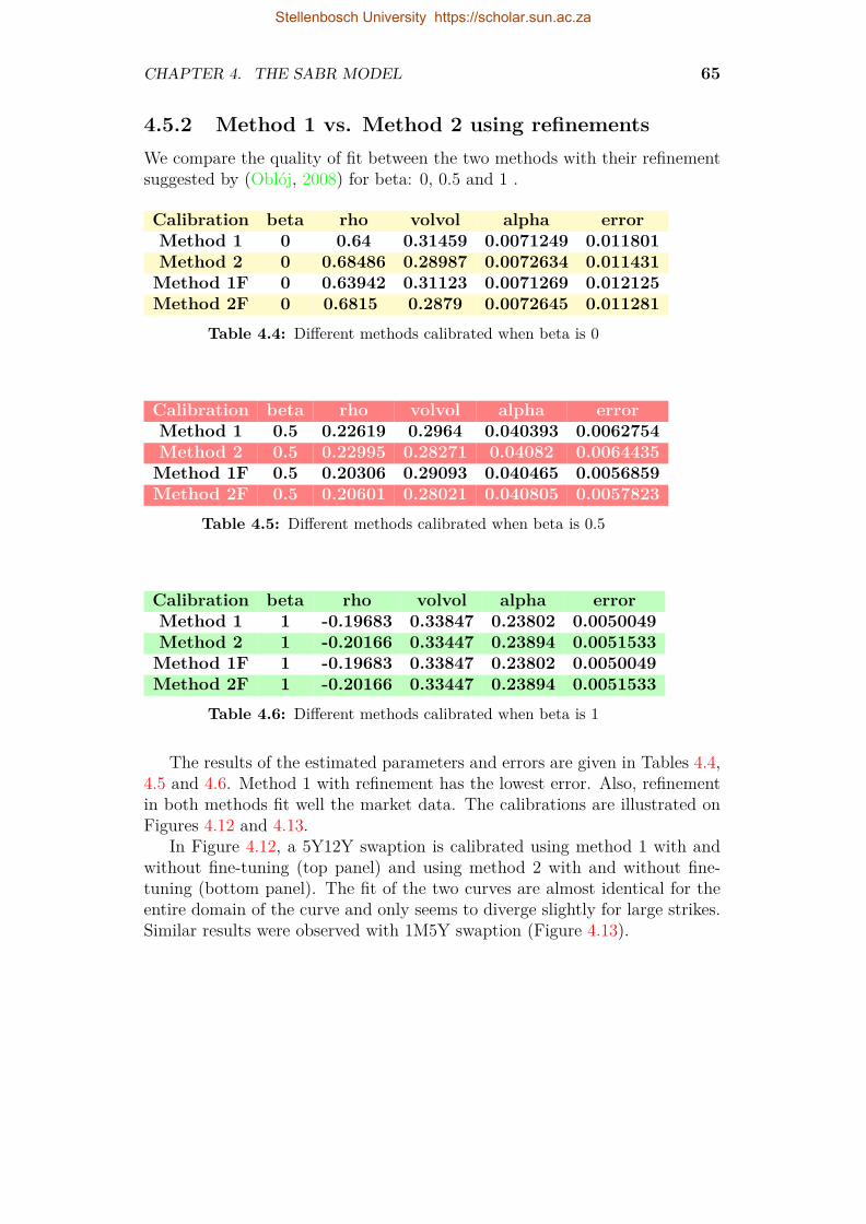
CHAPTER 4. THE SABR MODEL 65
4.5.2 Method 1 vs. Method 2 using refinementsWe compare the quality of fit between the two methods with their refinementsuggested by (Oblój, 2008) for beta: 0, 0.5 and 1 .
Calibration beta rho volvol alpha errorMethod 1 0 0.64 0.31459 0.0071249 0.011801Method 2 0 0.68486 0.28987 0.0072634 0.011431Method 1F 0 0.63942 0.31123 0.0071269 0.012125Method 2F 0 0.6815 0.2879 0.0072645 0.011281
Table 4.4: Different methods calibrated when beta is 0
Calibration beta rho volvol alpha errorMethod 1 0.5 0.22619 0.2964 0.040393 0.0062754Method 2 0.5 0.22995 0.28271 0.04082 0.0064435Method 1F 0.5 0.20306 0.29093 0.040465 0.0056859Method 2F 0.5 0.20601 0.28021 0.040805 0.0057823
Table 4.5: Different methods calibrated when beta is 0.5
Calibration beta rho volvol alpha errorMethod 1 1 -0.19683 0.33847 0.23802 0.0050049Method 2 1 -0.20166 0.33447 0.23894 0.0051533Method 1F 1 -0.19683 0.33847 0.23802 0.0050049Method 2F 1 -0.20166 0.33447 0.23894 0.0051533
Table 4.6: Different methods calibrated when beta is 1
The results of the estimated parameters and errors are given in Tables 4.4,4.5 and 4.6. Method 1 with refinement has the lowest error. Also, refinementin both methods fit well the market data. The calibrations are illustrated onFigures 4.12 and 4.13.
In Figure 4.12, a 5Y12Y swaption is calibrated using method 1 with andwithout fine-tuning (top panel) and using method 2 with and without fine-tuning (bottom panel). The fit of the two curves are almost identical for theentire domain of the curve and only seems to diverge slightly for large strikes.Similar results were observed with 1M5Y swaption (Figure 4.13).
Stellenbosch University https://scholar.sun.ac.za

CHAPTER 4. THE SABR MODEL 66
Figure 4.12: Top panel: 5Y12Y swaption calibration using Method 1, blue:SABR calibration using (Hagan et al., 2002) formulae, black: SABR calibrationusing (Oblój, 2008) (refinement). Bottom panel: 5Y12Y swaption calibration us-ing Method 2, blue: SABR calibration using (Hagan et al., 2002) formulae, black:SABR calibration using (Oblój, 2008) (refinement). Red: market volatilities, green:at the money.
Stellenbosch University https://scholar.sun.ac.za

CHAPTER 4. THE SABR MODEL 67
Figure 4.13: Top panel: 1M5Y swaption calibration using Method 1, blue:SABR calibration using (Hagan et al., 2002) formulae, black: SABR calibrationusing (Oblój, 2008) (refinement). Bottom panel: 1M5Y swaption calibration us-ing Method 2, blue: SABR calibration using (Hagan et al., 2002) formulae, black:SABR calibration using (Oblój, 2008) (refinement). Red: market volatilities, green:at the money.
Stellenbosch University https://scholar.sun.ac.za

CHAPTER 4. THE SABR MODEL 68
4.5.3 Calibration for long and short tenorsFor both methods and for a chosen beta, we have seen that the SABR modelhas a good fitness to a 1M5Y swaptions and 5Y12Y swaptions. Other com-binations of swaptions are possible, for this reason we look at the followingswaptions: 1M4Y, 20Y4Y, 1M20Y, 20Y20Y.
In Figures 4.14 and 4.15, the SABR model is calibrated for a 1M4Y anda 20Y4Y swaption (in this order) for β = 0.5 and β = 1. In Figure 4.16 theSABR model is calibrated for a 1M20Y and a 20Y20Y swaption for β = 0.5.The calibrated parameters: ρ, ν, α as well as sse can be found in Table 4.7.The 1M4Y and 20Y4Y swaptions for β = 0.5 (top panels of Figures 4.14 and4.15) do not have a good fitness. The fitness is even horrible with β = 0. Inthis case we did not report the figure, nevertheless, we can see how big is theerror in Table 4.7. However, we can see a “quite” good fitness when β = 1(bottom panels of Figures 4.14 and 4.15). In contrast, the 1M20Y and 20Y20Yswaptions for β = 0.5 do have a very good fitness (Figure 4.16). We underlinethat, the choice of beta in some scenarios is crucial as we have seen with the1M4Y and 20Y4Y swaptions. Another way to get a good fitness maybe to trywith refinements. This can be seen as a proof of the complexity and dynamicthe market.
The SABR model in (Hagan et al., 2002) was developed before the creditcrunch (interest rates were still somewhat high). But after the crisis, thedynamics of interest rates have changed, as we have seen in Chapter 3. Themarket has witnessed scenarios such as: negative interest rate and negativestrikes! The SABR model breaks down and we can no longer calibrate thecurve under methods presented so far, consequently we need methods thataccount for negative strikes.
Swaption alpha beta rho volvol error1M4Y 0.0080242 0 0.53584 0.51626 0.054251M5Y 0.008953 0 0.447103 0.651421 0.0247571M20Y 0.0091167 0 0.22047 0.73638 0.01217720Y4Y 0.0049645 0 1 0.26013 0.1354220Y20Y 0.0048115 0 0.39135 0.17722 0.00947051M4Y 0.053886 0.5 0.089563 0.54186 0.0426981M5Y 0.057738 0.5 0.08426 0.673686 0.0145631M20Y 0.05122 0.5 -0.034454 0.76423 0.005479120Y4Y 0.031644 0.5 1 0.061883 0.01552320Y20Y 0.026842 0.5 -0.1098 0.20861 0.00505511M4Y 0.36249 1 -0.27541 0.67734 0.0254631M5Y 0.373115 1 -0.24621 0.783108 0.0144821M20Y 0.28813 1 -0.26626 0.83733 0.008297520Y4Y 0.23422 1 -0.49579 0.12601 0.01139920Y20Y 0.16128 1 -0.42515 0.2771 0.0058998
Table 4.7: Some swaptions calibrated with Method 1 of (Hagan et al., 2002).
Stellenbosch University https://scholar.sun.ac.za

CHAPTER 4. THE SABR MODEL 69
Figure 4.14: Top panel: 1M4Y swaption calibration using Method 1 for β = 0.5.Bottom panel: 1M4Y swaption calibration using Method 1 for β = 1. Blue: SABRcalibration using (Hagan et al., 2002) formulae, red: market volatilities, green: atthe money.
Stellenbosch University https://scholar.sun.ac.za

CHAPTER 4. THE SABR MODEL 70
Figure 4.15: Top panel: 20Y4Y swaption calibration using Method 1 for β = 0.5.Bottom panel: 20Y4Y swaption calibration using Method 1 for β = 1. Blue: SABRcalibration using (Hagan et al., 2002) formulae, red: market volatilities, green: atthe money.
Stellenbosch University https://scholar.sun.ac.za

CHAPTER 4. THE SABR MODEL 71
Figure 4.16: Top panel: 1M20Y swaption calibration using Method 1 for β = 0.5.Bottom panel: 20Y20Y swaption calibration using Method 1 for β = 0.5. Blue:SABR calibration using (Hagan et al., 2002) formulae, red: market volatilities, green:at the money.
Stellenbosch University https://scholar.sun.ac.za

CHAPTER 4. THE SABR MODEL 72
4.6 Summary and conclusionIn this chapter, we have reviewed and calibrated the SABR model for differentswaptions. We have used two different methods (with and without refinement),we have found that the SABR model accurately capture the volatility smiles onthe markets. There is no considerable difference between both methods. Wehave found that refinements (produce smaller errors) may be good candidatefor a better fitness. We have also seen that, in some scenarios, the claim that“the choice of the parameter beta has no effect on the smile” is not true ingeneral.
This work can be extended to studying how to calculate swaptions, caps orfloors prices, and how they are affected by changing the parameters under theSABR model 3. Moreover, an extension of the SABR model that is consistentfor negative strikes is needed.
3this is the object of the next chapter ( Chapter 5)
Stellenbosch University https://scholar.sun.ac.za

Chapter 5
Interest rate curves and SABRcalibration applications
In this chapter, we consider problems that use interest rate curves and SABRCalibration. Particularly, we consider a method for transforming the marketobserved smile to non-standard tenors by applying the SABR model for arobust bootstrap of the whole smile. We use the results described in Chapters2, 3 and 4.
5.1 IntroductionAssuming that information on volatility smiles is provided by the market di-rectly through quotes of swaption smiles. Due to the fact that not everyswaption in the standard at-the-money matrix has also quotes for away-fromthe-money strikes and when quotes are often too few to allow for a robustbootstrap of the whole smile; the following question, therefore, arise naturallyin the current interest-rate volatility market:
• what is the value of implied volatility for strikes outside (and in particularlarger than) the quoted ones?
To answer such question rigorously, one should in principle resort to adynamical interest-rate model. Assuming, for instance, specific forward-ratedynamics, as in the Libor market models of (Piterbarg, 2003), (Errais et al.,2004) or (Henry-Labordere, 2006), one can employ suitable approximationsfor swaption prices calibrate the market swaption smiles. With the calibratedparameters, one can then price swaptions with any strike. However, evenneglecting the issue of accuracy of the approximations, this approach may betoo time-consuming and does not necessarily grant the precision required fora good estimate of the missing volatility values. In fact, model parameters aretypically too many for the calibration to be fast and, at the same time, toofew to recover (almost) exactly the quoted market data. One can thus prefer
73
Stellenbosch University https://scholar.sun.ac.za

CHAPTER 5. INTEREST RATE CURVES AND SABR CALIBRATIONAPPLICATIONS 74
to resort to a less elegant solution, which however answers the above questionin a rapid and consistent way.
In this chapter, we will then propose an empirical, yet consistent, procedurethat serves this purpose. To this end, we will use the functional form forimplied volatility derived by Hagan et al. (2002) which has been described inChapter 4. This work was partly done by Mercurio and Pallavicini (2006)in the single curve framework, in this chapter we extend the work in themulti-curve framework and this constitute one of our main contribution. Thisresult shows how to transform the market observed smile to non-standardtenors by applying the SABR model for a robust bootstrap of the whole smile.This shows as well the robustness of the SABR model to calibrate the marketvolatility smile coherently with the new market evidences as did Bianchettiand Carlicchi (2011).
5.2 Swaption smile and SABR functionalform
We consider, in the same chapter 2, the ATM strike defined in equation (2.3.5)as the forward swap rate defined in equation (2.5.6). Therefore, we can adaptthe result got in chapter 4 as follows.
Under the T -forward measure, the SABR model is described by the follow-ing system of stochastic differential equations:
dS(t, k, n) = α[S(t, k, n)
]βdW1, (5.2.1)
dα = ναdW2, α(0) = α (5.2.2)
E[dW1dW2] = ρdt (5.2.3)
where, S(0, k, n) is ATM strike, α is the volatility, and W1 and W2 are twocorrelated Wiener processes. The implied volatility σB
(S(0, k, n), K
)is ap-
proximately given by:
σB(S(0, k, n), K
)' U
(z
X(z)
)V (5.2.4)
where
U = α
[S(0, k, n)K](1−β)/2
[1 + (1−β)2
24 log2(S(0,k,n)
K
)+ (1−β)4
1920 log4(S(0,k,n)
K
)]−1
(5.2.5)
Stellenbosch University https://scholar.sun.ac.za

CHAPTER 5. INTEREST RATE CURVES AND SABR CALIBRATIONAPPLICATIONS 75
V =
1 +[
(1−β)2
24α2[
S(0,k,n)K]1−β + ρβνα
4[S(0,k,n)K
](1−β)/2 + 2−3ρ2
24 ν2]tex + . . .
. (5.2.6)
Here
z = να
[S(0, k, n)K
](1−β)/2log
(S(0,k,n)
K
)(5.2.7)
and X(z) is defined by
X(z) = log√
1−2ρz+z2+z−ρ1−ρ
. (5.2.8)
Where S(0, k, n) is given by
S(0, k, n) = P (0, Tk)− P (0, Tn)∑ni=k+1 δ(Ti−1, Ti)P (0, Ti)
. (5.2.9)
Formula (5.2.4) provides us with an (efficient) approximation for the SABRimplied volatility for each strike K. Its simplicity, combined with the intuitivemeaning of model parameters, has made it a popular choice for swaption smileanalysis, to the point of becoming a market standard for modelling impliedvolatility (this happened despite the fact that such approximation can lead toarbitrage opportunities for long maturities and large strike values).
We emphasis that, the procedure of calibration remains the same we didin Chapter 4. The only difference being in substituting the forward rate f inChapter 4 by S(0, k, n) in equation (5.2.9). However, S(0, k, n) in equation(5.2.9) requires the construction of the discount curve, and this was the objectof Chapter 2. We have to underline that changing f by S(0, k, n) in thecalibration process will slightly affect the values of the SABR parameters aswe will see in the example below.
In the multi-curve framework, as we have presented in Chapter 3, theprocedure is the same as above (formulae (5.2.1) to (5.2.8) remain valid).The only difference being in finding S(0, k, n). In the multi-curve framework,S(0, k, n) is given by
S(0, k, n) =∑ni=k δ(Ti−1, Ti)Pc(0, Ti)F (0;Ti−1, Ti)∑n
i=1 δ(Ti−1, Ti)Pc(0, Ti). (5.2.10)
S(0, k, n) in equation (5.2.10) requires the construction of the forward curveand discount curve, and this was treated in Chapter 3.
Example 5.1. This example shows to calibrate the multi-curve data for volatil-ity smiles. This is in the same way a methodology for transferring the shapeof the smile to non-standard tenors. To this end we have chosen the SABR
Stellenbosch University https://scholar.sun.ac.za

CHAPTER 5. INTEREST RATE CURVES AND SABR CALIBRATIONAPPLICATIONS 76
parameters β = 0.75, ρ = 0.47, ν = 0.76 and T = 3.5. The forward swap ratesare S(t, k, n) = 0.000792831267250977 (in the multi-curve) and S(t, k, n) =0.0252819292623 (in the single-curve). We take the volatility σ = 0.6743.Once we have the ATM volatility derived by the transformation method we cal-culate the parameter α to determine a SABR model with the new transformedvolatility. The corresponding SABR parameters are calculated using equation(3.3.7) and are given by α = 0.0912330160542767, α = 0.2167334588286166.As expected in Figure 4.6, the shape of the smile is preserved in terms of mon-eyness. After transforming the whole smile for non-standard tenors we areable to calculate swaptions, caps or floors prices, and how they are affectedby changing the parameters under the SABR model1 as we have announced inChapter 4.
5.3 Summary and conclusionIn this chapter, we have proposed an extension of a procedure for strippingconsistently implied volatilities in the multi-curve framework. We have high-lighted the procedure of the SABR calibration after the crisis. We claim that,after the crisis, the calibration procedure of the SABR model remain the sameas before the crisis. However the values of the parameters may vary (Example5.1 show the case in the value of the parameter α).
1formulae for this purpose are presented in the previous chapters
Stellenbosch University https://scholar.sun.ac.za

Chapter 6
Conclusion
In Chapter 2, we have introduced the methodologies for construction interestrate curves. We have reviewed the fundamental pricing formulas for plainvanilla interest rate derivatives in the classical framework with no collateral.Also, we have implemented the methodologies (Bootstrapping and Best Fit)for constructing discounting and forward yield curves.
In Chapter 3, we have given an overview of the changes that have takenplace in the financial markets since the credit crunch of 2007. No longer can weuse single-curve models when pricing and hedging plain vanilla single-currencyinterest rate derivatives. Instead, we use multiple distinct curves to ensuremarket coherent estimation of discount factors and of forward rates with differ-ent underlying rate tenors. We have reviewed the fundamental pricing formulasfor plain vanilla interest rate derivatives, extending the single-curve frameworkto the modern market situation with collateral.
In Chapter 4, we have reviewed and calibrated the SABRmodel for differentswaptions. We have used two different methods (with and without refinement),we have found that the SABR model accurately capture the volatility smileson the markets. There is no considerable difference between both methods.We have found that refinements may be a good candidate for a better fitness.We have also seen that, in some scenarios, the choice of the parameter betahas effect on the smile. In addition, from the same source of data, we haveseen that the value of the parameter beta that procedure a “good” fitness isnot the same for all the swaptions (this shows the complexity of the marketafter the credit crunch).
In Chapter 5, we have proposed an extension of a procedure for strippingconsistently implied volatilities in the multi-curve framework. Further workcan extend the procedure to strip CMS swap spreads. We have highlightedthe procedure of the SABR calibration after the crisis.
On the whole, we can see that the SABR functional form can calibrateconsistently implied volatilities in the multi-curve framework. Furthermore,it can well interpolate and extrapolate swap-rate volatility data and it is aneffective tool for pricing simple derivatives such as caps and floors, which are
77
Stellenbosch University https://scholar.sun.ac.za

CHAPTER 6. CONCLUSION 78
very sensitive to the swaption smile, without resorting to a fully-consistentinterest-rate model.
Finally, the work presented in this thesis can be extended in many direc-tions. We need a reconstruction of the interest rate modelling framework in apost-crisis financial world, with Libor rates incorporating credit and liquidityrisks. We need to include the cost of funding in constructing the OIS dis-counting yield curve and we need to include basis spreads in constructing ofmultiple forwarding yield curves.
Another extension will be to describe separately the discount and forwardyield curves using general short term interest rate models such as: Ho and Lee(1986), Hull and White (1993), Kalotay, Williams and Fabozzi (1993), Blackand Karasinski (1991), Black, Derman and Toy (1990), etc.
The short term interest rate models for the discount and forward interestrates need not to be the same in general. We can then approximate continuoustime models on discrete lattice, calculate interest rate trees (binomial or tri-nomial) for both discount and forward rates and calculate the cash flows treeusing both discount and forward rates. This approach (proposed by Oleksandret al. (2014)) can be used for pricing any interest rate derivative. In addition,this approach can be extended by considering affine jump diffusion interestrate models or lévy term structure models.
We need to compute the delta sensitivity of a portfolio consisting of instru-ments with a variety of different tenors, the convexity and other Greeks. Itis important to develop the model which can handle multiple dynamic curvesand its practical calibration scheme.
Stellenbosch University https://scholar.sun.ac.za

Appendices
79
Stellenbosch University https://scholar.sun.ac.za

Appendix A
Numéraire change
Let (Ω,F ,P,Ft) be a filtered probability space describing the market.
Definition A.1 (Numéraire ). A numéraire is a particular tradable asset ora tradable economic entity that can be used to express the relative prices of allother tradables in terms of its price. The relative price (relative to N) for anysecurity S, for a given numéraire asset N , is defined by:
S
N.
A numéraire must have strictly positive value, and must not have inter-mediate cash payments. There are many assets (or portfolios) that could bechosen as a numéraire. A numéraire is chosen for convenience only, and for noother reason. The choice of numéraire does not affect eventual prices in anyway.
Definition A.2 (Equivalent Martingale Measure (EMM)). A measure QN isan Equivalent Martingale Measure (EMM) relative to the numéraire N if
1. QN is equivalent to the probability measure P i.e. they have the same nullsets
P(X) = 0 if and only if QN(X) = 0 for any X ∈ F
2. QN is a martingale measure relative to N i.e. all relative prices aremartingales under QN
S(t)Nt
= EQN[S(T )NT
∣∣∣∣∣Ft]. (A.0.1)
We assume that the market is a well-functioning market, in other words,there is no arbitrage opportunities in the market1.
1Arbitrage opportunities represent the limitless creation of wealth through risk-freeprofit
80
Stellenbosch University https://scholar.sun.ac.za

APPENDIX A. NUMÉRAIRE CHANGE 81
Based on this assumption, we use the result “Market is free of arbitrageif and only if there exists an EMM (say QY )” established by (Harrison andKreps, 1979), (Harrison and Pliska, 1981) and (Harrison and Pliska, 1983) .
The natural question one may ask now is: what is this EMM QY ?
Proposition A.3. Since the choice of numéraire is irrelevant (we refer to(Ekstrand, 2011) for more details), if there exists an EMM QN relative tonuméraire N then for any other numéraireM there exists an EMM QM relativeto M .
From this proposition, we can deduce thatQY is equivalent to the EMMQB
(corresponding to the bank account from Definition 2.2) often called the risk-neutral measure. Hence if P (t, T ) (Definition 2.3) is taken as the numéraire(i.e. Nt = P (t, T )), then using formula (A.0.1), we have QN = QT 2 and
S(t) = P (t, T )EQT[S(T )
∣∣∣Ft]. (A.0.2)
Similarly, if Pc(t, T ) is the numéraire (i.e. Nt = Pc(t, T )), then we have
S(t) = Pc(t, T )EQTc[S(T )
∣∣∣Ft]. (A.0.3)
Formulae (A.0.2) and (A.0.3) are tools for pricing, we use Formula (A.0.2)in the market with no-collateralisation (before the crisis) and (A.0.3) in themarket with collateralisation (after the crisis, where the subscript c stands forunder CSA).
2discounting Tj-forward measure QTj , associated to the numéraire P (t, Tj)
Stellenbosch University https://scholar.sun.ac.za

Appendix B
Day Count Conventions
The different types of day count are: Actual/Actual, Actual/365, Actual/360and 30/360.
• Actual/Actual: (Actual/365, Actual/360) means that the accrued inter-est between the two given dates is calculated using the exact numberof calendar days between the two dates divided by the exact number ofcalendar days of the ongoing year (365, 360). For example, using theActual/Actual or Actual/365 day-count basis, there are 65 days from04/03/2013 to 06/07/2013. Using the Actual/365 day-count basis, theperiod from 03/07/2011 to 04/09/2013 converted in years is
299365 + 1 + 99
365 = 763365 = 2.090.
Using the Actual/360 day-count basis, the period from 03/07/2011 to04/09/2013 converted in years is
763360 = 2.1194.
• 30/360: means that the number of the calendar days between the twodates is computed assuming that each month count as 30. For instance,there are 75 days (2× 30 + 15) from 02/04/2013 to 04/19/2013 and 277days (9 × 30 + 7) from 03/11/2013 to 12/18/2013. Using the 30/360day-count basis, the period from 03/07/2011 to 04/09/2013 converted inyears is
25× 30 + 2360 = 2.0888.
82
Stellenbosch University https://scholar.sun.ac.za

Appendix C
Interpolation and LMA
This appendix presents some interpolation methods and the Levenberg-Marquardtalgorithm.
C.1 Linear interpolationLet P := a = x0 < x1 < x2 < ... < xn = b be a partition of the interval[a, b].
Definition C.1. A Linear Interpolation (function) LP on L is a real functionLP : [a, b]→ R with the property: LP coincides on every subinterval [xi, xi+1],i = 0, 1, . . . , n− 1, with a polynomial of degree one.
Let Y := y0, y1, . . . yn, LP (Y ; .) an linear Interpolation function LP withLP (Y ;xi) = yi for i = 0, 1, . . . , n and hi+1 = xi+1 − xi, for i = 0, 1, . . . , n− 1.We prove that
LP (Y ;x) = yixi+1 − xhi+1
+ yi+1x− xihi+1
for x ∈ [xi, xi+1].
Linear interpolation is often used to approximate a value of some function Gusing two known values of that function at other points (for instance x = uand x = v). The error of this approximation is defined as
RT = G(x)− LP (Y ;x)
By virtue of It can be proven using Rolle’s theorem1 we can prove that:
LP (Y ;x) = G(u) + G(v)−G(u)v − u
(x− u).1 Rolle’s theorem If a real-valued function f is continuous on a closed interval [a, b],
differentiable on the open interval (a, b), and f(a) = f(b), then there exists a c in the openinterval (a, b) such that f ′(c) = 0.
83
Stellenbosch University https://scholar.sun.ac.za

APPENDIX C. INTERPOLATION AND LMA 84
with the error term bounded by:
|RT | ≤(u− v)2
8 maxu≤x≤v
|G′′(x)|.
Linear interpolation can be applied on rates, logarithm of rates, discount fac-tors, logarithm of discount factor and on forward rates.
C.2 Cubic splinesLet P := a = x0 < x1 < x2 < ... < xn = b be a partition of the interval[a, b].
Definition C.2. A cubic spline (function) SP on P is a real function SP :[a, b]→ R with the properties:
(1) SP ∈ C2[a, b], that is, SP is twice continuously differentiable on [a, b].
(2) SP coincides on every subinterval [xi, xi+1], i = 0, 1, . . . , n − 1, with apolynomial of degree three.
Let Y := y0, y1, . . . yn, SP (Y ; .) an interpolating spline function SP withSP (Y ;xi) = yi for i = 0, 1, . . . , n and hi+1 = xi+1 − xi, for i = 0, 1, . . . , n− 1.
Such SP is not unique, the following three conditions by itself ensuresuniqueness of SP (it has been proved in (Bulirsch and Stoer, 2002))
(i) S ′′P (Y ; a) = S ′′P (Y ; b) = 0,
(ii) SmP (Y ; a) = SmP (Y ; b) = 0, for m = 0, 1, 2: SP (Y ; .) is periodic,
(iii) S ′P (Y ; a) = γ0, S ′P (Y ; b) = γn, for given γ0, γn.
Let the values of the second derivatives at xi ∈ P , be defined by
Mi := S ′′P (Y ;xi), i = 0, 1, · · · , n. (C.2.1)
Property (2) in definition C.2, implies that S ′′P (Y ; .) is a linear function in each[xi, xi+1], i = 0, 1, . . . , n− 1. Therefore, S ′′P (Y ; .) can be written as
S ′′P (Y ;x) = Mixi+1 − xhi+1
+Mi+1x− xihi+1
for x ∈ [xi, xi+1].
By successive integration, for x ∈ [xi, xi+1] and i = 0, 1, . . . , n− 1, we have
S ′P (Y ;x) = −Mi(xi+1 − x)2
2hi+1+Mi+1
(x− xi)2
2hi+1+ Ai,
SP (Y ;x) = Mi(xi+1 − x)3
6hi+1+Mi+1
(x− xi)3
6hi+1+ Ai(x− xi) +Bi.
(C.2.2)
Stellenbosch University https://scholar.sun.ac.za

APPENDIX C. INTERPOLATION AND LMA 85
Using the fact SP (Y ;xi) = yi and SP (Y ;xi+1) = yi+1, we obtain
Bi = yi −Mih2i+16 ,
Ai = yi+1 − yihi+1
− hi+1
6 (Mi+1 −Mi).(C.2.3)
Substituting (C.2.3) in (C.2.2) yields
S ′P (Y ;x) = −Mi(xi+1 − x)2
2hi+1+Mi+1
(x− xi)2
2hi+1+ yi+1 − yi
hi+1− hi+1
6 (Mi+1 −Mi).
For j = 1, 2, · · · , n− 1, we have therefore
S ′P (Y ;x−) = yi − yi−1
hi+ hi
3 Mi + hi6 Mi−1,
S ′P (Y ;x+) = yi+1 − yihi+1
− hi+1
3 Mi −hi+1
6 Mi+1.
The continuity of S ′P (Y ; .) at x = xi implies that S ′P (Y ;x−) = S ′P (Y ;x+),hence for j = 1, 2, · · · , n− 1 we have
hi6 Mi−1 + hi + hi+1
3 Mi + hi+1
6 Mi+1 = yi+1 − yihi+1
− yi − yi−1
hi. (C.2.4)
Using the conditions (i), (ii) and (iii) above, we have
• Case(i):S ′′P (Y ; a) = M0 = Mn = S ′′P (Y ; b).
• Case(ii):
S ′′P (Y ; a) = S ′′P (Y ; b) =⇒M0 = Mn;
S ′P (Y ; a) = S ′P (Y ; b) =⇒ hn6 Mn−1 + hn + h1
3 Mn + h1
6 M1
= y1 − ynh1
− yn − yn−1
hn.
The latter condition is identical to (C.2.4) for i = n if we put
hn+1 := h1, Mn+1 := M1, yn+1 := y1.
• Case(iii):
S ′P (Y ; a) = y′0 =⇒ h1
3 M0 + h1
6 M1 = y1 − y0
h1− y′0.
S ′P (Y ; b) = y′n =⇒ hn6 Mn−1 + hn
3 Mn = y′n −yn − yn−1
hn
Stellenbosch University https://scholar.sun.ac.za

APPENDIX C. INTERPOLATION AND LMA 86
The last two equations and those in (C.2.4) can be written as
µiMi−1 + 2Mi + λjMi+1 = di, j = 1, 2, . . . n− 1,
where
λi : = hi+1
hi + hi+1, µi := 1− λi = hi
hi + hi+1
di : = 6hi + hi+1
yi+1 − yihi+1
− yi − yi−1
hi
In case (i), we define in addition
λ0 := 0, d0 := 0, µn := 0, dn := 0,
in case (iii)
λ0 := 1, d0 := 6h1
y1 − y0
h1− y′0
µn := 1, dn := 6
hn
y′n − yn − yn−1
hn
.finally in case (ii), we define
λn : = h1
hn + h1, µn := 1− λn = hn
hn + h1,
di : = 6hn + h1
y1 − ynh1
− yn − yn−1
hn
.
C.3 Levenberg-Marquardt algorithmThe Levenberg-Marquardt algorithm is an iterative procedure used to solvenon-linear least squares problems (especially in least squares curve fitting).The Levenberg-Marquardt curve-fitting method is a combination of two min-imization methods: the Gauss-Newton algorithm (GNA) and the gradientdescent method.
The problemGiven a set of n empirical datum pairs of independent and dependent variables,(xi, yi), optimize the parameters β of the model curve f(x, β) (where f is non-linear in β) so that the sum of the squares of the deviations
S(β) =m∑i=1
[yi − f(xi, β)]2 (C.3.1)
becomes minimal.
Stellenbosch University https://scholar.sun.ac.za
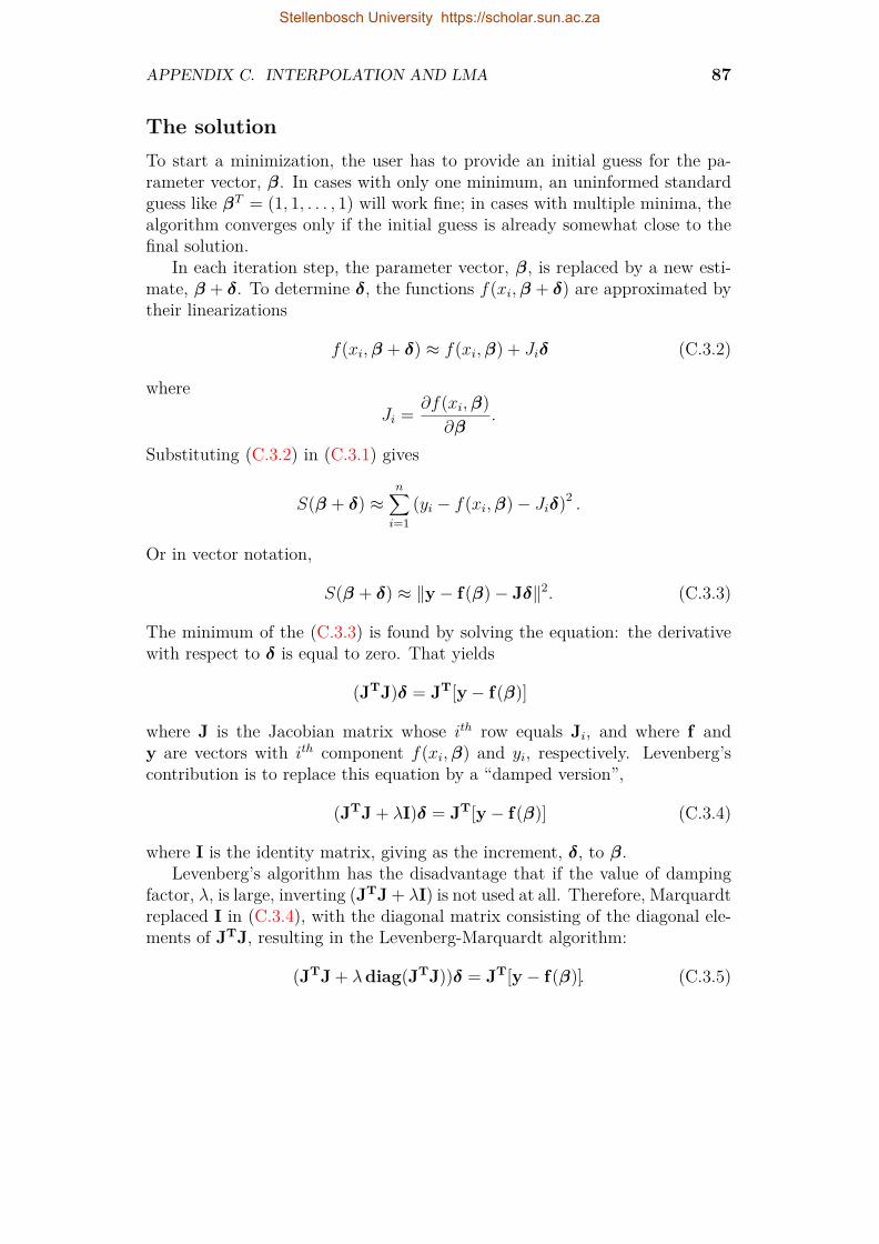
APPENDIX C. INTERPOLATION AND LMA 87
The solutionTo start a minimization, the user has to provide an initial guess for the pa-rameter vector, β. In cases with only one minimum, an uninformed standardguess like βT = (1, 1, . . . , 1) will work fine; in cases with multiple minima, thealgorithm converges only if the initial guess is already somewhat close to thefinal solution.
In each iteration step, the parameter vector, β, is replaced by a new esti-mate, β + δ. To determine δ, the functions f(xi,β + δ) are approximated bytheir linearizations
f(xi,β + δ) ≈ f(xi,β) + Jiδ (C.3.2)
whereJi = ∂f(xi,β)
∂β.
Substituting (C.3.2) in (C.3.1) gives
S(β + δ) ≈n∑i=1
(yi − f(xi,β)− Jiδ)2 .
Or in vector notation,
S(β + δ) ≈ ‖y− f(β)− Jδ‖2. (C.3.3)
The minimum of the (C.3.3) is found by solving the equation: the derivativewith respect to δ is equal to zero. That yields
(JTJ)δ = JT[y− f(β)]
where J is the Jacobian matrix whose ith row equals Ji, and where f andy are vectors with ith component f(xi,β) and yi, respectively. Levenberg’scontribution is to replace this equation by a “damped version”,
(JTJ + λI)δ = JT[y− f(β)] (C.3.4)
where I is the identity matrix, giving as the increment, δ, to β.Levenberg’s algorithm has the disadvantage that if the value of damping
factor, λ, is large, inverting (JTJ + λI) is not used at all. Therefore, Marquardtreplaced I in (C.3.4), with the diagonal matrix consisting of the diagonal ele-ments of JTJ, resulting in the Levenberg-Marquardt algorithm:
(JTJ + λdiag(JTJ))δ = JT[y− f(β)]. (C.3.5)
Stellenbosch University https://scholar.sun.ac.za

Appendix D
Data
D.1 Interest rate dataThe market data presented here can be found in (Ametrano and Bianchetti,2013).
Quote Settlement Business Day End of MonthInstrument (ask, %) Underlying Start Date Maturity Date rule Convention Convention
Depo ON 0.040 Euribor1D Tue 11 Dec 2012 Wed 12 Dec 2012 Today Following False... ... ... ... ... ... ... ...
Depo 12M 0.540 Euribor12M Thu 13 Dec 2012 Fri 13 Dec 2013 Spot Mod.Following True
Table D.1: EUR Deposit strip. Source: Reuters page KLIEM, 11 Dec. 2012.
Quote Quote QuoteInstrument (bid, %) (ask, %) (mid, %) Underlying Start Date Maturity
FRA Tod3M 0.156 0.206 0.181 Euribor3M Thu 13 Dec 2012 Wed 13 Mar 2013FRA Tom3M 0.154 0.204 0.179 Euribor3M Fri 14 Dec 2012 Thu 14 Mar 2013FRA 1x4 0.140 0.190 0.165 Euribor3M Mon 14 Jan 2013 Mon 15 Apr 2013... ... ... ... ... ... ...FRA Tod6M 0.291 0.341 0.316 Euribor6M Thu 13 Dec 2012 Thu 13 Jun 2013FRA Tom6M 0.287 0.337 0.312 Euribor6M Fri 14 Dec 2012 Fri 14 Jun 2013FRA 1x7 0.268 0.318 0.293 Euribor6M Mon 14 Jan 2013 Mon 15 Jul 2013... ... ... ... ... ... ...FRA 12x24 0.482 0.532 0.507 Euribor12M Fri 13 Dec 2013 Mon 15 Dec 2014FRA IMMF3 0.264 0.314 99.7110 Euribor6M Wed 16 Jan 2013 Tue 16 Jul 2013FRA IMMG3 0.244 0.294 99.7310 Euribor6M Wed 20 Feb 2013 Tue 20 Aug 2013FRA IMMH3 0.234 0.284 99.7410 Euribor6M Wed 20 Mar 2013 Fri 20 Sep 2013FRA IMMJ3 0.230 0.280 99.7450 Euribor6M Wed 17 Apr 2013 Thu 17 Oct 2013
Table D.2: EUR FRA strips on Euribor 3M, Euribor 6M, and Euribor 12M.
88
Stellenbosch University https://scholar.sun.ac.za

APPENDIX D. DATA 89
HW parameter Value
Mean reversion 3%
Volatility 0.3526%
Table D.3: Hull-White parameters values for Futures 3M convexity adjustment asof 11 Dec. 2012.
Quote Quote QuoteInstrument (bid, %) (ask, %) (mid, %) Convexity Underlying Underlying Start Underlying End
adjustment Date Date
FUT 3MZ2 99.8200 99.8250 99.8225 0.0000% Euribor3M Wed 19 Dec 2012 Tue 19 Mar 2013... ... ... ... ...% ... ... ...FUT 3MU7 98.4000 98.4250 98.4125 0.0136% Euribor3M Wed 20 Sep 2017 Wed 20 Dec 2017
Table D.4: EUR Futures on Euribor 3M, "H", "M", "U" and "Z" standing forMarch, June, September and December expiries, respectively and two serial Futures(denoted as F3, G3 for Jan. and Feb 2013 expiries) are displayed. Source: Reuterspage 0# FEI, as of 11 Dec. 2012. Column 5 reports the corresponding convexityadjustments.
Quote Quote QuoteInstrument (bid, %) (ask, %) (mid, %) Underlying Start Date Maturity
AB6E1Y 0.266 0.306 0.286 Euribor6M Thu 13 Dec 2012 Fri 13 Dec 2013... ... ... ... ... ... ...AB6E60Y 2.443 2.483 2.463 Euribor6M Thu 13 Dec 2012 Tue 18 Dec 2072
Table D.5: EUR IRS on Euribor 6M. The codes “AB6En” in col.1 label IRSreceiving annually a fixed rate and paying semi-annually a floating rate on Euribor6M with maturity in n months/years.
Quote Quote QuoteInstrument (bid, %) (ask, %) (mid, %) Underlying Start Date Maturity
AB3E1Y 0.116 0.166 0.141 Euribor3M Thu 13 Dec 2012 Fri 13 Dec 2013... ... ... ... ... ... ...AB3E50Y 2.342 2.392 2.367 Euribor3M Thu 13 Dec 2012 Wed 13 Dec 2062AB3EZ2 0.113 0.163 0.138 Euribor3M Wed 19 Dec 2012 Thu 19 Dec 2013... ... ... ... ... ... ...AB3EZ4 0.258 0.308 0.283 Euribor3M Wed 17 Jun 2014 Mon 18 Jun 2017
Table D.6: EUR IRS on Euribor 3M, receiving annually a fixed rate and payingquarterly a floating rate on Euribor 3M. At the bottom IMM starting IRS arereported, denoted with their corresponding IMM code.
Stellenbosch University https://scholar.sun.ac.za

APPENDIX D. DATA 90
Quote Quote QuoteInstrument (bid, %) (ask, %) (mid, %) Underlying Start Date Maturity
AB1E2M 0.081 0.131 0.106 Euribor1M Thu 13 Dec 2012 Wed 13 Feb 2013... ... ... ... ... ... ...AB1E12M 0.038 0.088 0.063 Euribor1M Thu 13 Dec 2012 Fri 13 Dec 2013
Table D.7: EUR IRS on Euribor 1M, receiving annually a fixed rate and payingmonthly a floating rate on Euribor 1M.
Quote Quote QuoteInstrument (bid, %) (ask, %) (mid, %) Underlying Start Date Maturity
EON1W 0.020 0.120 0.070 Eonia Thu 13 Dec 2012 Thu 20 Dec 2012... ... ... ... ... ... ...EON30Y 2.003 2.073 2.038 Eonia Thu 13 Dec 2012 Mon 15 Dec 2042EONCBFEB13 0.021 0.071 0.046 Eonia Wed 16 Jan 2013 Wed 13 Feb 2013EONCBMAR13 -0.009 0.041 0.016 Eonia Wed 13 Feb 2013 Wed 13 Mar 2013EONCBAPR13 -0.032 0.018 -0.007 Eonia Wed 13 Mar 2013 Wed 10 Apr 2013EONCBMAY13 -0.038 0.012 -0.013 Eonia Wed 10 Apr 2013 Wed 08 May 2013EONCBJUN13 -0.039 0.011 -0.014 Eonia Wed 08 May 2013 Wed 12 Jun 2013EONCBJUL13 -0.041 0.009 -0.016 Eonia Wed 12 Jun 2013 Wed 10 Jul 2013
Table D.8: EUR OIS, receiving an annual fixed rate and paying an annual floatingrate on Eonia. At the bottom forward starting OIS at known ECB dates. NegativesOIS rates are enlightened in blue color.
Instrument Quote(bps) Underlying 1st leg Underlying 2nd leg Start Date Maturity
1E6E1Y 22.20 Euribor1M Euribor6M Thu 13 Dec 2012 Fri 13 Dec 2013... ... ... ... ... ...1E6E30Y 16.30 Euribor1M Euribor6M Thu 13 Dec 2012 Mon 15 Dec 20423E6E1Y 14.50 Euribor3M Euribor6M Thu 13 Dec 2012 Fri 13 Dec 2013... ... ... ... ... ...3E6E50Y 5.40 Euribor3M Euribor6M Thu 13 Dec 2012 Wed 13 Dec 20626E12E1Y 26.20 Euribor6M Euribor12M Thu 13 Dec 2012 Fri 13 Dec 2013... ... ... ... ... ...6E12E30Y 6.60 Euribor6M Euribor12M Thu 13 Dec 2012 Mon 15 Dec 2042
Table D.9: EUR IRBS. The codes “xEyEnY" in col. 1 label basis swaps receivingEuribor xM and paying Euribor yM plus basis spread with n maturity years.
D.2 Swedish market (swaption) data1M 3M 6M 1Y 2Y 3Y 4Y 5Y 7Y 10Y 20Y
1Y 33.4 30.1 31.5 31.1 34.3 33.9 29.8 27.8 24.5 22.4 19.72Y 32.8 31.1 33.3 33.3 34 31.5 28.4 26.3 24.8 21.5 20.93Y 34 32.5 34.8 34.8 32 29.9 27.4 25.4 24.4 21.1 21.54Y 36.3 35 34.9 33.9 30.6 28.7 26.6 24.9 23.8 20.9 22.15Y 37.4 36.3 35.5 33.1 29.7 27.6 25.9 24.4 23.2 20.8 22.27Y 32.5 31.3 30.9 29.7 27.8 26.7 25.5 24.4 22.9 20.8 21.210Y 31.1 29.3 28.2 26.8 26.1 25.7 25.1 24.4 22.9 21.1 19.912Y 31.1 29.3 28.2 26.8 26.1 25.7 25.1 24.4 22.9 21.1 19.915Y 29.3 28 27.3 26.1 25.1 24.8 24.1 23 22.3 20.3 17.220Y 28.9 27.9 27.4 26.4 25 24.6 23.8 22.8 21.9 19.8 16.1
Stellenbosch University https://scholar.sun.ac.za

APPENDIX D. DATA 91
1YStrike Spread 1M 3M 6M 1Y 2Y 3Y 4Y 5Y 7Y 10Y 20Y
-0.568949 -2 59.9 59.9 45.4 26.3 24.8 17 13.98769 11 9.1 8.4 6.8-0.318949 -1.75 51.25 51.25 38.9 22.6 20.175 13.975 11.51495 9.075 7.5 6.925 5.625-0.068949 -1.5 42.6 42.6 32.4 18.9 15.55 10.95 9.042202 7.15 5.9 5.45 4.450.181051 -1.25 33.95 33.95 25.9 15.2 10.925 7.925 6.56946 5.225 4.3 3.975 3.2750.431051 -1 25.3 25.3 19.4 11.5 6.3 4.9 4.096717 3.3 2.7 2.5 2.10.681051 -0.75 16.65 16.65 12.9 7.8 4.35 3.4 2.847743 2.3 1.85 1.7 1.450.931051 -0.5 8 8 6.4 4.1 2.4 1.9 1.598769 1.3 1 0.9 0.81.181051 -0.25 3.1 3.1 2.6 1.7 1.1 0.9 0.749384 0.6 0.4 0.4 0.41.431051 0 0 0 0 0 0 0 0 0 0 0 01.681051 0.25 -1.4 -1.4 -1.4 -1.1 -0.7 -0.6 -0.49959 -0.4 -0.4 -0.3 -0.31.931051 0.5 -1.6 -1.6 -1.9 -1.8 -1.3 -1.2 -0.948974 -0.7 -0.6 -0.5 -0.62.181051 0.75 -1.05 -1.05 -1.8 -2.1 -1.7 -1.5 -1.198769 -0.9 -0.7 -0.55 -0.752.431051 1 -0.5 -0.5 -1.7 -2.4 -2.1 -1.8 -1.448564 -1.1 -0.8 -0.6 -0.92.681051 1.25 0.35 0.35 -1.15 -2.25 -2.2 -1.925 -1.523358 -1.125 -0.775 -0.55 -0.9752.931051 1.5 1.2 1.2 -0.6 -2.1 -2.3 -2.05 -1.598153 -1.15 -0.75 -0.5 -1.053.181051 1.75 2.05 2.05 -0.05 -1.95 -2.4 -2.175 -1.672948 -1.175 -0.725 -0.45 -1.1253.431051 2 2.9 2.9 0.5 -1.8 -2.5 -2.3 -1.747743 -1.2 -0.7 -0.4 -1.2
2YStrike Spread 1M 3M 6M 1Y 2Y 3Y 4Y 5Y 7Y 10Y 20Y
-0.280702 -2 40.5 40.5 31.6 40.8 19.5 13.9 11.84159 9.8 8.5 7.3 6.6-0.030702 -1.75 34.7 34.7 27.1 32.75 15.925 11.425 9.743126 8.075 6.975 5.95 5.4250.219298 -1.5 28.9 28.9 22.6 24.7 12.35 8.95 7.644665 6.35 5.45 4.6 4.250.469298 -1.25 23.1 23.1 18.1 16.65 8.775 6.475 5.546204 4.625 3.925 3.25 3.0750.719298 -1 17.3 17.3 13.6 8.6 5.2 4 3.447743 2.9 2.4 1.9 1.90.969298 -0.75 11.5 11.5 9.1 5.85 3.55 2.75 2.373461 2 1.65 1.3 1.351.219298 -0.5 5.7 5.7 4.6 3.1 1.9 1.5 1.299179 1.1 0.9 0.7 0.81.469298 -0.25 2.2 2.2 1.9 1.3 0.8 0.6 0.549795 0.5 0.4 0.3 0.31.719298 0 0 0 0 0 0 0 0 0 0 0 01.969298 0.25 -1.1 -1.1 -1.1 -0.9 -0.7 -0.5 -0.39959 -0.3 -0.2 -0.1 -0.32.219298 0.5 -1.3 -1.3 -1.6 -1.5 -1.1 -0.9 -0.699179 -0.5 -0.4 -0.2 -0.52.469298 0.75 -0.85 -0.85 -1.55 -1.75 -1.4 -1.15 -0.873871 -0.6 -0.45 -0.15 -0.652.719298 1 -0.4 -0.4 -1.5 -2 -1.7 -1.4 -1.048564 -0.7 -0.5 -0.1 -0.82.969298 1.25 0.35 0.35 -1.05 -1.925 -1.775 -1.425 -1.03591 -0.65 -0.425 0.025 -0.853.219298 1.5 1.1 1.1 -0.6 -1.85 -1.85 -1.45 -1.023256 -0.6 -0.35 0.15 -0.93.469298 1.75 1.85 1.85 -0.15 -1.775 -1.925 -1.475 -1.010602 -0.55 -0.275 0.275 -0.953.719298 2 2.6 2.6 0.3 -1.7 -2 -1.5 -0.997948 -0.5 -0.2 0.4 -1
3YStrike Spread 1M 3M 6M 1Y 2Y 3Y 4Y 5Y 7Y 10Y 20Y
-0.005595 -2 38.79689 38.79689 30.1 32.86667 16.80246 12.50128 10.90847 9.333333 8.233577 7.200091 7.0341240.244405 -1.75 32.6713 32.6713 25.35833 26.40833 13.70203 10.25107 8.951591 7.666667 6.74188 5.858417 5.7839870.494405 -1.5 26.54571 26.54571 20.61667 19.95 10.6016 8.000867 6.994712 6 5.250182 4.516743 4.533850.744405 -1.25 20.42012 20.42012 15.875 13.49167 7.501163 5.750661 5.037834 4.333333 3.758485 3.175068 3.2837140.994405 -1 14.29453 14.29453 11.13333 7.033333 4.40073 3.500456 3.080955 2.666667 2.266788 1.833394 2.0335771.244405 -0.75 9.479653 9.479653 7.433333 4.766667 2.98385 2.383668 2.106719 1.833333 1.53344 1.233394 1.4334851.494405 -0.5 4.664781 4.664781 3.733333 2.5 1.566971 1.26688 1.132483 1 0.800091 0.633394 0.8333941.744405 -0.25 1.79927 1.79927 1.5 1.033333 0.666788 0.500091 0.466378 0.433333 0.333394 0.266697 0.3333941.994405 0 0 0 0 0 0 0 0 0 0 0 02.244405 0.25 -0.866241 -0.866241 -0.866667 -0.7 -0.566788 -0.400091 -0.332938 -0.266667 -0.2 -0.133303 -0.32.494405 0.5 -1.032847 -1.032847 -1.2 -1.133333 -0.86688 -0.700182 -0.549111 -0.4 -0.366697 -0.2 -0.5333942.744405 0.75 -0.616241 -0.616241 -1.05 -1.283333 -1.083622 -0.883577 -0.673781 -0.466667 -0.383394 -0.15 -0.7000912.994405 1 -0.199635 -0.199635 -0.9 -1.433333 -1.300365 -1.066971 -0.79845 -0.533333 -0.400091 -0.1 -0.8667883.244405 1.25 0.508622 0.508622 -0.483333 -1.316667 -1.317085 -1.050342 -0.689976 -0.466667 -0.316766 0.025 -0.9251373.494405 1.5 1.21688 1.21688 -0.066667 -1.2 -1.333805 -1.033714 -0.681548 -0.4 -0.23344 0.15 -0.9834853.744405 1.75 1.925137 1.925137 0.35 -1.083333 -1.350525 -1.017085 -0.67312 -0.333333 -0.150114 0.275 -1.0418343.994405 2 2.633394 2.633394 0.766667 -0.966667 -1.367245 -1.000456 -0.664692 -0.266667 -0.066788 0.4 -1.100182
4YStrike Spread 1M 3M 6M 1Y 2Y 3Y 4Y 5Y 7Y 10Y 20Y
0.213859 -2 37.09845 37.09845 28.6 24.93333 14.10493 11.09872 9.977901 8.866667 7.966423 7.100182 7.4670620.463859 -1.75 30.64815 30.64815 23.61667 20.06667 11.47906 9.073928 8.162218 7.258333 6.50812 5.766834 6.1419940.713859 -1.5 24.19786 24.19786 18.63333 15.2 8.853193 7.049133 6.346535 5.65 5.049818 4.433485 4.8169250.963859 -1.25 17.74756 17.74756 13.65 10.33333 6.227327 5.024339 4.530853 4.0416667 3.591515 3.100137 3.4918571.213859 -1 11.29726 11.29726 8.666667 5.466667 3.60146 2.999544 2.71517 2.433333 2.133212 1.766788 2.1667881.463859 -0.75 7.464827 7.464827 5.766667 3.683333 2.41771 2.016332 1.840706 1.666667 1.41656 1.166788 1.5167431.713859 -0.5 3.632391 3.632391 2.866667 1.9 1.233942 1.03312 0.966241 0.9 0.699909 0.566788 0.8666971.963859 -0.25 1.399635 1.399635 1.1 0.766667 0.533577 0.399909 0.383189 0.366667 0.266606 0.233394 0.3666972.213859 0 0 0 0 0 0 0 0 0 0 0 02.463859 0.25 -0.63312 -0.63312 -0.633333 -0.5 -0.433577 -0.299909 -0.266469 -0.233333 -0.2 -0.166606 -0.32.713859 0.5 -0.766423 -0.766423 -0.8 -0.766667 -0.633759 -0.499818 -0.399453 -0.3 -0.333303 -0.2 -0.5666972.963859 0.75 -0.38312 -0.38312 -0.55 -0.816667 -0.767245 -0.616423 -0.474236 -0.333333 -0.316606 -0.15 -0.7500463.213859 1 0.000182 0.000182 -0.3 -0.866667 -0.90073 -0.733029 -0.54902 -0.366667 -0.299909 -0.1 -0.9333943.463859 1.25 0.666811 0.666811 0.083333 -0.708333 -0.85917 -0.674658 -0.344988 -0.283333 -0.208234 0.025 -1.0000683.713859 1.5 1.33344 1.33344 0.466667 -0.55 -0.817609 -0.616286 -0.340774 -0.2 -0.1165 0.15 -1.0667433.963859 1.75 2.000068 2.000068 0.85 -0.391667 -0.776049 -0.557915 -0.33656 -0.116667 -0.024886 0.275 -1.1334174.213859 2 2.666697 2.666697 1.233333 -0.233333 -0.734489 -0.499544 -0.332346 -0.033333 0.066788 0.4 -1.200091
5YStrike Spread 1M 3M 6M 1Y 2Y 3Y 4Y 5Y 7Y 10Y 20Y
0.399829 -2 35.4 35.4 27.1 17 11.4 9.7 9.047332 8.4 7.7 7 7.90.649829 -1.75 28.625 28.625 21.875 13.725 9.25 7.9 7.372845 6.85 6.275 5.675 6.50.899829 -1.5 21.85 21.85 16.65 10.45 7.1 6.1 5.698358 5.3 4.85 4.35 5.11.149829 -1.25 15.075 15.075 11.425 7.175 4.95 4.3 4.023871 3.75 3.425 3.025 3.71.399829 -1 8.3 8.3 6.2 3.9 2.8 2.5 2.349384 2.2 2 1.7 2.31.649829 -0.75 5.45 5.45 4.1 2.6 1.85 1.65 1.574692 1.5 1.3 1.1 1.61.899829 -0.5 2.6 2.6 2 1.3 0.9 0.8 0.8 0.8 0.6 0.5 0.92.149829 -0.25 1 1 0.7 0.5 0.4 0.3 0.3 0.3 0.2 0.2 0.42.399829 0 0 0 0 0 0 0 0 0 0 0 02.649829 0.25 -0.4 -0.4 -0.4 -0.3 -0.3 -0.2 -0.2 -0.2 -0.2 -0.2 -0.32.899829 0.5 -0.5 -0.5 -0.4 -0.4 -0.4 -0.3 -0.249795 -0.2 -0.3 -0.2 -0.63.149829 0.75 -0.15 -0.15 -0.05 -0.35 -0.45 -0.35 -0.274692 -0.2 -0.25 -0.15 -0.83.3998291 1 0.2 0.2 0.3 -0.3 -0.5 -0.4 -0.29959 -0.2 -0.2 -0.1 -13.649829 1.25 0.825 0.825 0.65 -0.1 -0.4 -0.3 0 -0.1 -0.1 0.025 -1.0753.899829 1.5 1.45 1.45 1 0.1 -0.3 -0.2 0 0 0 0.15 -1.154.149829 1.75 2.075 2.075 1.35 0.3 -0.2 -0.1 0 0.1 0.1 0.275 -1.2254.399829 2 2.7 2.7 1.7 0.5 -0.1 0 0 0.2 0.2 0.4 -1.3
Stellenbosch University https://scholar.sun.ac.za

APPENDIX D. DATA 92
7YStrike Spread 1M 3M 6M 1Y 2Y 3Y 4Y 5Y 7Y 10Y 20Y
0.673166 -2 31.03642 31.03642 24.13919 15.39956 11.12015 10.21972 10.07022 9.920416 9.259146 8.559146 8.6205910.923166 -1.75 25.24222 25.24222 19.54436 12.46466 9.040115 8.359748 8.260318 8.160359 7.624261 7.024261 7.1205091.173166 -1.5 19.44803 19.44803 14.94953 9.529748 6.960077 6.499781 6.450412 6.400301 5.989376 5.489376 5.6204271.423166 -1.25 13.65383 13.65383 10.35471 6.594841 4.880038 4.639814 4.640506 4.640244 4.354491 3.954491 4.1203451.673166 -1 7.859639 7.859639 5.75988 3.659934 2.8 2.779847 2.8306 2.880186 2.719606 2.419606 2.6202631.923166 -0.75 5.209803 5.209803 3.799918 2.43996 1.869989 1.86988 1.925514 1.980131 1.839704 1.619715 1.82018012.173166 -0.5 2.559967 2.559967 1.839956 1.219978 0.939978 0.959912 1.020427 1.080077 0.959803 0.819825 1.0200992.423166 -0.25 1 1 0.659989 0.459989 0.4 0.379956 0.420263 0.460044 0.39989 0.359912 0.4400332.673166 0 0 0 0 0 0 0 0 0 0 0 02.923166 0.25 -0.440033 -0.440033 -0.279967 -0.3 -0.260022 -0.239978 -0.28023 -0.320033 -0.279956 -0.319934 -0.3800663.173166 0.5 -0.580066 -0.580066 -0.159934 -0.359989 -0.360022 -0.379956 -0.430353 -0.480077 -0.49989 -0.439869 -0.7200993.423166 0.75 -0.270099 -0.270099 0.17006 -0.309989 -0.390033 -0.429956 -0.485399 -0.540093 -0.529847 -0.489814 -0.9601313.673166 1 0.039869 0.039869 0.500055 -0.259989 -0.420044 -0.479956 -0.540444 -0.600109 -0.559803 -0.539759 -1.2001643.923166 1.25 0.644852 0.644852 0.950082 -0.039984 -0.300055 -0.379956 -0.33583 -0.530118 -0.489786 -0.454737 -1.3051894.173166 1.5 1.249836 1.249836 1.400109 0.180022 -0.180066 -0.279956 -0.310871 -0.460126 -0.41977 -0.369715 -1.4102144.423166 1.75 1.854819 1.854819 1.850137 0.400027 -0.060077 -0.179956 -0.285912 -0.390134 -0.349754 -0.284693 -1.5152384.673166 2 2.459803 2.459803 2.300164 0.620033 0.059912 -0.079956 -0.260953 -0.320142 -0.279737 -0.199671 -1.620263
10YStrike Spread 1M 3M 6M 1Y 2Y 3Y 4Y 5Y 7Y 10Y 20Y
0.905638 -2 24.5 24.5 19.7 13 10.7 11 11.60246 12.2 11.6 10.9 9.71.155638 -1.75 20.175 20.175 16.05 10.575 8.725 9.05 9.589706 10.125 9.65 9.05 8.051.405638 -1.5 15.85 15.85 12.4 8.15 6.75 7.1 7.576949 8.05 7.7 7.2 6.41.655638 -1.25 11.525 11.525 8.75 5.725 4.775 5.15 5.564193 5.975 5.75 5.35 4.751.905638 -1 7.2 7.2 5.1 3.3 2.8 3.2 3.551436 3.9 3.8 3.5 3.12.155638 -0.75 4.85 4.85 3.35 2.2 1.9 2.2 2.451026 2.7 2.65 2.4 2.152.405638 -0.5 2.5 2.5 1.6 1.1 1 1.2 1.350616 1.5 1.5 1.3 1.22.655638 -0.25 1 1 0.6 0.4 0.4 0.5 0.60041 0.7 0.7 0.6 0.52.905638 0 0 0 0 0 0 0 0 0 0 0 03.155638 0.25 -0.5 -0.5 -0.1 -0.3 -0.2 -0.3 -0.40041 -0.5 -0.4 -0.5 -0.53.405638 0.5 -0.7 -0.7 0.2 -0.3 -0.3 -0.5 -0.700821 -0.9 -0.8 -0.8 -0.93.655638 0.75 -0.45 -0.45 0.5 -0.25 -0.3 -0.55 -0.801026 -1.05 -0.95 -1 -1.23.905638 1 -0.2 -0.2 0.8 -0.2 -0.3 -0.6 -0.901231 -1.2 -1.1 -1.2 -1.54.155638 1.25 0.375 0.375 1.4 0.05 -0.15 -0.5 -0.838885 -1.175 -1.075 -1.175 -1.654.405638 1.5 0.95 0.95 2 0.3 0 -0.4 -0.776539 -1.15 -1.05 -1.15 -1.84.655638 1.75 1.525 1.525 2.6 0.55 0.15 -0.3 -0.714193 -1.125 -1.025 -1.125 -1.954.905638 2 2.1 2.1 3.2 0.8 0.3 -0.2 -0.651847 -1.1 -1 -1.1 -2.1
12YStrike Spread 1M 3M 6M 1Y 2Y 3Y 4Y 5Y 7Y 10Y 20Y
1.000762 -2 24.01974 24.01974 19.26024 12.92004 10.26024 10.93997 11.58262 12.21999 11.68004 10.97996 9.3398031.250762 -1.75 19.79479 19.79479 15.6852 10.51503 8.315225 8.999973 9.57233 10.13999 9.710033 9.114964 7.7548381.500762 -1.5 15.56985 15.56985 12.11016 8.110022 6.370208 7.059978 7.562044 8.059995 7.740022 7.249973 6.1698741.750762 -1.25 11.3449 11.3449 8.535118 5.705011 4.425192 5.119984 5.551758 5.979997 5.770011 5.384981 4.584912.000762 -1 7.119956 7.119956 4.960077 3.3 2.480175 3.179989 3.541472 3.9 3.8 3.519989 2.9999452.250762 -0.75 4.799973 4.799973 3.220071 2.190005 1.59017 2.179989 2.441062 2.7 2.65 2.419989 2.0899672.500762 -0.5 2.479989 2.479989 1.480066 1.080011 0.700164 1.179989 1.340651 1.5 1.5 1.319989 1.1799892.750762 -0.25 0.979989 0.979989 0.580011 0.4 0.120153 0.5 0.60041 0.7 0.7 0.6 0.53.000762 0 0 0 0 0 0 0 0 0 0 0 03.250762 0.25 -0.5 -0.5 -0.199945 -0.280011 -0.479847 -0.3 -0.40041 -0.5 -0.4 -0.480011 -0.4599783.500762 0.5 -0.659978 -0.659978 0.080066 -0.280011 -0.579847 -0.479989 -0.68081 -0.880011 -0.779989 -0.780011 -0.8399673.750762 0.75 -0.399973 -0.399973 0.420044 -0.210022 -0.569852 -0.529989 -0.781015 -1.030011 -0.929989 -0.970016 -1.1199564.000762 1 -0.139967 -0.139967 0.760022 -0.140033 -0.559858 -0.579989 -0.88122 -1.180011 -1.079989 -1.160022 -1.3999454.250762 1.25 0.445038 0.445038 1.365019 0.124959 -0.409858 -0.469984 -0.671016 -1.145016 -1.049986 -1.130025 -1.5299344.500762 1.5 1.030044 1.030044 1.970016 0.389951 -0.259858 -0.359978 -0.621146 -1.110022 -1.0199834 -1.100027 -1.6599234.750762 1.75 1.615049 1.615049 2.575014 0.654942 -0.109858 -0.249973 -0.571276 -1.075027 -0.989981 -1.07003 -1.7899125.000762 2 2.200055 2.200055 3.180011 0.919934 0.040142 -0.139967 -0.521406 -1.040033 -0.959978 -1.040033 -1.919901
15YStrike Spread 1M 3M 6M 1Y 2Y 3Y 4Y 5Y 7Y 10Y 20Y
1.104474 -2 23.29967 23.29967 18.6 12.8 9.6 10.85004 11.55286 12.25 11.79995 11.1 8.7997541.354474 -1.75 19.22474 19.22474 15.1375 10.425 7.7 8.925034 9.546277 10.1625 9.799959 9.2125 7.3122981.604474 -1.5 15.14981 15.14981 11.675 8.05 5.8 7.000027 7.539696 8.075 7.799973 7.325 5.8248431.854474 -1.25 11.07488 11.07488 8.2125 5.675 3.9 5.075021 5.533114 5.9875 5.799986 5.4375 4.3373872.104474 -1 6.999945 6.999945 4.75 3.3 2 3.150014 3.526532 3.9 3.8 3.55 2.8499322.354474 -0.75 4.724966 4.724966 3.025 2.175 1.125 2.150014 2.426122 2.7 2.65 2.45 1.9999592.604474 -0.5 2.449986 2.449986 1.3 1.05 0.25 1.150014 1.325711 1.5 1.5 1.35 1.1499862.854474 -0.25 0.949986 0.949986 0.55 0.4 -0.3 0.5 0.60041 0.7 0.7 0.6 0.53.104474 0 0 0 0 0 0 0 0 0 0 0 03.354474 0.25 -0.5 -0.5 -0.35 -0.25 -0.9 -0.3 -0.40041 -0.5 -0.4 -0.45 -0.3999733.604474 0.5 -0.599973 -0.599973 -0.1 -0.25 -1 -0.450014 -0.650807 -0.85 -0.750014 -0.75 -0.7499593.854474 0.75 -0.324966 -0.324966 0.3 -0.15 -0.975 -0.500014 -0.751012 -1 -0.900014 -0.925 -0.9999454.104474 1 -0.049959 -0.049959 0.7 -0.05 -0.95 -0.550014 -0.851218 -1.15 -1.050014 -1.1 -1.2499324.354474 1.25 0.550048 0.550048 1.3125 0.2375 -0.8 -0.425021 -0.419328 -1.1 -1.012517 -1.0625 -1.3499184.604474 1.5 1.150055 1.150055 1.925 0.525 -0.65 -0.300027 -0.388163 -1.05 -0.975021 -1.025 -1.4499044.854474 1.75 1.750062 1.750062 2.5375 0.8125 -0.5 -0.175034 -0.356999 -1 -0.937524 -0.9875 -1.5498915.104474 2 2.350068 2.350068 3.15 1.1 -0.35 -0.050041 -0.325834 -0.95 -0.900027 -0.95 -1.649877
20YStrike Spread 1M 3M 6M 1Y 2Y 3Y 4Y 5Y 7Y 10Y 20Y
1.166501 -2 22.1 22.1 17.5 12.6 8.5 10.7 11.50328 12.3 12 11.3 7.91.416501 -1.75 18.275 18.275 14.225 10.275 6.675 8.8 9.502873 10.2 9.95 9.375 6.5751.666501 -1.5 14.45 14.45 10.95 7.95 4.85 6.9 7.502462 8.1 7.9 7.45 5.251.916501 -1.25 10.625 10.625 7.675 5.625 3.025 5 5.502052 6 5.85 5.525 3.9252.166501 -1 6.8 6.8 4.4 3.3 1.2 3.1 3.501642 3.9 3.8 3.6 2.62.416501 -0.75 4.6 4.6 2.7 2.15 0.35 2.1 2.401231 2.7 2.65 2.5 1.852.666501 -0.5 2.4 2.4 1 1 -0.5 1.1 1.300821 1.5 1.5 1.4 1.12.916501 -0.25 0.9 0.9 0.5 0.4 -1 0.5 0.60041 0.7 0.7 0.6 0.53.166501 0 0 0 0 0 0 0 0 0 0 0 03.416501 0.25 -0.5 -0.5 -0.6 -0.2 -1.6 -0.3 -0.40041 -0.5 -0.4 -0.4 -0.33.666501 0.5 -0.5 -0.5 -0.4 -0.2 -1.7 -0.4 -0.600821 -0.8 -0.7 -0.7 -0.63.916501 0.75 -0.2 -0.2 0.1 -0.05 -1.65 -0.45 -0.701026 -0.95 -0.85 -0.85 -0.84.166501 1 0.1 0.1 0.6 0.1 -1.6 -0.5 -0.801231 -1.1 -1 -1 -14.416501 1.25 0.725 0.725 1.225 0.425 -1.45 -0.35 0 -1.025 -0.95 -0.95 -1.054.666501 1.5 1.35 1.35 1.85 0.75 -1.3 -0.2 0 -0.95 -0.9 -0.9 -1.14.916501 1.75 1.975 1.975 2.475 1.075 -1.15 -0.05 0 -0.875 -0.85 -0.85 -1.155.166501 2 2.6 2.6 3.1 1.4 -1 0.1 0 -0.8 -0.8 -0.8 -1.2
Stellenbosch University https://scholar.sun.ac.za

Appendix E
Interest rate derivatives pricingformulas
We derive the pricing formulas for FRA, Futures, IRS, OIS and IRBS used inChapters 2 and 3.
E.1 FRAThe payoff of the market FRA is given in equation (3.3.5). The price of themarket FRA at time t < Tj−1 under the measure QTj−1
c , using equation (A.0.3),is given by
FRAMkt(t;T, K, ω) = Pc(t;Tj−1)EQTj−1c
t
[FRAMkt(Tj−1;T, K, ω)
]
= NωPc(t;Tj−1)EQTj−1c
t
[Lx(Tj−1, Tj)−K)]δL(Tj−1, Tj)
1 + Lx(Tj−1, Tj)δL(Tj−1, Tj)
= NωPc(t;Tj−1)[1−
(1 +KδL(Tj−1, Tj)
)EQ
Ti−1c
t
1
1+Lx(Tj−1,Ti)δL(Tj−1,Tj)
].
(E.1.1)
To pass from QTj−1c to QTj
c , we let A be a price of an asset, using Proposition2.6, we haveA(t, Tj)Pc(t;Tj−1) = EQ
Tj−1c
t
[A(Tj−1, Tj)Pc(Tj−1;Tj−1)
]and A(t, Tj)
Pc(t;Tj)= EQ
Tjc
t
[A(Tj−1, Tj)Pc(Tj−1;Tj)
].
Hence
EQTj−1c
t
[1
1+Lx(Tj−1,Tj)δL(Tj−1,Tj)
]= 1
1+Fc,j(t)δc(Tj−1,Tj)EQTjc
t
[1+Lc(Tj−1,Tj)δc(Tj−1,Tj)1+Lx(Tj−1,Tj)δL(Tj−1,Tj)
].
Therefore, we have
FRAMkt(t;T, K, ω) = NωPc(t;Tj−1)
1− 1+KδL(Tj−1,Tj)1+Fc,j(t)δc(Tj−1,Tj)E
QTjc
t
[1+Lc(Tj−1,Tj)δc(Tj−1,Tj)1+Lx(Tj−1,Tj)δL(Tj−1,Tj)
].
93
Stellenbosch University https://scholar.sun.ac.za

APPENDIX E. INTEREST RATE DERIVATIVES PRICING FORMULAS 94
The FRA equilibrium rate is the value of K that causes the contract to havezero value at time t, i.e. such that FRAMkt(t;T, K, ω) = 0, we have
RFRAx,Mkt(t, Tj−1, Tj) = 1
δL(Tj−1, Tj)
1 + Fc,j(t)δc(Tj−1, Tj)
EQTjc
t
[1+Lc(Tj−1,Tj)δc(Tj−1,Tj)1+Lx(Tj−1,Tj)δx(Tj−1,Tj)
] − 1
(E.1.2)
We can see that the price and the equilibrium rate of the market FRA de-pend on the expectation of the ration between the two rates Lc(Tj−1, Tj) andLx(Tj−1, Tj) under the forward measure QTj
c . The expectation depend on theparticular model chosen for the joint distribution of these two rates. We have,in general
EQTjc
t
[1+Lc(Tj−1,Tj)δc(Tj−1,Tj)1+Lx(Tj−1,Tj)δx(Tj−1,Tj)
]= 1+Fc,j(t)δc(Tj−1,Tj)
1+Fx,j(t)δx(Tj−1,Tj)eCFRAc,x (t;Tj−1). (E.1.3)
It follows that
FRAMkt(t;T, K, ω) = NωPc(t;Tj−1)1− 1+Kδx(Tj−1,Tj)
1+Fx,j(t)δx(Tj−1,Tj)eCFRAc,x (t;Tj−1)
(E.1.4)
and
RFRAx,Mkt(t,T) = 1
δx(Tj−1,Tj)
[1 + Fx,j(t)δx(Tj−1, Tj)
]e−CFRAc,x (t;Tj−1) − 1
, (E.1.5)
with eCFRAc,x (t;Tj−1) being the convexity adjustment, whose explicit expressiondepends on the chosen model for the dynamics of Fc,j(t) and Fx,j(t). Its actualsize i.e. post credit crunch is below 1bp, even for long maturity.
E.2 FuturesThe payoff of Futures is given in equation (3.3.12). The price of Futures attime t < Tj−1 under the measure QTj−1
c , using equation (A.0.3) is given by
Futures(t;T) = Pc(t;Tj−1)EQTj−1c
t
[Futures(Tj−1;T)
]
= NPc(t;Tj−1)EQTj−1c
t
[1− Ly(Tj−1, Tj)
]= NPc(t;Tj−1)
1− EQ
Tj−1c
t
[Ly(Tj−1, Tj)
]. (E.2.1)
Stellenbosch University https://scholar.sun.ac.za

APPENDIX E. INTEREST RATE DERIVATIVES PRICING FORMULAS 95
Passing from QTj−1c to QTj
c , as in Section E.1, the expectation in equation(E.2.1) becomes
EQTj−1c
t
[Ly(Tj−1, Tj)
]= Pc(t, Tj)Pc(t, Tj−1)E
QTjc
t
[1
Pc(Tj−1, Tj)Ly(Tj−1, Tj)
]
= 11+Fc,j(t)δc(Tj−1,Tj)E
QTjc
t
[(1 + Lc(Tj−1, Tj)δc(Tj−1, Tj)
)Ly(Tj−1, Tj)
].
Therefore, we have
Futures(t;T) = NPc(t;Tj−1)
1−EQ
Tjct
[(1+Lc(Tj−1,Tj)δc(Tj−1,Tj)
)Ly(Tj−1,Tj)
]1+Fc,j(t)δc(Tj−1,Tj)
.(E.2.2)
We can see that the price of the Futures depend on the expectation of theproduct between the two rates Lc(Tj−1, Tj) and Lx(Tj−1, Tj) under the forwardmeasure QTj
c . The expectation depend on the particular model chosen for thejoint distribution of these two rates. We have, in general
RFutx (t;T) : = EQ
Tjc
t
[Lx(Tj−1, Tj)
]+ CFut
x (t;Tj−1)
= Fx,j(t) + CFutx (t;Tj−1). (E.2.3)
E.3 IRSThe payoff of IRSlets are given in equation (2.3.1). Since IRS are OTC prod-ucts, using formula in equation (A.0.3), we have
IRSletfloat(t;Tj−1, Tj, Ly) = Pc(t;Tj)EQTjc
t
[IRSletfloat(Tj−1;Tj−1, Tj, Ly)
]= NPc(t;Tj)Fy,j(t)δL(Tj−1, Tj) (E.3.1)
and
IRSletfix(t;Si−1, Si, K) = Pc(t;Si)EQSict
[IRSletfix(Si−1;Si−1, Si, K)
]= NPc(t;Si)KδK(Si−1, Si). (E.3.2)
Therefore, we have the present values given by
IRSfloat(t;T, Ly) :=m∑j=1
IRSletfloat(t;Tj−1, Tj, Ly)
= Nm∑j=1
Pc(t;Tj)Fy,j(t)δL(Tj−1, Tj) (E.3.3)
Stellenbosch University https://scholar.sun.ac.za

APPENDIX E. INTEREST RATE DERIVATIVES PRICING FORMULAS 96
and
IRSfix(t;S, K) :=n∑i=1
IRSletfix(t;Si−1, Si, K)
= Nn∑i=1
Pc(t;Si)KδK(Si−1, Si)
= NKAc(t;S) (E.3.4)where
Ac(t;S) :=n∑i=1
Pc(t;Si)δK(Si−1, Si). (E.3.5)
Hence, the price of the complete IRS is given by
IRS(t;T, S, Ly, K, ω) := ω
[IRSletfloat(t;T, Ly)− IRSletfix(t;S, K)
]
= Nω
[RIRSy (t;T,S)−K
]Ac(t;S). (E.3.6)
The equilibrium IRS rate is the value of K that causes the contract to havezero value at time t, i.e. such that equation (E.3.6) is zero, we have
Keq = RIRSy (t;T,S) :=
∑mj=1 Pc(t;Tj)Fy,j(t)δL(Tj−1, Tj)
Ac(t;S) . (E.3.7)
E.4 OISThe payoff of OIS are given in equation (2.3.6). Using formula in equation(A.0.3), we have
OISletfloat(t;Tj−1, Tj, Ron) = Pc(t;Tj)EQTjc
t
[OISletfloat(Tj−1;Tj−1, Tj, Ron)
]= NPc(t;Tj)Ron(t;Tj)δon(Tj−1, Tj) (E.4.1)
andOISletfix(t;Tj−1, Tj, K) = IRSletfix(t;Tj−1, Tj, K), (E.4.2)
where the floating coupon rate is given by
Ron(t;Tj) := EQTjc
t
[Ron(Tj;Tj)
]
= 1δon(Tj−1, Tj)
EQTjc
t
ni∏k=1
[1 +Ron(Ti,k−1, Ti,k)δon(Ti,k−1, Ti,k)
]− 1
= 1δon(Tj−1, Tj)
ni∏k=1
1 + EQTjc
t
[Ron(Ti,k−1, Ti,k)
]δon(Ti,k−1, Ti,k)
− 1
= 1
δon(Tj−1,Tj)
∏nik=1
[1 +Ron(t;Ti,k−1, Ti,k)δon(Ti,k−1, Ti,k)
]− 1
(E.4.3)
Stellenbosch University https://scholar.sun.ac.za

APPENDIX E. INTEREST RATE DERIVATIVES PRICING FORMULAS 97
where the tower property1 for nested conditioned expectations have been usedand where
Ron(t;Ti,k−1, Ti,k) := EQTjc
t
[Ron(Ti,k−1, Ti,k)
]. (E.4.4)
Assuming perfect collateralization, the over night FRA rates Ron(t;Ti,k−1, Ti,k)may be considered martingales under the measure QTj
c , hence we have (like inthe classical single-curve expression (Chapter 2)),
Ron(t;Ti,k−1, Ti,k) = 1δon(Ti,k−1, Ti,k)
Pc(t;Ti,k−1)Pc(t;Ti,k)
− 1. (E.4.5)
In this case the over night FRA rates in equation (E.4.1) assumes a simplerexpression
Ron(t;Tj) = 1δon(Tj−1, Tj)
nj∏k=1
Pc(t;Tj,k−1)Pc(t;Tj,k)
− 1
= 1δon(Tj−1, Tj)
Pc(t;Tj,0)Pc(t;Tj,1)
Pc(t;Tj,1)Pc(t;Tj,2) · · ·
Pc(t;Tj,nj−1)Pc(t;Tj,nj)
− 1
= 1δon(Tj−1, Tj)
Pc(t;Tj,0)Pc(t;Tj,nj)
− 1
= 1δon(Tj−1, Tj)
Pc(t;Tj−1)Pc(t;Tj)
− 1
= Fc(t;Tj−1, Tj). (E.4.6)
The OIS legs values are given by
OISfloat(t;T, Ron) :=m∑j=1
OISletfloat(t;Tj−1, Tj, Ron)
= Nm∑j=1
Pc(t;Tj)Ron(t;Tj)δon(Tj−1, Tj)
= Nm∑j=1
[Pc(t;Tj−1)− Pc(t;Tj)
]= N
[Pc(t;T0)− Pc(t;Tm)
](E.4.7)
and
OISfix(t;S, K) :=n∑i=1
OISletfix(t;Si−1, Si, K)
= IRSfix(t;S, K)= NKAc(t;S). (E.4.8)
1If Z is a function of Y then E[E(X∣∣Y )∣∣Z] = E
(X∣∣Z).
Stellenbosch University https://scholar.sun.ac.za

APPENDIX E. INTEREST RATE DERIVATIVES PRICING FORMULAS 98
The price of the complete OIS is thus given by
OIS(t;T, S, Rcon, K, ω) = ω
[OISfloat(t;T, Ron)−OISfix(t;S, K)
]= Nω
[ROISon (t;T,S)−K
]Ac(t;S). (E.4.9)
The equilibrium OIS rate is the value of K that causes the contract to havezero value at time t, i.e. such that equation (E.4.9) is zero, we have
Keq = ROISx (t;T,S) := Pc(t;T0)− Pc(t;Tm)
Ac(t;S) . (E.4.10)
E.5 IRBS
E.5.1 IRBS as single IRSThe schedule and payoff of IRBS as single IRS are given in equation (2.3.13),respectively. The IRBS price is given, using equation (E.3.6) and factorisingout the spread in the second floating leg, by
IRBS(t;Tx,Ty, Lx, Ly, ω,4x,y) := ω[IRSx,float(t;Tx, Lx)
− IRSy,float(t;Ty, Ly,4x,y)].
(E.5.1)
The equilibrium IRBS spread is given by
4(t;Tx,Ty) = IRSx,float(t;Tx, Lx)− IRSy,float(t;Ty, Ly)NAc(t;Ty)
. (E.5.2)
Stellenbosch University https://scholar.sun.ac.za

Appendix F
Analysis of the SABR Model
We analyse, here, the mathematical proof of formulae used in Chapter 4. Asstated in Chapter 4, Hagan, Kumar, Lesniewski and Woodward (2002) usedsingular perturbation techniques to price European options under the SABRmodel. We start by introducing the Singular Perturbation theory and thenapply the theory to the SABR Model.
F.1 Singular Perturbation theoryExact solutions of some problems are impossible to find, thereto approximationmethods may be used. Here, we consider perturbation theory. In perturbationtheory, a singular perturbation problem is a problem containing a small pa-rameter that cannot be approximated by setting the parameter value to zero.However a regular perturbation problem, is a problem that an approximationcan be obtained by simply setting the small parameter to zero.
Example F.1. Below is an example of algebraic equations and differen-tial equations
1. Singular perturbation
εx4 + 2x3 + 25x2 + 2014x+ 1989 = 0
εy′′ + (1 + 2x)y′ − 2y = 0 for 0 < x < 1 y(0) = ε, and y(1) = 1
2. Regular perturbation
x5 − 4x3 + εx+ 3 = 0
y′′ − y′ + εy3 = 0 where y(0) = 0 and y(1) = ε.
As it can be inferred from equations above, in singular perturbation, takingε = 0, changes the very nature of the problem: reduced the possible numberof solutions and boundary conditions cannot be satisfied.
99
Stellenbosch University https://scholar.sun.ac.za

APPENDIX F. ANALYSIS OF THE SABR MODEL 100
Singular perturbation problems occur in a broad array of contexts andthe more basic methods used to tackle problems in this field are: matchedasymptotic expansions and WKB approximation for spatial problems, andin time, the Poincaré-Lindstedt method, the method of multiple scales andperiodic averaging.
We consider one example of singular perturbation problem and apply themethod of matched asymptotic expansions to it.
ε2y′′ + εxy′ − y = −ex, for 0 < x < 1 (F.1.1)
with boundary conditions y(0) = 2, and y(1) = 1.We proceed in 4 steps to construct the first-term approximation of the
solution for a small ε.
Step 1: Outer solutionWe assume that the solution of equation (F.1.1) can be expanded in powers ofε
y ∼ y0(x) + εy1(x) + ε2y2(x) + ε3y3(x) + · · · . (F.1.2)
We substitute (F.1.2) into equation (F.1.1), we get
ε(y′′0 + εy′′1 + · · · ) + εx(y′0 + εy′1 + · · · )− (y0 + εy1 + · · · ) = −ex. (F.1.3)
O(1) equation, all terms without ε, gives: −y0 = −ex. It follows that
y0 = ex. (F.1.4)
This function cannot satisfy the boundary condition y(0) = 2, and y(1) = 1,it suggests that the solution in equation (F.1.4) and equation (F.1.2) are notable to describe the solution over 0 ≤ x ≤ 1. We assume: firstly that equation(F.1.4) describes the solution over most of the interval, but there is a boundarylayer at either x = 0 or x = 1, where a different approximation must be used.Secondly, we also assume that we have a boundary layer at x = 0. We do it inthe next step, solution (F.1.4) is the first term in the expansion of the outersolution.
Step 2: Boundary layers and MatchingBecause of the boundary layer at x = x0 = 0, we rescale the variable x byintroducing a local variable ξ given by
ξ = x− x0
δ(ε) = x
ελ. (F.1.5)
Stellenbosch University https://scholar.sun.ac.za

APPENDIX F. ANALYSIS OF THE SABR MODEL 101
We consider ξ as a function of x only, this has the effect of stretching the regionnear x = 0 as ε becomes small; that is why, equation (F.1.5) is sometimesreferred to as a stretching transformation. From the chain rule, for a givenfunction f(ξ), we have
df(ξ)dx
= dξ
dx
df(ξ)dξ
= 1ελdf(ξ)dξ
it implies d2f(ξ)dx2 → 1
ε2λd2f(ξ)dξ2 .
It follows that
ε2−2λd2Y
dξ2 + εξdY
dξ− Y = −eελξ. (F.1.6)
We know thateελξ ∼ 1 + ελξ + · · · .
The appropriate expansion for the boundary-layer solution is now
Y ∼ Y0(ξ) + εθY1(ξ) + · · · (F.1.7)
where θ > 0. We determine the correct balancing in equation (F.1.6) whichcontains three terms. In step 1, we have considered the balance between thethird and fourth term, so it remains others possibilities:
• term 1 ∼ term 3 and term 2 is of higher order in εterm 1 ∼ term 3 requires that 2 − 2λ = 0 =⇒ λ = 1. Now term 3 isO(0) and tern 2 is O(ε), that matches the assumption of term 2 is ofhigher order in ε. we have the balance needed, we ignore the rest ofpossibilities.
Substituting λ = 1, and equation (F.1.7) in equation (F.1.6) and the boundarycondition at ξ = 0. Considering O(1), we have that
Y ′′0 − Y ′0 = −1 for 0 < ξ <∞Y0(0) = 2.
The general solution of this problem is
Y0(ξ) = 1 +Ke−ξ + (1−K)eξ (F.1.8)
where K is an arbitrary constant. To determine K, we note that, both theinner and outer expansions are approximations of the same function. There-fore, in the region between the inner and outer layers we should expect thatthe two expansions will give the same result. We require that
limξ→∞
Y0 = limx→0
y0 (F.1.9)
Stellenbosch University https://scholar.sun.ac.za

APPENDIX F. ANALYSIS OF THE SABR MODEL 102
From this, we get K = 1, hence Y0(ξ) = 1 +Ke−ξ. The solution, Z(η), in theboundary layer at x = 1, is determined by introducing the local variable
η = x− 1εθ
. (F.1.10)
Using (F.1.10) and following the steps above about chain rules and introducinginto (F.1.1), we get
ε2−2θ d2Z
dη2 + (1 + εη)ε1−θ dZ
dη− Z = −e1+εθη. (F.1.11)
The balance occurs for θ = 1, as the steps above, the expansion Z ∼ Z0 yieldsthe problem
Z ′′0 + Z ′0 − Z0 = −e for −∞ < ξ < 0Z0(0) = 1.
The general solution of this problem is
Z0(η) = e+De−1+
√5
2 η + (1− e−D)e−1−
√5
2 η (F.1.12)
where D is an arbitrary constant. To determine D, we require that Z0(−∞) =y0(1). From (F.1.12), we get D = 1− e.
Step 4: Composite ExpansionThe last step is to combine them into a single expression, we just add theapproximations together and then subtract the part that is common to both.The result is
y ∼ y0(x) + Y0(ξ)− Y0(∞) + Z0(η)− Z0(−∞)∼ ex + e−x/ε + (1− e)e(x−1)(−1+
√5)/(2ε).
This example and more details can be find in (Holmes, 2012).
F.2 ScalingHagan considered small volatility α and volvol ν, thence re-write α→ εα andν → εν to the problem:
dF = αC(F )dW1, F (0) = f (F.2.1)
dα = ναdW2, α(0) = α (F.2.2)
with
dW1dW2 = ρdt (F.2.3)
in the limit ε 1.
Stellenbosch University https://scholar.sun.ac.za

APPENDIX F. ANALYSIS OF THE SABR MODEL 103
F.3 Application of perturbation theory toSABR model
The scaling in the previous section gave the possibility to use perturbationtheory to the SABR model, and the analyse was carried out by using a generalC(F ) and the results were applied to C(F ) = F β. We scale as follows:
σ = α
ε⇐⇒ α = εσ and ν = ν
ε⇔ ν = εν. (F.3.1)
This leads to:
dF = εσC(F )dW1, F (0) = f (F.3.2)
dσ = ενσdW2, σ(0) = εα. (F.3.3)
We first use the forward Kolmogorov equation to simplify the option pricingproblem. Suppose the economy is in the state F (t) = f, α(t) = α at date t.Define the probability density p(t, f, α;T, F,A) by
p(t, f, α, T, F,A)dFdA = probF < F (T ) < F + dF,A < ˆσ(T )< A+ dA|F (t) = f, σ(t) = α. (F.3.4)
We consider the following propositions1.
Proposition F.2 (Kolmogorov forward equation). Let consider the stochasticdifferential equation
dX(u) = β(u,X(u))du+ γ(u,X(u))dW (u). (F.3.5)
For 0 ≤ t < T , let p(t, T, x, y) be a transition density for the solution of thisequation2. Assume that p(t, T, x, y) = 0 for 0 ≤ t ≤ T and y ≤ 0. We showthat p(t, T, x, y) satisfies the Kolmogorov forward equation
∂∂Tp(t, T, x, y) = − ∂
∂y
(β(t, y)p(t, T, x, y)
)+ 1
2∂∂y2
(γ2(T, y)p(t, T, x, y)
). (F.3.6)
Below is the proof in 5 steps.
Proof. 1. Let b > 0 and hb be a function with continuous first and secondderivatives such that hb(x) = 0 for all x ≤ 0, h′b(x) = 0 for all x ≥ b,and hb(b) = h′b(b) = 0. Let X(u) be a solution of equation (F.3.5) withinitial condition X(t) = x ∈ (0, b). We use Itô’s formula to computedhb(X(u)).
1These are exercises in (Shreve, 2004)2if we solve equation (F.3.5) with initial condition X(t) = x, then the random variable
X(T ) has density function p(t, T, x, y) in y variable.
Stellenbosch University https://scholar.sun.ac.za

APPENDIX F. ANALYSIS OF THE SABR MODEL 104
2. Let 0 ≤ t < T be given. We integrate the equation we obtain in step (1)from t to T . We take expectations and we use the fact that X(u) hasdensity function p(t, T, x, y) in the y-variable, we get∫ b
0hb(y)p(t, T,x, y)dy = hb(x) +
∫ T
t
∫ b
0β(u, y)p(t, u, x, y)h′b(y)dydu
+ 12
∫ T
t
∫ b
0γ2(u, y)p(t, u, x, y)h′′b (y)dydu. (F.3.7)
3. We integrate the integrals∫ b
0 · · · dy on the right hand side of equation(F.3.7) by parts and we use the fact that hb(b) = h′b(b) = 0 and hb(0) =hb(0) = 0, we obtain∫ b
0hb(y)p(t, T,x, y)dy = hb(x)−
∫ T
t
∫ b
0
∂
∂y
[β(u, y)p(t, u, x, y)
]hb(y)dydu
+ 12
∫ T
t
∫ b
0
∂2
∂y2
[γ2(u, y)p(t, u, x, y)
]hb(y)dydu. (F.3.8)
4. We differentiate the equation (F.3.8) with respect to T , we get∫ b
0hb(y)
(∂
∂Tp(t, T,x, y) + ∂
∂y
[β(T, y)p(t, T, x, y)
]− 1
2∂2
∂y2
[γ2(T, y)p(t, T, x, y)
])dy = 0. (F.3.9)
5. Using equation (F.3.9), we show that there cannot be numbers 0 < y1 <y2 such that∂
∂Tp(t, T, x, y)+ ∂
∂y
[β(T, y)p(t, T, x, y)
]− 1
2∂2
∂y2
[γ2(T, y)p(t, T, x, y)
]> 0 for all y ∈ (y1, y2).
Likewise, there cannot be numbers 0 < y1 < y2 such that∂
∂Tp(t, T, x, y)+ ∂
∂y
[β(T, y)p(t, T, x, y)
]− 1
2∂2
∂y2
[γ2(T, y)p(t, T, x, y)
]< 0 for all y ∈ [y1, y2].
Obviously, if∂
∂Tp(t, T, x, y) + ∂
∂y
[β(T, y)p(t, T, x, y)
]− 1
2∂2
∂y2
[γ2(T, y)p(t, T, x, y)
]is a continuous function of y, then this expression must be zero for everyy > 0, and hence p(t, T, x, y) satisfies the Kolmogorov forward equationstated in the proposition (equation (F.3.6)).
Stellenbosch University https://scholar.sun.ac.za

APPENDIX F. ANALYSIS OF THE SABR MODEL 105
As a function of forward variables T , F , A, using Proposition F.2, thedensity p satisfies the following forward Kolmogorov equation
∂
∂Tp(t, f, α, T, F,A) = 1
2∂2
∂F 2
[ε2A2C2(F )p
]+ 1
2∂2
∂A2
[ε2ν2A2p
]+ 1
2∂2
∂F∂A
[ρε2νA2C(F )p
]+ 1
2∂2
∂A∂F
[ρε2νA2C(F )p
].
We get
∂
∂Tp(t, f, α, T, F,A) = 1
2ε2A2 ∂2
∂F 2
[C2(F )p
]+ ρε2ν
∂2
∂F∂A
[A2C(F )p
]+ 1
2ε2ν2 ∂2
∂A2
[A2p
]for t < T , (F.3.10)
with
p = δ(F − f)δ(A− α) at T = t. (F.3.11)
Let V (t, f, α) be the value of a European call option at date t, when theeconomy is in state F (t) = f , σ(t) = α. Let tex be the option’s exercise date,and let K be its strike. Omitting the discount factor P (t, tex), because we doa current valuation of the final payoff, the value of the option is
V (t, f, α) = E[(F (tex)−K
)+∣∣∣∣F (t) = f, σ(t) = α
]=∫ ∞A=−∞
∫ ∞F=K
(F −K
)p(t, f, α; tex, F, A)dFdA. (F.3.12)
Since
p(t, f, α, tex, F, A) = δ(F − f)δ(A− α) +∫ tex
t
∂
∂Tp(t, f, α, T, F,A)dT.
Equation (F.3.12) can be rewritten as
V (t, f, α) =(f −K
)++∫ tex
t
∫ ∞K
∫ ∞−∞
(F −K
) ∂∂T
p(t, f, α, T, F,A)dAdFdT.(F.3.13)
We substitute (F.3.10) for ∂∂Tp into (F.3.13). Integrating the A derivatives
ρε2ν ∂2
∂F∂A
[A2C(F )p
]and 1
2ε2ν2 ∂2
∂A2
[A2p
]over all A yields zero. Therefore our
option price reduces to
V (t, f, α) =(f −K
)++ 1
2ε2∫ tex
t
∫ ∞−∞
∫ ∞K
(F −K
)A2 ∂2
∂F 2
[C2(F )p
]dFdAdT
where, the order of integration has been changed. Integrating by parts twicewith respect to F yields
V (t, f, α) =(f −K
)++ 1
2ε2C2(K)
∫ tex
T=t
∫ ∞A=−∞
A2p(t, f, α, T,K,A)dAdT.
Stellenbosch University https://scholar.sun.ac.za

APPENDIX F. ANALYSIS OF THE SABR MODEL 106
We further simplify the problem by defining
P (t, f, α, T,K) :=∫ ∞−∞
A2p(t, f, α, T,K,A)dA. (F.3.14)
Before proceeding, we need to consider the following proposition.
Proposition F.3 (Kolmogorov backward equation). Let consider the stochas-tic differential equation
dX(u) = β(u,X(u))du+ γ(u,X(u))dW (u). (F.3.15)
For 0 ≤ t < T , let P (t, T, x, y) be a transition density for the solution of thisequation3. Assuming that P (t, T, x, y) = 0 for 0 ≤ t ≤ T and y ≤ 0, we showthat P (t, T, x, y) satisfies the Kolmogorov Backward equation
− ∂∂tP (t, T, x, y) = β(t, x) ∂
∂xP (t, T, x, y) + 1
2γ2(t, x) ∂2
∂x2P (t, T, x, y). (F.3.16)
The proof of this proposition depends on the following theorem.
Theorem F.4 (Feynman-Kac). Let consider the stochastic differential equa-tion
dX(u) = β(u,X(u))du+ γ(u,X(u))dW (u). (F.3.17)
Let h(y) be a Borel-measurable function. Fix T > 0 and let t ∈ [0, T ] be given.Define the function
g(t, x) = Et,xh(X(T )). (F.3.18)
(we assume that Et,x|h(X(T ))| <∞ for all t and x.) Then g(t, x) satisfies thepartial differential equation
∂
∂tg(t, x) + β(t, x) ∂
∂xg(t, x) + 1
2γ2(t, x) ∂
2
∂x2 g(t, x) = 0 (F.3.19)
and the terminal condition
g(T, x) = h(x) for all x. (F.3.20)
Proof. To prove the Feynman-Kac Theorem F.4, we assume that g(t,X(t)) isa martingale4. Let X(t) be a solution of (F.3.17). Using Itô’s formula, wecompute dg(t,X(t)) as follows (we omit the argument (t, x))
dg(t,X(t)) = ∂g
∂tdt+ β
∂g
∂xdt+ γ
∂g
∂xdW + 1
2γ2 ∂g
∂x2dt
=[∂
∂tg + β
∂
∂xg + 1
2γ2 ∂
2
∂x2 g
]dt+ γ
∂g
∂xdW.
3if we solve (F.3.15) with initial condition X(t) = x, then the random variable X(T )has density function P (t, T, x, y) in y variable.
4g(t,X(t)) is a martingale has been proved in (Shreve, 2004)
Stellenbosch University https://scholar.sun.ac.za
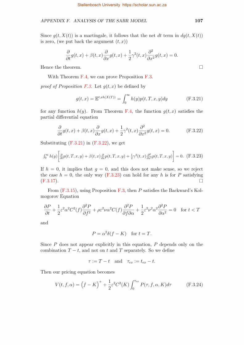
APPENDIX F. ANALYSIS OF THE SABR MODEL 107
Since g(t,X(t)) is a martingale, it follows that the net dt term in dg(t,X(t))is zero, (we put back the argument (t, x))
∂
∂tg(t, x) + β(t, x) ∂
∂xg(t, x) + 1
2γ2(t, x) ∂
2
∂x2 g(t, x) = 0.
Hence the theorem.
With Theorem F.4, we can prove Proposition F.3.
proof of Proposition F.3. Let g(t, x) be defined by
g(t, x) = Et,xh(X(T )) =∫ ∞
0h(y)p(t, T, x, y)dy (F.3.21)
for any function h(y). From Theorem F.4, the function g(t, x) satisfies thepartial differential equation
∂
∂tg(t, x) + β(t, x) ∂
∂xg(t, x) + 1
2γ2(t, x) ∂
2
∂x2 g(t, x) = 0. (F.3.22)
Substituting (F.3.21) in (F.3.22), we get
∫∞0 h(y)
[∂∂tp(t, T, x, y) + β(t, x) ∂
∂xp(t, T, x, y) + 1
2γ2(t, x) ∂2
∂x2p(t, T, x, y)]
= 0. (F.3.23)
If h = 0, it implies that g = 0, and this does not make sense, so we rejectthe case h = 0, the only way (F.3.23) can hold for any h is for P satisfying(F.3.17).
From (F.3.15), using Proposition F.3, then P satisfies the Backward’s Kol-mogorov Equation
∂P
∂t+ 1
2ε2α2C2(f)∂
2P
∂f 2 + ρε2να2C(f) ∂2P
∂f∂α+ 1
2ε2ν2α2∂
2P
∂α2 = 0 for t < T
and
P = α2δ(f −K) for t = T .
Since P does not appear explicitly in this equation, P depends only on thecombination T − t, and not on t and T separately. So we define
τ := T − t and τex := tex − t.
Then our pricing equation becomes
V (t, f, α) =(f −K
)++ 1
2ε2C2(K)
∫ τex
0P (τ, f, α,K)dτ (F.3.24)
Stellenbosch University https://scholar.sun.ac.za

APPENDIX F. ANALYSIS OF THE SABR MODEL 108
where P (τ, f, α;K) is the solution of the problem
∂P
∂τ= 1
2ε2α2C2(f)∂
2P
∂f 2 + ρε2να2C(f) ∂2P
∂f∂α+ 1
2ε2ν2α2∂
2P
∂α2 for τ > 0
P = α2δ(f −K), for τ = 0.(F.3.25)
We solve (F.3.25) to obtain P (τ, f, α;K) and then substitute this solution into(F.3.24) to get the value of V (t, f, α). This yields the price under the SABRmodel. In order to solve (F.3.25), we need to transform it into a heat equationand use the result in equation (G.0.7). Let us make the following change ofvariable
ξ = f −Kε
.
Considering the Taylor expansion of C on ξ, we get
C(f) = C(K + εξ) = C01 + εγ1ξ + 12ε
2γ2ξ2 + · · ·
where
C0 = C(K), γ1 = C ′(K)C(K) γ2 = C ′′(K)
C(K) .
Equation (F.3.25) becomes
∂P
∂τ= 1
2α2C2
01 + 2εγ1ξ + ε2(γ2 + γ21)ξ2 + · · · ∂
2P
∂ξ2 +
ρενα21 + εγ1ξ + 12ε
2γ2ξ2 + · · · ∂
2P
∂ξ∂α+ 1
2ε2ν2α2∂
2P
∂α2 for τ > 0
P = α2δ(εξ) = α2
εδ(ξ) as τ → 0.
(F.3.26)
Expanding P as
Pε(t, ξ, α) = 1εP0(t, ξ, α) + P1(t, ξ, α) + εP2(t, ξ, α) + ε2P3(t, ξ, α) + · · · .
Substituting this expansion into (F.3.26) and equating like powers of ε, leadsto the following O(1
ε) problem:
∂P0
∂τ= 1
2α2C2
0∂2P0
∂ξ2 for τ > 0
P0 = α2δ(ξ) as τ → 0.(F.3.27)
Stellenbosch University https://scholar.sun.ac.za

APPENDIX F. ANALYSIS OF THE SABR MODEL 109
To compute the solution of (F.3.27), we consider the following change of vari-ables
y := ξ
α2 , k = C20
2α2 , t := τ, and u(t, y) := P0(τ, ξ)
The problem in equation (F.3.27) is then reduced to
∂u
∂t− k∂
2u
∂y2 = 0
u(t = 0, y) = δ(y).(F.3.28)
Equation (F.3.28) is the heat or diffusion equation, subject to a Dirac deltain the initial condition. Taking f = 0 in equation (G.0.7), the solution ofequation (F.3.28) is given by
u(t, y) = 1√4πkt
exp(− y2
4kt
).
Turning back to the original variables, we get
P0(τ, ξ) = |α|√2πC2
0τexp
− (f −K)2
2α2C20ξ
2τ
. (F.3.29)
Similarly, like powers of ε leads to the following O(1) problem:
∂P1
∂τ− 1
2α2C2
0∂2P1
∂ξ2 = α2γ1C20ξ∂2P0
∂ξ2 for τ > 0
P1 = 0 as τ → 0,(F.3.30)
whereas the O(ε) problem is given by
∂P2
∂τ− 1
2α2C2
0∂2P2
∂ξ2 = α2γ1C20ξ∂2P1
∂ξ2 + ρνC0∂2P0
∂ξ∂αfor τ > 0
P2 = 0 as τ → 0.(F.3.31)
Substituting (F.3.29) into equation (F.3.30) and making some change of vari-able as we did withO(1
ε) problem, theO(1) problem leads to an inhomogeneous
heat equation which is then solved by equation (G.0.7). We also solve the O(ε)problem in the same way. We do not give the results of these solutions here,because there are not useful. Hence
P = 1εP0 + P1 + εP2 + ε2P3 + · · · = α√
2πC20ε
2τexp
− (f −K)2
2α2C20ε
2τ
+ · · ·
Stellenbosch University https://scholar.sun.ac.za

APPENDIX F. ANALYSIS OF THE SABR MODEL 110
or
P = α√2πC2(K)ε2τ
exp− (f −K)2
2α2C2(K)ε2τ
1 + · · · .
We can write the argument of the exponential of P in form of integral
(f −K)2
2α2C2(K)ε2τ1 + · · · = 1
2τ
(1εα
∫ f
K
dx
C(x)
)2
1 + · · · . (F.3.32)
Hence equation (F.3.32) results. Let us define a new variable z by
z := 1εα
∫ f
K
dx
C(x) .
We havez = 1
ε
J(f)− J(K)α
where J ′(x) = 1/C(x). Moreover, we define B by
B(εαz) := C(f).
We summarise all the results as follows∂
∂f→ 1
εαB(εαz)∂
∂zand ∂
∂α→ ∂
∂α− z
α
∂
∂z
∂2
∂f 2 →1
ε2α2B2(εαz)
∂2
∂z2 − εαB′(εαz)B(εαz)
∂
∂z
∂2
∂f∂α→ 1
εαB(εαz)
∂2
∂z∂α− z
α
∂2
∂z2 −1α
∂
∂z
∂2
∂α2 →∂2
∂α2 −2zα
∂2
∂z∂α+ z2
α2∂2
∂z2 + 2zα2
∂
∂z.
(F.3.33)
We have f −K = εαzC(K), therefore
δ(f −K) = δ(εαzC(K)) = 1εαC(K)δ(z).
Consequently, equation (F.3.24) becomes
V (t, f, α) =(f −K
)++ 1
2ε2C2(K)
∫ τex
0P (τ, z, α)dτ
where P (τ, z, α) is the solution of the following boundary value problem∂P
∂τ= 1
2(1− 2ερνz + ε2ν2z2)∂2P
∂z2 −12εα
B′(εαz)B(εαz)
∂P
∂z
+ (ερν − ε2ν2z)(α∂2P
∂z∂α− ∂P
∂z
)+ 1
2ε2ν2α2∂
2P
∂α2 , for τ > 0
P = α
εC(K)δ(z) as τ → 0.
Stellenbosch University https://scholar.sun.ac.za

APPENDIX F. ANALYSIS OF THE SABR MODEL 111
Let us define P (τ, z, α) by
P (τ, z, α) := ε
αC(K)P.
Consequently, we have
εC(K)α
∂P
∂α= εC(K)
α
∂
∂α
(α
εC(K) P)
= 1αP + ∂P
∂α
εC(K)α
∂2P
∂α2 = εC(K)α
∂2
∂α2
(α
εC(K) P)
= 1α
∂
∂α
(P + α
∂P
∂α
).
It follows that
εC(K)α
∂2P
∂α2 = 1α
∂
∂α
(∂P
∂α+ ∂P
∂α+ α
∂2P
∂α2
)= 2α
∂P
∂α+ ∂2P
∂α2 .
In terms of P , we get
V (t, f, α) =(f −K
)++ 1
2αεC(K)∫ τex
0P (τ, z, α)dτ (F.3.34)
where P is solution of
∂P
∂τ= 1
2(1− 2ερνz + ε2ν2z2)∂2P
∂z2 −12εα
B′(εαz)B(εαz)
∂P
∂z
+ (ερν − ε2ν2z)α ∂2P
∂z∂α+ 1
2ε2ν2
(2α∂P
∂α+ α2∂
2P
∂α2
)for τ > 0
P = δ(z) as τ → 0.
(F.3.35)
Taking all the O(1) terms, we realise that P is the solution of the standarddiffusion problem
∂P
∂τ= 1
2∂2P
∂z2 for τ > 0
P = δ(z) as τ → 0.(F.3.36)
This can be solved using equation (G.0.7). So the solution is a function of zand α. Consequently we can write P as
P (τ, z, α) = P0(τ, z) + εP1(τ, z, α) + ε2P2(τ, z, α) + · · · . (F.3.37)
Stellenbosch University https://scholar.sun.ac.za

APPENDIX F. ANALYSIS OF THE SABR MODEL 112
For this very reason, the derivatives ∂P∂α
, ∂P∂α
and ∂P∂α
are all at least O(ε).Substituting (F.3.37) into (F.3.35), we get
∂P0
∂τ+ ε
∂P1
∂τ+ ε2∂P2
∂τ+ · · · = 1
2(1− 2ερνz + ε2ν2z2)[∂2P0
∂z2 + ε∂2P1
∂z2
+ ε2∂2P2
∂z2 + · · ·]− 1
2εαB′
B
[∂P0
∂z+ ε
∂P1
∂z+ ε2∂P2
∂z+ · · ·
]+ (ερν−
ε2ν2z)α[∂2P0
∂z∂α+ ε
∂2P1
∂z∂α+ ε2 ∂
2P2
∂z∂α+ · · ·
]+ 1
2ε2ν2
2α[∂P0
∂α+ ε
∂P1
∂α
+ ε2∂P2
∂α+ · · ·
]+ α2
[∂2P0
∂α2 + ε∂2P1
∂α2 + ε2∂2P2
∂α2 + · · ·] for τ > 0.
P = δ(z) as τ → 0.
We are only solving for P through O(ε2), therefore, we have
∂P
∂τ= 1
2(1− 2ερνz + ε2ν2z2)∂2P
∂z2 −12εα
B′
B
∂P
∂z+ ερνα
∂2P
∂z∂αfor τ > 0.
P = δ(z) as τ → 0.(F.3.38)
We look for ways to remove the term 12εα
B′
B∂P∂z
in equation (F.3.38). Hence,we introduce a new variable H defined by
P = C(f)C(K)
mH =B(εαz)
B(0)
mH.It follows that
∂P
∂z=B(εαz)
B(0)
m∂H∂z
+ εmαB′(εαz)B(εαz)H
= mεαB′
BP +
(B
B0
)m∂H
∂z.
Also,
∂2P
∂z2 =(B
B0
)m∂2H
∂z2 +2mεαB′
B
(B
B0
)m∂H
∂z
+mε2α2(B
B0
)m×H ×
(mB′2 +B′′B −B′2
B2
).
Lastly, we have
∂2P
∂z∂α=(B(εαz)B(0)
)m[mε
B′
BH +mαε2Hz
B′′
B+ α
B′
B2m(m− 1)ε2zH
+mεαB′
B
∂H
∂α+mεz
B′
B
∂H
∂z+ ∂2H
∂z∂α
].
Stellenbosch University https://scholar.sun.ac.za

APPENDIX F. ANALYSIS OF THE SABR MODEL 113
Hence, taking ε2 → 0, we obtain
∂2P
∂z∂α=B(εαz)
B(0)
m ∂2H
∂z∂α+ εmz
B′
B
∂H
∂z+ εmα
B′
B
∂H
∂α+ εm
B′
BH +O(ε2)
.Consequently, the price option in equation (F.3.34) is now given by
V (t, f, α) =(f −K
)++ 1
2αεB(0)B(εαz)
B(0)
m ∫ τex
0H(τ, z, α)dτ. (F.3.39)
Substituting these results in equation (F.3.38), ignoring all the O(ε3) termsand doing some elementary calculation, we get
∂H
∂τ= 1
2(1− 2ερνz + ε2ν2z2)∂2H
∂z2 + εα
(m− 1
2
)B′
B
∂H
∂z
+ 12ε
2α2[mB′′
B+ (m2 − 2m)B
′2
B2
]H − ε2mρνα
B′
B
(z∂H
∂z−H
)
+ ερνα
∂2H
∂z∂α+ εmα
B′
B
∂H
∂α
.We take m = 1
2 to cancel the term B′
B∂H∂z
, consequently our option price is now
V (t, f, α) =(f −K
)++ 1
2αεB(0)B(εαz)
B(0)
12 ∫ τex
0H(τ, z, α)dτ (F.3.40)
where H(τ, z, α) is the solution of
∂H
∂τ= 1
2(1− 2ερνz + ε2ν2z2)∂2H
∂z2 + ε2α2[
14B′′
B− 3
8B′2
B2
]H
− 12ε
2ρναB′
B
(z∂H
∂z−H
)+ ερνα
∂2H
∂z∂α+ ε
12α
B′
B
∂H
∂α
. (F.3.41)
for τ > 0, with initial condition H = δ(z) at τ = 0. Taking all the O(1) terms,we have the following problem
∂H
∂τ= 1
2∂2H
∂z2
H = δ(z).
This is an heat equation and can be solved using equation (G.0.7). The solutionH0 = H0(z, τ). Therefore, we can expand H as
H(τ, z, α) = H0(τ, z) + εH1(τ, z, α) + ε2H2(τ, z, α) + · · · . (F.3.42)
Stellenbosch University https://scholar.sun.ac.za

APPENDIX F. ANALYSIS OF THE SABR MODEL 114
Substituting (F.3.42) into (F.3.41), we get
∂H0
∂τ+ ε
∂H1
∂τ+ ε2∂H2
∂τ+ · · · = 1
2(1− 2ερνz + ε2ν2z2)[∂2H0
∂z2 + ε∂2H1
∂z2 +
ε2∂2H2
∂z2 + · · ·]
+ ε2α2[
14B′′
B− 3
8B′2
B2
](H0 + εH1 + ε2H2 + · · ·
)
− 12ε
2ρναB′
B
[z
(∂H0
∂z+ ε
∂H1
∂z+ ε2∂H2
∂z+ · · ·
)−(H0 + εH1 + · · ·
)]
+ ερνα
(∂2H0
∂z∂α+ ε
∂2H1
∂z∂α+ · · ·
)+ ε
12α
B′
B
(∂H0
∂α+ ε
∂H1
∂α+ · · ·
).The fact that H0 is independent of α and ignoring all the O(ε3) terms, we
note the following ∂2H0∂z∂α
= 0, ∂H0∂α
= 0, ε2(z ∂
2H0∂z−H0
)= ε2
(z ∂
2H∂z−H
), and
ε2H0 = ε2H. Considering all the O(ε) terms, we have
∂H1
∂τ= 1
2∂2H1
∂z2 − ρνz∂2H0
∂z2 .
for τ > 0, with initial condition H = δ(z) at τ = 0. This is an heat equa-tion and can be solved using formula (G.0.7). The solution H1 = H1(z, τ).Likewise, we prove that H2 = H2(z, τ) and so on. Therefore, H = H(z, τ).Consequently equation (F.3.41) is reduced to
∂H
∂τ= 1
2(1− 2ερνz + ε2ν2z2)∂2H
∂z2 + ε2α2[
14B′′
B+ 3
8B′2
B2
]H
− 12ε
2ρναB′
B
(z∂H
∂z−H
) (F.3.43)
for τ > 0, with initial condition H = δ(z) at τ = 0. For any fixed z0
B′(εαz)B(εαz) = B′(εαz0)
B(εαz0) +O(ε) and B′′(εαz)B(εαz) = B′′(εαz0)
B(εαz0) +O(ε).
So up to and including O(ε2), B′/B and B′′/B can be replaced by any constantevaluated at any convenient z0. Therefore we can define the following
b1 := B′(εαz0)B(εαz0) and b2 := B′′(εαz0)
B(εαz0) .
Let us define a new variable H by
H = exp(1
4ε2ρναb1z
2)H.
Stellenbosch University https://scholar.sun.ac.za

APPENDIX F. ANALYSIS OF THE SABR MODEL 115
It follows that
∂H
∂τ= exp
(14ε
2ρναb1z2)∂H
∂τ
and
∂H
∂z= exp
(14ε
2ρναb1z2)∂H
∂z+ 1
2ε2ρναb1zH
.Moreover
∂2H
∂z2 = 12ε
2ρναb1z × exp(1
4ε2ρναb1z
2)×
∂H∂z
+ 12ε
2ρναb1zH
+ exp
(14ε
2ρναb1z2)[∂2H
∂z2 + 12ε
2ρναb1H + 12ε
2ρναb1z∂H
∂z
].
Ignoring the O(ε4) term, we have
∂2H
∂z2 = exp(1
4ε2ρναb1z
2)∂2H
∂z2 + ε2ρναb1z∂H
∂z+ 1
2ε2ρναb1H
.Consequently, our option price (F.3.40) becomes
V (t, f, α) =(f −K
)++ 1
2αε√B(0)B(εαz)eε2ρναb1z2/4
∫ τex
0H(τ, z, α)dτ.
In addition, substituting these results in equation (F.3.43) and ignoring all theO(ε3) term, we have
∂H
∂τ= 1
2(1− 2ερνz + ε2ν2z2
)∂2H
∂z2 + 34ε
2ρναb1H + ε2α2[
14b2 −
38b
21
]H
for τ > 0, with initial condition H = δ(z) at τ = 0. Afterwards, we define
x := 1εν
∫ ενz
0
dt√1− 2ρt+ t2
.
We compute the integral J and then substitute the limits to get x.
J :=∫ dt√
1− 2ρt+ t2=∫ dt√
1− ρ2√
1 + (t−ρ)2
1−ρ2
.
We perform a change of variable twice, we define
t− ρ√1− ρ2 = u and u = tan θ.
Stellenbosch University https://scholar.sun.ac.za

APPENDIX F. ANALYSIS OF THE SABR MODEL 116
It follows that
J =∫ dθ
cos2 θ√
1 + tan2 θ=∫ cos θdθ
cos2 θ=∫ cos θdθ
1− sin2 θ== 1
2 log∣∣∣∣∣1 + sin θ1− sin θ
∣∣∣∣∣.Going back to the old variables above, and since
sin θ = tan θ√1 + tan2 θ
and u2 + 1 = 1 + t2 − 2ρt1− ρ2 ,
we have
J = 12 log
t−ρ√1−ρ2
+√
1+t2−2ρt√1−ρ2
√1+t2−2ρt√
1−ρ2− t−ρ√
1−ρ2
= 12 log
(√
1 + t2 − 2ρt+ (t− ρ))2
1 + t2 − 2ρt− (t2 − 2ρt+ ρ2)
.
It follows
x = 1εν
log√1 + t2 − 2ρt+ t− ρ√
1− ρ2
ενz0
= 1εν
log√1− ρ2 + y2 + y
1− ρ
.where y is given by
y := ενz − ρ.For ρ 6= 1 we have,
(1− ρ)e2ενx − 2yeενx = 1 + ρ =⇒ y = 12[(eενx − e−ενx)− ρ(eενx + e−ενx)
].
Therefore
y = sinh(ενx)− ρ cosh(ενx) =⇒ ενz = sinh(ενx)− ρ(
cosh(ενx)− 1).
After the transformation form z to x, we have
∂H
∂z= ∂x
∂z
∂H
∂x= 1√
1− 2ερνz + ε2ν2z2∂H
∂x= 1I(ενz)
∂H
∂x.
Also
∂2H
∂z2 = −εν I′
I2∂H
∂x+ 1I2∂2H
∂x2 .
where, I is defined byI(t) =
√1− 2ρt+ t2.
In terms of x, we have
V (t, f, α) =(f −K
)++ 1
2αε√B(0)B(εαz)eε2ρναb1z2/4
∫ τex
0H(τ, x)dτ
Stellenbosch University https://scholar.sun.ac.za

APPENDIX F. ANALYSIS OF THE SABR MODEL 117
and
∂H
∂τ= 1
2∂2H
∂x2 −12ενI
′(ενz)∂H∂x
+ 34ε
2ρναb1H + ε2α2[
14b2 −
38b
21
]H
for τ > 0, with initial condition H = δ(x) at τ = 0. Lastly, we define Q(τ, x)by
H = I12(ενz(x)
)Q =
(1− 2ερνz + ε2ν2z2
) 14Q.
It follows
∂H
∂τ= I
12(ενz
)∂Q∂τ
and ∂H
∂x= Q
∂z
∂x
∂I12
∂z+ I
12∂Q
∂x.
Finally
∂2H
∂x2 = ∂
∂x
(∂H
∂x
)= ∂z
∂x
12ενI
′I−12
∂Q∂x
+ 12ενI
′(ενz)Q
+ I12(ενz
)∂2Q
∂x2 + 12εν
(ενI
∂2I
∂z2Q+ I ′(ενz)∂Q∂x
).Consequently, our option price is now
V (t, f, α) =(f −K
)++ 1
2αε√B(0)B(εαz)I 1
2(ενz
)e
14 ε
2ρναb1z2∫ τex
0Q(τ, x)dτ
with Q solution of
∂Q
∂τ= 1
2∂2Q
∂x2 + ε2ν2(
14I′′I − 1
8I′2)Q+ 3
4ε2ρναb1Q+ ε2α2
[14b2 −
38b
21
]Q
for τ > 0, with initial condition Q = δ(x) at τ = 0. We can substitute I(ενz),I ′(ενz), I ′′(ενz) by the constants I(ενz0), I ′(ενz0), I ′′(ενz0) and commit onlyO(ε) errors. We will choose z0 later on. We define the constant κ by
κ = ν2(
14I′′(ενz0)I(ενz0)− 1
8[I ′(ενz0)
]2)+ 3
4ρναb1 + α2[
14b2 −
38b
21
].
Therefore through O(ε2), we can simplify our problem to
∂Q
∂τ= 1
2∂2Q
∂x2 + ε2κQ for τ > 0,
Q = δ(x) at τ = 0.
This is an heat equation and can be solved using (G.0.7). The solution is
Q(τ, x) = 1√2πτ
e−x22τ eε
2κτ .
Stellenbosch University https://scholar.sun.ac.za

APPENDIX F. ANALYSIS OF THE SABR MODEL 118
We observe that the Taylor series of eε2κτ at ε = 0 is the same as the Taylorseries of 1
(1− 22κε
2τ+··· )32at ε = 0. Hence, trough (ε2), we have
Q(τ, x) = 1√2πτ
e−x22τ
1(1− 2
3κε2τ + · · ·
) 32.
The option price is given by
V (t, f, α) =(f −K
)++ 1
2f −Kx
∫ τex
0
1√2πτ
e−x22τ eε
2θeε2κτdτ, (F.3.44)
where we have defined ε2θ by
ε2θ := log εαz
f −K
√B(0)B(εαz)
+ logxI 1
2 (ενz)z
+ 14ε
2ρναb1z2.
Expanding ε2θ trough ε2 yields
ε2θ ∼
112b2 −
18b
21
)ε2α2z2 +
112I ′′(1
2ενz)I(1
2ενz) −124
I ′(12ενz)
I0(12ενz)
2ε2ν2z2
+ 14ε
2ρναb1z2.
Using the factz
x= 1 +O(ε) and I(ενz) = 1 + · · · ,
we note that θx2 matches
κ
3 = 13ν
2(
14I′′(ενz0)I(ενz0)− 1
8[I ′(ενz0)
]2)+ 1
4ρναb1 + 13α
2[
14b2 −
38b
21
]
and therefore
eε2κτ = 1(
1− 23κε
2τ + · · ·) 3
2= 1(
1− 2ε2τ θx2
) 32
+O(ε4)
trough O(ε2). Hence, our option price becomes
V (t, f, α) =(f −K
)++ 1
2f −Kx
∫ τex
0
1√2πτ
e−x22τ eε
2θ 1(1− 2ε2τ θ
x2
) 32dτ.
Changing integration variables to q := x2
2τ , we get
V (t, f, α) =(f −K
)++
∣∣∣f −K∣∣∣4√π
∫ ∞x2
2τex
e−q+ε2θ(
q − ε2θ) 3
2dq.
Stellenbosch University https://scholar.sun.ac.za

APPENDIX F. ANALYSIS OF THE SABR MODEL 119
It follows that, the value of a European call option is given by
V (t, f, α) =(f −K
)++
∣∣∣f −K∣∣∣4√π
∫ ∞x2
2τex−ε2θ
q−32 e−qdq, (F.3.45)
with5
ε2θ = log εαz
f −K
√B(0)B(εαz)
+ logxI 1
2 (ενz)z
+ 14ε
2ρναb1z2
trough O(ε2).
5This is found in (Hagan et al., 2002).
Stellenbosch University https://scholar.sun.ac.za

Appendix G
Fourier transform
We give some useful formulae for the Fourier transform, which provide powerfultools to solve the heat equation. Here, for a given complex function f , fdenotes its complex conjugate.
G.0.1 Definitions and elementary proprietiesDefinition G.1 (Fourier transform on L1). If u ∈ L1(Rn), we define itsFourier transform
u(y) := 1(2π)n/2
∫Rne−ix.yu(x)dx (y ∈ Rn) (G.0.1)
and its inverse Fourier transform
u`(y) := 1(2π)n/2
∫Rneix.yu(x)dx (y ∈ Rn) (G.0.2)
Theorem G.2 (Proprieties of Fourier transform). Assume u, v ∈ L2(Rn).Then ∫
Rnuvdx =
∫Rnuvdy; (G.0.3)
Dαu = (iy)αu for each multiindex α such that Dαu ∈ L2(Rn); (G.0.4)
ˆ(u ∗ v) = (2π)n/2uv; (G.0.5)
u = u`. (G.0.6)
120
Stellenbosch University https://scholar.sun.ac.za

APPENDIX G. FOURIER TRANSFORM 121
G.0.2 Inhomogeneous Heat Equation by Fouriertransform
We consider the initial value problem for u = u(x, t), u ∈ C∞(Rn ×R+),
ut −∆u = f(x, t) in x ∈ Rn, t ≥ 0,u(x, 0) = φ(x),
where φ and f are given. By Fourier transform, we have
ut −∆u = f(x, t)
u(x, 0) = φ(x).
We obtain an initial value problem for an ordinary differential equation:
du
dt+ |ξ|2u = f(ξ, t)
u(ξ, 0) = φ(ξ).
The solution is given by
u(ξ, t) = e−|ξ|2tφ(ξ) +
∫ t
0e−|ξ|
2(t−τ)f(ξ, t)dτ.
Using the inverse Fourier transform, we have
u(x, t) = 1(2π)n/2
∫Rneix.ξ
(e−|ξ|
2tφ(ξ) +∫ t
0e−|ξ|
2(t−τ)f(ξ, t)dτ)dξ.
After calculation, we have
u(x, t) = 1(2√πt)n
∫Rnφ(y)e−|x−y|2/4tdy
+∫ t
0
∫Rn
1(2√π(t− τ)
)nf(y, τ)e−|x−y|2/4(t−τ)dydτ. (G.0.7)
Stellenbosch University https://scholar.sun.ac.za

Appendix H
Computer code
In this appendix, we give a summary of some the computer codes. Shouldyou have questions or concerns regarding codes, please feel free to drop me amessage or email at [email protected] or [email protected].
H.1 SABR modelIt is here where we give a summary of the steps taken to implement the SABRmodel. This rather a user guide which could be used in conjunction with thecode to understand our implementation. The implementation was done inMatlab. We use functions written by of Fabrice Douglas Rouah (availableat http://www.volopta.com).
This function estimates all the parameters simultaneously using Method 1
function y = EstimateAllParameters(params,MktStrike,MktVol,F,T,b)% ---------------------------------------------------------------% Returns the following SABR parameters:% a = alpha% r = rho% v = vol-of-vol% Required inputs:% MktStrike = Vector of Strikes% MktVol = Vector of corresponding volatilities% F = spot price% T = maturity% b = beta parameter% --------------------------------------------------------------a = params(1);r = params(2);v = params(3);N = length(MktVol);% Define the model volatility and the squared error terms
122
Stellenbosch University https://scholar.sun.ac.za

APPENDIX H. COMPUTER CODE 123
for i=1:NModelVol(i) = SABRvol(a,b,r,v,F,MktStrike(i),T);error(i) = (ModelVol(i) - MktVol(i))^2;end;% Return the SSEy = sum(error);% Impose the constraint that -1 <= rho <= +1 and that v>0if abs(r)>1 | v<0y = 1e100;end
This function estimates all the parameters simultaneously using Method 2
function y = EstimateAllParametersFine_Tune(params,MktStrike,MktVol,F,T,b,FineTune)
% ------------------------------------------------------% Uses the Fine Tuned version of the SABR volatilities.% Returns the following SABR parameters:% a = alpha% r = rho% v = vol-of-vol% Required inputs:% MktStrike = Vector of Strikes% MktVol = Vector of corresponding volatilities% F = spot price% T = maturity% b = beta parameter% FineTune? (’Y’ or ’N’)% ---------------------------------------------------a = params(1);r = params(2);v = params(3);N = length(MktVol);% Define the model volatility and the squared error termsfor i=1:NModelVol(i) = SABRvol_FineTune(a,b,r,v,F,MktStrike(i),T,FineTune);error(i) = (ModelVol(i) - MktVol(i))^2;end;% Return the SSEy = sum(error);% Impose the constraint that -1 <= rho <= +1 and that v>0if abs(r)>1 | v<0y = 1e100;end
Stellenbosch University https://scholar.sun.ac.za

APPENDIX H. COMPUTER CODE 124
This function estimates the parameters ρ and ν simultaneously using Method1
function y = EstimateRhoAndVol(params,MktStrike,MktVol,ATMVol,F,T,b)% ------------------------------------------------% Returns the following SABR parameters:% r = rho% v = vol-of-vol% Uses ATM volatility to estimate alpha% Required inputs:% MktStrike = Vector of Strikes% MktVol = Vector of corresponding volatilities% ATMVol = ATM volatility% F = spot price% T = maturity% b = beta parameter% ------------------------------------------------r = params(1);v = params(2);a = findAlpha(F,F,T,ATMVol,b,r,v);N = length(MktVol);% Define the model volatility and the squared error termsfor i=1:NModelVol(i) = SABRvol(a,b,r,v,F,MktStrike(i),T);error(i) = (ModelVol(i) - MktVol(i))^2;end;% Return the SSEy = sum(error);% Impose the constraint that -1 <= rho <= +1 and that v>0% via a penalty on the objective functionif abs(r)>1 | v<0y = 1e100;end
This function estimates the parameters ρ and ν simultaneously using Method2
function y = EstimateRhoAndVol(params,MktStrike,MktVol,ATMVol,F,T,b,FineTune)
% --------------------------------------------% Uses the Fine Tuned version of the SABR volatilities.% Returns the following SABR parameters:% r = rho% v = vol-of-vol% Uses ATM volatility to estimate alpha
Stellenbosch University https://scholar.sun.ac.za
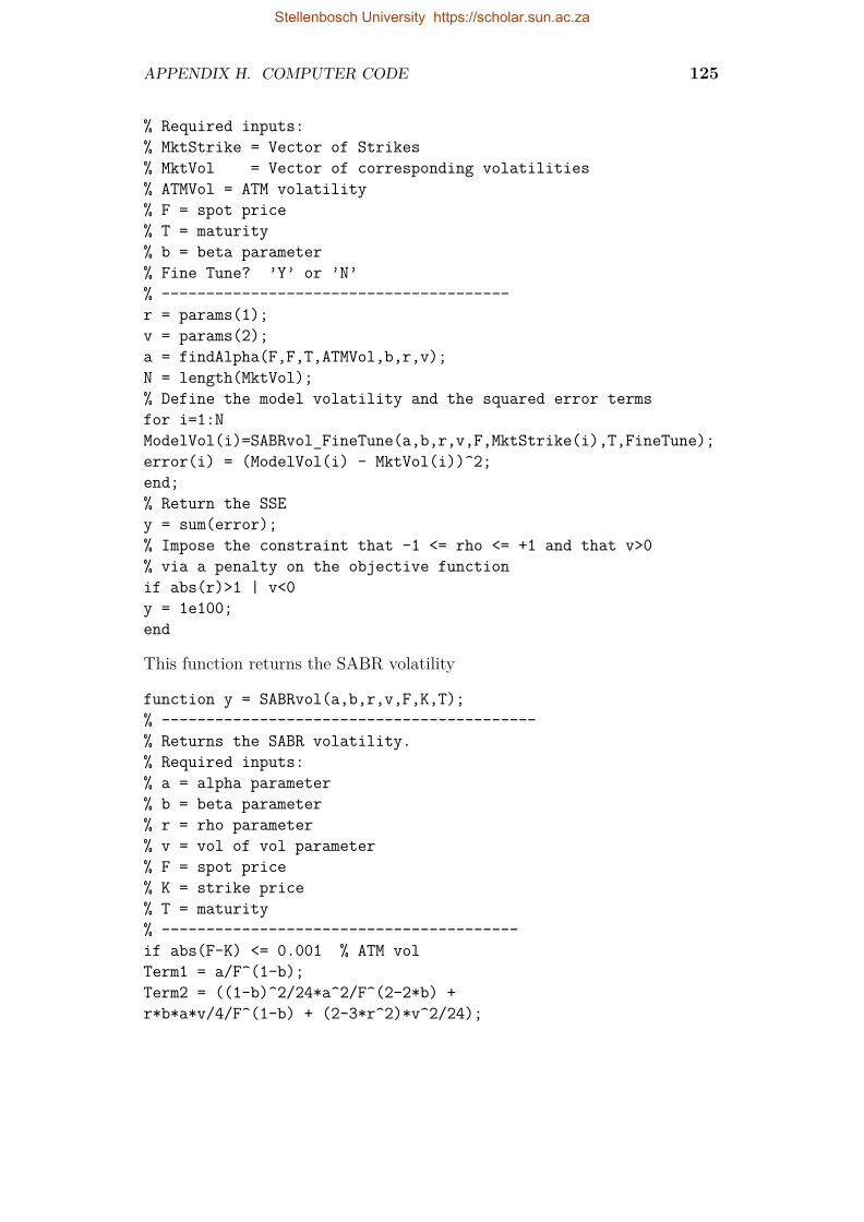
APPENDIX H. COMPUTER CODE 125
% Required inputs:% MktStrike = Vector of Strikes% MktVol = Vector of corresponding volatilities% ATMVol = ATM volatility% F = spot price% T = maturity% b = beta parameter% Fine Tune? ’Y’ or ’N’% ---------------------------------------r = params(1);v = params(2);a = findAlpha(F,F,T,ATMVol,b,r,v);N = length(MktVol);% Define the model volatility and the squared error termsfor i=1:NModelVol(i)=SABRvol_FineTune(a,b,r,v,F,MktStrike(i),T,FineTune);error(i) = (ModelVol(i) - MktVol(i))^2;end;% Return the SSEy = sum(error);% Impose the constraint that -1 <= rho <= +1 and that v>0% via a penalty on the objective functionif abs(r)>1 | v<0y = 1e100;end
This function returns the SABR volatility
function y = SABRvol(a,b,r,v,F,K,T);% ------------------------------------------% Returns the SABR volatility.% Required inputs:% a = alpha parameter% b = beta parameter% r = rho parameter% v = vol of vol parameter% F = spot price% K = strike price% T = maturity% ----------------------------------------if abs(F-K) <= 0.001 % ATM volTerm1 = a/F^(1-b);Term2 = ((1-b)^2/24*a^2/F^(2-2*b) +r*b*a*v/4/F^(1-b) + (2-3*r^2)*v^2/24);
Stellenbosch University https://scholar.sun.ac.za

APPENDIX H. COMPUTER CODE 126
y = Term1*(1 + Term2*T);else % Non-ATM volFK = F*K;z = v/a*(FK)^((1-b)/2)*log(F/K);x = log((sqrt(1 - 2*r*z + z^2) + z - r)/(1-r));Term1 = a / FK^((1-b)/2) / (1 + (1-b)^2/24*log(F/K)^2 +(1-b)^4/1920*log(F/K)^4);
if abs(x-z) < 1e-10Term2 = 1;elseTerm2 = z / x;endTerm3 = 1 + ((1-b)^2/24*a^2/FK^(1-b) + r*b*v*a/4/FK^((1-b)/2) +(2-3*r^2)/24*v^2)*T;
y = Term1*Term2*Term3;end
This function returns the SABR volatility using Method 2
function y = SABRvol_FineTune(a,b,r,v,F,K,T,FineTune);% -----------------------------------------% Returns two possible SABR volatilities.% (1) Original SABR formula by Hagan et al.% (2) Fine Tuned formula summarized in% "Fine-Tune Your Smile" by Jan Obloj% Required inputs:% a = alpha parameter% b = beta parameter% r = rho parameter% v = vol of vol parameter% F = spot price% K = strike price% T = maturity% FineTune? (’Y’ or ’N’)% ---------------------------------------------x = log(F/K);% Separate out into cases x=0, b=1, and b<1.if abs(x) <= 0.0001I0H = a*K^(b-1);I0B = a*K^(b-1);elseif abs(v) <= 0.001 % ATM volI0H = x*a*(1-b) / (F^(1-b)-K^(1-b));I0B = x*a*(1-b) / (F^(1-b)-K^(1-b));
Stellenbosch University https://scholar.sun.ac.za
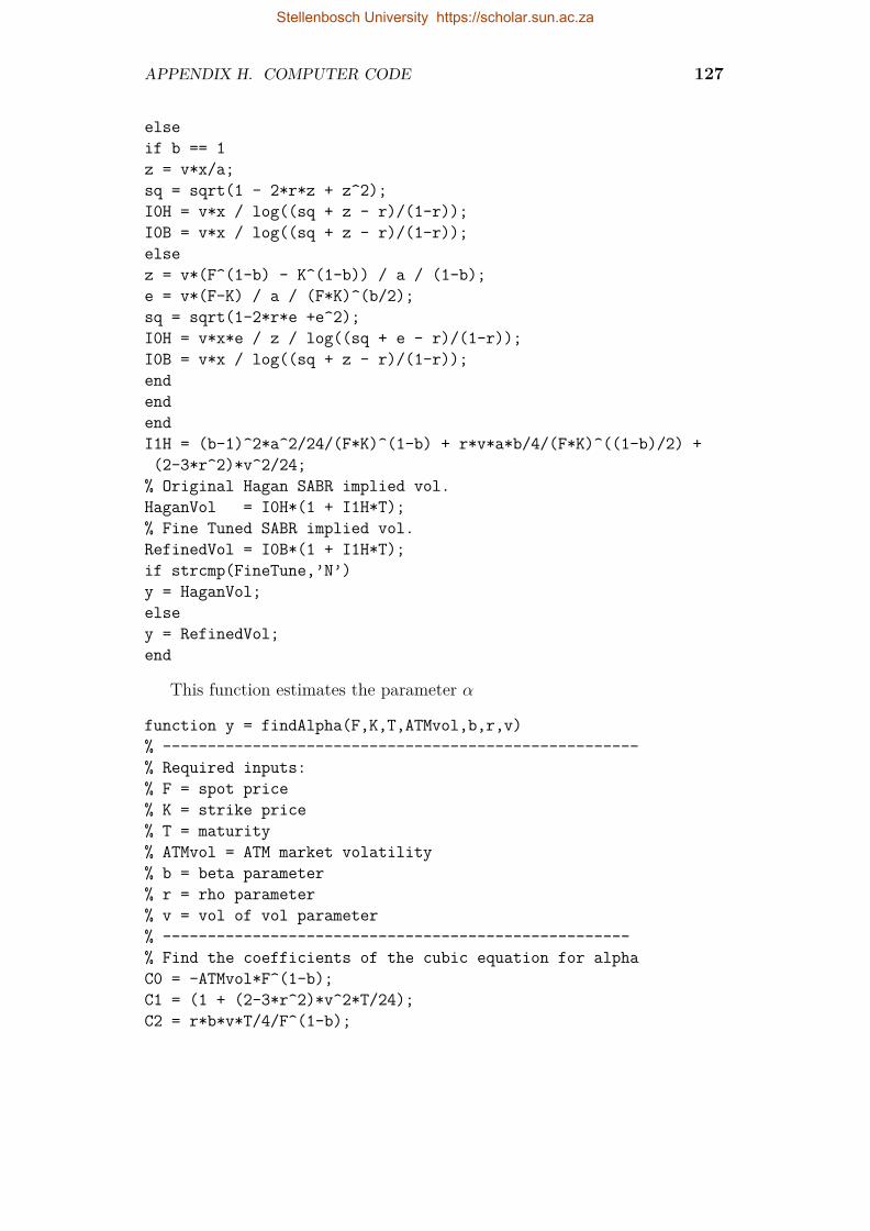
APPENDIX H. COMPUTER CODE 127
elseif b == 1z = v*x/a;sq = sqrt(1 - 2*r*z + z^2);I0H = v*x / log((sq + z - r)/(1-r));I0B = v*x / log((sq + z - r)/(1-r));elsez = v*(F^(1-b) - K^(1-b)) / a / (1-b);e = v*(F-K) / a / (F*K)^(b/2);sq = sqrt(1-2*r*e +e^2);I0H = v*x*e / z / log((sq + e - r)/(1-r));I0B = v*x / log((sq + z - r)/(1-r));endendendI1H = (b-1)^2*a^2/24/(F*K)^(1-b) + r*v*a*b/4/(F*K)^((1-b)/2) +(2-3*r^2)*v^2/24;
% Original Hagan SABR implied vol.HaganVol = I0H*(1 + I1H*T);% Fine Tuned SABR implied vol.RefinedVol = I0B*(1 + I1H*T);if strcmp(FineTune,’N’)y = HaganVol;elsey = RefinedVol;end
This function estimates the parameter α
function y = findAlpha(F,K,T,ATMvol,b,r,v)% -----------------------------------------------------% Required inputs:% F = spot price% K = strike price% T = maturity% ATMvol = ATM market volatility% b = beta parameter% r = rho parameter% v = vol of vol parameter% ----------------------------------------------------% Find the coefficients of the cubic equation for alphaC0 = -ATMvol*F^(1-b);C1 = (1 + (2-3*r^2)*v^2*T/24);C2 = r*b*v*T/4/F^(1-b);
Stellenbosch University https://scholar.sun.ac.za

APPENDIX H. COMPUTER CODE 128
C3 = (1-b)^2*T/24/F^(2-2*b);% Return the roots of the cubic equation (multiple roots)AlphaVector = roots([C3 C2 C1 C0]);% Find and return the smallest positive rootindex = find(AlphaVector>0);Alpha = AlphaVector(index);y = min(Alpha);
This a short section from the code for calibrating a 5Y12Y swaption, given theabove functions.
%% Calibrating the smile for a 5Y12Y swaption%Define the starting values and options for fminsearchstart = [0.3,0.3];options = optimset(’MaxFunEvals’, 1e5, ’TolFun’,1e-8, ’TolX’, 1e-10);% Parameter estimation method 1. Set Beta = 0.5.% Estimate rho and v, and at each iteration step,% Find alpha as the cubic root using the findAlpha functionBeta = 0.5;[param, feval] = fminsearch(@(par)EstimateRhoAndVol(par,K12Y,Vol5Y(:,8),Vol12ATM(8),Swapcurve(12),Expiry(8)/12,Beta), start,options);R1 = param(1);V1 = param(2);A1 = findAlpha(Swapcurve(12),Swapcurve(12),Expiry(8)/12,Vol12ATM(8), Beta,R1,V1);for j=1:length(K12Y);
SABRVol5Y12Y_method1(j) = SABRvol(A1,Beta,R1,V1,Swapcurve(12), K12Y(j),Expiry(8)/12);
end
% Parameter estimation method 2. Set beta = 0.5.% Estimate rho, v, and alpha directlyBeta = 0.5;start = [0.3,0.3,0.3];[params, feval] = fminsearch(@(par)EstimateAllParameters(par,K12Y, Vol5Y(:,8), Swapcurve(12),Expiry(8)/12,Beta),start, options);A2 = params(1);R2 = params(2);V2 = params(3);for j=1:length(K12Y);
SABRVol5Y12Y_method2(j)=SABRvol(A2,Beta,R2,V2,Swapcurve(12),
Stellenbosch University https://scholar.sun.ac.za

APPENDIX H. COMPUTER CODE 129
K12Y(j),Expiry(8)/12);end
% Fined Tuned parameter estimation method 1.Beta = 0.5;start = [0.3,0.3];FineTune = ’Y’;[param1F, feval] = fminsearch(@(par)EstimateRhoAndVol_FineTune(par,K12Y,Vol5Y(:,8), Vol12ATM(8),Swapcurve(12),Expiry(8)/12,Beta,FineTune), start, options);R1F = param1F(1);V1F = param1F(2);A1F = findAlpha(Swapcurve(12),Swapcurve(12),Expiry(8)/12,Vol12ATM(8),Beta,R1F,V1F);for j=1:length(K12Y);
SABRVol5Y12Y_method1FINE(j) = SABRvol(A1F,Beta,R1F,V1F,Swapcurve(12),K12Y(j),Expiry(8)/12);
end
% Fined Tuned parameter estimation method 2.Beta = 0.5;start = [0.3,0.3,0.3];FineTune = ’Y’;[param2F, feval]=fminsearch(@(par)EstimateAllParameters_FineTune(par,K12Y,Vol5Y(:,8),Swapcurve(12),Expiry(8)/12,Beta,FineTune),start, options);A2F = param2F(1);R2F = param2F(2);V2F = param2F(3);for j=1:length(K12Y);
SABRVol5Y12Y_method2FINE(j) = SABRvol(A2F,Beta,R2F,V2F,Swapcurve(12),K12Y(j),Expiry(8)/12);
end
H.2 Yield curves via QuantlibIt is here where we give a summary of the steps taken to implement the yieldcurves in C++ language via the Quantlib framework. The full code can befound at Mbongo (2014).
H.2.1 Eonia yield curveReal eoniaquotes[] =.......
Stellenbosch University https://scholar.sun.ac.za

APPENDIX H. COMPUTER CODE 130
boost::shared_ptr<RateHelper> rhon =boost::make_shared<DepositRateHelper>(eoniaquotes[0], 1 * Days,0, TARGET(), Following, false, Actual360());
boost::shared_ptr<OvernightIndex> eoniaBt =boost::make_shared<Eonia>();
boost::shared_ptr<RateHelper> rhe1w =boost::make_shared<OISRateHelper>(2, 1 * Weeks, Handle<Quote>(boost::make_shared<SimpleQuote>(eoniaquotes[1])), eoniaBt);boost::shared_ptr<RateHelper> rhe30y =boost::make_shared<OISRateHelper>(2, 30 * Years, Handle<Quote>(boost::make_shared<SimpleQuote>(eoniaquotes[33])),eoniaBt);boost::shared_ptr<RateHelper> rhefeb13 =boost::make_shared<DatedOISRateHelper>(Date(16, January, 2013), Date(13, February, 2013),Handle<Quote>(boost::make_shared<SimpleQuote>(eoniaquotes[34])),eoniaBt);
std::vector<boost::shared_ptr<RateHelper> > eoniaratehelpers;eoniaratehelpers += rhon, rhe1w,..., rhe1m,rhefeb13, rhemar13, rheapr13, rhemay13, rhejun13, rhejul13,/*rhe2m,..., rhe7m,*/ // replaced by forwardsrhe8m,..., rhe21m, rhe2y,..., rhe30y;
PiecewiseYieldCurve<Discount, LogLinear> curve(0, TARGET(),eoniaratehelpers, Actual365Fixed(), tolerance);curve.recalculate();std::vector<Rate> spotRates, discountFactors, forwardRates;
Period forwardTenor(3, Months); // 3 months forward// Construct spot curve, forward curve and discount curvefor(Size i=0;i<eoniaratehelpers.size();i++) Rate rate;Date d = eoniaratehelpers[i]->latestDate();// spot raterate=curve.zeroRate(d,Actual365Fixed(),Continuous,Annual,true);spotRates.push_back(rate);
// forward raterate = curve.forwardRate(d, TARGET().advance(d, forwardTenor),dayCounterOIS, Simple, Annual, true);forwardRates.push_back(rate);
// discount raterate = curve.discount(d, true);
Stellenbosch University https://scholar.sun.ac.za

APPENDIX H. COMPUTER CODE 131
discountFactors.push_back(rate);
If we insert the forwards, we have to remove the swaps with the samematurity, or the curve will complain. For instance, if we use EONECBFEB13,remove the 2-months spot.
Building the Euribor3M yield curve with the Eoniacurve as discount
MARKET DATA
// depositsRate dONDQuote=...,..., d1wQuote=..., ..., d12mQuote=...;
// FRAs Underlying Euribor3M, Euribor6M, Euribor12MRate Tod3MQuote=...,..., fra6x9Quote=...; Tom6MQuote=...,...,fra18x24Quote=...; fra12x24Quote=...;
// FRAs Underlying Euribor6M(IMM)Real IMMF3FRAQuote=...,...,IMMJ3FRAQuote=...;
// futures Underlying Euribor3MReal FUT3MZ2Quote=..., FUT3MF3Quote=..., FUT3MG3Quote=...,FUT3MH3Quote=..., FUT3MM3Quote=..., FUT3MU3Quote=...;
// EUR IRS on Euribor3MRate AB3E1YQuote=..., AB3E15MQuote=..., ....AB3E60YQuote=...;
We need to build an OIS discount curve that, we will use to bootstrap aforward curve (this was done in H.2.1).
boost::shared_ptr<YieldTermStructure> oisDiscountCurve(new PiecewiseYieldCurve<Discount,LogLinear>(settlementDate, eoniaratehelpers, termStructureDayCounter,
tolerance));
QUOTES// depositsboost::shared_ptr<Quote> dONDRate(new SimpleQuote(dONDQuote));boost::shared_ptr<Quote> d1wRate(new SimpleQuote(d1wQuote));boost::shared_ptr<Quote> d12mRate(new SimpleQuote(d2mQuote));
// FRAs Underlying Euribor3M, Euribor6M, Euribor12Mboost::shared_ptr<Quote>Tod3MRate(new SimpleQuote(Tod3MQuote));boost::shared_ptr<Quote>fra6x9Rate(new SimpleQuote(fra6x9Quote));boost::shared_ptr<Quote>fra18x24Rate(new SimpleQuote(fra18x24Quote));boost::shared_ptr<Quote>
Stellenbosch University https://scholar.sun.ac.za

APPENDIX H. COMPUTER CODE 132
fra12x24Rate(new SimpleQuote(fra12x24Quote));
// FRAs Underlying Euribor3M(IMM)boost::shared_ptr<Quote>IMMF3FRAPrice(new SimpleQuote(IMMF3FRAQuote));
// Futuresboost::shared_ptr<Quote>FUT3MZ2Price(new SimpleQuote(FUT3MZ2Quote));
// EUR IRS on Euribor3Mboost::shared_ptr<Quote>AB3E1YRate(new SimpleQuote(AB3E1YQuote));boost::shared_ptr<Quote>AB3E50YRate(new SimpleQuote(AB3E50YQuote));
RATE HELPERS// RateHelpers are built from the above quotes together with// other instrument dependant infos. Quotes are passed in// relinkable handles which could be relinked to some other// data source later.
boost::shared_ptr<RateHelper> d3w(new DepositRateHelper(Handle<Quote>(d3wRate), 3*Weeks, fixingDays,calendar, Following, false, depositDayCounter));// FRAs Underlying Euribor3M, Euribor6M, Euribor12M
boost::shared_ptr<RateHelper> fra1x4(new FraRateHelper(Handle<Quote>(fra1x4Rate),1, 4, fixingDays, calendar, ModifiedFollowing,true, depositDayCounter));
boost::shared_ptr<RateHelper> fra2x8(new FraRateHelper(Handle<Quote>(fra2x8Rate),2, 8, fixingDays, calendar, ModifiedFollowing,true, depositDayCounter));
boost::shared_ptr<RateHelper> fra12x24(new FraRateHelper(Handle<Quote>(fra12x24Rate),12, 24, fixingDays, calendar, ModifiedFollowing,true, depositDayCounter));
// setup FRAs Underlying Euribor6M(IMM)Integer FRAMonths = 3;Date imm1 = IMM::nextDate(settlementDate);boost::shared_ptr<RateHelper> IMMF3(new FuturesRateHelper(Handle<Quote>(IMMF3FRAPrice), imm1, FRAMonths, calendar,ModifiedFollowing, true, depositDayCounter));imm1 = IMM::nextDate(imm1+1);boost::shared_ptr<RateHelper> IMMG3(new FuturesRateHelper(
Stellenbosch University https://scholar.sun.ac.za
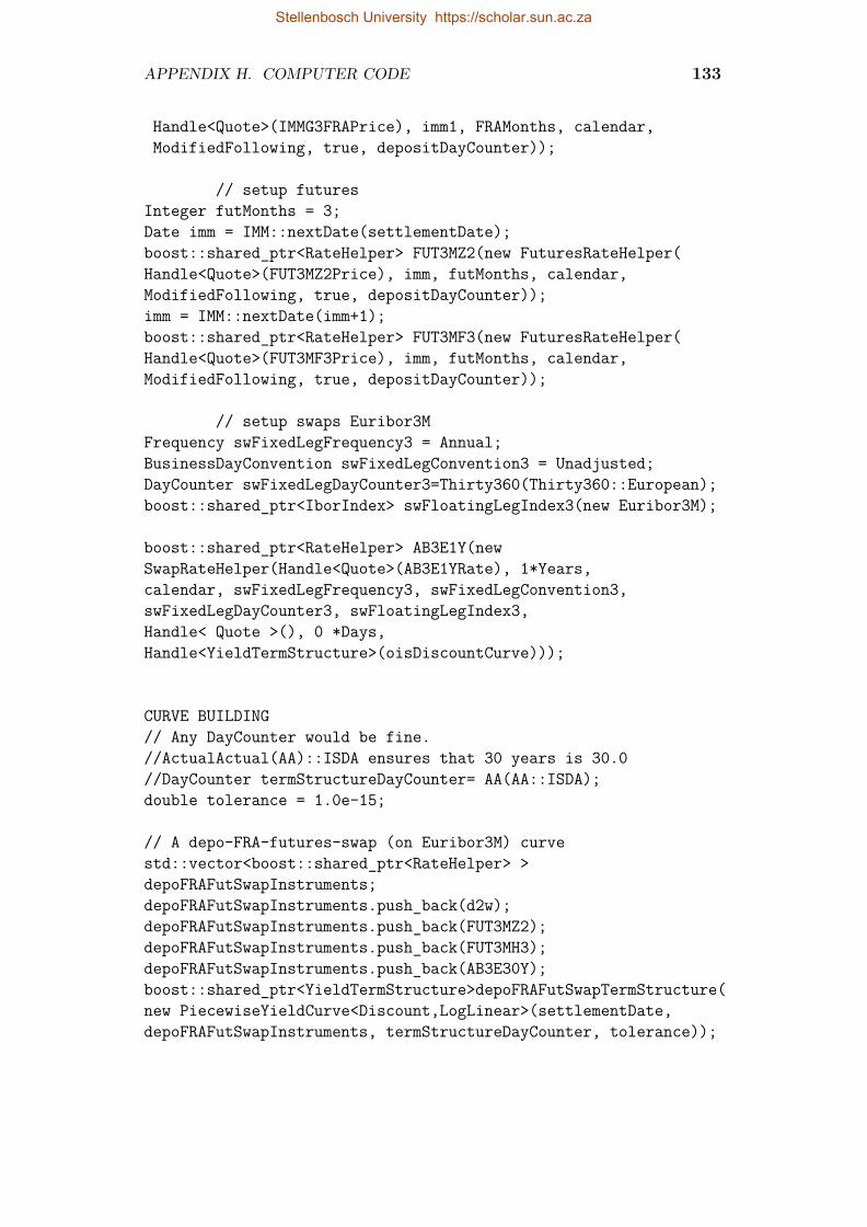
APPENDIX H. COMPUTER CODE 133
Handle<Quote>(IMMG3FRAPrice), imm1, FRAMonths, calendar,ModifiedFollowing, true, depositDayCounter));
// setup futuresInteger futMonths = 3;Date imm = IMM::nextDate(settlementDate);boost::shared_ptr<RateHelper> FUT3MZ2(new FuturesRateHelper(Handle<Quote>(FUT3MZ2Price), imm, futMonths, calendar,ModifiedFollowing, true, depositDayCounter));imm = IMM::nextDate(imm+1);boost::shared_ptr<RateHelper> FUT3MF3(new FuturesRateHelper(Handle<Quote>(FUT3MF3Price), imm, futMonths, calendar,ModifiedFollowing, true, depositDayCounter));
// setup swaps Euribor3MFrequency swFixedLegFrequency3 = Annual;BusinessDayConvention swFixedLegConvention3 = Unadjusted;DayCounter swFixedLegDayCounter3=Thirty360(Thirty360::European);boost::shared_ptr<IborIndex> swFloatingLegIndex3(new Euribor3M);
boost::shared_ptr<RateHelper> AB3E1Y(newSwapRateHelper(Handle<Quote>(AB3E1YRate), 1*Years,calendar, swFixedLegFrequency3, swFixedLegConvention3,swFixedLegDayCounter3, swFloatingLegIndex3,Handle< Quote >(), 0 *Days,Handle<YieldTermStructure>(oisDiscountCurve)));
CURVE BUILDING// Any DayCounter would be fine.//ActualActual(AA)::ISDA ensures that 30 years is 30.0//DayCounter termStructureDayCounter= AA(AA::ISDA);double tolerance = 1.0e-15;
// A depo-FRA-futures-swap (on Euribor3M) curvestd::vector<boost::shared_ptr<RateHelper> >depoFRAFutSwapInstruments;depoFRAFutSwapInstruments.push_back(d2w);depoFRAFutSwapInstruments.push_back(FUT3MZ2);depoFRAFutSwapInstruments.push_back(FUT3MH3);depoFRAFutSwapInstruments.push_back(AB3E30Y);boost::shared_ptr<YieldTermStructure>depoFRAFutSwapTermStructure(new PiecewiseYieldCurve<Discount,LogLinear>(settlementDate,depoFRAFutSwapInstruments, termStructureDayCounter, tolerance));
Stellenbosch University https://scholar.sun.ac.za

List of References
Ametrano, F. and Bianchetti, M. (2009). Bootstrapping the Illiquidity: MultipleYield Curves Construction for Market Coherent Forward Rates Estimation. In“Modeling Interest Rates: Advances for Derivatives Pricing”, edited by F. Mer-curio, Risk Books.
Ametrano, F.M. (2011). Rates curves for forward Euribor estimation and CSA-discounting. QuantLib Forum, London, 18 Jan. 2011.
Ametrano, F.M. and Bianchetti, M. (2013). Everything You Always Wanted toKnow About Multiple Interest Rate Curve Bootstrapping But Were Afraid toAsk. Available at: http: // ssrn. com/ abstract= 2219548 .
Andersen, L. (2007). Discount curve construction with tension splines. Review ofDerivatives Research, vol. 10, no. 3, pp. 227–267.
Andersen, L. and Andreasen, J. (2000). Jump-Diffusion Processes: Volatility SmileFitting and Numerical Methods for Option Pricing. Review of Derivatives Re-search, vol. 4, no. 3, pp. 231–262.
Bates, D.S. (1996). Jumps and Stochastic Volatility: Exchange Rate ProcessesImplicit in Deutsche Mark Options. Review of financial studies, vol. 9, no. 1, pp.69–107.
Benaim, S., Friz, P. and Lee, R. (2008). On Black-Scholes Implied Volatility atExtreme Strikes. Frontiers in Quantitative Finance: Volatility and Credit RiskModeling, pp. 19–45.
Berestycki, H., Busca, J. and Florent, I. (2002). Asymptotics and calibration of localvolatility models. Quantitative finance, vol. 2, no. 1, pp. 61–69.
Berestycki, H., Busca, J. and Florent, I. (2004). Computing the implied volatility instochastic volatility models. Communications on Pure and Applied Mathematics,vol. 57, no. 10, pp. 1352–1373.
Bianchetti, M. (2008). Two Curves, One Price: Pricing & Hedging Interest RateDerivatives Decoupling Forwarding and Discounting Yield Curves. Risk Magazine.
Bianchetti, M. and Carlicchi, M. (2011). Interest Rates After The Credit Crunch:Multiple-Curve Vanilla Derivatives and SABR. The Capco Journal of FinancialTransformation, Applied Finance n. 32, September.
134
Stellenbosch University https://scholar.sun.ac.za

LIST OF REFERENCES 135
Black, F., Derman, E. and Toy, W. (1990). A One-Factor Model of Interest Ratesand its Application to Treasury Bond Options. Financial analysts journal, pp.33–39.
Black, F. and Karasinski, P. (1991). Bond and Option Pricing When Short Ratesare Lognormal. Financial Analysts Journal, pp. 52–59.
Bulirsch, R. and Stoer, J. (2002). Introduction to Numerical Analysis. SpringerHeidelberg.
Carr, P., Geman, H., Madan 5, D.B. and Yor, M. (2004). From Local Volatility toLocal Lévy Models. Quantitative Finance, vol. 4, no. 5, pp. 581–588.
Carr, P. and Wu, L. (2007). Stochastic Skew in Currency Options. Journal ofFinancial Economics, vol. 86, no. 1, pp. 213–247.
Castagna, A. (2012). Pricing of Collateralized Derivatives Contracts When Morethan One Currency are Involved: Liquidity and Funding Value Adjustments.Available at: http: // ssrn. com/ abstract= 2073300 .
Chevalier, E. (2005). Critical Price near Maturity for an American Option ona Dividend-Paying Stock in a Local Volatility Model. Mathematical Finance,vol. 15, no. 3, pp. 439–463.
Chibane, M., Selvaraj, J. and Sheldon, G. (2009). Building Curves on a Good Basis.Available at: http: // ssrn. com/ abstract= 1394267 .
Derman, E. and Kani, I. (1998). Stochastic Implied Trees: Arbitrage Pricing withStochastic Term and Strike Structure of Volatility. International Journal of The-oretical and Applied Finance, vol. 1, no. 01, pp. 61–110.
Derman, E., Kani, I. and Chriss, N. (1996). Implied Trinomial Trees of the VolatilitySmile. The Journal of Derivatives, vol. 3, no. 4, pp. 7–22.
Doust, P. (2012). No-Arbitrage SABR. Journal of Computational Finance, vol. 15,no. 3, p. 3.
Duffy, D.J. and Germani, A. (2013). C# for Financial Markets. John Wiley & Sons.
Dupire, B. (1994). Pricing with a smile. Risk Magazine, pp. 18–20.
Dupire, B. (1997). Pricing and Hedging with Smiles. Mathematics of derivativesecurities, edited by M.A.H. Dempster and S.R. Pliska, Cambridge UniversityPress, Cambridge, 103-111.
Ekstrand, C. (2011). Financial Derivatives Modeling. Springer.
Errais, E., Mauri, G. and Mercurio, F. (2004). Capturing the Skew in Interest RateDerivatives: A Shifted Lognormal LIBOR Model with Uncertain Parameters.Tech. Rep., Internal Report, Stanford University and Banca IMI.
Stellenbosch University https://scholar.sun.ac.za

LIST OF REFERENCES 136
Fujii, M., Shimada, Y. and Takahashi, A. (2010). Collateral Posting and Choiceof Collateral Currency-Implications for Derivative Pricing and Risk Management.Available at: http: // ssrn. com/ abstract= 1601866 .
Fujii, M. and Takahashi, A. (2011). Choice of Collateral Currency. Risk Magazine,vol. 24, no. 1, pp. 120–125.
Gatheral, J. (2006). The Volatility Surface: A Practitioner’s Guide, vol. 357. JohnWiley & Sons.
Gatheral, J., Hsu, E.P., Laurence, P., Ouyang, C. and Wang, T.-H. (2012). Asymp-totics of Implied Volatility in Local Volatility Models. Mathematical Finance,vol. 22, no. 4, pp. 591–620.
Gibbs, M. and Goyder, R. (2012). The Past, Present, Future of Curves. FINCAD.
Hagan, P., Lesniewski, A. and Woodward, D. (2005). Probability Distribution inthe SABR Model of Stochastic Volatility. preprint.
Hagan, P.S., Kumar, D., Lesniewski, A. and Woodward, D. (2014). Arbitrage-FreeSABR. Wilmott, vol. 2014, no. 69, pp. 60–75.
Hagan, P.S., Kumar, D., Lesniewski, A.S. and Woodward, D.E. (2002). ManagingSmile Risk. Wilmott Magazine, July, pp. 84–108.
Hagan, P.S. and West, G. (2006). Interpolation Methods for Curve Construction.Applied Mathematical Finance, vol. 13, no. 2, pp. 89–129.
Hagan, P.S. and West, G. (2008). Methods for Constructing a Yield Curve. WilmottMagazine, May, pp. 70–81.
Hagan, P.S. and Woodward, D.E. (1999). Equivalent Black Volatilities. AppliedMathematical Finance, vol. 6, no. 3, pp. 147–157.
Harrison, J.M. and Kreps, D.M. (1979). Martingales and Arbitrage in MultiperiodSecurities Markets. Journal of Economic theory, vol. 20, no. 3, pp. 381–408.
Harrison, J.M. and Pliska, S.R. (1981). Martingales and Stochastic Integrals inthe Theory of Continuous Trading. Stochastic processes and their applications,vol. 11, no. 3, pp. 215–260.
Harrison, J.M. and Pliska, S.R. (1983). A Stochastic Calculus Model of ContinuousCrading: Complete Markets. Stochastic processes and their applications, vol. 15,no. 3, pp. 313–316.
Henrard, M. (2013). Multi-Curve Framework with Collateral. OpenGamma.
Henry-Labordere, P. (2005). A General Asymptotic Implied Volatility for StochasticVolatility Models. Available at: http: // ssrn. com/ abstract= 698601 .
Henry-Labordere, P. (2006). Unifying the BGM and SABR Models: A short Ridein Hyperbolic Geometry. Available at: http: // ssrn. com/ abstract= 877762 .
Stellenbosch University https://scholar.sun.ac.za

LIST OF REFERENCES 137
Heston, S.L. (1993). A Closed-Form Solution for Options with Stochastic Volatilitywith Applications to Bond and Currency Options. Review of financial studies,vol. 6, no. 2, pp. 327–343.
Ho, T.S. and Lee, S.B. (1986). Term Structure Movements and Pricing Interest RateContingent Claims. The Journal of Finance, vol. 41, no. 5, pp. 1011–1029.
Hobson, D.G. and Rogers, L.C. (1998). Complete Models with Stochastic Solatility.Mathematical Finance, vol. 8, no. 1, pp. 27–48.
Holmes, M.H. (2012). Introduction to Perturbation Methods, vol. 20. Springer.
Hull, J. (2009). Options, Futures and Other Derivatives. Pearson education.
Hull, J. and White, A. (1987). The Pricing of Options on Assets with StochasticVolatilities. The journal of finance, vol. 42, no. 2, pp. 281–300.
Hull, J. andWhite, A. (1993). One-Factor Interest-Rate Models and the Valuation ofInterest-Rate Derivative Securities. Journal of financial and quantitative analysis,vol. 28, no. 02, pp. 235–254.
Kalotay, A.J., Williams, G.O. and Fabozzi, F.J. (1993). A Model for Valuing Bondsand Embedded Options. Financial Analysts Journal, pp. 35–46.
Kienitz, J. (2013). Transforming Volatility-Multi Curve Cap and SwaptionVolatilities. Available at: http: // ssrn. com/ abstract= 2204702 .
Lee, R.W. (2004). The Moment Formula for Implied Volatility at Extreme Strikes.Mathematical Finance, vol. 14, no. 3, pp. 469–480.
Masaaki, F. and Akihiko, T. (2011). Clean Valuation Framework for the USD Silo-An Implication for the Forthcoming Standard Credit Support Annex (SCSA).Available at: http: // ssrn. com/ abstract= 1969686 .
Masaaki, F., Yasufumi, S. and Akihiko, T. (2010a). Modeling of Interest Rate TermStructures Under Collateralization and its Implications. Available at: http:// ssrn. com/ abstract= 1681910 .
Masaaki, F., Yasufumi, S. and Akihiko, T. (2010b). On the Term Structure ofInterest Rates with Basis Spread. Available at: http: // ssrn. com/ abstract=1556487 .
Mbongo, J. (2014). Yield Curves Codes. https://sites.google.com/a/aims.ac.za/jeffrey-mbongo/msc-code.
Mercurio, F. (2010). LIBOR Market Models with Stochastic Basis. Risk Magazine,vol. 23, no. 12, pp. 84–89.
Mercurio, F. and Pallavicini, A. (2006). Smiling at Convexity: Bridging SwaptionSkews and CMS Adjustments. Available at: http: // ssrn. com/ abstract=892287 .
Stellenbosch University https://scholar.sun.ac.za

LIST OF REFERENCES 138
Merton, R.C. (1971). Theory of rational option pricing.
Morini, M. and Mercurio, F. (2007). No-Arbitrage Dynamics for a Tractable SABRTerm Structure Libor Model. Bloomberg Portfolio Research Paper.
Oblój, J. (2008). FINE-TUNE YOUR SMILE: CORRECTION to HAGAN ET AL.Wilmott Magazine, 35, pp. 102–104.
Oleksandr, D., Yining, G. and Cem, Sinan, O. (2014). Interest rates after thecredit crunch crisis: SINGLE versus MULTIPLE curve approach. Master’s thesis,Barcelona GSE Master Project, http://www.slideshare.net/barcelonagse/interest-ratescreditpaper.
Piterbarg, V. (2003). A Stochastic Volatility Forward Libor Model with a TermStructure of Volatility Smiles. Available at: http: // ssrn. com/ abstract=472061 .
Piterbarg, V. (2012). Cooking with collateral. Risk Magazine, vol. 8.
Rebonato, R. and Rebonato, R. (1998). Interest-Rate Option Models, vol. 2. WileyNew York.
Rogers, L. and Veraart, L.A. (2008). A Stochastic Volatility Alternative to SABR.Journal of Applied Probability, pp. 1071–1085.
Ron, U. (2000). A Practical Guide to Swap Curve Construction. Bank of Canada.
Roper, M. (2010). Arbitrage free Implied Volatility Surfaces. preprint.
Shreve, S.E. (2004). Stochastic Calculus for Finance II: Continuous-Time Models,vol. 11. Springer.
Stein, E.M. and Stein, J.C. (1991). Stock Price Distributions with StochasticVolatility: an Analytic Approach. Review of financial Studies, vol. 4, no. 4,pp. 727–752.
QuantLib (Open Source). http://quantlib.org/index.shtml.
West, G. (2005). Calibration of the SABR model in Illiquid Markets. AppliedMathematical Finance, vol. 12, no. 4, pp. 371–385.
Wiggins, J.B. (1987). Option values under stochastic volatility: Theory and empir-ical estimates. Journal of financial economics, vol. 19, no. 2, pp. 351–372.
Stellenbosch University https://scholar.sun.ac.za