Interpretable classifiers using rules and Bayesian analysis: Building a better stroke

prediction model

Benjamin Letham Cynthia Rudin MIT MIT

Tyler H. McCormick David Madigan

University of Washington Columbia University

Technical Report no. 609 Department of Statistics

University of Washington August 2013

Interpretable classifiers using rules and Bayesian analysis:

Building a better stroke prediction model

Benjamin Letham, Operations Research Center, Massachusetts Institute of Tech-nology. bletham@mit.edu

Cynthia Rudin, Computer Science and Artificial Intelligence Laboratory, MassachusettsInstitute of Technology. rudin@mit.edu

Tyler H. McCormick, Department of Statistics, Department of Sociology, Center forStatistics and the Social Sciences, University of Washington. tylermc@u.washington.edu

David Madigan, Department of Statistics, Columbia University. madigan@stat.columbia.edu

Abstract

We aim to produce predictive models that are not only accurate, but are alsointerpretable to human experts. Our models are decision lists, which consist of aseries of if...then... statements (for example, if high blood pressure, then stroke) thatdiscretize a high-dimensional, multivariate feature space into a series of simple, readilyinterpretable decision statements. We introduce a generative model called BayesianRule Lists that yields a posterior distribution over possible decision lists. It employs anovel prior structure to encourage sparsity. Our experiments show that Bayesian RuleLists has predictive accuracy on par with the current top algorithms for prediction inmachine learning. Our method is motivated by recent developments in personalizedmedicine, and can be used to produce highly accurate and interpretable medical scoringsystems. We demonstrate this by producing an alternative to the CHADS2 score,actively used in clinical practice for estimating the risk of stroke in patients that haveatrial fibrillation. Our model is as interpretable as CHADS2, but more accurate.

1 Introduction

Our goal is to build predictive models that are highly accurate, yet are highly interpretable.These predictive models will be in the form of sparse decision lists, which consist of a seriesof if... then... statements where the if statements define a partition of a set of features andthe then statements correspond to the predicted outcome of interest. Because of this form,a decision list model naturally provides a reason for each prediction that it makes. Figure 1presents an example decision list that we created using the Titanic dataset available in R.This dataset provides details about each passenger on the Titanic, including whether thepassenger was an adult or child, male or female, and their class (1st, 2nd, 3rd, or crew).The goal is to predict whether the passenger survived based on his or her features. The listprovides an explanation for each prediction that is made. For example, we predict that apassenger is less likely to survive than not because he or she was in the 3rd class. The list in

1

if male and adult then survival probability 21% (19% - 23%)else if 3rd class then survival probability 44% (38% - 51%)else if 1st class then survival probability 96% (92% - 99%)else survival probability 88% (82% - 94%)

Figure 1: Decision list for Titanic. In parentheses is the 95% credible interval for the survivalprobability.

Fig. 1 is one accurate and interpretable decision list for predicting survival on the Titanic,possibly one of many such lists. Our goal is to learn these lists from data.

Our model, called Bayesian Rule Lists (BRL), produces a posterior distribution overpermutations of if... then... rules, starting from a large, pre-mined set of possible rules.The decision lists with high posterior probability tend to be both accurate and interpretable,where the interpretability comes from a hierarchical prior over permutations of rules. Theprior favors concise decision lists that have a small number of total rules, where the ruleshave few terms in the left-hand side.

BRL provides a new type of balance between accuracy, interpretability and computation.Consider the challenge of constructing a predictive model that discretizes the input space inthe same way as decision trees [Breiman et al., 1984, Quinlan, 1993], decision lists [Rivest,1987] or associative classifiers [Liu et al., 1998]. Greedy construction methods like classifica-tion and regression trees (CART) or C5.0 are not particularly computationally demanding,but in practice the greediness heavily affects the quality of the solution, both in terms ofaccuracy and interpretability. At the same time, optimizing a decision tree over the fullspace of all possible splits is not a tractable problem. BRL strikes a balance between theseextremes, in that its solutions are not constructed in a greedy way, yet it can solve problemsat the scale required to have an impact in real problems in science or society, includingmodern healthcare.

A major source of BRL’s practical feasibility is the fact that it uses pre-mined rules,which reduces the model space to that of permutations of rules as opposed to all possiblesets of splits. The complexity of the problem then depends on the number of pre-minedrules rather than on the full space of feature combinations. As long as the pre-mined setof rules is sufficiently expressive, an accurate decision list can be found, and in fact thesmaller model space might improve generalization [through the lens of statistical learningtheory, Vapnik, 1995]. An additional advantage to using pre-mined rules is that each ruleis independently both interpretable and informative about the data.

BRL’s prior structure encourages decision lists that are sparse. Sparse decision lists servenot only the purpose of producing a more interpretable model, but also reduce computation,as most of the sampling iterations take place within a small set of permutations correspond-ing to the sparse decision lists. In practice, BRL is able to compute predictive models withaccuracy comparable to state-of-the-art machine learning methods, yet maintain the samelevel of interpretability as medical scoring systems.

The motivation for our work lies in developing interpretable patient-level predictivemodels using massive observational medical data. To this end, we use BRL to construct analternative to the CHADS2 score of Gage et al. [2001]. CHADS2 is widely-used in medical

2

practice to predict stroke in patients with atrial fibrillation. A patient’s CHADS2 score iscomputed by assigning one “point” each for the presence of congestive heart failure (C),hypertension (H), age 75 years or older (A), and diabetes mellitus (D), and by assigning2 points for history of stroke, transient ischemic attack, or thromoembolism (S2). TheCHADS2 score considers only 5 factors, whereas the updated CHA2DS2-VASc score [Lipet al., 2010b] includes three additional risk factors: vascular disease (V), age 65 to 74 yearsold (A), and female gender (Sc). Higher scores correspond to increased risk. In the studydefining the CHADS2 score [Gage et al., 2001], the scores was calibrated with stroke risksusing a database of 1,733 Medicare beneficiaries followed for, on average, about a year.

Our alternative to the CHADS2 was constructed using 12,586 patients and 4,148 factors.Because we are using statistical learning, we are able to consider significantly more features;this constitutes over 5000 times the amount of data used for the original CHADS2 study. Inour experiments we compared the stroke prediction performance of BRL to CHADS2 andCHA2DS2-VASc, as well as to a collection of state-of-the-art machine learning algorithms:C5.0 [Quinlan, 1993], CART [Breiman et al., 1984], `1-regularized logistic regression, sup-port vector machines [Vapnik, 1995], random forests [Breiman, 2001], and Bayesian CART[Dension et al., 1998, Chipman et al., 1998]. The balance of accuracy and interpretabilityobtained by BRL is not easy to obtain through other means: None of the machine learn-ing methods we tried could obtain both the same level of accuracy and the same level ofinterpretability.

2 Bayesian Rule Lists

The setting for BRL is multi-class classification, where the set of possible labels is 1, . . . , L.In the case of predicting stroke risk, there are two labels: stroke or no stroke. The trainingdata are pairs {(xi, yi)}ni=1, where xi ∈ Rd are the features of observation i, and yi are thelabels, yi ∈ {1, . . . , L}. We let x = (x1, . . . , xn) and y = (y1, . . . , yn).

In Sections 2.1 and 2.2 we provide the association rule concepts and notation upon whichthe method is built. Section 2.3 introduces BRL by outlining the generative model. Sections2.4 and 2.5 provide detailed descriptions of the prior and likelihood, and then Sections 2.6and 2.7 describe sampling and posterior predictive distributions.

2.1 Bayesian association rules and Bayesian decision lists

An association rule a → b is an implication with an antecedent a and a consequent b. Forthe purposes of classification, the antecedent is an assertion about the feature vector xithat is either true or false, for example, “xi,1 = 1 and xi,2 = 0.” This antecedent containstwo conditions, which we call the cardinality of the antecedent. The consequent b wouldtypically be a predicted label y. A Bayesian association rule has a multinomial distributionover labels as its consequent rather than a single label:

a→ y ∼ Multinomial(θ).

The multinomial probability is then given a prior, leading to a prior consequent distribution:

θ|α ∼ Dirichlet(α)

Given observations (x,y) classified by this rule, we let N·,l be the number of observationswith label yi = l, and N = (N·,1, . . . , N·,L). We then obtain a posterior consequent distri-

3

bution:θ|x,y, α ∼ Dirichlet(α+N).

The core of a Bayesian decision list is an ordered antecedent list d = (a1, . . . , am). LetNj,l be the number of observations xi that satisfy aj but not any of a1, . . . , aj−1, and thathave label yi = l. This is the number of observations to be classified by antecedent aj thathave label l. Let N0,l be the number of observations that do not satisfy any of a1, . . . , am,and that have label l. Let Nj = (Nj,1, . . . , Nj,L) and N = (N0, . . . ,Nm).

A Bayesian decision list D = (d, α,N) is an ordered list of antecedents together withtheir posterior consequent distributions, which are obtained by excluding data that havesatisfied an earlier antecedent in the list:

if a1 then y ∼ Multinomial(θ1), θ1 ∼ Dirichlet(α+ N1)else if a2 then y ∼ Multinomial(θ2), θ2 ∼ Dirichlet(α+ N2)...else if am then y ∼ Multinomial(θm), θm ∼ Dirichlet(α+ Nm)else y ∼ Multinomial(θ0), θ0 ∼ Dirichlet(α+ N0).

Any observations that do not satisfy any of the antecedents in d are classified using theparameter θ0, which we call the default rule parameter.

2.2 Antecedent mining

We are interested in forming Bayesian decision lists whose antecedents are a subset of apre-selected collection of antecedents. For data with binary or categorical features thiscan be done using frequent itemset mining, where itemsets are used as antecedents. Inour experiments, the features were binary and we used the FP-Growth algorithm [Borgelt,2005] for antecedent mining, which finds all itemsets that satisfy constraints on minimumsupport and maximum cardinality. This means each antecedent applies to a sufficientlylarge amount of data and does not have too many conditions. The particular choice of theitemset mining algorithm is unimportant as the output is an exhaustive list of all itemsetssatisfying the constraints. Because the goal is to obtain decision lists with few rules and fewconditions per rule, we need not include any itemsets that apply only to a small numberof observations or have a large number of conditions. Thus frequent itemset mining allowsus to significantly reduce the size of the feature space, compared to considering all possiblecombinations of features.

The frequent itemset mining that we do in our experiments produces only antecedentswith sets of features, such as “diabetes and heart disease.” Other techniques could be usedfor mining antecedents with negation, such as “not diabetes” [Wu et al., 2004]. For datawith continuous features, a variety of procedures exist for antecedent mining [Fayyad andIrani, 1993, Dougherty et al., 1995, Srikant and Agrawal, 1996], or one can create categoricalfeatures using interpretable thresholds (e.g, ages 40-49, 50-59, etc.) or interpretable quantiles(e.g., quartiles).

We let A represent the complete, pre-mined collection of antecedents, and suppose thatA contains R antecedents with up to C conditions in each antecedent.

4

2.3 Generative model

We now sketch the generative model for the labels y from the observations x and antecedentsA.

– Sample a decision list length m ∼ p(m|λ).

– Sample the default rule parameter θ0 ∼ Dirichlet(α).

– For decision list rule j = 1, . . . ,m:

Sample the cardinality of antecedent aj in d as cj ∼ p(cj |η).

Sample aj of cardinality cj from p(aj |a1, . . . , aj−1, cj ,A).

Sample rule consequent parameter θj ∼ Dirichlet(α).

– For observation i = 1, . . . , n:

Find the antecedent aj in d that is the first that applies to xi.

If no antecedents in d apply, set j = 0.

Sample yi ∼ Multinomial(θj).

Our goal is to sample from the posterior distribution over antecedent lists:

p(d|x,y,A, α, λ, η) ∝ p(y|x, d, α)p(d|A, λ, η).

Given d, we can compute the posterior consequent distributions required to construct aBayesian decision list as in Section 2.1. There are three prior hyperparameters that mustbe specified by the user: α, λ, and η. We will see in Sections 2.4 and 2.5 that thesehyperparameters have natural interpretations that suggest the values to which they shouldbe set.

2.4 The hierarchical prior for antecedent lists

Suppose the list of antecedents d has length m and antecedent cardinalities c1, . . . , cm. Theprior probability of d is defined hierarchically as

p(d|A, λ, η) = p(m|A, λ)

m∏j=1

p(cj |c1, . . . , cj−1,A, η)p(aj |a1, . . . , aj−1, cj ,A).

We take the distributions for list length m and antecedent cardinality cj to be Poisson withparameters λ and η respectively, with proper truncation to account for the finite numberof antecedents in A. Specifically, the distribution of m is Poisson truncated at the totalnumber of pre-selected antecedents:

p(m|A, λ) =(λm/m!)∑Rj=0(λj/j!)

, m = 0, . . . , R.

This truncated Poisson is a proper prior, and is natural choice because of its simple parame-terization. Specifically, this prior has the desirable property that when R is large compared

5

to the desired size of the decision list, as will generally be the case when seeking an in-terpretable decision list, the prior expected decision list length E[m|A, λ] is approximatelyequal to λ. The prior hyperparameter λ can then naturally be set to the prior belief of thelist length required to model the data. A Poisson distribution is used in a similar way inthe hierarchical prior of Wu et al. [2007].

The distribution of cj must be truncated at zero and at the maximum antecedent cardi-nality C. Additionally, any cardinalities that have been exhausted by point j in the decisionlist sampling must be excluded. Let Rj(c1, . . . , cj ,A) be the set of antecedent cardinalitiesthat are available after drawing antecedent j. For example, if A contains antecedents of size1, 2, and 4, then we begin with R0(A) = {1, 2, 4}. If A contains only 2 rules of size 4 andc1 = c2 = 4, then R2(c1, c2,A) = {1, 2} as antecedents of size 4 have been exhausted. Wenow take p(cj |c1, . . . , cj−1,A, η) as Poisson truncated to remove values for which there areno rules available with that cardinality:

p(cj |c1, . . . , cj−1,A, η) =(ηcj/cj !)∑

k∈Rj−1(c1,...,cj−1,A)(ηk/k!)

,

cj ∈ Rj−1(c1, . . . , cj−1,A).

If the number of rules of different sizes is large compared to λ, and η is small compared toC, the prior expected average antecedent cardinality is close to η. Thus η can naturally beset to the prior belief of the antecedent cardinality required to model the data.

Once the antecedent cardinality cj has been selected, the antecedent aj must be sampledfrom all available antecedents in A of size cj . If there were a preference towards specificantecedents, e.g. antecedents that are particularly interpretable, this preference could beexpressed in p(aj |a1, . . . , aj−1, cj ,A). Here, we use a uniform distribution over antecedentsin A of size cj , excluding those in {a1, . . . , aj−1}. Let Qk(A, a1, . . . , aj−1) = {a ∈ A \{a1, . . . , aj−1} : |a| = k}. Then,

p(aj |a1, . . . , aj−1, cj ,A) =1

|Qcj (A, a1, . . . , aj−1)|,

aj ∈ Qcj (A, a1, . . . , aj−1).

It is straightforward to sample an ordered antecedent list d from the prior by following thegenerative model, using the provided distributions.

2.5 The likelihood function

The likelihood function follows directly from the generative model. Let θ = (θ0, θ1, . . . , θm)be the consequent parameters corresponding to each antecedent in d, together with thedefault rule parameter θ0. Then,

p(y|x, d, θ) =∏

j=0,...,m,∑lNj,l>0

Multinomial(Nj |θj),

withθj ∼ Dirichlet(α).

6

We can marginalize over θj in each Multinomial distribution in the above product, obtaining,through the standard derivation of the Dirichlet-Multinomial distribution,

p(y|x, d, α) =∏

j=0,...,m,∑lNj,l>0

Γ(∑Ll=1 αl)

Γ(∑Ll=1Nj,l + αl)

×L∏l=1

Γ(Nj,l + αl)

Γ(αl)

∝∏

j=0,...,m,∑lNj,l>0

∏Ll=1 Γ(Nj,l + αl)

Γ(∑Ll=1Nj,l + αl)

.

The prior hyperparameter α has the usual Bayesian interpretation of pseudocounts. Inour experiments, we set αl = 1 for all l, producing a uniform prior.

2.6 Markov chain Monte Carlo sampling

We do Metropolis-Hastings sampling of d, generating the proposed d∗ from the current dt

using one of three options: 1) Move an antecedent in dt to a different position in the list. 2)Add an antecedent from A that is not currently in dt into the list. 3) Remove an antecedentfrom dt. Which antecedents to adjust and their new positions are chosen uniformly atrandom at each step. The option to move, add, or remove is also chosen uniformly. Theprobabilities for the proposal distribution Q(d∗|dt) depend on the size of the antecedentlist, the number of pre-mined antecedents, and whether the proposal is a move, addition,or removal. For the uniform distribution that we used, the proposal probabilities for a d∗

produced by one of the three proposal types is:

Q(d∗|dt,A) =

1

(|dt|)(|dt|−1) if move proposal,1

(|A|−|dt|)(|dt|+1) if add proposal,1|dt| if remove proposal.

To explain these probabilities, if there is a move proposal, we consider the number of possibleantecedents to move and the number of possible positions to move to; if there is an addproposal, we consider the number of possible antecedents to add to the list and the numberof positions to place a new antecedent; for remove proposals we consider the number ofpossible antecedents to remove. This sampling algorithm is related to those used for BayesianDecision Tree models [Chipman et al., 2002, 1998, Wu et al., 2007] and to methods forexploring tree spaces [Madigan et al., 2011].

For every MCMC run, we ran 3 chains, each initialized independently from a randomsample from the prior. We discarded the first half of simulations as burn-in, and thenassessed chain convergence using the Gelman-Rubin convergence diagnostic applied to thelog posterior density [Gelman and Rubin, 1992]. We considered chains to have convergedwhen the diagnostic R < 1.05.

2.7 The posterior predictive distribution and point estimates

Given the posterior p(d|x,y,A, α, λ, η), we consider estimating the label y of a new observa-tion x using either a point estimate (a single interpretable model) or the posterior predictive

7

distribution. Given a point estimate of the antecedent list d, we have that

p(y = l|x, d,x,y, α) =

∫θ

θlp(θ|x, d,x,y, α)dθ

= E[θl|x, d,x,y, α].

Let j(d, x) be the index of the first antecedent in d that applies to x. The posterior conse-quent distribution is

θ|x, d,x,y, α ∼ Dirichlet(α+ Nj(d,x)

). (1)

Thus,

p(y = l|x, d,x,y, α) =αl +Nj(d,x),l∑L

k=1

(αk +Nj(d,x),k

) .Additionally, (1) allows for the estimation of 95% credible intervals using the Dirichletdistribution function..

The posterior mean is often a good choice for a point estimate, however since the posterioris a distribution over antecedent lists there is not a clear notion of its mean. We thus look foran antecedent list whose statistics are similar to the posterior mean statistics. Specifically,we are interested in finding a point estimate d whose length m and whose average antecedentcardinality c = 1

m

∑mj=1 cj are close to the posterior mean list length and average cardinality.

Let m be the posterior mean decision list length and ¯c the posterior mean average antecedentcardinality, as estimated from the MCMC samples. Then, we choose our point estimate das the list with the highest posterior probability among all samples with m ∈ {bmc , dme}and c ∈ [b¯cc , d¯ce]. We call this point estimate BRL-point.

Alternatively, we can use the entire posterior p(d|x,y,A, α, λ, η) to estimate y. Theposterior predictive distribution for y is

p(y = l|x,x,y,A, α, λ, η) =∑d∈D

p(y = l|x, d,x,y,A, α)p(d|x,y,A, α, λ, η)

=∑d∈D

αl +Nj(d,x),l∑Lk=1

(αk +Nj(d,x),k

)p(d|x,y,A, α, λ, η)

where D is the set of all ordered subsets of A. The posterior samples obtained by MCMCsimulation can be used to approximate this sum. We call the classifier that uses the fullcollection of posterior samples BRL-post. Using the entire posterior distribution to makea prediction means the classifier is no longer interpretable. One could, however, use theposterior predictive distribution to classify, and then provide several point estimates fromthe posterior to the user as example explanations for the prediction.

3 Simulation studies

We use simulation studies and a deterministic dataset to show that when data are generatedby a decision list model, the BRL method is able to recover the true decision list.

3.1 Simulated data sets

Given observations with arbitrary features, and a collection of rules on those features, we canconstruct a binary matrix where the rows represent observations and the columns represent

8

0 1 2 3 4 5Number of observations

0

1

2

3

4

5Po

ster

ior

mea

ndi

stan

ceto

the

true

deci

sion

list

(a)

×1030 1 2 3 4 5

Distance to the true decision list

0.0

0.2

0.4

0.6

0.8

1.0

Tota

lpos

teri

orpr

obab

ility

(b)

n = 100

n = 5000

Figure 2: (a) Average Levenshtein distance from posterior samples to the true decision list,for differing numbers of observations. The black solid line indicates the median value acrossthe 100 simulated datasets of each size, and the gray dashed lines indicate the first and thirdquartiles. (b) The proportion of posterior samples with the specified distance to the truedecision list, for a randomly selected simulation with n = 100 observations and a randomlyselected simulation with n = 5000.

rules, and the entry is 1 if the rule applies to that observation and 0 otherwise. We needonly simulate this binary matrix to represent the observations without losing generality. Forour simulations, we generated independent binary rule sets with 100 rules by setting eachfeature value to 1 independently with probability 1/2.

We generated a random decision list of size 5 by selecting 5 rules at random, and addingthe default rule. Each rule in the decision list was assigned a consequent distribution overlabels using a random draw from the Beta(1/2, 1/2) distribution, which ensures that therules are informative about labels. Labels were then assigned to each observation using thedecision list: For each observation, the label was taken as a draw from the label distributioncorresponding to the first rule that applied to that observation.

For each number of observations N ∈ {100, 250, 500, 1000, 2500, 5000}, we generated 100independent data sets (x,y), for a total of 600 simulated datasets. We did MCMC samplingwith three chains as described in Section 2 for each dataset. For all datasets, 20,000 sampleswere sufficient for the chains to converge.

To appropriately visualize the posterior distribution, we binned the posterior antecedentlists according to their distance from the true antecedent list, using the Levenshtein stringedit distance [Levenshtein, 1966] to measure the distance between two antecedent lists. Thismetric measures the minimum number of antecedent substitutions, additions, or removalsto transform one decision list into the other. The results of the simulations are given inFig. 2. Figure 2(a) shows that as the number of observations increases, the posterior massconcentrates on the true decision list. Figure 2(b) illustrates this concentration with twochoices of the distribution of posterior distances to the true decision list, for n small and forn large.

3.2 A deterministic problem

We fit BRL to the Tic-Tac-Toe Endgame dataset from the UCI Machine Learning Repository[Bache and Lichman, 2013] of benchmark datasets. The Tic-Tac-Toe Endgame datasetprovides all possible end board configurations for the game Tic-Tac-Toe, with the task of

9

Table 1: Mean classification accuracy in the top row, with standard deviation in the secondrow, for machine learning algorithms using 5 folds of cross-validation on the Tic-Tac-ToeEndgame dataset.

BRL C5.0 CART `1-LR SVM RF BCART

Mean accuracy 1.00 0.94 0.90 0.98 0.99 0.99 0.71Standard deviation 0.00 0.01 0.04 0.01 0.01 0.01 0.04

determining if player “X” won or not. The dataset is deterministic, and there are exactly 8ways that player “X” can win, which are the 8 ways of getting 3 “X”’s in a row on a 3x3 grid.We split the dataset into 5 folds and did cross-validation to estimate test accuracy. For eachfold of cross-validation, we fit BRL with prior hyperparameters λ = 8 and η = 3, and thepoint estimate decision list contained the 8 ways to win and thus achieved perfect accuracy.In Table 1, we compare accuracy on the test set with C5.0, CART, `1-regularized logisticregression (`1-LR), RBF kernel support vector machines (SVM), random forests (RF), andBayesian CART (BCART). The implementation details for these comparison algorithms arein the appendix. None of these other methods were able to achieve perfect accuracy.

4 Stroke prediction

We used Bayesian Rule Lists to derive a stroke prediction model using the MarketScanMedicaid Multi-State Database (MDCD). MDCD contains administrative claims data for11.1 million Medicaid enrollees from multiple states. This database forms part of the suite ofdatabases from the Innovation in Medical Evidence Development and Surveillance (IMEDS,http://imeds.reaganudall.org/) program that have been mapped to a common datamodel [Stang et al., 2010].

We extracted every patient in the MDCD database with a diagnosis of atrial fibrillation,one year of observation time prior to the diagnosis, and one year of observation time followingthe diagnosis (n=12,586). Of these, 1,786 (14%) had a stroke within a year of the atrialfibrillation diagnosis.

As candidate predictors, we considered all drugs and all conditions. Specifically, forevery drug and condition, we created a binary predictor variable indicating the presence orabsence of the drug or condition in the longitudinal record prior to the atrial fibrillationdiagnosis. These totaled 4,146 unique medications and conditions. We included features forage and gender. Specifically, we used the natural values of 50, 60, 70, and 80 years of age assplit points, and for each split point introduced a pair of binary variables indicating if agewas less than or greater than the split point. Considering both patients and features, herewe apply our method to a dataset that is over 5000 times larger than that originally usedto develop the CHADS2 score (which had n=1,733 and considered 5 features).

We did five folds of cross-validation. For each fold, we pre-mined the collection of possibleantecedents using frequent itemset mining with a minimum support threshold of 10% anda maximum cardinality of 2. The total number of antecedents used ranged from 2162 to2240 across the folds. We set the antecedent list prior hyperparameters λ and η to 3 and 1respectively, to obtain a Bayesian decision list of similar complexity to the CHADS2 score.For each fold, we evaluated the performance of the BRL point estimate by constructing areceiver operating characteristic (ROC) curve and measuring area under the curve (AUC)for each fold.

10

if hemiplegia and age>60 then stroke risk 58.9% (53.8% - 63.8%)else if cerebrovascular disorder then stroke risk 47.8% (44.8% - 50.7%)else if transient ischaemic attack then stroke risk 23.8% (19.5% - 28.4%)else if occlusion and stenosis of carotid artery without infarction then stroke risk 15.8%(12.2% - 19.6%)else if altered state of consciousness and age>60 then stroke risk 16.0% (12.2% - 20.2%)else if age≤70 then stroke risk 4.6% (3.9% - 5.4%)else stroke risk 8.7% (7.9% - 9.6%)

Figure 3: Decision list for determining 1-year stroke risk following diagnosis of atrial fibril-lation from patient medical history. The risk given is the mean of the posterior consequentdistribution, and in parentheses is the 95% credible interval.

In Fig. 3 we show the BRL point estimate recovered from one of the folds. The listindicates that past history of stroke reveals a lot about the vulnerability toward futurestroke. In particular, the first half of the decision list focuses on a history of stroke, inorder of severity. Hemiplegia, the paralysis of an entire side of the body, is often a resultof a severe stroke or brain injury. Cerebrovascular disorder indicates a prior stroke, andtransient ischaemic attacks are generally referred to as “mini-strokes.” The second half ofthe decision list includes age factors and vascular disease, which are known risk factors andare included in the CHA2DS2-VASc score. The BRL-point lists that we obtained in the5 folds of cross-validation were all of length 7, a similar complexity to the CHADS2 andCHA2DS2-VASc scores which use 5 and 8 features respectively.

The point estimate lists for all five of the folds of cross-validation are given in thesupplemental material. There is significant overlap in the antecedents in the point estimatesacross the folds. This suggests that the model may be more stable than decision trees, whichare notorious for producing entirely different models after small changes to the training set[Breiman, 1996b,a].

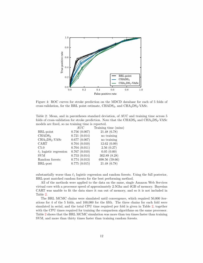
In Fig. 4 we give ROC curves for all 5 folds for BRL-point, CHADS2, and CHA2DS2-VASc, and in Table 2 we report mean AUC across the folds. These results show thatwith complexity and interpretability similar to CHADS2, the BRL point estimate decisionlists performed significantly better at stroke prediction than both CHADS2 and CHA2DS2-VASc. Interestingly, we also found that CHADS2 outperformed CHA2DS2-VASc despiteCHA2DS2-VASc being an extension of CHADS2. This is likely because the model for theCHA2DS2-VASc score, in which risk factors are added linearly, is a poor model of actualstroke risk. For instance, the stroke risk percentages calibrated to the CHA2DS2-VAScscores are not a monotonic function of score: The stroke risk with a CHA2DS2-VASc scoreof 7 is 9.6%, whereas a score of 8 corresponds to a stroke risk of 6.7% [Lip et al., 2010a].The fact that more stroke risk factors can correspond to a lower stroke risk suggests thatthe CHA2DS2-VASc model may be misspecified, and highlights the difficulty in constructingthese interpretable models manually.

The results in Table 2 give the AUC for BRL, CHADS2, CHA2DS2-VASc, along withthe same collection of machine learning algorithms used in Section 3.2. The decision treealgorithms CART and C5.0, the only other interpretable classifiers, were outperformedeven by CHADS2. The BRL-point performance was comparable to that of SVM, and not

11

0.0 0.2 0.4 0.6 0.8 1.0

False positive rate

0.0

0.2

0.4

0.6

0.8

1.0

Tru

epo

siti

vera

te

BRL-pointCHADS2

CHA2DS2-VASc

Figure 4: ROC curves for stroke prediction on the MDCD database for each of 5 folds ofcross-validation, for the BRL point estimate, CHADS2, and CHA2DS2-VASc.

Table 2: Mean, and in parentheses standard deviation, of AUC and training time across 5folds of cross-validation for stroke prediction. Note that the CHADS2 and CHA2DS2-VAScmodels are fixed, so no training time is reported.

AUC Training time (mins)BRL-point 0.756 (0.007) 21.48 (6.78)CHADS2 0.721 (0.014) no trainingCHA2DS2-VASc 0.677 (0.007) no trainingCART 0.704 (0.010) 12.62 (0.09)C5.0 0.704 (0.011) 2.56 (0.27)`1 logistic regression 0.767 (0.010) 0.05 (0.00)SVM 0.753 (0.014) 302.89 (8.28)Random forests 0.774 (0.013) 698.56 (59.66)BRL-post 0.775 (0.015) 21.48 (6.78)

substantially worse than `1 logistic regression and random forests. Using the full posterior,BRL-post matched random forests for the best performing method.

All of the methods were applied to the data on the same, single Amazon Web Servicesvirtual core with a processor speed of approximately 2.5Ghz and 4GB of memory. BayesianCART was unable to fit the data since it ran out of memory, and so it is not included inTable 2.

The BRL MCMC chains were simulated until convergence, which required 50,000 iter-ations for 4 of the 5 folds, and 100,000 for the fifth. The three chains for each fold weresimulated in serial, and the total CPU time required per fold is given in Table 2, togetherwith the CPU times required for training the comparison algorithms on the same processor.Table 2 shows that the BRL MCMC simulation was more than ten times faster than trainingSVM, and more than thirty times faster than training random forests.

12

Table 3: Mean, and in parentheses standard deviation, of AUC and training time (mins)across 5 folds of cross-validation for stroke prediction

Female patients Male patientsAUC Training time AUC Training time

BRL-point 0.747 (0.028) 9.12 (4.70) 0.738 (0.027) 6.25 (3.70)CHADS2 0.717 (0.018) no training 0.730 (0.035) no trainingCHA2DS2-VASc 0.671 (0.021) no training 0.701 (0.030) no trainingCART 0.704 (0.024) 7.41 (0.14) 0.581 (0.111) 2.69 (0.04)C5.0 0.707 (0.023) 1.30 (0.09) 0.539 (0.086) 0.55 (0.01)`1 logistic regression 0.755 (0.025) 0.04 (0.00) 0.739 (0.036) 0.01 (0.00)SVM 0.739 (0.021) 56.00 (0.73) 0.753 (0.035) 11.05 (0.18)Random forests 0.764 (0.022) 389.28 (33.07) 0.773 (0.029) 116.98 (12.12)BRL-post 0.765 (0.025) 9.12 (4.70) 0.778 (0.018) 6.25 (3.70)

4.1 Additional experiments

We further investigated the properties and performance of the BRL by applying it to twosubsets of the data, female patients only and male patients only. The female dataset con-tained 8368 observations, and the number of pre-mined antecedents in each of 5 folds rangedfrom 1982 to 2197. The male dataset contained 4218 observations, and the number of pre-mined antecedents in each of 5 folds ranged from 1629 to 1709. BRL MCMC simulationsand comparison algorithm training were done on the same processor as the full experiment.The AUC and training time across five folds for each of the datasets is given in Table 3.

The BRL point estimate again outperformed the other interpretable models (CHADS2,CHA2DS2-VASc, CART, and C5.0), and the BRL-post performance matched that of ran-dom forests for the best performing method. As before, BRL MCMC simulation requiredsignificantly less time than SVM or random forests training. Point estimate lists for theseadditional experiments are given in the supplemental materials.

5 Related Work

Most widely used medical scoring systems are designed to be interpretable, but are notnecessarily optimized for accuracy, and generally are derived from few factors. The Throm-bolysis In Myocardial Infarction (TIMI) Score [Antman et al., 2000], Apache II score forinfant mortality in the ICU [Knaus et al., 1985], the CURB-65 score for predicting mortalityin community-acquired pneumonia [Lim et al., 2003], and the CHADS2 score [Gage et al.,2001] are examples of interpretable predictive models that are very widely used. Each ofthese scoring systems involves very few calculations, and could be computed by hand duringa doctor’s visit. In the construction of each of these models, heuristics were used to designthe features and coefficients for the model; none of these models was fully learned from data.

In contrast with these hand-designed interpretable medical scoring systems, recent ad-vances in the collection and storing of medical data present unprecedented opportunitiesto develop powerful models that can predict a wide variety of outcomes [Shmueli, 2010].The front-end user interface of risk assessment tools are increasingly available online (e.g.,http://www.r-calc.com). At the end of the assessment, a patient may be told he or shehas a high risk for a particular outcome but without understanding why the risk is high or

13

what steps can be taken to reduce risk.In general, humans can handle only a handful of cognitive entities at once [Miller, 1956,

Jennings et al., 1982]. It has long since been hypothesized that simple models predictwell, both in the machine learning literature [Holte, 1993], and in the psychology literature[Dawes, 1979]. The related concepts of explanation and comprehensibility in statisticalmodeling have been explored in many past works [Bratko, 1997, Madigan et al., 1997,Giraud-Carrier, 1998, Ruping, 2006, Nowozin et al., 2007, Huysmans et al., 2011, Vellidoet al., 2012, Freitas, 2014, for example].

Decision lists have the same form as models used in the expert systems literature from the1970’s and 1980’s [Leondes, 2002], which were among the first successful types of artificialintelligence. The knowledge base of an expert system is composed of natural languagestatements that are if... then... rules. Decision lists are a type of associative classifier,meaning that the list is formed from association rules. In the past, associative classifiershave been constructed from heuristic greedy sorting mechanisms [Rivest, 1987, Liu et al.,1998, Li et al., 2001, Yin and Han, 2003, Marchand and Sokolova, 2005, Yi and Hullermeier,2005, Rudin et al., 2013]. Some of these sorting mechanisms work provably well in specialcases, for instance when the decision problem is easy and the classes are easy to separate,but are not optimized to handle more general problems. Sometimes associative classifiersare formed by averaging several rules together, but the resulting classifier is not generallyinterpretable [Friedman and Popescu, 2008, Meinshausen, 2010]. Chang [2012] orders rulesusing discrete optimization.

Decision trees are closely related to decision lists, and are in some sense equivalent: anydecision tree can be expressed as a decision list, and any decision list is a one-sided decisiontree. Decision trees are almost always constructed greedily from the top down, and thenpruned heuristically upwards and cross-validated to ensure accuracy. Because the trees arenot fully optimized, if the top of the decision tree happened to have been chosen badly atthe start of the procedure, it could cause problems with both accuracy and interpretability.Bayesian decision trees [Chipman et al., 1998, Dension et al., 1998, Chipman et al., 2002]use Markov chain Monte Carlo (MCMC) to sample from a posterior distribution over trees.Since they were first proposed, several improvements and extensions have been made inboth sampling methods and model structure [Wu et al., 2007, Chipman et al., 2010, Taddyet al., 2011]. The space of decision lists using pre-mined rules is significantly smaller thanthe space of decision trees, making it easier to obtain MCMC convergence. Moreover, rulemining allows for the rules to be individually powerful.

This work is related to the Hierarchical Association Rule Model (HARM), a Bayesianmodel that uses rules [McCormick et al., 2012]. HARM estimates the conditional probabili-ties of each rule jointly in a conservative way. Each rule acts as a separate predictive model,so HARM does not explicitly aim to learn an ordering of rules.

A theoretical work [Rudin et al., 2013] by the same authors provides guarantees onprediction quality for decision lists using statistical learning theory.

6 Discussion and Conclusion

We are working under the hypothesis that many real datasets permit predictive models thatcan be surprisingly small. This was hypothesized over a decade ago [Holte, 1993], however,we now are starting to have the computational tools to truly test this hypothesis. The BRLmethod introduced in this work aims to hit the “sweet spot” between predictive accuracy,

14

interpretability, and tractability.Interpretable models have the benefits of being both concise and convincing. A small

set of trustworthy rules can be the key to communicating with domain experts and to allowmachine learning algorithms to be more widely implemented and trusted. In practice, apreliminary interpretable model can help domain experts to troubleshoot the inner work-ings of a complex model, in order to make it more accurate and tailored to the domain.We demonstrated that interpretable models lend themselves to the domain of predictivemedicine, but there are a wide variety of domains in science, engineering, and industry,where these models would be a natural choice.

Appendix

Comparison algorithm implementations

Support vector machines: LIBSVM [Chang and Lin, 2011] with a radial basis function ker-nel. We selected the slack parameter CSVM and the kernel parameter γ using a grid searchover the ranges CSVM ∈ {2−2, 20, . . . , 26} and γ ∈ {2−6, 2−4, . . . , 22}. We chose the setof parameters with the best 3-fold cross-validation performance using LIBSVM’s built-incross-validation routine. C5.0 : The R library “C50” with default settings. CART : The Rlibrary “rpart” with default parameters and pruned using the complexity parameter thatminimized cross-validation error. Logistic regression: The LIBLINEAR [Fan et al., 2008]implementation of logistic regression with `1 regularization. We selected the regulariza-tion parameter CLR from {2−6, 2−4, . . . , 26} as that with the best 3-fold cross-validationperformance, using LIBLINEAR’s built-in cross-validation routine. Random forests: TheR library “randomForest.” The optimal value for the parameter “mtry” was found using“tuneRF,” with its default 50 trees. The optimal “mtry” was then used to fit a randomforests model with 500 trees, the library default. Bayesian CART : The R library “tgp,”function “bcart” with default settings.

Acknowledgement

Ben Letham and Cynthia Rudin were partly funded by NSF CAREER IIS-1053407 from theNational Science Foundation to C. Rudin. Tyler McCormick’s research was partially fundedby a Google Faculty Award and NIAID grant R01 HD54511. David Madigan’s research waspartly funded by grant R01 GM87600-01 from the National Institutes for Health. Theauthors thank Zachary Shahn and the OMOP team for help with the data.

References

Elliott M. Antman, Marc Cohen, Peter J.L.M. Bernink, Carolyn H. McCabe, Thomas Ho-racek, Gary Papuchis, Branco Mautner, Ramon Corbalan, David Radley, and EugeneBraunwald. The TIMI risk score for unstable angina/non-ST elevation MI: a method forprognostication and therapeutic decision making. The Journal of the American MedicalAssociation, 284(7):835–842, 2000.

K. Bache and M. Lichman. UCI machine learning repository, 2013. http://archive.ics.uci.edu/ml.

15

Christian Borgelt. An implementation of the FP-growth algorithm. In Proceedings of the1st International Workshop on Open Source Data Mining: Frequent Pattern Mining Im-plementations, OSDM ’05, pages 1–5, 2005.

I. Bratko. Machine learning: between accuracy and interpretability. In Giacomo Della Ric-cia, Hans-Joachim Lenz, and Rudolf Kruse, editors, Learning, Networks and Statistics,volume 382 of International Centre for Mechanical Sciences, pages 163–177. SpringerVienna, 1997. ISBN 978-3-211-82910-3. doi: 10.1007/978-3-7091-2668-4 10. URLhttp://dx.doi.org/10.1007/978-3-7091-2668-4_10.

Leo Breiman. Heuristics of instability and stabilization in model selection. The Annals ofStatistics, 24:2350–2383, 1996a.

Leo Breiman. Bagging predictors. Machine Learning, 24:123–140, 1996b.

Leo Breiman. Random forests. Machine Learning, 45:5–32, 2001.

Leo Breiman, Jerome H. Friedman, Richard A. Olshen, and Charles J. Stone. Classificationand Regression Trees. Wadsworth, 1984.

Allison Chang. Integer Optimization Methods for Machine Learning. PhD thesis, Mas-sachusetts Institute of Technology, 2012.

Chih-Chung Chang and Chih-Jen Lin. LIBSVM: a library for support vector machines.ACM Transactions on Intelligent Systems and Technology, 2:27:1–27:27, 2011. Softwareavailable at http://www.csie.ntu.edu.tw/~cjlin/libsvm.

Hugh A Chipman, Edward I George, and Robert E McCulloch. Bayesian CART modelsearch. Journal of the American Statistical Association, 93(443):935–948, 1998.

Hugh A Chipman, Edward I George, and Robert E McCulloch. Bayesian treed models.Machine Learning, 48(1/3):299–320, 2002.

Hugh A. Chipman, Edward I. George, and Robert E. McCulloch. BART: Bayesian additiveregression trees. The Annals of Applied Statistics, 4(1):266–298, 2010.

Robyn M Dawes. The robust beauty of improper linear models in decision making. AmericanPsychologist, 34(7):571–582, 1979.

D Dension, B Mallick, and A.F.M. Smith. A Bayesian CART algorithm. Biometrika, 85(2):363–377, 1998.

James Dougherty, Ron Kohavi, and Mehran Sahami. Supervised and unsupervised dis-cretization of continuous features. In Proceedings of the 12th International Conference onMachine Learning, ICML ’95, pages 194–202, 1995.

Rong-En Fan, Kai-Wei Chang, Cho-Jui Hsieh, Xiang-Rui Wang, and Chih-Jen Lin. LIB-LINEAR: a library for large linear classification. Journal of Machine Learning Research,9:1871–1874, 2008.

Usama M. Fayyad and Keki B. Irani. Multi-interval discretization of continuous-valuedattributes for classification learning. In Proceedings of the 1993 International Joint Con-ference on Artificial Intelligence, volume 2 of IJCAI ’93, pages 1022–1027, 1993.

16

Alex A Freitas. Comprehensible classification models: a position paper. ACM SIGKDDExplorations Newsletter, 15(1):1–10, 2014.

Jerome H. Friedman and Bogdan E. Popescu. Predictive learning via rule ensembles. TheAnnals of Applied Statistics, 2(3):916–954, 2008.

Brian F. Gage, Amy D. Waterman, William Shannon, Michael Boechler, Michael W. Rich,and Martha J. Radford. Validation of clinical classification schemes for predicting stroke.Journal of the American Medical Association, 285(22):2864–2870, 2001.

Andrew Gelman and Donald B. Rubin. Inference from iterative simulation using multiplesequences. Statistical Science, 7(4):457–472, November 1992.

Christophe Giraud-Carrier. Beyond predictive accuracy: what? In Proceedings of theECML-98 Workshop on Upgrading Learning to Meta-Level: Model Selection and DataTransformation, pages 78–85, 1998.

Robert C. Holte. Very simple classification rules perform well on most commonly useddatasets. Machine Learning, 11(1):63–91, 1993.

Johan Huysmans, Karel Dejaeger, Christophe Mues, Jan Vanthienen, and Bart Baesens.An empirical evaluation of the comprehensibility of decision table, tree and rule basedpredictive models. Decision Support Systems, 51(1):141–154, 2011.

Dennis L. Jennings, Teresa M. Amabile, and Lee Ross. Informal covariation assessments:data-based versus theory-based judgements. In Daniel Kahneman, Paul Slovic, and AmosTversky, editors, Judgment Under Uncertainty: Heuristics and Biases,, pages 211–230.Cambridge Press, Cambridge, MA, 1982.

William A. Knaus, Ellizabeth A. Draper, Douglas P. Wagner, and Jack E. Zimmerman.APACHE II: a severity of disease classification system. Critical Care Medicine, 13:818–829, 1985.

Cornelius T. Leondes. Expert systems: the technology of knowledge management and decisionmaking for the 21st century. Academic Press, 2002.

Vladimir I. Levenshtein. Binary codes capable of correcting deletions, insertions, and rever-sals. Soviet Physics Doklady, 10(8):707–710, February 1966.

Wenmin Li, Jiawei Han, and Jian Pei. CMAR: accurate and efficient classification based onmultiple class-association rules. IEEE International Conference on Data Mining, pages369–376, 2001.

WS Lim, MM van der Eerden, R Laing, WG Boersma, N Karalus, GI Town, SA Lewis,and JT Macfarlane. Defining community acquired pneumonia severity on presentation tohospital: an international derivation and validation study. Thorax, 58(5):377–382, 2003.

Gregory Y.H. Lip, Lars Frison, Jonathan L. Halperin, and Deirdre A. Lane. Identifyingpatients at high risk for stroke despite anticoagulation: a comparison of contemporarystroke risk stratification schemes in an anticoagulated atrial fibrillation cohort. Stroke,41:2731–2738, 2010a.

17

GY Lip, R Nieuwlaat, R Pisters, DA Lane, and HJ Crijns. Refining clinical risk stratificationfor predicting stroke and thromboembolism in atrial fibrillation using a novel risk factor-based approach: the Euro heart survey on atrial fibrillation. Chest, 137:263–272, 2010b.

Bing Liu, Wynne Hsu, and Yiming Ma. Integrating classification and association rulemining. In Proceedings of the 4th International Conference on Knowledge Discovery andData Mining, KDD ’98, pages 80–96, 1998.

D Madigan, K Mosurski, and RG Almond. Explanation in belief networks. Journal ofComputational and Graphical Statistics, 6:160–181, 1997.

David Madigan, Sushil Mittal, and Fred Roberts. Efficient sequential decision making algo-rithms for container inspection operations. Naval Research Logistics, 58:637–654, 2011.

Mario Marchand and Marina Sokolova. Learning with decision lists of data-dependentfeatures. Journal of Machine Learning Research, 6:427–451, 2005.

Tyler H. McCormick, Cynthia Rudin, and David Madigan. Bayesian hierarchical rule mod-eling for predicting medical conditions. The Annals of Applied Statistics, 6:652–668, 2012.

Nicolai Meinshausen. Node harvest. The Annals of Applied Statistics, 4(4):2049–2072, 2010.

George A. Miller. The magical number seven, plus or minus two: some limits to our capacityfor processing information. The Psychological Review, 63(2):81–97, 1956.

Sebastian Nowozin, Koji Tsuda, Takeaki Uno, Taku Kudo, and Gokhan Bakir. Weightedsubstructure mining for image analysis. In Proceedings of the 2007 IEEE Computer SocietyConference on Computer Vision and Pattern Recognition, CVPR ’07, 2007.

J. Ross Quinlan. C4.5: Programs for Machine Learning. Morgan Kaufmann, 1993.

Ronald L. Rivest. Learning decision lists. Machine Learning, 2(3):229–246, 1987.

Cynthia Rudin, Benjamin Letham, and David Madigan. Learning theory analysis for asso-ciation rules and sequential event prediction. Journal of Machine Learning Research, 14:3384–3436, 2013.

Stefan Ruping. Learning interpretable models. PhD thesis, Universitat Dortmund, 2006.

Galit Shmueli. To explain or to predict? Statistical Science, 25(3):289–310, August 2010.ISSN 0883-4237. URL http://dx.doi.org/10.1214/10-STS330.

Ramakrishnan Srikant and Rakesh Agrawal. Mining quantitative association rules in largerelational tables. In Proceedings of the 1996 ACM SIGMOD International Conference onManagement of Data, SIGMOD ’96, pages 1–12, 1996.

PE Stang, PB Ryan, JA Racoosin, JM Overhage, AG Hartzema, C Reich, E Welebob,T Scarnecchia, and J Woodcock. Advancing the science for active surveillance: ratio-nale and design for the observational medical outcomes partnership. Annals of InternalMedicine, 153:600–606, 2010.

Matthew A. Taddy, Robert B. Gramacy, and Nicholas G. Polson. Dynamic trees for learningand design. Journal of the American Statistical Association, 106(493):109–123, 2011.

18

Vladimir N. Vapnik. The Nature of Statistical Learning Theory. Springer-Verlag, New York,1995.

Alfredo Vellido, Jose D. Martın-Guerrero, and Paulo J.G. Lisboa. Making machine learningmodels interpretable. In Proceedings of the European Symposium on Artificial NeuralNetworks, Computational Intelligence and Machine Learning, 2012.

Xindong Wu, Chengqi Zhang, and Shichao Zhang. Efficient mining of both positive andnegative association rules. ACM Transactions on Information Systems, 22(3):381–405,July 2004.

Yuhong Wu, Hakon Tjelmeland, and Mike West. Bayesian CART: prior specification andposterior simulation. Journal of Computational and Graphical Statistics, 16(1):44–66,2007.

Yu Yi and Eyke Hullermeier. Learning complexity-bounded rule-based classifiers by com-bining association analysis and genetic algorithms. In Proceedings of the Joint 4th Inter-national Conference in Fuzzy Logic and Technology, EUSFLAT ’05, pages 47–52, 2005.

Xiaoxin Yin and Jiawei Han. Cpar: classification based on predictive association rules.In Proceedings of the 2003 SIAM International Conference on Data Mining, ICDM ’03,pages 331–335, 2003.

19

Supplement to “Interpretable classifiers using rules and Bayesian

analysis: Building a better stroke prediction model”

Benjamin Letham, Operations Research Center, Massachusetts Institute of Technology. bletham@mit.edu

Cynthia Rudin, Computer Science and Artificial Intelligence Laboratory, Massachusetts Institute ofTechnology. rudin@mit.edu

Tyler H. McCormick, Department of Statistics, Department of Sociology, Center for Statistics andthe Social Sciences, University of Washington. tylermc@u.washington.edu

David Madigan, Department of Statistics, Columbia University. madigan@stat.columbia.edu

This supplement provides the Bayesian Rule Lists (BRL) point estimates recovered from the five folds ofcross-validation on the full stroke-prediction experiment in Figs 1-5. Figs 6 and 7 give BLR point estimatesfrom the female-only and male-only experiments, respectively.

if hemiplegia and age>60 then stroke risk 58.9% (53.8% - 63.8%)else if cerebrovascular disorder then stroke risk 47.8% (44.8% - 50.7%)else if transient ischaemic attack then stroke risk 23.8% (19.5% - 28.4%)else if occlusion and stenosis of carotid artery without infarction then stroke risk 15.8% (12.2% - 19.6%)else if altered state of consciousness and age>60 then stroke risk 16.0% (12.2% - 20.2%)else if age≤70 then stroke risk 4.6% (3.9% - 5.4%)else stroke risk 8.7% (7.9% - 9.6%)

Figure 1: Decision list for determining 1-year stroke risk following diagnosis of atrial fibrillation from patientmedical history. The risk given is the mean of the posterior consequent, and in parentheses is the 95%credible interval. Obtained from the first of five folds of cross-validation.

1

if hemiplegia and cerebrovascular disorder then stroke risk 64.7% (59.6% - 69.6%)else if cerebrovascular disorder then stroke risk 44.5% (41.6% - 47.5%)else if hemiplegia then stroke risk 32.7% (23.8% - 42.2%)else if congestive cardiac failure and hydrocodone then stroke risk 9.9% (8.4% - 11.5%)else if transient ischaemic attack then stroke risk 30.5% (25.1% - 36.2%)else if age>70 then stroke risk 9.1% (8.3% - 10.0%)else stroke risk 4.0% (3.3% - 4.8%)

Figure 2: Stroke prediction decision list obtained from the second fold of cross-validation.

if hemiplegia and cerebrovascular disorder then stroke risk 61.7% (56.5% - 66.9%)else if cerebrovascular disorder then stroke risk 44.8% (41.8% - 47.8%)else if transient ischaemic attack then stroke risk 26.1% (21.7% - 30.7%)else if occlusion and stenosis of carotid artery without infarction then stroke risk 15.2% (11.8% - 18.9%)else if hemiplegia then stroke risk 37.8% (27.7% - 48.5%)else if age≤60 then stroke risk 3.5% (2.8% - 4.4%)else stroke risk 8.1% (7.4% - 8.8%)

Figure 3: Stroke prediction decision list obtained from the third fold of cross-validation.

if hemiplegia and cerebrovascular disorder then stroke risk 61.3% (56.2% - 66.3%)else if cerebrovascular disorder then stroke risk 44.5% (41.5% - 47.5%)else if sodium chloride and chronic obstructive pulmonary disease then stroke risk 10.6% (8.3% - 13.1%)else if transient ischaemic attack then stroke risk 27.6% (22.8% - 32.7%)else if hemiplegia then stroke risk 41.6% (30.9% - 52.7%)else if age≤60 then stroke risk 3.2% (2.4% - 4.1%)else stroke risk 8.2% (7.5% - 8.9%)

Figure 4: Stroke prediction decision list obtained from the fourth fold of cross-validation.

if hemiplegia and cerebrovascular disorder then stroke risk 64.5% (59.3% - 69.5%)else if cerebrovascular disorder then stroke risk 44.2% (41.2% - 47.2%)else if chronic obstructive pulmonary disease and chest pain then stroke risk 8.4% (7.2% - 9.8%)else if transient ischaemic attack then stroke risk 30.2% (24.8% - 35.8%)else if age≤60 then stroke risk 3.1% (2.3% - 4.0%)else if hemiplegia then stroke risk 44.6% (32.8% - 56.7%)else stroke risk 8.9% (8.1% - 9.7%)

Figure 5: Stroke prediction decision list obtained from the fifth fold of cross-validation.

2

if hemiplegia then stroke risk 59.0% (53.4% - 64.6%)else if cerebrovascular disorder then stroke risk 44.7% (41.2% - 48.3%)else if hypovolaemia and chest pain then stroke risk 14.6% (11.6% - 17.9%)else if transient ischaemic attack then stroke risk 29.9% (24.0% - 36.2%)else if age≤70 then stroke risk 4.5% (3.6% - 5.5%)else stroke risk 9.0% (8.0% - 10.0%)

Figure 6: Stroke prediction decision list obtained from the first fold of cross-validation on the females-onlydataset.

if hemiplegia and age>70 then stroke risk 57.6% (47.8% - 67.1%)else if transient ischaemic attack and chest pain then stroke risk 39.1% (31.6% - 46.9%)else if occlusion and stenosis of carotid artery without infarction and coronary artery arteriosclerosis thenstroke risk 21.1% (14.9% - 28.0%)else if cerebrovascular disorder then stroke risk 49.6% (43.8% - 55.5%)else stroke risk 6.8% (5.8% - 7.7%)

Figure 7: Stroke prediction decision list obtained from the first fold of cross-validation on the males-onlydataset.

3