From June 2009 QST © ARRL

There are many ham radio related activ-ities that provide a rich opportunity to explore and learn more about the sci-

ence of radio. One of those opportunities is radio astronomy.

All matter emits radio frequency (RF) energy dependent on the temperature and makeup of the matter, including the matter in space. The foundation of radio astronomy is to study the heavens by collecting and analyzing the RF energy that is emitted by bodies in space, very much as optical astronomers use light energy collected by telescopes. It sounds complicated. While professionals use very sophisticated and expensive equipment, you can, with some simple equipment and a little investment, build a radio telescope that will allow you to learn and explore the fundamentals of radio astronomy.

A Homemade Radio TelescopeIn this article, I will build on an existing

design of a radio telescope made from one of those ubiquitous TV dish antennas that you see around your neighborhood. The radio telescope (RT) project described here can easily be reproduced. Although this is not a fully capable RT, it can provide a wonder-ful learning opportunity for you, or perhaps students in your local school.

Figure 1 shows the radio telescope set up. The major components include a modified TV dish antenna mounted on a wooden sup-port structure to allow pointing the antenna, a commercial satellite signal strength detector that displays the signal strength of signals collected by the dish on a meter and an inter-face that converts the signal strength into a amplitude modulated tone. The tone is fed into a computer sound card and finally a computer and software graphically displays the signal strength as a function of time.

The TV dish modifications are structural, and any available TV dish system can be used. The signal strength detector costs between $40 and $65 and is widely available from Web retailers. The interface circuit, which will be described shortly, is easily duplicated and costs approximately $20. Finally, the display software is free.

Build a Homebrew Radio TelescopeExplore the basics of radio astronomy with this easy to construct telescope.

Mark Spencer, WA8SME

Figure 1 — Radio telescope system based on TV dish antenna.

Figure 2 — Dual LNB mount. Note two coax connectors.

Figure 3 — Homemade plastic single LNB mounting bracket.

  Measure the radiation intensity of the Sun and perhaps detect changes in solar activity. Measure the relative changes in the sur-

face temperature of the moon. Learn about and explore a common radio

astronomy collection technique called the drift scan.

What it Can DoThe following is just a sample of what

you can do with this simple RT: Use the sun to study and determine the

beamwidth of the dish and verify the mathematic formula that is used to predict dish antenna performance.

From June 2009 QST © ARRL

 Explore the fundamental principle of energy emission as a function of tempera-ture by detecting the relative differences between the temperatures of emitting bodies. Detect satellites parked along the Clarke

Belt in geosynchronous orbit and illustrate how crowded space has become. 1Notes appear on page 45.

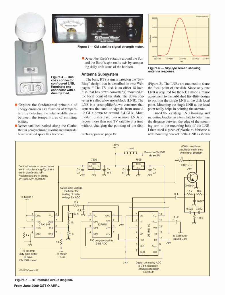
Figure 4 — Dual coax connector configured LNB. Terminate one connector with a dummy load.

Figure 5 — CM satellite signal strength meter.

Figure 6 — SkyPipe screen showing antenna response.

Figure 7 — RT Interface circuit diagram.

 Detect the Earth’s rotation around the Sun and the Earth’s spin on its axis by compar-ing daily drift scans of the horizon.

Antenna Subsystem The basic RT system is based on the “Itty-

Bitty” design that is described in two Web pages.1,2 The TV dish is an offset 18 inch dish that has down converter(s) mounted at the focal point of the dish. The down con-verter is called a low noise block (LNB). The LNB is a preamplifier/down converter that converts the satellite signals from around 12 GHz down to around 2.4 GHz. Most modern dishes have two or more LNBs to access more than one TV satellite at a time without changing the pointing of the dish

(Figure 2). The LNBs are mounted to share the focal point of the dish. Since only one LNB is required for the RT, I made a minor adjustment to the published Itty-Bitty design to position the single LNB at the dish focal point. Mounting the single LNB at the focal point really helps in pointing the antenna.

I used the existing LNB housing and mounting bracket as a template to determine the distance between the edge of the mount-ing arm to the mounting hole of the LNB. I then used a piece of plastic to fabricate a new mounting bracket for the LNB as shown

From June 2009 QST © ARRL

to digital converter (ADC). The variable resis-tor in this voltage multiplier circuit is used to calibrate the CM to SkyPipe. The voltage from the multiplier is fed to a programmable interface controller (PIC) that is programmed as a 9-bit ADC to covert the analog voltage that is a function of received signal strength to a 9-bit digital word that is used to control a digitally controlled variable resistor. The interface includes a simple Twin-T audio oscillator circuit that provides a tone of approximately 800 Hz that is fed to the com-puter sound card. The amplitude of this audio oscillator is varied by the digital pot that is being controlled by the PIC. The result is the audio amplitude being varied in step with the signal strength detected by the CM.

The circuit provides power to the CM and the LNB. A 12 V source in the CM is tapped through an RF choke and this is connected to the LNB coax connector inside the CM (Figure 9). The 12 V is also regulated to 5 V to provide power to the interface. Though prob-ably not required, there are two 5 V sources, one for the digital components of the interface, and the other for the analog components with one common ground point. This arrangement is used to isolate potential digital and analog noise sources within the circuit.

The interface is built on a circuit board and mounted right

inside the CM box

Figure 8 — RT Interface block diagram.

Figure 9 — Power and ground connection to CM board.

Figure 10 — CM with interface board.

in Figure 3. The dimensions are not super critical, but careful placement certainly will improve the RT performance.

Some LNBs have two coax connec-tors. Only one will be used in the RT (Figure 4). It is a good idea to terminate the extra coax connector with a 75 Ω dummy load plug to balance the load on the LNB. The dummy loads for F type TV coax con-nectors are readily available from electronic parts retailers.

Note that the dish is mounted upside down. Though this orientation is not ideal for receiving satellite signals, this arrange-ment helps with pointing the dish in its radio telescope role.

Satellite Detector The detector used in this project is the

Channel Master (CM) satellite signal level meter model 1004IFD (Figure 5).3 The CM is connected to the LNB. Power is supplied to the LNB through the coax connection from the CM. The CM detects the signal coming from the LNB and gives a meter indication of the signal strength and also varies the frequency of an audio tone to help technicians point the dish at the desired satellite. As you move the dish through the beam coming from the satellite, the meter indication will increase and then decrease coincident with the pitch of the audio tone.

The Itty-Bitty plans detail how to connect power to the CM and in turn connect power to the LNB (this power connection is han-dled by the interface in this project). Though somewhat effective, the CM meter and variable frequency tone indications provide limited utility in detecting changes in signal strengths required for radio astronomy.

Display To really study the signals received by

the RT, you will need to see them displayed graphically on a strip chart. There is an excellent software package called Radio-

SkyPipe that is posted on radio astronomy Web sites.4 The free version of this software is a good place to start. SkyPipe uses the computer sound card to measure the incom-ing signal strength and graphically displays the signal strength as a function of time. Figure 6 is illustrative of a signals detected by the RT. SkyPipe is very easy to use but some study of the HELP files will make it easier for you to fully tap into the capabili-ties of this software.

SkyPipe requires audio signals to be fed into the sound card MICROPHONE jack. The output of the CM detector is either an ana-log meter reading or a frequency modulated (constant amplitude) tone that is not really compatible with SkyPipe. An interface is required.

Interface What is required to make the CM output

work with SkyPipe and a sound card is to con-vert the signal level into an amplitude varying audio tone. The interface designed to do this is shown in Figure 7 and as a block diagram in Figure 8. Refer to the block diagram during the description of the interface function.

The unity-gain op-amp is used as a buf-fer between the CM meter driver circuit and the analog meter. The other op-amp is used as a voltage multiplier to scale the CM meter driver output voltage to match the 5 V reference voltage of the following analog

From June 2009 QST © ARRL

Figure 13 — Drift scan of the Sun indicating antenna’s azimuth pattern.

Figure 14 — Sequential drift scans. Note the time offsets between the peaks.

(Figure 10). Though I made an etched circuit board for the circuit, the hand wired pro-totype worked equally well for those who would rather roll their own. The PIC firm-ware is available on the QST Web site.6

RT in Action The first thing you need to do is learn

how to point the RT antenna. The best place

Figure 11 — Aiming the RT at the Sun, note LNB shadow location.

Figure 12 — Example calibration curves.

to start is to connect the CM to the antenna and point the antenna at the Sun. Caution: Do not look into the Sun as you do this, or at any time. Adjust the pointing angle and elevation until you get peak signal strength as indicated on the CM meter or hear the highest pitch audio tone. With the antenna pointed directly at the Sun, take note of the position of the shadow of the LNB on the surface of the dish (left in Figure 11). If you look from behind the dish, along the LNB

From June 2009 QST © ARRL

Figure 15 — Clarke Belt plot — tracking down satellites.

supporting arm (between the arm and the rim of the dish), you will see the Sun being blocked by the LNB.

Once you have the RT set up, it needs to be calibrated to match the output of the CM to SkyPipe. I have developed an Excel spreadsheet template to help with the cali-bration and a few of the other activities that you can accomplish with the RT (also avail-able from the QST Web site). Turn the RT to a signal source, the Sun, or the side of a building would work. Turn the gain control of the CM to set the meter to maximum. Run SkyPipe and adjust the variable resistor on the interface board until you get a read-ing on the SkyPipe graph vertical (y) axis of approximately 32,000. With the maxi-mum value set, adjust the CM gain control through the voltage range (0 to 100 mV) in 10 mV steps and record the corresponding y axis value on SkyPipe. This data is entered into the Excel spreadsheet to compute the calibration curve between voltage and y axis value. Both voltage and y axis values are used in analyzing recorded signal strength data (Figure 12).

A good first activity is to do a drift scan of the Sun. A drift scan means that you set the antenna azimuth (AZ) and elevation (EL) to some fixed pointing angle and allow the Earth to serve as the rotator to drag the antenna across the sky. To do a drift scan of the Sun, first set the elevation and azimuth to point directly at the Sun (maximum signal) and then move the azimuth toward the west

(leave the elevation set) until you are off the peak signal. Now start SkyPipe. In about 15 minutes, the Sun will pass through the antenna pattern beam width and the result will be as illustrated in Figure 13. You can also use this collection technique to explore the antenna performance parameters.

A good second activity is to do two drift scans of the night sky on two consecutive nights (beginning the scans at the same time each night) using the same fixed antenna azimuth (AZ) and elevation (EL). Figure 14 shows two such drift scans. Although at first glance they may not seem similar, there are some interesting features that are pointed to by arrows. If you compare the time that these two peaks occurred, the time differ-ence is about 4.5 minutes. This shift is the result of the distance the Earth had traveled during the 24 hours between collections.

This illustrates that the Earth’s rotation as well as its travel in orbit needs to be consid-ered when comparing drift scans. Enough to make your head spin (pun intended)?

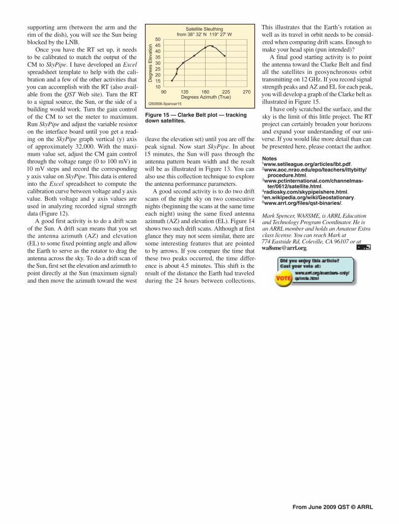
A final good starting activity is to point the antenna toward the Clarke Belt and find all the satellites in geosynchronous orbit transmitting on 12 GHz. If you record signal strength peaks and AZ and EL for each peak, you will develop a graph of the Clarke belt as illustrated in Figure 15.

I have only scratched the surface, and the sky is the limit of this little project. The RT project can certainly broaden your horizons and expand your understanding of our uni-verse. If you would like more detail than can be presented here, please contact the author.

Notes1www.setileague.org/articles/lbt.pdf.2www.aoc.nrao.edu/epo/teachers/ittybitty/

procedure.html.3www.pctinternational.com/channelmas-

ter/0612/satellite.html.4radiosky.com/skypipeishere.html.5en.wikipedia.org/wiki/Geostationary.6www.arrl.org/files/qst-binaries/.

Mark Spencer, WA8SME, is ARRL Education and Technology Program Coordinator. He is an ARRL member and holds an Amateur Extra class license. You can reach Mark at 774 Eastside Rd, Coleville, CA 96107 or at wa8sme@arrl.org.