Bubbles and fads in the stock market:another look at the experience of the US.

Piergiorgio Alessandri�

December 28, 2004

AbstractThis paper considers a standard present-value equity price formula

with time-varying discount rates, and proposes a state-space formula-tion that allows a decomposition of price �uctuations into fundamen-tal and non-fundamental components. By "fundamentals" we refer todividends, interest rates and risk premia, both actual and expected;the "non-fundamental" price component is de�ned residually allowingfor the possibility of a rational bubble.The empirical application uses annual US data, postulating a sim-

ple discount factor driven by the real return on short-term public debt.The stochastic factor explains part of the volatility in prices, but itis not su¢ cient to exclude the occurrence of near-exponential bubblesanalogous to those found in the constant discount literature. On thecontrary, de�nition and measurement of the fundamentals, and par-ticularly of the dividend payout, prove to be crucial in this respect.

�Birkbeck College, University of London; p.alessandri@econ.bbk.ac.uk. I wish tothank John Dri¢ ll for support and supervision, Pedro Bação, Ron Smith andMartín Solá for advice and comments, Robert Shiller and Stephen Wright formaking their datasets available. I am responsible for any remaining mistakes.Financial support from the ESRC (grant PTA-030-2002-00377) and the Journal ofApplied Econometrics is also gratefully acknowledged.

1

1 Introduction.

Was there a bubble in the nineties? The behaviour of the US stock marketin the last ten years has been exceptional in many respects. In the post-war period, the value of equity �uctuated between 40% and 100% of thegross domestic product. Between 1995 and 2000 the stock market capital-isation increased from 100% to 180%; by the end of 2002 it was back toroughly 120%. A cursory glance at the price-dividend and price-earningsratios delivers the same, simple message: prices were "unusually high" for afew years, and then suddenly reverted to more "normal" levels. Some ana-lysts attempted an explanation of these facts on the basis of fundamentalsonly. It has been suggested that once the dividend is replaced by a moresophisticated measure of the net cash�ow generated by the �rms, the behav-iour of the market appears to be consistent with some version of the classicGordon (1962) model (Robertson and Wright 2003, Wright 2004). Othersadmit that the decade was extraordinary, but explain it by pointing to ex-traordinary structural conditions. High prices may have been determined forinstance by �rms accumulating large stocks of intangible capital (e.g. Hall,2001) or by the baby-boom cohort saving for retirement (Geanakoplos et al.,2002). These models maintain that shares are priced according to a present-value formula, and that all low-frequency market movements are driven byobserved or expected changes in fundamentals. A common criticism is that,even when they convincingly explain the price runup, these theories are silenton the causes of the subsequent slump.

The alternative is to consider non-fundamental explanations, namely de-partures from the present-value pricing principle. Not surprisingly, the ninetiesrevived the interest for price bubbles on the media and in the academic litera-ture: the observed boom-and-bust cycle is in a way easier to rationalize afteraccepting the idea that price changes are not always related to changes in thepresent value of rationally forecasted future dividends. This line of investi-gation presents of course its own di¢ culties. Rational, self-ful�lling bubblescan be ruled out in many contexts by some backward induction argument,and speculative phenomena of a non-rational nature are di¢ cult to model ina non-arbitrary way. Furthermore, the empirical investigation has not pro-duced clear answers on the existence and nature of price misalignments, andmany factors suggest that the task is intrinsically very di¢ cult.This paper proposes a strategy to detect equity price misalignments, and

2

presents an empirical application based on US data. The next section surveysthe literature on bubbles, focussing on the empirical research. In section 3we discuss a general framework that allows to test for bubbles under di¤erentassumptions on the nature of the stochastic discount factor. The key compo-nent of the model is a linearised price formula obtained by a �rst order Taylorapproximation around the unconditional mean of the discount factor (Shiller(1981), Poterba and Summers (1986), West (1987)). The approximation canbe used to model prices, fundamentals and bubbles in a state-space frame-work, which allows maximum likelihood estimation of the bubble throughthe Kalman �lter (Burmeister and Wall (1982), Wu (1995, 1997), Chen etal. (2001)). An original feature of the model is that, due to the stochasticdiscount factor, the rate of growth of the bubble changes over time.

Section 4 examines the implications of the model when (i) agents discounton the basis of a safe return R(t) augmented by a constant risk premium,(ii) R(t) follows a stationary autoregressive process of order one and (iii)dividends are expected to grow at a constant rate. The main prediction ofthe model is a negative linear relationship between the price-dividend ratioand the safe rate, the strength of which depends on the persistence of theshocks to R(t). If the shocks are persistent, a high R(t) is expected to befollowed by a period of high rates, or low discount factors, which lowersthe contemporaneous price-dividend ratio. The model is estimated on threedi¤erent sets of annual observations on the US stock market. We use aStandard&Poors dataset, a non-�nancial industry dataset, and an adjustednon-�nancial industry dataset where the dividend is computed netting outnew share issues and buybacks. The safe return R(t) is taken to be the realrate on short-term public debt. In section 5 we compare the explanatorypower of the exponential bubble to that of the �intrinsic�bubble proposedby Froot and Obstfeld (1991). Section 6 concludes.

Our results can be summarised as follows. The assumption on the dis-count factor holds in all datasets; the interest rate has a signi�cant nega-tive impact on the price-dividend ratio, which also con�rms that there is amonetary policy channel operating through the stock market. We estimatesigni�cant bubbles in two datasets out of three: the S&P price index and,to a smaller extent, the non-adjusted industry share price are in�ated byspeculation in the sixties and late ninenties. In both cases, exponential bub-bles with time-varying rates of growth �t the data better than the intrinsic

3

bubble. There is no evidence of bubbles in the adjusted dataset.The analysis suggests two conclusions. Firstly, stochastic discount factors

and rational bubbles may well coexist. It is known that US equity prices ap-pear to be "too volatile" even after accounting for time variation in interestrates (Campbell and Shiller (1988), West (1988)); our work shows that spec-ulative bubbles are indeed a plausible explanation for the excess volatility.Secondly, measurement issues are crucial: a price-dividend ratio adjusted fornew issues and buybacks is clearly incompatible with bubbles, be them ex-trinsic or intrinsic. This is a strong incentive to think more carefully aboutwhich fundamental the agents consider when evaluating shares.

2 Testing for bubbles.

The theoretical conditions under which rational, self-ful�lling bubbles canarise are known (Blanchard and Watson (1982), Tirole (1982, 1985), Stiglitz(1990), LeRoy (2004) among others). Bubbles cannot occur in a �nite-horizon economy, or in an economy with a �nite number of in�nitely livedtraders. In a deterministic overlapping generations model, the bubble canonly arise if there are dynamic ine¢ ciencies leading to over-accumulation ofcapital. If the economy is e¢ cient, the bubble will eventually exceed thevalue of all available resources; as long as the agents are aware of this poten-tial inconsistency, bubbles can again be ruled out by a backward inductionargument1. Other departures from the present-value formula are possible.Price misalignments may occur due to the existence of "noise traders" whodo not behave in a fully rational way (Black (1986), Abreu and Brunner-meier (2003)). The misalignment, or fad, is then the di¤erence between theactual price and the price that would be observed if all traders were rational.Since this will be in general a mean-reverting process, in this case there areno long-run consistency issues. Though, a limit of this literature is that thebehaviour of noise traders is often taken as given or modelled relying on adhoc assumptions.

1This type of awareness is widely assumed but not completely uncontroversial. LeRoy(2004) suggests that agents who by de�nition never experienced a model failure may notappreciate the di¤erence between a consistent and an inconsistent path - which wouldmake the latter as likely as the former.

4

A large literature stimulated by Shiller (1981) and LeRoy and Porter(1981) has shown that equity prices are too volatile to be consistent witha constant discount present-value formula. Models with stochastic discountfactors linked to interest rates, consumption growth or variance of marketreturns attenuate the problem but do not solve it completely: a substan-tial portion of the variance of the price-dividend ratio remains unexplained(Poterba and Summers (1986), Campbell and Shiller (1988), West (1988)).Bubbles and fads are a potential explanation for the excess volatility, butany attempt to test this hypothesis faces a basic conceptual di¢ culty: pricemovements can in principle be rationalised by misalignments or by omitted"fundamental" state variables (Hamilton and Whiteman (1985), Flood andHodrick (1990)).

It is possible to test for price misalignments without relying on a speci�cparametrisation of the misalignment itself. West (1987) notes that the dis-count factor can be estimated from a one-period arbitrage equation or fromits forward solution, under some assumption on the process used to forecastdividends. If there is no bubble, the estimates should coincide. With a ratio-nal bubble, the estimates should diverge because the �rst equation holds butthe second omits a variable. Hence, a test on the two set of estimates beingequal is a test of the null that there is no bubble. The author uses annualUS data and rejects the null that there are no bubbles under several alterna-tive speci�cations of the dividend process. Chirinko and Shaller (1996, 2001)apply an analogous idea to Tobin�s Q investment model; in this case theEuler and equilibrium equations describe the optimal investment policy of arepresentative �rm. They �nd evidence of bubbles in the US and in Japan2.

Blanchard et al. (1993) and Bond and Cummins (2001) ask whetherdeviations of equity prices from fundamentals can be responsible for thetypically poor empirical performance ofQ investment equations. Both paperscompare a stock market measure of Q with one computed on the basis offundamentals. Blanchard et al. (1993) use annual aggregate US data and�nd that, if the equation contains a "fundamental Q" based on pro�ts, the

2These tests have some limitations. Any misalignment other than a rational bubblecauses the failure of both the Euler and the equilibrium equation, which in theory in-validates the procedure. An exponential rational bubble would on the other hand a¤ectthe distribution of the test statistic and possibly make the test inconsistent (West (1987),Chirinko and Shaller (2001)). Finally, the procedure may fail to detect bubbles if theseare completely uncorrelated with fundamentals.

5

marginal explanatory power of the market-related variable is negligible. Theconclusion is that misalignments are small and/or �rms ignore them. Bondand Cummins (2001) use data on a panel of American �rms, and measure Qrelying on published earnings forecasts; this variable appears to be a su¢ cientstatistic for investment and delivers plausible estimates of the adjustmentcost parameters. The authors infer that the Q model is correct, but itsparameters cannot be identi�ed using stock market data because share pricesdepart persistently from their fundamental level.Sarno and Taylor (1999) show that, if there is no rational bubble, the log

dividend-price ratio and the log ex post return must be either stationary orcointegrated (that is, time-variation in returns may imply the failure of the�rst condition, but not of the second). They analyse monthly stock marketdata for eight East Asian countries over the nineties; non-stationarity andlack of cointegration cannot be rejected for any of them, suggesting that assetprices were bubbly at the outset of the 1997 crisis.

It is also possible to test a speci�c bubble parametrisation. Flood andGarber (1980) develop a test for a monetary model of the German hyperin-�ation considering a deterministic bubble growing at a constant rate. Theidea is to test the signi�cance of an exponential time trend in a reduced-form in�ation equation. The no-bubble hypothesis is not rejected, but theprocedure raises some methodological issues (Flood and Hodrick (1990)); inparticular, because of the explosive regressor the authors�statistical infer-ence cannot rely on the standard asymptotic distribution theory. Flood etal. (1984) replicate a similar analysis exploiting a cross-sectional dimensionto by-pass this issue, and reject the null; the problem in this case lies withthe sample size, as only three simultaneous hyperin�ations are considered.In Froot and Obstfeld (1991) the bubble is a power of the contemporaneousdividend, which is assumed to follow a logaritmic random walk. The bubbleis thus completely deterministic and it is "intrinsic" in that all of its vari-ability stems from economic fundamentals. Using aggregate annual US dataup to 1988, the authors �nd that the price-dividend ratio is indeed positivelycorrelated to some power of the dividend. This paper is discussed in greaterdetail in section 5.

Finally, a few papers introduce a parametric bubble process in a state-space model, as we do here. The bubble, a non-observable state variable,can then be estimated by maximum likelihood through a Kalman �lter pro-

6

cedure. Burmeister and Wall (1982) pioneered this technique on the Germanhyperin�ation data, Wu (1995) and Elwood et al. (1999) apply it to exchangerates; Wu (1997) and Chen et al. (2001) use it to analyse the US equity mar-ket. Wu (1997) assumes a constant discount factor and models prices usingCampbell and Shiller�s (1988) log-linear approximation, �nding signi�cantevidence of bubbles. Chen et al. (2001) assume that the discount factor isdriven by an autoregressive risk premium and linearize the price around themean discount factor; they do not reject the no-bubble hypothesis. Thesetwo papers are clearly close in spirit to ours, and they are discussed moreextensively below.

3 A state-space formulation for the price ofa share.

This section introduces a linear approximation for a standard present-valueequity price formula with time-varying discount factor, and discusses the useof the approximation as a building block for a state-space formulation ofthe price process. The main references are Poterba and Summers (1986),that �rstly proposed the approximation3, Campbell and Shiller (1988), thatintroduced an alternative well-known logaritmic formula, and �nally Chen etal. (2001) andWu (1997), where these approximations are used to investigateequity price bubbles. It is well known after Lucas (1978) that, under riskneutrality, the current price of a share is the discounted value of the streamof expected dividends it will generate in the inde�nite future:

P ft = Et

1Xi=0

�i+1Dt+i (1)

(the superscript f stands for "fundamental"). It has been argued that theassumption of a constant discount factor � is a straightjacket to be avoided.A more general alternative is given by the following formula:

P ft = Et

1Xi=0

iYj=0

(1 + rt+j + �t+j)�1

!Dt+i (2)

3Analogous formulae appear in Shiller (1981), Abel and Blanchard (1986), West (1987).

7

The discounting is based here on a time-varying factor driven by thedynamics of a risk-free rate of return rt+j and a risk premium �t+j. Equation(2) is the no-bubble forward solution for the price of a share satisfying thecondition (EtPt+1�Pt)=Pt+Dt=Pt = rt+ �t; if no assumption is made aboutthe terms on the right-hand side, this is of course a mere accounting identitywithout a precise economic meaning. Poterba and Summers (1986) assumea constant interest rate r and develop a �rst order Taylor approximation of(2) around the mean risk premium

_� � E�t. A more �exible model can

be obtained by using a bivariate approximation. Assume that the safe rateand the premium have a �nite unconditional mean E(rt; �t) � (�r; ��). Theexistence of this moment is crucial: none of the equations below holds if,for instance, one of these variables is not covariance-stationary. If the meanexists, we can de�ne an "average" discount factor4 � � 1=(1 +

_r +

_�). A

�rst-order Taylor approximation of P ft (Dt+i; rt+i; �t+i) around Pft (Dt+i; �r; ��)

delivers the following equation:

P ft ' PLt +Rt + At (3)

where:

PLt �1Xi=0

�i+1EtDt+i (4)

At �1Xi=0

("��i+1

1Xk=0

�k+1EtDt+i+k

#(Et�t+i �

_�)

)(5)

Rt �1Xi=0

("��i+1

1Xk=0

�k+1EtDt+i+k

#(Etrt+i �

_r)

)(6)

Details on the derivation and the assumptions under which we can expectit to be accurate can be found in the appendix. The �rst term has beennamed PLt because it represents in a sense a "Lucas�price" - the dividendstream discounted on the basis of a constant factor �. The second and thirdterms show how expected deviations of risk premium and interest rates fromtheir equilibrium values in�uence today�s equity valuation. The fact thatAt and Rt contain products between dividends and deviations of �t and rt

4Because of the non-linearity of the relationship, this does not coincide with the un-conditional mean of the stochastic discount factor - hence the inverted commas.

8

from their means has a natural interpretation: the impact on today�s priceof an expected change in the discount factor at any future date depends onhow big is the cash�ow to be discounted from that date onwards. If forinstance agents believe that dividends will be zero after t + i�, for all i > i�the expression in square brackets is zero and the corresponding terms dropout of At and Rt: the price of the share today is thus independent of anyexpected movement in the discount factor after t+i�. If the misalignmentMt

is de�ned residually as the non-fundamental price component, we can write:

Pt � P ft +Mt ' PLt +Rt + At +Mt (7)

This is a candidate for the measurement equation in the state-spacemodel. The question is whether the right-hand side terms provide a setof suitable states.

PLt does not pose particular problem. As Hansen and Sargent (1980)�rstly showed, if Dt � AR(q) then PLt will be itself a linear function of q lagsof the dividend. By vectorising the autoregressive Dt process into a VAR(1)of dimension q, the �rst block of states can be written as follows:0BB@

Dt+1

Dt

:::Dt�q+2

1CCA =

2664�00:::0

3775+2664�1 �2 ::: �q1 0 ::: 0

::: :::0 ::: 1 0

37750BB@

Dt

Dt�1:::

Dt�q+1

1CCA+0BB@"t+10:::0

1CCA (8)

Hansen and Sargent�s result implies PLt = c0(�; �)+Pq

i=1 ci(�; �)Dt�i+1 ,where each ci is a known function of �i i = 0; :::; q and �.

At and Rt are less straightforward. Chen et al. (2001) show that At (Nt intheir notation) follows an AR(1) process with a time-varying intercept and aninnovation that is a complicated function of conditional moments of Dt+i and�t+i. Since an analogous equation holds for Rt, one possibility is to modelAt and Rt as non-observable state variables. However, this procedure failsto impose some cross-equation restrictions and introduces two error termsthat are well-behaved only under extra assumptions on the data-generatingprocess. Again, a discussion of these issues is presented in the appendix. Thenext section shows that fortunately, despite the apparent cumbersomeness of

9

equations (5) and (6), Rt and At turn out to be reasonably simple functionsof Dt; rt and �t in a range of economically interesting cases. Therefore, thesystem can be directly speci�ed in terms of dividends, interest rates and riskpremia without introducing any further variable.

As far as Mt is concerned, a completely agnostic approach would requirenot taking a stance on the nature of the misalignment. On the other hand,if Mt is simply considered part of the price equation error term, the occur-rence of a serially correlated rational bubble could invalidate the model. Thesolution is to allow for both a rational bubble and a purely random devia-tion from fundamentals: Mt = Bt + nt, where n denotes a "noise" satisfyingE(nt) = 0 for all t and E(ntns) = 0 for all t 6= s. The bubble is modelled asa further non-observable forcing state:

Bt+1 = (1 + rt + �t)Bt + bt+1 (9)

(where bt is a serially uncorrelated error term). Equation (9) generalises thestandard parametrisation of a rational bubble to the case where the discountfactor, and consequently the growth rate of the bubble, changes over time.This non-linearity makes the model more interesting because it allows theexamination of bubbles that roam about more irregularly than the usual,monotonically explosive variable examined by constant discount models. Aswe will show, there is no cost in terms of econometric complications as longas rt and �t can be observed. Note that the presence of nt and bt impliesthat both the measurement equation for Pt and the bubble are stochastic;the Kalman �lter is run under the assumption that the contemporaneous co-variance between the two error terms is zero. The nt factor can be interpetedas the consequence of fads or measurement errors.

We conclude the section relating this work to the log-linear approximationof Campbell and Shiller (1988). Both approximations are based on the de�ni-tion of return. Campbell and Shiller (1988) start from (Pt+1+Dt)=Pt = 1+Rt,take the logaritm of the identity and then compute a �rst order Taylor ap-proximation around the mean of the log dividend-price ratio �t � dt�1 � pt.By contrast, we write the ex ante return as the sum of a safe rate and a riskpremium, solve forward for the price level and then approximate the solution.The formulae in Campbell and Shiller (1988) have a clear advantage in termsof elegance and intuitive appeal; furthermore, they are linear in logaritms ofprices and dividends, so they can be combined with log-linear models that

10

seem to �t the data better and explicitly take into account the non-negativityof these variables. Our defense on this issue is twofold. Firstly, equation (8)is meant to be an empirical approximation of the process investors use toforecast dividends rather than a description of the "true" process. Sincedividends are positive and increase over time, the probability (8) attachesto the event fDt < 0g is small and approaches zero asymptotically; in thisrespect, the di¤erence between modelling the dividend in levels or in log-aritms is unlikely to be important. Secondly, the approximation and theimplied state-space system can be derived also under the assumption thatthe log-dividend follows a random walk5.

There are two more substantial di¤erences. Campbell and Shiller (1988)approximate around the mean log dividend-price ratio E(�t). If there is abubble, this moment does not exist: prices may inde�nitely diverge fromdividends, pushing the dividend-price ratio to zero and its logaritm to mi-nus in�nity. Since the approximation is only valid under the null that thereare no bubbles, it should not be used to test for their existence. On thecontrary, the mean discount factor is well-de�ned independently of the exis-tence of bubbles. A related issue is the accuracy of the linearisations. Camp-bell and Shiller�s (1988) formula holds exactly if the dividend yield is con-stant (�t = �), whereas ours holds exactly if the discount factor is constant(rt + �t = r + �); the approximation errors respectively depend on the un-conditional volatility of these variables. Poterba and Summers (1986) do notdiscuss the accuracy of their formula; numerical analysis is probably the onlyway to gain insight on the relative quality of the two approximations. How-ever, the real interest rate is typically less volatile than the log dividend-priceratio, and the nineties have seriously weakened the evidence on the station-arity of the latter. Bubbles may or may not be responsible for this, but as amatter of fact the yield appears to depart persistently from its mean level.Hence, provided the risk premium does not vary much, it may be in principlea good idea to approximate around the discount factor.

The second di¤erence has to do with the degree of generality of the mod-els. Campbell and Shiller (1988) can only allow for one source of randomnessin discounting. Their paper analyses four possibile speci�cations for the dis-

5In this case the state equation would be speci�ed with log(Dt) and the measurementequation would contain an exponential term Dt = e

log(Dt); again, the non-linearity can behandled easily because the dividend (or its logaritm) is an observable state.

11

count rate, respectively based on a constant, the real return on short-termdebt, the growth rate of real aggregate consumption and the variance of stockreturns. In all cases, either the safe return or the risk premium (or both) areconstant; this is unavoidable, because the equation only contains the overalldiscount factor. With the approximation used in this paper interest ratesand risk premia can be modelled separately. Since safe return and risk pre-mium are fundamentals that move under the in�uence of di¤erent forces, thedevelopment of econometric frameworks where they can be modelled inde-pendently is an important enterprise. The hope is that this work will give acontribution in that direction, despite the fact that in the simple applicationpresented in the next section, the premium is again assumed to be constant6.

4 A tentative model.

Equations (4)-(6) and (9) may be regarded as the basis for the speci�cationof simpler pricing models. The structure of each speci�c model will dependon the assumptions we are willing to make on dividends, interest rates andrisk premia, which in turn have to be consistent with the dataset at hand.The application proposed here is designed for a set of low-frequency (possiblyannual) aggregate data. For the time being, ignore the bubble process andconsider the case where:

i. Dt = �Dt�1 + "tii. rt = �0 + �1rt�1 + �tiii. �t = �

Dividends are expected to grow at a constant rate, the interest rate followsan autoregressive process of order one and the risk premium is constant; "tand �t are zero-mean, serially uncorrelated disturbances. These assumptionsare discussed in the appendix; here we just note that the analysis has thesame basic implications if (i) is replaced by the commonly used assumptionthat log(Dt) follows a random walk, and that (iii) could also be augmentedby an error term without consequences, because all we need is a process forwhich the unconditional mean is also the best conditional predictor at allhorizons (Et�t+i = E�t = �). With � > 1, two su¢ cient conditions in order

6If a simpli�cation has to be introduced, a constant risk premium is in our view moreappropriate than a constant safe rate of return. In the appendix we discuss this choicetogether with the alternative proposed by Chen et al. (2001).

12

for the series of conditional expectations in (4), (5) and (6) to be de�ned are�� < 1 and j�1j < 1. Under these assumptions we have EtDt+i = �

iDt andEt(rt+i� �r) = �i1(rt� �r), with �r = �0=(1� �1), which substantially simpli�esthe three equations:

PLt =�

1� ��Dt (10)

Rt =

��0

1� �1�2

1� ��1

1� ���1

�Dt �

��2

1� ��1

1� ���1

�Dtrt (11)

At = 0 (12)

It is clear now that the dynamics of Rt are dictated by those of theunderlying forcing states Dt and rt, and that there is no need to specify atransition equation for this variable. The transition equation (8) is replacedby (i) and, using the expressions above and collecting the two Dt terms, theprice equation (3) becomes:

P ft ' �

1� ��

�1 +

�01� �1

�

1� ���1

�Dt �

��2

(1� ��) (1� ���1)

�Dtrt

� c0Dt + c1Dtrt (13)

This equation has two simple implications. The �rst one is that the meanprice-dividend ratio also depends on the parameters of the process drivingthe discount factor: E(P ft =Dt) = c0 + c1�r. A simple algebraic manipulationshows that, for positive values of �0 and �1, this mean value is the productof the coe¢ cient implied by a constant discount model (�(1 � ��)�1) by anumber larger than one. The di¤erence between the two is small as long asthe mean safe rate �r is small. More importantly, dividend and interest rateinteract. The interaction e¤ect has a negative sign, meaning that coeterisparibus an increase in rt depresses prices, and its magnitude depends on�1, the persistence of the innovations in the interest rate process. If �1 islarge, a positive shock to rt has to be followed by a prolonged period ofhigh returns and low discount rates, and this is re�ected in a strong negativecorrelation between price and interest rate at time t. It is an interestingresult, because basically the equation contains an "extra" term that depends

13

on the contemporaneous dividend and, contrary to the intrinsic bubble ofFroot and Obstfeld (1991), does not have a speculative nature. The equationcan be re-cast for the price-dividend ratio:

PtDt

= c0 + c1rt + n�t (14)

where n�t = nt=Dt. Note that the system given by (i),(ii) and (13) imposestwo non-linear restrictions on �. We may now reintroduce the non-observablebubble by embedding the price equation into a fully speci�ed state-spacesystem:

Pt =�c0 c1 1

� �Dt Dtrt Bt

�0+ nt (15)

0@ Dt

rtBt

1A =

24 0�00

35+24 � 0 00 �1 00 0 (1 + rt�1 + �)

350@ Dt�1rt�1Bt�1

1A+0@ "t�tbt

1A (16)

The system has one measurement variable (Pt) and three state variables,two of which (Dt; rt) are observed. The measurement equation can alter-natively be speci�ed in terms of the price-dividend ratio by simply divingthrough by Dt. In either case, the system contains two non-linear elements:one in the measurement equation (either a product or a ratio of variables)and one in the transition equation for the bubble (because of the time-varyingrate of growth). These do not pose particular problems because Dt and rtare observable, i.e. they are known with certainty at time t; and the transi-tion matrix is diagonal. Another way of looking at it is that, since the onlyhidden state is Bt, we may simply formulate a system of a price equation anda bubble equation, considering Dt and rt "exogenous"; such a state-space isconditionally linear and it allows consistent maximum likelihood estimationof the parameters and minimum mean-squared error �ltering of the bubble(Harvey (1989)). An advantage of estimating a two-equations system forPt=Dt and Bt is that no assumption has to be made on the distribution ofthe error term in the dividend equation; the cost is clearly that it is notpossible to impose the restrictions on the ci coe¢ cients.

14

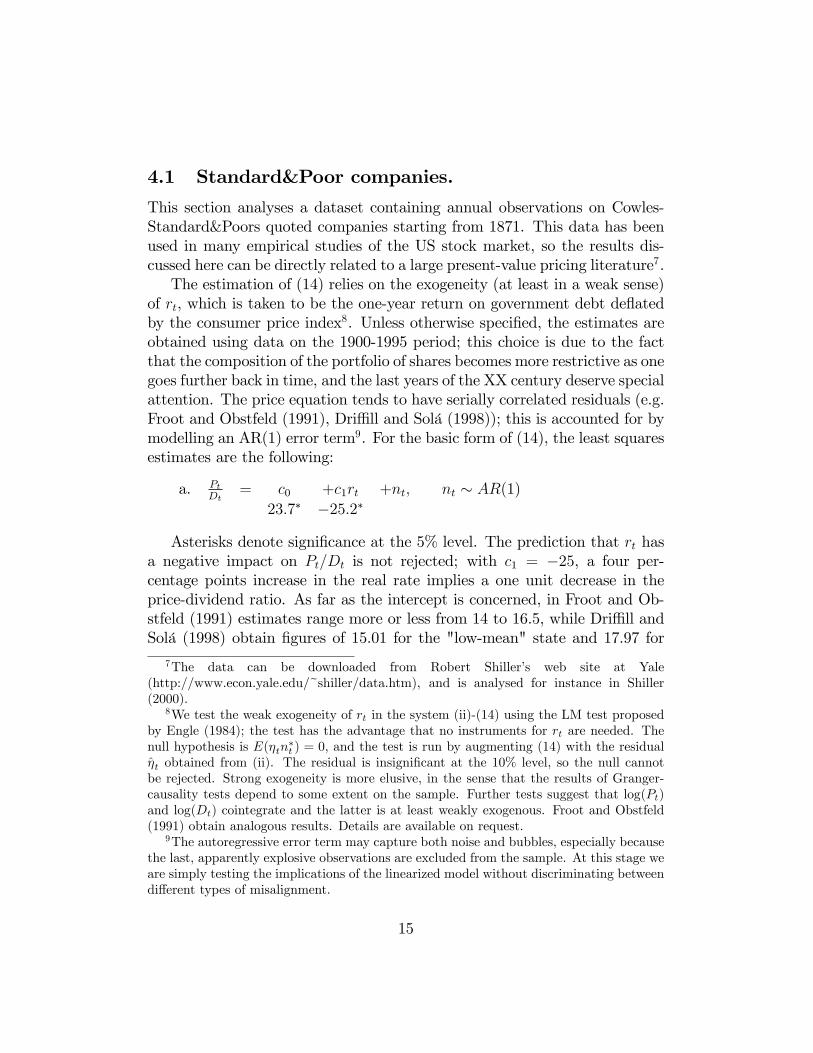
4.1 Standard&Poor companies.

This section analyses a dataset containing annual observations on Cowles-Standard&Poors quoted companies starting from 1871. This data has beenused in many empirical studies of the US stock market, so the results dis-cussed here can be directly related to a large present-value pricing literature7.The estimation of (14) relies on the exogeneity (at least in a weak sense)

of rt, which is taken to be the one-year return on government debt de�atedby the consumer price index8. Unless otherwise speci�ed, the estimates areobtained using data on the 1900-1995 period; this choice is due to the factthat the composition of the portfolio of shares becomes more restrictive as onegoes further back in time, and the last years of the XX century deserve specialattention. The price equation tends to have serially correlated residuals (e.g.Froot and Obstfeld (1991), Dri¢ ll and Solá (1998)); this is accounted for bymodelling an AR(1) error term9. For the basic form of (14), the least squaresestimates are the following:

a. PtDt

= c0 +c1rt +nt; nt � AR(1)23:7� �25:2�

Asterisks denote signi�cance at the 5% level. The prediction that rt hasa negative impact on Pt=Dt is not rejected; with c1 = �25, a four per-centage points increase in the real rate implies a one unit decrease in theprice-dividend ratio. As far as the intercept is concerned, in Froot and Ob-stfeld (1991) estimates range more or less from 14 to 16.5, while Dri¢ ll andSolá (1998) obtain �gures of 15.01 for the "low-mean" state and 17.97 for

7The data can be downloaded from Robert Shiller�s web site at Yale(http://www.econ.yale.edu/~shiller/data.htm), and is analysed for instance in Shiller(2000).

8We test the weak exogeneity of rt in the system (ii)-(14) using the LM test proposedby Engle (1984); the test has the advantage that no instruments for rt are needed. Thenull hypothesis is E(�tn

�t ) = 0, and the test is run by augmenting (14) with the residual

�t obtained from (ii). The residual is insigni�cant at the 10% level, so the null cannotbe rejected. Strong exogeneity is more elusive, in the sense that the results of Granger-causality tests depend to some extent on the sample. Further tests suggest that log(Pt)and log(Dt) cointegrate and the latter is at least weakly exogenous. Froot and Obstfeld(1991) obtain analogous results. Details are available on request.

9The autoregressive error term may capture both noise and bubbles, especially becausethe last, apparently explosive observations are excluded from the sample. At this stage weare simply testing the implications of the linearized model without discriminating betweendi¤erent types of misalignment.

15

the "high-mean" state. The estimate above is larger, probably because ofsample di¤erences. Do the restrictions make sense in terms of the underlyingdiscount factor? With � = 1:02, �0 = :02, �1 = :33 (obtained from univari-ate models for Dt and rt), the estimated ci coe¢ cients imply a � between.93 and 1.04 - an acceptable result once sample variability is taken into ac-count. If we make the further assumptions that the innovations (nt; "t; �t)are approximately normally distributed, we can estimate the trivariate sys-tem by Full-Information Maximum Likelihood and test the restrictions moreformally. Table 1 reports FIML estimates for the restricted and unrestrictedmodel. The restricted system gives � = :9410; the likelihood ratio statistic isabout .10, well below any conventional signi�cance level, so the restrictionson c0 and c1 are not rejected. Normality is of course a strong assumption,and in the case of "t and nt it can only be interpreted as an approximationto the true distribution because of the non-negativity of Pt=Dt and Dt=Dt�1.Nevertheless, the estimate of � and the extremely low value of the likelihoodratio statistic indicate that model and data are broadly consistent.

Equation (a) performs well in all the standard speci�cation tests, display-ing normal i.i.d. residuals, and it is qualitatively robust to subsampling inthe 1870-1995 period; in fact, c1 is negative and signi�cant even if the 1995-2002 years are included, but in this case the model fails most speci�cationtests. As a further check on the robustness of the estimates, we also considertwo expanded versions of the price-dividend ratio equation:

b. PtDt

= c0 +c1rt +c2�Pt�1 +c3�Dt�1 +c4Pt�1Dt�1

+nt23:7� �25:9� :0 �:0 :87�

c. PtDt

= c0 +c1rt +c1D2:61t +nt; nt � AR(1)

17:5� �22:3� :01�

Equation (b) simply includes a lag of the price, the dividend and the ratioof the two; (c) is an attempt to incorporate an "intrinsic bubble" à la Frootand Obstfeld (1991)11. Asterisks denote again signi�cance at the 5% level;

10Note that the mean one-period discount factor is E(1 + rt + �)�1 � Ef(rt), whereas� � (1 + E(rt) + �)�1 = f(E(rt)):Since f is convex, by Jensen�s inequality � � Ef(rt);in other words, the actual one-period expected discount rate is above �.11The exponent 2:61 is taken from table 3 on page 1201 of Froot and Obstfeld (1991);

results are not sensitive to this choice. We further elaborate on the intrinsic bubble modelin section 5.

16

neither the extra lags nor a power of Dt swamp the interest rate e¤ect: c1remains negative and signi�cant.The estimates are encouraging, in the sense that the assumption on the

structure of the discount factor (and the approximation) prove to have some-thing to say on the behaviour of Pt independently of the stance one takes onthe existence of speculative bubbles. In particular, the model rationalises thenegative relationship between interest rate and price-dividend ratio found inthe data, and it does it in a way which is consistent with plausible values ofthe underlying average discount factor.

The remainder of this section examines the contribution of the bubbleto the explanation of the price pattern. Some estimates for the unrestricted"reduced" model, where Pt=Dt is the measurement variable andBt the hiddenstate, are presented in table 2 and �gures 1 to 4. We report results obtainedwith two samples, 1900-1990 and 1900-2002. Again, the inclusion of the 1871-1900 period implies only marginal changes, the most interesting of which isan increase in the signi�cance of the interest rate term. This is clearly notthe case for the last decade, that stretches the model to its limits. Eachobservation after 1995 pushes the estimated average risk premium up, andthe estimate is as large as 11% when the full sample is used; for this reasonwe also report the estimates obtained imposing � = :0_612. Furthermore, theresiduals corresponding to the last observations are very large: the behaviourof the price index after 1998 is somewhat exceptional even after accountingfor a near-exponential bubble. Nevertheless, the analysis delivers some clearconclusions. The parameters of the Pt=Dt equation, including the interestrate term, are signi�cant, rightly signed and of a reasonable magnitude. Thepattern of the bubble is realistic: it remains latent during the �rst 50 years (infact, it is also insigni�cantly di¤erent from zero throughout the XIX century),and it drives prices up in the 60�s and in the second half of the 90�s13. For

12As LeRoy (2004) stresses, the existence of rational bubbles cannot explain the equitypremium puzzle of Mehra and Prescott (1985). The excess return on equity has beenvery high in the past decades, and this is puzzling independenly of whether the price levelcontained a bubble or not. Note also that as long as � > 0 the bubble is explosive and �has a non-standard distribution; the signi�cance levels reported in table 2 are valid insofaras this is approximately normal.13There is an issue with the sign of the price bubble. Negative bubbles are usually

ruled out because they imply a non-zero probability of prices becoming negative in thefuture. However, temporary undervaluation due to a short-lived negative bubble appearsto be a realistic possibility (Wu (1997)). Our estimation procedure does not impose a

17

these two periods, and notably for the second one, the estimated bubble issigni�cant well above the 5% level independently of whether the risk premiumis restricted or not14. It is interesting to compare the results to Wu (1997),where the bubble is estimated by Kalman-�ltering under the assumption of aconstant discount factor. The bubble estimated by Wu follows a remarkablysimilar path, and between 1960 and 1970 it accounts on average for 40-50%of the price level; our estimates suggest a �gure of 30-40% (more details aregiven in table 5). The type of time-variation in the discount factor assumedin this model reduces the estimated size of the bubble by roughly 10%.As a further robustness test, the model was also estimated expanding

the measurement equation to include alternatively a lagged price-dividendratio and an "intrinsic bubble" (again with a constant exponent). The extraterms are generally signi�cant and the lagged price-dividend ratio reducesthe size of the bubble; however, Bt remains highly signi�cant in both casesand follows a very similar path. Besides, the lagged price-dividend ratio iscompletely ad hoc and its presence in the equation is even more di¢ cult tojustify than that of the bubble itself. The residuals do not display any clearpattern. Though, the diagnostics in table 2 show that the last observationsweaken the evidence that the "noise" is an i.i.d. normal variable; this ispartially due to the model�s inability to anticipate the burst of the bubble,which generates inaccurate forecasts for 2001 and 2002.

What to make of this result? We already noted that there is a long andarticulated debate on the theoretical and empirical plausibility of rationalbubbles. A few recent empirical works provided ground for scepticism byshowing that fundamentals can explain a lot depending on how they aremeasured and modelled. Wright (2004) adjusts the dividend series by nettingout new issues and buybacks and shows that the adjusted dividend yieldbehaves more regularly, displaying no negative drift in the last decade ofthe century. Using ordinary S&P data and assuming constant discounting,Dri¢ ll and Solá (1998) show that a dividend process switching between a"bad" state (low mean-high variance) and a "good" state (high mean-lowvariance) also goes a long way towards explaining movements in the price

non-negativity constraint on the bubble process.14The error bands shown in the �gures 2 and 4 quantify the "�lter uncertainty" ignoring

the "parameter uncertainty" (Hamilton (1994)); since the system is very parsimoniousand the parameters are estimated with good accuracy, this is unlikely to be a seriousshortcoming.

18

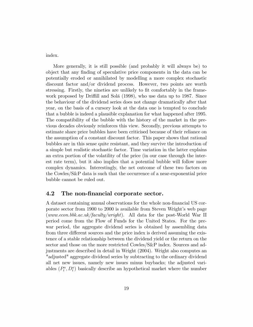
index.

More generally, it is still possible (and probably it will always be) toobject that any �nding of speculative price components in the data can bepotentially eroded or annihilated by modelling a more complex stochasticdiscount factor and/or dividend process. However, two points are worthstressing. Firstly, the nineties are unlikely to �t comfortably in the frame-work proposed by Dri¢ ll and Solá (1998), who use data up to 1987. Sincethe behaviour of the dividend series does not change dramatically after thatyear, on the basis of a cursory look at the data one is tempted to concludethat a bubble is indeed a plausible explanation for what happened after 1995.The compatibility of the bubble with the history of the market in the pre-vious decades obviously reinforces this view. Secondly, previous attempts toestimate share price bubbles have been criticised because of their reliance onthe assumption of a constant discount factor. This paper shows that rationalbubbles are in this sense quite resistant, and they survive the introduction ofa simple but realistic stochastic factor. Time variation in the latter explainsan extra portion of the volatility of the price (in our case through the inter-est rate term), but it also implies that a potential bubble will follow morecomplex dynamics. Interestingly, the net outcome of these two factors onthe Cowles/S&P data is such that the occurrence of a near-exponential pricebubble cannot be ruled out.

4.2 The non-�nancial corporate sector.

A dataset containing annual observations for the whole non-�nancial US cor-porate sector from 1900 to 2000 is available from Steven Wright�s web page(www.econ.bbk.ac.uk/faculty/wright). All data for the post-World War IIperiod come from the Flow of Funds for the United States. For the pre-war period, the aggregate dividend series is obtained by assembling datafrom three di¤erent sources and the price index is derived assuming the exis-tence of a stable relationship between the dividend yield or the return on thesector and those on the more restricted Cowles/S&P index. Sources and ad-justments are described in detail in Wright (2004). Wright also computes an"adjusted" aggregate dividend series by subtracting to the ordinary dividendall net new issues, namely new issues minus buybacks; the adjusted vari-ables (P at ; D

at ) basically describe an hypothetical market where the number

19

of shares remains constant at the 1900 level15.

Figure 5 plots the price-dividend ratio for S&P companies together withthe ordinary and adjusted ratios for the whole non-�nancial sector. Clearly,both the expansion of the set of companies and the adjustment for net newissues have a signi�cant impact on the variable. The pattern of the non-adjusted sector ratio is qualitatively similar to the S&P benchmark; themain di¤erence is that the peak in the late nineties is much smaller, leavingless room for rational bubbles. As Robertson and Wright (2003) and Wright(2004) document, the consequences of adjusting for issues and buybacks aredramatic. The adjusted ratio has no clear upward trend in the second halfof the sample, and it displays "fat tailed volatility"; in particular, two largespikes in the late twenties and early seventies (in coincidence with largenet equity issues) complicate the statistical modelling of the variable. Theadjusted ratio is the only one for which the null hypothesis of a unit root iscon�dently rejected by the standard augmented Dickey-Fuller tests.

Preliminary analyses involve checking the adequacy of (i) and the weakexogeneity of rt in the price-dividend ratio equation16. Figure 6 shows thegrowth rates of ordinary and adjusted dividends (Dt=Dt�1, Da

t =Dat�1). A

regression of Dt=Dt�1 on a constant delivers serially uncorrelated residualsand an estimated dividend growth rate of about 3%. The growth rate of theadjusted dividend is more volatile and it peaks above 100% three times overthe sample. In this case, a simple regression of the growth rate on a con-stant generates serially correlated and heteroscedastic residuals. The corre-lation is signi�cantly mitigated if the extreme observations are ignored or theinnovation is modelled as conditionally heteroscedastic (via an ARCH(1)).

15Robertson and Wright (2003) and Wright (2004) argue that this "broad dividend"is theoretically more appropriate than the usual, "narrow" dividend. Others (e.g. Coleet al. (1996)) express doubts on the equivalence between dividends and repurchases.According to LeRoy (2004), the two variables simply describe di¤erent porfolio strategies,either of which may have a bubble or not. But arguably a representative agent holdinga representative share can only implement one such strategy, and this is linked to the"broad" dividend measure.16In what follows, the safe rate rt is again the nominal return on one-year public debt

de�ated by the Consumer Price Index, available from Shiller. As long as the dependentvariable is the price-dividend ratio, any de�ator can potentially be used to obtain the realinterest rate.

20

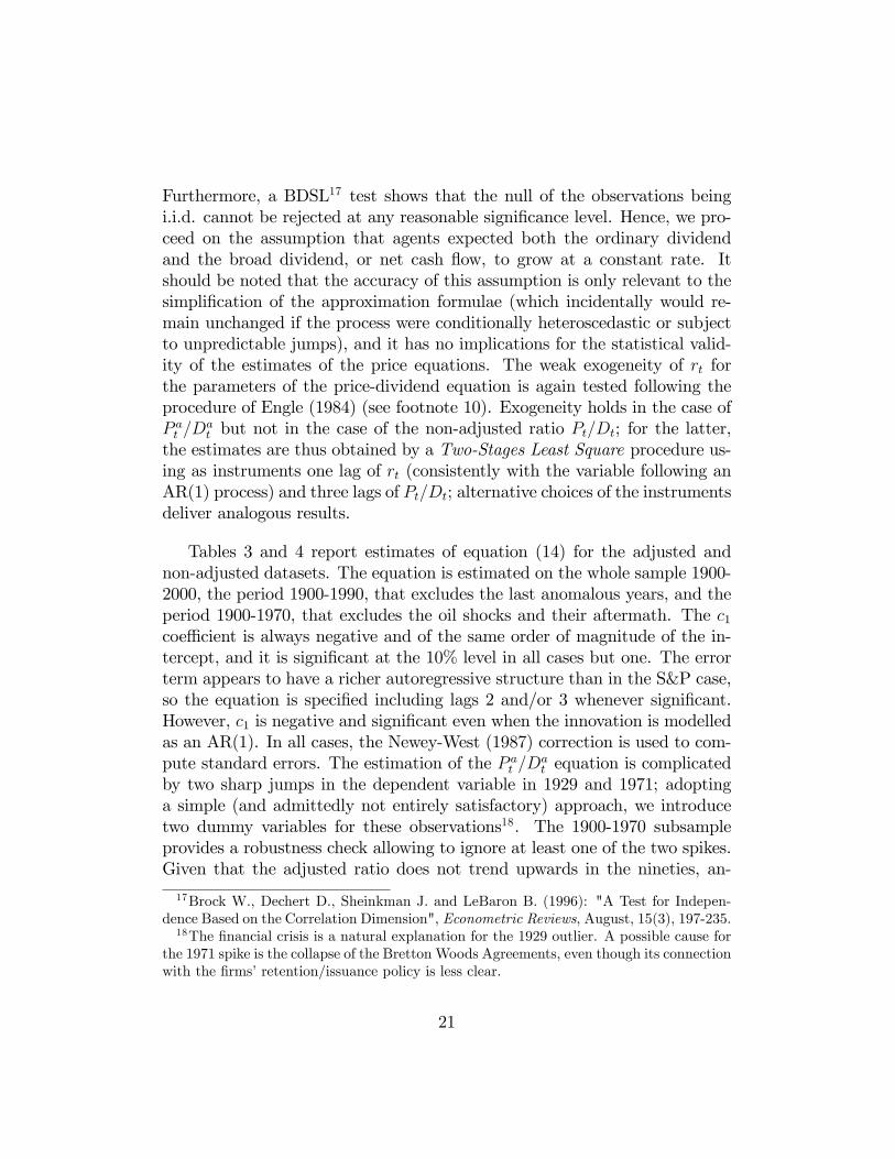
Furthermore, a BDSL17 test shows that the null of the observations beingi.i.d. cannot be rejected at any reasonable signi�cance level. Hence, we pro-ceed on the assumption that agents expected both the ordinary dividendand the broad dividend, or net cash �ow, to grow at a constant rate. Itshould be noted that the accuracy of this assumption is only relevant to thesimpli�cation of the approximation formulae (which incidentally would re-main unchanged if the process were conditionally heteroscedastic or subjectto unpredictable jumps), and it has no implications for the statistical valid-ity of the estimates of the price equations. The weak exogeneity of rt forthe parameters of the price-dividend equation is again tested following theprocedure of Engle (1984) (see footnote 10). Exogeneity holds in the case ofP at =D

at but not in the case of the non-adjusted ratio Pt=Dt; for the latter,

the estimates are thus obtained by a Two-Stages Least Square procedure us-ing as instruments one lag of rt (consistently with the variable following anAR(1) process) and three lags of Pt=Dt; alternative choices of the instrumentsdeliver analogous results.

Tables 3 and 4 report estimates of equation (14) for the adjusted andnon-adjusted datasets. The equation is estimated on the whole sample 1900-2000, the period 1900-1990, that excludes the last anomalous years, and theperiod 1900-1970, that excludes the oil shocks and their aftermath. The c1coe¢ cient is always negative and of the same order of magnitude of the in-tercept, and it is signi�cant at the 10% level in all cases but one. The errorterm appears to have a richer autoregressive structure than in the S&P case,so the equation is speci�ed including lags 2 and/or 3 whenever signi�cant.However, c1 is negative and signi�cant even when the innovation is modelledas an AR(1). In all cases, the Newey-West (1987) correction is used to com-pute standard errors. The estimation of the P at =D

at equation is complicated

by two sharp jumps in the dependent variable in 1929 and 1971; adoptinga simple (and admittedly not entirely satisfactory) approach, we introducetwo dummy variables for these observations18. The 1900-1970 subsampleprovides a robustness check allowing to ignore at least one of the two spikes.Given that the adjusted ratio does not trend upwards in the nineties, an-

17Brock W., Dechert D., Sheinkman J. and LeBaron B. (1996): "A Test for Indepen-dence Based on the Correlation Dimension", Econometric Reviews, August, 15(3), 197-235.18The �nancial crisis is a natural explanation for the 1929 outlier. A possible cause for

the 1971 spike is the collapse of the Bretton Woods Agreements, even though its connectionwith the �rms�retention/issuance policy is less clear.

21

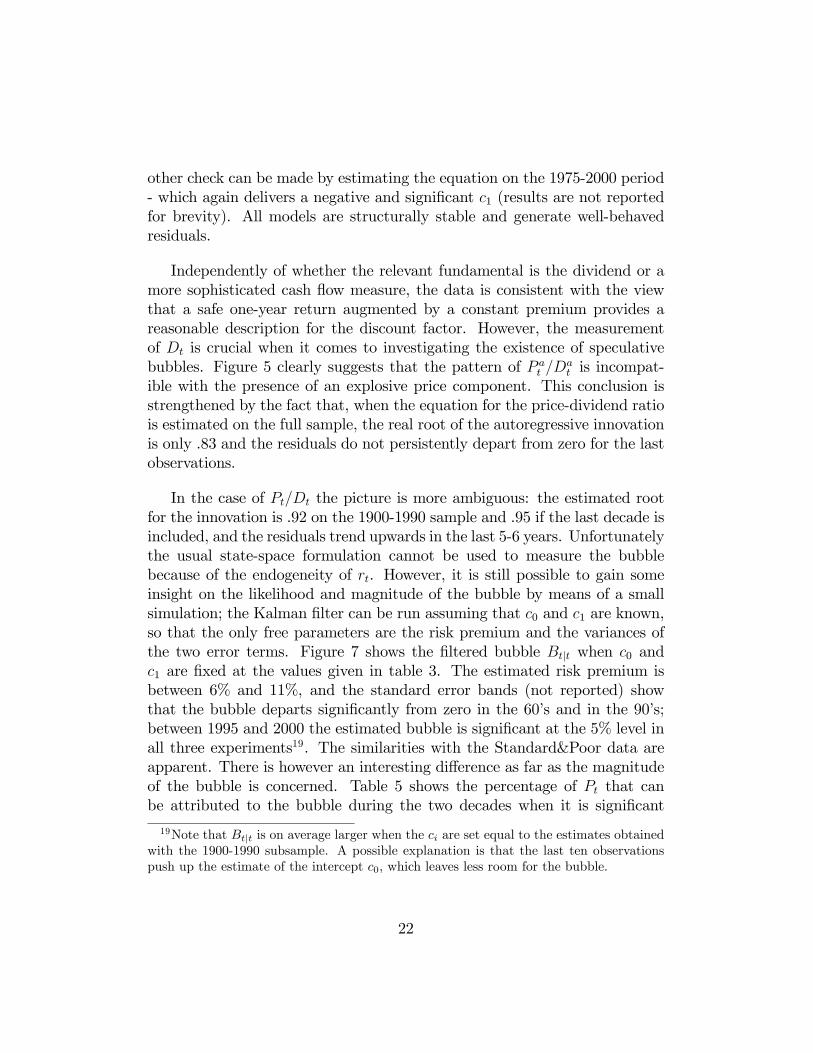
other check can be made by estimating the equation on the 1975-2000 period- which again delivers a negative and signi�cant c1 (results are not reportedfor brevity). All models are structurally stable and generate well-behavedresiduals.

Independently of whether the relevant fundamental is the dividend or amore sophisticated cash �ow measure, the data is consistent with the viewthat a safe one-year return augmented by a constant premium provides areasonable description for the discount factor. However, the measurementof Dt is crucial when it comes to investigating the existence of speculativebubbles. Figure 5 clearly suggests that the pattern of P at =D

at is incompat-

ible with the presence of an explosive price component. This conclusion isstrengthened by the fact that, when the equation for the price-dividend ratiois estimated on the full sample, the real root of the autoregressive innovationis only .83 and the residuals do not persistently depart from zero for the lastobservations.

In the case of Pt=Dt the picture is more ambiguous: the estimated rootfor the innovation is .92 on the 1900-1990 sample and .95 if the last decade isincluded, and the residuals trend upwards in the last 5-6 years. Unfortunatelythe usual state-space formulation cannot be used to measure the bubblebecause of the endogeneity of rt. However, it is still possible to gain someinsight on the likelihood and magnitude of the bubble by means of a smallsimulation; the Kalman �lter can be run assuming that c0 and c1 are known,so that the only free parameters are the risk premium and the variances ofthe two error terms. Figure 7 shows the �ltered bubble Btjt when c0 andc1 are �xed at the values given in table 3. The estimated risk premium isbetween 6% and 11%, and the standard error bands (not reported) showthat the bubble departs signi�cantly from zero in the 60�s and in the 90�s;between 1995 and 2000 the estimated bubble is signi�cant at the 5% level inall three experiments19. The similarities with the Standard&Poor data areapparent. There is however an interesting di¤erence as far as the magnitudeof the bubble is concerned. Table 5 shows the percentage of Pt that canbe attributed to the bubble during the two decades when it is signi�cant

19Note that Btjt is on average larger when the ci are set equal to the estimates obtainedwith the 1900-1990 subsample. A possible explanation is that the last ten observationspush up the estimate of the intercept c0, which leaves less room for the bubble.

22

at the 5% level in both the S&P and the non-�nancial sector data20. Bothprices in�ate by an average 30-40% during the �rst surge of the bubble.The situation is di¤erent in the nineties: the price of a non-�nancial shareincreases by about 20% with a peak of 50% in 2000, whereas for an S&Pshare the average price increase is around 40% and the 2000 maximum is+73%. These �gures are obviously subject to some margin of error. However,this is likely to be roughly of the same size in the two datasets, and it ispresumably unrelated to the sample period. Hence, such a large discrepancyin the estimates is a reliable indicator of a substantial divergence betweenthe true underlying bubble processes.

As long as we stick with the traditional de�nition of dividends, it seemshard to exclude that an exponential speculative bubble may have pushedshare prices up at least twice in the last century, and most notably in the90�s. At the same time, though, the dimensions of the presumed bubbledepend quite substantially on how broad is the set of �rms considered. In away, even a "broad market index" like S&P500 is not entirely representativeof the whole non-�nancial US sector: overvaluation is quantitatively lessimportant when looking at industry-level data.

If one accepts the idea that the Miller-Modigliani theorem has to be takenmore seriously, and that net share repurchases are equivalent to dividends,the picture changes substantially. In this case, a more technical analysis con-�rms what a qualitative assessment of the data already suggests - namelythat the bubble does not exist. Since there is again evidence of time-varyingdiscounting of the type discussed in the previous sections, the approximationstill gives some guidance in investigating price dynamics; in particular, itprovides a more articulated de�nition of "fundamental price" than that im-plied by constant discount models. The di¤erence is that, on adjusted data,the deviations of actual prices from this benchmark �t better the concept ofshort-lived fads or generic noise than that of a proper speculative bubble.

20The bubble for the non-�nancial sector is �ltered �xing c0 and c1 at 26:1 and �39:3;namely their estimates on the 1900-1990 sample. These values are preferable because theyexclude the obviously bubbly years 1990-2000 (so that, for instance, c0 is very close tothe sample mean of Pt=Dt) without any further, unnecessary shortening of the sample.As noted above, this is likely to give an upper bound for the actual bubble. Again, thesigni�cance level is computed disregarding any uncertainty stemming from the estimatedparameters.

23

5 Intrinsic or extrinsic?

Among the bubble-based explanations of the behaviour of the American stockmarket in post-war years, one that has received signi�cant attention is thealready mentioned intrinsic bubble studied by Froot and Obstfeld (1991).They de�ne bubbles as "intrinsic" when "they derive all of their variabilityfrom exogenous economic fundamentals and not from extraneous factors"(page 1). Note that according to this de�nition the bubble examined in theprevious section does not qualify as intrinsic: it depends on fundamentalsbecause the rate of growth is a function of rt, but, due to the presence ofthe bt shocks, it also introduces an extraneous source of variability in theprice process. Froot and Obstfeld derive a simple parametrisation by whichthe bubble is a power of the dividend itself. They examine the 1900-1988period using Standard&Poors dividend and price series, and show that thenon-linearity of the price-dividend relation is not rejected by the data. Theobjective of this section is to replicate the analysis of Froot and Obstfeld(1991) on a more comprehensive set of data: how does the intrinsic bubblefare in the 90�s? And what happens when the whole non-�nancial industryis considered, or the dividend series is adjusted by netting out issues andbuybacks? The purpose of this exercise is not only to compare the per-formance of two di¤erent formulations of the bubble process, but also - andmore importantly- to �nd out whether the intrinsic bubble can be considereda candidate to explain the failure of the Q model of investment.

Froot and Obstfeld (1991) consider the case where the instantaneous rateof interest is constant (r) and the log dividend follows a random walk: dt+1 =�+dt+�t+1; with �t+1jt � N(0; �2). The focus is thus on the following period-by-period equation: Pt = e�rEt(Pt+1 + Dt). The authors show that, if notransversality condition is imposed, the price equation has a forward solutionof the type Pt = kDt + cD

�t , where k � (er � e�+�2=2)�1, c is an arbitrary

constant and � is the positive root of �2�2=2 + �� � r = 0. An attractivefeature of this approach, not shared by the exponential bubble, is that it canexplain the high sensitivity of prices to �rms�dividend announcements. Theempirical analysis focusses on equation (13), page 1198:

PtDt

= c0 + cD��1 + �t;

where the error term �t is by assumption independent of dividends at all leadsand lags. Note that, since this equation is derived under the assumption that

24

the discount rate is constant, a direct comparison between the two bubblespeci�cations (intrinsic and exponential) is not straightforward. In otherwords, an equation like (b) on page 12, that contains both rt and D��1

t ,cannot be given a rigorous theoretical interpretation.

As Froot and Obstfeld point out, a random walk can be considered at bestan approximation to the true process agents use to forecast dividends. Inparticular, stock prices, which re�ect a broad (possibly the broadest) infor-mation set available at each point in time, may well contain information onfuture dividends beyond that given by the current dividend. Obviously thisalso applies to the discussion in the previous sections - the BDSL test simplyshows that an agent expecting the dividend to grow at a constant rate did notcommit gross, systematic mistakes over the sample period. When it comesto estimating the equation above, though, the issue becomes critical in tworespects. Firstly, consistent estimation of c by OLS requires Et(�tjDt) = 0.Secondly, Froot and Obstfeld conduct inference on c relying on the assump-tion that �t is independently distributed of �t at all leads and lags: appendixB of their paper shows that in this case the t statistic for the null hypothesiscOLS = 0 is asymptotically normal despite the explosive regressor. In thenon-�nancial industry data (both adjusted and non-adjusted) there is evi-dence of Granger-causality running from prices to dividends; independencebetween �t and �s for all t and s is admittedly a strong assumption, and itdoes not fare too well on these series. Fortunately, it is possible to extendFroot and Obstfeld�s discussion to show that a 2SLS procedure where Dt isinstrumented by its own lag preserves both consistency of c and asymptoticnormality of the t statistic under the less stringent assumption that �t isindependent of past dividend innovations �s (s = 1; :::; t� 1).

Table 6 expands the available evidence on the american intrinsic bubble.For each of the three datasets (S&P, non-�nancial industry, adjusted non-�nancial industry) the price-dividend ratio equation is estimated with andwithout the 1990-2000 observations21. For the S&P data we report OLS

21All equations allow for an AR(1) error term, as in rows 2 and 4 of table 3 of the originalpaper, and are estimated imposing the value of � implied by the estimates of �2, � andr. Depending on the dataset and the sample period, � goes from a minimum of 1.33 toa maximum of 2.81; Froot and Obstfeld compute � = 2:74. Sensitivity analysis con�rmsthat the results are qualitatively robust to the value of �: If this is estimated concurrentlywith the other parameters by a non-linear least squares procedure, the estimates are of asimilar magnitude (as in Froot and Obstfeld), but the standard errors tend to be large.

25

estimates: 2SLS estimates are very similar, which is consistent with bothFroot and Obstfeld�s assessment of the exogeneity of the dividend and ourown; for the other two datasets we report 2SLS.

The �rst row of table 6 is basically a replica of Froot and Obstfeld�s result:with a positive and signi�cant c, prices become increasingly overvalued asdividends rise, consistently with the model�s prediction22. The fourth rowshows that the model fails to explain the behaviour of the S&P price indexin the 90�s: when the 1990-2000 observations are considered, the intrinsicbubble looses its signi�cance and the estimated root of the autoregressiveerror jumps well above unity. If the 90�s are to be explained by assuming theexistence of an explosive price component, an exponential process appears tobe a better choice than a power of the dividend.Rows two and �ve test the intrinsic bubble hypothesis using non-adjusted

data for the whole non-�nancial sector. On pre-1990 data, the c coe¢ cientis correctly (i.e. positively) signed and signi�cantly di¤erent from zero atthe 10% level, but it is estimated with a relatively large standard error.Interestingly, the signi�cance of the bubble increases when the full sampleis used. Furthermore, the unexplained serial correlation appears in this caseto be stationary. The estimate c = 4:79 is not entirely convincing, in thesense that it implies a surprisingly high degree of "sensitivity" of the price tothe contemporaneous dividend, but the theory places no restriction on themagnitude of this coe¢ cient. Finally, results for the adjusted series (rowsfour and six) leave little room for ambiguity: c is far from any acceptablesigni�cance level in both samples, and wrongly signed in one of them.

The adjustment for new issues and buybacks is as lethal for the intrinsicbubble as it is for the exponential bubble; again, this is hardly surprisinggiven the strong mean-reversion displayed by the adjusted price-dividend ra-tio. As far as the non-adjusted data is concerned, it seems fair to say thaton the whole the intrinsic bubble performs worse than the exponential bub-ble studied in the previous sections. The two formulations are both broadlycompatible with price patterns between 1900 and 1990, but the following tenyears provide a clear case for the exponential bubble. The growth of the

22Froot and Obstfeld note that the equation "does a better job" on post-war data(p.1204). Indeed, a formal Chow test rejects the null hypothesis of structural stabilitybefore and after 1945 at the 1% con�dence level. However, magnitude and signi�cance ofc are more or less unchanged when the pre-war period is ignored.

26

non-�nancial industry share price can be explained within Froot and Obst-feld�s (1991) framework, even though this comes at the cost of a somewhatimplausibly strong link between price and contemporaneous dividend. Butthe rise in the S&P index is simply too large and sudden to be justi�ed bythis type of mechanism.

These �ndings cast some doubts on the overall plausibility of the intrinsicbubble story. One would expect that, if there is a bubble of any type in theindustry-level data, this will also appear in market indices based on a largeset of �rms, such as Standard&Poor�s. This is the case for the exponentialbubble, but not for the intrinsic one. Furthermore, the bubble modelled byFroot and Obstfeld is a deterministic function of the dividend and, as such,it cannot pop and re-start at di¤erent points in time: the lack of signi�canceof the intrinsic bubble in a period of widely aknowledged price misalignmentis in this sense particularly di¢ cult to justify. Of course one may argue thatprices contain both a permanent intrinsic bubble and occasional, stochasticexponential bubbles, and that the latter swamp the former during their ex-pansion phases. Albeit theoretically admissible, this possibility strikes us asunrealistic.

6 Conclusion

Economists have been puzzled by stock markets for a long time, and recentexperiences in the US and elsewhere have revived debates dating back atleast to the eighties: how much can fundamentals explain? Are prices really"too volatile"? Price misalignments, and rational bubbles in particular, area fascinating hypothesis, but one on which there is no consensus on eithertheoretical or empirical grounds. In this paper we discuss a state-space modelthat allows maximum likelihood estimation of share price bubbles conditionalon di¤erent assumptions on the stochastic discount factor. The bubbles arealso stochastic, and they grow at a time-varying rate given by the inverse ofthe one-period discount factor. The model is used to analyse three long seriesof annual observations on the US, namely a Standard&Poors dataset, a non-�nancial industry dataset, and an adjusted non-�nancial industry datasetwhere the dividend is computed netting out new share issues and buybacks.We assume that investors discount expected dividends on the basis of a safeone-year return augmented by a constant risk premium.

27

This assumption �ts the data reasonably well: the price-dividend ratiois negatively correlated to the contemporaneous real interest rate, and themagnitude of this e¤ect is consistent with the interpretation we propose.As far as misalignments are concerned, our estimates sketch the followingpicture. The S&P price index was in�ated by rational bubbles twice in thelast century, in the sixties and in the nineties. This is also true for the priceof a non-�nancial company share, though the bubble of the nineties wasproportionally much smaller. Finally, there are no bubbles in the adjustedshare price; variation in the interest rate does not completely explain pricedynamics in this case either, but what is left resembles short-lived fads ratherthan a bubble. Our work suggests two conclusions that should be of someinterest independently of the position one takes on the existence of rationalbubbles. The �rst one is that self-ful�lling bubbles and stochastic discountingmay coexist; in particular, bubbles are a possible explanation for the excessvolatility of prices over dividends and interest rates already documented inthe literature. The second one is that investigations of this type are verysensitive to the way variables are de�ned; for a shareholder looking not justat dividends but also at share issues and repurchases, the nineties were aperfectly ordinary decade.

7 Appendix

7.1 Derivation of equation (3)

This appendix illustrates the derivation of the Taylor expansion. We stressagain that this is merely a bivariate extension of an approximation originallyused in Poterba and Summers (1986). De�ne the sequences frtg � rt; rt+1; :::and f�tg � �t; �t+1; ::: and consider the following function23:

f(frtg ; f�tg) �1Xi=0

iYj=0

(1 + rt+j + �t+j)�1

!Dt+i (A1)

A �rst-order Taylor approximation of f in a neighborhood of (�r; ��) �E(rt; �t) has the following form:

23We follow Poterba and Summers (1986) in letting the summation start in i = 0; theimplicit timing convention is that the contemporaneous dividend accrues to the time-tbuyer of the share.

28

f(frg ; f�g) ' f(�r; ��) +

+

"@f

@ frtg

����(�r;��)

#(frtg � �r)

+

"@f

@ f�tg

����(�r;��)

#(f�tg � ��): (A2)

The computation of the �rst term is straightforward:

~PLt � f(_r;_�) =

1Xi=0

�1

1 +_r +

_�

�i+1Dt+i �

1Xi=0

�i+1Dt+i (A3)

where � � (1 +_r +

_�)�1: Because rt+j and �t+j enter f in the same way,

the partial derivatives of f with respect to these variables have the samefunctional form. To derive it, note �rst that:

@f

@rt+i= �(1 + rt+i + �t+i)�1

1Xk=0

i+kYj=0

(1 + rt+j + �t+j)�1

!Dt+i+k

Consequently:

@f

@rt+i

����(_r ;_�)

= ��i+11Xk=0

�k+1Dt+i+k

"@f

@rt+i

����(_r ;_�)

#(rt+i � �r) =

"��i+1

1Xk=0

�k+1Dt+i+k

#(rt+i � �r)

The �rst-order Taylor term for frtg is given by the summation over i ofthe equations above:

~Rt �"@f

@ frtg

����(_r ;_�)

#(frtg �

_r)

=

1Xi=0

("��i+1

1Xk=0

�k+1Dt+i+k

#(rt+i �

_r)

)(A4)

29

An analogous formula can be derived for ~At; the term involving the riskpremium. By the linearity of the expectation operator we can write:

P ft = Et [f(frtg ; f�tg)] ' Eth~PLt +

~Rt + ~At

i= Et ~P

Lt + Et

~Rt + Et ~At (A5)

Hence, the only condition needed to derive (A5) is the existence of a�nite unconditional mean for rt and �t. If Et ~PLt , Et ~Rt and Et ~At are equalto PLt ; Rt and At as de�ned in (4), (5), and (6), we then obtain a bivariateversion of equation (4) of Poterba and Summers (1986). This requires furtherassumptions on the processes generating dividends, interest rates and riskpremia.

A su¢ cient condition for Et ~PLt = PLt is the absolute summability of the

series:P1

i=1Et���iDt+i

�� < 1: This condition holds (or is assumed to hold)for most common speci�cations of the dividend process. In the case of theother two variables on the right hand side of (A5) the derivation is morecumbersome, even though it does not require sophisticated mathematics. Ageneral discussion is beyond the scope of the paper; we brie�y comment onthe relationship between Et ~Rt and Rt in the following case:Dt = �Dt�1 + "t; "t � N(0; �2");rt = �0 + �1rt�1 + �t; �t � N(0; �2�); j�1j < 1;8t : E("t�t) = ���;8t 6= s : E("t"s) = E(�t�s) = E("t�s) = 0:If �"� = 0, we obtain Et ~Rt = Rt. If �"� 6= 0, Et ~Rt also contains a

covariance term; it is possible to show that this is bounded by a multiple of�"� itself, so it is �nite (despite the in�nite summation over i and k) and itis "small" for "small" values of the contemporaneous covariance between theinnovations in Dt and rt. On the three datasets used in the paper, bivariatesystems for the growth rate of the dividend and the real interest rate deliver�"� ' :003. Finally, as long as �"� is constant, ignoring the covariance termin Rt can at worst complicate the interpretation of the intercept of the priceequation but it has no impact on the dynamics. Since there is no evidenceof a time-varying conditional covariance, the result is quite reassuring. Ofcourse this point may become more delicate when modelling higher frequencydata. The equality Et ~At = At can be derived along the same lines insofaras the underlying process for the risk premium �t has suitable properties.Details on the derivation are available upon request.

30

7.2 Caveats on the state-space formulation

This section highlights some issues that should be taken into account whenconsidering further speci�cations and applications of the general state-spacemodel used in the paper. Chen et al. (2001) provides a good starting pointto clarify the risks connected to "assuming away" variation in one of thecomponents of the discount factor. Let us de�ne xt � �t+ rt and collect theterms with the same index i in (3):

P ft '1Xi=1

EtDt+i

(1 +_x)i

+

1Xi=1

@P ft@xt+i

(Etxt+i �_x):

The authors assume rt = r and (�t+1 �_�) = �(�t �

_�) + "t+1 , where

� � E(�t). What happens with a time-varying interest rate? Considerthe simple case where (i) (rt+1 �

_r) = �1(rt �

_r) + �t+1, (ii) �1 = � and

(iii) E(�t"s) = 0 8t; s. Then xt is itself an AR(1) process with root equalto � and the state-space formulation of Chen et al. (2001) is statisticallycorrect, even though interpreting the estimation results is di¢ cult becausethe �ltered state is xt and not �t as the authors claim. But these assumptionsare arbitrary: rt and �t need not be AR(1) processes; even if they are, thereis clearly no reason why they should have identical roots. Risk premium andriskless return have to be modelled separately, and ideally the state-spacesystem should include an equation for each of them.

If a simplifying assumption is to be introduced, a constant premium seemsto be better than a constant interest rate. One obvious reason is that whenthe empirical analysis is based on long low-frequency data a constant safe re-turn is clearly counterfactual: we do not know if and how �t changed duringthe last century, but we know for sure that rt moved continuously. Further-more, rt typically displays a strong autoregressive pattern (this need not bethe case for the risk premium), and ignoring it amounts to passing it to theresiduals. Finally, devicing an equation for �t is not a trivial task. Two routesare available in the context of the state-space system. The �rst one, followedby Chen et al. (2001), is to treat the premium as a further non-observablestate variable and simply postulate its process. This allows maximum likeli-hood estimation of the pattern of �t. However, since it is di¢ cult to justifythe choice of any particular process for �t on theoretical grounds, we end upappending to the model an arbitrary component. Furthermore, the estima-tion becomes technically more problematic: in this scenario the Bt equation

31

contains a product between non-observables, so the model can only be esti-mated using an approximate �ltering procedure that relies on a �rst-orderTaylor expansion of the transition equation (Harvey (1989)). Since the mea-surement equation is itself the outcome of a linearization, this is clearly notdesirable. In Chen et al. (2001) this problem is avoided by assuming thatthe bubble grows at a constant rate (1 + r + �), but this is inconsistent: aprice bubble cannot grow at a constant rate in a world were the discountfactor changes over time.

The alternative is to link the premium to some observable variable andidentify its generating process in the data. For instance, Poterba and Sum-mers (1986) use the linear relationship between equity premium and varianceof equity returns derived by Merton (1973); they model �t as an AR(1) be-cause in their daily dataset the variance is well described by this type ofprocess. On annual data, the variance of market returns does not displayclear autoregressive dynamics; if Merton�s (1973) equation is to be used, itis necessary to think of more sophisticated processes. An interesting possi-bility is to model the premium as a regime-switching variable. If �t has alow-mean and a high-mean state, At has to be computed taking into accountthe possibility of �t moving between the two in the future. The occurrenceof isolated, short periods of high volatility in the stock market may then helpexplain high equity prices over long horizons. The implementation of thisidea is left for future research.

The dynamics of At and Rt also deserve a comment. Chen et al. (2001)show that At follows by construction a process of this type:

At+1 = ��1At + P

Lt (Et�t+1 �

_�) + �t+1;

�t+1 � �1Xi=1

�i1Xk=0

�k+1Et+1Dt+1+i+k(Et+1�t+1+i �_�)

+1Xi=2

�i�11Xk=0

�k+1EtDt+i+k(Et�t+i �_�):

This can be derived by simply substituting the de�nition of At and At+1 in(At+1 � ��1At) and rearranging the terms in an appropriate fashion. With

32

the bivariate approximation, an analogous equation also holds for Rt+1 once�t is replaced with rt. The estimation procedure the authors follow relies onthe claim that Et�t+1 = 0 by the law of iterated expectations, and implicitlyassumes that �t is serially uncorrelated. For the case where Dt grows ata constant expected rate and �t � AR(1), �t can be derived analyticallyand it turns out that E(�t�t�1) 6= 0 unless further assumptions are madeon the innovations of these two processes. It is thus preferable to model theconditional expectation of Dt+i+k, �t+i and rt+i explicitly and use (5) and (6)to place restrictions on the price-dividend ratio equation. This strategy mayobviously be unattractive (or unfeasible) if Dt, �t and rt follow particularlycomplicated processes.

References

[1] Abel A.B., Blanchard O.J. (1986) - The present value of pro�ts andcyclical movements in investment, Econometrica 54(2), 249-273.

[2] Abreu D., Brunnermeier M.K. (2003) - Bubbles and crashes, Economet-rica, 71, 173-204.

[3] Black F. (1986) - Noise, Journal of Finance, 41, 529-543.

[4] Blanchard O., Rhee C., Summers L. (1993) - The stock market, pro�tand investment, Quarterly Journal of Economics, 108(1), 115-136.

[5] Blanchard O., Watson M. (1982) - Bubbles, rational expectations and�nancial markets, in P. Wachtel editor "Crisis in the economic and �-nancial structure", Lexington Books.

[6] Bond S.R., Cummins J.G. (2001) - Noisy share prices and the Q modelof investment, Institute for Fiscal Studies Working Paper 01/22.

[7] Burmeister E., Wall K. (1982) - Kalman �ltering estimation of unob-served rational expectations with an application to the German hyper-in�ation, Journal of Econometrics, 20, 255-284.

[8] Campbell J.Y., Lo A.W., MacKinlay A.C. (1997) - The econometrics of�nancial markets, Princeton University Press.

33

[9] Campbell J.Y., Shiller R.J. (1988) - The dividend-price ratio and the ex-pectations of future dividends and discount factors, Review of FinancialStudies, 1(3), 195-228.

[10] Chen L.T., Hueng C.J., Lin C.J. (2001) - Do bubbles and time-varyingrisk premiums a¤ect stock prices? A Kalman �lter approach, Universityof Alabama, working paper n. 00-04-02.

[11] Cole K., Helwege J., Laster D. (1996) - Stock market valuation indica-tors: is this time di¤erent?, Federal Reserve Bank of New York ResearchPaper n. 9520.

[12] Dri¢ ll J., Solá M. (1998) - Intrinsic bubbles and regime-switching, Jour-nal of Monetary Economics, 42, 357-373.

[13] Elwood K., Ahmed E., Rosser J.B. (1999) - State-space estima-tion of rational bubbles in the Yen/Deutschemark exchange rate,Weltwirtschaftliches Archiv, 135(2), 317-331.

[14] Flood R.P., Garber P.M. (1980) - Market fundamentals versus price levelbubbles: the �rst tests, Journal of Political Economy, 88, 745-770.

[15] Flood R.P., Garber P.M., Scott L. (1984) - Multi-country tests for pricelevel bubbles, Journal of Economic Dynamics and Control, 8, 329-340.

[16] Flood R.P., Hodrick R.J. (1990) - On testing for speculative bubbles,Journal of Economic Perspectives, 4(2), 85-101.

[17] Froot K.A., Obstfeld M. (1991) - Intrinsic bubbles: the case of stockprices, American Economic Review, 81(5), 1189-1214.

[18] Geanakoplos J., Magill M., Quinzii M. (2002) - Demography and thelong-run predictability of the stock market, mimeo, Yale University.

[19] Gordon M.J. (1962) - Variability of price-earnings ratio, American Eco-nomic Review, 52, 203-208.

[20] Hall R.E. (2001) - The stock market and capital accumulation, AmericanEconomic Review, 91, 1185-1202.

[21] Hamilton J.D. (1994) - Time series analysis, Princeton University Press.

34

[22] Hamilton J.D., Whiteman C.H. (1985) - The observable implications ofself-ful�lling expectations, Journal of Monetary Economics, 16, 353-374.

[23] Hansen L.P., Sargent T.J. (1980) - Formulating and estimating dynamiclinear rational expectations models, Journal of Economic Dynamics andControl, 2, 7-46.

[24] Harvey A.C. (1989) - Forecasting, structural time series and the Kalman�lter, Cambridge University Press.

[25] LeRoy S.F. (2004) - Rational exuberance, mimeo.

[26] LeRoy S.F., Porter R. (1981) - The present value relation: tests basedon implied variance bounds, Econometrica, 49, 555-674.

[27] Lucas R. (1978) - Asset prices in an exchange economy, Econometrica,46, 1429-1445.

[28] Mehra R., Prescott E.C. (1985) - The equity premium: a puzzle, Journalof Monetary Economics, 15, 145-161.

[29] Merton R.C. (1973) - An intertemporal capital asset pricing model,Econometrica, 41, 867-887.

[30] Newey W.K., West K.D. (1987) - A simple, positive semi-de�nite, het-eroskedasticity and autocorrelation consistent covariance matrix, Econo-metrica, 55, 703-708.

[31] Poterba J.M., Summers L.H. (1986) - The persistence of volatility andstock market �uctuations, American Economic Review, 76(5), 1142-1151.

[32] Robertson D., Wright S. (2003) - Dividends, total cash�ow to sharehold-ers and predictive return regressions, mimeo.

[33] Sarno L., Taylor M.P. (1999) - Moral hazard, asset price bubbles, capital�ows, and the East Asian crisis: the �rst tests, Journal of InternationalMoney and Finance, 18, 637-657.

[34] Shiller R. (1981) - Do stock prices move too much to be justi�ed bysubsequent changes in dividends?, American Economic Review, 71(3),4121-436.

35

[35] Shiller R. (2000) - Irrational Exuberance, Princeton University Press,Princeton.

[36] Stiglitz J.E. (1990) - Symposium on bubbles, Journal of Economic Per-spectives, 4, 13-17.

[37] Tirole J. (1982) - On the possibility of speculation under rational expec-tations, Econometrica, 50, 1163-1181.

[38] Tirole J. (1985) - Asset bubbles and overlapping generations, Economet-rica, 53, 1499-1528.

[39] West K.D. (1987) - A speci�cation test for speculative bubbles, Quar-terly Journal of Economics, 102(3), 553-580.

[40] West K.D. (1988) - Bubbles, fads and stock price volatility tests: apartial evaluation, Journal of Finance, 43(3), 639-656.

[41] Wright S. (2004) - Measures of stock market value and returns for theUS non�nancial corporate sector, 1900-2002, (forthcoming) Review ofIncome and Wealth.

[42] Wu Y. (1995) - Are there rational bubbles in foreign exchange markets?Evidence from an alternative test, Journal of International Money andFinance, 14 (1), 27-46.

[43] Wu Y. (1997) - Rational bubbles in the stock market: accounting forthe US stock price volatility, Economic Inquiry, 35, 309-319.

36

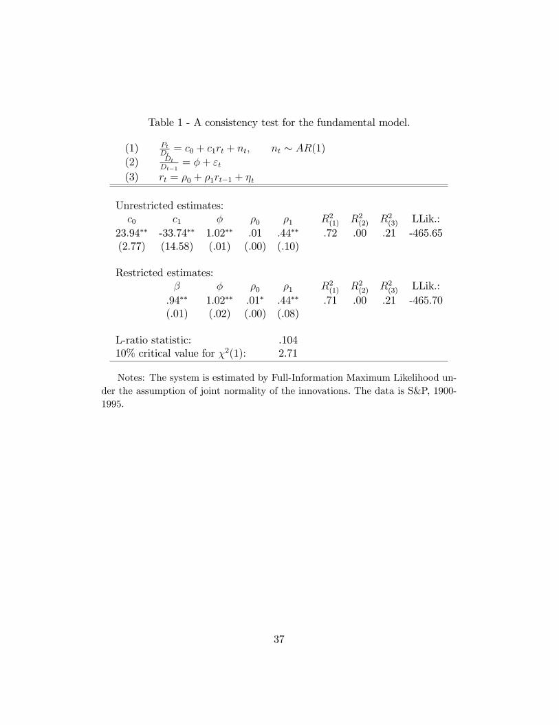
Table 1 - A consistency test for the fundamental model.

(1) PtDt= c0 + c1rt + nt; nt � AR(1)

(2) DtDt�1

= �+ "t(3) rt = �0 + �1rt�1 + �t

Unrestricted estimates:c0 c1 � �0 �1 R2(1) R2(2) R2(3) LLik.:

23.94�� -33.74�� 1.02�� .01 .44�� .72 .00 .21 -465.65(2.77) (14.58) (.01) (.00) (.10)

Restricted estimates:� � �0 �1 R2(1) R2(2) R2(3) LLik.:.94�� 1.02�� .01� .44�� .71 .00 .21 -465.70(.01) (.02) (.00) (.08)

L-ratio statistic: .10410% critical value for �2(1): 2.71

Notes: The system is estimated by Full-Information Maximum Likelihood un-der the assumption of joint normality of the innovations. The data is S&P, 1900-1995.

37

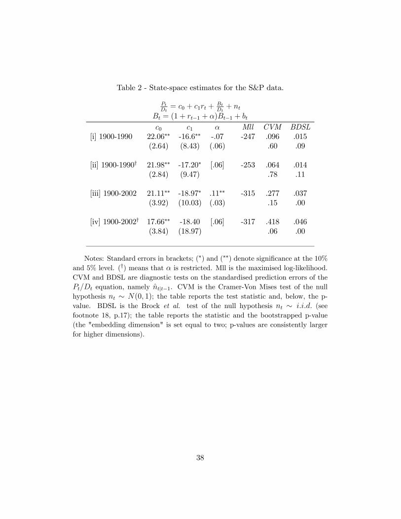
Table 2 - State-space estimates for the S&P data.

PtDt= c0 + c1rt +

BtDt+ nt

Bt = (1 + rt�1 + �)Bt�1 + bt

c0 c1 � Mll CVM BDSL[i] 1900-1990 22.06�� -16.6�� -.07 -247 .096 .015

(2.64) (8.43) (.06) .60 .09

[ii] 1900-1990y 21.98�� -17.20� [.06] -253 .064 .014(2.84) (9.47) .78 .11

[iii] 1900-2002 21.11�� -18.97� .11�� -315 .277 .037(3.92) (10.03) (.03) .15 .00

[iv] 1900-2002y 17.66�� -18.40 [.06] -317 .418 .046(3.84) (18.97) .06 .00

Notes: Standard errors in brackets; (�) and (��) denote signi�cance at the 10%and 5% level. (y) means that � is restricted. Mll is the maximised log-likelihood.CVM and BDSL are diagnostic tests on the standardised prediction errors of thePt=Dt equation, namely ntjt�1. CVM is the Cramer-Von Mises test of the nullhypothesis nt � N(0; 1); the table reports the test statistic and, below, the p-value. BDSL is the Brock et al. test of the null hypothesis nt � i:i:d: (seefootnote 18, p.17); the table reports the statistic and the bootstrapped p-value(the "embedding dimension" is set equal to two; p-values are consistently largerfor higher dimensions).

38

Table 3 - Price-dividend ratio equation, non-adjusted industry data.

Pt=Dt = c0 + c1rt + nt

c0 c1 R2 DW

1900-2000 31.77�� -35.44� .71 2.01(10.31) (19.79)

1900-1990 26.10�� -39.35� .67 2.02(4.51) (21.50)

1900-1970 28.22�� -31.53� .67 1.91(9.31) (16.04)

Notes: All equations estimated by 2sls; nt � AR(i), where the choice ofi = 1; 2; 3 is data-driven. Newey-West standard errors in brackets (truncation atlag 3).

Table 4 - Price-dividend ratio equation, adjusted industry data.

P at =Dat = c0 + c1rt + nt

c0 c1 R2 DW

1900-2000 18.92�� -18.06� .80 2.02(2.29) (10.83)

1900-1990 17.73�� -16.35 .82 2.03(2.73) (10.62)

1900-1970 19.67�� -18.58� .77 1.90(3.58) (10.67)

Notes: All equations estimated by ordinary least squares; nt � AR(i), wherethe choice of i = 1; 2; 3 is data-driven. Newey-West standard errors in brackets(truncation at lag 3). Two dummy variables are introduced for 1929 and 1971;they are both positive and signi�cant at the 1% level.

39

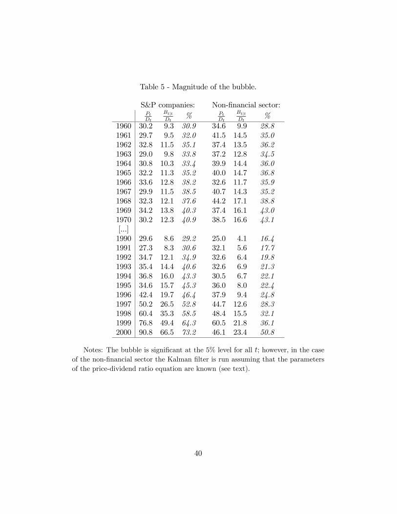
Table 5 - Magnitude of the bubble.

S&P companies: Non-�nancial sector:PtDt

BtjtDt

% PtDt

BtjtDt

%1960 30.2 9.3 30.9 34.6 9.9 28.81961 29.7 9.5 32.0 41.5 14.5 35.01962 32.8 11.5 35.1 37.4 13.5 36.21963 29.0 9.8 33.8 37.2 12.8 34.51964 30.8 10.3 33.4 39.9 14.4 36.01965 32.2 11.3 35.2 40.0 14.7 36.81966 33.6 12.8 38.2 32.6 11.7 35.91967 29.9 11.5 38.5 40.7 14.3 35.21968 32.3 12.1 37.6 44.2 17.1 38.81969 34.2 13.8 40.3 37.4 16.1 43.01970 30.2 12.3 40.9 38.5 16.6 43.1[...]1990 29.6 8.6 29.2 25.0 4.1 16.41991 27.3 8.3 30.6 32.1 5.6 17.71992 34.7 12.1 34.9 32.6 6.4 19.81993 35.4 14.4 40.6 32.6 6.9 21.31994 36.8 16.0 43.3 30.5 6.7 22.11995 34.6 15.7 45.3 36.0 8.0 22.41996 42.4 19.7 46.4 37.9 9.4 24.81997 50.2 26.5 52.8 44.7 12.6 28.31998 60.4 35.3 58.5 48.4 15.5 32.11999 76.8 49.4 64.3 60.5 21.8 36.12000 90.8 66.5 73.2 46.1 23.4 50.8

Notes: The bubble is signi�cant at the 5% level for all t; however, in the caseof the non-�nancial sector the Kalman �lter is run assuming that the parametersof the price-dividend ratio equation are known (see text).

40

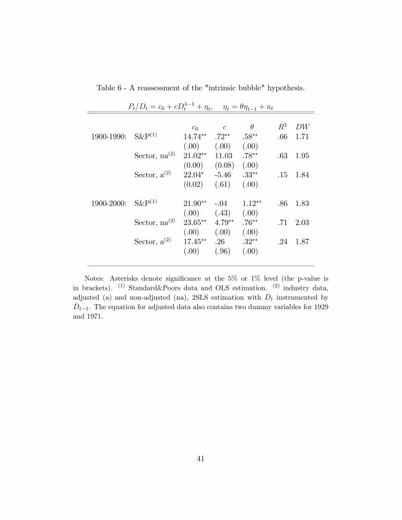
Table 6 - A reassessment of the "intrinsic bubble" hypothesis.

Pt=Dt = c0 + cD��1t + �t; �t = ��t�1 + ut

c0 c � R2 DW1900-1990: S&P(1) 14.74�� .72�� .58�� .66 1.71

(.00) (.00) (.00)Sector, na(2) 21.02�� 11.03 .78�� .63 1.95

(0.00) (0.08) (.00)Sector, a(2) 22.04� -5.46 .33�� .15 1.84

(0.02) (.61) (.00)

1900-2000: S&P(1) 21.90�� -.04 1.12�� .86 1.83(.00) (.43) (.00)

Sector, na(2) 23.65�� 4.79�� .76�� .71 2.03(.00) (.00) (.00)

Sector, a(2) 17.45�� .26 .32�� .24 1.87(.00) (.96) (.00)

Notes: Asterisks denote signi�cance at the 5% or 1% level (the p-value isin brackets). (1) Standard&Poors data and OLS estimation. (2) industry data,adjusted (a) and non-adjusted (na), 2SLS estimation with Dt instrumented byDt�1. The equation for adjusted data also contains two dummy variables for 1929and 1971.

41

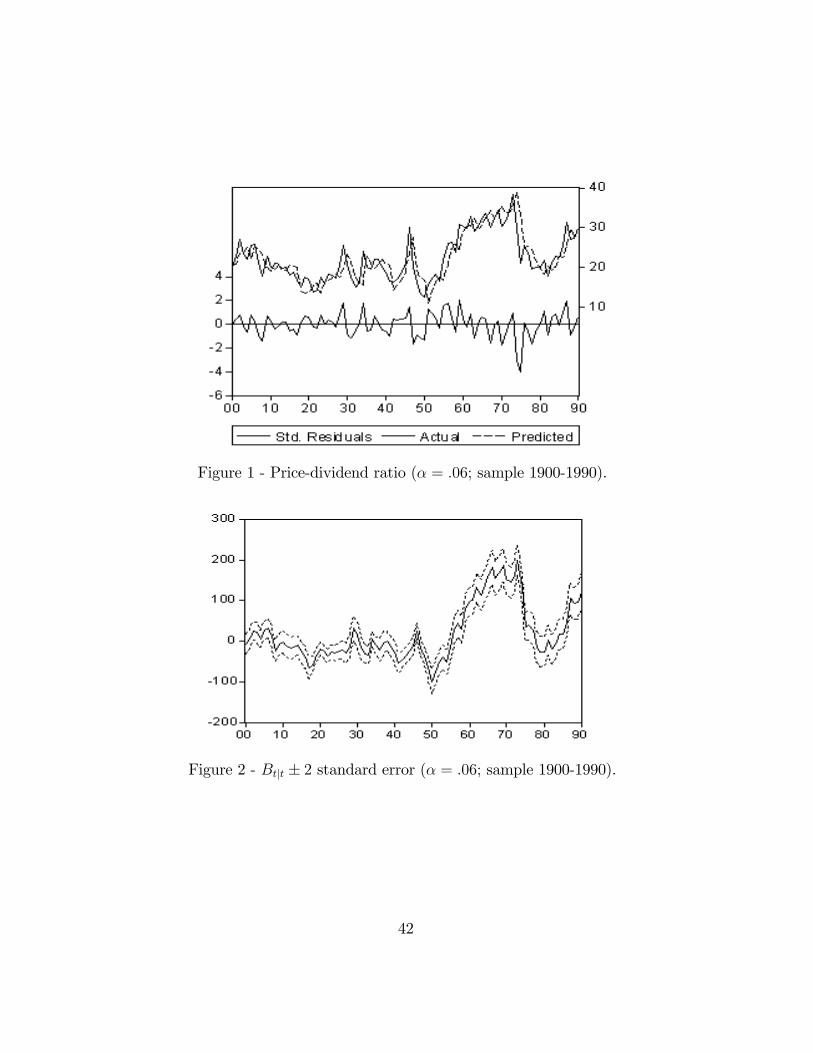
Figure 1 - Price-dividend ratio (� = :06; sample 1900-1990).

Figure 2 - Btjt � 2 standard error (� = :06; sample 1900-1990).

42

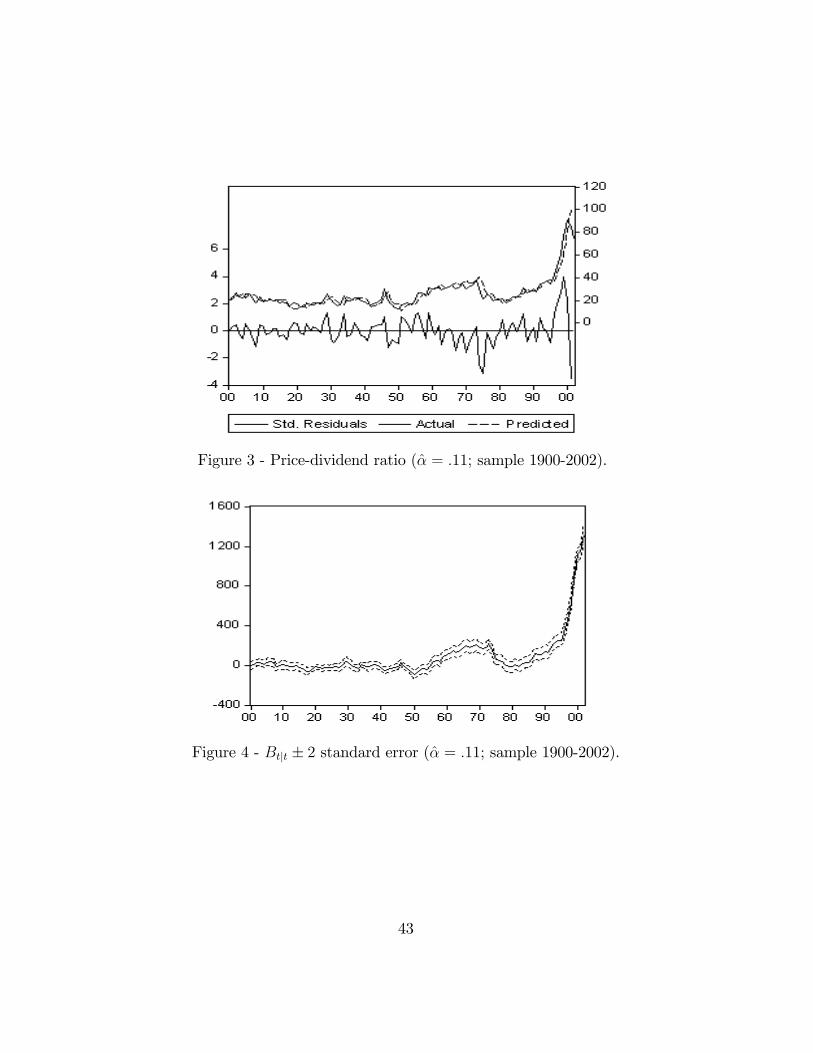
Figure 3 - Price-dividend ratio (� = :11; sample 1900-2002).

Figure 4 - Btjt � 2 standard error (� = :11; sample 1900-2002).

43

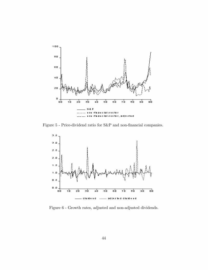
Figure 5 - Price-dividend ratio for S&P and non-�nancial companies.

Figure 6 - Growth rates, adjusted and non-adjusted dividends.

44

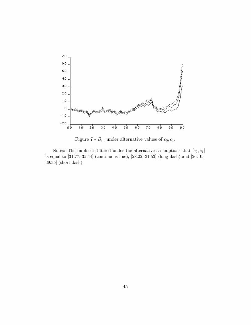
Figure 7 - Btjt under alternative values of c0; c1.

Notes: The bubble is �ltered under the alternative assumptions that [c0; c1]is equal to [31.77,-35.44] (continuous line), [28.22,-31.53] (long dash) and [26.10,-39.35] (short dash).

45