Coventry Polytechnic

Computer Simulation of Fractal Patterns

A project submitted for the degree of Bachelor of Engineering (Hons)

by M. R. Shaheedullah

Submitted: April 1989

Department of Applied Physical Science

Abstract Computer simulations have already been carried out which show that diffusion limited growth processes produce self-similar patterns. Fractal geometry defines self-similar patterns as having fractional dimensions and the patterns are hence termed fractals. Development of known models was carried out in an attempt to produce a more realistic simulation of diffusion limited growth processes, with specific reference to electro-deposition. New features included in the developed models include growth of more than one cluster and complete coverage of the substrate. Patterns and data were produced from which fractional dimensions could be calculated. The fractional dimensions calculated were between one and two which was as expected. Unexpected results were also observed. For the two developed models, it was found that the relationship between log of density and log of characteristic length deviated from its mathematically predicted linearity. It was concluded that this deviation was the result of impingement with the boundary and possibly between growing clusters.

1

Contents 1 INTRODUCTION TO FRACTAL GROWTH .......................................................................... 2

1.1 FRACTAL GEOMETRY ............................................................................................................. 2 1.2 SELF-SIMILARITY ................................................................................................................... 3 1.3 THE FRACTAL DIMENSION ..................................................................................................... 4

1.3.1 Introduction ...................................................................................................................... 4 1.3.2 Quantitative Consideration of Fractal Dimension ........................................................... 6

1.4 AIMS OF THIS PROJECT .......................................................................................................... 8

2 EXPERIMENTAL PROCEDURE ............................................................................................ 10

2.1 PARAMETERS ....................................................................................................................... 10 2.2 PROGRAMMING STRATEGY .................................................................................................. 11

3 EXPERIMENTS AND RESULTS ............................................................................................ 12

3.1 DLA MODEL 1 (SQUARE PERIMETER, ONE SET SEED) ......................................................... 12 3.1.1 Description of Model ...................................................................................................... 12 3.1.2 Description of Results ..................................................................................................... 13 3.1.3 Screen Prints................................................................................................................... 14 3.1.4 Data of No. Centres, Characteristic Length and Time ................................................... 15 3.1.5 Plot of ln(ρ) versus ln(L) ................................................................................................. 16 3.1.6 Plot of Fractional Coverage versus Time ....................................................................... 16 3.1.7 Program .......................................................................................................................... 17

3.2 DLA MODEL 2 (ONE RANDOM SEED) .................................................................................. 19 3.2.1 Description of the Model ................................................................................................ 19 3.2.2 Description of Results ..................................................................................................... 20 3.2.3 Screen Prints................................................................................................................... 21 3.2.4 Data of No. Centres, Characteristic Length and Time ................................................... 22 3.2.5 Plot of ln(ρ) versus ln(L) ................................................................................................. 23 3.2.6 .............................................................................................................................................. 23 3.2.7 Program .......................................................................................................................... 24

3.3 DLA MODEL 3 (MORE THAN ONE SEED) ............................................................................. 26 3.3.1 Description of Model ...................................................................................................... 26 3.3.2 Description of Results ..................................................................................................... 27 3.3.3 Screen prints ................................................................................................................... 28 3.3.4 Data of No. Centres, Characteristic Length and Time ................................................... 29 3.3.5 Plot of ln(ρ) versus ln(L) ................................................................................................. 30 3.3.6 Plot of fractional Coverage versus Time ........................................................................ 30 3.3.7 Program .......................................................................................................................... 31

4 DISCUSSION .............................................................................................................................. 33

4.1 DISCUSSION OF RESULTS ..................................................................................................... 33 4.2 DEVELOPMENTS ................................................................................................................... 34

5 CONCLUSIONS ......................................................................................................................... 35

6 ACKNOWLEDGEMENTS........................................................................................................ 36

7 REFERENCES ............................................................................................................................ 37

2

1 Introduction To Fractal Growth 1.1 Fractal Geometry

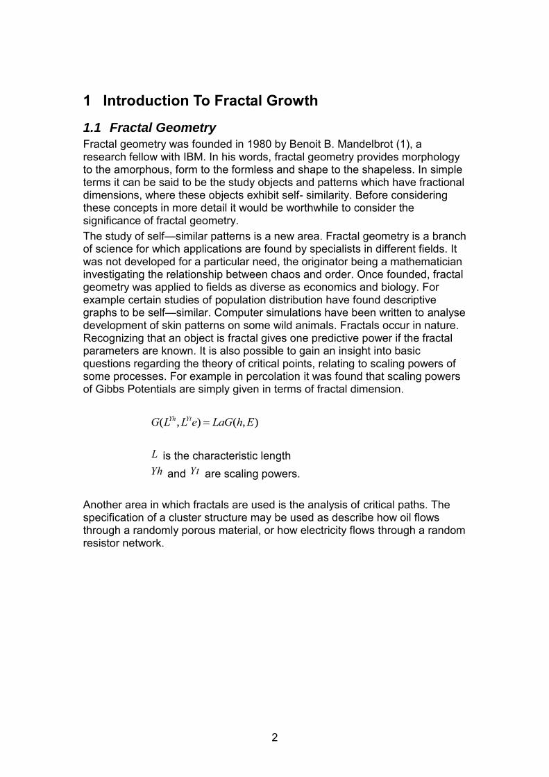
Fractal geometry was founded in 1980 by Benoit B. Mandelbrot (1), a research fellow with IBM. In his words, fractal geometry provides morphology to the amorphous, form to the formless and shape to the shapeless. In simple terms it can be said to be the study objects and patterns which have fractional dimensions, where these objects exhibit self- similarity. Before considering these concepts in more detail it would be worthwhile to consider the significance of fractal geometry. The study of self—similar patterns is a new area. Fractal geometry is a branch of science for which applications are found by specialists in different fields. It was not developed for a particular need, the originator being a mathematician investigating the relationship between chaos and order. Once founded, fractal geometry was applied to fields as diverse as economics and biology. For example certain studies of population distribution have found descriptive graphs to be self—similar. Computer simulations have been written to analyse development of skin patterns on some wild animals. Fractals occur in nature. Recognizing that an object is fractal gives one predictive power if the fractal parameters are known. It is also possible to gain an insight into basic questions regarding the theory of critical points, relating to scaling powers of some processes. For example in percolation it was found that scaling powers of Gibbs Potentials are simply given in terms of fractal dimension.

( , ) ( , )Yh YtG L L e LaG h E

L is the characteristic length Yh and Yt are scaling powers.

Another area in which fractals are used is the analysis of critical paths. The specification of a cluster structure may be used as describe how oil flows through a randomly porous material, or how electricity flows through a random resistor network.

3

1.2 Self-Similarity

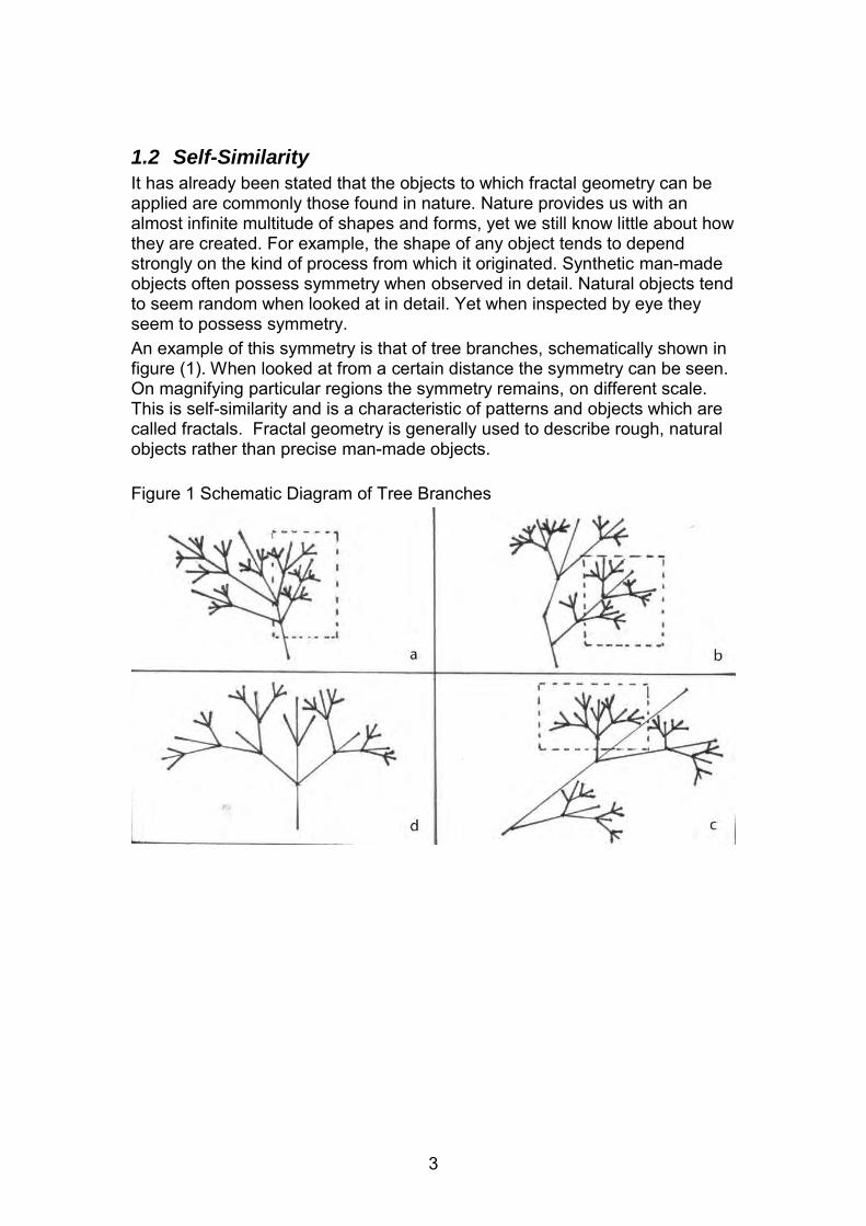
It has already been stated that the objects to which fractal geometry can be applied are commonly those found in nature. Nature provides us with an almost infinite multitude of shapes and forms, yet we still know little about how they are created. For example, the shape of any object tends to depend strongly on the kind of process from which it originated. Synthetic man-made objects often possess symmetry when observed in detail. Natural objects tend to seem random when looked at in detail. Yet when inspected by eye they seem to possess symmetry. An example of this symmetry is that of tree branches, schematically shown in figure (1). When looked at from a certain distance the symmetry can be seen. On magnifying particular regions the symmetry remains, on different scale. This is self-similarity and is a characteristic of patterns and objects which are called fractals. Fractal geometry is generally used to describe rough, natural objects rather than precise man-made objects. Figure 1 Schematic Diagram of Tree Branches

4

1.3 The Fractal Dimension

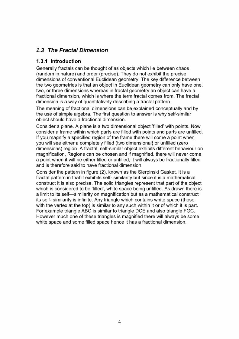
1.3.1 Introduction Generally fractals can be thought of as objects which lie between chaos (random in nature) and order (precise). They do not exhibit the precise dimensions of conventional Euclidean geometry. The key difference between the two geometries is that an object in Euclidean geometry can only have one, two, or three dimensions whereas in fractal geometry an object can have a fractional dimension, which is where the term fractal comes from. The fractal dimension is a way of quantitatively describing a fractal pattern. The meaning of fractional dimensions can be explained conceptually and by the use of simple algebra. The first question to answer is why self-similar object should have a fractional dimension. Consider a plane. A plane is a two dimensional object ’filled’ with points. Now consider a frame within which parts are filled with points and parts are unfilled. If you magnify a specified region of the frame there will come a point when you will see either a completely filled (two dimensional} or unfilled (zero dimensions) region. A fractal, self-similar object exhibits different behaviour on magnification. Regions can be chosen and if magnified, there will never come a point when it will be either filled or unfilled, it will always be fractionally filled and is therefore said to have fractional dimension. Consider the pattern in figure (2), known as the Sierpinski Gasket. It is a fractal pattern in that it exhibits self- similarity but since it is a mathematical construct it is also precise. The solid triangles represent that part of the object which is considered to be ’filled’, white space being unfilled. As drawn there is a limit to its self—similarity on magnification but as a mathematical construct its self- similarity is infinite. Any triangle which contains white space (those with the vertex at the top) is similar to any such within it or of which it is part. For example triangle ABC is similar to triangle DCE and also triangle FGC. However much one of these triangles is magnified there will always be some white space and some filled space hence it has a fractional dimension.

5

Figure 2 The Sierpinski Gasket

6

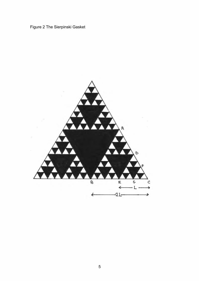
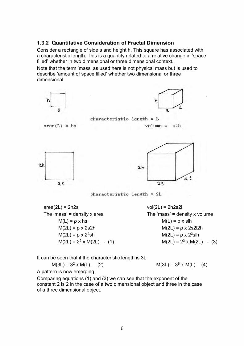
1.3.2 Quantitative Consideration of Fractal Dimension Consider a rectangle of side s and height h. This square has associated with a characteristic length. This is a quantity related to a relative change in ’space filled’ whether in two dimensional or three dimensional context. Note that the term ’mass’ as used here is not physical mass but is used to describe ’amount of space filled’ whether two dimensional or three dimensional.

It can be seen that if the characteristic length is 3L

M(3L) = 32 x M(L) - - (2) M(3L) = 38 x M(L) – (4) A pattern is now emerging. Comparing equations (1) and (3) we can see that the exponent of the constant 2 is 2 in the case of a two dimensional object and three in the case of a three dimensional object.

area(2L) = 2h2s The ‘mass’ = density x area

M(L) = ρ x hs M(2L) = ρ x 2s2h M(2L) = ρ x 22sh M(2L) = 22 x M(2L) - (1)

vol(2L) = 2h2s2l The ‘mass’ = density x volume

M(L) = ρ x slh M(2L) = ρ x 2s2l2h M(2L) = ρ x 23slh M(2L) = 23 x M(2L) - (3)

7

We can write that : M(2L) = 2d x M(L) where d is the dimension of the object

Comparing equations (2) and (4) we can see that where we have increased the characteristic length by a factor of 2 lthe coefficient of M(L) is 2 and where we have increased the characteristic length by a factor of three, the coefficient of M(L) is 3. We write that

M(λL) = λd x M(L) - (5) where λ is proportionate increase in characteristic length. The actual algebraic proof of this relationship requires the use of functional mathematics, which is beyond the scope of this project. In Euclidean geometry d can only be 1,2 or 3 for any object but we shall see that in fractal geometry d can be a fraction. Consider again the Sierpinski gasket figure (2). Let us define triangle DEC as having a characteristic length of L in which case triangle ABC has a characteristic length of 2L. The ’mass’ in this case depends on the number of filled and unfilled triangles. Since M is inversely proportional to the number of unfilled triangles we can compare M fort he triangles by counting the number of unfilled triangles. In triangle DEC the number of unfilled triangles is 9. In triangle ABC the number of unfilled triangles is 27. We can see that the ’mass’ of triangle ABC is 3 x mass of triangle DEC

M(2L) = 3 x M(L) If we compare this with equation (5)

M(λ L) = λd x M(L) We can see that λ = 2 and therefore 2d = 3. Taking logs d x ln(2) = ln3 so d = ln(3) - ln(2) which is the fractional dimension of the Sierpinski gasket. The general equation (5) above relates characteristic length to ’mass’. This applies where a change in L causes a change in the size of the frame of the fractal hence increasing the ’mass’, with the ’density’ being effectively fixed. However, as shall be seen later, it is sometimes more convenient to relate L to a change in density within a fixed frame. L can still be considered to be related to a change in amount of space filled but now in the context of a fixed frame whose ’mass’ is being increased.

8

It should be noted that in keeping the size of the frame fixed L can no longer be considered to be the length of a side of the frame in the case of a square. In fact we now need a new definition of L related to an increase in density. Let us consider the case where the fractal increases in mass within the frame. We know that

’mass’ α density In the case of a fixed frame with the mass increasing the density can be considered to be the fractional coverage of the frame therefore ’mass’ α fractional coverage and M α Ld so ρ= k x Ld so ln(ρ) = ln(k) + (d x ln(L)) If a graph of ln(ρ) versus ln(L) is drawn the gradient will be the fractal dimension. For certain growth processes assumptions can be made and rules specified as to how growth occurs. A model of the growth process can therefore be built and dynamically simulated on a computer. These are termed ’Cellular Automata’. Such models can lead to interesting patterns and data.

1.4 Aims of This Project

This project concentrates on computer simulations of models created to represent diffusion limited growth processes. The importance of diffusion (Brownian motion) in processes such as electro-deposition, colloidal aggregation and others has long been recognised. Only in recent years has it been practical to carry out computer simulations of aggregation processes of aggregation processes using Brownian ’random walk’ trajectories. A model in contemporary use is the diffusion-limited aggregation model. This was developed in recognition of the importance of diffusion in the above growth processes. The first of this type of work was carried by Finegold (2). however, the simulations were carried out on a small scale and no quantitative results were reported.

9

The event which contributed most to this area was a discovery by Witten and Sander (3). This was that a model based on a diffusion-limited growth process in which particles are added, one at a time, to a growing cluster or aggregate of particles leads to a fractal, self-similar structure. Because of its relevance to a wide variety of physical processes including dendritic growth, fluid-fluid displacement, colloidal aggregation and dielectric breakdown this model has generated considerable enthusiasm and has been extensively investigated during the last few years. It is proposed to develop the Witten-Sander model to be a more realistic simulation of diffusion limited growth processes. The particular process chosen to be the basis for the simulation is electro-deposition because it is a relatively simple two dimensional surface process. The development will be approached by creating a standard Witten-Sander model on a computer system, then modifying the system to incorporate changes in the model.

10

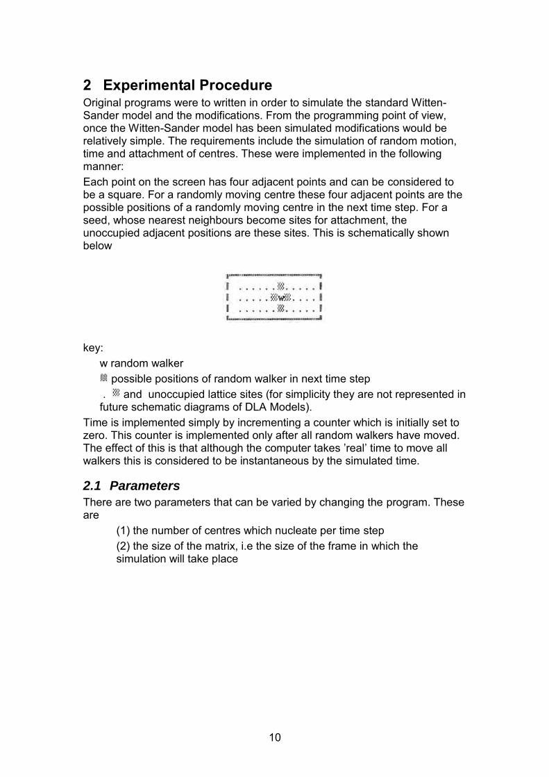
2 Experimental Procedure Original programs were to written in order to simulate the standard Witten-Sander model and the modifications. From the programming point of view, once the Witten-Sander model has been simulated modifications would be relatively simple. The requirements include the simulation of random motion, time and attachment of centres. These were implemented in the following manner: Each point on the screen has four adjacent points and can be considered to be a square. For a randomly moving centre these four adjacent points are the possible positions of a randomly moving centre in the next time step. For a seed, whose nearest neighbours become sites for attachment, the unoccupied adjacent positions are these sites. This is schematically shown below

key:

w random walker possible positions of random walker in next time step

. and unoccupied lattice sites (for simplicity they are not represented in future schematic diagrams of DLA Models).

Time is implemented simply by incrementing a counter which is initially set to zero. This counter is implemented only after all random walkers have moved. The effect of this is that although the computer takes ’real’ time to move all walkers this is considered to be instantaneous by the simulated time.

2.1 Parameters

There are two parameters that can be varied by changing the program. These are

(1) the number of centres which nucleate per time step (2) the size of the matrix, i.e the size of the frame in which the simulation will take place

11

2.2 Programming Strategy

The major ’strategic’ consideration is the method of checking whether a moving centre has reached a growing cluster. One approach would be to check the nearest neighbours of the moving site against the positions of all fixed centres. If the check proved positive the moving centre would then undergo the procedure which would make it a fixed centre. The checking of nearest neighbours against fixed centres would have to be repeated for every moving centre each time they move. In the later stages of the simulation this would be a very time consuming process. A possibly much quicker method would be to move the centre and check whether the new position is a nearest neighbour of a fixed centre. In this case the checking would be against unoccupied nearest neighbours of fixed centres rather than fixed centres themselves. This should be much quicker since the number of unoccupied nearest neighbours would be much smaller than the number of fixed centres (except at the very beginning of the program).

12

3 Experiments and Results 3.1 DLA Model 1 (Square Perimeter, One Set Seed)

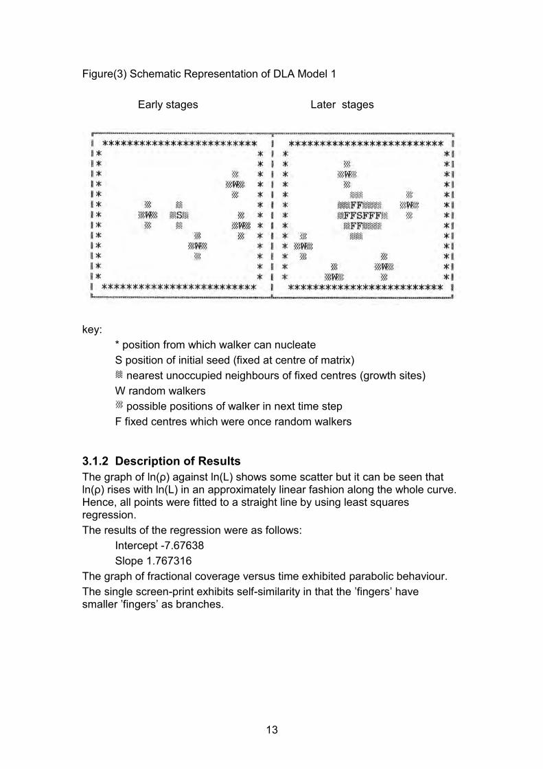
3.1.1 Description of Model The model is similar to the standard Witten-Sander DLA model but in this case the perimeter is a square not a circle. A perimeter is formed of adjacent sites in the shape of a square. In the middle of this square is a seed. We start with a square lattice and occupy the centre site with a seed particle. A particle is, randomly with time, then released into the lattice from the perimeter of the square. This particle executes a random walk until it reaches a neighbouring site of the seed particle upon which it ’sticks’ to the seed. The nearest neighbours of this centre become sites for growth. The model employs reflective boundary conditions, that is, when a random walker reaches an edge it is forced to continue its walk within the square. This process is repeated thousands of times until a large cluster is formed. A schematic diagram of the process is shown in figure(3). This model is an example of how totally random motion can give rise to self similar clusters. This is because the growth rule is non-local. The simulation ends when any part of the cluster reaches the perimeter since consideration of interference between the cluster and the perimeter is not included in the model.

13

Figure(3) Schematic Representation of DLA Model 1

key:

* position from which walker can nucleate S position of initial seed (fixed at centre of matrix)

nearest unoccupied neighbours of fixed centres (growth sites) W random walkers

possible positions of walker in next time step F fixed centres which were once random walkers

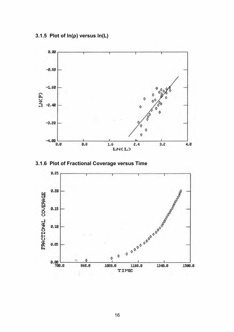
3.1.2 Description of Results The graph of ln(ρ) against ln(L) shows some scatter but it can be seen that ln(ρ) rises with ln(L) in an approximately linear fashion along the whole curve. Hence, all points were fitted to a straight line by using least squares regression. The results of the regression were as follows:

Intercept -7.67638 Slope 1.767316

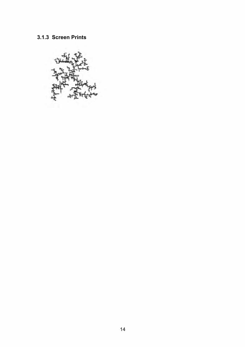
The graph of fractional coverage versus time exhibited parabolic behaviour. The single screen-print exhibits self-similarity in that the ’fingers’ have smaller ’fingers’ as branches.

Early stages Later stages

14

3.1.3 Screen Prints

15

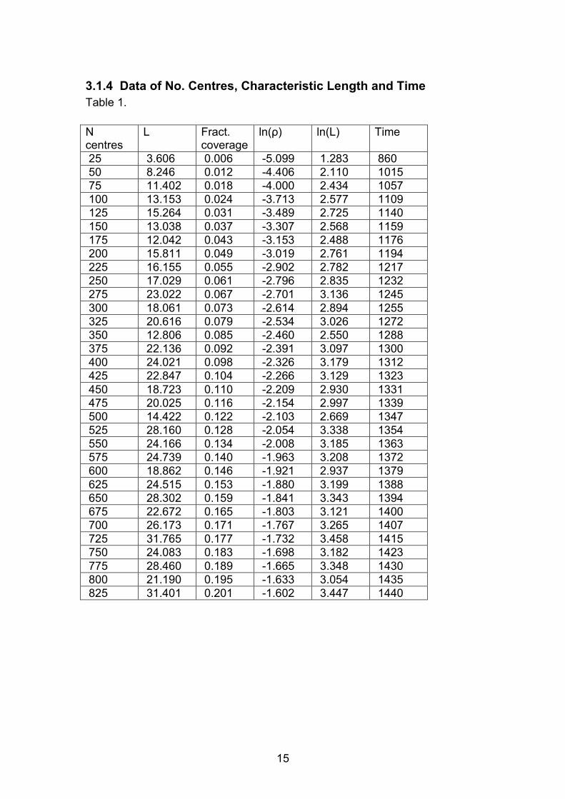
3.1.4 Data of No. Centres, Characteristic Length and Time Table 1. N centres

L Fract. coverage

ln(ρ) ln(L) Time

25 3.606 0.006 -5.099 1.283 860 50 8.246 0.012 -4.406 2.110 1015 75 11.402 0.018 -4.000 2.434 1057 100 13.153 0.024 -3.713 2.577 1109 125 15.264 0.031 -3.489 2.725 1140 150 13.038 0.037 -3.307 2.568 1159 175 12.042 0.043 -3.153 2.488 1176 200 15.811 0.049 -3.019 2.761 1194 225 16.155 0.055 -2.902 2.782 1217 250 17.029 0.061 -2.796 2.835 1232 275 23.022 0.067 -2.701 3.136 1245 300 18.061 0.073 -2.614 2.894 1255 325 20.616 0.079 -2.534 3.026 1272 350 12.806 0.085 -2.460 2.550 1288 375 22.136 0.092 -2.391 3.097 1300 400 24.021 0.098 -2.326 3.179 1312 425 22.847 0.104 -2.266 3.129 1323 450 18.723 0.110 -2.209 2.930 1331 475 20.025 0.116 -2.154 2.997 1339 500 14.422 0.122 -2.103 2.669 1347 525 28.160 0.128 -2.054 3.338 1354 550 24.166 0.134 -2.008 3.185 1363 575 24.739 0.140 -1.963 3.208 1372 600 18.862 0.146 -1.921 2.937 1379 625 24.515 0.153 -1.880 3.199 1388 650 28.302 0.159 -1.841 3.343 1394 675 22.672 0.165 -1.803 3.121 1400 700 26.173 0.171 -1.767 3.265 1407 725 31.765 0.177 -1.732 3.458 1415 750 24.083 0.183 -1.698 3.182 1423 775 28.460 0.189 -1.665 3.348 1430 800 21.190 0.195 -1.633 3.054 1435 825 31.401 0.201 -1.602 3.447 1440

16

3.1.5 Plot of ln(ρ) versus ln(L)

3.1.6 Plot of Fractional Coverage versus Time

17

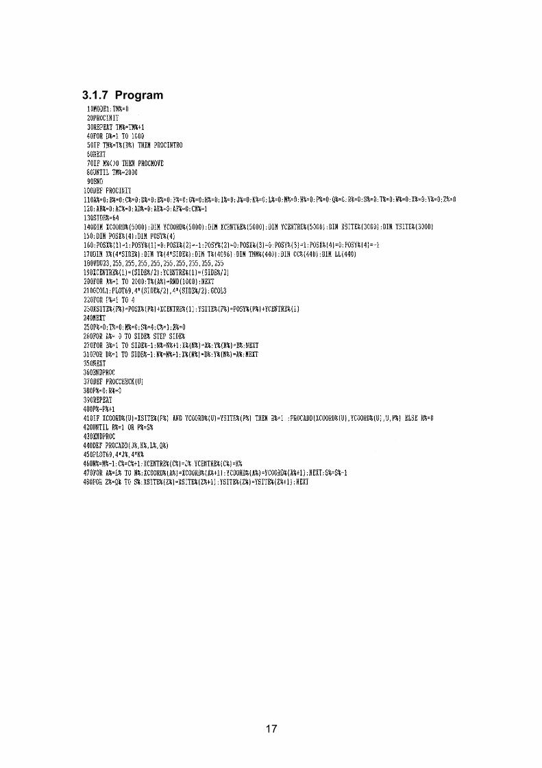
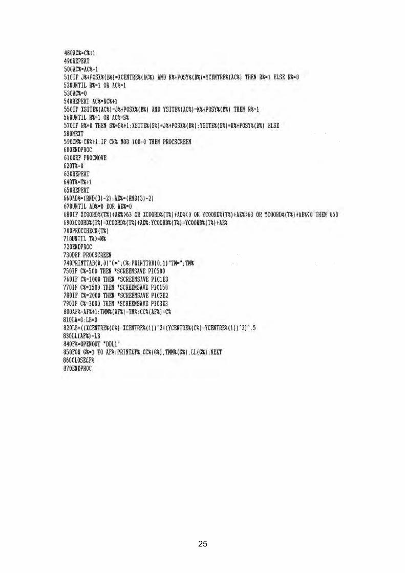
3.1.7 Program

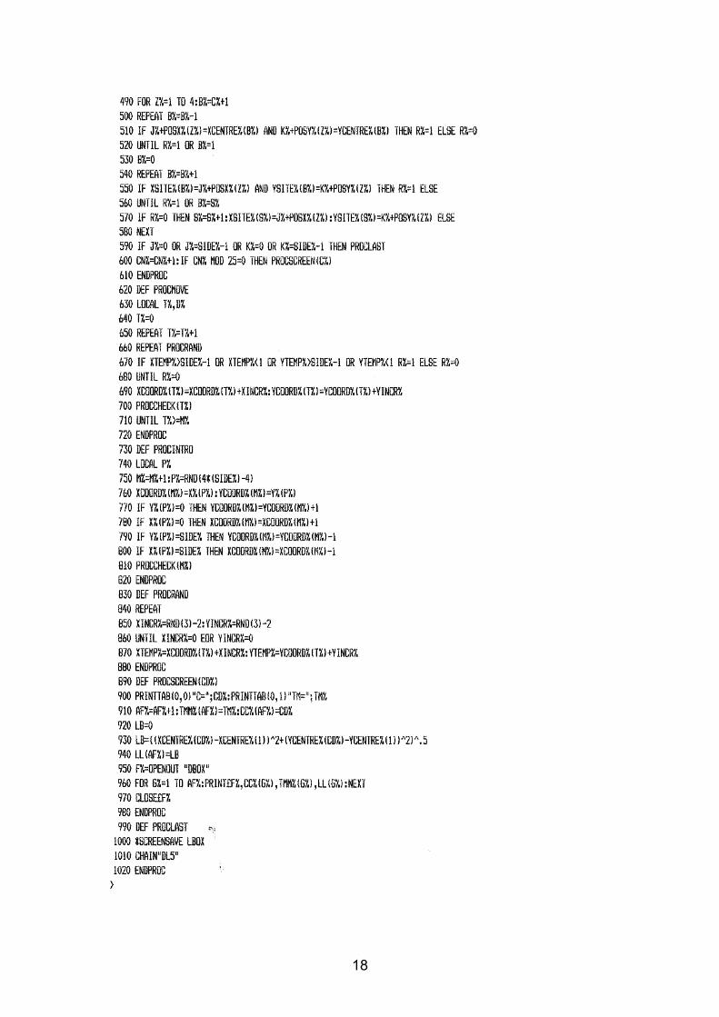
18

19

3.2 DLA Model 2 (One Random Seed)

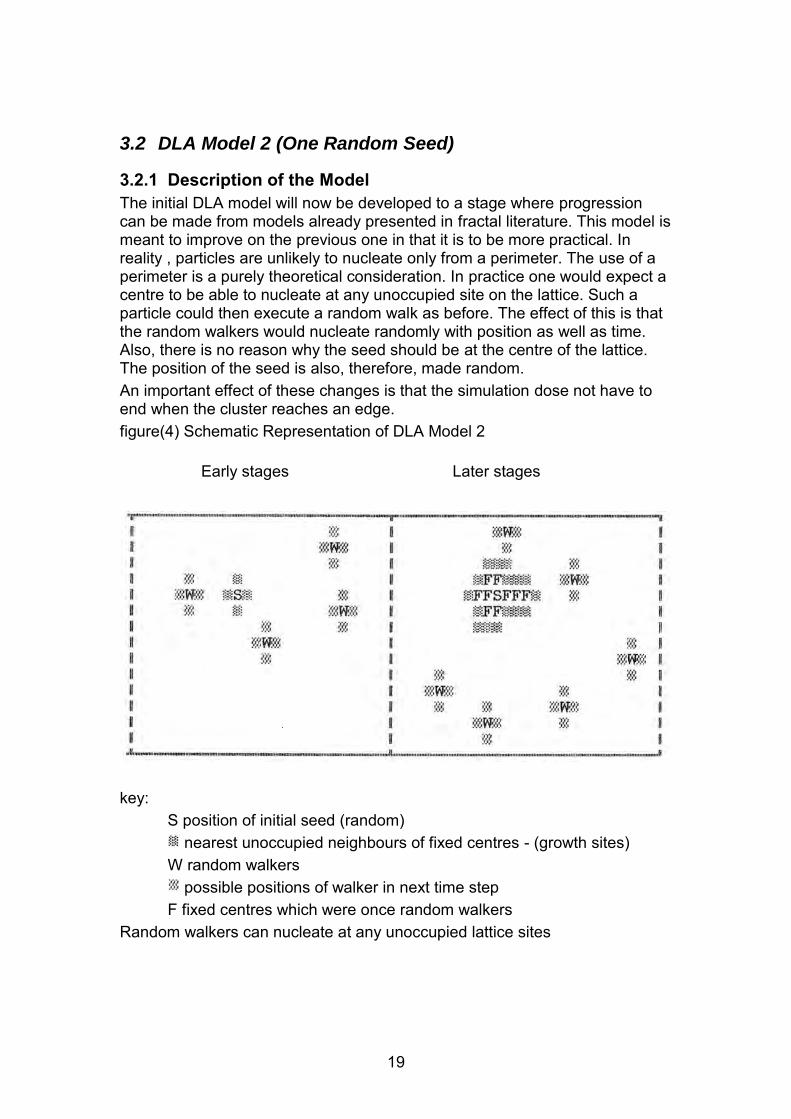
3.2.1 Description of the Model The initial DLA model will now be developed to a stage where progression can be made from models already presented in fractal literature. This model is meant to improve on the previous one in that it is to be more practical. In reality , particles are unlikely to nucleate only from a perimeter. The use of a perimeter is a purely theoretical consideration. In practice one would expect a centre to be able to nucleate at any unoccupied site on the lattice. Such a particle could then execute a random walk as before. The effect of this is that the random walkers would nucleate randomly with position as well as time. Also, there is no reason why the seed should be at the centre of the lattice. The position of the seed is also, therefore, made random. An important effect of these changes is that the simulation dose not have to end when the cluster reaches an edge. figure(4) Schematic Representation of DLA Model 2

key:

S position of initial seed (random) nearest unoccupied neighbours of fixed centres - (growth sites)

W random walkers possible positions of walker in next time step

F fixed centres which were once random walkers Random walkers can nucleate at any unoccupied lattice sites

Early stages Later stages

20

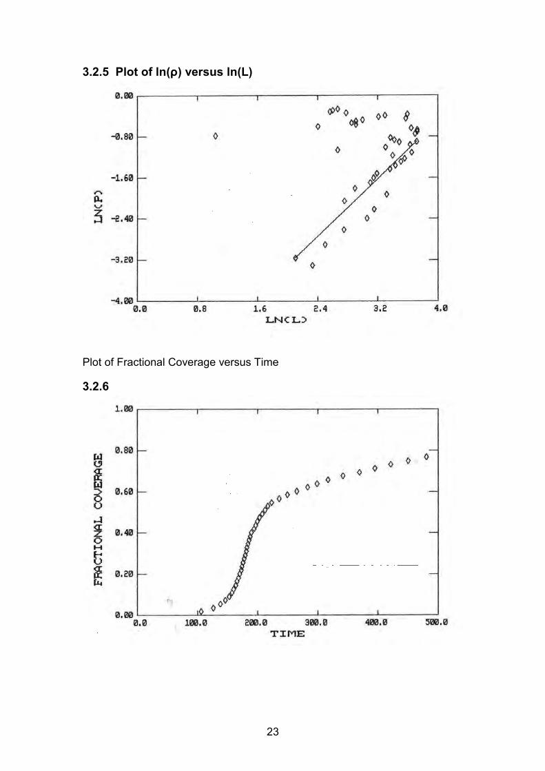
3.2.2 Description of Results From the data acquired two graphs were plotted. The first was a log-log plot of density versus characteristic length. Most of the curve is linear, i.e. ln(L) rise as ln(ρ) rises. The later portion of the graph is not linear. This is not due to an error in the simulation but is a characteristic of the relationship between the two quantities at the later stages of the simulation. Since the mathematical relationship from which the fractal dimension is calculated only holds for a linear % relationship between ln(L) and ln(ρ), regression is only applied to the linear portion of the graph. This linearity extends to a characteristic length of approximately 3.7. The results from the regression were:

Intercept -5 95484 Slope 1.315398

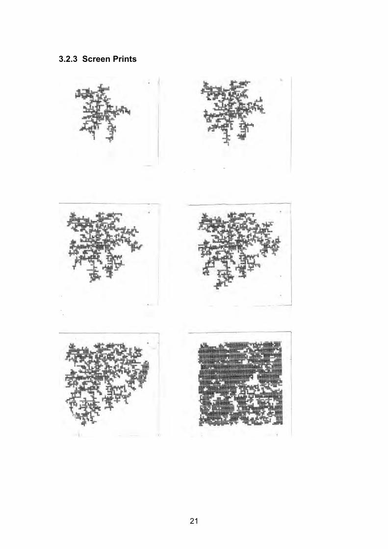
The fractional coverage were expected to vary in cumulative manner with respect to time and the graph does in fact exhibit parabolic behaviour. The screen prints of the patterns expected exhibit the q expected self-similarity which is most obvious when the number of centres is about 1000. In the later stages of the simulation when fractional coverage is quite high, self- similarity is less evident.

21

3.2.3 Screen Prints

22

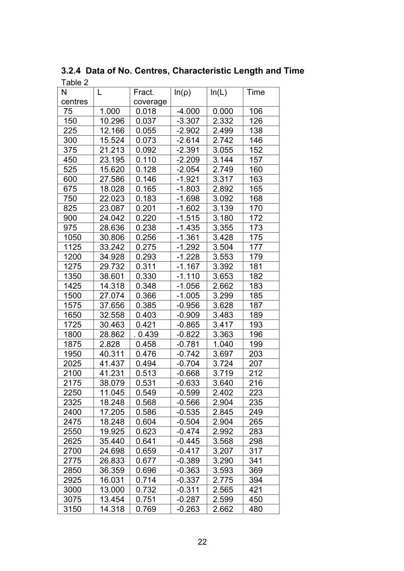
3.2.4 Data of No. Centres, Characteristic Length and Time Table 2 N centres

L Fract. coverage

ln(ρ) ln(L) Time

75 1.000 0.018 -4.000 0.000 106 150 10.296 0.037 -3.307 2.332 126 225 12.166 0.055 -2.902 2.499 138 300 15.524 0.073 -2.614 2.742 146 375 21.213 0.092 -2.391 3.055 152 450 23.195 0.110 -2.209 3.144 157 525 15.620 0.128 -2.054 2.749 160 600 27.586 0.146 -1.921 3.317 163 675 18.028 0.165 -1.803 2.892 165 750 22.023 0.183 -1.698 3.092 168 825 23.087 0.201 -1.602 3.139 170 900 24.042 0.220 -1.515 3.180 172 975 28.636 0.238 -1.435 3.355 173 1050 30.806 0.256 -1.361 3.428 175 1125 33.242 0.275 -1.292 3.504 177 1200 34.928 0.293 -1.228 3.553 179 1275 29.732 0.311 -1.167 3.392 181 1350 38.601 0.330 -1.110 3.653 182 1425 14.318 0.348 -1.056 2.662 183 1500 27.074 0.366 -1.005 3.299 185 1575 37.656 0.385 -0.956 3.628 187 1650 32.558 0.403 -0.909 3.483 189 1725 30.463 0.421 -0.865 3.417 193 1800 28.862 . 0.439 -0.822 3.363 196 1875 2.828 0.458 -0.781 1.040 199 1950 40.311 0.476 -0.742 3.697 203 2025 41.437 0.494 -0.704 3.724 207 2100 41.231 0.513 -0.668 3.719 212 2175 38.079 0.531 -0.633 3.640 216 2250 11.045 0.549 -0.599 2.402 223 2325 18.248 0.568 -0.566 2.904 235 2400 17.205 0.586 -0.535 2.845 249 2475 18.248 0.604 -0.504 2.904 265 2550 19.925 0.623 -0.474 2.992 283 2625 35.440 0.641 -0.445 3.568 298 2700 24.698 0.659 -0.417 3.207 317 2775 26.833 0.677 -0.389 3.290 341 2850 36.359 0.696 -0.363 3.593 369 2925 16.031 0.714 -0.337 2.775 394 3000 13.000 0.732 -0.311 2.565 421 3075 13.454 0.751 -0.287 2.599 450 3150 14.318 0.769 -0.263 2.662 480

23

3.2.5 Plot of ln(ρ) versus ln(L)

Plot of Fractional Coverage versus Time

3.2.6

24

3.2.7 Program

25

26

3.3 DLA Model 3 (More Than One Seed)

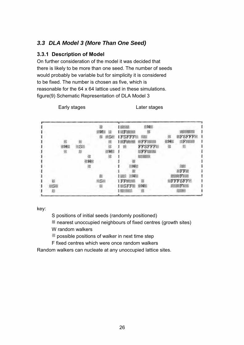
3.3.1 Description of Model On further consideration of the model it was decided that there is likely to be more than one seed. The number of seeds would probably be variable but for simplicity it is considered to be fixed. The number is chosen as five, which is reasonable for the 64 x 64 lattice used in these simulations. figure(9) Schematic Representation of DLA Model 3

key:

S positions of initial seeds (randomly positioned) nearest unoccupied neighbours of fixed centres (growth sites)

W random walkers possible positions of walker in next time step

F fixed centres which were once random walkers Random walkers can nucleate at any unoccupied lattice sites.

Early stages Later stages

27

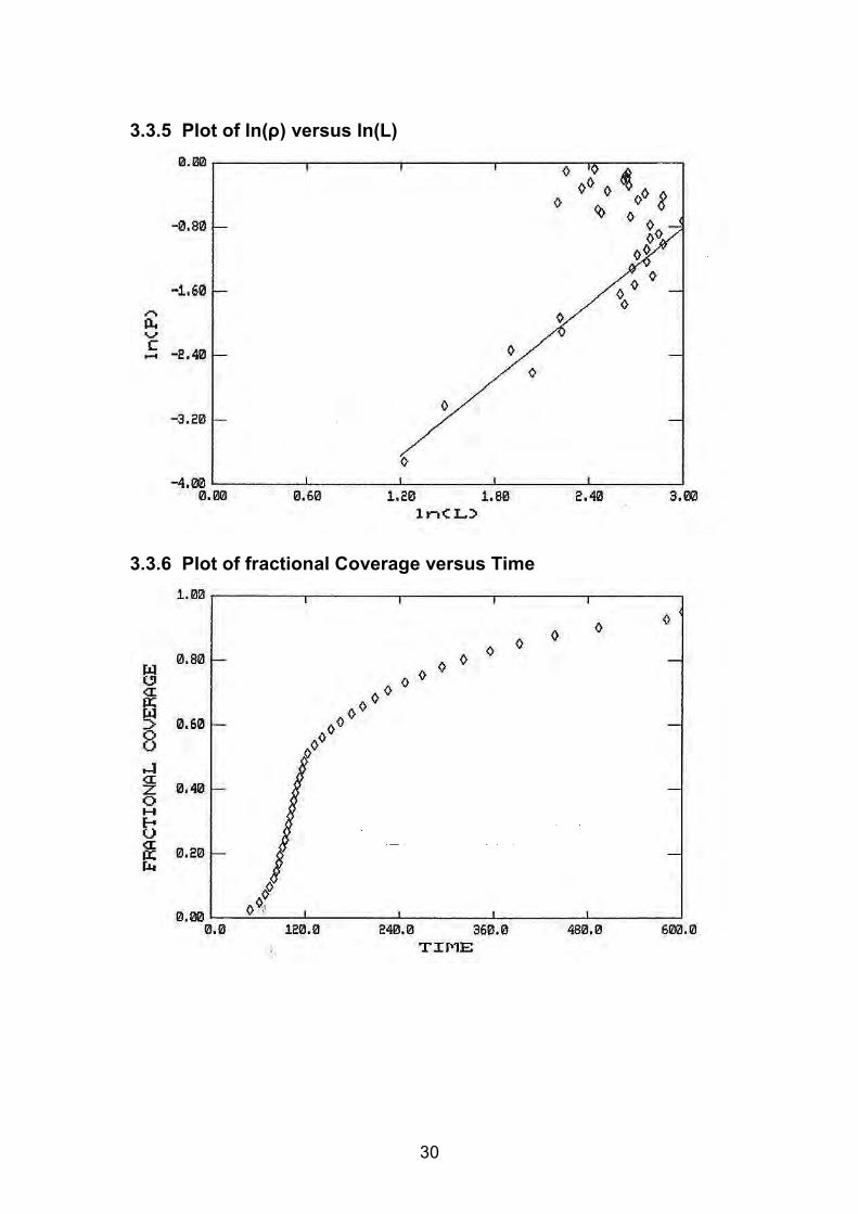
3.3.2 Description of Results The reasoning behind the regression of only the linear portion of the curve is similar to that for DLA Model 2, since the shape of the curve is very similar. This curve is, however, different in that the linear portion exhibits less scatter than the linear portions of similar graphs for the other two models. The linearity also ends earlier than that for DLA Model 2, at a characteristic length of about 2.8. The results of the regression were:

Intercept -5.531 Slope 1.572

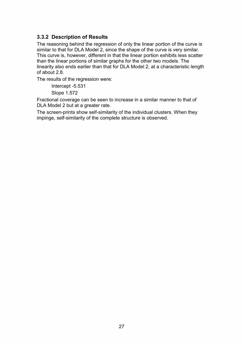
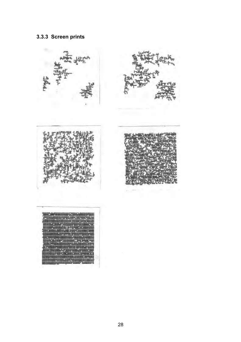
Fractional coverage can be seen to increase in a similar manner to that of DLA Model 2 but at a greater rate. The screen-prints show self-similarity of the individual clusters. When they impinge, self-similarity of the complete structure is observed.

28

3.3.3 Screen prints

29

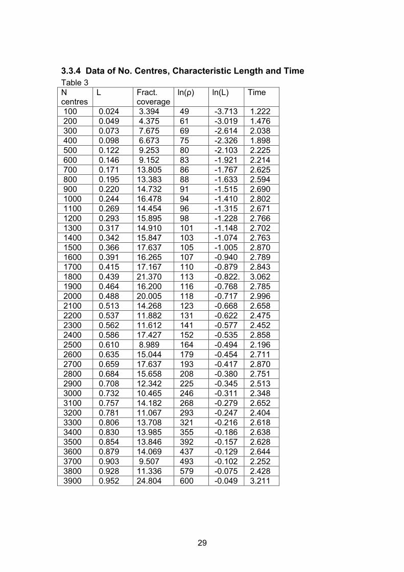
3.3.4 Data of No. Centres, Characteristic Length and Time Table 3 N centres

L Fract. coverage

ln(ρ) ln(L) Time

100 0.024 3.394 49 -3.713 1.222 200 0.049 4.375 61 -3.019 1.476 300 0.073 7.675 69 -2.614 2.038 400 0.098 6.673 75 -2.326 1.898 500 0.122 9.253 80 -2.103 2.225 600 0.146 9.152 83 -1.921 2.214 700 0.171 13.805 86 -1.767 2.625 800 0.195 13.383 88 -1.633 2.594 900 0.220 14.732 91 -1.515 2.690 1000 0.244 16.478 94 -1.410 2.802 1100 0.269 14.454 96 -1.315 2.671 1200 0.293 15.895 98 -1.228 2.766 1300 0.317 14.910 101 -1.148 2.702 1400 0.342 15.847 103 -1.074 2.763 1500 0.366 17.637 105 -1.005 2.870 1600 0.391 16.265 107 -0.940 2.789 1700 0.415 17.167 110 -0.879 2.843 1800 0.439 21.370 113 -0.822. 3.062 1900 0.464 16.200 116 -0.768 2.785 2000 0.488 20.005 118 -0.717 2.996 2100 0.513 14.268 123 -0.668 2.658 2200 0.537 11.882 131 -0.622 2.475 2300 0.562 11.612 141 -0.577 2.452 2400 0.586 17.427 152 -0.535 2.858 2500 0.610 8.989 164 -0.494 2.196 2600 0.635 15.044 179 -0.454 2.711 2700 0.659 17.637 193 -0.417 2.870 2800 0.684 15.658 208 -0.380 2.751 2900 0.708 12.342 225 -0.345 2.513 3000 0.732 10.465 246 -0.311 2.348 3100 0.757 14.182 268 -0.279 2.652 3200 0.781 11.067 293 -0.247 2.404 3300 0.806 13.708 321 -0.216 2.618 3400 0.830 13.985 355 -0.186 2.638 3500 0.854 13.846 392 -0.157 2.628 3600 0.879 14.069 437 -0.129 2.644 3700 0.903 9.507 493 -0.102 2.252 3800 0.928 11.336 579 -0.075 2.428 3900 0.952 24.804 600 -0.049 3.211

30

3.3.5 Plot of ln(ρ) versus ln(L)

3.3.6 Plot of fractional Coverage versus Time

31

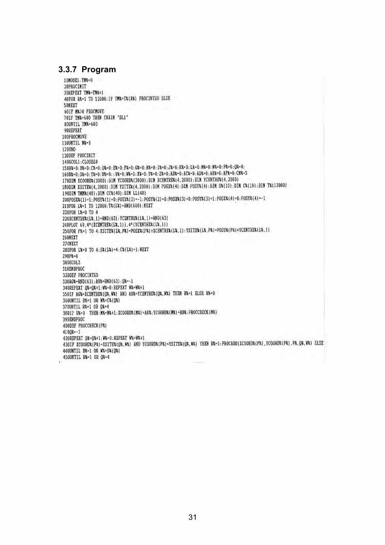
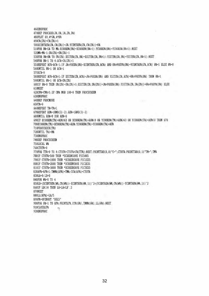
3.3.7 Program

32

33

4 Discussion 4.1 Discussion Of Results

The most important of the parameters investigated was the relationship between ln(ρ) and ln(L). The expected result was a linear relationship between ln(ρ) and 1n(L) which would give a positive gradient. This gradient would be the fractal dimension. The values of the fractal dimensions were expected to be between 1 and 2 since the pattern has a dimensionality of two, i.e. in a two dimensional context. The log-log plots of density versus characteristic length proved interesting. The earlier parts of the curve exhibit the expected linearity. Regression of this part gave the fractal dimension. However the later parts of the curve deviated significantly from the linear portion. This deviation was not random. The curve follows a perceivable path, arcing back, indicating that as ln(P} increases ln(L) decreases. This is behaviour not previously discussed in fractal literature. It occurs in models 2 and 3, not 1. There may two possible causes.

1) impingement with boundary (edges) 2) impingement between clusters in the case of model 3.

The scans of fractional coverage vs time were as expected.The exponential increase in the early part of the curve was expected, however, the later parts of the curve were new results. A possible explanation for this is that once the cluster reaches the boundary one would expect the rate coverage to decrease and eventually flatten out. This analysis is borne out by the fact that the scans for the Witten-Sander model consisted of only the exponential potion. The uniformity of the curves indicate that the scale of the model is large enough to provide meaningful results. That is, the number of centres, the size of the frame and the time were of adequate quantity. The fractal dimensions were as expected, values between 1 and 2. This helps validate the choice of characteristic length. Figures deviating from the expected dimensionality would indicate a misconception in the model with one likely cause being the characteristic length. The achieved results are significant in that they give quantitative results for previously unexplored models. The exact significance would require extensive mathematical analysis including theory of critical points which is beyond the scope of this project. One important way in which the developed models are different from the Witten-Sander model is that they allow complete i coverage of the substrate. This models therefore simulate the process when it is not diffusion controlled. In the later stages of the simulation the amount of free substrate is reduced. This means that the extent of random motion of the walkers before they become fixed is reduced. This decreases the effect of diffusion in the growth process until the fractional coverage is so great that only individual free sites are left on the substrate. After this the rate of growth is completely controlled by the rate of nucleation.

34

4.2 Developments

The models presented could be developed further. Modifications could include randomizing the number of seeds rather than keeping it fixed. The effect of impingement may also be investigated. This could concentrate on the difference between impingement of the cluster on the boundary and impingement between clusters. This could be done by forcing the seeds to be close to each other but far from the edges of the frame in one model and forcing the seeds to be close to the edges but far from each other in another. Further development could include more detailed consideration of what happens when two randomly walking particles meet. The possibility that they stick and move together could be investigated. After this moving cluster reached a certain size it could become stationary due to its increased mass. The most important development would be a more detailed analysis of the non-linear portion of the ln(ρ) ln(L) curve. This would require mathematical analysis. It may also be possible to calculate fractional dimensions for electro- deposition by mathematical of the physical quantities and compare the results with those acquired by computer simulations. This is a technique which has been used for simulations of other processes such as colloidal aggregation.

35

5 Conclusions 1) The fractal dimension of the standard Witten-Sander DLA model was found to be 1.8 2) The fractal dimension of DLA Model 2 (one random seed and random nucleation) was found to be 1.3 3) The fractal dimension of DLA Model 3 (five seeds and random nucleation) was found to be 1.6 4) The relationship between ln(ρ) and ln(L) for the standard Witten-Sander model did not deviate significantly from linearity. 5) The relationship between ln(ρ) and ln(L) for DLA Model 2 deviated at a value of approximately 3.7 for ln(L). 6) The relationship between ln(ρ) and ln(L) for DLA Model 3 deviated at a value of approximately 2.8 for ln(L).

36

6 Acknowledgements I would like to thank both my supervisors Dr M.Y. Abyaneh and Dr D. Kirk for their help and encouragement.

37

7 References 1) Mandelbrot, B.B., "The Fractal Geometry of Nature", W.H.Freeman, San Francisco (1982) 2) Finegold, L.X.. Biochem. Biophys. Acta 448,393 (1976) 3) Witten, T.A. and Sander, L.M., Phy. rev. lett., 47, 1400 (1981) 4) Stanley, H.E., and Ostrowsky, N., On Growth and Form, Fractal and Non-Fractal patterns in Physics, NATO ASI, (1985)g