Embed Size (px)
Citation preview

BS2243 – Lecture 4 Cournot duopoly and extensions
Spring 2012
(Dr. Sumon Bhaumik)

Cournot duopoly – market structure
• Two firms (A and B)
– Example: OPEC and non-OPEC oil producing countries
• Homogeneous product
• Competition in quantities
• Each firm assumes that the other firm will not react to its own choice of output

Cournot duopoly – strategic behaviour
• Firm behaviour • Reaction function
Market demand
Residual demand
qA qA1 qA2
£ qB
qA qA1 qA2
D D’ MR
MR’ MC

Cournot duopoly – Nash equilibrium
• Each firm’s output depends on the output choice of the other firm: Nash strategy
• At the quantity levels defined by the intersection of the two reaction functions, neither firm has any incentive to change output: equilibrium
qB
qA
Reaction function of Firm A
Reaction function of Firm B
qB1
qB2
qA1 qA2

Algebra of Cournot duopoly - I
• Inverse demand curve
P = 1000 – 10Q
• Two identical firms – Firm 1 produces q1 and Firm 2 produces q2
q1 + q2 = Q
• Cost structure
AC = MC = 50

Algebra of Cournot duopoly - II
• Profit maximising condition for a firm MC = MR
• Decision
– How much to produce?
• Rewriting inverse demand curve P = 1000 – 10(q1 + q2) P = 1000 – 10q1 – 10q2
• Marginal revenue curve Firm 1: (1000 – 10q2) – 20q1
Firm 2: (1000 – 10q1) – 20q2

Algebra of Cournot duopoly - III
• Profit maximisation Firm 1: (1000 – 10q2) – 20q1 = 50 20q1 + 10q2 = 950 (Verify: q1 = 47.5 – 0.5q2) Reaction function of Firm 1 Firm 2: (1000 – 10q1) – 20q2 = 50 10q1 + 20q2 = 950 (Verify: q2 = (95/2) – 0.5q1) Reaction function of Firm 2 • Nash equilibrium Solve the reaction functions simultaneously 20q1 + 10q2 = 950 10q1 + 20q2 = 950

Algebra of Cournot duopoly - IV
• Quantities in equilibrium Solving the reaction functions simultaneously q1 = , q2 =
• Price in equilibrium P = 1000 – 10(q1 + q2) =
• Profits in equilibrium 1 = (P – AC) x q1 = 2 = (P – AC) x q2 =

Strategy I – merger or collusion
• Market effectively has one multi-plant firm
– Firm 1 has become Plant 1, and Firm 2 has become Plant 2
• Decisions
– How much to produce?
– How to distribute the output between the two plants?

Strategy I – incidence of merger
0
100
200
300
400
500
600
700
800
900
1000
1990 1991 1992 1993 1994 1995 1996 1997 1998 1999 2000 2001 2002 2003 2004 2005 2006 2007 2008
M&A-UK-UK M&A-Overseas-UK M&A-UK-Overseas
Source: Office of National Statistics

Strategy I – intuition
• The multi-plant firm will set output at the level where MC = MR
• It will allocate a larger share of the output to the firm with the lower cost
• If the plants have identical cost structures, the optimum output will be equally divided between the two plants

Algebra for Strategy I – I
• Inverse demand curve P = 1000 – 10Q
• Two identical plants
– Plant 1 produces q1 and Plant 2 produces q2
q1 = q2 = Q/2
• Cost structure AC = MC = 50
• Profit maximising condition for a firm MC = MR 50 = 1000 – 20Q

Algebra for Strategy I – II
• Decisions – How much to produce? 1000 – 20Q = 50 20Q = 950 Q = 47.5
– How to distribute output between the two plants? q1 = q2 = Q/2 = 47.5/2 = 28.75
• Outcomes P = 1000 – 10Q = 1000 – (10 x 47.5) = 525 = (P – AC) x Q = (525 – 50) x 47.5 = In case of collusion, profit shared equally by the two firms

Strategy II – lobby for subsidy
http://blogs.wsj.com/environmentalcapital/2009/05/07/biofuels-bill-federal-subsidies-will-top-400-billion-enviros-say/tab/article/

Strategy II – impact of subsidy
• Subsidy reduces marginal cost of production
• The new marginal cost equals the marginal revenue at a higher output level
• The optimum output level
of the firm is higher
Market demand
Residual demand
qA
£
subsidy
MC
MC’

Algebra for Strategy II – I
• Inverse demand curve P = 1000 – 10Q
• Two identical firms
– Firm 1 produces q1 and Firm 2 produces q2
q1 + q2 = Q
• Firm 1 gets a subsidy of 10 per unit of output
• Cost structure Firm 1: AC = MC = 50 – 10 = 40 Firm 2: AC = MC = 50

Algebra of Strategy II - II
• Profit maximising condition for a firm MC = MR
• Decision
– How much to produce?
• Rewriting inverse demand curve P = 1000 – 10(q1 + q2) P = 1000 – 10q1 – 10q2
• Marginal revenue curve Firm 1: (1000 – 10q2) – 20q1
Firm 2: (1000 – 10q1) – 20q2

Algebra of Strategy II - III
• Profit maximisation Firm 1: (1000 – 10q2) – 20q1 = 40 20q1 + 10q2 = 960 (Verify: q1 = 48 – 0.5q2) Reaction function of Firm 1 Firm 2: (1000 – 10q1) – 20q2 = 50 10q1 + 20q2 = 950 Reaction function of Firm 2 • Nash equilibrium Solve the reaction functions simultaneously 20q1 + 10q2 = 960 10q1 + 20q2 = 950
Algebra of Strategy II - IV
• Quantities in equilibrium Solving the reaction functions simultaneously q1 = , q2 =
• Price in equilibrium P = 1000 – 10(q1 + q2) =
• Profits in equilibrium 1 = (P – AC) x q1 = 2 = (P – AC) x q2 =

Strategy III – become a Stackelberg leader
• Firm A (the Stackelberg leader) takes the strategic behaviour of Firm B into consideration
• Note the difference in the residual demand curve (relative to the Cournot competition scenario)
• In equilibrium, Firm A (the leader) would be better off and Firm B (the follower) would be worse off
Market demand
Residual demand
qA
£
MC
D
D’
MR’
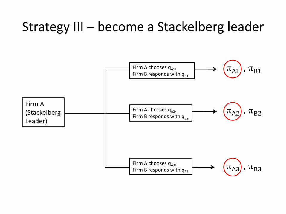
Strategy III – become a Stackelberg leader
Firm A (Stackelberg Leader)
Firm A chooses qA1, Firm B responds with qB1
Firm A chooses qA3, Firm B responds with qB3
Firm A chooses qA2, Firm B responds with qB2
A1 , B1
A2 , B2
A3 , B3
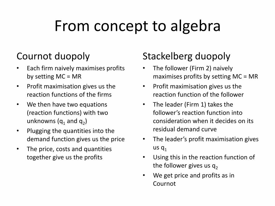
From concept to algebra
Cournot duopoly • Each firm naively maximises profits
by setting MC = MR
• Profit maximisation gives us the reaction functions of the firms
• We then have two equations (reaction functions) with two unknowns (q1 and q2)
• Plugging the quantities into the demand function gives us the price
• The price, costs and quantities together give us the profits
Stackelberg duopoly • The follower (Firm 2) naively
maximises profits by setting MC = MR
• Profit maximisation gives us the reaction function of the follower
• The leader (Firm 1) takes the follower’s reaction function into consideration when it decides on its residual demand curve
• The leader’s profit maximisation gives us q1
• Using this in the reaction function of the follower gives us q2
• We get price and profits as in Cournot

Algebra of Stackelberg duopoly - I
• Inverse demand curve P = 1000 – 10Q
• Two identical firms
– Firm 1 produces q1 and Firm 2 produces q2
q1 + q2 = Q – Firm 1 is Stackelberg leader
• Cost structure AC = MC = 50

Algebra of Stackelberg duopoly - II
• Profit maximisation of Firm 2
(1000 – 10q1) – 20q2 = 50 (from the algebra of Cournot)
10q1 + 20q2 = 950 (reaction function of Firm 2)
q2 = (950 – 10q1)/20 = 47.5 – 0.5q1
• Demand function of Firm 1
P = 1000 – 10q2 – 10q1
= 1000 – 10(47.5 - 0.5q1) – 10q1 = 525 – 5q1
• Profit maximisation of Firm 1
525 – 10q1 = 50

Algebra of Stackelberg duopoly - III
• Quantities in equilibrium First solve the profit maximisation problem of Firm 1 q1 = Then substitute q1 into the reaction function of Firm 2 q2 =
• Price in equilibrium P = 1000 – 10(q1 + q2) =
• Profits in equilibrium 1 = (P – AC) x q1 = 2 = (P – AC) x q2 =