Embed Size (px)
DESCRIPTION
This British Standard, a part of the BS 5400 series, recommends methods for the fatigue assessment of parts of bridges which are subject to repeated fluctuations of stress. Standard load spectra are given for both highway and railway bridges.The following alternative methods of fatigue assessment are described for both highway and railway bridges:a) simplified methods that are applicable to parts of bridges with classified details and which are subjected to standard loadings;b) methods using first principles that can be applied in all circumferences.
Citation preview
BRITISH STANDARD
Steel, concrete and composite bridges - Part 10: Code of practice for fatigue
ICS 93.040
NO COPYING WITHOUT BSI PERMISSION EXCEPT AS PERMITTED BY COPYRIGIW LAW
BS 5400 : Part 10 : 1980
Licensed copy:UNIVERSITY OF NOTTINGHAM, 17/11/2008, Uncontrolled Copy, © BSI

Issue 1, March 1999 BS 5400 : Part 10 : 1980
Summary of pages
The following table identifies the current issue of each page. lssue 1 indicates that a page has been introduced for the first time by amendment. Subsequent issue numbers indicate an updated page. Vertical sidelining on replacement pages indicates the most recent changes (amendment, addition, deletion).
Front cover h i d e front cover a b
d 1 2 3 4 4a 4b 5
C
Issue
2 blank 1 blank blank 1 2 2 2 2 1 blank 2
Page
6 7 to 42 43 44
49 50 51 52 53 54 Inside back cover Back cover
45 to da
Issue
Original original 2 original Original 2 blank 2 blank 2 blank original 2
a
Licensed copy:UNIVERSITY OF NOTTINGHAM, 17/11/2008, Uncontrolled Copy, © BSI
BS 5400 : Part 10 : 1 980 Issue 1, March 1999
Contents Page
Foreword 1 Cooperating organizations Back cover Recommendations 1. 1.1 1.2 1.3 1.4 1.5 1.5.1 1.5.2 1.5.3 2. 3. 3.1 3.2 4. 4.1 4.2
4.4 4.5 5. 5.1 5.1.1 5.1.2 5.2 5.2.1 5.2.2 5.3 5.3.1 5.3.2 5.4 6. 6.1 6.1.1 6.1.2 6.1.3
6.1.4 6.1.5 6.1.6 6.2 6.3
6.4
6.4.1 6.4.2 6.4.3 6.5 7. 7.1 7.2 7.2.1 7.2.2 7.2.3 7.2.4 7.2.5 7.3 7.3.1 7.3.2 7.3.3 8.
8.1 8.1.1 8.1.2 8.2
8.2.1
d
I 4.3
Scope General Loading Assessment procedures Other sources of fatigue damage Limitations Steel decks Reinforcement Shear connectors References Definitions and symbols Definitions Symbols General guidance Design life Classification and workmanship Stresses Methods of assessment Factors influencing fatigue behaviour Classification of details Classification General Classification of details in table 17 Unclassified details General Post-welding treatments Workmanship and inspection General Detrimental effects Steel decks Stress calculations General Stress range for welded details Stress range for welds Effective stress range for non-welded details Calculation of stresses Effects to be included Effects to be ignored Stress in parent metal Stress in weld throats other than those attaching shear connectors Stresses in welds attaching shear connectors General Stud connectors Channel and bar connectors Axial stress in bolts Loadings for fatigue assessment Design loadings Highway loading General Standard loading Application of loading Allowance for impact Centrifugal forces Railway loading General Application of loading Standard load spectra Fatigue assessment of highway bridges Methods of assessment General Simplified procedures Assessment without damage calculation General
2 2 2 2 2 2 2 2 2 2 2 2 3 3 3 3 4 4 3 4 4 4 4 4 4 4 4 4 4 4 4 4 4 4
4 4 5 5 5
5
6 6 6 6 6 6 6 6 6 6 6 8 8 8 8 8 10
12 12 12 12
12 12
8.2.2 8.2.3
8.3
8.3.1 8.3.2 8.4
8.4.1
8.4.3 8.4.4 9. 9.1 9.1.1 9.1.2 9.2 9.2.1 9.2.2 9.2.3 9.2.4 9.3 9.3.1 9.3.2 9.3.3
9.3.4 9.3.5 10.
11. 11.1 11.2 11.3 11.4 11.5
8.4.2
Page Procedure 12 Adjustment factors for an, class S details only 12 Damage calculation, single vehicle method 12 General 12 Procedure 12 Damage calculation, vehicle spectrum method 14 General 14 Design spectrum 14 Simplification of design spectrum 14 Calculation of damage 14 Fatigue assessment of railway bridges 18 Methods of assessment 18 General 18 Simplified procedure 18 Assessment without damage calculation 18 General 18 Procedure 18 Non-standard design life 18 Multiple cycles 20 Damage calculation 20 General 20 Design spectrum for standard loading 20 Design spectrum for non-standard loading 20 Simplification of spectrum 20 Calculation of damage 20 Fatigue assessment of bridges carrying highway and railway loading 20 The Palmgren-Miner rule 20 General 20 Design 0,-N relationship 22 Treatment of low stress cycles 22 Procedure 22 Miner's summation greater than unity 22
Appendices A. Basis of a,-N relationship B. Cycle counting by the reservoir method C. Derivation of standard highway bridge
fatigue; loading and methods of use D. Examples of fatigue assessment of
highway bridges by simplified methods E. Derivation of standard railway load
spectra F. Examples of stress histories and cycle
counting procedure G. Testing of shear connectors H. Explanatory notes on detail
Tables
classification
1 .
2. 3. 4.
5. 6. 7.
8.
9. 10. 1 1 . 12.
23 25
25
30
34
38 41
41
Annual flow of commercial vehicles (nc x 108) 8 Standard load spectra for RU loading 1 1 Standard load spectra for RL loading 12 Values of k 3 for RU loading of railway bridges 19 Values of k 4 for railway bridges Values of k 5 for railway bridges Values of k6 for R L loading of railway bridges 19 Design 0, -N relationships and constant amplitude non,propagating stress range values 22 Mean-line or -N relationships 23 Probability factors 23 Typical commercial vehicle groups 27 Proportional damage from individual groups of typical commercial vehicles 28
19 19
0 BSI 03-1999 Licensed copy:UNIVERSITY OF NOTTINGHAM, 17/11/2008, Uncontrolled Copy, © BSI
BS 5400: Part 10: 1980
bridge bearings
manufacture and installation of bridgebearings
Section 9.2 Specification for materials,
Part 10 Code of practice for fatigue
Issue 2, March 1999
Page 13. Typical commercial vehicle gross
14. Typical commercial vehicle axle
15.
16.
17. Classification of details 17(a). Non-welded details 17(b). Welded details other than at end
connections of a member 17(c). Welded details at end connections of
member
Figures Method of indicating minimum dass
weight spectrum
weight spectrum RU loading : annual traffic tonnage for standard traffic types RL loading : annual traffic tonnage and composition of standard traffic mix
I '' requirements on drawings
I ;;: 3.
4. 5.
- 6. 7. 8.
9.
10.
11.
Reference stress in parent metal Reference stress in weld throat Axle arrangement of standard fatigue vehicle Plan of standard axle Designation of lanes for fatigue purposes Transverse location of vehicles Impact allowance at discontinuities Values of oH for different road categories Derivation of ov and &. for damage calculation Damage chart for highway bridges (values of d, 20)
Miner's summation adjustment factor KF for highway bridges
29
29
34
34
49
51
53
4a 5 5
7 7
9 10 10
13
15
16
17
Foreword B S 5400 is a document combining codes of practice to cover the design and construction of steel, concrete and composite bridges and specifications for the loads, materials and workmanship. It comprises the following
Part 1 General statement Part 2 Specification for loads
1 Part 3 Part 4 Part 5
Part 6
Part 7
1 Parts and Sections:
Code of practice for design of steel bridges Code of practice for design of concrete bridges Code of practice for design of composite bridges specification for materials and workmanship, steel Specification for materials and workmanship, concrete, reinforcement and prestressing tendons
12. 13. 14.
15. 16. 17. 18.
19. 20. 21.
22. 23. 24. 25.
26. 27. 28.
29.
30.
31. 32. 33.
34.
Part 8
Part 9
Page Typical point load influence line 17 Simplification of a spectrum 18 Summary of design or - N curves (mean
Summary of mean-line or-N curves 23 Typical G-, -N relationship 24 Multiple paths 28 Typical Miner's summation adjustment curve 29 Trains included in table 2 spectra 35 Trains included in table 3 spectra 37 Typical example of stress concentrations due to geometrical discontinuity 41 Stress concentration factors 42
minus two standard deviations) 21
Failure modes at weld ends Edge distance Effective width for wide lap connections Type 3 failure modes Type 3.6 joint Use of continuity plating to reduce stress concentrations in type 3.7 and 3.8 joints Cruciform junction between flange plates Example of a 'third' member slotted through a main member Example of type 3.9 or 3.1 0 joint Tee junction of two flange plates Alternative method of joining two flange plates Single fillet corner weld in bending
43 43
44 45 46
47
47
47 48 48
48 48
Recommendations fot materials and workmanship, concrete, reinforcement and prestressing tendons
Bridge beatings 1
0 BSI 03-1999 1
Licensed copy:UNIVERSITY OF NOTTINGHAM, 17/11/2008, Uncontrolled Copy, © BSI
B S 5 4 0 0 : P a r t 1 0 : 1 9 8 0
1. s c o p e
1 . 1 General. This Part of this British Standard recommends methods for the fatigue assessment of parts of bridges which are subject to repeated fluctuations of stress. 1.2 Loading. Standard load spectra are given for both highway and railway bridges. 1.3 Assessment procedures. The following alternative methods of fatigue assessment are described for both highway and railway bridges :
(a) simplified methods that are applicable to partsof bridges with classified details and which are subjected to standard loadings; (b) methods using first principles that can be applied in all circumstances.
1.4 Other sources o f fat igue damage. The following topics are not specifically covered by this Part of this British Standard but their effects on the fatigue life of a structure may need to be considered :
(a) aerodynamically induced oscillations; (b) fluctuations of stress in parts of a structure immersed in water, which are due to wave action and/or eddy induced vibrations ; (c) reduction of fatigue life in a corrosive atmosphere (corrosion fatigue).
1.5 Limitat ions 1 . 5 . 1 Steeldecks. Highway loading is included in this Part and is applicable to the fatiguedesign of welded orthotropic steel decks. However, the stress analysis and classification of details in such a deck is very complex and is beyond the scope of this Part of this British Standard. 1.5.2 Reinforcement. The fatigue assessment of certain details associated with reinforcing bars is included in this Part but interim criteria for unwelded bars are given in Part 4. NOTE. These criteria are at present under review and revised criteria may be issued later as an amendment. 1.5.3 Shearconnectors. The fatigue assessment of shear connectors between concrete slabs and steel girders acting compositely in flexure is covered in this Part, but the assessment of the effects of local wheel loads on shear connectors between concrete slabs and steel plates is beyond the scope of this Part of this British Standard. This effect may, however, be ignored if the concrete slab alone is designed for the entire local loading.
2. References
The titles of the standards publications referred to in this standard are listed on the inside back cover.
Issue 2, March 1999
3. Definitions and symbols
3.1 Defini t ions. For the purposes of this Part of this British Standard the following definitions apply. 3.1.1 fatigue. The damage, by gradual cracking of a structural part, caused by repeated applications of a stress which is insufficient to induce failure by a single application.
3.1.2loading event. The approach, passage and departure of either one train or, for short lengths, a bogie or axle, over a railway bridge or one vehicle over a highway bridge. 3.1.3load spectrum. A tabulation showing the relative frequencies of loading events of different intensities experienced by the structure. NOTE. A convenient mode of expressing a load spectrum is to denote each load intensity as a proportion ( K w ) of a standard load and the number of occurrences of each load as a proportion (Kn) of the total number of loading events.
3.1.4 standardlosdspectrum. The load spectrum that has been adopted in this Part of this British Standard, derived from the analysis of actual traffic on typical roads or rail routes.
3.1.5 stress history. A record showing how the stress at a point varies during a loading event.
3.1.6 combinedstress history. A stress history resulting from two consecutive loading events, i.e. a single loading event in one lane followed by a single loading event in another lane.
3.1.7 stress cycle (or cycle ofstress). A pattern of variation of stress at a point which is in the form of two opposing half-waves, or, if this does not exist, a single half-wave.
3.1.8stressrange (orrange ofstress) ( U , ) . Either
(a) in a plate or element, the greatest algebraic difference between the principal stresses occurring on principal planes not more than 45" apart in any one stress cycle : or
(b) in a weld, the algebraic or vector difference between the greatest and least vector sum of stresses in any one stress cycle.
3.1.9 stress spectrum. A tabulation of the numbers of occurrences of a l l the stress ranges of different magnitudes during a loading event.
3.1.10 design spectrum. A tabulation of the numbers of occurrences of all the stress ranges caused by all the loading events in the load spectrum, which is to be used in fatigue assessment of the structural part.
3.1.1 1 detai/c/ass. A rating given to a detail which indicates its level of fatigue resistance. It is denoted by the following :A, B, C, D, E, F. F2, G, S, or W. NOTE. The maximum permitted dass is the highest recommended class, that can be achieved with the highest workmanship specified in Part 6 (see table 17). The minimum required class to be specified for fabrication purposes relates to the lowest q - N curve in figure 14, which results in a l ie exceeding the design lie.
0 BSI 03-1999 2
Licensed copy:UNIVERSITY OF NOTTINGHAM, 17/11/2008, Uncontrolled Copy, © BSI
Issue 2, March 1999
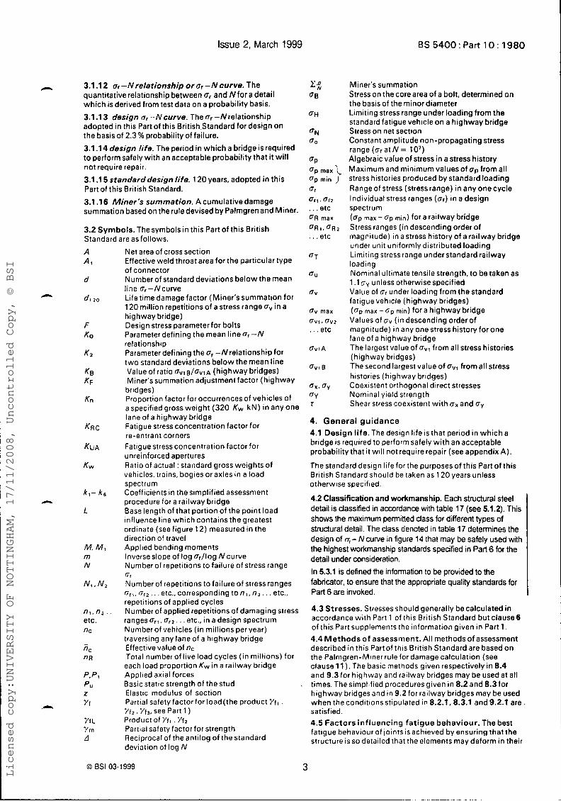
- 3.1.1 2 Qr -N relationship or Or - N curve. The quantitative relationship between Or and Nfo r a detail which is derived from test data on a probability basis.
3.1 -13 design ITr-Ncurve. The Or-Nrelationship adopted in this Part of this British,Standard for design on the basis of 2.3 % probability of failure.
3.1.14 design life. The period in which a bridge isrequired to perform safely with an acceptable probability that it will not require repair.
3.1.1 5 standard design life. 120 years, adopted in this Part of this British Standard.
3.1.1 6 Miner's summation. A cumulative damage summation based on the rule devised by Palmgren and Miner.
3.2 Symbols. Thesymbols in this Part of this British Standard are as follows.
A A1
d
di 2 0 n
KR C
KUA
K w
ki- ka
L n
n , . n , . etc. f l c
f l C -
nR
P.P, P"
Yf
YfL Ym d
Z
n
Net area of cross section Effective weld throat area for the particular type of connector Number of standard deviations below the mean line gr-Ncurve Life time damage factor (Miner's summation for 120 million repetitions of a stress range 0, in a highway bridge) Design stress parameter for bolts Parameter defining the mean line 'Jr -N relationship Parameter defining the ur -N relationship for two standard deviations below the mean line Value of ratio avl B / ~ V ~ A (highway bridges) Miner's summation adjustment factor (highway bridges) Proportion factor for occurrences of vehicles of a specified gross weight (320 Kw kN) in any one lane of a highway bridge Fatigue stress concentration factor for re-entrant corners Fatigue stress concentration factor for unreinforced apertures Ratio of actual : standard gross weights of vehicles, trains, bogies or axles in a load spectrum Coefficients in the simplified assessment procedure for a railway bridge Bass length of that portion of the point load influence line which contains the greatest ordinate (see figure 12) measured in the direction of travel Applied bending moments lnverseslope of log *,/log Ncurve Number of repetitions to failure of stress range 01
Number of repetitions to failure of stress ranges Ori , C r 2 . . . etc., corresponding ton,, n 2 . . . etc., repetitions of applied cycles Number of applied repetitions of damaging stress ranges Or,. U r 2 . . . etc., in a design spectrum Number of vehicles ( in millions per year) traversing any lane of a highway bridge Effective value of nc Total number of live load cycles (in millions) for each load proportion Kw in a railway bridge Amlied ax ia l forces
N
0 0
UH
UN Qo
QP u p max l, Qp min j 'Jr
Q r i , Or2 , . . etc 'JR max
*R 1,'JR2
. . . etc
*T
OU
b V
QV max a v l , av2 . . . etc
'JviA
u v i B
Qx. Qy
*Y r
Miner's summation Stress on the core area of a bolt, determined on the basis of the minor diameter Limiting stress range under loading from the standard fatigue vehicle on a highway bridge Stress on net section Constant amplitude non-propagating stress range(oratN= 10') Algebraic value of stress in a stress history Maximum and minimum values of oP from all stress histories produced by standard loading Range of stress (stress range) in any one cycle Individual stress ranges (ar) in a design spectrum ((ip max - GP min) for a railway bridge Stress ranges (in descending order of magnitude) in a stress history of a railway bridge under unit uniformlydistributed loading Limiting stress range under standard railway loading Nominal ultimate tensile strength, to be taken as 1.1 G~ unless otherwise specified Value of Gr under loading from the standard fatigue vehicle (highway bridges) (0, max - GP min) for a highway bridge Values of G" (in descending order of magnitude) in any one stress history for one lane of a highway bridge The largest value of gvl from all stress histories (highway bridges) The second largest value of ov, from all stress histories (highway bridges) Coexistent orthogonal direct stresses Nominal yield strength Shear stress coexistent with ox and CJ,,
4. Genera l gu idance 4.1 Design l i fe. The design life is that period in which a hridge is required to perform safely with an acceptable probability that it will not require repair (see appendix A).
The standard design life for the purposes of this Part of this British Standard should be taken as 120 years unless otherwise specified.
4.2 Classification and workmanship. Each structural steel detail is dassified in accordance with table 17 (see 5.1.2). This shows the maximum permitted dass for different types of structural detail. The class denoted in table 17 determines the design of U,- N cutve in figure 14 that may be safely used with the highest Workmanship standards specified in Part 6 for the detail under consideration.
In 5.3.1 is defined the information to be provided to the fabricator, to ensure that the appropriate quality standards for Part 6 are invoked.
4.3 Stresses. Stresses should generally be calculated in accordance with Part 1 of this British Standard but clause6 of this Part supplements the information given in Part 1 . 4.4 Methods o f assessment. All methods of assessment described in this Part of this British Standard are based on the Palmgren-Miner rule for damage calculation (see clause 11 ). The basic methods given respectively in 8.4 and 9.3for hiahwav and railwav bridaes mav be used at a l l . "
Basic static strength of the stud Elastic modulus of section Partial safety factor for load(the product Y f , . Yr,. Y f 3 , see Part 1 )
. times. The simplified procedures given in 8.2and 8.3 for highway bridges and in 9.2 for railway bridges may be used when the conditions stipulated in 8.2.1,8.3.1 and 9.2.1 are . satisfied. - -
Product of 71, . Yf2 Partial safety factor for strength Reciprocal of the antilog of the standard deviation of log N
4.5 Factors inf luencing fat igue behaviour. The best fatigue behaviour of joints is achieved by ensuring that the structure is so detailed that the elements may deform in their
Q BSI 03-1999 3
Licensed copy:UNIVERSITY OF NOTTINGHAM, 17/11/2008, Uncontrolled Copy, © BSI
BS 5400: Part 10: 1980
intended ways without introducing secondary deformations and stresses due to local restraints. Stresses may also be reduced, and hence fatigue life increased, by increased thickness of parent metal or weld metal. The best joint performance is achieved by avoiding joint eccenbiaty and welds near free edges and by other controls over the quality of the joints. Performance is adversely affected by concentrations of stress at holes, openings and reentrant corners. Guidance in these aspects is given in table 17 and appendix H. The effect of residual stresses is taken into I account in the classification tables.
5. C lass i f i ca t ion of de ta i l s 5.1. Classif icat ion 5.1 .I General 5.1.1.1 For the purpose of fatigue assessment, each part of a constructional detail subject to fluctuating stress should, where possible, have a particular class designated in accordance with the criteria given in table 17. Otherwise the detail may be dealt with in accordance with 5.2. 5.1 .I .2The classification of each part of a detail depends upon the following :
(a) the direction of the fluctuating stress relative to the detail ; NOTE. Propagation of cracks takes place in a direction perpendicular to the direction of stress. (b) the location of possible crack initiation at the detail ; (c) the geometrical arrangement and proportions of the detail ; (d) the methods and standards of manufacture and inspection.
I
5.1 .I .3 In welded details there are several locations at which potential fatigue cracks may initiate; these are as follows :
(a) in the parent metal of either part joined adjacent to; (1) theendof theweld, (2) a weld toe, (3) a change of direction of the weld,
(b) in the throat of the weld. In the case of members or elements connected at their ends by fillet welds or partial penetration butt welds and flanges with shear connectors, the crack initiation may occur either in the parent metals or in the weld throat : both possibilities should be checked by taking into account the appropriate classification and stress range. For other details, the classifications given in table 17 cover crack initiation at any possible location in the detail. Notes on the potential modes of failure for each detail are given in appendix H.
5.1.2 Classification of detailsin table 17 5.1 -2.1 Table 17 isdivided into three parts which correspond to the three basic types into which details may be classified. These are as follows :
(a) type 1, non-welded details, table 17 (a) ; (b) type 2, welded details on surface, table 17 (b) : (c) type 3, welded details at end connections of members, table 17 (c).
5.1.2.2 Each classified detail is illustrated and given a type number. Table 17 also gives variousassociated criteria and the diagrams illustrate the geometrical features and potential crack locations which determine the class of each detail and are intended to assist with initial selection of the appropriate type number. (For important features that change significantly from one type to another see the footnote to table 17.)
5.1.2.3 A detail should only be designated a particular classification if i t complies in every respect with the tabulated criteria appropriate to i ts type number.
Issue 2, March 1999
5.1.2.4 Class A is generally inappropriate for bridge work and the speaal inspection standards relevant to classes B and C cannot normally be achieved in the vicinrty of welds in bridge work. (For these and other classifications that should be used only when speaal workmanship is specified see the footnote to table 17.)
5.1.2.5 The classifications of table 17 are valid for the qualities of steel products and welds which meet the requirements of Part 6. except where otherwise noted. For certain details the maximum permitted class depends on acceptance criteria given in Part 6.
5.2 Unclassif ied detai ls 5.2.1 General. Details not fully covered in table 17 should be treated as class G, or class W for load carrying weld metal, unless a superior resistance to fatigue is proved by special tests. Such tests should be sufficiently extensive to allow the design or -Ncurve to be determined in the manner used for the standard classes (see appendix A). 5.2.2 Post-welding treatments. Where the classification of table 17 does not give adequate fatigue resistance, the performance of weld details may be improved by post-welding treatments such as controlled machining, grinding or peening. When this is required the detail should be classified by tests as given in 5.2.1. 5.3 Workmanship and inspection
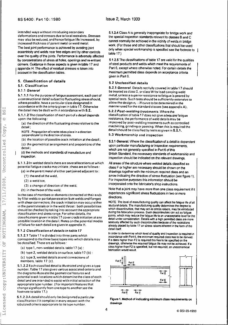
5.3.1 General. Where the classification of a detail is dependent upon particular manufacturing or inspection requirements, which are not generally specified in Part 6 of this British Standard, the necessary standards of workmanship and inspection should be indicated on the relevant drawings.
All areas of the structure where welded details classified as dass F or higher are necessary should be shown on the drawings together with the minimum required class and an arrow indicating the direction of stress fluctuation (see figure 1). For inspection purposes this information should be incorporated onto the fabricator's shop instructions. Note that a joint may have more than one class requirement if it experiences significant stress fluctuations in two or more directions. NOTE. The level of manufacturing quality can affect the fatigue life of all stuctural details. The manufacturing quality determines the degree to which discontinuities, that may act as stress raisers, may be introduced during the fabrication process. Such discontinuities can act as fatigue points, which may reduce the fatigue life to an unacceptable level for the detail under consideration. Details with a high permitted dass are more seriously affected by such discontinuities because of the restrictions already placed by table 17 on stress raisers inherent in the form of the detail itself. In order to dertermine which level of quality and inspection is required in accordance with Part 6, the minimum required dass has to be derived. If a class higher than F2 is required this has to be speafied on the drawings, otherwise the required fatigue life may not be achieved. If a dass higher than F2 is specified, but not required, an uneconomical fabrication would result. E Fat
c ) f )
Fat Fat E
Figure 1. Method of indicating minimum class requirements on drawings
0 BSI 03-1999 4
Licensed copy:UNIVERSITY OF NOTTINGHAM, 17/11/2008, Uncontrolled Copy, © BSI
5.3.2 Detrimenta/ effects. The following occurrences can result in a detail exhibiting a lower performance than its classification would indicate :
(a) weld spatter; (b) accidental arc strikes; (c) unauthorized attachments; (d) corrosion pitting.
5.4 Steel decks. The classifications given in table 17 should not be applied to welded joints in orthotropic steel decks of highway bridges ; complex stress patterns usually occur in such situations and specialist advice should be sought for identifying the stress range and joint classification.
6. Stress calculations 6.1 General 6.1.1 Stress range for welded details. The stress range in a plate or element to be used for fatigue assessment is the greatest algebraic difference between principal stresses occurring on principal planes not more than 45" apart in any one stress cycle. 6.1.2 Stress range for welds. The stress range in a weld is the algebraic or vector difference between the greatest and least vector sum of stresses in any one stress cycle. 6.1.3 Effective stress range for non- welded details For non-welded details, where the stress range is entirely in the compression zone, the effects of fatigue loading may be ignored. For non-welded details subject to stress reversals, the stress range should be determined as in 6.1 .l. The effective stress range to be used in the fatigue assessment should be obtained by adding 60 % of the range from zero stress to maximum compressive stress to that part of the range from zero stress to maximum tensile stress.
-
I
6.1.4 Calculation of stresses 6.1.4.1 Stresses should be calculated in accordance with Part 1 of this British Standard using elastic theory and taking account of a l l axial, bending and shearing stresses occurring under the design loadingsgiven in clause 7. N O redistribution of loads or stresses, such as isallowed for checking static strength at ultimate limit state or for plastic design procedures, should be made. For stresses in
0 BSI 03-1999 4a
Licensed copy:UNIVERSITY OF NOTTINGHAM, 17/11/2008, Uncontrolled Copy, © BSI
Issue 2, March 1999 BS 5400: Part 10: 1980
n composite beams the modulus of elasticity of the concrete should be derived from the short term stress/strain relationship (see Part 4). The stressesso calculated should be used with a material factor Y m = 1. 6.1.4.2 The bending stresses in various parts of a Steel orthotropic bridge deck may be significantly reduced as the result of composite action with the road surfacing. However, thiseffect should only be taken intoaccount On the evidence of special tests or specialist advice. 6.1.5 Effects to be included. Where appropriate, the effects of the following should be included in stress calculations :
(a) shear lag, restrained torsion and distortion, transverse stresses and flange curvature (see Parts 3 and 5 ) ; (b) effective width of steel plates (see Part3) ; (c) cracking of concrete in compositeelements (see Part 5 ) ; (d) stresses in triangulated skeletal structures due to load applications away from joints, member eccentricities at joints and rigidity of joints (see Part 3).
6.1.6 Effects to be ignored. The effects of the following need not be included in stress calculations : -
(a) residual stresses; (b) eccentricities necessarilyarising in a standard detail ; (c) stress concentrations, except as required by table 17 ; (d) plate buckling.
6.2 Stress in parent meta l
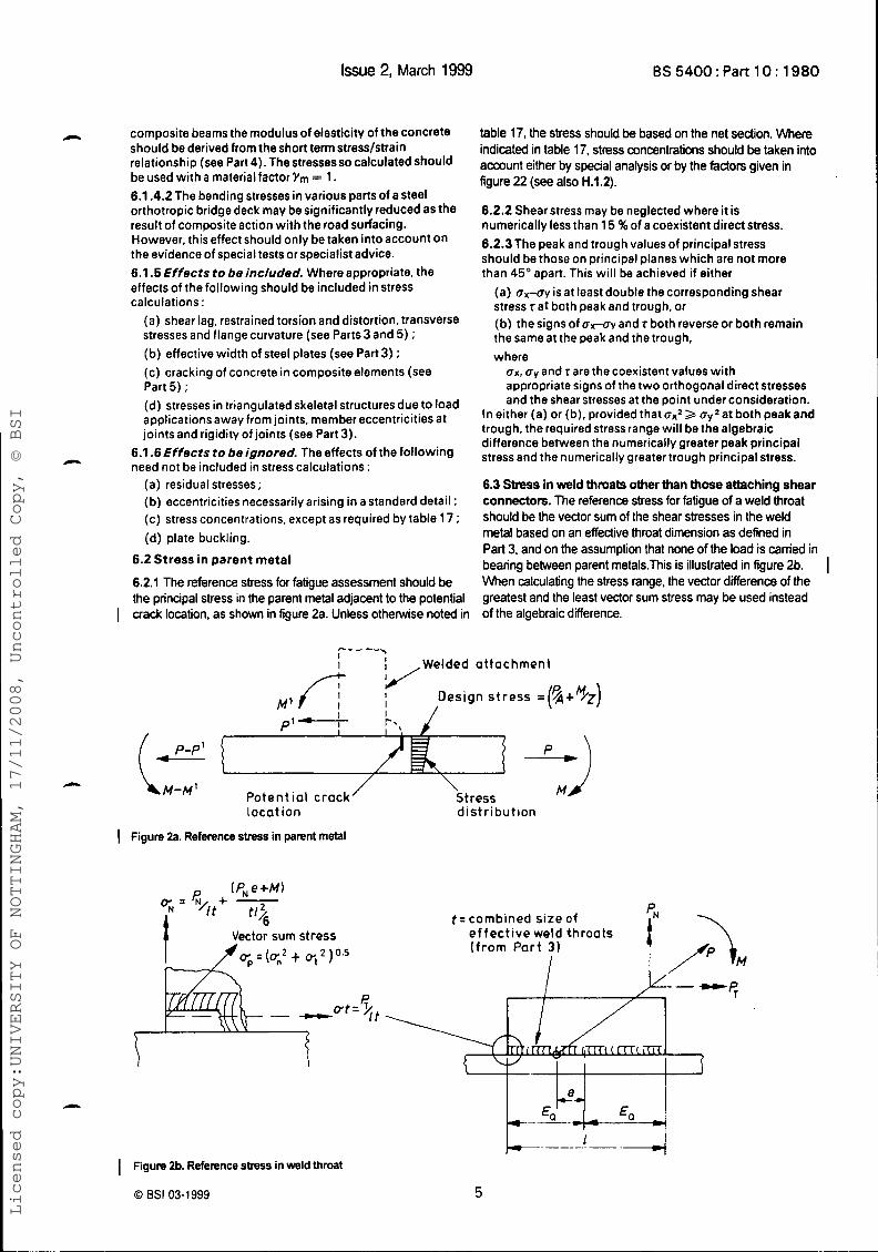
6.2.1 The reference stress for fatigue assessment should be the principal stress in the parent metal adjacent to the potential
table 17, the stress should be based on the net section. Where indicated in table 17. stress concentrations should be taken into account either by special analysis or by the fadors given in figure 22 (see also H.1.2).
6.2.2 Shear stress may be neglected where it is numerically less than 15 %of a coexistent direct stress. 6.2.3 The peak and trough values of principal stress should be those on principal planes which are not more than 45" apart. This will be achieved if either
(a) oX-oy is at least double the corresponding shear stress r a t both peak and trough, or (b) the signs of oX-oy and r both reverse or both remain the sameat the peak and the trough, where
UX, by and r are the coexistent values with appropriate signs of the two orthogonal direct stresses and the shear stresses at the point under consideration.
In either (a) or (b), provided that ox2 2 cq2at both peak and trough, the required stress range will be the algebraic difference between the numerically greater peak principal stress and the numerically greater trough principal stress.
6.3 Stress in weld throats other than those attaching shear connecton. The reference stress for fatigue of a weld throat should be the vector sum of the shear stresses in the weld metal based on an effective throat dimension as defined in Part 3, and on the assumption that none of the load is carried in bearing b e h n parent metals.This is illustrated in figure 2b. When calculating the stress range, the vector difference of the greatest and the least vector sum stress may be used instead
I
I aack location, as shown in figure 2a. Unless otherwise noted in of the algebraic difference
I -"> I i ,Welded a t tachment cc- 4
Design s t r e s s =(/A+ P M /z) M'
\ Stress L M-M' Poten t ia l crack / -
Location d i s t r i bu t i on
I Figure 2a. Reference stress in parent metal
[ P,, e + M 1
Vector sum stress
I Figure Zb. Reference stress in weld throat
0 BSI 03-1999
t = combined size of e f f e c t i v e weld throats ( f r o m Par t 3 )
5
Licensed copy:UNIVERSITY OF NOTTINGHAM, 17/11/2008, Uncontrolled Copy, © BSI
BS 5400:Part 10: 1980
6.4 Stresses in we lds at taching shear connectors 6.4.1 General. For shear connectors in accordance with the dimensional recommendations of Part 5, the design stresses for fatigue in the weld metal should be calculated in accordance with 6.4.2 and 6.4.3. Where thedimensions of the shear connectors and/or the concrete haunches are not in accordance with Part 5, the fatigue strength should be determined in accordance with appendix G of this Part. 6.4.2 Studconnectors. The stresses in the weld metal attaching stud shear connectors should be calculated from the following expression :
stress in weld =
longitudinal shear load on stud appropriate nominalstatic strength (from Part 5) 6.4.3 Channelandbar connectors 6.4.3.1 The stresses in the weld metal attaching channel and bar shear connectors should be calculated from the effective throat area of weld, transverse to the shear flow, when the concrete is of normal density and from 0.85 x throat area when lightweight concrete is used. For the purposes of this clause the throat area should be based on a weld leg length which is the least of the dimensions tabulated below.
x 425Nlmm’
Channel connector Bar connector
of bar) half the thickness of Half the thickness of
beam flange beam flange
6.4.3.2 It may assist calculation to note that in normal density concrete, where the thickness of the beam flange is at least twice the actual weld leg length and the weld dimensions comply with Part 5, the effective weld areas are :
50 x 40 bar connectors i: 200 mm long, 1697 mm 25 x 25 bar connectors :, 200 mrn long, 101 8 rnm’ 127 and 102 channel connectors 150 mm long. 1212 mm2 76 channel connectors ;< 150 mm long, 1081 mm
6.5 Axial stress in bolts. The design stress for fatigue in bolts complying with the requirements of 6s 4395 and bolts to dimensional tolerances complying with the requirements of 6s 3692 should be calculated from the following expression :
F u u
stress in bolt =-= - / uB
F = 1,7kN/mm 2forthreadsof nominaldiarneterupto25mm
F= 2.1 kN/mm2forthreadsof nominaldiameterover25 mm b g is the stress range on the core area of the bolt determined on the basis of the minor diameter ou is the nominal ultimate tensile strength of the bolt material in kN/mm2
where
or
When subjected to fluctuating stresses, black bolts complying with the requirements ot 6s 41 90 may only be used i f they are faced under the head and turned on shank in accordance with the requirements of B S 41 90.
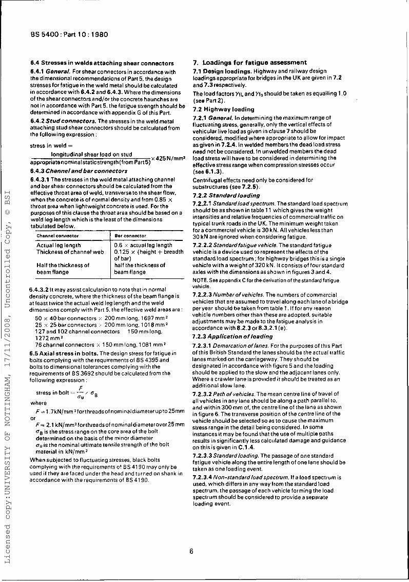
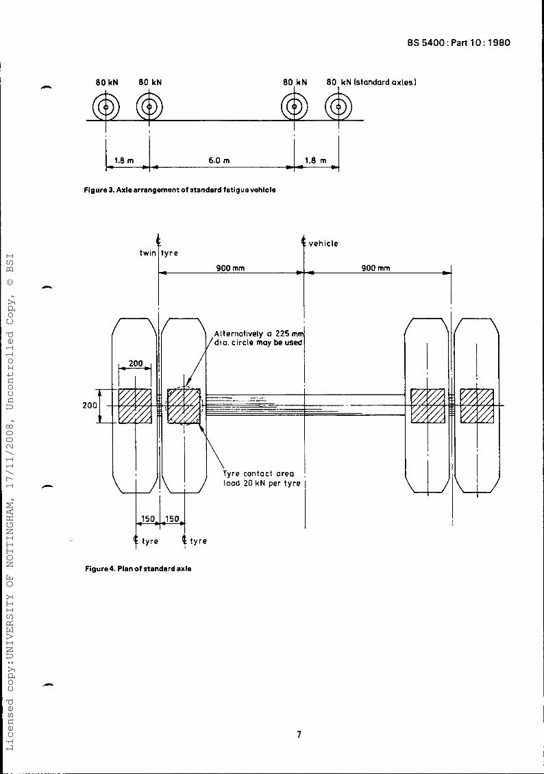
7. Loadings for fatigue assessment 7.1 Design loadings. Highway and railway design loadingsappropriatefor bridges in the UK are given in 7.2 and 7.3 respectively. The load factors YfL and Y f 3 should be taken as equalling 1 .O (see Part2). 7.2 Highway loading 7.2.1 General. In determining the maximum range of fluctuating stress, generally, only the vertical effects of vehicular live load as given in clause 7 should be considered, modified where appropriate to allow for impact as given in 7.2.4. In welded members the dead load stress need not be considered. In unwelded members the dead load stress will have to be considered in determining the effective stress range when compression stresses occur (see6.1.3). Centrifugal effects need only be considered for substructures (see 7.2.5). 7.2.2 Standard loading 7.2.2.1 Standardloadspectrum. The standard load spectrum should beasshown intable 11 whichgivesthe weight intensities and relative frequencies of commercial traffic on typical trunk roads in the UK. The minimum weight taken for a commercial vehicle is 30 kN. All vehicles less than 30 kN are ignored when considering fatigue. 7.2.2.2 Standardfatigue vehicle. The standard fatigue vehicle is a device used to represent the effects of the standard load spectrum ;for highway bridges this is a single vehicle with a weight of 320 kN. It consists of four standard axles with the dimensions as shown in figures 3 and 4. NOTE. See appendix C for the derivation of the standard fatigue vehicle. 7.2.2.3 Number of vehicles. The numbers of commarcial vehicles that are assumed to travel along eachlaneofa bridge per year should be taken from table 1. If for any reason vehicle numbers other than these are adopted, suitable adjustments may be made to the fatigue analysis in accordance with 8.2.3 or 8.3.2.1 (e). 7.2.3 Application of loading
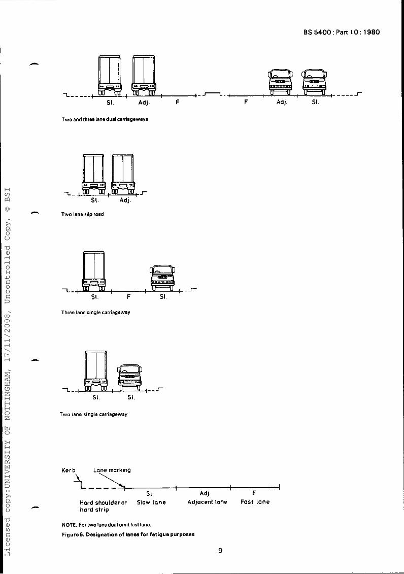
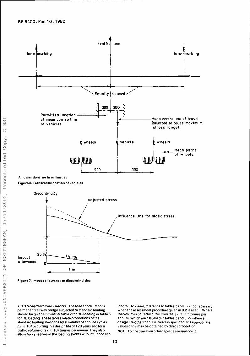
7.2.3.1 Demarcation oflanes. For the purposes of this Part of this British Standard the lanes should be the actual traffic lanes marked on the carriageway. They should be designated in accordance with figure 5 and the loading should be applied to the slow and the adjacent lanes only. Where a crawler lane is provided i t should be treated as an additional slow lane. 7.2.3.2 Path of vehicles. The mean centre line of travel of all vehicles in any lane should be along a path parallel to, and within 300 mm of, the centre line of the lane as shown in figure 6. The transverse position of the centre line of the vehicle should be selected so as to cause the maximum stress range in the detail being considered. In some instances it may be found that the use of multiple paths results in significantly less calculated damage and guidance on this is given in C.1.4. 7.2.3.3 Standardloading. The passage of one standard fatigue vehicle along the entire length of one lane should be taken as one loading event. 7.2.3.4 Non-standardloadspectrum. If a load spectrum is used, which differs in any way from the standard load spectrum, the passage of each vehicle forming the load spectrum should be considered to provide a separate loading event.
6
Licensed copy:UNIVERSITY OF NOTTINGHAM, 17/11/2008, Uncontrolled Copy, © BSI
BS 5400 : Part 10 : 1980
1.8 m -
80kN 80 kN 80, kN 80. kN (standard axles 1
6.0 m 1.8 m t - - - -4
Figure 3. Axle arrangement of standard fatigue vehicle
twin \ tyre
Alternatively a 225 mn dia. circle may be used
Tyre contact area load 20 kN per tyre
vehicle
+ t y r e + t y r e
Figure 4. Plan of standard axle
7
Licensed copy:UNIVERSITY OF NOTTINGHAM, 17/11/2008, Uncontrolled Copy, © BSI
BS5400:Part10:1980
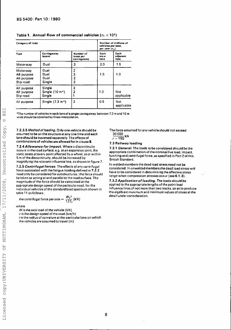
Table 1. Annual flow of commercial vehicles (n, x 1 06)
Motorway
Motorway All purpose All purpose Sfio road
Category of road
Dual 3 2.0 1.5
Dual 2 Dual 3 1.5 1 .o Dual 2 Sinale 2
Number of millions of vehicles per lane, I per year ( n e )
All purpose All purpose
Slip road
Carriageway layout I
Single (10 m* ) Single
Single
Number of Each Each lanes per I carriaaewav
All purpose Single (7.3 m * ) 2 0.5 Not applicable
1 1.0 I Not applicable
7.2.3.5 Methodof loading. Only one vehicle should be assumed to be on the structure at any one time and each lane should be traversed separately. The effects of combinations of vehicles are allowed for in clause 8. 7.2.4 Allowance for impact. Where a discontinuity occurs in the road surface, e.g. at an expansion joint, the static stress at every point affected by a wheel, at or within 5 m of the discontinuity, should be increased by magnifying the relevant influence line, as shown in figure 7. 7.2.5 Centrifugal forces. The effects of any centrifugal force associated with the fatigue loading defined in 7.2.2 need only be considered for substructures; the force should be taken as acting at and parallel to the road surface. The magnitude of the force should be calculated at the appropriate design speed of the particular road, for the individual vehicles of the standard load spectrum shown in table 1 1 as follows :
WY2 127,
the centrifugal force per axle = - (kN)
The force assumed for any vehicle should not exceed 30 000 kN r - 1 5 0
7.3 Rai lway loading 7.3.1 General. The loads to be considered should be the appropriate combination of the nominal live load, impact, lurching and centrifugal force, as specified in Part 2 of this British Standard. In welded members the dead load stress need not be considered. In unwelded membersthedead load stress will have to be considered in determining the effective stress range when compression stresses occur (see 6.1.3). 7.3.2 Application of loading. The loads should be epplied to the appropriate lengths of the point load influence lines of not more than two tracks, so as to produce the algebraic maximum and minimum values of stress at the detail under consideration.
where Wis theaxle load of thevehicle (kN) vis the design speed of the road (km/h) r is the radius of curvature at the particular lane on which the vehicles are assumed to travel (m)
8
Licensed copy:UNIVERSITY OF NOTTINGHAM, 17/11/2008, Uncontrolled Copy, © BSI
SI. Adj. F F Adj. SI.
Two and three lane dual carriageways
n
c
SI. ' Adj.
Two lane slip road
1
SI. ' F SI.
Three lane single carriageway
-L -- --I- SI. SI.
Two lane single carriageway
Lane marking
I 1 1 1 1
SI . Adj. F Hard shoulder or Slow lane Adjacent lane Fast lane hard strip
NOTE. For two lane dual omit fast lane.
Figure S. Designation of lanes for fatigue purposes
9 Licensed copy:UNIVERSITY OF NOTTINGHAM, 17/11/2008, Uncontrolled Copy, © BSI
BS 5400 : Part 10 : 1980
I I
I
All dimensions are in millimetres
Figure& Transverse location of vehicles
t r a f f i c lane 1 Mean centre line of t rave l
Permit ted loca t ion ~A:*L3 of mean cen t re l ine of vehicles
4 wheels
I 4 vehicle
(selected t o cause m a x i m u m s t ress range)
wheels c -Mean po t hs
o f whee ls
900 900
Di scont inuit y
4 Adjusted stress /
Figure 7. Impact allowance at discontinuities
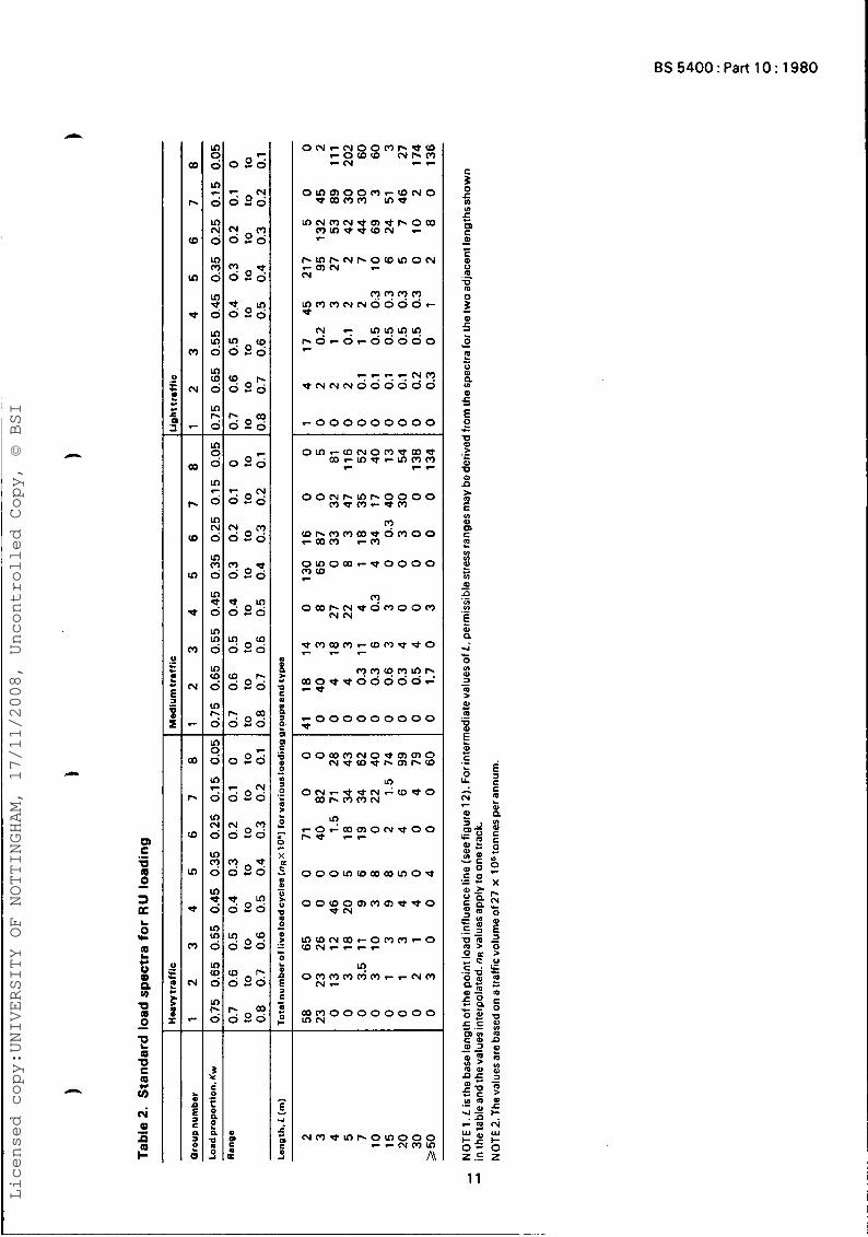
7.3.3 Standard/oad spectra. The load spectrum for a permanent railway bridge subjected to standard loading should be taken from either table 2 for RU loading or table 3 for RL loading. These tables relate proportions of the standard loading Kw to the total number of applied cycles nR x 1 0 6 occurring in a design life of 120 years and for a traffic volume of 27 x 106 tonnes per annum. They also allow for variations in the loading events with influence line
length. However, reference to tables 2 and 3 is not necessary when theassessment procedure given in 9.2 is used. Where the volumes of traftic differ from the 27 Y 1 O6 tonnes per annum, which are assumed in tables 2 and 3, or where a design life other than 120years is specified, the appropriate values of n~ may be obtained by direct proportion. NOTE. For the derivation of load spectra see appendix E.
I 10 Licensed copy:UNIVERSITY OF NOTTINGHAM, 17/11/2008, Uncontrolled Copy, © BSI
I n
P .- 5
n U m
11
Licensed copy:UNIVERSITY OF NOTTINGHAM, 17/11/2008, Uncontrolled Copy, © BSI
8s 5400: Part 10: 1980
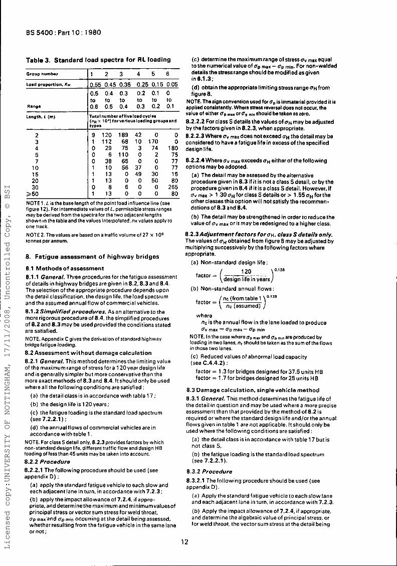
Table 3. Standard load spectra for RL loading
Qroup number
Lord proportion, Kw
Range
Length, 1 (m)
2 3 4 5 7
10 15 20 30
2 5 0
1 2 3 4 5 6
3.55 0.45 0.35 0.25 0.15 0.05 0.5 0.4 0.3 0.2 0.1 0 to to to to to to 3.6 0.5 0.4 0.3 0.2 0.1 rotalnumberof liveloadcycles nR Y 10') forvariousloadinggroupsand yp-
9 120 189 42 0 0 1 112 68 10 170 0 0 29 75 3 74 180 0 6 110 0 2 75 0 38 65 0 0 77 1 10 56 37 0 77 1 13 0 49 30 15 1 13 0 0 50 80 0 8 6 0 0 2 6 5 1 1 3 0 0 0 80
NOTE 1. L is the base length of the point load influence line (see figure 12). For intermediate values of L. permissible stress ranges may be derived from the spectra for the two adjacent lengths shown in the table and the values interpolated. n~ values apply to one track.
NOTE 2. The values are based on a traffic volume of 27 x 1 O6 tonnes per annum.
8. Fatigue assessment of highway bridges
8.1 Methods of assessment 8.1.1 General. Three procedures for the fatigue assessment of details in highway bridges are given in 8.2,8.3 and 8.4. The selection of the appropriate procedure depends upon the detail classification, the design life, the load spectrum and the assumed annual flow of commercial vehicles. 8.1.2 Simplified procedures. As an alternative to the more rigorous procedure of 8.4, the simplified procedures of 8.2 and 8.3 may be used provided the conditions stated are satisfied. NOTE. Appendix C gives the derivation of standard highway bridge fatigue loading. 8.2 Assessment w i t h o u t damage calculat ion 8.2.1 General. This method determines the limiting value of the maximum range of stress for a 120 year design life and is generally simpler but more conservative than the more exact methods of 8.3 and 8.4. It should only be used where all the following conditions are satisfied :
(a) the detail class is in accordance with table 17 ; (b) the design life is 1 20 years ; (c) the fatigue loading is the standard load spectrum (see 7.2.2.1) ; (d) the annual tlows of commercial vehicles are in accordance with table 1 .
NOTE. For class S detail only, 8.2.3 providesfactors by which non-standard design life, different traffic flow and design HB loading of less than 45 units may be taken into account. 8.2.2 Procedure 8.2.2.1 The following procedure should be used (see appendix D) :
(a) apply the standard fatigue vehicle to each slow and each adjacent lane in turn, in accordance with 7.2.3; (b) apply the impact allowance of 7.2.4, i f appro- priate, anddeterminethe maximum and minimumvaluesof principal stress or vector sum stress for weld throat, o p max'and o p min occurring at the detail being assessed, whether resulting from the fatigue vehicle in the same lane or not ;
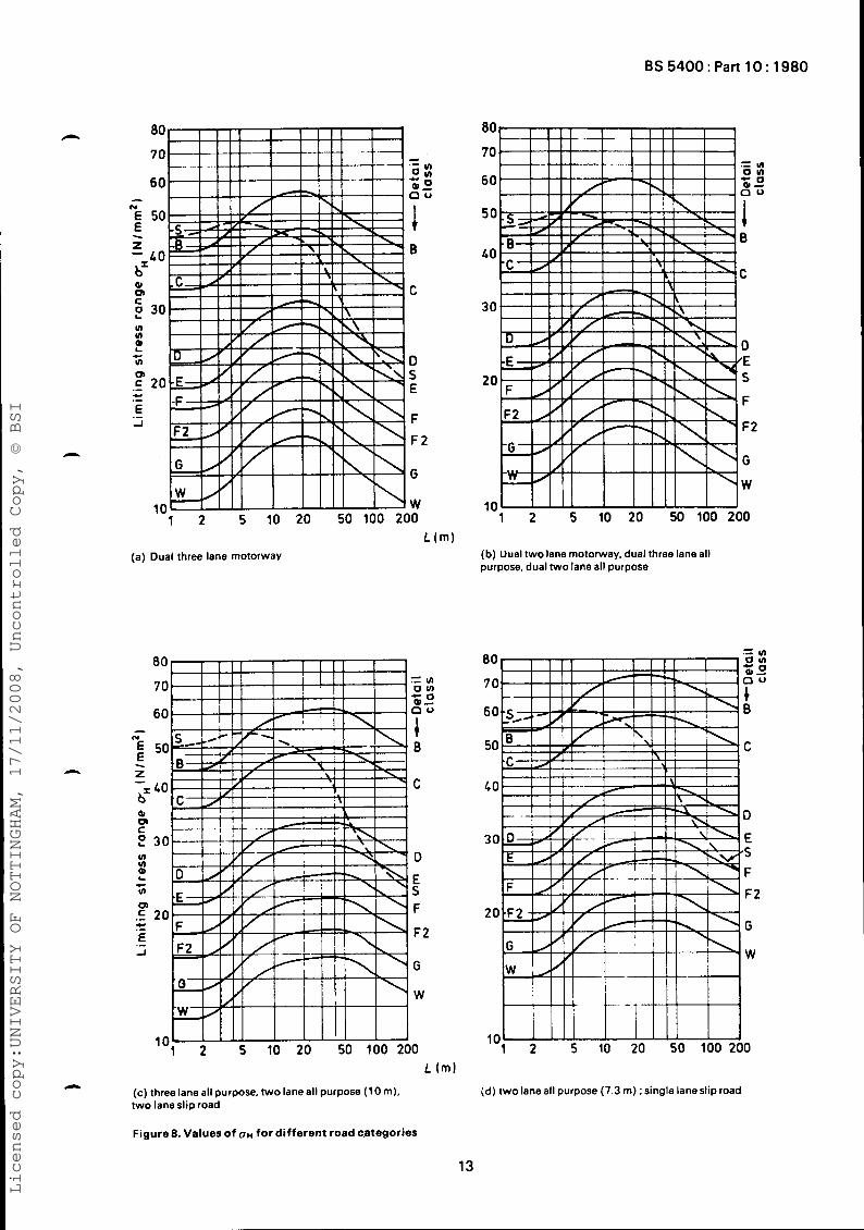
(c) determine the maximum range of stress gV max equal to the numerical value of op max - OP min. For non-welded details the stress range should be modified asgiven in 6.1.3; (d) obtain the appropriate limiting stress range OH from figure 8.
NOTE. The sign convention used for bp is immaterial provided it is applied consistently. Where stress reversal does not occur, the value of either bp
8.2.2.2 For class S details the values of OH may be adjusted by the factors given in 8.2.3, when appropriate. 8.2.2.3 Where ov max does not exceed OH the detail may be considered to have a fatigue life in excess of the specified design life.
8.2.2.4 Where oV max exceeds OH either of the following options may be adopted.
or 0, mln should be taken as zero.
(a) The detail may be assessed by the alternative procedure given in 8.3 if i t is not a class S detail, or by the procedure given in 8.4 if it is a class S detail. However, If ov may > 1.30 OH for class S details or > 1.55 OH for the other classes this option will not satisfy the recommen- dations of 8.3 and 8.4. (b) The detail may be strengthened in order to reduce the value of ov max or it may be redesigned to a higher class.
8.2.3 Adjustment factors foraH. class S details only. The values of OH obtained from figure 8 may be adjusted by multiplying successively by the following factors where appropriate.
(a) Non-standard design life : 0.128
120 . . - ) factor = ( design life in years
(b) Non-standard annual flows :
nc (from table 1 ','*' ( nc (assumed) ) factor =
where nc is the annual flow in the lane loaded to produce Ov max - Op max - b p min
NOTE. In the case where op msx and op ,,,," are produced by loading in two lanes, n, should be taken as the sum of the flows in those two lanes. (c) Reduced values of abnormal load capacity (see C.4.4.2) :
factor = 1.3 for bridges designed for 37.5 units H B factor = 1.7 for bridges designed for 25 units HB
8.3 Damage calculat ion, single vehicle me thod 8.3.1 General. This method determines the fatigue life of the detail in question and may be used where a more precise assessmentthan that provided by the method of 8.2 is required or where the standard design life and/or the annual flows given in table 1 are not applicable. It should only be used where the following conditions are satisfied :
(a) the detail class is in accordance with table 1 7 but is not class S, (b) the fatigue loading is the standard load spectrum (see 7.2.2.1 ) .
8.3.2 Procedure 8.3.2.1 The following procedure should be used (see appendix D).
(a) Apply the standard fatigue vehicle to each slow lane and each adjacent lane in turn, in accordance with 7.2.3. (b) Apply the impact allowance of 7.2.4, if appropriate, and determine the algebraic value of principal stress, or for weld throat, the vector sum stress at the detail being
12
Licensed copy:UNIVERSITY OF NOTTINGHAM, 17/11/2008, Uncontrolled Copy, © BSI
80
70 Ov) z2
60
.= ul
r N E 50 B
bs 40
\ z C -
d, CI, C
30 U) D
S F F2
G
W
U)
E E c ul 0, .E 20
E c .- .- -I
L l m )
(c) three lane all purpose, two lane all purpose (1 0 m), two lane slip road
Figure 8. Values of OH for different road c.ategories
13
80
70
60
50
40
30
20
10 1 2 5 10 20 50 100 200
(b) Uual two lane motorway. dual three lane all purpose, dual two lane all purpose
Licensed copy:UNIVERSITY OF NOTTINGHAM, 17/11/2008, Uncontrolled Copy, © BSI
BS 5400 Part 10: 1980
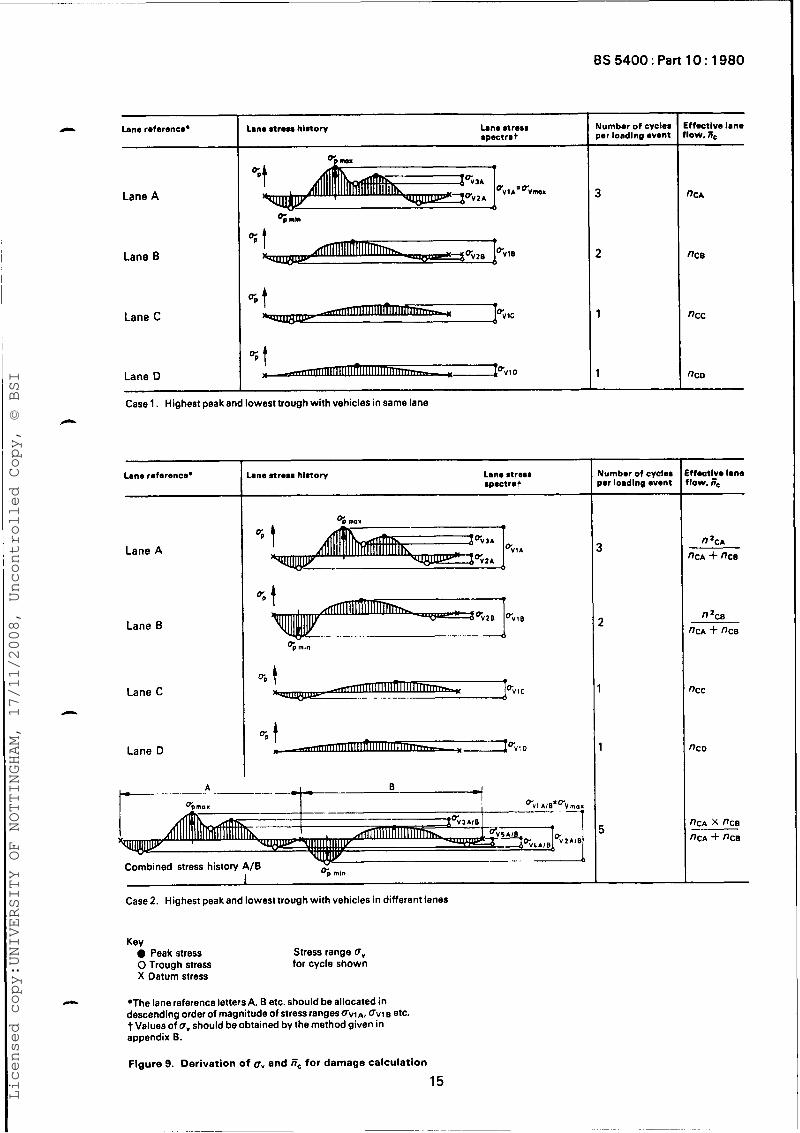
assessed .a each peak and each trough in the stress history of each lane in turn (see figure 9). NOTE. It issufficientlyaccurate tocalculateeach peakor trough value of the direct stress and to obtain the principal stress by combining these with the coincident shear stress, or vice- versa where this is more severe. (c) When the maximum and the minimum algebraic values of stress op max, op min. result from vehicle positionsin thesamelane (referred toascase 1 in figure 9) the damage should be calculated for the stress historiesfor each lane separately. When c ~ p mar and op min result from vehicle positions in different lanes (referred to as case 2 in figure 9) an additional combined stress history should be derived, which allows for the increased maximum stress range produced by a proportion of the vehicles travelling in alternating sequence in the two lanes. In this case the damage should be calculated for the combined stress history as well as for the separate lane stress histories. (d) Derive the stress spectrum ovl, uv2 etc.. from each stress history determined from (c). Where a stress history contains only one peak and/or only one trough, only one cycle results, as shown in figure 9 for lanes C and D, and the stress range can be determined directly. Where a stress history contains two or more peaks and/or two or more troughs, as shown in figure 9 for lanes A and 8 , more than one cycle results and the individual stress ranges should be determined by the reservoir method given in appendix B. (e) Determine the effective annual flow of commercial vehicles, Tic million, appropriate to each stress spectrum as follows :
(1 ) where case 1 of figure 9 applies, & = nc and may be derived directly from table 1 unless different vehicle flows are adopted ; (2) where case 2 of figure 9 applies the effective annual flow fiC should be obtained as indicated in figure 9 for case 2.
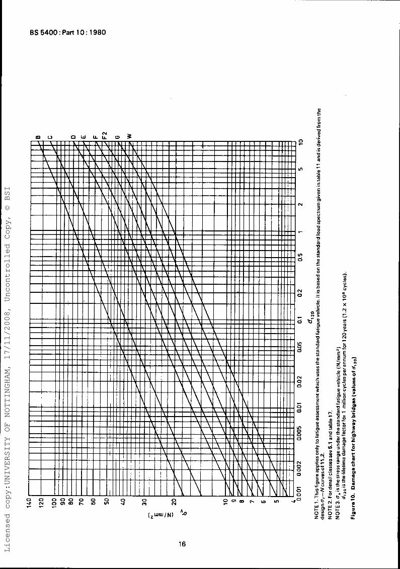
(f) For each stress range ov of each stress spectrum, determine the appropriate lifetime damage factor d, 2o
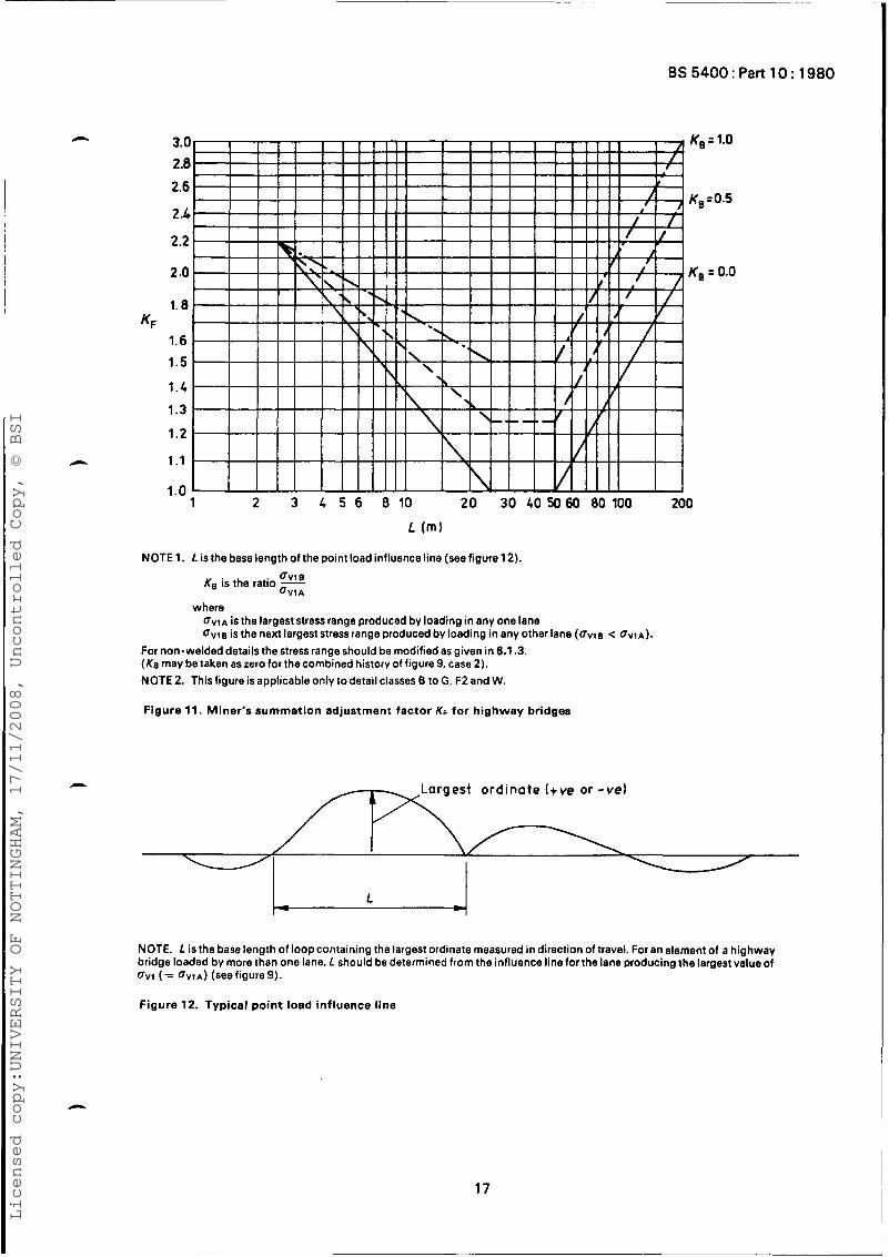
from the damage chart of figure 10 and multiply each of these values by the appropriate value of ifc. For non- welded details the stress range should be modified as in 6.1.3. (g) Determine the value of the adjustment factor KF from figure 11 according to the base length L of the point load influence line (see figure 12) and the stress range ratio KB defined in figure 11. For a combined stress history from two lanes (see (c) above and case 2 in figure 9) KB should be taken as zero for determining K,. NOTE. For the derivation of KF see appendix C. (h) Determine the predicted fatigue life of the detail from the following expression : . .
120 ZKFEcd, 20
fatigue life (in years) =
8.3.2.2 Where the predicted fatigue life of the detail is less than the specified design life, the detail should either be strengthened to reduce the value of uv max or redesigned to a higher class and then re-checked as in 8.3.2.1. As a guide, an approximate stress range for the same class of detail can be obtained by multiplying the original value by :
(predicted life) "(m+O
m is the inverse slope of the appropriate log ar/log N curve given in table 8.
design life where
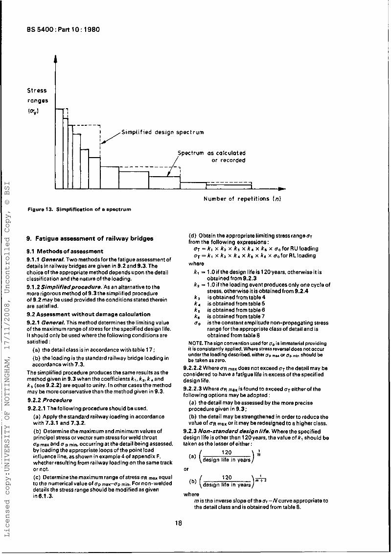
If the detail is to be redesigned to a higher class the procedure given in 11.5( b) may be used as a guide to assess the adequacy of the proposed detail. 8.4 Damage calculation, vehicle spectrum method 8.4.1 General. This method involves an explicit calculation of Miner's summation and may be used for any detail for which the a,-Nrelationship is known and for any known load or stress spectrum. 8.4.2 Design spectrum 8.4.2.1 The individual stress spectra for the detail being assessed should be derived by traversing each vehicle in the load spectrum along the various lanes. Account should also be taken of the possibility of higher stressrangesdue to some of the vehicles occurring simultaneously in one or more lanes and/or in alternating sequence in two lanes. For non-welded details the stress range should be modified as given in 6.1.3. 8.4.2.2 In the absence of other evidence, allowance for impact should be made in accordance with 7.2.4. The design spectrum should then be determined by combining the stress spectra with the specified numbers of vehicles in the respective lanes. 8.4.2.3 In assessing an existing structure, a design spectrum may be compiled from strain readings or traffic records obtained from continuous monitoring. 8.4.3 Simplification of design spectrum. The design spectrum may be divided into any convenient number of intervals, as shown in figure 13, with a l l the stress ranges in any one interval being treated as the maximum range in that interval but low stress ranges should be treated in accordance with 11.3. It should be noted that the use of small intervals will reduce the conservatism in fatigue assessment. 8.4.4 Calculation of d8mege. Using the design spectrum,
the value of Miner'ssummation - should be calculated in
accordance with clause 11. This value should not exceed 1 .O for the fatigue life of the detail to be acceptable.
=I
14
where the summation includes all the separate lane stress histories as well as the combined stress history, where appropriate.
Licensed copy:UNIVERSITY OF NOTTINGHAM, 17/11/2008, Uncontrolled Copy, © BSI
BS 5400 : Part 10: 1980
c I
Lane reference* I Lane a t r o u hinow Lane streas smctrat
Lane A
Lane B
Lane C
I - 1 A .
1c I - p
Lane 0 1
Case 1. Highest peak and lowest trough with vehicles in same lane
~
Lane reference'
Lane A
Lane B
Lane C
Lane D
one n r e u hlnory Lane straso apmctrat
1c
I Pv*rre
I 5 min Combined stress history A/B
I
Case 2. Highest peak and lowest trough withvehicles in different lanes
Stress range Q, for cycle shown
Key 0 Peak stress 0 Trough stress X Datum stress
*The lane reference letters A, B etc. should be allocated in descending order of magnitude of stress ranges OVlA, CJvi 6 etc. t Values of b, should be obtained by the method given in appendix B.
Figure 9. Derivation o f gv and is, for damage calculation
15
Number of cyclea per loedlng *V*nt
dumber of cyclea )er loading event
ffoctlve lane IOW. E,
ffoctlv. Imne low. iic
k c
Licensed copy:UNIVERSITY OF NOTTINGHAM, 17/11/2008, Uncontrolled Copy, © BSI
BS 5400 Part 10: 1980
al 5
VI .- U m
e m
in
I
16
Licensed copy:UNIVERSITY OF NOTTINGHAM, 17/11/2008, Uncontrolled Copy, © BSI
c
BS 5400 : Part 10 :.1980
NOTE 1. L is the base length of the point load influence line (see figure 12). oVl B
U V l A K, is the ratio -
where Q V l A is the largest stress range produced by loading in any one lane ov1B is the nexl largest stress range produced by loading in any other lane ( ~ V C B < oV1A).
For non-welded details the stress range should be modified as given in 6.1.3. (Ke may be taken as zero for the combined history of figure 9, case 2). NOTE 2. This figure is applicable only to detail classes B to G, F2 and W.
Figure 11. Miner's summation adjustment factor KF for highway bridges
- -Largest ordinate ( tve or -vel
NOTE. L is the base length of loop containing the largest ordinate measured in direction of travel. For an element of a highway bridge loaded by more than one lane, L should be determined from the influence line for the lane producing the largest value of bv i (= O V l A ) (seefigure9).
Figure 12. Typical po in t load influence line
17
Licensed copy:UNIVERSITY OF NOTTINGHAM, 17/11/2008, Uncontrolled Copy, © BSI
BS 5400 : Part
Stress
ranges
10; 1
0: 1980
1 I I
__--- ,Simplified design spectrum
Spectrum as calculated or recorded
_--__---
Number of repetit ions ( n )
Figure 13. Slmpliflcstlon of e spectrum
9. Fatigue assessment of railway bridges
9.1 Methods of assessment 9.1.1 Gener81. Two methods for the fatigue assessment of details in railway bridges are given in 9.2 and 9.3. The choice of the appropriate method depends upon the detail classification and the nature of the loading. 9.1.2 Simplifiedprocedure. 'As an alternative to the more rigorous method of 9.3 the simplified procedure of 9.2 may be used provided the conditions stated therein are satisfied. 9.2 Assessment wi thout damage calculation 9.2.1 Gener81. This method determines the limiting value of the maximum range of stress for the specified design life. It should only be used where the following conditions are satisfied :
(a) the detail class is in accordance with table 17 ; (b) the loading is the standard railway bridge loading in accordance with 7.3.
The simplified procedure produces the same results as the method given in 9.3 when the coefficientsk,, k,, k 4 and k 5 (see 9.2.2) are equal to unity. In other cases the method may be more conservative than the method given in 9.3. 9.2.2 Procedure 9.2.2.1 The following procedure should be used.
(a) Apply the standard railway loading in accordance with 7.3.1 and 7.3.2. (b) Determine the maximum and minimum values of principal stress or vector sum stress for weld throat u p max and CJ p min, occurring at the detail being assessed, by loading the appropriate loops of the point load influence line, asshown in example 4of appendix F. whether resulting from railway loading on the same track or not. (c) Determine the maximum range of stress OR max equal to the numerical value of crp max-bp min. For non-welded details the stress range should be modified as given in 6.1.3.
(d) Obtain the appropriate limiting stress range b~ from the following expressions:
UT = k , x k; x k 3 x k , x k s x do for RU loading QT = k l x k2 x k4 x k s x ke x dofor RLloading
k , = 1 .O if the design life is 120 years, otherwise it is
k2 = 1 .O if the loading event produces only one cycle of
kr k 4 k B k s go
where
obtained from 9.2.3
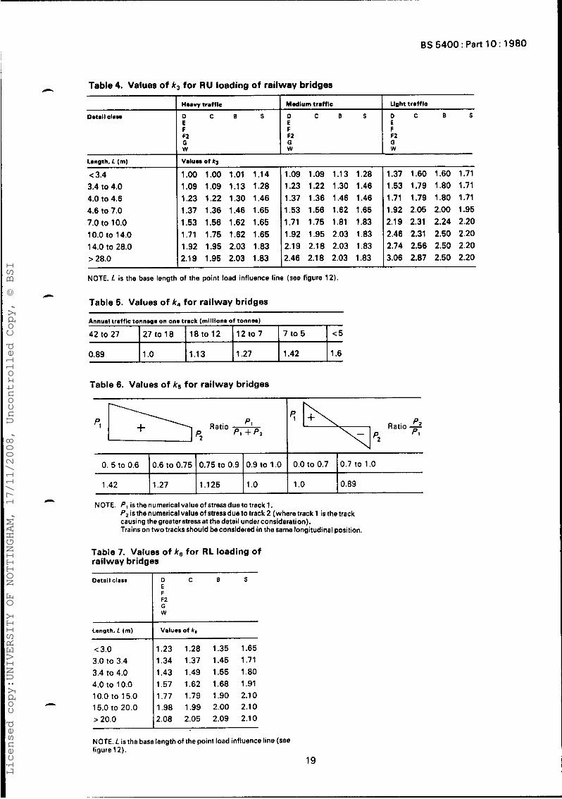
stress, otherwise it is obtained from 9.2.4 is obtained from table 4 is obtained from table 5 is obtained from table 6 is obtained from table 7 is the constant amplitude non-propagating stress range for the appropriate class of detail and is obtained from table 8
NOTE. The sign convention used for bp is immaterial providing it is consistently applied. Where stress reversal does not occur under the loading described, either bp msx or bp ,,,in should be be taken as zero.
9.2.2.2 Where U R max does not exceed UT the detail may be considered to have a fatigue life in excess of the specified design life. 9.2.2.3 Where CYR max is found to exceed GT either of the following options may be adopted :
(a) the detail may be assessed by the more precise procedure given in 9.3; (b) the detail may be strengthened in order to reduce the value of OR max or it may be redesigned to a higher class.
9.2.3 Non-st8nd8rd designlife. Where the specified design life is other than 120 years, the value of k , should be taken as the lesser of either :
(a) (design life 120 in years ) or
120 )A (b) (design life in years
where m is the inverse slope of the br -N curve appropriate to the detail class and is obtained from table 8.
18
Licensed copy:UNIVERSITY OF NOTTINGHAM, 17/11/2008, Uncontrolled Copy, © BSI
BS 5400: Part 10: 1980
Heavy trafflc Mullurn trafflc
E E F F F2 F2 0 0 W W
Detail clem D C 8 S 0 C B S
Llght trafflc
O C E F F2 0 W
8 S
Length. L (m)
< 3.4 3.4 to 4.0 4.0 to 4.6 4.6 to 7.0 7.0 to 10.0 10.0 to 14.0 14.0 to 28.0 > 28.0
Valume of &3
1.00 1.00 1.01 1.14 1.09 1.09 1.13 1.28 1.09 1.09 1.13 1.28 1.23 1.22 1.30 1.46 1.23 1.22 1.30 1.37 1.36 1.46 1.53 1.56 1.62 1.71 1.75 1.62 1.92 1.95 2.03 2.19 1.95 2.03
.46
.65 -65 .65 .83 .83
1.37 1.36 1.46 1.46 1.53 1.56 1.62 1.65 1.71 1.75 1.81 1.83 1.92 1.95 2.03 1.83 2.19 2.18 2.03 1.83 2.46 2.18 2.03 1.83
1 I
NOTE. I! is the base length of the point load influence line (see figure 12).
42 to 27 27to18 18 to12 1 2 t o 7 7 t o 5
0.89 1 .o 1.13 1.27 1.42
- Table 5. Values of k4 for railway bridges
<5
1.6
0. 5 to 0.6 0.6 to 0.75 0.75 to 0.9 0.9 to 1.0
1.42 1.27 1.1 25 1 .o
Table 6. Values of k5 for railway bridges
0.0 to 0.7
1 .o 0.89
0.7 to 1.0
1.37 1.60 1.60 1.71 1.53 1.79 1.80 1.71 1.71 1.79 1.80 1.71 1.92 2.05 2.00 1.95 2.19 2.31 2.24 2.20 2.46 2.31 2.50 2.20 2.74 2.56 2.50 2.20 3.06 2.87 2.50 2.20
Detail class
Length, L (m)
< 3.0 3.0 to 3.4 3.4 to 4.0 4.0 to 10.0 10.0 to 15.0 15.0 to 20.0 > 20.0
c
0 C 8 S E F F2 G W
V ~ I J O S O f ha
1.23 1.28 1.35 1.65 1.34 1.37 1.45 1.71 1.43 1.49 1.55 1.80 1.57 1.62 1.68 1.91 1.77 1.79 1.90 2.10 1.98 1.99 2.00 2.10 2.08 2.05 2.09 2.10
NOTE. P , is the numerical value of stress due to track 1. P, is the numerical value of stress due to track 2 (where track 1 is the track causing the greater stress at the detail under consideration), Trains on two tracks should be considered in the same longitudinal position.
Table 7. Values of ks for RL loading of railway bridges
Licensed copy:UNIVERSITY OF NOTTINGHAM, 17/11/2008, Uncontrolled Copy, © BSI
B S 5 4 0 0 : P a r t l O : 1980
9.2.4 Multiple cycles. Where the loading event produces more than one cycle of stress the value of k2 should be taken as :
m OR2 OR3 ( OR1 OR I
I+(--) +(-) +.... where
rn is defined in 9.2.3 UR I , ORZ. OR 3 etc. are the stress ranges, in descending order of magnitude, at the individual cycles produced by the approach, passage and departure of a unit uniformly distributed load. NOTE. Such cycles should be counted and the individual strew ranges determined by the reservoir method given in appendix 8. An illustration of the multiple cycle stress history is given in example 4 of appendix F.
9.3 Damage calculat ion 9.3.1 General, This method involves a calculation of Miner's summation and may be used for any detail for which the or -N relationship is known and for any known load or stress spectra. It may also be used as a more precise alternative to the simplified procedure of 9.2. 9.3.2 Design spectrum for standard loading 9.3.2.1 Applying the standard railway loading as given in 7.3.1 and 7.3.2 the value of OR max should be derived in accordance with the procedure set out in 9.2.2.1 (a) to (c). The design spectrum should then be determined by the use of either table 2 for RU loading or table 3 for RL loading (amended where appropriate in accordance with 7.3.3). These tables indicate, for simply supported members, the equivalent frequency of occurrence of stress ranges of varying magnitudes resulting from the passage of the individual trains forming various standard traffic types, where the stress ranges are expressed as proportions of the maximum stress range. 9.3.2.2 In the case of loading from more than one track, account should be taken of the possibility of stress fluctuations arising from the passage of trains on not more than two tracks, both separately and in combination. As an approximation, the effects of two track loading may be obtained by dividing OR max (see 9.3.2.1) by the coefficientkS which can beobtained from table 6. 9.3.2.3 Where the approach, passage and departure of a unit uniformly distributed load produces more than one cycle of stress, as for instance in multi-span longitudinal or cross members or in continuous deck slabs, all the cycles should be taken into account. The appropriate standard trains of figure 19 or figure 20 should be traversed across the relevant point load influence lines and the resulting stress histories should be analysed by the reservoir method, given in appendix B, to derive the respective stress spectra. These should then be combined with the appropriate annual occurrences obtained from table 15 or table 16 proportioned for the required traffic volume and multiplied by the specified design life to produce the overall design spectrum. As an approximation, the effect of the additional cycles may be obtained by dividing either UR max (see 9.3.2.1 ) or OR max/ks(see 9.3.2.2) by the coefficientkZ which should be obtained from 9.2.4. 9.3.3 Design spectrum for non-standard loading 9.3.3.1 Where the loading does not comply with 7.3.1 the appropriate train should be traversed across the relevant point load influence lines and the resulting stress histories should be analysed by the rainflow method to derive the
respective stress spectra. These should then be combined with the appropriate total occurrences in the design life of the bridge to compile the overall design spectrum. For non-welded details the stress range should be modified as given in 6.1 3. 9.3.3.2 In assessing an existing structure, a design spectrum may be compiled from strain readings or traff ic records obtained from continuous monitoring. 9.3.4 Simplification of spectrum. Where a non- standard loading is used in accordance with 7.1, or the stress ranges are obtained from strain gauge readings, the design spectrum should be divided into at least 10 equal intervals of stress. All the stress ranges in any one interval should be treated as the mean range in that interval and low stress ranges should be treated in accordance with 11.3. 9.3.5 Calculation of damage. Using the design spectrum, the value ot Miner's surnmat ionZ i should be calculated in accordance with clause 11 and should not exceed 1 .O for the fatigue life of the detail to be acceptable.
10. Fatigue assessment of b r idges carrying highway and r a i l w a y loading In the case of bridges carrying both highway and railway loadings, the total damage (i.e. 120 years divided by the predicted life) should bedetermined for each loading condition separately, in accordance with 8.3 or 8.4 and 9, To obtain the total damage, the sum of the two damage values should be multiplied by a further adjustment factor which takes into account the probability of coexistence of the two types of loading. This factor should be determined for a given member after consideration of the fact that coincidence of highway traffic on multiple lanes and of railway traffic on multiple tracks has already been taken into account in assessing the separate damage values. Except at very busy.railway stations, where the probability of coincidence of rail and road traffic is higher than on the open track, the adjustment factor is not expected to exceed 1.2 where the stressesfrom highway and railway loading are of the same sign.
11. The P a l m g r e n - M i n e r r u l e
11.1 General. Thevalue of Miner'ssummation xi for use in 8.4.4 and 9.3.5 should be determined from the following expression :
f l 2 . . . . . . 2) Nn
where n , , n 2 . . . n, are the specified numbers of repetitions of the various stress ranges in the design spectrum, which occur in the design life of the structure. NOTE. The number of repetitions may be modified in accordance with 11.3, and for non-welded details the stress rangeshould be modified as given in 6.1.3. NI. N2.. . N,, are the corresponding numbers of repetitions to failure for the same stress ranges, obtained from 11.2.
I.
*The rainflow method is described in ORE D128 Report No. 5 'Bending moment spectra and predicted lives of railway bridges'. published by the Office for Research and Experiments of the International Union of Railways. The reservoir method of cyclecounting, described in appendix 6 for highway bridges. may be applied tostress histories for railway bridges (see example 4 of appendix F) and will produce the same results as the rainflow method for many repetitions of the loading event.
20
Licensed copy:UNIVERSITY OF NOTTINGHAM, 17/11/2008, Uncontrolled Copy, © BSI
BS 5400 : Part 10 : 1980
21
Licensed copy:UNIVERSITY OF NOTTINGHAM, 17/11/2008, Uncontrolled Copy, © BSI
BS5400:Par t lO: 1980
W 13.0 G 13.0
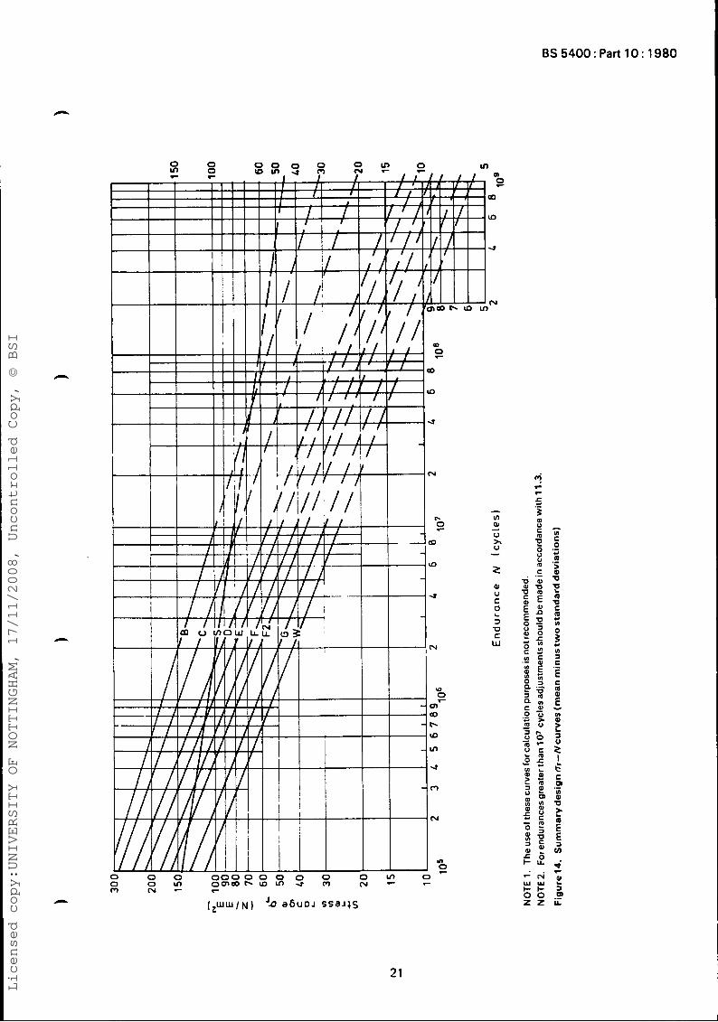
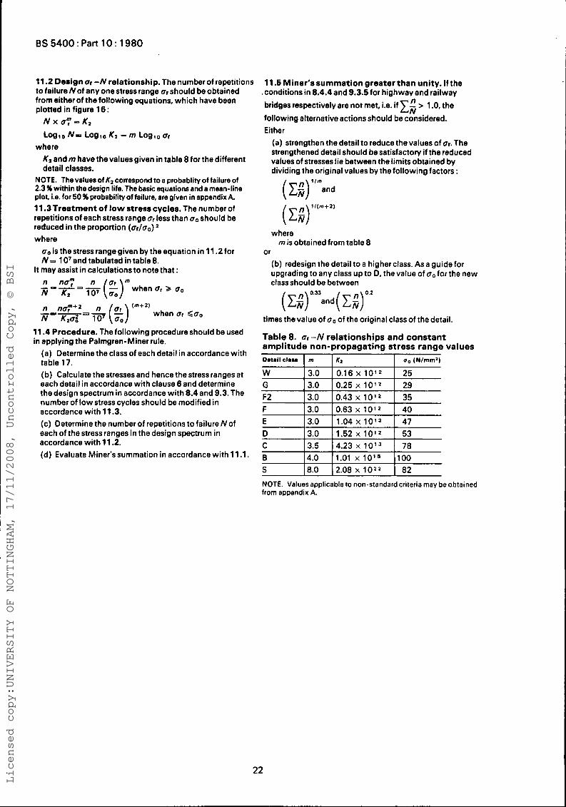
11.2 Design ur -N relationship. The number of repetitions to failure N of any one stress range or should be obtained from either of the following equations, which have been plotted in figure 16 :
N x U': = K, Log,, N = Log10 Kn - m Logqo ur
K2 and m have the values given in table 8 for the different detail classes.
where
NOTE. The valuesof K2 correspond to a probablity of failure of 2.3 %within the design life. The basic equations and a mean-line plot i.e. for 50 %probability of failure, are given in appendix A. 11.3 Treatment of low stress cycles. The number of repetitions of each stress range Or less than U, should be reduced in the proportion (Ur/ao) 2
where U, is the stress range given by the equation in 11.2 for N = 10' and tabulated in table 8.
It may assist in calculations to note that :
0.16 x 10¹² 25 0.25 x 10" 29
11.4 Procedure. The following procedure should be used in applying the Palmgren-Miner rule.
(a) Determine the class of each detail in accordance with table 17. (b) Calculate the stresses and hence the stress ranges at each detail in accordance with clause 6 and determine the design spectrum in accordance with 8.4 and 9.3. The number of low stress cycles should be modified in accordance with 11.3. (c) Determine the number of repetitions to failure N of each of the stress ranges in the design spectrum in accordance with 11.2. (d) Evaluate Miner's summation in accordance with 11 .le
22
11 .S Miner'ssummation greater than unity. If the ,conditions in 8.4.4 and 9.3.5 for highwav and railway bridges respectively are not met, i.e. if 12 > 1 .O, the following alternative actions should be considered. Either
N
(a) strengthen the detail to reduce the values of Or. The strengthened detail should be satisfactory if the reduced values of stresses lie between the limits obtained by dividing the original values by the following factors :
( E;) 'lmand
where m is obtained from table 8
or (b) redesign the detail to a higher class. As a guide for upgrading to any class up to 0, the value of uo for the new class should be between
times the value of uo of the original class of the detail.
Table 8. ur -N re lat ionships and constant ampl i tude non-propagat ing stress range values
F2 13.0 10.43 x 10'2 I 35 F 13.0 10.63 x 10'2 I 40 E 13.0 11 .04~1012 I 47 D (3.0 11 .52~1012 I 53
13.5 14.23 x 10¹³ I 78 C B 14.0 11.01 x l O l s 1100 S 18.0 12.08 x 1 0 2 2 I 82
NOTE. Values applicable to non-standard criteria may be obtained from appendix A.
Licensed copy:UNIVERSITY OF NOTTINGHAM, 17/11/2008, Uncontrolled Copy, © BSI
BS 5400: Part 10: 1980
Appendix A
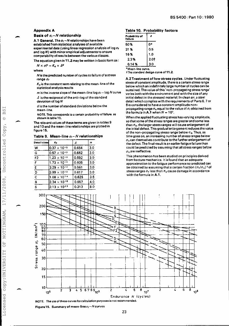
A. l General. The or-N relationships have been established from statistical analyses of available experimental data (using linear regression analysis of log or and log N) with minor empirical adjustments to ensure compatability of results between the various classes. The equation given in 11.2 may be written in basic form as :
where
- Basis of a,-N relationship
N x U?' = K O x Ad
N is the predicted number of cycles to failure of a stress range ur KO is the constant term relating to the mean-line of the statistical analysis results m is the inverse slope of the mean-line log Or -log N curve A is the reciprocal of the anti-log of the standard deviation of log N d is the number of standard deviations below the mean-line. NOTE. This corresponds to a certain probability of failure. as shown in table 10.
The relevant values of these termsare given in tables 9 and 10 and the mean-line relationships are plotted in figure 15.
Table 9. Mean-line or-N relationships
.c
Detril clard KO I d m
W 10.37 x 1 0 1 2 10.654 13.0 10.57 x 10" 10.862 1;::
;2 1.23 x 10 l2 0.592 1.73 x 101 2 0.605 3.0
E 13.29 x 10' I 0.561 13.0 D 13.99 x 1 0 1 2 10.617 13.0 C Il.08 x 1014 10.625 13.5 B 12.34 x 10' I 0.657 14.0 S 12.13 x lOZ3 10.313 18.0
Table 10. Probability factors Probmbllity of Id trlluro
::: ;i 2.3 % 2.0t 0.14%
*Mean-line curve. tThe standard design curve of 11.2.
A.2Treatment of low stress cycles. Under fluctuating stress of constant amplitude, there is a certain stress range below which an indefinitely large number of cycles can be sustained. The value of this'non-propagating stress range' varies both with the environment and with the size of any initial defect in the stressed material. In clean air, a steel detail which complies with the requirements of Parts 6,7 or 8 is considered to have a constant amplitude non- propagating range oo equal to the value of ur obtained from the formula in A.l when N = 1 07. When the applied fluctuating stress has varying amplitude, so that some of the stress ranges are greater and some less than uo, the larger stress ranges wil l cause enlargement of the initial defect. This gradual enlargement reduces the value of the non-propagating stress range below u0. Thus, as time goes on, an increasing number of stress ranges below uo can themselves contribute to the further enlargement of the defect. The final result is an earlier fatigue failure than could be predicted by assuming that all stress ranges below uo are ineffective. This phenomenon has been studied on principles derived from fracture mechanics. It is found that an adequate approximation to the fatigue performance so predicted can be obtained by assuming that a certain fraction (flr/Oo) of stress ranges Q, less than oo cause damage in accordance withtheformula inA.1.
Endurance N (cyc les) NOTE. The use of these curvesfor calculation purposes is not recommended.
Figurel5. Summary of mean-linea,-Ncurves 23
Licensed copy:UNIVERSITY OF NOTTINGHAM, 17/11/2008, Uncontrolled Copy, © BSI
BS 5400:Part 10: 1980
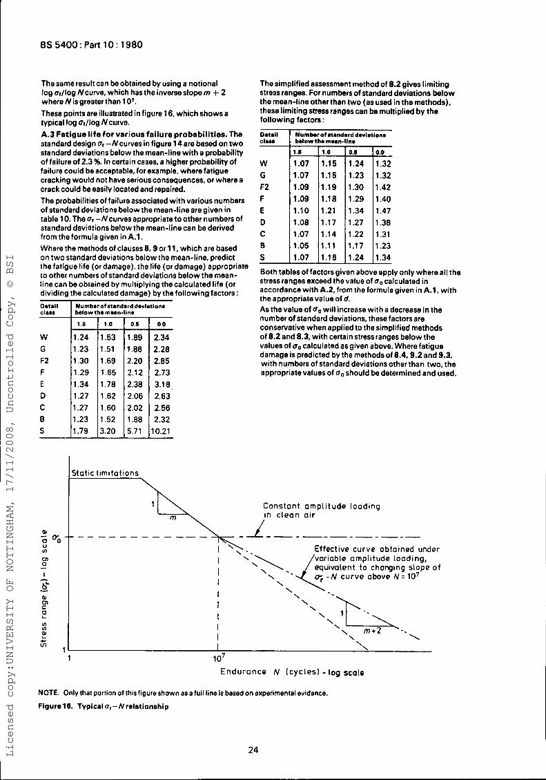
Datal1 c l a r
W G F2 F E D C B S
The same result can be obtained by using a notional log ar/log Ncurve, which has the inverse slope m + 2 where Nisgreaterthanlo’. These points are illustrated in figure 16, which shows a typical log Or/lOg Ncurve. A.3 Fatigue l i fe for various failure probabilities. The standarddesign Qr-Ncurves in figure 14are based on two standard deviations below the mean-line with a probability of failure of 2.3 %. In certain cases, a higher probability of failure could be acceptable, for example, where fatigue cracking would not have serious consequences, or where a crack could be easily located and repaired. The probabilities of failure associated with various numbers of standard deviations below the mean-line are given in table 10. The Qr -Ncurves appropriate to other numbers of standard deviations below the mean-line can be derived from theformula given in A.l. Where the methods of clauses 8.9 or 11, which are based on two standard deviations below the mean-line, predict the fatigue life (or damage), the life (or damage) appropriate to other numbers of standard deviations below the mean- line can be obtained by multiplying the calculated life (or dividing the calculated damage) by the following factors :
Numbmrof atmndard davlatlona balowthamun-llna
1.6 1.0 0.6 0.0
1.07 1.15 1.24 1.32 1.07 1.15 1.23 1.32 1.09 1.19 1.30 1.42 1.09 1.18 1.29 1.40 1.10 1.21 1.34 1.47 1.08 1.17 1.27 1.38 1.07 1.14 1.22 1.31 1.05 1.11 1.17 1.23 1.07 1.16 1.24 1.34
W G F2 F E D C B S
Number of rtandard dOvlatlon8 bSlow1 - 1.5 -
1.24 1.23 1.30 1.29 1.34 1.27 I .27 1.23 I .79
a moan
1 .o - - 1.53 1.51 1.69 1.65 1.78 1.62 1.60 1.52 3.20 -
ne - 0.1 -
1 .89 1.86 2.20 2.1 2 2.38 2.06 2.02 1.88 5.71
- 0.0
2.34 2.28 2.85 2.73 3.18, 2.63 2.56 2.32
10.21
-
itatic limitations
Constant amp1 i tude loading in c lean a i r
Effective curve obtained under variable amplitude loading,
- - - - - - - - - _ - _
I I I \
I \
I I I I \ \
\
\
\ \
\
\ \ m + 2 -.
I 1 o7
\ \
Endurance N (cycles) - log scale
24
NOTE. Only that portion of this figure shown as a full line is based on experimental evidence.
Figure 16. Typical U,-N relationship
Licensed copy:UNIVERSITY OF NOTTINGHAM, 17/11/2008, Uncontrolled Copy, © BSI
BS 5400: Part 10: 1980
Appendix B Cycle counting by the reservoir method 6.1 General. The purpose of cycle counting is to reduce an irregular series of stress fluctuations to a simple list of stress ranges. The method given in this appendix, and shown in the figure below, is suitable when dealing with short stress histories, such as those produced by individual loading events. It consists of imagining a plot of the graph of each individual stress history as a crosssection of a reservoir, which is successively drained from each low point, counting one cycle for each draining operation. The result, after many repetitions of the loading event, will be the same as that obtainable by the rainflow method (see the footnote to9.3.3). 6.2 Me thod 8.2.1 Derive the peak and trough values of the stress history, due to one loading event, in accordance with 8.3.2.1 (c). Sketch the history due to twosuccessive occurrences of this loading event. The calculated values of peak and trough stresses may be joined with straight lines if desired. Mark the highest peak of stress in each occurrence. If there are two or more equal highest peaks in one history, mark only tho first such peak in each occurrence. 8.2.2 Join the two marked points and consider only that part of the plot which falls belowthis line, like the section of a full reservoir. 8.2.3 Drain the reservoir from the lowest point leaving the water that cannot escape. If there are two or more equal lowest points the drainage may be from any one of them. List one cycle having a stress range uvr equal to the vertical height of water drained. 8.2.4 Repeat 8.2.3successively with each remaining body of water until the whole reservoir is emptied, listing one cycle at each draining operation. 8.2.5 Compile the final list which containsall the individual stress ranges in descending order of magnitude G,,, ovt etc. Where two or more cycles of equal stress range are recorded, list them separately. 8.2.6 For non-welded detailsonly, a horizontal line representing zero stress should be plotted and those parts of thestressrangesin thecompressionzonemodified asin 6.1.3
First occurrence I I -
\ H i g hes t peak
Appendix C Derivation of standard highway bridge fatigue; loading and methods of use
C.l Standard loading C.l.l ~tenderdloedspectrum. (See7.2.2.1.) Table 11 shows a 25 band spectrum of commercial vehicle weights, axle arrangements and frequencies of occurrence, which is typical of the full range of commercial traffic on a trunk road in the UK. Other relatively uncommon vehicle types have been included in the types which are nearest to them on the basis of equivalent damage. Private cars and light vans below 15 kN unladen weight are not included as their contribution to fatigue damage is negligible. Table 11 includes vehicles operating under both the Motor Vehicles (Construction and Use) Regulations and the Motor Vehicle (Authorization of Special Types) General Order. The proportions of the various types of vehicles of the spectrum have been taken from sample traffic counts. To allow for variations in the loads being carried by similar vehicles, the various types have been divided into heavy, medium and light loading groups (H, M and L). The axle loads have been averaged from weighbridge records ot moving traffic taken between 1971 and 1974. c.1.2. Standerdfetigue vehicle. (See 7.2.2.2.) The proportions of the damage caused by individual vehicle types, compared with the total damage by all vehicles, varies between the limits shown in table 12. The standard fatigue vehicle has been devised to represent the most damaging group which, for the majority of detail classes and influence line lengths, isgroup 4A-H. The axle spacings of the standard fatigue vehicle are the same as thoseforthe short HB vehicle (see Part 2) and the 80 kN axle weight is equivalent to the standard 18 000 Ib axle, which has been used for some years as the datum axle in the fatigue design of road pavements. As the damage done by the single tyred wheels on vehicles listed in table 11 is normally less than 4 % of the damage done by the double tyred wheels, the standard fatigue vehicle with double tyred wheels gives an adequate representation of the wheel damage for all types of vehicles.
Second occurrence - -.
I m a g i n a r y r e s e r v o i r /
Shaded oreos a r e thoser
V
p a r t s of t h e reservoir which successively become empty
V
25
Licensed copy:UNIVERSITY OF NOTTINGHAM, 17/11/2008, Uncontrolled Copy, © BSI
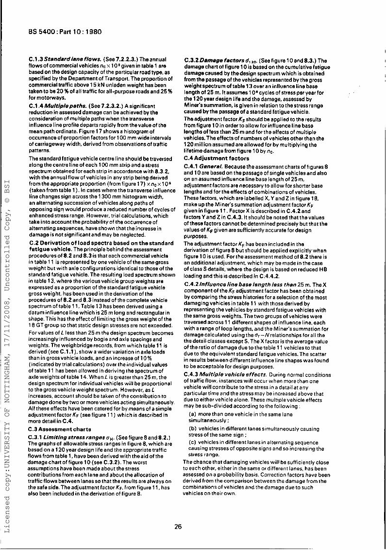
BS 5400 : Part 10 : 1980
C.1.3Stenderdlene flows. (See 7.2.2.3.) Theannual flows of commercial vehicles nc x 108 given in table 1 are based on the design capacity of the particular road type, as specified by the Department of Transport. The proportion of commercial traffic above 15 kN unladen weight has been taken to be 20 %of all traffic for all-purpose roads and 25 % for motorways. C.1.4 Multipleperhs. (See 7.2.3.2.) A significant reduction in assessed damage can be achieved by the consideration of multiple paths when the transverse influence line profile departs rapidly from thevalue of the mean path ordinate. Figure 17 shows a histogram of occurrence of proportion factors for 100 mm wide intervals of carriageway width, derived from observations of traftic patterns. The standard fatigue vehicle centre line should be traversed along the centre line of each 100 mm strip and a stress spectrum obtained for each strip in accordance with 8.3.2, with the annual flow of vehicles in any strip being derived from the appropriate proportion (from figure 17) xnc x 106 (taken from table 1 ). In cases where the transverse influence line changessign across the 1300 mm histogram width, an alternating succession of vehicles along paths of opposing sign would produce a reduced number of cycles of enhanced stress range. However, trial calculations, which take into account the probability of the occurrence of alternating sequences, have shown that the increase in damage is not significant and may be neglected. C.2 Derivat ion of load spectra based o n t h e standard fa t igue vehicle. The principle behind the assessment procedures of 8.2 and 8.3 is that each commercial vehicle in table 11 is represented by one vehicle of the same gross weight but with axle configurations identical to those of the standard fatigue vehicle. The resulting load spectrum shown in table 13, where the various vehicle group weights are expressed as a proportion of the standard fatigue vehicle gross weight, has been used in the derivation of the procedures of 8.2 and 8.3 instead of the complete vehicle spectrum of table 11. Table 13 has been derived using a datum influence line which is 25 m long and rectangular in shape. This has the effect of limiting the gross weight of the 18 GT group so that static design stresses are not exceeded. For values of L less than 25 m the design spectrum becomes increasingly influenced by bogie and axle spacings and weights. The weighbridge records, from which table 11 is derived (see C.1.1). show a wider variation in axle loads than in gross vehicle loads, and an increase of 10 % (indicated by trial calculations) over the individual values of table 11 has been allowed in deriving the spectrum of axle weights of table 14. When L is greater than 25 m, the design spectrum for individual vehicles will be proportional to the gross vehicle weight spectrum. However, as L increases, account should be taken of the contribution to damage done by two or more vehicles acting simultaneously. All these effects have been catered for by means of a simple adjustment factor KF (see figure 11 ) which is described in more detail in C.4. C.3 Assessment char ts C.3.1 Limiting stress ranges OH. (See figure 8 and 8.2.) The graphs of allowable stress ranges in figure 8, which are based on a 120 year design life and the appropriate traffic flowsfrom table 1, have been derived with theaid of the damage chart of figure 10 (see C.3.2). The worst assumptions have been made about the stress contributions from each lane and about the allocation of traffic flows between lanes so that the results are always on the safe side. The adjustment factor K F , from figure 11, has also been included in the derivation of figure 8.
C.3.2 Demege fectofs d , 20. (See figure 10 and 8.3.) The damage chart ot figure 10 is based on the cumulative fatigue damage caused by the design spectrum which is obtained from the passage of the vehicles represented by the gross weight spectrum of table 13 over an influence line base length of 25 m. It assumes 106 cycles of stress per year for the 120 year design life and the damage, assessed by Miner's summation, is given in relation to the stress range caused by the passage of a standard fatigue vehicle. The adjustment factor K F should be applied to the results from figure 10 in order to allow for influence line base lengths of less than 25 m and for the effects of multiple vehicles. The effects of numbers of vehicles other than the 120 million assumed are allowed for by multiplying the lifetime damage from figure 10 by nc. C.4 Adjus tment fac to rs C.4.1 Genere/. Because the assessment charts of figures 8 and 10 are based on the passage of single vehicles and also on an assumed influence line base length of 25 m, adjustment factors are necessary to allow for shorter base lengths and for the effects of combinations of vehicles. These factors, which are labelled X, Y and 2 in figure 18, make up the Miner's summation adjustment factor KF given in figure 1 1. Factor X is described in C.4.2 and factors Y and 2 in C.4.3. It should be noted that the values of these factors cannot be determined precisely but that the values of KF given are sufficiently accurate for design purposes. The adjustment factorKF has been included in the derivation of figure 8 but should be applied explicitly when figure 10 i s used. For the assessment method of 8.2 there is an additional adjustment, which may be made in the case of class S details, where the design is based on reduced H B loading and this is described in Ci4.4.2. C.4.2 Influence line bese length less then 25 m. The X component of the KF adjustment factor has been obtained by comparing the stress histories for a selection of the most damaging vehicles in table 11 with those derived by representing the vehicles by standard fatigue vehicles with the same gross weights. The two groups of vehicles were traversed across 11 different shapes of influence line, each with a range of loop lengths, and the Miner's summation for damage calculated using the Or -Nrelationships for al l the the detail classes except S. The X factor is the average value of theratio of damage due to the table 11 vehicles to that due to the equivalent standard fatigue vehicles. The scatter in results between different influence line shapes was found to be acceptable for design purposes. C.4.3 Multiple vehicle effects. During normal conditions of traff ic flow, instances will occur when more than one vehicle wil l contribute to the stress in a detail at any particular time and the stress may be increased above that due to either vehicle alone. These multiple vehicle effects may besub-divided according to the following :
(a) more than one vehicle in the same lane simultaneously ; (b) vehicles in different lanes simultaneously causing stress of the same sign ; (c) vehicles in different lanes in alternating sequence causing stresses of opposite signs and so increasing the stress range.
The chance that damaging vehicles will be sufficiently close to each other, either in the same or different lanes, has been assessed on a probability basis. Correction factors have been derived from the comparison between the damage from the combinations of vehicles and the damage due to such vehicles on their own.
26
Licensed copy:UNIVERSITY OF NOTTINGHAM, 17/11/2008, Uncontrolled Copy, © BSI
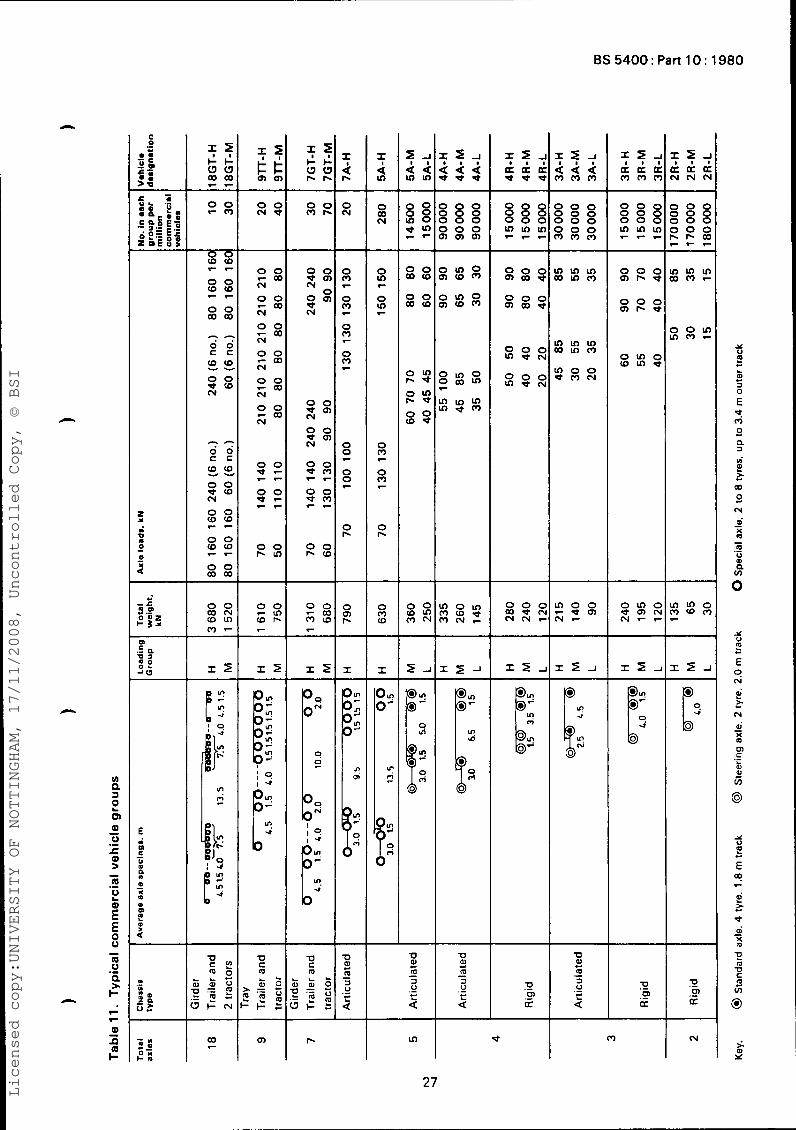
BS 5400 : Part 10 : 1980
5 % 5544
5% K K K m m m
? U m - 0 03 N
- 0 m
0 m
r
c
0 m
m
c
0 - 0 I-
- 0 co m
3 0 0 3 0 0 3 0 0 3 0 0 3 m m
0 0 0 0 0 0 0 0 0
3 0 0 3 0 0 3 0 0 ? X 8 r - l -
0 0 0 D O 0 0 0 0 3 0 0 m m m n m Q ) e r -
388 0 0 0
m m m - l - c
T 1-F
0 0 (Do
0 0 r c
m m
0 0
E 2
C I C
c c
0 0 bco N
h C
0 0
2 2 c c
0 0 dco N 0 0 z z 0 0 coo
0 0 C Q C O
F -
0 0 d Q ) N 0 oal
d N
0 0 d Q ) N 0 0 b Q ) N
0 0 e m r e
0 0 2:
0 0 (zco
0 m
m
m
m
c
0 e
0 l-
0 r
0 0
0 0
F
- 0 I-
- 0 Q) l-
c ) m m w m m 0 0 - 0 3 N 0 0 - 0 3 N 0 0 - 0 0 N
0 0 - 0 3 N 0 0 - 0 3 N 0 0 7 0 3 N
s z 2: - - 0 0
0 0 ( z m
n m m w m m
n o o b m ~
0 0 0 - d N
0 0 0 # d N
o m o c o m e
i m w 0 0
me4 c o r n - E L .-
m - c" i s n m o 3 w m r
n o o r e m N -
o m o b a r 4 N r l -
W .E n m o x z - I r z - l 1 I 1 1 1 1
rr! *
9 c (v
g,
- (P 0 P .- c"
A
P p m ID
0 a 0 .-
(v m d
27
Licensed copy:UNIVERSITY OF NOTTINGHAM, 17/11/2008, Uncontrolled Copy, © BSI
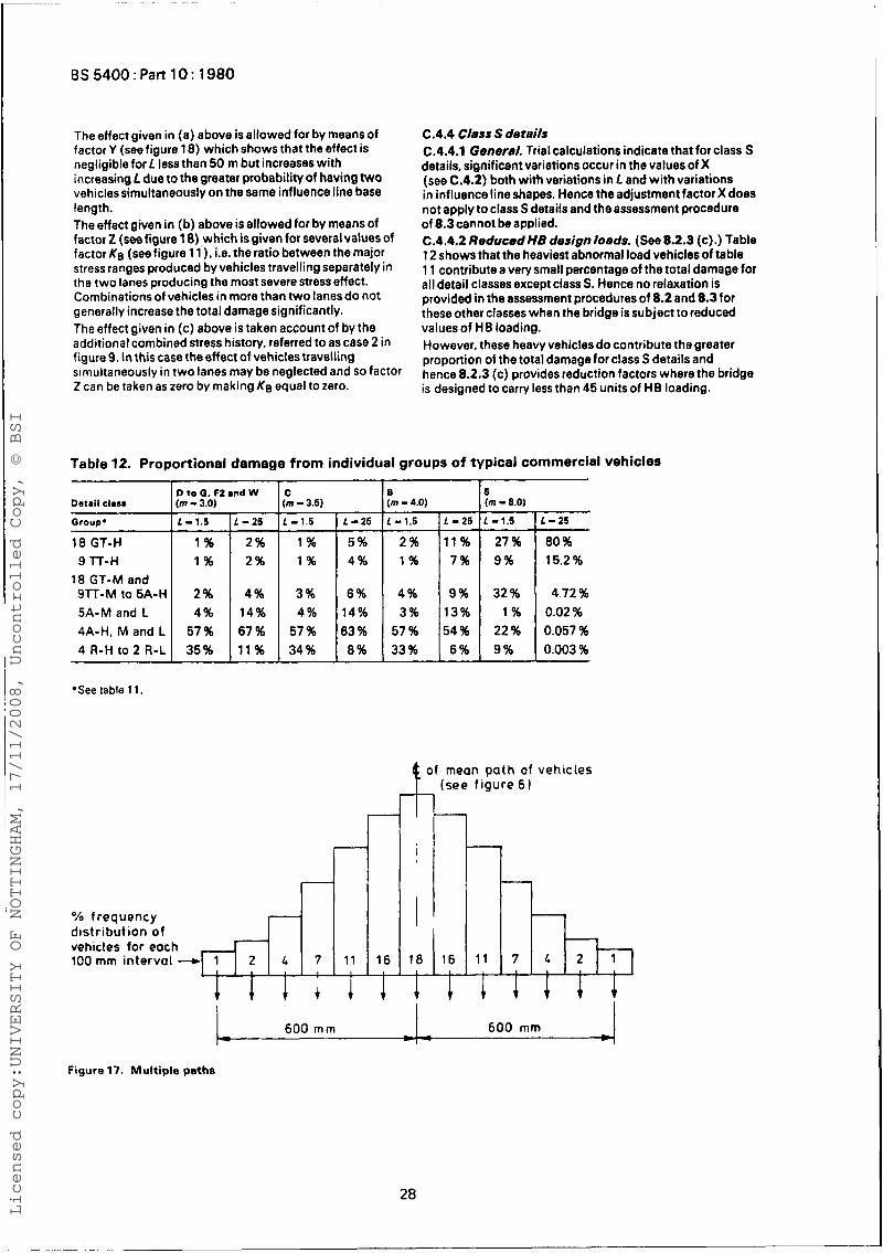
BS 5400 : Part 10 : 1980
The effect given in (a) above is allowed for by means of factor Y (see figure 18) which shows that the effect is negligible for L less than 50 m but increases with increasing L due to the greater probability of having two vehicles simultaneously on the same influence line base length. The effect given in (b) above is allowed for by means of factor 2 (see figure 18),which isgiven for severalvalues of factor Kg (see figure 11 ), i.e. the ratio between the major stress ranges produced by vehicles travelling separately in the two lanes producing the most severe stress effect. Combinations of vehicles in more than two lanesdo not generally increase the total damage significantly. The effect given in (c) above is taken account of by the additional combined stress history, referred to as case 2 in figure 9. In this case the effect of vehiclestravelling simultaneously in two lanes may be neglected and so factor Z can be taken as zero by making Ks equal to zero.
C.4.4 Class S details C.4.4.1 General. Trial calculations indicate that for class S details, significant variations occur in the values of X (see C.4.2) both with variations in L and with variations in influencelineshapes. Hence the adjustment factor X does not apply to class S details and the assessment procedure of 8.3 cannot be applied. C.4.4.2 ReducedHB designloeds. (See8.2.3 (c).) Table 12 shows that the heaviest abnormal load vehicles of table 1 1 contribute a very small percentage of the total damage for all detail classes except class S. Hence no relaxation is provided in the assessment procedures of 8.2 and 8.3for these other classes when the bridge is subject to reduced values of HB loading. However, these heavy vehicles do contribute the greater proportion of the total damage for class S details and hence 8.2.3 (c) provides reduction factors where the bridge is designed to carry less than 45 units of HB loading.
Table 12. Proportional damage from individual groups of typical commerclal vehicles
Dstril clrw
Group.
18 GT-H 9 lT -H
18 GT-M and
5A-M and L 4A-H, M and L
9lT- M to 5A- H
4 R - H to 2 R-L
D to a, Fisnd W 'm - 3.0)
14%
C m - 3.5)
! - 1.5
1% 1%
3% 4%
57 % 34 %
1 - 2 5 - 5% 4 %
6% 14% 63 % 8 %
% m - 4.0)
i - 1.5 L - 25 I' 13%
57% 54% 33% 6%
~~
i m - 8.0)
-1.5 I L - 2 5
0.057 % 0.003 %
'Seetablell.
of mean path of vehicles (see f igure 6 1
I I " I % frequency distribution of vehicles for each 100 mrn interval - 1
600 rnm 600 mm - ce c
Figure 17. Multiple paths
Licensed copy:UNIVERSITY OF NOTTINGHAM, 17/11/2008, Uncontrolled Copy, © BSI
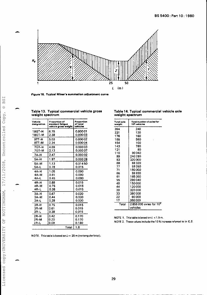
BS 5400 : Part 10 : 1980
18GT-M 9lT-H 9TT-M
c
2.38 0.000 03 5.03 0.000 02 2.34 0.000 04
c
7GT-M 7A-H 5A-H 5A-M
0
2.13 0.000 07 2.47 0.000 02 1.97 0.000 28 1.13 0.01 4 50
1
4R-H 4R-M 4R-L 3A-H 3A-M 3A-L
c
L
0.88 0.75 0.38 0.67 0.44 0.28
Figure 18. Typical Miner's summation adjustmont C U ~ V O
3R-H 0.75 3R-M 0.61
- Table 13. Typical commercial vehicle gross weight spectrum
0.01 5 0.01 5
Vehicle Proportion of Proportion of tote1 vehiclea
0.000 01
7GT-H 14.09 I 0.00003
0.01 5 0.090
4A- M 0.090 0.090 0.01 5 0.01 5 0.01 5 0.030 0.030 0.030
3R-L 10.38 I 0.015 2R-H 10.42 I 0.170 2R-M 0.20 0.1 70 2R-L 10.09 10.180
Table 14. Typical commercial vehicle axle weight spectrum
Total axle weight
264 231 176 165 154 143 121 110 99 93 88 77 71 66 61 55 49 44 39 33 22 17
Total
Totalnumber of exlerfor 106 vohicloa
240 120 160 560 100 780 80
90 040 240 280 320 000 59 320 59 350
1 80 000 59 930
1 65 000 290 040 1 50 000 1 20 000 320 000 380 000 60 000
360 000 2 856 000 axles for 10' vehicles
NOTE 1. This table is based on L < 1.5 m. NOTE 2. Thesevaluesinclude the 10 %increase referred to in C.2.
Total I 1.0
NOTE. This table is based on L = 25 m (rectangular loop).
29
Licensed copy:UNIVERSITY OF NOTTINGHAM, 17/11/2008, Uncontrolled Copy, © BSI
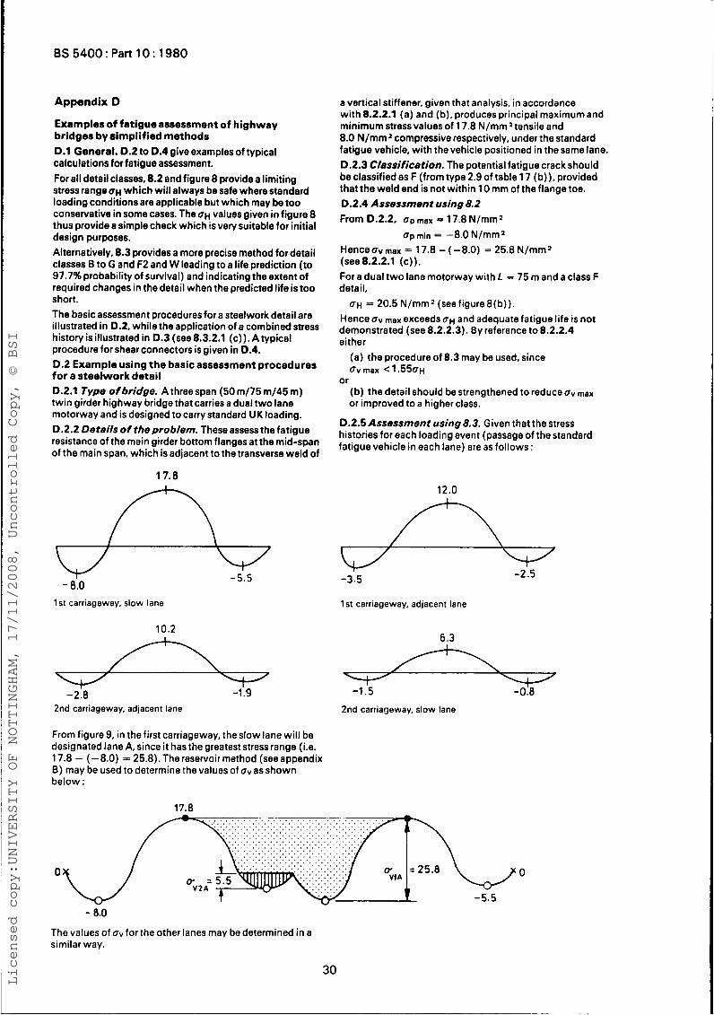
~
Appendix D
Examples of fatigue assessment o f highway bridges by simplif ied methods D.l General. D.2 to D.4 give examples of typical calculations for fatigue assessment. For all detail classes, 8.2 and figure 8 providea limiting stress range QH which will always be safe where standard loading conditions are applicable but which may be too conservative in some cases. The UH values given in figure 8 thus provide a simple check which is very suitable for initial design purposes. Alternatively, 8.3 provides a more precise method for detail classes B to G and F2 and W leading to a life prediction (to 97.7% probability of survival) and indicating the extent of required changes in thedetail when the predicted life is too short. The basic assessment procedures for a steelwork detail are illustrated in 0.2, while the application of a combined stress history is illustrated in D.3 (see8.3.2.1 (c)). Atypical procedure for shear connectors is given in D.4. D.2 Example using the basic assessment procedures f o r a steelwork detail 0.2.1 Type of bridge. A three span (50 m/75 m/45 m) twin girder highway bridge that carries a dual two lane motorway and is designed to carry standard UK loading. D.2.2 Details of theproblem. These assess the fatigue resistance of the main girder bottom flanges at the mid-span of the main span, which is adjacent to the transverse weld of
17.8
a vertical stiffener, given that analysis, in accordance with 8.2.2.1 (a) and (b), produces principal maximumand minimum stressvalues of 17.8 Nlrnmz tensile and 8.0 N/mm compressive respectively, under the standard fatigue vehicle, with the vehicle positioned in thesame lane. D.2.3 Classification. The potential fatigue crack should be classified as F (from type 2.9 of table 17 (b)), provided that the weld end is not within 10 mm of the flange toe. 0.2.4 Assessment using 8.2 From D.2.2, op may = 17.8 N/mm2
UP min = -8.0 N/mm2 Henceuv max = 17.8 - ( -8.0) = 25.8 N/mm2 (see8.2.2.1 (c)). Fora dual two lane motorway with L = 75 m and a class F detail,
Hence UV max exceeds OH and adequate fatigue life is not demonstrated (see 8.2.2.3). By reference to 8.2.2.4 either
U H = 20.5 N/mm’(seefigure8(b)).
(a) the procedure of 8.3 may be used, since uv max < 1 .55~H
(b) the detail should be strengthened to reduce UV max or improved to a higher class.
or
D.2.5Assessment using8.3. Given thatthe stress histories for each loading event (passage of the standard fatigue vehicle in each lane) are as follows:
- 8.0 1 st carriageway, slow lane 1 st carriageway, adjacent lane
d -2.8 -1.9 7 -1.5 -0.8
2nd carriageway, adjacent lane 2nd carriageway, slow lane
From figure 9, in the first carriageway, the slow lane will be designated lane A, since it has the greateststress range (i.e. 17.8 - (-8.0) = 25.8).The reservoir method (seeappendix 6) may be used to determine the values of oV as shown below :
17.8
0 0
- 8.0
The values of uv for the other lanes may be determined in a similar way.
30
Licensed copy:UNIVERSITY OF NOTTINGHAM, 17/11/2008, Uncontrolled Copy, © BSI
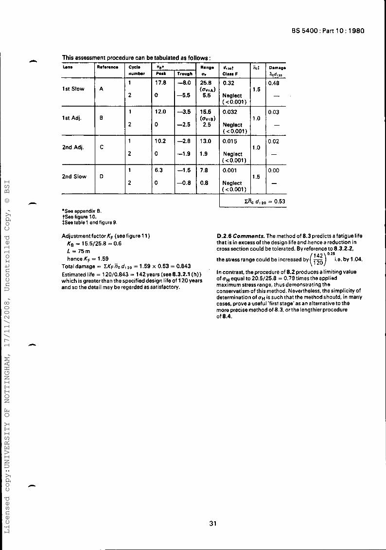
BS 5400: Part 10: 1980
This assessment procedure can be tabulated as follows : &:
1.5
1 .o
1 .o
t
numkr
1st Slow
Domigo
0.48 &d,m
- 0.03
-
0.02
-
1 l 2
2nd Adj.
I I I
1
2 C
2nd Slow
*D.
P u k
17.8
0
12.0
0
10.2
0 ,=:
4 10 t C l i u F
0.32
Neglect ( < 0.001 )
0.032
Neglect ( c 0.001 )
0.01 5
Neglect ( < 0.001 ) ,"'" 1-1.5 I 7.8 1 0.001 IlS5 10:
-0.8 0.8 Neglect ( < 0.001 )
*See appendix B. tSee figure 10. #See table 1 and figure 9.
Adjustment factor K, (see figure 11) KB = 15.5/25.8 = 0.6 1 = 7 5 m hence KF = 1.59
D.2.6 Comments. The method of 8.3 predicts a fatigue life that is in excess of the design life and hence a reduction in cross section could be tolerated. By reference to 8.3.2.2,
the stress range could be increased by (142 \ o'2si.e. by 1.04. - . \ ILV/ Total damage = ZKF EC d , 2o = 1.59 x 0.53 = 0.843 Estimated life = 2010.843 =i 4zyears (see 8.3.2.1 (h)) which is greater than the specified design life of 120years and so the detail may be regarded as satisfactory.
In contrast, the procedure of 8.2 produces a limiting value Of uH equal to 20*5/25.8 = 0.79 times the applied maximum stress range, thus demonstrating the conservatism of this method. Nevertheless, the simplicity of determination of OH is such that the method should, in many cases, prove a useful 'first stage'as an alternative to the more precise method of 8.3, or the lengthier procedure of 8.4.
31
Licensed copy:UNIVERSITY OF NOTTINGHAM, 17/11/2008, Uncontrolled Copy, © BSI
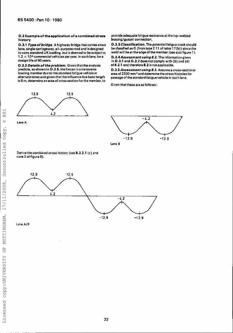
12.9 12.9
0.3 Example of the application of a combined stress history D.3.1 Typeofbridge. A highway bridge that carriesa two lane, single carriageway, all-purpose road and is designed to carry standard UK loading, but is deemed to be subject to 1.2 x 10⁶ commercial vehicles per year, in each lane, for a design life of 60 years. 0.3.2 Details of theproblem. Given that the analysis predicts, as shown in D.3.5, the forces in a transverse bracing member due to the standard fatigue vehicle in alternate lanes and given that the influence line base length is 8 m, determine an area of cross section for the member, to
provide adequate fatigue resistance at the lap-welded bracinglgusset connection. D.3.3 Cl8ssification. The potential fatigue crack should beclassfiedasG (fromtype2.11 oftable17(b)) sincethe
,weld will beattheedgeofthemember (seealsofigurel). D.3.4Asssssm8nt using8.2. The information given in D.3.1 and D.3.2 does not comply with (b) and (d) of 8.2.1 and therefore 8.2 is not applicable. D.3.5 Assessment using8.3. Assume a cross-sectional area of 2200 mmz and determine the stress histories for passage of the standard fatigue vehicle in each lane.
Given that these are as follows :
Lane A
- 12.9 -12.9 Lane B
Derive the combined stress history (see 8.3.2.1 (c) and case 2 of figure 9).
12.9 12.9
- 12.9 -1 2.9
Lane A/B
32 Licensed copy:UNIVERSITY OF NOTTINGHAM, 17/11/2008, Uncontrolled Copy, © BSI
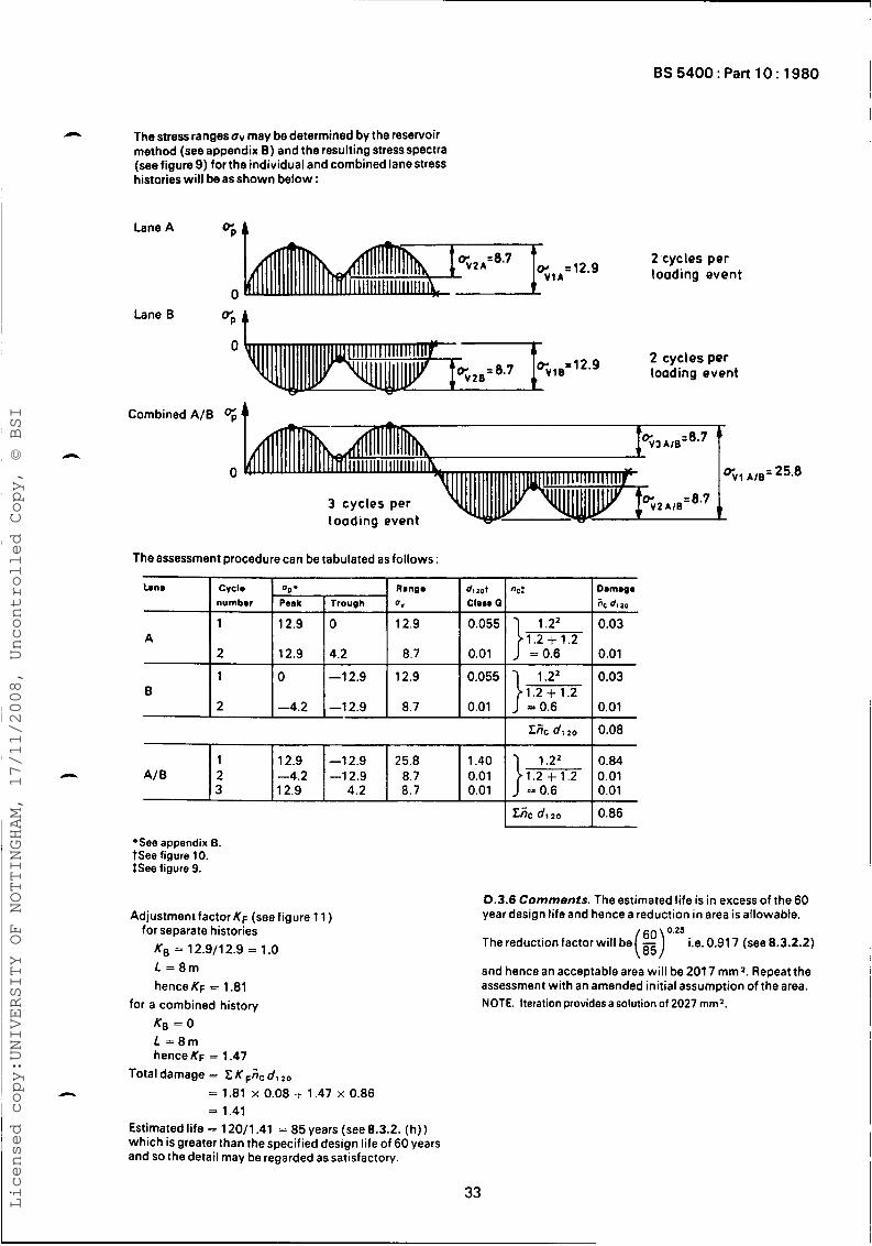
0
-4.2
-1 2.9
-12.9
n The stress ranges uv may be determined by the reservoir method (see appendix B) and the resulting stress spectra (see figure 9) for the individual and combined lane stress histories wil l be as shown below :
54 Lane A
Z'cycles per loading event
0
"Pt Lane B
0 2 cycles per loading event
Combined A/B 4 A ,, A,B= 25.8
The assessment procedure can be tabulated as follows
"C! Lene
A
CVCI. number
1
2
Range
OV
12.9
8.7
Damaga
fie d i z o
0.03
0.01
dttot Claaa 0
0.055
0.01 }I.;.:.,, = 0.6
12.9 14.2
1
2
12.9
8.7
0.055
0.01
0.03
0.01 } 1 .; :21 .2
= 0.6 B
0.08 I I
0.84 0.01 0.01
1 .; :zl .2 = 0.6
Z& dc ao 0.86
*See appendix E. tSee figure 10. $See figure 9.
0.3.6 Comments. The estimated life is in excess of the 60 year design life and hence a reduction in area i s allowable.
The reduction factor will be( g) 0.21
i.e. 0.91 7 (see 8.3.2.2)
Adjustment factor K F (see figure 11) for separate histories
KO = 12.911 2.9 = 1 .O . . L = 8 m henceKF = 1.81
and hence an acceptable area will be 201 7 mm2. Repeat the assessment with an amended initial assumption of the area. NOTE. Iteration provides a solution of 2027 mm2. for a combined history
KB = 0 L = 8 m hence KF = 1.47
Total damage = Z K d , 2o
LI = 1.81 x 0.08 -7 1.47 x 0.86 = 1.41
Estimated life = 12011.41 = 85 years (see 8.3.2. (h)) which is greater than the specified design life of 60 years and so the detail may be regarded as satisfactory.
33
Licensed copy:UNIVERSITY OF NOTTINGHAM, 17/11/2008, Uncontrolled Copy, © BSI
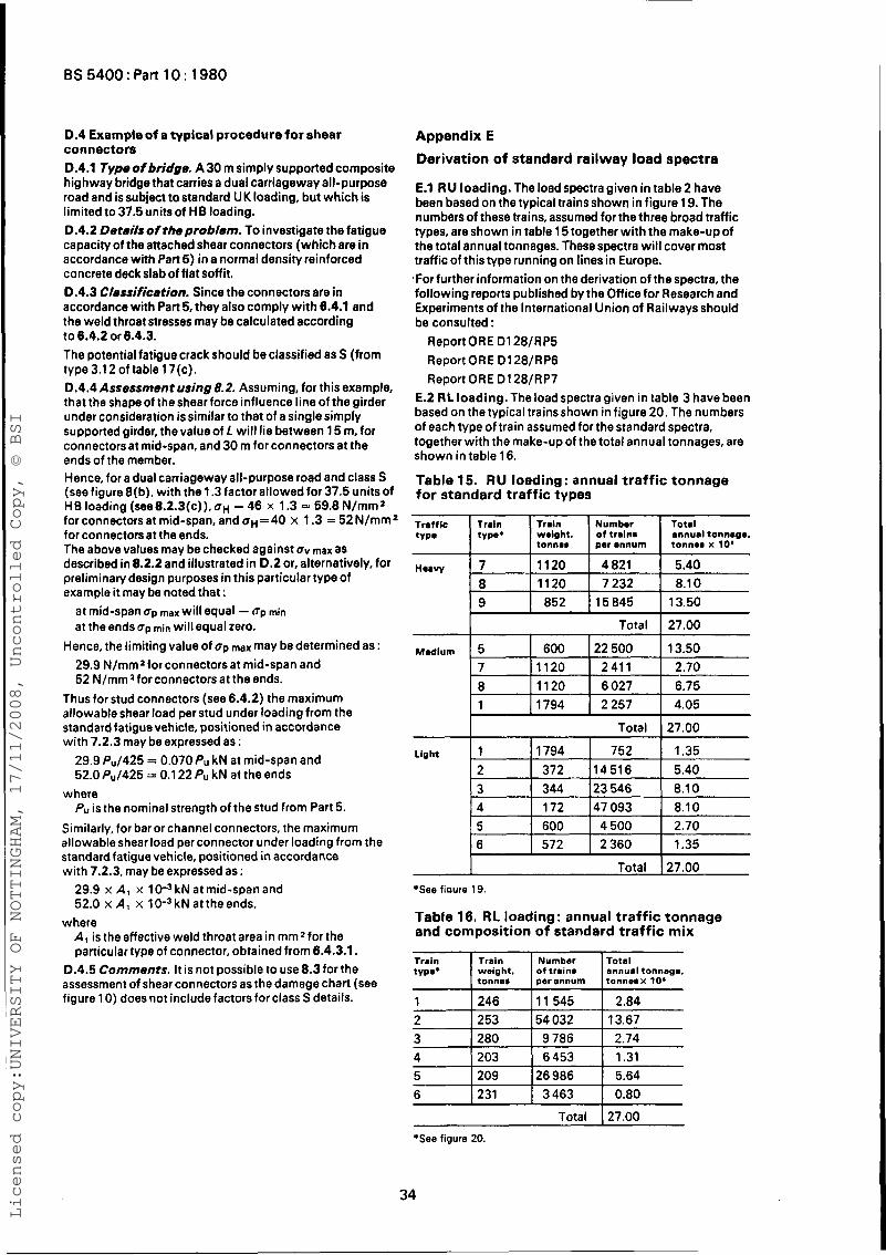
0.4 Exampleof a typical procedure for shear connectors D.4.1 Type of bridge. A 30 m simply supported composite highway bridge that carries a dual carriageway all-purpose road and is subject to standard U K loading, but which is limited to 37.5 units of HB loading. D.4.2 Detailsof theproblem. To investigate the fatigue capacity of the attached shear connectors (which are in accordance with Part 5) in a normal density reinforced concrete deck slab of flat soff it. D.4.3 Clessification. Since the connectors are in accordance with Part 5, they also comply with 6.4.1 and the weld throat stresses may be calculated according to 6.4.2 or 6.4.3. The potential fatigue crack should be classified as S (from type3.12oftable17(c). D.4.4 Assessment using 8.2. Assuming, for this example, that the shapeof the shear force influence line of the girder under consideration is similar to that of a single simply supported girder, the value of L will lie between 15 m, for connectors at mid-span, and 30 m for connectors at the ends of the member. Hence, for a dual carriageway all-purpose road and class S (seefigureB(b). withthe 1.3factorallowedfor37.5unitsof HB loading (see8.2.3(c)), OH - 46 x 1.3 = 59.8 N/mm2 for connectors at mid-span, and u ~ = 4 0 x 1.3 = 52N/mmZ for connectors at the ends. The above values may be checked against uv max as described in 8.2.2 and illustrated in D.2 or, alternatively, for preliminary design purposes in this particular type of example it may be noted that:
at mid-span up max will equal - OP min at the ends bp min will equal zero.
29.9 N/mm'for connectors at mid-span and 52 N/mmZforconnectorsat theends.
Thus for stud connectors (see 6.4.2) the maximum allowable shear load per stud under loading from the standard fatigue vehicle, positioned in accordance with 7.2.3 may be expressed as :
29.9 Pu/425 = 0.070 PU kN at mid-span and 52.0 Pu/425 = 0.1 22 Pu kN at the ends
where Puis the nominal strength of the stud from Part 5.
Similarly, for bar or channel connectors, the maximum allowable shear load per connector under loading from the standard fatigue vehicle, positioned in accordance with 7.2.3, may be expressed as:
Hence, the limiting value of b p max may be determined as :
29.9 x A, x lC3 kN at mid-span and 52.0 x A, x lC3 kN attheends.
A, is the effective weld throat area in mm2for the particular type of connector, obtained from 6.4.3.1.
D.4.5 Comments. It is not possible to use 8.3 for the assessment of shear connectors as the damage chart (see figure 10) does not include factors for class S details.
where
8 1
Appendix E
Der ivat ion of standard railway load spectra
E.l RU loading. The load spectra given in table 2 have been based on the typical trains shown in figure 19. The numbers of these trains, assumed for the three broad traffic types, are shown in table 15 together with the make-up of the total annual tonnages. These spectra will cover most traffic of this type running on lines in Europe. 'For further information on the derivation of the spectra, the following reports published by the Office for Research and Experiments of the International Union of Railways should be consulted :
Report ORE D128/RP5 Report ORE D128/RP6 Report ORE D128/RP7
E.2 RL loading. The load spectra given in table 3 have been based on the typical trains shown in figure 20. The numbers of each type of train assumed for the standard spectra, together with the make-up of the total annual tonnages, are shown in table 16.
Table 15. RU loading: annual t r a f f i c t onnage for standard traffic types
1120 6027 6.75 1794 2 257 4.05
Traffic 1 Train 1 Trrln 1 Numbor 1 Total WP. typo. wolght, of trains annual tonnage,
tonnrs par annum tonnes x 10'
Horvy
Medium 5 I 600 122500 I 13.50 7 11120 I 2411 I 2.70
l ight
14516 5.40 8.1 0
4 I 172 (47093 I 8.10 5 I 600 I 4 500 I 2.70
I 572 I 2360 I 1.35 I 6
1 Total 127.00 *See fiaure 19.
Table 16. RL loading: annual t r a f f i c t onnage a n d composition of standard t r a f f i c m i x
Train type. 1 i!:;, 1 FcK I tonnage,
perannum tonneax 10'
1 I246 111 545 I 2.84 2 I253 I54 032 I 13.67 3 I280 I 9786 I 2.74 4 I203 I 6453 I 1.31
26 986
+See figure 20.
34
Licensed copy:UNIVERSITY OF NOTTINGHAM, 17/11/2008, Uncontrolled Copy, © BSI
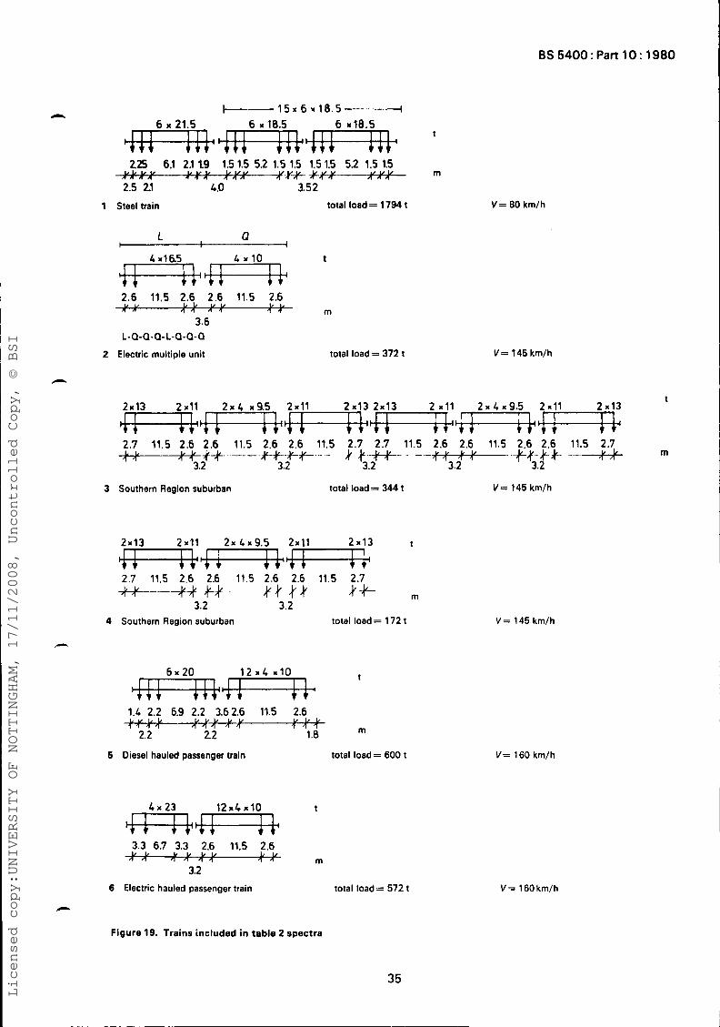
BS 5400: Part 10: 1980
225 6.1 21 1.9 1.5 1.5 5.2 1.5 1.5 1.5 1.5 5.2 1.5 1.5 l#u b U b l0vv n * 4 1 - 4 1 . 4 Y#**H---+++-
2.5 21 L .O 3.52 1 Steel train total load = 1794 t V = 80 km/h
L Q r I
t
e F + + F = % 2.6 11.5 2.6 2.6 11.5 2.6
3.6 i m
L-a-a-a-L-a-a-a 2 Electric multiple unit total load = 372 t V = 145 km/h
2.7 11.5 2.6 2.6 11.5 2.6 2.6 11.5 2.7 2.7 11.5 2.6 2.6 11.5 2.6 2.6 11.5 2.7
3.2 3.2 3.2 3.2 3.2 .++-#+ ---$-$-+.$- - k +-3c7(L- --$+++--. -;1Ly-+$- --IoL m
3 Southern Region suburban total load = 344 t V = 145 km/h
2.7 11.5 2.6 2.6 11.5 2.6 2.6 11.5 2.7 +t----H 3L# - $ 4 t t k+ m
3.2 3.2 4 Southern Region suburban total load = 172 t
1 1 , t 12 x L n10
e , i 1 + + 1.1 2.2 6.9 2.2 3.62.6 11.5 2.6
++++++- 1.0 m 2.2 22
5 Diesel hauled passenger train total load = 600 t
3.3 6.7 3.3 2.6 11.5 2.6 p m
3.2 6 Electric hauled passenger train total load = 572 t
Figure 19. Trains included in table 2 spectra
35
V = 145 km/h
V = 160 km/h
V = 160 km/h
Licensed copy:UNIVERSITY OF NOTTINGHAM, 17/11/2008, Uncontrolled Copy, © BSI
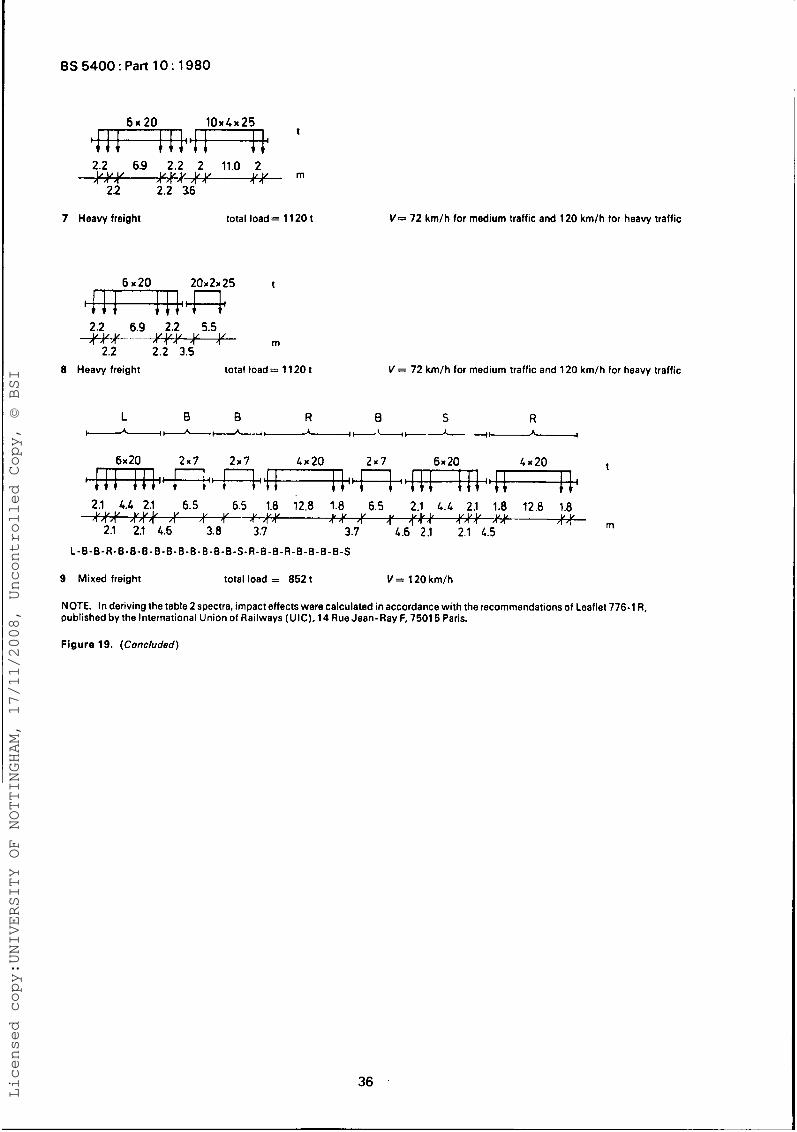
I BS 5400: Part 10: 1980
9. 6.9 2.2 2 11.0 2 m
2 2 2.2 36
7 Heavy freight total load = 1 120 t V = 72 km/h for medium traffic and 120 km/h tor heavy traffic
2.2 6.9 2.2 5.5 +++-.--- m 2.2 2.2 3.5
8 Heavy freight total load = 11 20 t V = 72 km/h for medium traffic and 120 km/h for heavy traffic
Lx20 6x20 6x20 t 6x20
~~
1:: +%+!: !2n7:::; I 1:: +&+ : : ~ , ,11 1. t( 2.1 4.L 2.1 6.5 1.8 12.8 1.8 6.5 2.1 L.L 26 1.8 12.8 1.8
* v v ” L I b b V L I / Y L , U P 1 1 ‘I 1 11-7 4 4 1 6 4 1 q m
2.1 2.1 4.6 3.8 3.7 3.7 4.6 21 2.1 4.5 L - B - B - R - B - B - B - B - ~ ~ B - B - B - B - B - S - R ~ B - B - R ~ B - 0 - B - B - S
9 Mixed freight total load = 852 t V = 120km/h
NOTE. In deriving the table 2 spectra, impact effects were calculated in accordance with the recommendations of Leaflet 776-1 R, published by the International Union of Railways (UIC), 14 Rue Jean-Ray F, 7501 5 Paris.
Figure 19. (Concluded)
36
Licensed copy:UNIVERSITY OF NOTTINGHAM, 17/11/2008, Uncontrolled Copy, © BSI
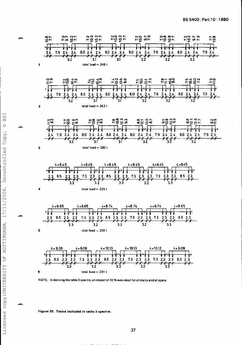
2.4 7.9 2.4 2.4 8.0 2.4 2.4 8.0 2.1 2.4 8.0 2.4 2.4 7.9 2.4 2.4 8.0 2.4 2.L 7.9 2.L
3.2 3.1 3.1 3.2 3.2 3.2 v v v V V V
A I 4 4 4 4 A A 4 4 4 4 A 4 4 4 A A 4 A A 4 1/1 4 4 A
1 total load = 246 t
NO *rn rn- 90 In- O N 9?
%.L 7.9 2.4 2.L 8.0 2.4, 2.L 8.0 2.L z . 4 8.0 2.4 2.4 7.9 2 . t b4 8.0 2.t 2.4 7.9 $4 4 4 4 4 4 4 4 4 4 4 4 4 4 4 4 4 1 1 / I n
3.21 3.2 3.7 ’ I 3 1 3.2 3.2 2 total load = 253 t
Lx8.65 Lx8.74 L x8.7L Lx8.74 Lx8.65
2.3 8.5 2.3 2.3 7.3 2.3 2.3 8.5 2 3 , 2.3 7.3 2.3 2.3 7.3 2.3 2.3 8.5 2.3
3.3 3.2 3.3 3 2 3.3 U
A 4 4 1 A 4 4 4 A A / r 4 A A A A 1 4 4 4 f l f l 4 4
5 total load = 209 t
L x 9.08 L 9.08 Lx 10.13 L x 10.13 LxlO.13 L x 9.08
2.3 8.5 2.3 2.3 7.3 2.3 2.3 8.5 2.3 2.3 7.3 2.3 2.3 7.3 2.3 2.3 8.5 2.3 w v U v u U
4 4 4 4 4 4 A A A A 4 4 n 4 A 4 3.3 3.2 3.3 3.2 /I 3 . 3
1 4
6 total load = 231 t
NOTE. In deriving the table 3 spectra, an impact of 3 0 %was taken for all trains and all spans
Figure 20. Trains included in table 3 spectra.
37
Licensed copy:UNIVERSITY OF NOTTINGHAM, 17/11/2008, Uncontrolled Copy, © BSI
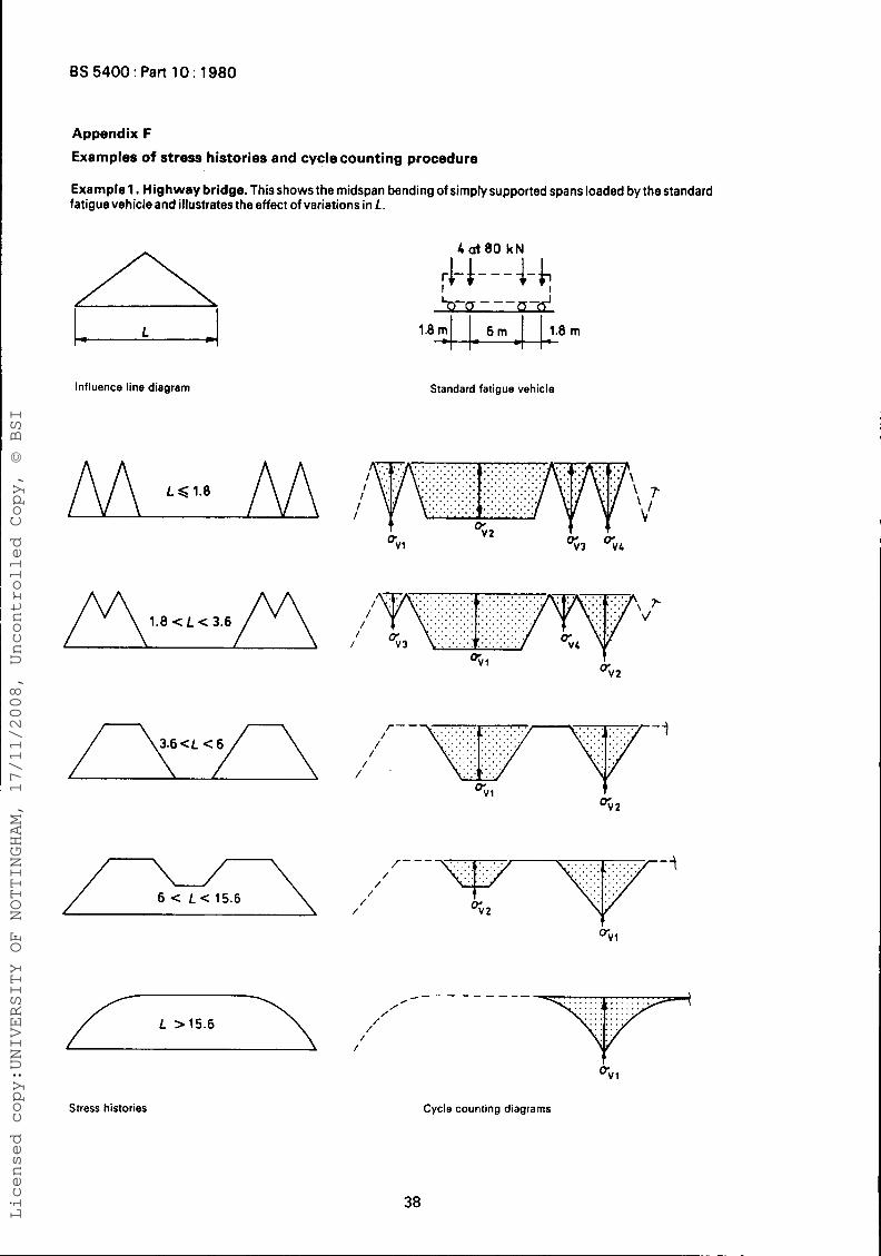
Appendix F
Examples of stress histories and cycle counting procedure
Example 1. Highway bridge. This shows the midspan bending of simply supported spans loaded by the standard fatigue vehicle and illustrates the effect of variations in L.
Influence line diagram
L < 1.8
1.8 < L < 3.6
4 a t 8 0 k N
4- I i- - - - 4- 1 . 8 4 6 m I J.8 m
Standard fatigue vehicle
I
/-\<'<n ,,/,I, r - - -w--y--j t.,.,.,'.'.' ..'.'.'...'. . . . . . . . . . . . . . . . . . . . . . . . . . . . . . . . . . . . . . . , . . . . . . . . .
. . . . . . . . . e", ..
Qv2
6 < L < 15.6 / 5 2
otl
ot 1
Stress histories Cycle counting diagrams
38
Licensed copy:UNIVERSITY OF NOTTINGHAM, 17/11/2008, Uncontrolled Copy, © BSI
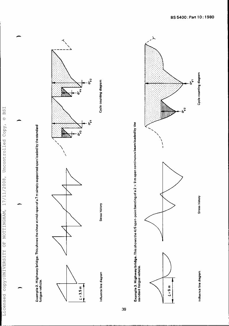
E m U C m U) Q
> U Q U m 0 C m
U 0)
c
5 n
- :: z n n
CI
3 U)
z - .- e U)
E r- m 0 C m
r
n ? x E c
L m m Q c U)
Q 5 : c U) U)
c + 0
.-
ai ‘0 n L
\ .(
\
\ \
‘\ \ \
N
-b’
- b’
E e m CO U m c C
0 0 Q
U
.-
.- c a
- Y
0)
>. U al
5 n
B - 5 Q
U) 3 0 3 C
C
n
.- c 8 e C m
E Q)
X FI m 0 WJ C U C 9)
u-
.-
n
x 0
/
c
23’
\ I
c $ U)
E
39
Licensed copy:UNIVERSITY OF NOTTINGHAM, 17/11/2008, Uncontrolled Copy, © BSI
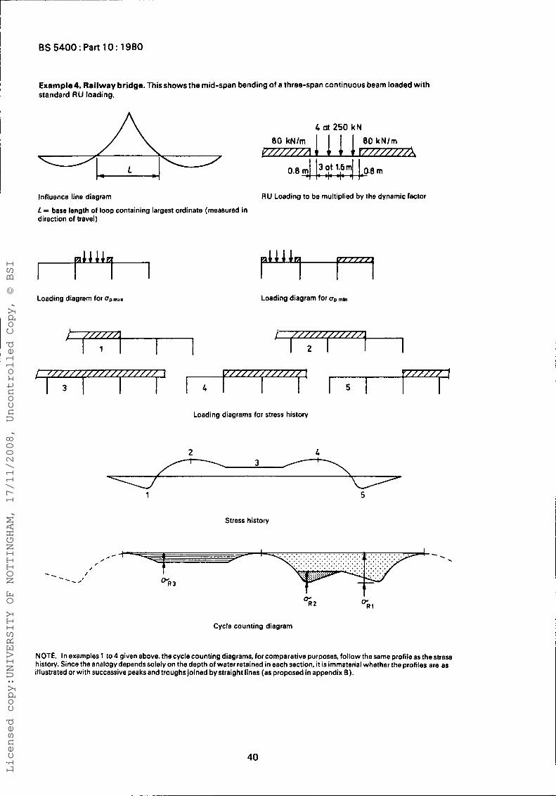
BS 5400: Part 10: 1980
Exemple4. Railway bridge. This shows the mid-span bending of a three-span continuous beam loaded with standard RU loading.
Influence line diagram
L = base length of loop containing largest ordinate (measured in direction of travel)
Loading diagram for uDml,.
4 at 250 kN 80 kNlm 80 k N l m
RU Loading to be multiplied by the dynamic factor
Loading diagram for up min
Loading diagrams for stress history
2 3
1
Stress history
, - - / t
. . r , - /
/
pR 3 . -.
Cycle counting diagram
40
NOTE. In examples 1 to 4 given above, the cycle counting diagrams, for comparative purposes, follow the same profile as the stress history. Since the analogy dependssolely on the depth of water retained in each section, it is immaterial whether the profiles are as illustrated or with successive peaks and troughs joined by straight lines (as proposed in appendix 6 ) .
Licensed copy:UNIVERSITY OF NOTTINGHAM, 17/11/2008, Uncontrolled Copy, © BSI
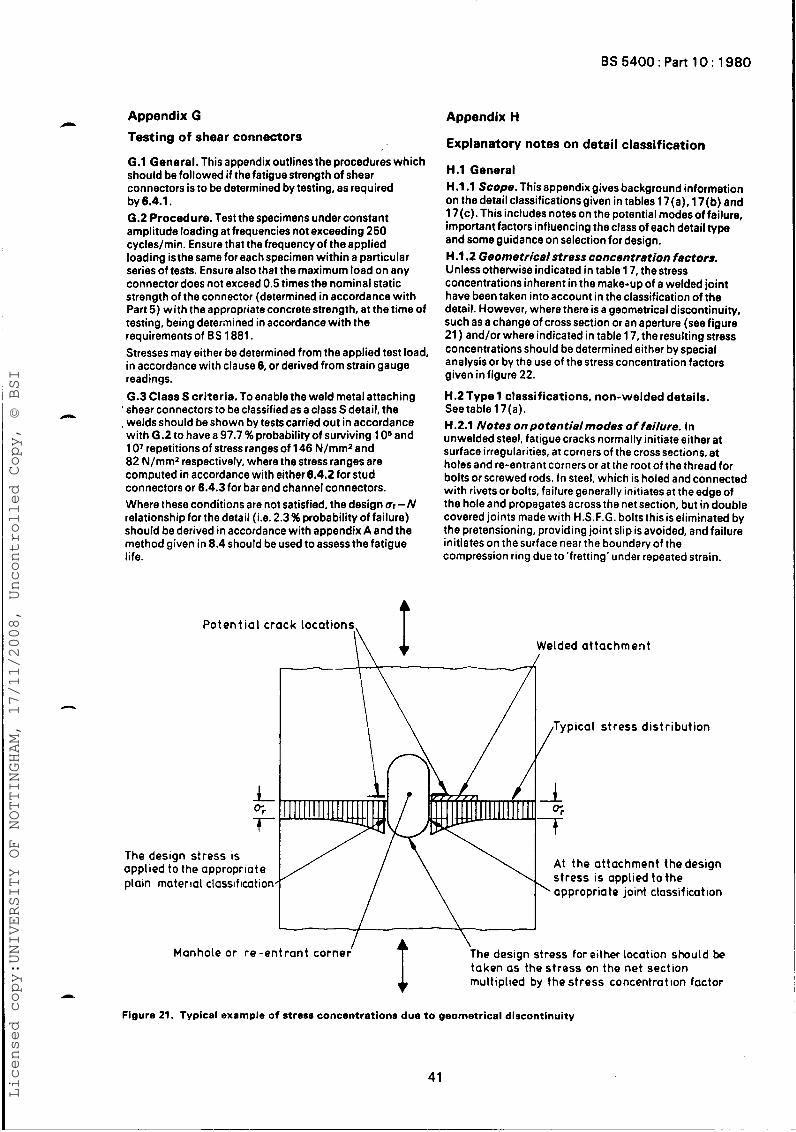
Appendix G Testing of shear connectors
- G.l General. This appendix outlines the procedures which should be followed i f the fatigue strength of shear connectors is to be determined by testing, as required by 6.4.1. 6.2 Procedure. Test the specimens under constant amplitude loading at frequencies not exceeding 250 cycles/min. Ensure that the frequency of the applied loading isthe same for each specimen within a particular series of tests. Ensure also that the maximum load on any connector does not exceed 0.5 times the nominal static strength of the connector (determined in accordance with Part 5) with the appropriate concrete strength, at the time of testing, being determined in accordance with the requirements of BS 1881. Stresses may either be determined from the applied test load, in accordance with clause 6, or derived from strain gauge readings. 6.3 Class S criteria. To enable the weld metal attaching
’ shear connectors to be classified as a class S detail, the , welds should be shown by tests carried out in accordance withG.2to havea97.7%probabilityofsurviving 106and 107 repetitions of stress ranges of 146 Nlrnm’ and 82 N/mm2 respectively, where the stress ranges are computed in accordance with either 6.4.2 for stud connectors or 6.4.3for bar and channel connectors. Where these conditions are not satisfied, the design a,-N relationship for the detail (i.e. 2.3 % probability of failure) should be derived in accordance with appendix A and the method given in 8.4 should be used to assess the fatigue life.
-
A
Appendix H
Explanatory notes on detail classification
H.l General H.l.l Scope. This appendix gives background information on thedetail classificationsgiven in tables 17(a), 17(b) and 17(c). This includes notes on the potential modes of failure, important factors influencing the class of each detail type and some guidance on selection for design. H .1.2 Geometricalstress concentration factors. Unlessotherwise indicated in table 17, thestress concentrations inherent in the make-up of a welded joint have been taken into account in the classification of the detail. However, where there is a geometrical discontinuity, such as a change of crosssection or an aperture (see figure 21 ) and/or where indicated in table 17, the resulting stress concentrations should be determined either by special analysis or by the use of the stress concentration factors given in figure 22.
H.2 Type 1 classifications, non-welded details. See table 1 7 (a). H.2.1 Notes onpotentialmodes of failure. In unwelded steel, fatigue cracks normally initiate either at surface irregularities, at corners of the cross sections, at holes and re-entrant corners or at the root of the thread for bolts or screwed rods. In steel, which is holed and connected with rivets or bolts, failure generally initiates at the edgeof the hole and propagates across the net section, but in double covered joints made with H.S.F.G. bolts this is eliminated by the pretensioning, providing joint slip is avoided, and failure initiates on the surface near the boundary of the compression ring due to ‘fretting’ under repeated strain.
Potent ia l crack locations nl Welded attachment /
ypical stress distribution
The design stress is applied to the appropriate plain material classification
At the attachment thedesign stress is applied to the appropriate joint classification
The design stress for either location should be taken as the stress on the net section multiplied by the stress concentration factor I /
Manhole or re-ent rant corner
Figure 21. Typical example of stress concentrations due to geometrical discontinuity
41
Licensed copy:UNIVERSITY OF NOTTINGHAM, 17/11/2008, Uncontrolled Copy, © BSI
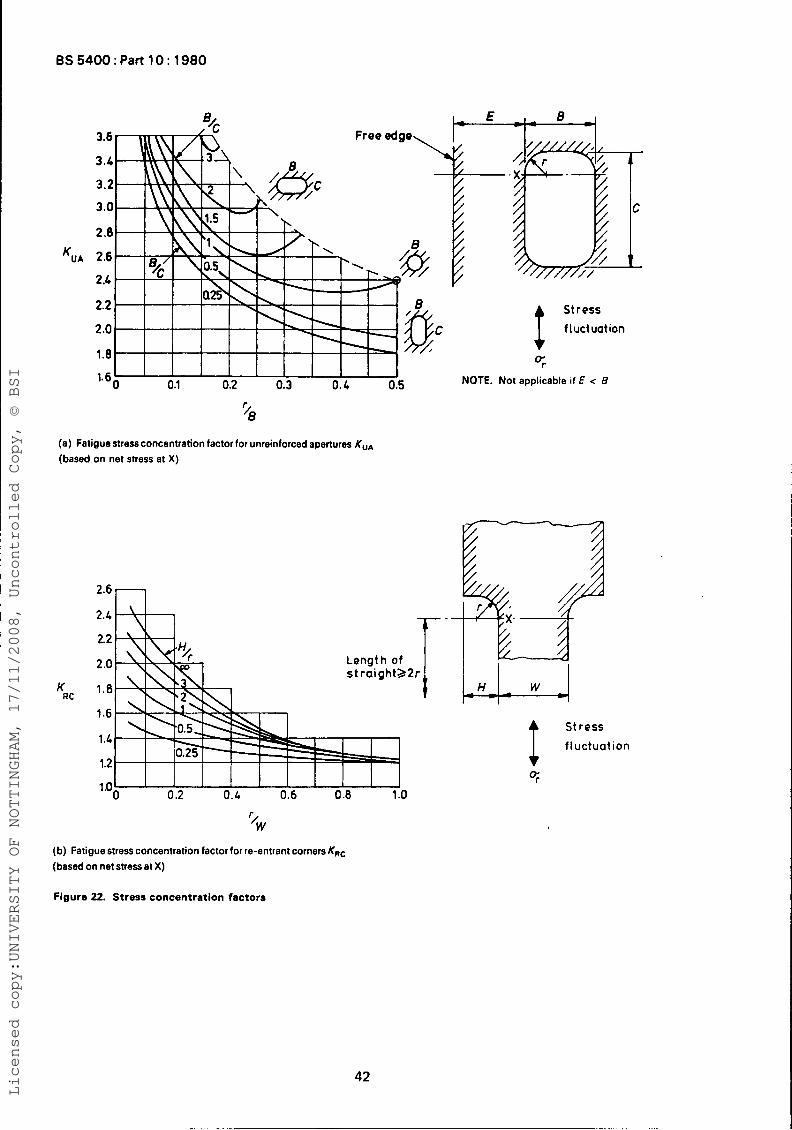
BS 5400: Part 10: 1980
(a) Fatigue stress concentration factor for unreinforced apertures KUA (based on net stress at X)
K RC
%v (b) Fatigue stress concentration factor for re-entrant corners KRc (based on net stress at X)
Length of st raight22r
H W
Stress fluctuation
0;
Figure 22. Stress concentration factors
42
Licensed copy:UNIVERSITY OF NOTTINGHAM, 17/11/2008, Uncontrolled Copy, © BSI
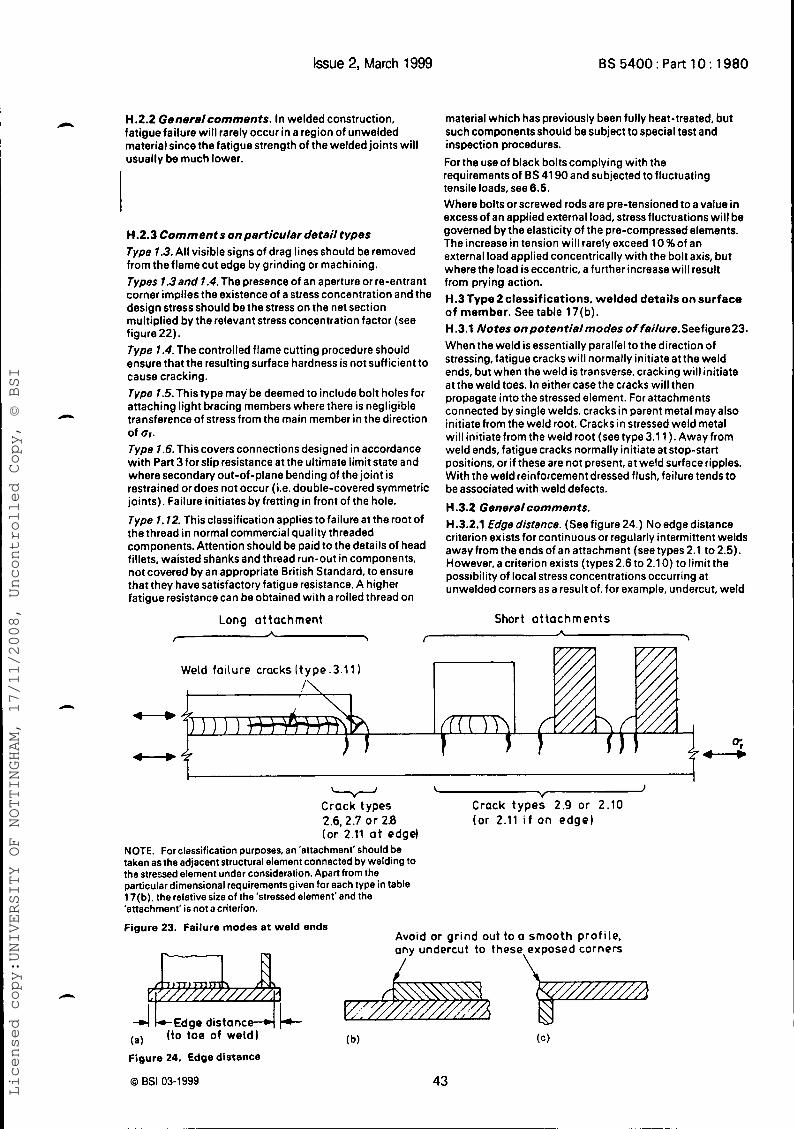
Issue 2, March 1999 BS 5400: Part 10: 1980
H.2.2 Generelcomments. In welded construction, fatigue failure will rarely occur in a region of unwelded material since the fatigue strength of the welded joints will usually be much lower.
H.2.3 C o m m e n t s onparticuler de ta i l types Type 7.3. All visible signs of drag lines should be removed from the flame cut edge by grinding or machining. Types 1.3end 7.4. The presence of an aperture or re-entrant corner implies the existence of a stress concentration and the design stress should be the stress on the net section multiplied by the relevant stress concentration factor (see figure 22). Type 1.4. The controlled flame cutting procedure should ensure that the resulting surface hardness is not suff icient to cause cracking. Type 7.5. This type may be deemed to include bolt holes for attaching light bracing members where there is negligible transference of stress from the main member in the direction
Type 7.6. This covers connectionsdesigned in accordance with Part 3 for slip resistance a t the ultimate limit state and where secondary out-of-plane bending of the joint is restrained or does not occur (i.e. double-covered symmetric joints). Failure initiates by fretting in front of the hole. Type 7.72. This classification applies to failure at the root of the thread in normal commercial quality threaded components. Attention should be paid to the details of head fillets, waisted shanksand thread run-out in components, not covered by an appropriate British Standard, to ensure that they have satisfactory fatigue resistance. A higher fatigue resistance can be obtained with a rolled thread on
of Or.
material which has previously been fully heat-treated, but such componentsshould be subject to special test and inspection procedures. Forthe useof black boltscomplying with the requirements of BS 41 90 and subjected to fluctuating tensile loads, see 6.5. Where bolts or screwed rods are pre-tensioned to a value in excess of an applied external load, stress fluctuations will be governed by the elasticity of the pre-compressed elements. The increase in tension will rarely exceed 10 %of an external load applied concentrically with the bolt axis, but where the load is eccentric, a further increase wil l result from prying action. H . 3 Type 2 classifications, we lded detai ls on surface o f member. Seetable 17(b). H .3.1 Notes O n p O t 8 n t i 8 l m O d 8 S o f fei/ure.Seefigure23. When the weld is essentially parallel to the direction of stressing, fatigue cracks will normally initiate at the weld ends, but when the weld is transverse, cracking will initiate at the weld toes. In either case the cracks will then propagate into the stressed element. For attachments connected by single welds, cracks in parent metal may also initiate from the weld root. Cracks in stressed weld metal willinitiatefrom the weldroot (seetype3.1 l) .Awayfrom weld ends, fatigue cracks normally initiate at stop-start positions, or if these are not present, a t weld surface ripples. With the weld reinforcement dressed flush, failure tends to be associated with weld defects.
H .3.2 Genera/comments. H.3.2.1 Edge disfence. (See figure 24.) No edge distance criterion exists for continuous or regularly intermittent welds away from the ends of an attachment (see types 2.1 to 2.5). However, a criterion exists (types 2.6 to 2.1 0) to limit the possibility of local stress concentrations occurring at unwelded corners as a result of, for example, undercut, weld
Long a t tachment A
f >
Short a t t a c h m e n t s
Weld fa i lure cracksl type.3.11) !\
1
Y Crack t ypes 2.9 or 2.10 (o r 2.11 i f o n edge)
w Crack types 2.6. 2.7 or 2 8 (or 2.11 a t edge)
NOTE. For classification purposes, an 'attachment'should be taken as the adjacent structural element connected by welding to the stressed element under consideration. Apart from the particular dimensional requirements given for each type in table 17(b). the relative size of the 'stressed element' and the 'attachment' is not a criterion.
Figure 23. Failure modes at weld ends Avoid or g r ind out to a smooth prof i le, any undercut to these
(a) (to toe of weld)
Figure 24. Edge distance
0 BSI 03-1999 43
Licensed copy:UNIVERSITY OF NOTTINGHAM, 17/11/2008, Uncontrolled Copy, © BSI
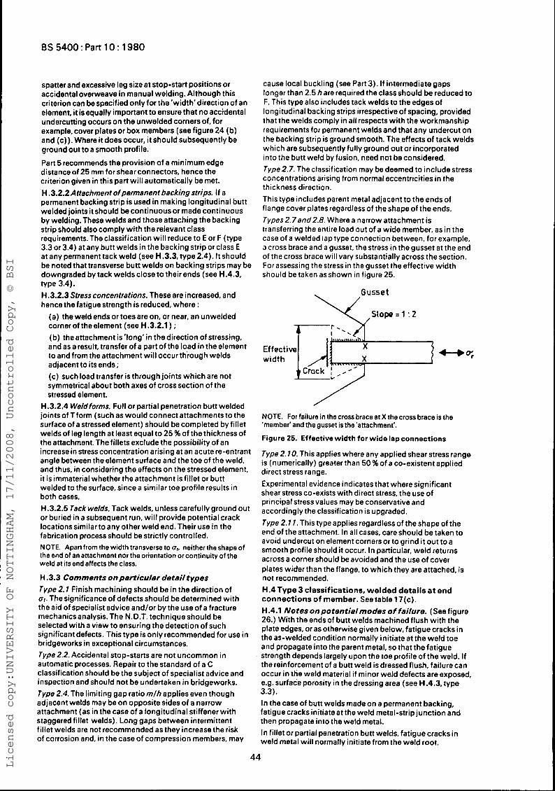
BS5400:PartlO: 1980
spatter and excessive leg size at stop-start positions or accidental overweave in manual welding. Although this criterion can be specified only for the'width' direction of an element, it is equally important to ensure that no accidental undercutting occurs on the unwelded corners of, for example, cover plates or box members (see figure 24 (b) and (c)). Whereit does occur, it shouldsubsequently be ground out to a smooth profile.
Part 5 recommends the provision of a minimum edge distance of 25 mm forshear connectors, hence the criterion given in this part wi l l automatically be met. .H .3.2.2 Attachment ofpermanent backing strips. If a permanent backing strip is used in making longitudinal butt weldedjointsitshould becontinuousor made continuous by welding. These welds and those attaching the backing strip should also comply with the relevant class requirements. The classification will reduce to E or F (type 3.3 or 3.4) at any butt welds in the backing strip or class E at any permanent tack weld (see H.3.3. type 2.4). It should be noted that transverse butt welds on backing strips may be downgraded by tack welds close to their ends (see H.4.3, type 3.4). H .3.2.3 Stress concentrations. These are increased, and hence the fatigue strength is reduced, where :
(a) the weld ends or toes are on, or near, an unwelded corner of theelement (see H.3.2.1) ; (b) the attachment is 'long' in the direction of stressing, and as a result, transfer of a part of the load in the element to and from the attachment will occur through welds adjacent to its ends ; (c) such load transfer is through joints which are not symmetrical about both axes of cross section of the stressed element.
H.3.2.4 Weldforms. Full or partial penetration butt welded jointsof Tform (such as would connect attachmentsto the surface of a stressed element) should be completed by fillet welds of leg length at least equal to 25 %of the thickness of the attachment. The fillets exclude the possibility of an increase in stress concentration arising at an acute re-entrant angle between the element surface and the toe of the weld, and thus, in considering the effects on the stressed element, it is immaterial whether the attachment is fillet or butt welded to the surface, since a similar toe profile results in both cases. H.3.2.5 Tack welds. Tack welds, unless carefully ground out or buried in a subsequent run, wi l l provide potential crack locationssimilar to any other weld end. Their use in the fabrication process should be strictly controlled. NOTE. Apart from the width transverse to U,, neither the shape of the end of an attachment nor the orientation or continuity of the weld at itsend affects the class.
H .3.3 Comments onparticular detail types Type 2. I Finish machining should be in the direction of Or. The significance of defects should be determined with the aid of specialist advice and/or by the use of a fracture mechanicsanalysis. The N.D.T. technique should be selected with a view to ensuring the detection of such significant defects. This type is only recommended for use in bridgeworks in exceptional circumstances. Type 2.2. Accidental stop-starts are not uncommon in automatic processes. Repair to the standard of a C classification should be the subject of specialist advice and inspection and should not be undertaken in bridgeworks. Type 2.4. The limiting gap ratio m / h applies even though adjacent welds may be on opposite sides of a narrow attachment (as in the case of a longitudinal stiffener with staggered fillet welds). Long gaps between intermittent fillet welds are not recommended as they increase the risk of corrosion and, in the caseof compression members, may
cause local buckling (see Part 3). If intermediategaps longer than 2.5 hare required the class should be reduced to F. This type also includes tack welds to the edges of longitudinal backing strips irrespective of spacing, provided that the welds comply in all respects with the workmanship requirements for permanent weldsand that any undercut on the backing strip is ground smooth. The effects of tack welds which are subsequently fully ground out or incorporated into the butt weld by fusion, need not be considered. Type 2.7. The classification may be deemed to include stress concentrations arising trom normal eccentricities in the thickness direction. This type includes parent metal adjacent to the ends of flange cover plates regardless of the shape of the ends. Types2.7and2.8. Where a narrow attachment is transferring the entire load out of a wide member, as in the case of a welded lap type connection between, for example, J cross brace and a gusset, the stress in the gusset at the end of the cross brace will vary substantially across the section. For assessing the stress in the gusset the effective width should be taken as shown in figure 25.
NOTE. For failure in the cross brace at X the cross brace is the 'member' and the gusset is the'attachment'.
Figure 25. Effective width for wide lap connections
Type 2.70. This applies where any applied shear stress range is (numerically) greater than 50 % of a co-existent applied direct stress range. Experimental evidence indicates that where significant shear stress co-exists with direct stress, the use of principal stress values may be conservative and accordingly the classification is upgraded. Type 2.7 1 . This type applies regardless of the shape of the end of the attachment. In al l cases, care should be taken to avoid undercut on element corners or to grind it out to a smooth profile should it occur. In particular, weld returns across a corner should be avoided and the use of cover plates wider than the flange, to which they are attached, is not recommended. H.4 Type 3 classifications, we lded detai ls a t end connections of member. Seetable 17(c). H.4.1 Notesonpotent ialmodes o f failure. (See figure 26.) With the ends of butt welds machined flush with the plate edges, or as otherwise given below, fatigue cracks in the as-welded condition normally initiate at the weld toe and propagate into the parent metal, so that the fatigue strength depends largely upon the toe profile of the weld. If the reinforcement of a butt weld is dressed flush, failure can occur in the weld material if minor weld defects are exposed, e.g. surface porosity in the dressing area (see H.4.3, type 3.3). In the case of butt welds made on a permanent backing, fatigue cracks initiate at the weld metal-strip junction and then propagate into the weld metal. In fillet or partial penetration butt welds, fatigue cracks in weld metal will normally initiate from the weld root.
44
Licensed copy:UNIVERSITY OF NOTTINGHAM, 17/11/2008, Uncontrolled Copy, © BSI
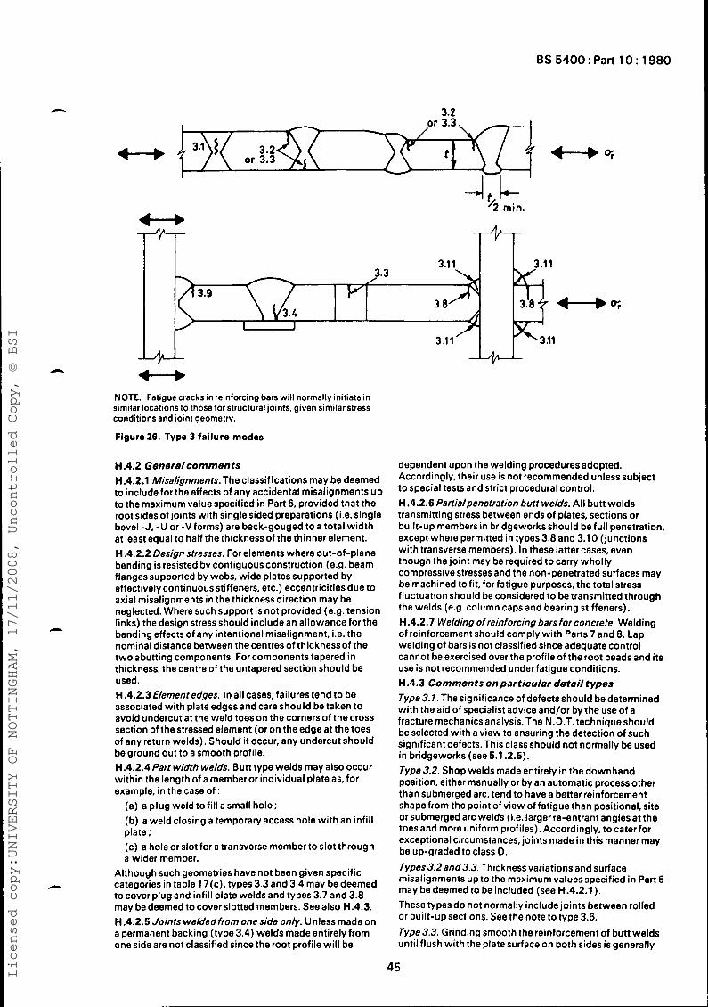
BS 5400 : Part 10 : 1980
3.2
3.2 - or 3.3
3.1 1 3.11 3.3
3.9
U i r e--+
NOTE. Fatigue cracks in reinforcing bars will normally initiate in similar locations to those for structural joints. given similar stress conditions and joint geometry.
Figure 26. Type 3 failure modes
H.4.2 Generalcomments H.4.2.1 Misalignments. The classifications may be deemed to include for the effects of any accidental misalignments up to the maximum value specified in Part 6, provided that the root sides of joints with single sided preparations (i.e. single bevel -J, -U or -V forms) are back-gouged to a total width at least equal to half the thickness of the thinner element. H.4.2.2 Design stresses. For elements where out-of-plane bending is resisted by contiguous construction (e.g. beam flanges supported by webs, wide plates supported by effectively continuous stiffeners, etc.) eccentricities due to axial misalignments in the thickness direction may be neglected. Wheresuch support is not provided (e.g. tension links) the design stress should include an allowance for the bending effects of any intentional misalignment, i.e. the nominal distance between the centres of thicknessof the two abutting components. For components tapered in thickness, the centre of the untapered section should be used. H.4.2.3Elernentedges. In allcases,failures tend to be associated with plate edgesand careshould be taken to avoid undercut at the weld toes on the corners of the cross section of the stressed element (or on the edge at the toes of any return welds). Should it occur, any undercut should be ground out to a smooth profile. H.4.2.4 Part width welds. Bun type welds may also occur within the length of a member or individual plate as, for example, in the case of :
(a) a plug weld to fill a small hole; (b) a weld closing a temporaryaccess hole with an infill plate ; (c) a hole or slot for a transverse member to slot through a wider member.
Although such geometries have not been given specific categories in table 17(c), types 3.3 and 3.4 may be deemed to cover plug and infill plate welds and types 3.7 and 3.8 may be deemed to cover sloned members. See also H.4.3. H.4.2.5 Joints weldedfrorn one side only. Unless made on a permanent backing (type 3.4) welds made entirely from one side are not classified since the root profile wi l l be
dependent upon the welding procedures adopted. Accordingly, their use is not recommended unless subject to special tests and strict procedural control. H .4.2.6 Partialpenetration butt welds. All butt welds transmitting stress between ends of plates, sections or built-up members in bridgeworks should be full penetration, except,where permitted in types 3.8 and 3.1 0 (junctions with transverse members). In these laner cases, even though the joint may be required to carry wholly compressive stresses and the non-penetrated surfaces may be machined to fit, for fatigue purposes, the total stress fluctuation should be considered to be transmitted through the welds (e.g. column caps and bearing stiffeners). H -4.2.7 Welding of reinforcing bars for concrete. Welding of reinforcement should comply with Parts 7 and 8. Lap welding of bars is not classified since adequate control cannot be exercised over the profile of the root beads and its use is not recommended under fatigue conditions. H .4.3 Comments on particular detail types Type 3.7. The significance of defects should be determined with the aid of specialist advice and/or by the use of a fracture mechanics analysis. The N.D.T. technique should be selected with a view to ensuring the detection of such significant defects. This class should not normally be used in bridgeworks (see 5.1.2.5). Type 3.2. Shop welds made entirely in the downhand position, either manually or by an automatic process other than submerged arc, tend to have a better reinforcement shape from the point of view of fatigue than positional. site or submerged arc welds (i.e. larger re-entrant angles at the toes and more uniform profiles). Accordingly, to cater for exceptional circumstances, joints made in this manner may be up-graded to class D. Types3.2and3.3. Thickness variations and surface misalignments up to the maximum valuesspecified in Part 6 may be deemed to be included (see H.4.2.1). These types do not normally include joints between rolled or built-up sections. See the note to type 3.6. Type 3.3. Grinding smooth the reinforcement of butt welds until flush with the plate surface on both sides is generally
45 Licensed copy:UNIVERSITY OF NOTTINGHAM, 17/11/2008, Uncontrolled Copy, © BSI
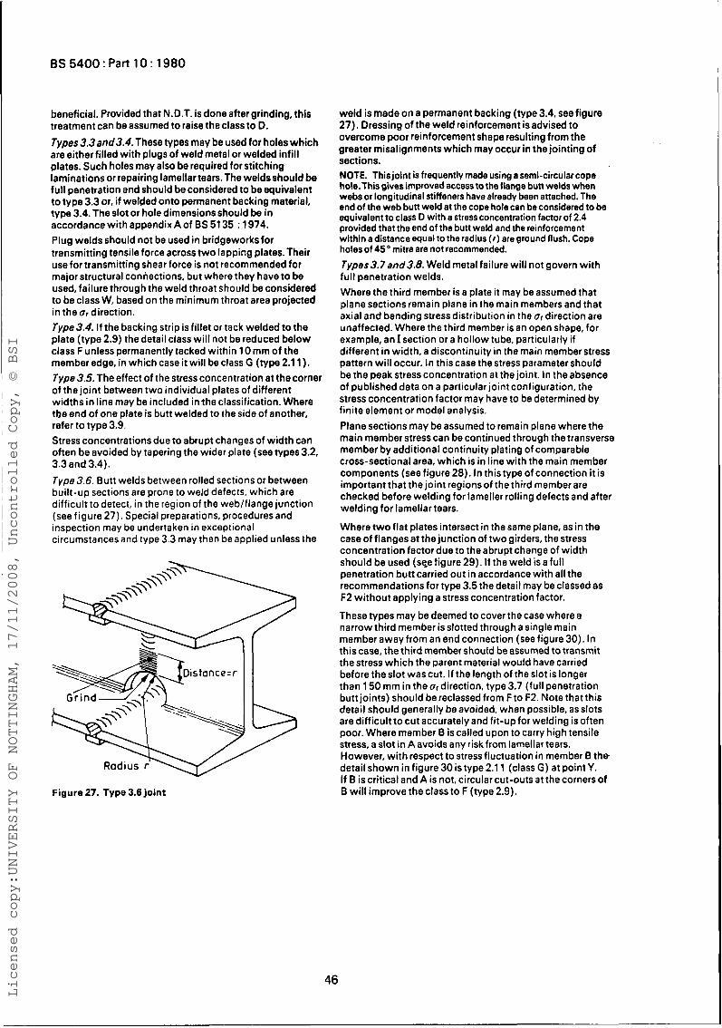
BS 5400 : Part 10 : 1980
beneficial. Provided that N.D.T. is done after grinding, this treatment can be assumed to raise the class to D.
Types 3.3 and3.4. These types may be used for holes which are either filled with plugs of weld metal or welded infill plates. Such holes may also be required for stitching laminations or repairing lamellar tears. The welds should be full penetration and should be considered to be equivalent to type 3.3 or, if welded onto permanent backing material, type 3.4. The slot or hole dimensions should be in accordance with appendix A of BS 51 35 : 1974. Plug welds should not be used in bridgeworks for transmitting tensile force across two lapping plates. Their use for transmitting shear force is not recommended for major structural connections, but where they have to be used, failure through the weld throat should be considered to be class W, based on the minimum throat area projected in the or direction. Type 3.4. If the backing strip is fillet or tack welded to the plate (type 2.9) the detail class wil l not be reduced below class F unless permanently tacked within 10 mm of the member edge, in which case i t will be class G (type 2.1 1). Type 3.5. The effect of the stress concentration at thecorner of the joint between two individual plates of different widths in line may be included in the classification. Where the end of one plate is butt welded to the side of another, refer to type 3.9. Stress concentrations due to abrupt changes of width can often be avoided by tapering the wider plate (see types 3.2, 3.3 and 3.4). Type 3.6. Butt welds between rolled sections or between built-up sections are prone to weld defects, which are difficult to detect, in the region of the web/flange junction (see f igure 27). Special preparations, procedures and inspection may be undertaken in exceptional circumstances and type 3.3 may then be applied unless the
Figure 27. Type 3.8 joint
weld is made on a permanent backing (type 3.4, see figure 27). Dressing of the weld reinforcement isadvised to overcome poor reinforcement shape resulting from the greater misalignments which may occur in the jointing of sect ions. NOTE. This joint is frequently made using a semi-circular cope hole.Thisgives improved access to the flange butt welds when webs or longitudinal stiffeners have already been attached. The end of the web butt weld at the cope hole can be considered to be equivalent to class D with a stress concentration factor of 2.4 provided that the end of the butt weld and the reinforcement within a distance equal to the radius ( I ) are ground flush. Cope holes of 45 O mitre are not recommended. Types3.7and3.8. Weld metal failure will not govern with full penetration welds. Where the third member is a plate it may be assumed that plane sections remain plane in the main members and that axial and bending stress distribution in the or direction are unaffected. Where the third member is an open shape, for example, an I section or a hollow tube, particularly i f different in width, a discontinuity in the main memberstress pattern wil l occur. In this case the stress parameter should be the peak stress Concentration at the joint. In theabsence of published data on a particular joint configuration, the stress concentration factor may have to be determined by finite element or model analysis. Plane sections may be assumed to remain plane where the main member stress can be continued through the transverse member by additional continuity plating of comparable cross-sectional area, which is in line with the main member components (see figure 28). In thistypeof connection it is important that the joint regions of the third member are checked before welding for lameller rolling defects and after welding for lamellar tears.
Where two flat plates intersect in the same plane, as in the case of flanges at the junction of two girders, the stress concentration factor due to the abrupt change of width should be used (see figure 29). I f the weld is a full penetration butt carried out in accordance with all the recommendations for type 3.5 the detail may be classed as F2 without applying a stress concentration factor.
These types may be deemed to cover the case where a narrow third member is slotted through a single main member away from an end connection (see figure 30). In thiscase, the third member should be assumed to transmit the stress which the parent material would have carried before the slot was cut. If the length of the slot is longer than 150 mm in the ar direction. type 3.7 (full penetration buttjoints) should be reclassed from F to F2. Note thatthis detail should generally be avoided, when possible, as slots are difficult to cut accurately and fit-up for welding is often poor. Where member B iscalled upon to carry high tensile stress, a slot in A avoids any risk from lamellar tears. However, with respect to stress fluctuation in member B the detail shown in figure 30 is type 2.1 1 (class G) at point Y. If B is critical and A is not, circular cut-outs at the corners of B will improve the class to F (type 2.9).
46
Licensed copy:UNIVERSITY OF NOTTINGHAM, 17/11/2008, Uncontrolled Copy, © BSI
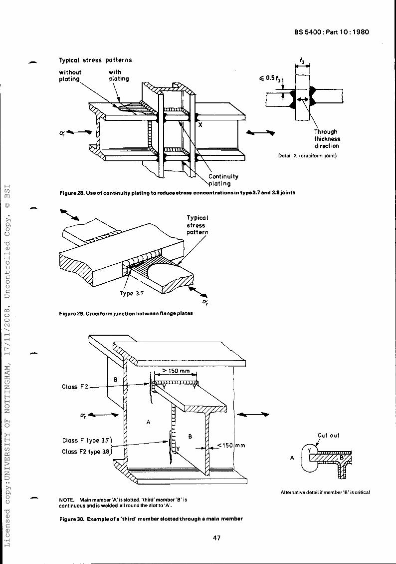
A Typical stress patterns
thickness direct ion
Detail X (cruciform joint)
\pia t i n g Figure28. Useof continuity plating to reducestress concentrations in type3.7 and 3.8 joints
n
0; Figure29. Cruciform junction between flange plates
Class F type 3.7
NOTE. Main rnernber'A issloned, 'third' rnernber'8' is continuous and is welded all round the slot to'A.
n
Figure30. Example of a'third' member slotted through a main member
47
A
cut out
Alternative detail if member '8' is critical
Licensed copy:UNIVERSITY OF NOTTINGHAM, 17/11/2008, Uncontrolled Copy, © BSI
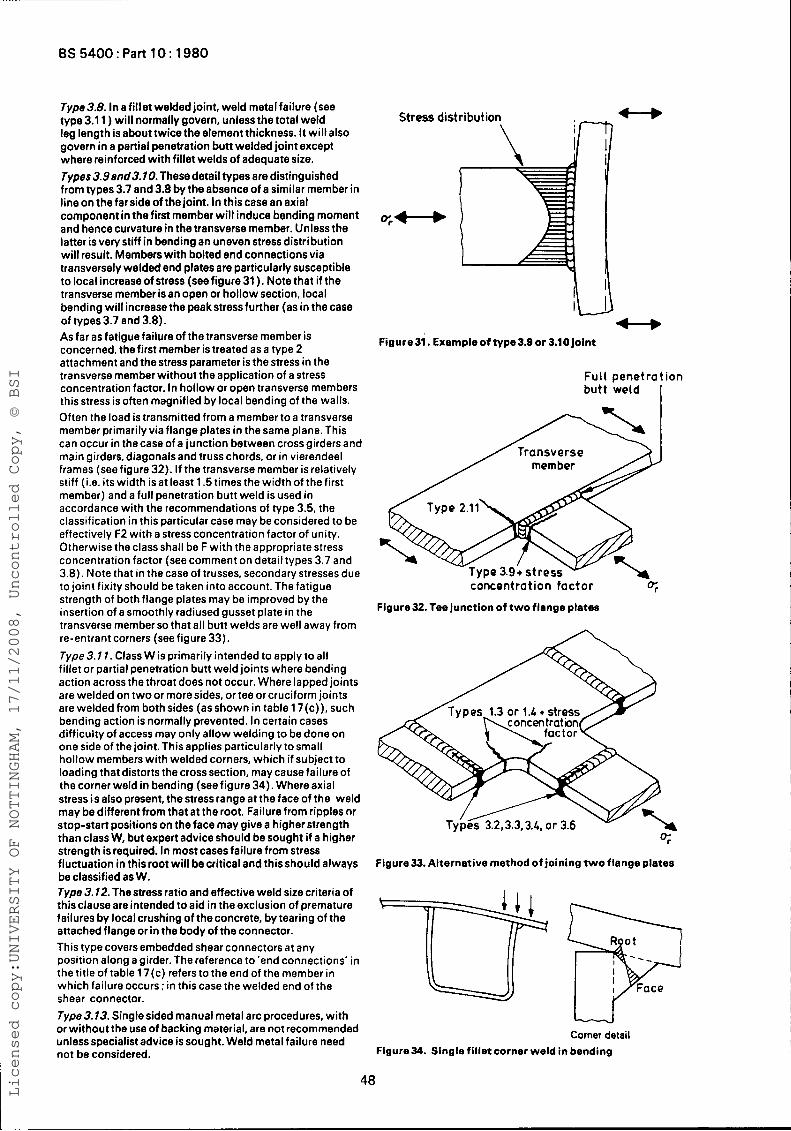
BS 5400:Part 10: 1980
Type3.8. In afillet welded joint, weld metal failure (see type 3.1 1 ) wil l normally govern, unless the total weld leg length is about twice the element thickness. It wilt also govern in a partial penetration butt welded joint except where reinforced with fillet welds of adequate size. Types3.9end3.tO.Thesedetail types are distinguished from types 3.7 and 3.8 by the absence of a similar member in line on the far side of the joint. In this case an axial component in the first member wil l induce bending moment and hence curvature in the transverse member. Unless the latter is very stiff in bending an uneven stress distribution will result. Members with bolted end connections via transversely welded end plates are particularly susceptible to localincreaseofstress (seefigure31). Notethat if the transverse member is an open or hollow section, local bending wil l increase the peakstress further (as in the case of types 3.7 and 3.8). As far as fatigue failure of the transverse member is concerned, the first member is treated as a type 2 attachment and thestress parameter is the stress in the transverse member without the application of a stress concentration factor. In hollow or open transverse members this stress is often magnified by local bending of the walls. Often the load is transmitted from a member to a transverse member primarily via flange plates in the same plane. This can occur in the case of a junction between cross girders and main girders, diagonals and truss chords, or in vierendeel frames (see figure 32). If the transverse member is relatively stiff (i.e. its width isat least 1.5 times the width of the first member) and a full penetration butt weld is used in accordance with the recommendations ot type 3.5, the classification in this particular case may be considered to be eftectively F2 with a stress concentration factor of unity. Otherwise the class shall be F with the appropriate stress concentration factor (see comment on detail types 3.7 and 3.8). Note that in the case of trusses, secondary stresses due to joint fixity should be taken into account. The fatigue strength of both flange plates may be improved by the insertion of a smoothly radiused gusset plate in the transverse member so that all butt welds are well away from re-entrant corners (see figure 33). Type3.11. Class W is primarily intended to apply to all fillet or partial penetration butt weld joints where bending action across the throat does not occur. Where lapped joints are welded on two or more sides, or tee or cruciform joints are welded from both sides (asshown in table 17(c)), such bending action is normally prevented. In certain cases difficulty of access may only allow welding to be done on one side of the joint. This applies particularly to small hollow members with welded corners, which if subject to loading that distorts the cross section, may cause failure of the corner weld in bending (see figure 34). Whereaxial stress i s also present, the stress range at the face of the weld may be different from that at the root. Failure from ripples or stop-start positions on the face may give a higher strength than class W, but expert advice should be sought if a higher strength is required. In most cases failure from stress fluctuation in this root wi l l be critical and thisshould always be classified as W. Type3.12.Thestressratioand effective weld sizecriteria of this clause are intended to aid in the exclusion of premature failures by local crushing of the concrete, by tearing of the attached flange or in the body of the connector. This type covers embedded shear connectors a t any position along a girder. The reference to 'end connections' in the title of table 17(c) refers to the end of the member in which failure occurs; in thiscase the welded end of the shear connector.
I - . . . . . . Type3.73. single Sided manual metal arc procedures, with or without the use of backing material, are not recommended unlessspecialist advice is sought. Weld metal failure need not be considered.
Stress distribution \ I if
0;-
4--b I Figure 31. Example o f type3.9 or 3.10 joint
Full pene t ra t i on bu t t weld I
concentrat ion fac to r ? Flgure32. Tee junction o f t w o flange plates
Figure 33. Alternative method o f joining t w o flange plates
Corner detail Figure=. Single fillet corner weld in bending
40
Licensed copy:UNIVERSITY OF NOTTINGHAM, 17/11/2008, Uncontrolled Copy, © BSI
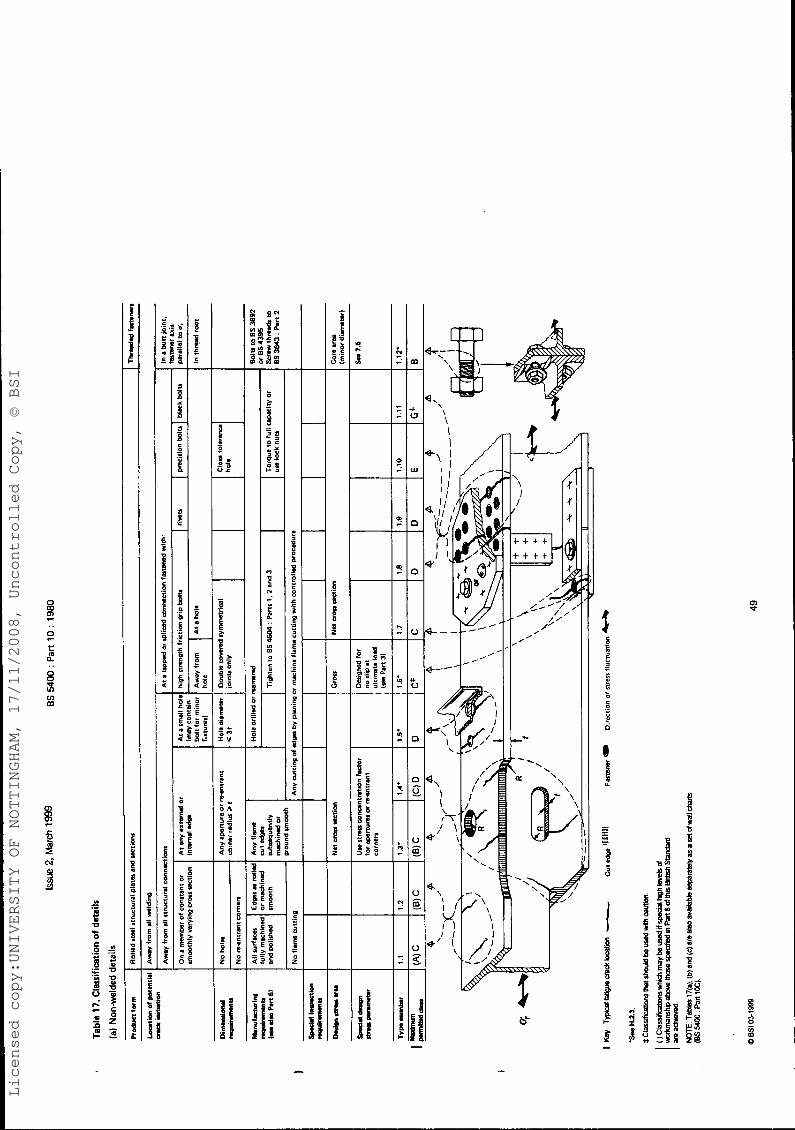
\ \
, , ,
P
Licensed copy:UNIVERSITY OF NOTTINGHAM, 17/11/2008, Uncontrolled Copy, © BSI
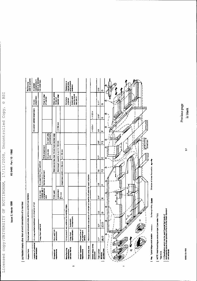
Licensed copy:UNIVERSITY OF NOTTINGHAM, 17/11/2008, Uncontrolled Copy, © BSI
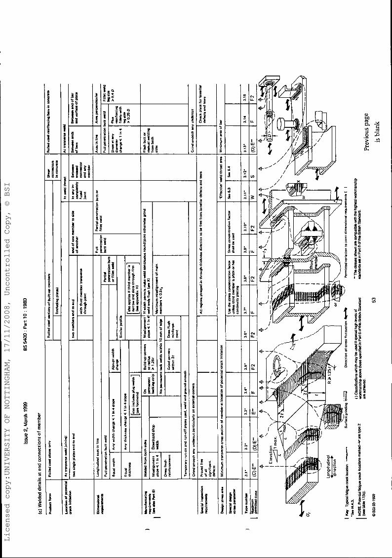
Licensed copy:UNIVERSITY OF NOTTINGHAM, 17/11/2008, Uncontrolled Copy, © BSI

n Standards publications referred to BS 1881 BS 3643 BS 3692 BS 419O 0s 4395 BS 4604 BS 5135 BS 5400
Methods of testing concrete IS0 metric screw threads I S 0 metric precision hexagon bolts, screws and nuts IS0 metric black hexagon bolts, screws and nuu High strength friction grip bolts and associated nuts and washers for structural engineering The use of high strength friction grip bolts in structural steelwork. Metric series Metal-arc welding of carbon and carbon manganese steels Stwl concrete and composite bridges
n
Licensed copy:UNIVERSITY OF NOTTINGHAM, 17/11/2008, Uncontrolled Copy, © BSI
issue 2, March 1999
This British Standard, having been prepared under the direction of the Civil Engineering and Building Structures Standards Committee, was published under the authority of the Executive Board and comes in to effect on 3 1 January 1980 8 BSI 03-1999 ISBN 0 580 10567 9
The fol lowing BSI references relate t o rhe work on this standard : Committee reference CSB/30 Draft for comment 74/13197 DC
BSI b the independant national body mponsible for preparing Bdtbh Standards. It presents the UK review on standards in Euro~e and at the htematiial level. It is hcorporeted by Royal Charter.
Rwloirlonr British Standards are updated by amendment or revision. Users of 8ritbh Standards should make sure that they possess the latest amendments or editions.
It is the anstant aim of BSI to improve the quality of our products and secv(ces. We would be grateful if anyone finding an inaccuracy or ambiguity while using this British Standard would inform the Seaetary d the responsible technical committee, the identity of which can be found on the inside front cover. Tel: 0181 996 9OOO; Fax: 0181 996 7400.
BSI offers members an individual updating service called PLUS which ensures that wbsaibers automatically receive the latest ediths of standards.
Buylng standards Orders for all BSI. international and foreign standards publications should be addressed to Customer Services. Tel: 0181 996 7000: Fax: 0181 996 7001.
BS 5400 : Part 10 : 1980 In response to orders far international standards, it is BSI policy to supply the BSI implementation of those that have been published as British Standards, unless othecwise requested.
Information on standards BSI provides a wide range of information on national, European and international standards through ita Libmy and its Technical Help to Exporters Service. Contact the Information Centre. Tel: 0181 996 7111: Fax: 0181 996 7048.
Subscribing members of BSI are kept up to date with standards developments and receive substantial discounts on the purchase price of standards. For details of these and other benefits contact Membership Administration. Tel: 0181 996 7002; Fax: 0181 996 7001.
Copyrlght Copyright subsists in all BSI publications. BSI also holds the copyright. in the UK. of the publications of the international standardization bodles. Except as permitted under the Copyright, Designs and Patents Act 1988 no extract may be reproduced, stored in a retrieval system or transmitted In any form or by any means - electronic, photocopying, recording or otherwise - without prior written permlssion from BSI.
This does not preclude the free use. in the course of implementing the standard, of necessary details such as symbols, and size, type 01 grade designations. If these detaik are to be used for any other purpose than implementation then the prior written permission of BSI must be obtained.
If permission is granted, the terms may include royalty payments or a licensing agreement. Details and advice can be obtained from the Copyright Manager. Tel: 0181 996 7070.
Committees responsible for this British Standard The Civil Engineering and Building Structures Standards Committee, under whose direction this British Standard war prepared, consists of representatives from the following Government departments and scientific and industrial organizations:
Association of Consulting Engineers Association of County Councils British Constructional Steelwork Association British Precart Concrete Federation Ltd. British Railways Board British Steel Industry Cement and Concrete Association Concrete Society Limited Constructional Steel Research and Development Organization Department of the Environment (Building Research Establishment)
Department o f the Environment (Transport and Road Research
Department of Transport Federation of Civil Engineering Contractors Greater London Council Institution of Civil Engineers Institution of Highway Engineers Institution of Municipal Engineers Institution of Structural Engineers London Transport Executive Ministry of Defence Sand and Gravel Association Lid. Scottish Development Department Welding Institute
Laboratory1
Amendments issued since publication
Amd. No. I Dateof issue I Text affected
9352 I March 1999 I Indicated by a sideline
British Standards InstiMion a 3 8 9 Chiswick High Road London W4 4AL - Telephone 0181 996 9OOO Fax 0181 996 7400
Licensed copy:UNIVERSITY OF NOTTINGHAM, 17/11/2008, Uncontrolled Copy, © BSI
![FATIGUE CLASSIFICATION OF WELDED JOINTS IN ...loading given in the UK bridge design code, BS 5400 part 10 [British Standards Institution, 1980] with stresses and fatigue classification](https://img.pdfslide.us/doc/110x75/5e66df2c423ec955dc042e62/fatigue-classification-of-welded-joints-in-loading-given-in-the-uk-bridge-design.jpg)