Stickies (hakon) 1 Thu, Apr 24, 2003

A BEGINNER’S GUIDE

TO THE

BRUKER AXS PACKand other noble time wasters

(A never-finished beta test version 4.0)

Prepared by Dejan Poleti with help from Tonči Balić-Žunić, Håkon Hope

and Ljiljana Karanović

©, ®, ™ and other possible and impossible rights belong exclusively to the authorsand GEOLOGISK INSTITUT, Københavns Universitet

This guide is mainly devoted to the instrument control and data acquisition program SMART V5.054.

However, some useful (?) comments about other Bruker programsRECIPROCAL LATTICE DISPLAY PROGRAM V3.0,

ASTRO V5.007, COSMO NT V1.42, SAINT V6.28A,

SHELXTL V5.1, XPREP V6.13and

SADABS V2.07are also included.

Copenhagen/Belgrade, 2003

I

A SHORT HISTORICAL SURVEY

The very first, shorter version of this text was written in the summer of 2000 during our(D. P. and Lj. K.) three-month visit to the Geological Institute, University of Copenhagen,Denmark. We suppose some readers wonder about our motivation to prepare the Guide? Nosecrets or urban legends, no dream appearances or touch of destiny! It was indeed necessaryto orient ourselves and to organize our minds when we for the first time faced a Bruker(Nicolet, Syntex, Simens, Bruker Nonius) AXS four-circle diffractometer equipped with a 1000 KCCD detector and a lot of its technical documentation, unjustly referred to as “Manuals.”

For almost one year the first version of our Guide was in use only in Copenhagen andParis (École Centrale). Readers, mainly beginners, like we were in ancient times three yearsago, described the document as very helpful and much better than the original documentation.No doubt about it, they can be judged guilty for putting that foolish idea into our heads. Thechallenge was big and we finally decided to offer the Guide to all users. The revised text(containing many new recommendations and description of the meanwhile installed version6.02a of SAINT+) was prepared during the summer of 2001; in September about 70 copieswere distributed worldwide as version 2.0.

Once again, the resonance was excellent, but the number of suggestions and remarkswas lower than we expected. (Very likely, the term “beginners” in the title repelled someexperienced users, and kept them from reading the text.) However, three members of ourcrystallographic and Bruker users community made great and un-selfish efforts to improve thecontent of the Guide. They are: Dr. Håkon Hope (Department of Chemistry, University ofCalifornia, Davis, USA), Dr. Gene Carpenter (Department of Chemistry, Brown University,Providence, USA) and Dr. James Ibers (Department of Chemistry, Northwestern University,Evanston, USA).

Dr. Hope edited the text in order to bring it closer to standard English. He also made theGuide more universal by writing completely new sections with a description of the Brukerthree-circle platform diffractometer with the video camera. In comparison to these twocontributions, most of the numerous other interventions and suggestions were smaller and willnot be explicitly mentioned here. Still, they were important, and we are grateful for havingreceived them.

Dr. Carpenter was kind enough to provide us with his instructions for using SADABS, tosend several MultiRun scan examples and to give many very useful suggestions.

Dr. Ibers informed us about practices in his laboratory and donated a few tips on how toperform data collection, integration and absorption correction in order to get better results.

Finally, on a suggestion from Dr. Hope, the paper size of the document has been set to acombination of Letter (US) length and A4 (European) width. Now all readers should be able toprint the Guide without any tedious reformatting (but this was only briefly tested for USstandard, 8.5¥11 inch paper). Nevertheless, the paging has been optimized for HP1000LaserJet (600 dpi). If you do not know what this means, see Post Scriptum at the very end ofthe Guide. For printing on A4 paper aesthetic reasons suggest you set (File > Page Setup…)top margin at 3.25 cm and paper height at 28.69 cm. Of course, some other options exist,including, for example, an entire reformatting while you wait for data collection to finish.

In some way Dr. Hope, Dr. Carpenter and Dr. Ibers are liable for the appearance ofversion 3.0, which was distributed in about 130 copies in June of 2002.

Meantime, several new programs or new versions have been released, and GeorgeSheldrick was so benevolent as to send a lot of comments and recommendations, which havebeen included in version 4.0. Personally, we have accumulated more experience and haveperformed several studies on data integration and absorption correction strategies. Theseresults are partially presented in this version as a collection of new instructions andrecommendations. Once again, Dr. Hope was so kind to edit the complete text, making manyimprovements and some new suggestions.

II

Starting from version 4.0, examples of SAINT output files prepared in landscape format(with good reason) are distributed as a separate package called “An Extract from SAINT outputfiles.” We believe this change will make the primary text more compact and easily readable, andthe examples should be more useful.

As you see, many crystallographers contributed to this text and we are very indebted tothem. But we don’t run away from our responsibility – all suggestions, comments, remarks and(why not?) praise should be sent to the signed authors. Share your knowledge with the rest ofthe crystallographic community! You should keep in mind that a final version of the Guide has tobe at least twice as heavy as the Bruker materials.

At the suggestion of several readers we have decided also to prepare the Guide as a.pdf file and this will be available soon.

Belgrade/Copenhagen, Jun 2003 The Authors

P.S. Very likely major updates of SMART, SAINT and SADABS (so-called TWINABS) havebeen released recently, though we have not seen the programs yet (but visit the web sitehttp://128.104.70.72/SHARE1/WWW/Meeting_2003/Presentations.htm with user name: brukerand password: elements 35, 92 and 36 (case sensitive). The new versions will integrate andscale data from twinned and incommensurate structures.

I

PRELIMINARY (BUT VERY IMPORTANT) NOTES

It is assumed that you are familiar with the Windows NT operating system.It is also important to know something about the good, old DOS. Bruker pack is a counter-intuitive mixture of both operating systems prepared in a very fashionable, patchwork style.Since the above-mentioned programs are not connected in any useful way, you should be

prepared for various troubles, especially with project management and file manipulation, aswell as with limited sizes of DOS (and other) windows.

Have fun!

Many chapters of this document can be used as a checklist! Some documents given in theAppendix can be printed separately and used as a reminder. “Crystal Identity Card” is of

special importance here. If you fill in this form regularly, with a lot of good luck all necessarydata will be kept together when the crystal structure determination is finished.

Do not be confused, although you probably will be.1 Some operations can be done in anidentical or very similar manner starting from different menu commands. Obviously Bruker’sstaff prefers to have a lot of menu items, or, perhaps their programmers were fascinated byautomation. However, crystallography is NOT, and will NEVER be brainless, routine

work! Therefore, we favor better control, which means step-by-step operationwhenever possible.

Be careful! Think!Do not trust your memory; keep your laboratory notebook up to date with as much detail as

possible. This is of great importance for your present, future and especially past work.Remember the Chinese saying: “Faint ink is better than the best memory.”

Note that some data, such as file or directory names, are laboratory and/or user specific.They are usually listed for our laboratory in Copenhagen or for Dr. Hope’s laboratory in Davis.Some other details could also depend on practice and standards in your laboratory, as well ason laws in your country. Finally, the proper strategy strongly depends on properties of

the crystals under study. This is sometimes, but not always mentioned in the text. Thismanual should not be a substitute for thorough discussions with experienced

crystallographers and your system administrator.

Disclaimer: Well, it is not reasonable to expect that we can go farther than Bruker...Therefore, the authors shall not be liable for errors ... nor for damages ... nor for... nor for... Insimple words: the use of this Guide is at your own risk. Examples given in figures andcomputer outputs may not represent the best solution for your problem and should not be usedwithout a grain (or a lot) of critical thinking. After all, please note that we payconsiderable attention to environmental problems. We recycle X-rays wheneverand wherever possible!

1 So what if you are? Who has never been confused by a computer program?

II

V

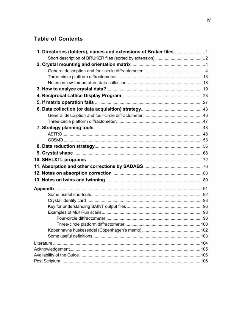
Table of Contents

1. Directories (folders), names and extensions of Bruker files ..........................1

Short description of BRUKER files (sorted by extension) ..........................................2

2. Crystal mounting and orientation matrix ..............................................................4

General description and four-circle diffractometer ....................................................4Three-circle platform diffractometer.........................................................................13Notes on low-temperature data collection................................................................18

3. How to analyze crystal data?.................................................................................19

4. Reciprocal Lattice Display Program ....................................................................23

5. If matrix operation fails ... .......................................................................................27

6. Data collection (or data acquisition) strategy....................................................43

General description and four-circle diffractometer ..................................................43Three-circle platform diffractometer.........................................................................47

7. Strategy planning tools............................................................................................48

ASTRO......................................................................................................................48COSMO .....................................................................................................................53

8. Data reduction strategy...........................................................................................56

9. Crystal shape.............................................................................................................68

10. SHELXTL programs..................................................................................................72

11. Absorption and other corrections by SADABS..................................................76

12. Notes on absorption correction ...........................................................................83

13. Notes on twins and twinning..................................................................................89

Appendix ............................................................................................................................91Some useful shortcuts..............................................................................................92Crystal identity card..................................................................................................93Key for understanding SAINT output files ................................................................96Examples of MultiRun scans.....................................................................................98

Four-circle diffractometer..................................................................................98Three-circle platform diffractometer................................................................100

Københavns huskeseddel (Copenhagen’s memo) .................................................102Some useful definitions...........................................................................................103

Literature ............................................................................................................................104Acknowledgement..............................................................................................................105Availability of the Guide......................................................................................................106Post Scriptum......................................................................................................................106

I

1

1. DIRECTORIES (folders), NAMES AND EXTENSIONS OF BRUKERFILES

The files used by a project normally reside in one of three directories: working, data orcalibration directory.

The calibration directory contains the detector parameter file and different calibrationfiles. This directory is shared by all projects. For everyday work it is important to remember thatall measured dark-current files (._dk, see below) are located in this directory, from where theycan be reused. The other files in the calibration directory are used automatically and rarelyrequire updating, or need no updating at all.

The location of files in the other two directories could be slightly confusing.The working directory contains files written during crystal orientation and unit cell

determination (that is, when ACQUIRE > Matrix, ACQUIRE > Rotation, CRYSTAL > Unit Cell, etc.commands are run).

The data directory is the destination for frames collected during scan runs, i.e. duringdata collection performed by ACQUIRE > MultiRun ...> Hemisphere, or ... > Quadrant. Thisdirectory could be on a networked, off-line computer, while the working directory is always onthe computer that is directly connected to the instrument. Of course, both directories can belocated on the same computer. After some unpleasant experiences with network breakdownsour current practice is: measure everything on the directly connected computer, transfer dataafterwards to where you want to work on them.

The working and data directories also include smart.ini (or smartdef.ini) and specificcalibration files used for a given project.

As usual, file names consist of two parts: jobname and extension, that isname.ext.

By default they follow the well-known and very old DOS 8.3 convention (but other setups arealso possible in EDIT > Config dialogue box, Fig. 2.3, see SMART manual, p. 6-3.).

The jobname is freely chosen by the operator to describe the crystal or project. Thecombination of crystal name and crystal number forms Project name, which must be unique. It isstored in the ASCII project database file administrator.prj (located in directoryc:\frames\Projects\ or d:\frames\Projects\). Note: During the installation of SAINT this file may benamed other than adminstrator.prj (consult system administrator if necessary).

During data collection the Bruker system will add some numbers to the file-name field. Forinstance, the names of output frames could be: name1.ext, name2.ext, etc., whereunderscored numbers are automatically set by the system.

The first number behind the jobname is the crystal number as set in the Projectdescription. (It is, of course, possible to use the same crystal more than once, or, on the otherhand, more crystals of the same kind can be used for a data collection.) As shown above, oneadditional number often appears in the name field. This number, just before the dot, is Run# andrepresents sets of data collected during MATRIX, MULTIRUN, etc. procedures.

The numbers in the extension are Frame#. Thus, name21.001, name21.002 ...name22.458, etc. show jobname, crystal 2, data sets 1 and 2, frames 001, 002 and 458,respectively. If the frame number is higher than 999 then letters a, b, etc. will appear in thatfield.

- If the letter m appears just before the dot (for example, namem.ext), it means that suchfile contains data merged from several different data sets.

2

- If the letter t appears just before the dot (for example, namet.ext), it means that such filecontains merged, decay-corrected results from the SAINT program.

- If the letter u appears just before the dot (for example, nameu.ext), it means that suchfile contains unsorted results.

Short description of BRUKER files (sorted by extension)

Extensions of the most important files are given in bold letters!2

.001, .002, etc. Files containing different measurement pictures, or so-called frames, prepared by

program SMART during data collection.bg_snap.000, bg_snap.001, etc.

Files (written by SAINT) containing a snapshot of the background calculated during theintegration.

.cif CIF, Crystallographic Information File prepared by the SHELXTL suite after the finalstage of structure refinement (see also .pcf). After editing, this file is suitable forsubmitting a paper to Acta Crystallographica and many other journals, or fordeposition in CCDC, ICSD and similar databases.

.edx, .edy, .edzFiles containing statistical results from program SAINT (if ‘Generate Diagnostic Plot

Files’ is checked). These files contain intensity deviation scatter plots showingintensity deviations vs. position and can be viewed using PLOTSO, SMART, SADIEor FRAMBO.

.exx, .eyy, .ezz, .exz, .eyz, .exiFiles containing statistical results from program SAINT (if ‘Generate Diagnostic Plot

Files’ is checked). These files contain positional deviation scatter plots showingpositional errors vs position and can be viewed using PLOTSO, SMART, SADIE orFRAMBO.

.fcf File containing structure factors in CIF format.

.ini Configuration file where initial parameters, as well as instrument and sample data arestored (e.g. smart.ini, smartdef.ini, saint.ini, saintCL.ini).

.ins Command (input) file for SHELX programs.

.hkl If you don’t know about this file you probably are not a crystallographer. Leave oursession immediately!

.lst File produced by SHELX programs and containing results of crystal structure solutionor refinement.

.p4p VERY IMPORTANT FILES! Parameter files containing crystal data, unit cell parameters,orientation matrix, reflection arrays, etc. The file is often updated with additionaldata during MATRIX operations and after data collection.

.pcf A part of CIF prepared by the XPREP program. This file contains crystal system, spacegroup, some experimental data, etc. in CIF format (see also .cif).

.prj A file (actually administrator.prj) containing Project names and located inc:\frames\Projects\ or d:\frames\Projects\ directories.

.prp Login (history) and results of program XPREP.

2 Some files are in binary format and you will probably never find a use for them.

3

.raw File containing reflections sorted as symmetry equivalents (after integration by SAINT).Contains practically all information about the reflections. The format of the raw fileis explained in SAINT+ help. See files INTEGRATEHELP.PDF orINTEGRATEHELP.HLP.

.rot Optional (but common) extension for a rotation picture obtained by ACQUIRE > Rotationor CRYSTAL > Evaluate commands in SMART.

.slm Script file.

._am Active mask, or active pixel mask, created from the initial background frame (programSAINT).

._dk Dark-current frame. An old dark-current frame file can be adequate for a MATRIXprocedure. However, it is highly advisable to collect a new dark-current correctionfile before data collection (see “Data Collection Strategy” below). These files areregularly located in c:\frames\ccd_1k folder. The dark-current frame used is alsoautomatically saved in the working and data directories.The usual convention in our laboratory is to give an eight-digit name in the formattimeyymmdd._dk. For example, 60000703._dk means: 60 seconds of backgroundcollection taken on 2000/07/03; 3M990722 means: 3 minutes dark frame collectedon 1999/07/22.

._br Brass plate image (a calibration file, forget it).

._ff Flood field image file (a calibration file, forget it).

._fl Flood table, flood-field correction or flood correction file. Similar to the dark-currentframe file, but containing pixel-by-pixel uniformity correction. Does not need to beupdated, so you can almost forget it. However, verify with the system administratoror some other experienced person that you are using the correct one.

._ib Initial background, providing the starting point for preliminary background refinement inprogram SAINT.

._if File containing table used to transform pixels from raw to corrected values(information only, forget it).

._it File containing table used to perform reverse transformation with respect to the ._if file(information only, forget it).

._ix File containing indexed fiducial spot positions for spatial correction. It does not need tobe updated. (See the note for ._fl files!)

._lg Log file (present only if login option is on).

._ls Intensity integration results (log file of SAINT run). If multiple runs have been integratedtogether, there is also a merged file with the name ending in m (see above).

._rb results of intensity integration done by SAINT > Integrate (for example, a filename1.001 will become name1._rb, etc.).

4

2. CRYSTAL MOUNTING and ORIENTATION MATRIX

General description and four-circle diffractometer

The work starts with mounting what we think is the best crystal in the batch we obtained(lucky girls and guys who work with or are themselves synthetic chemists, and can chooseamong a mass of good crystals), or what is the only available rubbish we have (in the case ofmineralogists or not so lucky synthetic chemists!). Then comes the moment of truth: apreliminary check on the diffractometer – the crystal will turn out to be something we just throwaway and choose another (for the above-mentioned lucky girls and guys...) or will offer us aglimpse into the problems that await us while trying to solve its structure.

In the old days some crystallographers would use film methods for this part of the crystalchecking before turning to measurements on a diffractometer. So why not spend an hour ortwo carefully examining the preliminary data before you start filling your computer withmegabytes of data collection? On the other hand, with the current instrument it is possible tostart data collection right away, and then by inspecting some tens of the first frames to decidewhether to proceed (and how) or not. The latter method is not something we wouldrecommend, and let it hereby be revealed that the authors of these lines are so old as to beeducated in that ancient era before the advent of personal computers when students were stilltaught to plan their experiments.

The selection of single crystals by well-documented trial and error methods will not bedescribed here. Drink enough to stop your hands from trembling, but not so much as to make itworse! (But note that some countries prohibit the operation of X-ray machines while under theinfluence of alcohol or some drugs.)

In our system the single crystal should not be larger than about 0.6-0.7 mm. The largestavailable collimator pinhole is 0.8 mm in diameter. As a rule, smaller crystals are preferable,especially if they contain heavy elements and absorption is significant. Recommendeddimension for sulfides and oxides of heavier elements is ca. 0.1 mm, for common silicates andoxides containing lighter elements 0.2-0.3 mm, for organics ca. 0.5 mm. In any event, an optimalcrystal dimension, t, can be calculated by the well-known relation t = 2/m, where m is the linearabsorption coefficient. (For organic and coordination compounds m usually lies between 0.1and 2 mm–1, for compounds containing heavier elements m is about 10 mm–1, while forcompounds with a high content of Tl, Pb or Bi it can reach 80 mm–1.) However, the formulagives too large size for most organic and many organometallic compounds (with no very heavyatoms) and too small size for highly-absorbing crystals.

From the results published recently by Rühl & Bolte (2000) follows that narrow (0.2 and 0.3mm) collimators should be avoided, since, with all other conditions kept constant, they give low-quality data and the worst R-indices. This can be attributed to the inhomogeneity of the collimatedbeam. The best results are obtained with a 0.5 mm collimator, but a 0.8 mm collimator yields verysimilar results.

It is interesting to emphasize that crystals much larger than the collimator pinhole can besuccessfully used for data collection; for example, if it is risky to cut a smaller piece (Görbitz, 1999;Rühl & Bolte, 2000). However, the greatest surprise was the conclusion that better results areobtained for larger crystals (Rühl & Bolte, 2000). It seems that the effect of a higher number ofscattering centers more than compensates for the negative influence of absorption. This is inaccordance with the authors’ belief that highly diffracting crystals would give good data under nearlyall experimental conditions, so the most important thing is to obtain strong reflections.

5

The reader must be warned here that low-diffracting and low-absorbing (m < 0.2 mm–1) organiccrystals with oxygen as the heaviest element (so-called “small organic molecules”) were used in theRühl & Bolte (2000) and Görbitz (1999) studies. (But we also confirmed their results using a verylarge crystal of one borate mineral with m ª 1.3 mm–1.) In contrast, in our laboratory sulfides of heavyelements with m typically over 40 mm–1 are often measured, and absorption correction usuallydecreases Rint by 2/3. With the transmission factor getting as low as 0.001 one usually does not usecrystals over 0.1 mm in diameter.

In a radical approach of Dr. Ibers (private communication) one should use the largest crystalcommensurate with the collimator pinhole. Of course, this could be recommended only if physicallymeaningful, face-indexed absorption correction can be applied.

The overall length of the glass fiber should be about 1.4 cm. 3 After mounting in the brasspin, the visible part of the fiber should be ca. 0.7 cm long. Mount the fiber properly (in linewith the brass pin axis) using wax. Fix the crystal by dipping the top of the fiber in glue(do not take too much of it!) and picking up the crystal. In order to minimize absorptioneffects it is advisable to fix the sample with its smallest surface attached to the top of thefiber, but not directly along the main axis. Mount the brass pin in the goniometer head.

!!! Do not forget to unlock the head! (Find three small screws; ask an experiencedperson if you are in doubt. But also see next paragraph.)It should be mentioned that in some laboratories beginners are not allowed to remove ormount goniometer heads, or to change the tension of the locking screws. In any event,always use both hands when you carry the goniometer head box. In other laboratoriesthe goniometer head is always left on the diffractometer. Locking tension is set forsmooth movement and stability, and is rarely adjusted. Only the mounting pin is moved.

You can cancel any diffractometer operation by pressing the Ctrl+Break or Esc keys. Inthe first case SMART will interrupt the run instantly. The second case gives a “smoothbreak”, meaning that the current operation will be finished.An interrupted MultiRun scan can be continued using ACQUIRE > Resume.

•fi Check diffractometer angles. If necessary set them to zero by running

GONIOM > Zero (or F10 shortcut),then confirm YES.Mount the goniometer head on the goniometer. Find a mark on the bottom part of thegoniometer head. In order to mount the head properly the mark should be away from you.(There is a secret slot on the base of goniometer head which should match the smallnipple on the screw base of the goniometer; but do not try to see the slot with yourcrystal mounted!)In order to have appropriate menu items you should switch to Level 2 in the LEVEL menu.During work, look at the bottom part of the SMART window. Sometimes it is possible tofind useful information there.

3 This set of instructions is appropriate for a four-circle diffractometer and room-temperature work only (but ourdiffractometer is not equipped with a low-temperature device).

6

••fi Define a New project with

CRYSTAL > New Project.Define the Project Name and type in all known data (Fig. 2.1).At least Crystal name, Crystal number, Working and Data directories must be defined. Ifyou leave Data directory blank, it will default to the Working directory. Do not worry toomuch, the remaining items can be filled in later with CRYSTAL > Edit Project. As statedpreviously, the combination of Crystal name and Crystal number must be unique. If it isnot, SMART will increment the crystal number. We strongly recommend that you use anew directory for each crystal. Otherwise, old data can be easily overwritten.Press Enter or click OK when you enter data and choose Small Molecule from the nextmenu.

Fig. 2.1. ‘Crystal > New Project’ and ‘Crystal > Edit Project’ dialogue box.

Note: It is also possible to use the present configuration and to enter your temporary databy the above-mentioned CRYSTAL > Edit Project command. However, we do notrecommend it, because in that case it will be easy to forget to define New Project later, orsome instrumental corrections could be out of date. A project can also be defined usingCRYSTAL > Copy Project and CRYSTAL > Config To Project commands. Once defined,the project can be activated using CRYSTAL > Switch To Project.

•fi Center crystal optically with

GONIOM > Optical (Ctrl+O shortcut)orCRYSTAL > Evaluate.The latter command automatically performs optical alignment and takes a rotation picture.For some slightly obscure reason, which we experts wish to keep to ourselves (but seePreliminary notes), it is better to use the first option.

!!! Do not forget to note crystal dimensions (maximum, intermediate and minimum) duringthe optical alignment operation.In any case a dialogue box appears with some pre-defined diffractometer angles. First ofall, check that they correspond to the goniometer used. (From time to time and for

7

unknown reasons SMART forgets the pre-defined base angles.4) For our P4 goniometerthey should be 2-theta = 0°, omega = 0°, phi = 60° and chi = –30° (or 330°). Then pressENTER and find the manual box on a sidewall of the diffractometer cage.When using the GONIOM > Optical command with default angles (marked A, B, C, and Don the manual box)5 one of the slides on the goniometer head is always perpendicular tothe viewing direction. The 180° rotation around phi when activating the AXIS PRINT buttonwhile keeping the same angular button depressed, is designed to adjust this slide, so thatthe crystal is well centered after repeated 180° rotations. Positions A+B and C+D arerotated to each other by 180° around chi (the first two hold the goniometer head pointingup, the latter two pointing down).For crystal centering we recommend the following procedure: Start with the Abutton depressed and activate the AXES PRINT button to drive the goniometer to thestarting position. Adjust the crystal both in the horizontal and the vertical directions (notethe appropriate drivers on the goniometer head). Then depress B followed by AXESPRINT. After this the crystal should be clearly visible (it is now in focus) so you canadjust it precisely in the horizontal direction. The extreme left and right points of thecrystal should be equidistant from the center of the microscope cross (keep thegraduated scale horizontal, it can be rotated by gently turning the microscope eyepiece –do not push the microscope sideways!). By repeating AXIS PRINT check the center point.If it exactly coincides with the vertical line of the crosshair, the crystals outermost pointsshould be equidistant from the center after the 180° rotation. If the crystal is now shiftedto one side, adjust it in the opposite direction for half of the displacement, and note theposition of the center of rotation. Repeat AXIS PRINT with B depressed until the crystalstays on the axis. Now depress A and do the final centering in this position (by repeatedrotations). Set the graduated scale (reticle) in the eyepiece vertical and finely adjust thevertical position of the crystal. Now depress C or D and activate AXIS PRINT. While thecrystal rotates to the new position you can check it through the microscope (it rotatesalmost through all possible positions).

!!! It can well happen that SMART will choose to rotate around chi so that the goniometerhead runs into the beam-stop mounted on the collimator (according to Murphy’s law italmost certainly will; see also footnote 4), although it could as well go the other way andavoid it. Do not loose YOUR head and with it your crystal, collimator, or centering of themicroscope by making some stupid panic move. Just gently push the beam-stop around,ahead of the racing goniometer head. It is easily moved, and the goniometer head coulddo it by itself without any damage, but we suggest you do it with a gentle touch of thehuman hand (here robots still cannot cope).Readjust the vertical position if necessary by switching between A (or B) and C (or D),and that’s it!

•fi If you prefer, it is possible to center the crystal without default positions. In that case use

GONIOM > Manual (Ctrl+M shortcut).Then press the desired axis button on the manual box and use the right-hand buttons(fast, slow, forward, or reverse) to get suitable angle positions. Be careful, think aboutcollision danger!

Tip: It is easier to measure a crystal in Manual than in Optical mode. It might be better to waitwith the precise determination of crystal dimensions until you believe the crystal issatisfactory (i.e. after the MATRIX operation).

4 SMART is not as smart as one could expect.5 The left-hand buttons on the manual control box are usually labelled with both letters and angles.

8

!!! After the crystal has been centered, lock the goniometer head slides and recheck thecrystal centering. Then press Esc to quit the operation. Close the doors, adjust until alllights are green, and press the ‘Reset’ button.

•fi Again set the diffractometer angles to zero (GONIOM > Zero or F10 shortcut). Confirm‘Yes.’

•fi If necessary, raise voltage and current to the desired values by

GONIOM > Generator.!!! Adjust the voltage first! Both parameters have to be increased in steps of 5 until the

normal values for our system, 40 kV and 35 (or 37) mA, have been reached (Mo tube).•fi Perform

GONIOM > Home Axis,which checks the calibrated position controls of the goniometer circles, so that thereported positions are exactly consistent.

!!! This command should be repeated four times, to home all four axes on the P4goniometer (however, since default values are listed sequentially, it is enough to pressEnter to advance to the next axis).

Fig. 2.2. ‘Acquire > Rotation’ dialogue box.

!!! Look at the pointers on the goniometer scales. They can easily get 1° away from zeroand Home Axis will not notice. If the pointers do not show 0°, use Manual mode andposition the goniometer circles close to zero. Then repeatGONIOM > Home Axis.

•fi Take a rotation photograph (rotation around phi) by

ACQUIRE > Rotation.Set the time if necessary (Fig. 2.2), but the shortest time is 72 seconds, and this value isa good choice if the crystal is not very small. (There is a conflict in the manual here, seepages 2-13, and it is not quite clear what is the shortest time allowed by the goniometerrotation speed.) Leave default values for the other parameters. Beware, rotationphotographs are not stored automatically, but must be saved using FILE > Save if youwish to keep them for documentation (a common extension for rotation photographs is.rot).Some characteristic rotation photographs are shown in Fig. 2.3. The intensities of spotscan give you an idea about the measurement time required for a frame; the number ofspots gives you an idea about how many frames to collect for the initial latticedetermination. (If you think you do not see anything in your rotation photograph, tryanother one with an exposure that is at least twice as long.)

9

a) b)

c) d)

Fig. 2.3. Examples of rotation photographs: a) a poly- and micro-crystalline sample,b) a polycrystalline sample containing several big and several small crystals, c) a good, singlecrystal sample, d) the same as c), but with photo converted to a film-like view. (Note that the

last picture is not produced in SMART, but by screen capture and further handling.)

After making a preliminary choice, also make a preliminary scan of 10 frames. Continueas follows:Open the ACQUIRE > Edit MultiRun menu and edit to get only one line:1 001 0 0 0 0 3 0.3 10 t(t should be your estimated exposure time per frame in seconds).After that, start ACQUIRE > MultiRun, give the name “Trial”, ”Test” or something like that(this would be the name of the frames) and press Enter. When the operation is finished,check the collected frames for appropriate exposure time. Maybe you are not quitesatisfied with the intensity of the spots and wish to increase the exposure time, orperhaps the spots are so intense and nice that you can use a shorter time. But do not gobelow 10 seconds per frame.If the spots tend to appear on only one, or at most two sequential frames, you have todecrease the step size called ‘Frame width’ in SMART. Increasing the step size to morethan 0.3° is not advisable, even if some spots continue through many frames. Afterchoosing the step size, make the following calculation:

N = 160 / [(number of spots) x (selected step size)].This gives you an estimate of the number of frames, N, needed for a good MATRIXoperation (see later). However, values lower than 20 or higher than 60 frames are notrecommended.

10

Also, check the crystal quality with the ANALYZE > Graph andANALYZE > Graph > Rocking commands described in the next chapter. They can revealsplitting of spots due to a fragmented or composite sample.

Tip: Your crystal is poor and yielded only a powder diffraction pattern (as in Fig. 2.3.a). Donot give up immediately. Use a vector cursor described in the next chapter to measurethe diameter of at least three of the most prominent circles, read d-values (in Ångström)to the right of the image and divide them by two. If any powder diffraction database is onhand, use these d-values to search through the base. Who knows, maybe the structurehas already been described, or unit cell parameters have been determined before, or youhave another example of isostructural compounds and isomorphous replacement, or …

Fig. 2.4. ‘EDIT > Config(uration)’ dialogue box.

••fi If the crystal is not discarded after the previous operation, the next step is acquisition ofan orientation matrix. Before that, invokeEDIT > Configand check the diffractometer configuration (Fig. 2.4). Input proper ‘Source kilovolts’ and‘Source milliamps’ values. Check with your system administrator that you have the correct‘Sample-detector distance’ and the correct ‘Direct beam X’ and ‘Direct beam Y’ center.Check also if the proper FloodFld (flood-field correction) and Spatial corrections are used.For our detector, at the bottom right in the SMART window both fields should contain thesame code, h423l17 (extensions are not visible). Be sure to have a Dark-field correctionof appropriate time (the same as you use for the exposures in Matrix). See description of._dk files in the beginning of this Guide. If necessary, load one from the c:\frames\ccd_1k(FILE > Load Dark), which has the most recent date.

•fi After that invoke

ACQUIRE > Matrix, or the equivalent CRYSTAL > Unit cell.These commands automatically collect three (short) series of scans at different startingangles, clear Reflection Array, invoke Threshold and store some collected spots into theArray, perform Autoindexing procedures, perform least-squares on the reduced primitivecell, determine the Bravais lattice, perform a least-squares refinement of the resulting unitcell, and finally write the new cell parameters into a .p4p file.

11

Choosing proper values in the corresponding dialogue box (Fig. 2.5) should be possibleby the checking procedure described above, but be sure that some skilledcrystallographer is on hand. In short, the values are:- ‘# Frames’ (number of frames) in a series preferably between 20 and 60,- ‘Frame Width’ preferably between 0.2 and 0.3°,- ‘Seconds/frame’ preferably from 10 to 60 s, but it could be even 180 s, for very small orpoorly diffracting crystals.- ‘Indexing HKL tolerance’ and ‘LS RLV tolerance’ should be 0.1 and 0.01, respectively,for expected excellent quality crystals, or 0.2 (no more than 0.25) and 0.02, respectively,for expected problematic cases.

Fig 2.5. ACQUIRE > Matrix dialogue box.

If you did not change ‘Job name’ (why should you?), the collected frames will be namedfrom matrix0.001 (matrix1.001, matrix2.001) to matrix0.xxx (matrix1.xxx, matrix2.xxx),where xxx is the number of frames in each series defined by the ‘# Frames’ argument.If the MATRIX operation finishes successfully, you will obtain initial cell parameters andother data required to perform data collection. In that case, the working directory containssmart.ini, three sets of matrix data, as well as the orientation matrix, unit cell parametersand other data needed in a proper matrix#.p4p file.

12

Tip: In collecting data for the preliminary cell determination and orientation matrix, instead ofMATRIX you can start with ACQUIRE > EditQuad(rant) and edit the field to get thefollowing lines:0 001 -28.00 -5.00 70.00 -110.00 2 .300 n t1 001 -28.00 -28.00 104.50 4.00 2 .300 n t2 001 -28.00 -28.00 -20.50 26.50 2 .300 n t3 001 28.00 28.00 9.50 -16.50 2 -.300 n t

where n is the number of frames in each series (40 is usually enough) and t is theexposure per frame estimated as described above. Then use ACQUIRE > Quadrant withjobname “MATRIX” followed by Crystal > Redtn Cell in an attempt to determine the cellautomatically. A general characteristic of this approach is that these four series of shortscans are directed approximately toward tetrahedral faces (with mutual angles of ca.109°) and cover, at least partially, the whole reciprocal space (not only a hemisphere).So you could expect easier determination of the orientation matrix, faster indexing, bettercell parameters, much less parameter correlation and even refinement of crystaltranslations. (Some other combinations of angles could be suitable too.) Of course, wedo not expect a beginner to try this with her first (or second, or third, or even fourth)crystal.

If the attempt to find unit cell parameters fails, ... then you can:a) Choose to spend your time with something easier than crystallography, orb) Find the chapter “If Matrix operation fails ...” somewhere below, orc) Ignore your results and perform data collection anyway.

13

Three-circle platform diffractometer

If you are using a platform diffractometer with fixed chi and a video camera, this sectionis for you!

Be aware, however, that only operations specific for this type of diffractometer aredescribed here. Therefore, your idea to skip the first part of this chapter was totally wrong.

Most SMART diffractometers are built with the phi mechanism set at a fixed chi, mountedon a “platform” diffractometer. The diffractometer is shown in Fig 2.6.

Fig. 2.6. Three-circle platform diffractometer.

The phi rotation mechanism is housed in the block that sits on top of the platform, offcenter. The phi rotation axis is tilted 54.74° from the horizontal. In case you wonder, the 54.74°angle is the same as the angle between a body diagonal and a face diagonal in a cube, whenthe two diagonals begin at the same corner. This design allows the exploration of most ofreciprocal space, and affords convenient access for add-on attachments, such as a coolingapparatus. In short, you get the functionality you normally need, but with a simpler machine thana four-circle diffractometer. The typical SMART diffractometer is equipped with a video camera(the black tube from the right) that replaces the telescope. The video camera provides a clear,magnified picture on the computer screen of the area near the crystal. This picture makes iteasy to adjust the crystal position. It also allows for reasonably accurate measurements ofcrystal shape and dimensions.

Using this machine is in principle, and also in practice, not much different from what hasbeen described above for the four-circle diffractometer. Initial project start-up is thesame, crystal selection and mounting are the same, data collection is pretty much thesame. But the video camera requires some new commands, and the crystal centeringprocess is a little bit different. As with the four-circle diffractometer, the first thing you dois to open the SMART application and start a new project, as already described above.Do this; then keep the SMART window open.

14

Fig. 2.7. Top of Video window with explanation.

When you have finished setting up SMART, you will start the video camera. On yourdesktop there is a binocular-shaped icon named Video. Double click this icon. The camerawindow opens. At the top of the window is a menu bar. Below that there normally is atoolbar. If the toolbar does not appear, open the View menu and select Toolbar. Fig. 2.7shows the top of the video window with the toolbar open. The functions of the mostcommonly used buttons are also indicated in the figure.To start the video running, click the button with an icon that looks like a dog-eared page toopen a new image, then click the button with the black and green arrow-shaped icon tostart capture.

Fig. 2.8. The Video Tools > Options dialogue box.

You can select the shape of the grid that appears on the screen. Most people like thecircular grid (see Fig. 2.10 below), but you are of course free to select any grid youwant. The grid is often referred to as a reticle. You can also set the orientation of thegrid. To do this, select

•fi TOOLS > Options menu.

In the box that appears (Fig. 2.8) you can type in the tilt in degrees. The fixed chi angle is54.7°, so if you set the reticle tilt to 35.3°, the grid x-axis will be parallel to the phi rotationaxis when phi is perpendicular to the optical axis of the video camera. This tilted gridorientation makes centering more intuitive for most users. When done, click OK.At this stage it is a good idea to verify that the center of the reticle on the video screencorresponds to the diffractometer center. For this you can mount a pin with a sharp tip inthe crystal position. In our laboratory we use the tip of a fine sewing needle attached to a

15

regular mounting pin, but any pin with a well-defined tip will do, including most mountedcrystals. Detailed, step-by-step instructions follow. This procedure should be done quitefrequently, but not necessarily for every crystal.

1. Orient the phi box so that it is in a good position for crystal mounting. For this you makethe SMART window active and select

•fi Goniom > Optical.

In the window shown in Fig. 2.9 define starting values for two theta, omega and phi. Thevalues we use are –30, 150, 0, respectively. These angles will position the phi axis in aplane perpendicular to the camera optical axis. Click OK. On the manual control box pushD and then the AXES PRINT button. This will bring the angles to the values in the ‘Optical’window (if it does not, get the person responsible for the diffractometer to help you).

Fig. 2.9. The ‘Optical’ dialogue box.

2. Determine the actual x-axis. Make the video window active and select•fi Tools > Options.

Check if the reticle tilt is 35.3° (Fig. 2.8), if not type in this value. Make sure the videocapture is active. Mount the pin with the tip attached. Adjust the goniometer head so theimage of the tip just touches the y-axis (y points more or less in an up direction) of thereticle. Then use the perpendicular slides of the goniometer head to center the tip so itappears stationary when phi rotates (it is not yet necessarily on the reticle x-axis).You control phi rotation from the manual control box. Pressing AXES PRINT alone causesphi to rotate 180°. To rotate phi 90° depress the currently undepressed button C or D andpress AXES PRINT.

!!! Make sure the tip of the needle remains stationary during a 180° phi rotation when youare done with this step.The needle tip is now positioned on the actual x-axis. It may or may not coincide with thereticle x-axis. If the actual and reticle x-axes coincide (the needle tip is at the origin) skipto step 4.

3. If needed, position the reticle x axis correctly. Go (in Video) to the•fi Tools > Options

dialogue box, click the ‘Select Origin’ button, then OK. Carefully position the mouse pointerat the tip of the needle, then click. Be careful not to click prematurely. The x-axis shouldnow be correctly set, and the needle tip should be at the current origin.

4. Next you will determine the position of the y-axis, and with that the true origin. To do thisyou rotate omega 180° by pressing A and then Axis Print. After the omega rotation, notethe position of the tip on the screen. If it is still at the origin, then everything is fine, andyou are done. If it is not, find the midpoint between the current tip position and the currentorigin. Then move in a vertical direction on the screen (in your mind) until you reach the x-axis. This point should be the correct origin. From the Tools menu select Options. Click theSelect Origin button, then OK. Position the cursor at the determined origin and click the leftmouse button. Be careful not to click prematurely.

16

5. Repeat the whole procedure to double check that the origin has been properly set. Whendone, return omega and phi to the default start positions by pressing D, then Axis Print onthe manual box. Remove the calibration pin from the goniometer head and store it in itsproper place.

Now is the time to mount your crystal. Select the best crystal you can find and attach it tothe mounting fiber. Position the mounting pin in the goniometer head. Make sure the videowindow is active. An example is shown in Fig. 2.10.

Fig. 2.10. Screen image of a crystal. The crystal is not yet quite centered.

Center the crystal on the phi axis, and adjust the height. The procedure is similar to thatdescribed above in steps 1 and 2. Because you know the true origin of the reticle, it isnot necessary to rotate omega. When you are done, the center of gravity of the crystalshould remain at the origin at any phi value.At this time you should measure the crystal dimensions. Click in the SMART window andselect manual mode

•fi GONIOM > Manual,

then click OK. Click in the Video window. Select the vector cursor (see Fig. 2.7).Because the diffractometer is in manual mode you can adjust phi, and perhaps omegawith the manual box, for best viewing.You measure a desired length by clicking at the starting point, then move the cursor to theend point. Below the lower right area of the picture is a window that shows somegeometric parameters; among them is the length you want. Write it down, and continuemeasuring until all desired dimensions are done.At this stage you should quit Video. On some systems there seems to be interferencebetween Video and the SMART display.

Rotation photo. You are now ready to take a phi rotation photo. Most of the time youcan skip this step without loss of information. The crystal quality information can just aswell be obtained from ‘MATRIX’ frames (however, by taking a rotation photo, you cansave some time in the case of bad crystal). The Rotation procedure is similar to thatdescribed above. Rotation is reached by

•fi Acquire > Rotation.

A menu similar to that shown in Fig. 2.2 will appear. Set the exposure time to 60-180 s,and set the other parameters as shown in the figure, except that making chi = 54.74° hashigher aesthetic value (it is probably preset anyway). Click OK. See above for otheraspects of the rotation photo and compare Figs. 2.3 and 2.11. Note that the axis of thepicture is tilted 35.3° relative to the horizontal direction on the screen.

17

Fig. 2.11. Examples of rotation photographs obtained on three-circle platform diffractometer:a) low-quality crystal (picture supplied by Dr. Marilyn Olmstead), b) good-quality crystal (note

the weak odd layers).

Unit cell determination. Initial determination of the unit cell is essentially the same asexplained above, so it will not be discussed here. The commands are:

•fi ACQUIRE > Matrix > OK > Options.

A typical value for the number of frames entered under Options is 20. If the crystal isvery small, or it diffracts weakly, a larger number (36-40) can be used. Be sure to savethe results as described for the four-circle diffractometer.

18

Notes on low-temperature data collection

In the picture of the platform diffractometer (Fig. 2.6) you can see the low-temperaturenozzle above the crystal. The figure below is a close-up photo of the region near the crystal.

Fig. 2.12. Arrangement of mounting pin and cooling nozzle.

In the background is the face of the detector. Top, pointing down, is the tip of the nozzlefor the cold stream. The outside of the tip is held at room temperature by electric warming. Noshield gas is used. The goniometer head holds a copper mounting pin with an empty glass fiber.The pin is made from copper to allow enough heat to be transferred to the tip of the pin toprevent frost. In the lower middle of the picture one can see a small amount of fog around thecold stream. The temperature at the crystal position is near 90 K. The X-ray beam tunnel(collimator) and the beam catcher are also visible.

Note the way the copper pin is attached to the goniometer head. The goniometer head isa standard xyz Supper head that has been modified to allow side entry of the mounting pin. Theside entry is necessary when the cooling apparatus is in place. The pin is held securely inplace with the little screw containing a small, spring-loaded steel ball. For mounting, the pin justsnaps in place; it is easily removed without loosening any screws.

With this set-up both crystal and crystal mount remain completely free of ice for as longas is needed, also in very humid weather. Crystal mounting for low-temperature work tends tobe very fast and simple. There is no waiting for an adhesive to set. Data collected with thecrystal near liq. N2 temperature are generally much better than room-temperature data. Crystaldecay and crystal movement during data collection are eliminated. Intensities from a cooledcrystal can be much higher than from one at room temperature; displacement parameters are toa reasonable approximation proportional to the thermodynamic temperature (in K).

19

3. HOW TO ANALYZE CRYSTAL DATA

No matter how successful you were during unit cell determination and data collectionprocedures, it is a good idea to examine the crystal data in more detail. This can be done bycareful inspection of the corresponding frames with the help of the following commands thatbelong mainly to the ANALYZE menu.••fi First of all, choose the desired frame to be displayed on the screen with

FILE > Display, ANALYZE > Display, or, simply, Ctrl+D.Sometimes, as shown in Fig. 3.1, it is necessary to enter the full path together with aframe name. Actually, if you choose any frame from a set of data, the whole setbecomes available for analysis. For example, if the current frame is name1.009, allframes from name1.001 to name1.xxx, where xxx is the number of frames in set 1, canbe analyzed. Leave the other parameters in the dialog box as they are.

Images of the next or preceding frames can be obtained by pressing Ctrl+Æ andCtrl+¨, respectively.

Tip: When one frame in a series is displayed, Alt+Æ and Alt+¨ runs rapidly, like a movie,through the series – a really nice review of collected data.

Fig. 3.1. ‘FILE > Display’ dialogue box.

If the lattice has already been determined you can check the small ‘Add HKL Overlay’ boxin the ‘File > Display’ menu dialogue box. An overlay of predicted spot positions that usesthe current (see below) orientation matrix from a .p4p file will be drawn on top of theframe every time a new frame is displayed. Note: A box displayed on the screen meansthat the reflection center, RC, is in the scan range of the current frame, a circle meansthat RC is in the preceding frame, a cross means that RC is in the following frame.It is sometimes helpful to compare two or more (up to four) frames on the screen. Goback to the ‘FILE > Display’ dialogue box (Fig. 3.1) and pay attention to the 'Quadrant'window. Default value ('0 Full') means that only one frame will be displayed at the timeusing full screen. With 'Quadrant' window opened it is possible to display half-sizedframes in one of the quadrants (low left, low right, etc.)

•fi If you are not sure about the current orientation matrix, use

20

FILE > Read .p4p in order to check or replace the orientation matrix.

A command that is very similar to the FILE > Display is:•fi ANALYZE > Display > HKLs,

at first sight not a very useful command, since this time an overlay will be drawn onlyover the currently displayed frame. You can use this command to adjust ‘Spread’, i.e.width (in degrees) of the predicted frame, but the default value (0.75°) is a good choice.However, on occasion, if the spots are very weak or very intense, it is difficult toanalyze displayed frames. In this case it could be helpful to use the previous commandfor increasing/decreasing the thickness (‘Lineweight’) of the overlay lines. A value of 1.5or 2 really helps!At the same time, you can try to adjust screen contrast and brightness using

•fi EDIT > Contrast (or Ctrl+T shortcut).

Dragging the mouse left or right with the left mouse button depressed changes thecontrast. Drag to the left to increase the contrast and to the right to reduce it. This isanalogous to a contrast control achieved by changing aperture or sensitivity of aphotographic film. Dragging the mouse up and down changes brightness, analogous todifferent exposure times of a photo. Notice changes in the color scale on the right side ofthe SMART screen! Note: It is possible to use the arrow keys or a combination of arrowkeys and the Ctrl button for the same purposes. Release the left mouse button to exit andsave changes, press Esc or the right mouse button to exit and reset color mapping to thedefault level.

•fi Very similar to the FILE > Display command is

ANALYZE > Load,but there you can optionally make and display a linear combination of two frames.

•fi Header of the current frame can be viewed using

ANALYZE > Frame Info.•fi Any square area on the display can be zoomed using

ANALYZE > Zoom,when a crosshair cursor appears. Once the center of the area to be zoomed has beenselected, press Enter or release the left mouse button in order to see a pop-up menu,from which you can choose the magnification factor: 1, 2, 4, 8 and 16x (or Exit). Pressthe right mouse button to escape from the zoom menu.

•fi A Crosshair cursor is obtained by invoking

ANALYZE > Cursor, or by pressing the F5 shortcut.At the same time several useful quantities (coordinates of crosshair center, counts atcurrent pixel, 2-theta value at current pixel, resolution (in Å) of current pixel, hkl values iforientation matrix is in effect, etc.) are displayed to the right of the image. Press the leftmouse button, or Enter key to finish.

21

Valid for all kinds of cursor:Pressing Ctrl can speed up cursor movement.It is possible to drag the cursor with the arrow keys. This is much more precise!

•fi A Box (rectangular) cursor appears if you call

ANALYZE > Cursor > Box or press F6 shortcut.This cursor is very useful if you are interested in integrated intensities and thecoordinates of the corresponding centroid. Pressing Esc or clicking the right mousebutton toggles between position-change mode and size-change mode, so you can adjustbox dimensions. Move the box to the approximate position, press the right mouse buttonand tune the box dimensions, then press the right mouse button again and position thebox properly. Finally, press the left mouse button or the Enter key. As above, to the rightof the image you will see: X,Y coordinates of the box center, height and width of the box,sum of the pixel values, maximum pixel value, average pixel value, integrated intensity,X,Y coordinate of the centroid of intensity, etc.

•fi A Circular cursor will appear if you invoke

ANALYZE > Cursor > Circle or use the equivalent F7 shortcut.Pressing ESC or clicking the right mouse button toggles between position-change modeand radius-change mode and allows adjustment of the circle radius (see above). Pressthe left mouse button or Enter key when finished. The right-side output is similar to thatfor the box cursor. In addition, radius of circle in 2-theta and in Ångström, as well aschanges required to the phi axis position and to the goniometer head arc in order to movethe diffracted layer circle to the beam center are shown. (If you are using a goniometerhead with arcs this will help you to orient a desired and marked zero-layer to coincidewith the primary beam.)

•fi A Vector cursor appears if you invoke

ANALYZE > Cursor > Vector or its F8 shortcut.The primary use of this cursor is to measure distances on the displayed frame. Thecursor is of the rubber-band type. As before, pressing Esc or clicking the right mousebutton toggles between position-change mode and size-change mode. In the latter casethe vector origin stays fixed while its end point moves as the mouse is dragged. Theoutput to the right contains counts of pixels at vector origin and endpoint, X and Ycoordinates of the origin, endpoint and midpoint, length of vector in pixels, degrees2-theta and Ångström.

•fi If you wish to see a one-dimensional slice (or profile) through pixels of the current frameuseANALYZE > Graph.This command is very much like the preceding, ANALYZE > Cursor > Vector. Vector startand end points are fixed in the same manner. When you have specified the cursorposition, the program plots intensities along the cursor path in an X-Y graph (Fig. 3.2.a) ofintensity versus vector line. The right-side output contains details very similar to thosedisplayed after execution of ANALYZE > Cursor > Vector.

22

•fi The command

ANALYZE > Graph > Rockingdraws a graph of the so-called “rocking curve” (or reflection profile). The graph showsthe integrated intensity of a specified rectangular area as a function of scan angle.Execution of this command requires that you have a contiguous series of framesavailable for input. The rectangular area is chosen by a Box-like cursor (see theANALYZE > Cursor > Box command described above). You have to be careful to choosethe correct box size in the appropriate dialogue box, or to correctly resize the box on thescreen! The other important parameter is ‘Frame halfwidth’, which defines the number offrames on either side of the current frame to be included in the curve. It should be at leastthree, but preferably more. If it exceeds the number of frames available for processing,an error message will appear. Just start again and define a lower number for ‘Framehalfwidth’, but a curve obtained with ‘Frame halfwidth’ parameter less than three is notrepresentative.

a) b)

Fig. 3.2. (a) One-dimensional slice obtained with ANALYZE > Graph; (b) “rocking curve”obtained with ANALYZE > Graph > Rocking. The spot in the center of the screen has beenanalyzed after an appropriate zoom. Note that the spot is bad looking and that reflections

should not be split.

The screen output shows: X and Y coordinates of the box center, width and height ofthe box, sum of the pixel values in the box, the largest and mean pixel value in the box,the standard uncertainty, 3D (three-dimensional) integrated intensity of the spot,integrated intensity/standard uncertainty ratio, X- and Y-centroid (in pixels), as well as Z-centroid (in degrees) of the integrated intensity.

23

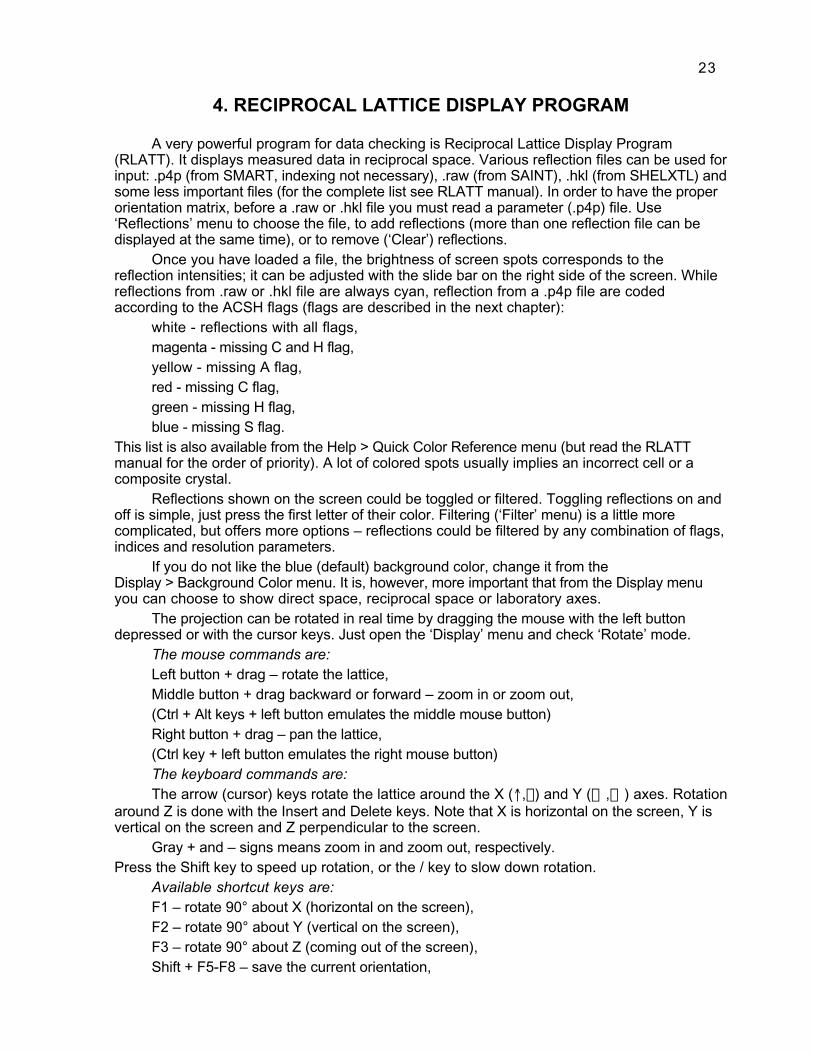
4. RECIPROCAL LATTICE DISPLAY PROGRAM

A very powerful program for data checking is Reciprocal Lattice Display Program(RLATT). It displays measured data in reciprocal space. Various reflection files can be used forinput: .p4p (from SMART, indexing not necessary), .raw (from SAINT), .hkl (from SHELXTL) andsome less important files (for the complete list see RLATT manual). In order to have the properorientation matrix, before a .raw or .hkl file you must read a parameter (.p4p) file. Use‘Reflections’ menu to choose the file, to add reflections (more than one reflection file can bedisplayed at the same time), or to remove (‘Clear’) reflections.

Once you have loaded a file, the brightness of screen spots corresponds to thereflection intensities; it can be adjusted with the slide bar on the right side of the screen. Whilereflections from .raw or .hkl file are always cyan, reflection from a .p4p file are codedaccording to the ACSH flags (flags are described in the next chapter):

white - reflections with all flags,magenta - missing C and H flag,yellow - missing A flag,red - missing C flag,green - missing H flag,blue - missing S flag.

This list is also available from the Help > Quick Color Reference menu (but read the RLATTmanual for the order of priority). A lot of colored spots usually implies an incorrect cell or acomposite crystal.

Reflections shown on the screen could be toggled or filtered. Toggling reflections on andoff is simple, just press the first letter of their color. Filtering (‘Filter’ menu) is a little morecomplicated, but offers more options – reflections could be filtered by any combination of flags,indices and resolution parameters.

If you do not like the blue (default) background color, change it from theDisplay > Background Color menu. It is, however, more important that from the Display menuyou can choose to show direct space, reciprocal space or laboratory axes.

The projection can be rotated in real time by dragging the mouse with the left buttondepressed or with the cursor keys. Just open the ‘Display’ menu and check ‘Rotate’ mode.

The mouse commands are:Left button + drag – rotate the lattice,Middle button + drag backward or forward – zoom in or zoom out,(Ctrl + Alt keys + left button emulates the middle mouse button)Right button + drag – pan the lattice,(Ctrl key + left button emulates the right mouse button)The keyboard commands are:The arrow (cursor) keys rotate the lattice around the X (↑,Ø) and Y (¨,Æ) axes. Rotation

around Z is done with the Insert and Delete keys. Note that X is horizontal on the screen, Y isvertical on the screen and Z perpendicular to the screen.

Gray + and – signs means zoom in and zoom out, respectively.Press the Shift key to speed up rotation, or the / key to slow down rotation.

Available shortcut keys are:F1 – rotate 90° about X (horizontal on the screen),F2 – rotate 90° about Y (vertical on the screen),F3 – rotate 90° about Z (coming out of the screen),Shift + F5-F8 – save the current orientation,

24

F5-F8 – restore a saved orientation.RLATT is extremely useful and you should run the program as often as necessary to

check the regularity of the reciprocal lattice and the values of the unit cell parameters. Ifeverything is OK, you should see regular rows parallel to the reciprocal axes. The phrase “asoften as necessary” means: each time you determine, or re-determine the unit cellparameters.

First of all, in case you see curved rows, or even duplicated spots, do not blame yourcrystal or your whiskey; most often it turns out to be an artifact of inaccurate detectorcorrection values (X, Y for the detector center too far off, or more often a wrong detectordistance), so check and try to correct this. If you sometimes see a nice circular orbit of spots inclose succession, it is an almost unmistakable sign of "hot spots" being included in your list ofreflections. If you are the type that likes to read telephone books or such, just go to yourreflection list (Edit > ReflArray in SMART) and look for repeating, almost identical Xs and Ys.Delete them (maybe back up your list first) and check again. Bet your orbits have disappeared.Another easier approach is to mark graphically the “ghost” spots in RLATT (see later how tochange flags and colors of the reflections), save the results in a file, edit it by throwing out themarked reflections and then use the edited file in further work.

It is not obligatory to have the true unit cell parameters in the .p4p file you use. It is stillpossible to verify the lattice regularity and measure distances between layers. Although themeasurements are not very accurate, the obtained values are good estimates for the nextround of unit cell determination.

How to measure distances between layers? Turn on Measurement mode(Display > Measure distance) first and zoom in the picture if necessary. Then drag the mousewith the left button depressed between the chosen start and end points. After you release theleft button RLATT will show the distance between two points in Å-1 (Fig. 4.1.a).

In this version of RLATT (3.0) there are two very good tools that help measurements. Usethem to increase the accuracy of your determination! If you press the Gray + key, you willsubdivide the current measurement with the new distance shown. It is, of course, possible torepeat this operation many times. In the opposite direction, the Gray – key reduces the numberof subdivisions. If you press the Page Up key, you will add extra divisions on each side of theexisting one (Fig. 4.1.b). They are of the same length as the previous divisions. (The PageDown key reduces the number of extra divisions.) For fine tuning you can use the cursor keys,which move the measurement tool, or Insert and Delete keys, which rotate the lattice around Z.

With RLATT it is also possible to see if the lattice is rectangular or not and to estimate theangles. The program is also useful for testing lattice centering. Try the following approach:

Turn the lattice until you notice a family of lattice planes with the largest spacing andorient it for an edge-on view. Measure the interplanar distance (the length of the correspondingcrystal lattice vector, call it a). Now turn the lattice parallel to the planes until another family ofplanes with a relatively large spacing appears. Try now to adjust the picture so that the newfamily of planes is oriented horizontal or vertical and you still see both families edge-on (not aneasy task!). Measure the second interplanar spacing/crystal lattice vector (call it b). If you havesome applicable angle-measuring device you can try to measure the angle between the twoplane families/vectors (gamma) on the screen. Now turn parallel to the second family of planeswith the help of the cursor keys (one click turns exactly one degree!) or with F1 or F2 (a 90-degrees rotation) until you see another good family of planes edge-on. Counting the clicks withthe cursor keys measures b*. The interplanar spacing of the third family gives the c-parameter,angle-measuring on the screen gives a. Positioning the third family of planes vertical orhorizontal and then turning by cursor keys until the first family of planes reappears edge-ongives a measure of g*. a*can now be measured by rotating the first family of planes until thesecond reappears again. If this was a triclinic case, let’s hope you remembered to keep youraxes oriented properly right-handed, and know how to use the elementary lattice mathematicsto calculate the final values!

25

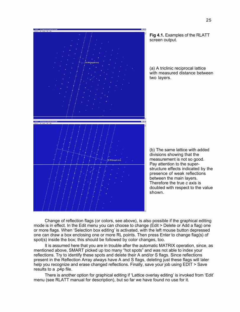
Fig 4.1. Examples of the RLATTscreen output.

(a) A triclinic reciprocal latticewith measured distance betweentwo layers.

(b) The same lattice with addeddivisions showing that themeasurement is not so good.Pay attention to the super-structure effects indicated by thepresence of weak reflectionsbetween the main layers.Therefore the true c axis isdoubled with respect to the valueshown.

Change of reflection flags (or colors, see above), is also possible if the graphical editingmode is in effect. In the Edit menu you can choose to change (Edit > Delete or Add a flag) oneor more flags. When ‘Selection box editing’ is activated, with the left mouse button depressedone can draw a box enclosing one or more RL points. Then press Enter to change flag(s) ofspot(s) inside the box; this should be followed by color changes, too.

It is assumed here that you are in trouble after the automatic MATRIX operation, since, asmentioned above, SMART picked up too many “hot spots” and was not able to index yourreflections. Try to identify these spots and delete their A and/or S flags. Since reflectionspresent in the Reflection Array always have A and S flags, deleting just these flags will laterhelp you recognize and erase changed reflections. Finally, save your job using EDIT > Saveresults to a .p4p file.

There is another option for graphical editing if ‘Lattice overlay editing’ is invoked from ‘Edit’menu (see RLATT manual for description), but so far we have found no use for it.

26

Some limitations of the program have to be emphasized. It is not possible to read out theangles or indices of individual lattice spots (although the latter can be guessed by counting in3D). Also, it would be very desirable to define shortcut keys that will display projections alongeither reciprocal or direct axes.

27

5. IF MATRIX OPERATION FAILS...

That happens more often than anybody wants and it is always very frustrating. Thequestion is: How to recognize the failure? The first case is very simple: if MATRIX was run inautomatic mode, any screen output after the procedure is missing. Apparently, SMART wastotally confused about your crystal and its reflections (and probably about you as well).However, sometimes the procedure offers really “funny” solutions with unit cell parameters of,say, 80, or even more Ångström. Finally, the results could be quite different from what youexpected (reconsider expectations).

It could be worth noting that some experienced crystallographers pay little attention to theMATRIX procedure, which serves them chiefly to verify that the crystal is suitable for datacollection – even if perhaps twinned. However, even they must pass through determination ofunit cell parameters and orientation matrix after data collection and before starting theintegration. Therefore, the procedures described here are universal, and they wait for youhere, there or in both places.

As a beginner, you have to analyze frames and reciprocal lattices (as described above),as well as reflections picked automatically or manually during the MATRIX operation. Theyare stored in a Reflection Array, which contains reflections used (or to be used) for unitcell determination. Running any of the following commands:

•fi EDIT > ReflArray, CRYSTAL > Redtn Cell > Edit, or Ctrl+E shortcut

will allow you to view and possibly edit the contents of the Reflection Array. An ACHSflag indicates the status of reflections.- A flag means that the reflection record includes goniometer setting angles and X, Ycoordinates of the reflection relative to the detector origin; this is always the case forreflections determined experimentally.- S flag indicates that the values of the X,Y spot positions of this reflection have beencorrected with a spatial correction; this condition is also always satisfied forexperimentally determined reflections.- C flag denotes centered reflections, that is, there was enough information to determinethe centroid inside the scan angle; the necessary condition is that the reflection is visibleon (or spanned by) more than one frame.- H flag means that the reflection has HKL indices; of course, this is possible only afterindexing.The other data in Reflection Array are: HKL indices (if determined), 2-theta, omega, phi,and chi angles, X and Y detector coordinates of the centroid, normalized intensity (I) andI/sigma ratio.It is possible to modify any entry, to change flags, to delete some, for example, veryweak or very strong reflections, to type in some already known data, or to add somereflections by an interactive means provided by CRYSTAL > Redtn Cell > Pick, which willbe described below.

!!! Be very careful, one of the SMART bugs flies around, watching and waiting for you to fallin its trap. After you finish editing the Reflection Array it is normal to click OK to accept itsnew contents. Everything will be OK. However, if you meanwhile get the idea (veryclever) to press Write in order to save data (as an ASCII name.txt file for example) ondisk just for reasons of insurance, possible future usage, or just for documentation, andif something in Array is accidentally marked (blue background, white letters), only themarked part of the Array will be written to disk. A really amusing extraterrestrialphenomenon! It is, indeed, so easy to lose all of your several-hours effort, especially ifdata in the current matrix#.p4p file were later “spontaneously” (as defined by Murphy’slaw) rewritten, reindexed, etc. The same is true for printing.If the problem is wrong or missing indexing, there are at least six ways to proceed.

28

First of all, you can try to use and index/reindex (perhaps with some modifications)reflections already present in the Reflection Array. Sometimes only a small push is required to“help” the program find the “proper” solution(s). Here the Reciprocal Lattice Display Programand procedures described in the previous chapter could be very helpful.

If there is a suspicion of a composite crystal (twin or another intergrowth) we stronglysuggest you try indexing by GEMINI as a second option.

The third and fourth options imply that you will collect (automatically or manually) a newset of (medium to strong) reflections and attempt to index them.

The remaining two cases are in fact obvious, but we wish to leave them for the end ofthe chapter. (Why discourage beginners immediately?)

If you have been following our suggestions, you have already checked the collectedreflections using RLATT and got an idea about their usability. If it all looks just like a mess, youcould probably try autoindexing as described under option no. 1 by changing some parametersblindly. Maybe the program sees better than you and you really get something (but need tocheck to see if it is reasonable anyway). If you fail a few times, we suggest you do not wasteyour time anymore; proceed to the next options.

If you have seen the light (a real lattice!) then you are probably in a hurry to try approachnumber 1 right away. Good luck, you impatient soul! Oh, you took your time and alreadymeasured some lattice parameters? For your bureaucratic type there would be no problem toenter the expected parameters and small tolerances in procedure no. 1 and check 'Assumeknown cell' (see later).

Maybe you have seen too much light (several lattices in a beautiful confusion). Skipimmediately to option no. 2. Again you could be without any quantitative data, or with quite adetailed premeasurement in RLATT, but it depends on how you do other things in your life andyou will be rewarded accordingly.

1.If you decide to use collected reflections, i.e. reflections already present in the ReflectionArray (perhaps with some above-mentioned editing), check the number of reflections inArray. Remember: a maximum of 999 reflections can be stored in Array, 25 is an absoluteminimum for indexing, and, in accordance with BRUKER recommendations, a number inthe range 50-100 is about optimal at this stage. All reflections should be centered, i.e.have a C flag! Delete all non-centered reflections and all reflections with I/sigma less than30, or even 50, if you have too many suspect reflections in the Array. An alternativeapproach is to identify “hot spots” using RLATT, as described above, and to remove themfrom the Array. After that you can go to

•fi CRYSTAL > Redtn Cell > Index or Ctrl+X

which is also called “Autoindexing”. This command uses reflections stored (by Thresholdor by manual picking) in the Reflection Array to determine indices, a rough crystalorientation matrix and a reduced primitive cell. The autoindexing procedure is based on analgorithm operating on difference vectors (which are classified in groups) derived fromthe input reflections. If the procedure with difference vectors fails, the program triesindexing on full vectors.If you really believe that you know the true unit cell parameters (maybe they weredetermined previously, e.g. with the program RLATT, or you think you know them bysome providence, or those from MATRIX were good and you are in trouble after datacollection), go to the ‘Autoindexing’ menu (Ctrl+X), input the expected values for celledges and angles, enter ‘Length tol’ 0.1, ‘Angle tol’ 0.1 and check the small box (Fig. 5.1)near the ‘Assume known cell’. How the latter option influences the behavior of theprogram it is very hard to guess, but anyway... only a few seconds will be enough toreach extreme happiness or total devastation.

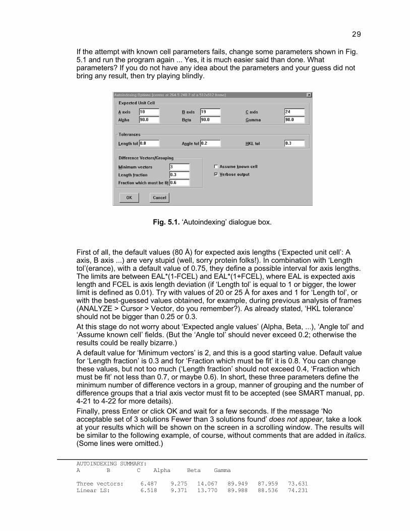
29

If the attempt with known cell parameters fails, change some parameters shown in Fig.5.1 and run the program again ... Yes, it is much easier said than done. Whatparameters? If you do not have any idea about the parameters and your guess did notbring any result, then try playing blindly.

Fig. 5.1. ‘Autoindexing’ dialogue box.

First of all, the default values (80 Å) for expected axis lengths (‘Expected unit cell’: Aaxis, B axis ...) are very stupid (well, sorry protein folks!). In combination with ‘Lengthtol’(erance), with a default value of 0.75, they define a possible interval for axis lengths.The limits are between EAL*(1-FCEL) and EAL*(1+FCEL), where EAL is expected axislength and FCEL is axis length deviation (if ‘Length tol’ is equal to 1 or bigger, the lowerlimit is defined as 0.01). Try with values of 20 or 25 Å for axes and 1 for ‘Length tol’, orwith the best-guessed values obtained, for example, during previous analysis of frames(ANALYZE > Cursor > Vector, do you remember?). As already stated, ‘HKL tolerance’should not be bigger than 0.25 or 0.3.At this stage do not worry about ‘Expected angle values’ (Alpha, Beta, ...), ‘Angle tol’ and‘Assume known cell’ fields. (But the ‘Angle tol’ should never exceed 0.2; otherwise theresults could be really bizarre.)A default value for ‘Minimum vectors’ is 2, and this is a good starting value. Default valuefor ‘Length fraction’ is 0.3 and for ‘Fraction which must be fit’ it is 0.8. You can changethese values, but not too much (‘Length fraction’ should not exceed 0.4, ‘Fraction whichmust be fit’ not less than 0.7, or maybe 0.6). In short, these three parameters define theminimum number of difference vectors in a group, manner of grouping and the number ofdifference groups that a trial axis vector must fit to be accepted (see SMART manual, pp.4-21 to 4-22 for more details).Finally, press Enter or click OK and wait for a few seconds. If the message ‘Noacceptable set of 3 solutions Fewer than 3 solutions found’ does not appear, take a lookat your results which will be shown on the screen in a scrolling window. The results willbe similar to the following example, of course, without comments that are added in italics.(Some lines were omitted.)

AUTOINDEXING SUMMARY:A B C Alpha Beta Gamma

Three vectors: 6.487 9.275 14.067 89.949 87.959 73.631Linear LS: 6.518 9.371 13.770 89.988 88.536 74.231

30

(Determined unit cell parameters before and after linear LS refinement.)......................................

Axis limits, max index: 0.100 20.000 0.100 20.000 0.100 20.000 5

(Axis a, b and c limits, followed by the maximum HKL index difference used to compute testsolution.)

# Length FOM H 1 H 2 H 3 Reflections fitAngles between solutions

(Just one unsuccessful attempt.)

Difference Vectors:

(Group, vector length, reciprocal space components of difference vectors, and number ofdifference vectors in groups.)

# Length X1 X2 X3 Freq 1 17.34149 0.01333 -0.05557 0.00603 3 2 13.77727 0.03155 -0.01323 -0.06229 2 3 13.57940 -0.01536 0.01654 0.06979 19... (truncated) 6 10.21316 0.09525 0.01918 -0.01106 2 7 9.00571 0.10372 0.03738 0.01322 12 8 8.55909 0.04534 0.01752 0.10567 2 9 8.36116 0.03602 0.04485 0.10392 4 10 7.51440 -0.11815 -0.02195 0.05717 10 11 7.49792 0.08936 0.05291 0.08367 13 12 7.48468 -0.08949 -0.05726 0.07984 2 13 7.36564 0.07051 -0.10349 -0.05061 2 14 6.81270 -0.02992 0.03044 0.14043 9 15 6.74176 -0.02958 0.02428 0.14277 5... (truncated) 51 4.27546 0.19292 0.09017 0.09673 7 52 4.26849 0.22215 0.05996 -0.04401 5

(Pay attention to difference vectors repeating many times!)

Retrying with next shortest vectorAxis limits, max index: 0.100 20.000 0.100 20.000 0.100 20.000 5

(Program was not able to find set of three solutions; it retries with next shortest vectors.)

# Length FOM H 1 H 2 H 3 Reflections fitAngles between solutionsRetrying with next shortest vectorAxis limits, max index: 0.100 20.000 0.100 20.000 0.100 20.000 5... (truncated)# Length FOM H 1 H 3 H 2 Reflections fitAngles between solutions

1 17.208 0.19 1 2 2 1111100111101001110111111110111101101101111011Indexing failed on difference vectorsFewer than 3 solutions foundRe-trying with first 100 full vectorsAxis limits, max index: 0.100 20.000 0.100 20.000 0.100 20.000 20

31

# Length FOM H 1 H 2 H 3 Reflections fitAngles between solutions

(Solution number, axis length, figure of merit - lower value is better, direction of axes, solutioncode: 1 for each vector group that fits and 0 for vector groups that do not fit. So, be happy if yousee a lot of 1s.)

1 9.275 0.17 1 0 0 11111111101111111101111111111111111111111000010000 1111111111110101110011111

2 6.487 0.09 0 0 1 11111111111111111111111111111111111111111011110111 1111111111111111101001111106.4

3 9.705 0.17 1 0 1 11111111101111111101111111111111111111111100010000 1111111111110101110101111 39.9 66.5... (truncated)

7 19.148 0.19 0 2 0 11111111101111111101110111111111001101110001110110 1110101110001011001101011125.5 59.9#102.7 47.3 125.5 114.9

(# denotes angles around 60 or 120°)

8 16.856 0.20 0 -2 1 11111111101111111101110111101011001101110000110110 1110101110001011011011010 56.6 100.6 66.2 119.7# 56.6 59.6#160.6

9 15.699 0.20 1 2 0 11111111111111111111111111111011001111110000011001 1111101110000001000001010 96.7 63.6 79.3 71.8 96.7 87.7 28.8 145.5

10 19.473 0.19 1 2 1 11111111111111111111111111111111011111111100010001 1110101110010101000101011100.9 46.2 73.6 60.7#100.9 86.8 29.1 136.6 17.4

11 14.067 0.20 1 2 -1 11111111111111111101111111101011101101110100011001 1111101110000011010001010 90.1* 88.0 88.7 88.9 90.1* 89.3* 41.7 146.6 24.4 41.7

(* denotes angles close to 90°)... (truncated)

23 19.053 0.18 1 0 3 11111111101111111101111111111111011111111101011100 1111111111000001001011010 78.5 27.8 38.6 72.2 78.5 58.1 76.7 85.4 66.6 52.0 87.9 62.1 46.1 82.0 27.8 65.3 12.8 57.6 110.0 38.6100.4 27.8

24 18.794 0.23 1 2 -3 11111111111101111101110111001011001101110100110110 0111101100000011001101000 78.8 131.6 105.0 118.7 78.8 92.3 77.7 119.8# 68.0 85.4 43.6 63.6 80.3 44.7 131.6 138.6 119.9#125.4 18.5 105.0 29.9 131.6 125.7

Predicted reduced primitive axes are:Soln# X Y Z Length 2 1.89857 -5.96602 1.69785 6.48696 1 7.52911 5.38987 0.53336 9.27484 11 -3.27490 3.28218 13.28097 14.06705

(X, Y, Z components of each vector and vector length.)

Reduced primitive cell is: 6.487 9.275 14.067 89.949 87.959 73.631

Least squares cell parameters: 6.518 9.371 13.770 89.988 88.536 74.231 809.06

32

Full vectors:

(Vector number, number of the closest vector, indices and reciprocal space vectorcomponents. H, K and L values should be close to integers!)

# NEAR H K L X1 X2 X3 1 33 2.97 0.99 0.09 0.15390 -0.41132 0.12468 2 22 3.98 1.97 1.75 0.16351 -0.59921 0.04324 3 33 1.99 0.98 2.06 0.10050 -0.31619 -0.06073 4 26 5.31 2.22 -1.65 0.20108 -0.72561 0.34113 5 7 3.93 2.65 1.45 0.08570 -0.61437 0.05200 6 30 1.98 0.06 -6.03 0.07347 -0.16333 0.51612 7 1 3.95 2.00 0.14 0.13477 -0.57320 0.15351 8 0 1.00 0.00 -1.02 0.07086 -0.11087 0.12017 9 4 5.26 2.82 -1.92 0.13067 -0.73831 0.34843 10 4 5.92 1.98 -4.82 0.23040 -0.74725 0.59538... (truncated) 74 57 -0.01 -4.06 -3.99 0.35796 0.21303 0.33867 75 34 -0.06 -2.75 3.18 0.32667 0.06574 -0.18256

Press Enter or click OK to exit the window. A message box with question ‘RE-INDEXREFLECTION ARRAY: ARE YOU SURE?’ will be displayed. Confirm ‘Yes’ button to writeHKL indices into the Reflection Array and to set the H flag of each indexed reflection.Then the program displays the next scrolling window with output very similar to theprevious one. That does not require additional explanation.If these attempts result in reasonable unit cell parameters, just follow the sequence listedin the CRYSTAL > Redtn Cell submenu of SMART window. It means that you have toexecute

•fi CRYSTAL > Redtn Cell > Bravais or Ctrl+B.

This operation determines possible Bravais lattices that will be ranked according to thesymmetry and goodness-of-fit (GOF). Normally, this command is invoked after the Indexand before the Least-squares operation, but all three commands store their results in thesame .p4p file. Therefore, unit cell parameters and their standard uncertainties arealways up-to-date and available to each other, and it is not always necessary to followthe listed order. E.g. if after indexing, the standard uncertainties of the lattice parametersare too high (and their accuracy too low) it sometimes causes an enormous list ofpossible Bravais lattices (many of them totally stupid). One can overcome this by firstperforming LS on the reduced cell parameters, lowering the standard uncertainties (e.g.by excluding reflections with too high RLV error) and then trying Bravais. The number ofsolutions will be drastically reduced.

Fig. 5.2. ‘Bravais Lattice’ dialogue box.

The program will suggest “the best” solution, meaning the highest symmetry lattice whosegoodness-of-fit is better than an input threshold. But you are free to choose any of the

33

listed solutions. Finally, Reflection Array will be automatically (re)indexed according to theselected unit cell.A Bravais lattice window is shown in Fig. 5.2. Unit cell parameters and their standarduncertainties (Current A axis, ..., Current ALPHA, ..., ESD of A, ...) are automatically filledin with the values supplied by the Index procedure. If you insist (but it is not necessary)you can set ‘Max sigmas, any’ and ‘Max sigmas, best’ fields. The first parameter is theGOF limit for the listed solution so that all solutions with GOF above this value will berejected. It is hard to imagine that a solution with GOF>10 could be correct. The secondparameter is the GOF limit for the “best solution” and solutions with GOF lower than thisvalue are potential candidates. The best solution is flagged with a ‘>>>‘ sign in the Bravaislattice output. Leave Lattice type as P, of course, after Indexing which determines areduced cell. However, the program also runs on centered lattices if e.g. you changedyour mind after accepting some centered solution.An example of a Bravais lattice output is listed below with added comments in italics. (Asusual, some lines were omitted.)

#Sigmas for acceptance of any soln, best soln: 20.0 6.0

Input lattice type: PInput cell and standard deviations: 6.518 9.371 13.770 89.988 88.536 74.231 809.06 0.077 0.125 0.253

Number of solutions = 96

# #Sig A B C Alpha Beta Gamma

(Number of solution, #Sig is GOF, “goodness-of-fit”, and unit cell parameters)RHOMBOHEDRAL(OBV); HEXAGONAL R SETTING 1 19.62 6.518 9.854 43.248 105.821 77.401 113.767 -1.00 0.00 0.00/ 1.00 -1.00 0.00/ -2.00 1.00 3.00/

(3x3 matrix that would transform the HKL indices from the input lattice to the latticecorresponding to the solution; the nine elements are in the order T11, T12, T13/ T21, T22, T23/T31, T32, T33/)

TRIGONAL P (NO C-AXIS SYMMETRY); HEXAGONAL P (C-AXIS SYMMETRY) 2 16.43 6.518 9.371 13.770 89.988 91.464 105.769 1.00 0.00 0.00/ 0.00 -1.00 0.00/ 0.00 0.00 -1.00/

3 18.45 6.518 9.854 13.770 89.044 91.464 113.767 -1.00 0.00 0.00/ 1.00 -1.00 0.00/ 0.00 0.00 1.00/

TETRAGONAL I 4 18.71 16.798 16.654 6.518 82.427 102.443 114.519 1.00 -1.00 -1.00/ 0.00 -1.00 1.00/ -1.00 0.00 0.00/

ORTHORHOMBIC F 5 11.07 6.518 18.092 28.137 89.459 101.926 94.516 1.00 0.00 0.00/ -1.00 2.00 0.00/ -1.00 0.00 2.00/... (truncated) 10 18.52 9.371 13.833 29.088 99.113 108.781 65.081 0.00 1.00 0.00/ -2.00 1.00 0.00/ 0.00 -1.00 2.00/

ORTHORHOMBIC I 11 18.47 6.518 16.798 16.654 65.481 82.427 77.557 1.00 0.00 0.00/ 1.00 -1.00 -1.00/ 0.00 1.00 -1.00/... (truncated) 14 19.88 6.518 17.065 16.657 64.879 79.980 75.326 -1.00 0.00 0.00/ -1.00 1.00 -1.00/ 0.00 -1.00 -1.00/

34

ORTHORHOMBIC C>>> 15 3.56 6.518 18.092 13.770 89.485 91.464 94.516 -1.00 0.00 0.00/ 1.00 -2.00 0.00/ 0.00 0.00 1.00/

(The “best solution” according to the program, since the highest symmetry is one of thecriteria. However, the angles are too far from 90° for an orthorhombic crystal.)

... (truncated) 16 16.09 9.854 12.786 13.770 89.245 90.956 68.913 1.00 -1.00 0.00/ -1.00 -1.00 0.00/ 0.00 0.00 -1.00/... (truncated)

ORTHORHOMBIC P 20 13.32 6.518 9.371 13.770 89.988 91.464 105.769 1.00 0.00 0.00/ 0.00 -1.00 0.00/ 0.00 0.00 -1.00/

MONOCLINIC C 21 3.35 6.518 18.092 13.770 90.515 91.464 85.484 1.00 0.00 0.00/ 1.00 -2.00 0.00/ 0.00 0.00 -1.00/... (truncated) 53 19.81 16.798 17.065 6.518 75.326 102.443 71.174 -1.00 1.00 1.00/ 1.00 -1.00 1.00/ 1.00 0.00 0.00/

MONOCLINIC I 54 10.32 16.798 6.518 16.654 97.573 114.519 77.557 1.00 -1.00 -1.00/ 1.00 0.00 0.00/ 0.00 -1.00 1.00/... (truncated) 65 19.81 16.657 17.065 6.518 75.326 100.020 115.121 0.00 1.00 1.00/ -1.00 1.00 -1.00/ -1.00 0.00 0.00/

MONOCLINIC P 66 1.25 6.518 13.770 9.371 89.988 105.769 91.464 -1.00 0.00 0.00/ 0.00 0.00 1.00/ 0.00 1.00 0.00/

(The proper solution for this case characterized by the next to lowest GOF value.)

67 13.27 6.518 9.371 13.770 89.988 91.464 105.769 1.00 0.00 0.00/ 0.00 -1.00 0.00/ 0.00 0.00 -1.00/... (truncated) 69 19.98 6.518 9.854 13.770 89.044 91.464 113.767 -1.00 0.00 0.00/ 1.00 -1.00 0.00/ 0.00 0.00 1.00/

TRICLINIC P 70 0.00 6.518 9.371 13.770 89.988 88.536 74.231 1.00 0.00 0.00/ 0.00 1.00 0.00/ 0.00 0.00 1.00/

(This solution, with the best GOF, is identical to the input and solution no. 66.)

71 3.30 6.518 9.854 13.770 89.044 88.536 66.233 -1.00 0.00 0.00/ -1.00 1.00 0.00/ 0.00 0.00 -1.00/... (truncated) 96 19.58 6.518 12.786 16.798 102.818 102.443 135.146 -1.00 0.00 0.00/ 1.00 1.00 0.00/ 1.00 -1.00 -1.00/

Sometimes the Bravais output may contain 500 solutions (upper limit) and it is hard to findthe best one suggested by the program. Do not worry, pressing Enter or clicking OK exitsthe Bravais output, and a new window, containing the number of the “best solution”appears. Just note the number, press Esc or click Cancel and you will be returned to theoutput window, allowing you to analyze the results in more detail. After you make theselection, press Enter again, type in YOUR OWN choice and continue. The reflections inthe Array will be (re)indexed accordingly.Note: Input zero if you for some reason want to discard. The other option is to input thenumber of the solution identical to the input (this is the one with #Sig=0.00, see the aboveexample).

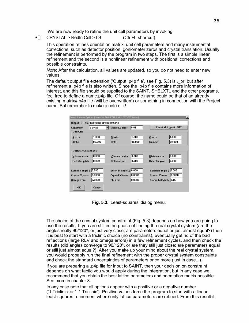
35

We are now ready to refine the unit cell parameters by invoking•fi CRYSTAL > Redtn Cell > LS.. (Ctrl+L shortcut).

This operation refines orientation matrix, unit cell parameters and many instrumentalcorrections, such as detector position, goniometer zeros and crystal translation. Usuallythe refinement is performed by the program in two steps. The first is a simple linearrefinement and the second is a nonlinear refinement with positional corrections andpossible constraints.Note: After the calculation, all values are updated, so you do not need to enter newvalues.The default output file extension (‘Output .p4p file’, see Fig. 5.3) is ._pr, but afterrefinement a .p4p file is also written. Since the .p4p file contains more information ofinterest, and this file should be supplied to the SAINT, SHELXTL and the other programs,feel free to define a name.p4p file. Of course, the name could be that of an alreadyexisting matrix#.p4p file (will be overwritten!) or something in connection with the Projectname. But remember to make a note of it!

Fig. 5.3. ‘Least-squares’ dialog menu.

The choice of the crystal system constraint (Fig. 5.3) depends on how you are going touse the results. If you are still in the phase of finding the real crystal system (are theangles really 90/120°, or just very close; are parameters equal or just almost equal?) thenit is best to start with a triclinic choice (no constraints), eventually get rid of the badreflections (large RLV and omega errors) in a few refinement cycles, and then check theresults (did angles converge to 90/120°, or are they still just close; are parameters equalor still just almost equal?). After you make up your mind about the real crystal system,you would probably run the final refinement with the proper crystal system constraintsand check the standard uncertainties of parameters once more (just in case...).If you are preparing a .p4p file for input to SAINT, then your decision on constraintdepends on what tactic you would apply during the integration, but in any case werecommend that you obtain the best lattice parameters and orientation matrix possible.See more in chapter 8.In any case note that all options appear with a positive or a negative number(‘1 Triclinic’ or ‘–1 Triclinic’). Positive values force the program to start with a linearleast-squares refinement where only lattice parameters are refined. From this result it

36

continues with a non-linear least-squares if the detector corrections or crystaltranslations are specified for refinement. Negative numbers mean that the linearleast-squares fitting is suppressed and the non-linear refinement will start from the latticeparameters as written in the dialogue boxes. It is advisable to use ‘1 Triclinic’ only the firsttime and then to continue with the ‘–1 Triclinic’ option or negative options for othersystems. (Unfortunately, the program always returns to the default positive value.) It issometimes necessary to try the positive option again if the suggested detectorcorrections get suspiciously high. Try setting them back to zero and starting a positivesystem constraint (especially if you are changing from triclinic to other systems).Note: If you select 0, the program performs only a linear refinement – not recommended.‘Max RLV error’ defines the maximum allowed difference between the observed andcalculated Reciprocal Lattice Vectors. If the difference is bigger than ‘Max RLV error’, thereflection is removed from the least-squares calculation, and its H flag is cleared. If somereflections are outside the tolerance, a box is displayed containing the message: ‘<N>REFLECTION(S) REMOVED FROM LS (OUTSIDE HKL TOL)’. Some times the number ofremoved reflections is too large; click Cancel and try with a looser tolerance. In the firststage of refinement ‘Max RLV error’ could be bigger, say up to 0.02, especially if least-squares removes too many reflections. Then it should be gradually decreased to 0.005,and preferably to a lower number (0.002 or 0.0015), as the final value.If you press ‘Constraint mask:’ on the right side, a new window opens, giving you anopportunity to define constraints for one or several variables. Usually, only crystaltranslations are constrained, as indicated in Fig. 5.3 by code 512.

Tip: Sometimes you can speed up refinement and avoid wandering into false minima byconstraining the system in the early stages. Similarly, if the least-squares procedureseems to go in the wrong direction, try to refine only part of the parameters at a time, forexample detector corrections only or cell dimensions only.If you are measuring crystal after crystal with the same detector distance, then it is agood idea to determine the 6 detector corrections by measurement of a standard crystalwhich should have accurately known lattice parameters and could be easily centered.You would then refine only detector corrections and use them subsequently for othercrystals as known parameters with code 768. (You would have to repeat the standardmeasurements regularly to assure that your corrections do not change by virtue of someblack magic.) We have ourselves rarely attempted standard measurement this way (onlyfor two cases of complex large crystals). Usually the lattice parameters come outsatisfactory, and detector corrections refine to reasonable values even with only limitedMATRIX data.

Tip: The correction for the crystal-to-detector distance, as calculated by SMART and SAINT,is strongly correlated with the scale of the cell dimensions. If very accurate celldimensions are important, leave the crystal-to-detector distance fixed during the least-squares refinement. Naturally, in this case the crystal-to-detector distance must be verycarefully calibrated with a test crystal.For a complete list of constraint codes see SMART manual pp. 4-32 to 4-33. An emptyfield means that all parameters are free to refine.

!!! Finally, remember to check or define ‘Frame halfwidth’ in the bottom right area of thedialogue box. The default value, 0.15, corresponds to the 0.3° frame width (as definedduring data acquisition (Matrix, MultiRun, etc.)After execution of the LS command a scrolling output window is displayed. The contentof the LS output is given below, together with some comments added in italics.

Orientation Matrix: -0.08826239 0.01603561 -0.10353260 0.12271879 -0.01568373 -0.03945471 -0.04739063 -0.07047869 -0.01477626

37

Lattice parameters & Standard deviations:6.5798 13.5205 9.3254 90.000 106.390 90.000 795.890.0026 0.0050 0.0034 0.017 0.014 0.015 0.81

(Very important tabular histograms follow! The first one shows differences between calculated andobserved H, K, L and scan angle values (in degrees). The second one shows differences fordetector X, Y positions (in pixels). In both histograms the numbers should be concentrated on theleft side. The best case is with all numbers in the first column.)Histograms: .00 .05 .10 .15 .20 .25 .30 .35 .40 .45 Inf H 81 0 0 0 0 0 0 0 0 0 K 80 1 0 0 0 0 0 0 0 0 L 81 0 0 0 0 0 0 0 0 0 Omega 31 16 15 6 3 4 3 1 1 1

0.00 0.25 0.50 0.75 1.00 1.25 1.50 1.75 2.00 2.25 InfX 38 25 14 4 0 0 0 0 0 0Y 28 25 9 11 5 3 0 0 0 0

H K L Omega X YAVG 0.001 -0.001 -0.002 0.000 0.000 0.000RMS 0.006 0.019 0.012 0.165 0.384 0.602

(Mean differences and their s.u.s. If AVG are bigger than RMS you may suspect misindexing ormisalignment of the system. A list of the 10 worst reflections follows.)Worst Agreements (worst RLV error):

# H K L dRLV dOMEGA10 -6.01 -4.95 1.98 0.0046 -0.20328 -3.01 -2.99 1.04 0.0044 0.43918 -3.01 -6.97 -0.02 0.0042 -0.33165 -1.00 -1.05 -5.00 0.0039 0.00420 -3.01 -4.98 -0.02 0.0038 -0.36417 -4.99 3.04 4.01 0.0038 0.04280 -1.00 -2.05 -4.99 0.0037 0.016136 2.01 -12.02 -1.03 0.0035 0.233135 2.01 -11.01 -2.03 0.0035 0.24161 -1.00 2.96 -6.00 0.0030 0.054

Detector corrections: X-Cen Y-Cen Dist Pitch Roll Yaw (additive) 0.284 -0.563 -0.051 0.048 0.486 0.031

(Detector corrections. Pay attention, if the first three values are greater than 1.0 for X- andY-Cen, and greater than 0.2 for Dist, perhaps the crystal was not as good as you thought, ormaybe the diffractometer requires adjustment. Contact administrator.)Eulerian angles: 126.620 92.855 -17.429Omega, Chi zeros: 0.9928 0.3876Crystal XYZ: 0.0000 0.0000 0.0000

(Pay attention to the ‘Omega, Chi zeros’ values that should be close to zero. Once again, theseparameters indicate quality of the crystal/data, or misalignment of the detector. Crystal translationswere not refined in this example.)

38

Nonlinear refinement: StartingRes FinalRes GOF #Cycles Code 2.21751E+01 1.74753E+01 15.67 2 0

(This line contains starting and ending residuals, goodness-of-fit, number of refinement cycles and acompletion code. GOF value higher than 10 indicate that the refinement is not so good. If the codeis not 0, rerun refinement with negative constrains. The list of all reflections in the Array follows.)

# Flags H K L Swing Omega Phi Chi X Y Inorm I/Sig1 ACHS -3 0 1 340.000 330.252 0.000 330.000 236.74 208.85 6954.5 106 +.00-.01+.00 -0.003 -0.18 -0.44

2 ACS -4 2 2 340.000 329.051 0.000 330.000 287.50 140.04 3994.7 80 +.02+.38-.01 1.214 3.71 10.90 …(truncated)5 ACS -4 1 3 340.000 337.153 0.000 330.000 287.44 140.04 2597.6 65 -.02-.31+.33 -3.877 -5.39 -4.31

6 ACHS -2 -6 0 340.000 334.444 0.000 330.000 221.89 402.64 3227.5 72 +.01-.01-.02 0.313 0.54 -0.77…(truncated)

If you at last have obtained good unit cell parameters (answer to the Frequently AskedQuestion - the meaning of “good” - will be presented in the next edition of this Guide),take a not too long break, skip all other options and jump to the chapter “Data collection (ordata acquisition) strategy.”Chances for success: almost better than none.

2.If you came here, it means that your crystal most probably is a complicated case, a twinor even an intergrowth of different phases. Congratulations! Simple cases are for lesstalented people. Real crystallographers like it hot! OK, it seems easy now to play cleverafter the magical program GEMINI appeared, but we are not such cowards, we really didsome intergrowths by optically cleaning reflection arrays in RLATT, and refining twolattices separately, then calculating their overlap ourselves and integrating. However,after GEMINI appeared, we would never try that again.GEMINI really works wonders. We still have not found the limit on the number of lattices itcan resolve. E.g. just from a matrix data collection on a microcline fragment (a triclinicmineral) with about 90 reflections total we easily determined both the twin law and theoriented intergrowth with quartz.So, try it. We are not going to give procedural advice here; the manual for GEMINI is veryinformative in itself. It even includes the full explanation of the indexing philosophy, tutorialand procedures for both SMART and GEMINI! We would wish the program were justslightly more flexible. It is designed exclusively to handle (non-merohedral) twins anddefragmented phases, but it can also resolve all kinds of multiphase intergrowths (and asmentioned, we use it for all kinds, but then have to handle some of the files our way).Chances for success: if you did not throw away such a crystal, nothing could stop youanyway.

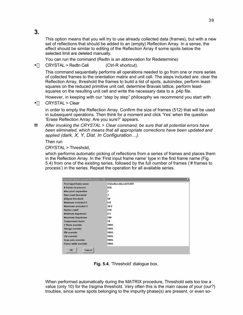
39

3.This option means that you will try to use already collected data (frames), but with a newset of reflections that should be added to an (empty) Reflection Array. In a sense, theeffect should be similar to editing of the Reflection Array if some spots below theselected limit are deleted manually.You can run the command (Redtn is an abbreviation for Redetermine)

•fi CRYSTAL > Redtn Cell (Ctrl-R shortcut).

This command sequentially performs all operations needed to go from one or more seriesof collected frames to the orientation matrix and unit cell. The steps included are: clear theReflection Array, threshold the frames to build a list of spots, autoindex, perform least-squares on the reduced primitive unit cell, determine Bravais lattice, perform least-squares on the resulting unit cell and write the necessary data to a .p4p file.However, in keeping with our “step by step” philosophy we recommend you start with

•fi CRYSTAL > Clear

in order to empty the Reflection Array. Confirm the size of frames (512) that will be usedin subsequent operations. Then think for a moment and click ‘Yes’ when the question‘Erase Reflection Array: Are you sure?’ appears.

!!! After invoking the CRYSTAL > Clear command, be sure that all potential errors havebeen eliminated, which means that all appropriate corrections have been updated andapplied (dark, X, Y, Dist. In Configuration…).Then runCRYSTAL > Threshold,which performs automatic picking of reflections from a series of frames and places themin the Reflection Array. In the ‘First input frame name’ type in the first frame name (Fig.5.4) from one of the existing series, followed by the full number of frames (‘# frames toprocess’) in the series. Repeat the operation for all available series.

Fig. 5.4. ‘Threshold’ dialogue box.

When performed automatically during the MATRIX procedure, Threshold sets too low avalue (only 10) for the I/sigma threshold. Very often this is the main cause of your (our?)troubles, since some spots belonging to the impurity phase(s) are present, or even so-

40

called “hot spots” (nonexistent spots) have been picked. You should play with theargument in the ‘I/Sigma threshold’ field, which is of special importance here. Try tochange this value in order to pick up over 30 reflections from a MATRIX series (about 100from all series).If you still do not obtain a satisfactory result, try adjusting some other parameters. ForMax pixel separation we still have not found what it can help, but Raw count thresholdcould be changed to an estimated background level (helps sometimes in case thereflections are rather weak). The value –1 lets the program guess on its own. You couldtry to navigate through some of the frames with ANALYSE > Cursor and mark the typicalcounts for the background, and the diffraction spots. Then use a value that is highenough to exclude all of the background and low enough to register the spots. Minimumand Maximum excluded X are used to exclude spots falling close to the vertical plane ofthe primary beam (in standard MATRIX runs it is close to the left edge of the frame: checkwith the shadow of the beam-stop). These spots belong to reciprocal lattice vectors thatpass very slowly through the Ewald sphere and are less accurately centered. Radiuscutoff and Minimum Angstroms could be used to exclude regions which are withoutreflections anyway; Maximum Angstroms cuts reflections with low diffraction angles(less accurate for lattice parameters). Wonder if you can get out something bymanipulating these values, but a smaller number in the 'Minimum Angstrom' field helps toget more reflections in the Array.It seems useful to decrease the temperature factor; its default value is highlyoverestimated, but the effect of decreasing the value is practically negligible. Leavedefault number 9999 for the last six parameters. It means that the corresponding data willbe extracted from the frames themselves.

Fig. 5.5. Threshold output. (‘Print’ means print on printer, ‘Write’ write data to disk.)

Threshold output written directly to the screen is not complicated (Fig. 5.5). Number ofobserved, centered, accepted, etc. reflections is listed first. The ‘Stored XY spot sizeand =‘ and ‘Stored Z FWHM spot size =’ (both are given in degrees) are transferredthrough the .p4p file (as MOSAIC parameter) to SAINT. They are maximum values andcan be a good estimate for the reflection size required by SAINT. Before them typicalvalues are given. Reflection statistics follows: Inorm means integrated intensitynormalized to 1°/minute, #Sig is I/sigma ratio, D represents resolution, Code C(hexadecimal system) means that the reflection is accepted, while reflections with theother codes are rejected.If the entire action results in a reasonable number of reflections, that is at least 25 ofthem, and preferably between 50 and 100 total in the Reflection Array, you shouldsequentially execute the commands listed above under option 1.

41

Chances for success: do not be dissatisfied.

4.This option means that you have decided to ignore that “blind, useless, stupid,#!�©?$+#_!��, ..., etc.” program. So, you will try to pick a new set of “morerepresentative reflections” manually by so-called “hand-picking.” Once again, the firststep is to erase the currently used reflections stored in the Reflection Array. Run

•fi CRYSTAL > Clear.

Now that you are sure you know what to do, confirm, once again, the size of frames(512) that will be used in subsequent operations and confirm ‘Yes’ when the question‘Erase Reflection Array: Are you sure?’ appears. Open a set of frames (Fig. 2.1) with

•fi FILE > Display (Ctrl+D),

choose the desired frame (usually the first in a series). Now, track a reflection fromframe to frame (remember: Ctrl+_ or Ctrl+_) until you find the frame on which it appearsthe strongest. Then execute

•fi CRYSTAL > Pick,

which provides an interactive means for adding reflections to the Reflection Array. Thiscommand is very similar to the previously described ANALYZE > Graph > Rocking andANALYZE > Cursor > Box ones (refresh your memory!), except that the reflection dataare now written into Array. As already stated, you should be very careful when definingthe correct box size (‘Width’, ‘Height’, Fig. 5.6). For this you can use a dialog box, screenediting, or both options successively.

Fig. 5.6. ‘Pick’ dialogue box.

!!! Check that the value of zero is specified in the ‘Reflection #’ field. This means that anynew reflection will be placed in the first available empty line of the Reflection Array. Incase you specify a number above 0, the reflection is written in the correspondingposition in the list, overwriting what previously was there. It is enough to have thenumber 3 in the ‘Frame halfwidth’ field, but if you are in the middle of a series put in abigger number (5, for example) here. Reflections will be better centered.

!!! Disregard the “flashes” which appear on one frame and occupy only a few pixels. Theseare most probably just “hot spots.”

!!! Picked reflections are automatically stored into Reflection Array after a left mousebutton click. Unfortunately, you will not be able to check the reflection before its profile isdisplayed on the screen. In case of a bad (not properly centered, split, very broad, tooweak, etc.) reflection, use EDIT > ReflArray (or Ctrl+E shortcut) immediately and deletethe reflection from the list.

42

Move to the next frame (Ctrl+Æ) and (later) to the next series of frames (Ctrl+D, asdescribed above) and repeat CRYSTAL > Redtn Cell > Pick command until you havesufficient (100 should be enough) data. It is important to have reflections from differentparts of reciprocal space! Use all available series of frames! Go to CRYSTAL > Indexand continue the work as described in option no. 1.Chances for success: not so bad, but could be better.

5.If all previous attempts fail, and you decide to use the same crystal (single, or not sosingle, that’s the question now!), then run

•fi ACQUIRE > Matrix

again. This time you have to be very, very cautious during the choice of parameters in thecorresponding dialogue box (see above). Usually, you have to increase the number offrames to be collected, as well as the exposure time. Very often this has to beaccompanied by a decrease in ‘Frame width’. Also, you should consider detector tocrystal distance (usually set between 4 and 6 cm). In case of high-symmetry crystalsand short crystal-lattice periods a shorter distance (e.g. 3 cm) allows more data to becollected and increases the chance for success. If reflections are overlapped (at leastone cell parameter big) try with a longer distance. This time set in advance ‘Indexing HKLTolerance’ to 0.2-0.25 and ‘LS RLV Tolerance’ to 0.02.Chances for success: if the crystal is indeed of good quality, maybe even slightly betterthan you expect.

6.Find a better (?) crystal, define a New Project, or edit the existing one, and start from thebeginning. Follow procedures described in chapters CRYSTAL MOUNTING andORIENTATION MATRIX. Good luck!Chances for success: depends on the quality of your crystals and weather forecast, butif you really are a gambler why not try for the jackpot?

If you read this chapter carefully, it was impossible to miss the observation that the sumof probabilities for success is very close to 100 %, perhaps a few percent above. Believe it ornot!

Finally, it is of course possible to take some combination of the above-describedapproaches. Almost everything depends on your imagination! It is also very helpful if you knowwhat you are looking for. But, if data do not support your prediction, do not reject the data forthat reason. Revise your theory or leave this science and turn to religion!

Tip: In our experience, when you use SMART and RLATT together, you should first of allclean up the Reflection Array from bad reflections and "hot spots" and then try to re-index reflections. If this does not help, go to option no. 3.

43

6. DATA COLLECTION (or DATA ACQUISITION) STRATEGY

General description and four-circle diffractometer

SMART allows data collection as a single run, or as a series of runs named “multipleruns”.

The single run is usually preferred for specimens mounted in capillaries. It is invoked bypressing

•fi ACQUIRE > Single Run command,

and it will not be described in detail.

The multiple runs are: Quadrant, Hemisphere and MultiRun. There is no importantdifference between the corresponding lists, since Quadrant and Hemisphere can beconsidered as subsets of the MultiRun procedure. While Quadrant is suitable forcollecting a wide-scan data set for an initial structural analysis (and will be only rarely, ormore likely, never used), the Hemisphere means that at least half of the Ewald sphere willbe collected. The MultiRun might be set up for a complete Ewald sphere collection with ahigh redundancy. We strongly suggest that you consider collecting a full sphere in anycase. It still would take just a fraction of the time required for a routine data collection on adiffractometer with a point detector. At the same time the accuracy of your latticeparameters and intensities of the merged symmetry equivalent reflections wouldsignificantly improve over the quadrant/hemisphere measurements and be at leastcomparable to those of the best old diffractometers.Commands that allow you to check, create or edit a run list are:

•fi AQIURE > EditQuad, AQIURE > EditHemi and AQIURE > EditMulti.

The utility programs ASTRO and COSMO, described in the next chapter, could be used tooptimize the run list for different crystal to detector distances, wavelengths, hardwareconfigurations, and crystal symmetry and unit cell parameters. See below and the nextchapter for more detailed discussion of this subject. Several examples and default valuesprovided and described in the SMART manual, pp. 2-1 to 2-5, could be helpful.Each of the commands mentioned has its own separate run list, but they are very similarand always contain the following data (Fig. 6.1):Run# Frame# 2-Theta Omega Phi Chi Axis Width #Frames Time‘Run#’ is simply the run number that will be used for the series. ‘Frame#’ is the startingframe number in the series. ‘2-Theta’ and ‘Chi’ are goniometer angles for the frame seriesscans. ‘Omega’ and ‘Phi’ are goniometer angles at the start of the frame series scans. Inthe next, ‘Axis’ field, 2 for omega, or 3 for phi scan should be specified (depending onwhich of them should be changed during the run). ‘Width’ is scan width (in degrees) ofeach frame to be acquired. ‘#Frames’ is number of frames collected in the series, while‘Time’ is exposure (accumulation) time for each frame in seconds.As seen in Fig. 6.1, the first two series represent phi scans. Each series comprises 186°,i.e. together they make more than a 360° scan around the phi axis. This is a commonsituation and nearly all MultiRuns involve such combinations of scans. It is of coursepossible to collect full 360° data in a single series. The only disadvantage is that afternumber 999, frames will get a combination of letters and numbers in the extension - a littlemore difficult to follow.

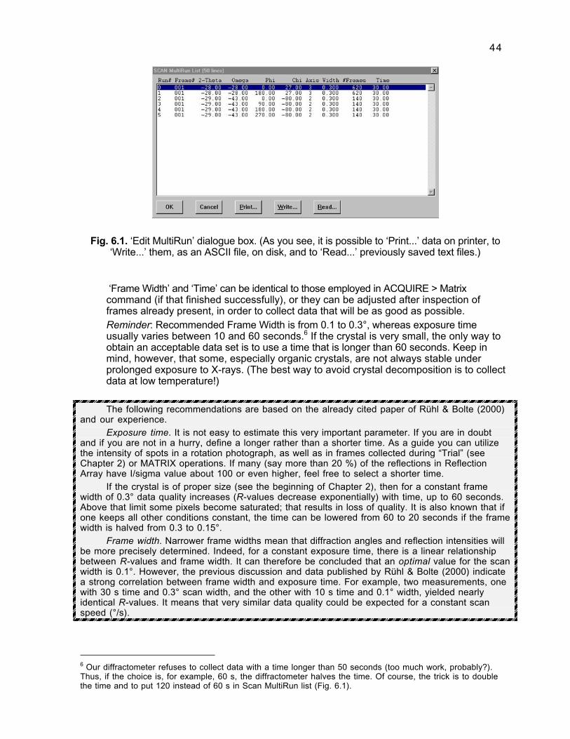
44

Fig. 6.1. ‘Edit MultiRun’ dialogue box. (As you see, it is possible to ‘Print...’ data on printer, to‘Write...’ them, as an ASCII file, on disk, and to ‘Read...’ previously saved text files.)

‘Frame Width’ and ‘Time’ can be identical to those employed in ACQUIRE > Matrixcommand (if that finished successfully), or they can be adjusted after inspection offrames already present, in order to collect data that will be as good as possible.Reminder: Recommended Frame Width is from 0.1 to 0.3°, whereas exposure timeusually varies between 10 and 60 seconds.6 If the crystal is very small, the only way toobtain an acceptable data set is to use a time that is longer than 60 seconds. Keep inmind, however, that some, especially organic crystals, are not always stable underprolonged exposure to X-rays. (The best way to avoid crystal decomposition is to collectdata at low temperature!)

The following recommendations are based on the already cited paper of Rühl & Bolte (2000)and our experience.

Exposure time. It is not easy to estimate this very important parameter. If you are in doubtand if you are not in a hurry, define a longer rather than a shorter time. As a guide you can utilizethe intensity of spots in a rotation photograph, as well as in frames collected during “Trial” (seeChapter 2) or MATRIX operations. If many (say more than 20 %) of the reflections in ReflectionArray have I/sigma value about 100 or even higher, feel free to select a shorter time.

If the crystal is of proper size (see the beginning of Chapter 2), then for a constant framewidth of 0.3° data quality increases (R-values decrease exponentially) with time, up to 60 seconds.Above that limit some pixels become saturated; that results in loss of quality. It is also known that ifone keeps all other conditions constant, the time can be lowered from 60 to 20 seconds if the framewidth is halved from 0.3 to 0.15°.

Frame width. Narrower frame widths mean that diffraction angles and reflection intensities willbe more precisely determined. Indeed, for a constant exposure time, there is a linear relationshipbetween R-values and frame width. It can therefore be concluded that an optimal value for the scanwidth is 0.1°. However, the previous discussion and data published by Rühl & Bolte (2000) indicatea strong correlation between frame width and exposure time. For example, two measurements, onewith 30 s time and 0.3° scan width, and the other with 10 s time and 0.1° width, yielded nearlyidentical R-values. It means that very similar data quality could be expected for a constant scanspeed (°/s).

6 Our diffractometer refuses to collect data with a time longer than 50 seconds (too much work, probably?).Thus, if the choice is, for example, 60 s, the diffractometer halves the time. Of course, the trick is to doublethe time and to put 120 instead of 60 s in Scan MultiRun list (Fig. 6.1).

45

It can be concluded that a frame width of 0.1° is probably too small, as well as that thedefault frame width of 0.3° is probably a little too big. In normal, everyday experiments it is advisableto use 0.20 to 0.25° frame widths. If the selected frame width is 0.2° and the crystal is of optimalthickness, it would be possible to collect the data using 30±20 s time in most cases.

Crystal-to-detector distance. Because the data quality depends on the reflection intensities, itis reasonable to expect that shorter distances are preferable. In a series of experiments with crystal-to-detector distances varied between 3.0 and 9.0 cm Rühl & Bolte (2000) obtained the best resultsfor 6.0 cm. However the differences in R-values for 3.0, 4.5 and 6.0 cm were practically negligible(although at shorter distances one can expect spot shape distortion). On the other hand, a longerdistance improves the signal-to-background ratio and a shorter distance allows collecting morereflections in the same time. Accordingly, under normal circumstances distances between 4.0 and6.0 cm could be recommended. “Normal circumstances” means that the biggest unit cell parameteris not above approximately 25 Å for 4.0 cm, and above 40 Å for 6.0 cm.

In case of a big unit cell, the detector has to be moved away in order to avoid reflectionoverlap. Several slightly different equations have been proposed for that purpose. In the simplestapproach the crystal-to-detector distance (for a primitive lattice) can be calculated from the relation

distance (in mm) = 1.5 ¥ a (in Å)where a is the longest unit cell axis. For high-quality crystals with sharp reflections the distancecould be even shorter. For low-quality crystals with broad reflections the spot size for integrationmust be very carefully determined or the detector distance must be longer.

Phi or omega scan? In few words, the choice of phi or omega scan is of no greatsignificance. Although phi scans result in slightly lower R-values (in particular wR2), there is no bigdifference in the quality of data collected by one or the other scan. (Actually, a combination of phiand omega scans is very common in the case of four-circle diffractometer, while phi scan is almostnever used on three-circle diffractometers.)

Redundancy. On a conventional point detector the intensities of reflections and their angularadjustments are very precise. This is not the case with an area detector, and individually collecteddata could be of lower quality. Nevertheless, area detectors have many advantages:

- data collection is very fast,- a complete diffraction picture is recorded and a wrong initial assignment of unit cell

parameters could be (easily?) corrected (impossible with a conventional detector),- it is common practice to collect symmetry-equivalent reflections up to the whole diffraction

sphere.By collecting many symmetry-equivalent or identical (at different 2-theta angles) reflections,

which means great redundancy, the quality of the final data set (containing averaged reflections)will approach that from a point detector. Therefore, it is really worth spending time measuringequivalent reflections. Rühl & Bolte (2000) showed that wR2 significantly decreased up to aredundancy of about 6 and after that slowly increased. At the same time, R1 and R(sigma)decreased in the whole interval and did not reach a minimum, even for a redundancy as high as 25.

Of course, the extent of possible redundancy depends on crystal symmetry and unit cellvolume; it correlates with crystal-to-detector distance too. In the case of triclinic and monocliniccrystals data collection strategy must be very carefully planned in order to reach full coverage andmaximum redundancy.

In conclusion, it is advisable to achieve as much redundancy as crystal symmetry and timeavailable permit. Therefore, in practice you will always choose runs that cover at least a hemisphereof reciprocal space.

According to a suggestion of Dr. Ibers (private communication), instead of making a singlemeasurement of one reflection in time t, it is better to make N measurements, each in time t/N. (Ofcourse, the t/N -value must be some reasonable number of seconds.) This is very probably true forlarge and well-diffracting crystals, but they require a face-indexed absorption correction.

46

!!! Before you run any type of scan, ensure that it agrees with collision limits (defined inGONIOM > Limits) for your particular system. If you are trying a data collection strategythat has never been used before on the instrument, a check of scan angle limits with thehelp of the manual box is COMPULSORY!

!!! Do not forget to acquire a new dark frame immediately before the start of data collection.In order to obtain the proper background correction, a dark frame MUST BE MEASUREDusing the same time as the time for frame scans. Give the dark frame a proper name,following the convention described in chapter “Directory (folder), names and extensionsof Bruker files”.

•fi If this has not already been done, run

GONIOM > Home Axis,which checks the calibrated position control of the goniometer circles, so that thereported position is exactly correct.

Fig. 6.2. ‘MultiRun’ dialogue box.

Now you are ready to collect data, that is, to run one of the commands:•fi ACQUIRE > Quadrant,

•fi ACQUIRE > Hemisphere, or

•fi ACQUIRE > MultiRun.

Just take a look at the MultiRun dialogue box (Fig. 6.2), change, if necessary, ‘Job name’and press Enter, or click OK.

A MultiRun scan interrupted for any reason can be continued using theACQUIRE > Resume command.

Beside the commands summarized above, under the ACQUIRE menu you can collectorientation matrix (ACQUIRE > Matrix) and rotation photograph (ACQUIRE > Rotation). Thesetwo options are described above. A single “still frame” at a fixed goniometer position(ACQUIRE > Still) and an omega-rotation picture with the crystal rotated around the a, b, or caxis (ACQUIRE > Axis command) could also be acquired. See SMART Manual pp. 2-14 to 2-17for more detail.

47

Three-circle platform diffractometer

After a reasonable cell has been determined, you can start data collection. The three-circle geometry results in some changes to the measurement strategy. Beside the fixed chiangle, the main difference is in scan axis, which is (almost always) omega7 in the case of athree-circle diffractometer.

Fig. 6.3. The Edit Hemi window. Enter all the required run parameters here. Values can beconveniently taken from the run table given in Appendix.

The main set-up window (Fig. 6.3) is reached by•fi Acquire > Edit Hemi.

This is where you enter the data that determine the data collection run.The table in the appendix lists different parameters for different total measurement timesand a crystal-to-detector distance of about 4 cm. To use, copy one of the run set-upsinto the Edit Hemi window.Note: The 3°-frame width will usually give a structure solution, but the R index tends tobe higher than most people like. Other frame widths typically have worked well, includingthe one at 1°.The estimated data collection times are for the frame times given. Different frame timescan be selected; for example, 10 s for a 0.3° frame width is often a good choice; ofcourse, it depends on how well the crystal diffracts.

!!! Be sure the dark-current time corresponds to the frame time entered.After you have finished setting up the run, do

•fi ACQUIRE > Hemisphere.

Enter jobname and click OK. Let the diffractometer collect the data set. Furtherprocessing is described below in chapter Data reduction strategy.

7 It is possible to perform a phi scan on the three-circle diffractometer and there are cases where it may givebetter data (e.g. for a strongly absorbing needle-like crystal mounted along phi). However, generally there aremany disadvantages of phi against omega scan.

48

7. STRATEGY PLANNING TOOLS

The simplest way to prepare (?) a data collection strategy is to skip this annoying step.Of course, you must have some parameters in the above-described ‘MultiRun’ or ‘HemisphereRun’ dialogue box, but it is always possible to leave the values that have been, who knowswhen and why, written in the smart.ini file as defaults. The results will most probably bequestionable. Also, you can utilize (blindly) some old scan data from a previous data collectionfor a crystal with similar symmetry and unit cell parameters. Not a bad concept, but still not fullyrecommendable, since orientation matrices would not be the same.

However, it is a good idea to prepare a library of ‘MultiRun’ scans that should be codedaccording to detector distance and frame widths. That can make your life much easier,especially if possible scans are related to the crystal data (may be in your notebook). Data fromthe library could be used later, at least as a starting point for consideration in ASTRO orCOSMO. So, after briefly playing with suitable ASTRO/COSMO commands, it should be possibleto find an adequate strategy for data collection. (In our laboratory in Copenhagen such a libraryis located in directory c:\frames and will be described later.) Even if you decide to use some oldscans, always check completeness and redundancy of data by ASTRO or COSMO.

ASTRO

ASTRO is an interactive and useful graphics program for determination of an efficientdata collection strategy during MultiRun scan. ASTRO is excellent for educational purposes,too. The program uses the well-known Ewald sphere concept in order to visualize andcalculate the volume of data in the scan. The area detector is presented as a projection on thesurface of the Ewald sphere. It is possible to simulate goniometer movements, as well as todisplay and record the segment of the reflecting sphere that passes through the detectorprojection. It is also possible to calculate the completeness and redundancy of data,corresponding to the currently displayed or input scans and, of course, in accordance with thechosen Laue group. Indeed, many possibilities exist. However, only elementary operations willbe described here.

When ASTRO is started you will see a graphical screen containing much visual andtextual information in different colors. Sometimes it is not easy to orient oneself in all those dataand the table above could be useful. In addition, on the right side of the screen, in the so-called“Status area”, you will see the current goniometer angles, current drive speeds, crystal Lauegroup, name of the current .p4p file, detector to crystal distance, X-ray wavelength, desiredresolution and a visibility state indicator for objects in the diagram.

With the help of listed shortcuts, which act as toggle on/off buttons (or, with the sameeffect, by commands listed in the EDIT menu), you can choose which objects will be visible. Atthe same time, the last item at the right bottom side of the screen (Fig. 7.1) indicates object‘Masks’, i.e. status of its visibility.

Laboratory axes are direct beam, or X axis (BEAM), the other horizontal, or Y axis (Y)and the vertical Z axis that coincides with omega and 2-theta and is oriented upwards (notshown). They form a right-handed coordinate system.

Goniometer axes are omega, chi and phi.The Ewald sphere is a sphere of radius 1 (in units 1/l) centered at the (–1, 0, 0) point.

49

OBJECT DEFAULT COLOR * SHORTCUT **

Laboratory axes (BEAM, Y) blue LGoniometer axes (Omega, Chi, Phi) pink GDetector projection on Ewald sphere red DEwald sphere blue EReciprocal axes (H, K, L) yellow RToroids green TReduced HKL data cyan HUnique volume white USymmetry equivalents purple M

* It is possible to change default colors using the EDIT > Colors command.** Available ASTRO menu commands and corresponding shortcuts are listed in the ASTRO

Manual, pp. A-1 to A-3.

During the scan the lattice is rotated about the goniometer center, and the volume of thereciprocal lattice that passes through the detector projection on the Ewald sphere will berecorded. The detector projection is like a cap on the Ewald sphere. Reciprocal axes are A*, B*and C* crystallographic axes (directions coincide with H, K, L).

a) b)

Fig. 7.1. ASTRO screen without (a) and with toroids (b) shown.

Toroids (green) can be described as possible scans. The aim of the data collectionstrategy is to fill an asymmetric unit (or unique volume) of the reciprocal lattice with them.

The unique volume represents an asymmetric unit of data chosen in accordance with theLaue group specified in the Symmetry menu.

‘Symmetry equivs’ is active if the Symmetry > Map_symmetry option is enabled. With thisoption portions of the scan toroids outside the unique volume are symmetry-mapped into it.

The viewing direction can be easily chosen using VIEWPOINT menu commands (orcorresponding shortcuts, see the ASTRO manual for a detailed explanation). The viewapproximately down the omega (Z+) axis is a good viewpoint to be used when performingscans interactively. Use the F3 shortcut to specify this view. The views down the crystal axes(F9, F10 and F11 shortcuts) are especially useful for examining completeness of coverageafter the scans have been defined.

50

The left and right arrow keys can be used for rotating the viewpoint around the screen Yaxis (vertical). With the up and down arrow keys it is possible to adjust the zoom (up = zoom in;down = zoom out).

The best way to familiarize oneself with the ASTRO graphical window is to turn differentitems on and off, using shortcuts from the previous table. You can start with an empty windowand then make any combination of items. Finally, select the red-green stereo view with theEDIT > Stereo Mode command (shortcut S), put on red-green glasses and play with the cursorkeys in order to obtain a good viewing angle. Also try different views using commands from theVIEWPOINT menu.

The data required to run ASTRO are crystal orientation matrix, which should be read fromthe corresponding .p4p file with FILE > ReadMatrix. (Orientation matrix can also be enteredmanually using EDIT > Configuration command.) In addition, you have to check and possiblyadjust some configuration parameters: ‘X-ray wavelength’, ‘Crystal to detector distance’,desired ‘Resolution’ (this directly influences the coverage calculation), ‘Frame Width’ and‘Frame Time’. Finally, it is important to know the Laue group (class) of the crystal, which isdetermined during the Bravais lattice command in SMART. If you are not quite sure about theLaue class, use the lowest symmetry group for the corresponding crystal system.

Of course, it is also very important to consider collision limits at the specified crystal todetector distance. Although it is possible to use slightly broader goniometer collision limits, forour diffractometer they are defined (in degrees) as:

Positive 2-theta limit 110Negative 2-theta limit –110Positive omega limit 45Negative omega limit –45Positive omega minus 2-theta limit 40Negative omega minus 2-theta limit –20Both phi and chi limits are set to 0, meaning free rotation around these axes. (You can

see the limits using EDIT > Limits or GONIOM > Limits commands in SMART or usingSTRATEGY > Limits command from ASTRO.) Do not change the limits defined in SMART, andput the same values, if necessary, into ASTRO! They should be kept in mind when you areplanning a data collection strategy.

Now you are ready to continue with ASTRO hunting. Select different resolution limits inEDIT > Configuration and note how the unique volume increases. Input shorter crystal todetector distance and you will se how the detector projection increases, too.

Required resolution (dmin) is a very important parameter here. It represents a lower limit ind-values for observed reflections and is related to the upper limit of the theta angle in the Braggequation (l = 2dminsinqmax). The best resolution that usually can be attained with Mo radiation isabout 0.6 Å (qmax ª 35°; 2qmax ª 70°). For an explanation, we can imagine that the unit cell is cutinto many slices, each of width dmin. Thinner slices allow insight into finer structure details.

For most structures such high resolution is unnecessary (0.8 Å would be enough)unless, of course, you are doing charge-density studies. A choice of desired resolution alsodepends on the scattering power of the investigated crystal. If you take a look at framescollected during MATRIX operation, you will see that in some cases the diffraction spots areconcentrated close to the shadow of the beam stop, while in some other cases spots arevisible in the entire frame. (Use the crosshair cursor to determine 2q-angles and resolution ofthe most distant reflections.) If the crystal does not diffract at high angles, it is useless torequire high resolution. Keep in mind, also, that a qmax of 25° for Mo radiation or 67° for Curadiation is the minimum requirement for publishing small-molecule structures in Acta Cryst., butuse higher values if the crystal diffracts sufficiently.

As a first step you can try to cover the asymmetric unit (unique volume) by passing ittrough the cap of the detector projection. Use the F3 shortcut to select a view down the Z+

51

axis. With STRATEGY > Drive or STRATEGY > Scan (Custom), swing the detector projection toa position where one side just covers the X-ray beam axis. Then drive the other goniometerangles to put the asymmetric unit in an orientation where rotation about Z will cover as large apart of its volume as possible. Sometimes it could be useful to select another possibleasymmetric unit. This can be done with SYMMETRY > Increment (Ctrl+Shift+I shortcut). Tryrotating about Z with phi (at chi = 0) until the asymmetric unit is inside the Ewald sphere with itsleading edge just behind the detector projection. [By making rotations of phi and omega (theusual rotation angles) it will be possible to find a good starting position. Keep in mind that phi isleft-handed, while omega is right-handed.] In this position a left-handed rotation about Z wouldmove the asymmetric unit through the sphere.

Next perform a scan. Select Omega Scan from the STRATEGY menu. Drive the scanangle (omega or phi) with the STRATEGY > Omega- (Alt+Num2 shortcut) or STRATEGY > Phi+(Num3 shortcut). Move the scan axis until the entire asymmetric unit has just passed throughthe detector projection. Then select STRATEGY > End Scan and the scan will be stored in therun list.

You can check and edit the run list using STRATEGY > Editruns.The possibilities of ASTRO are enormous. If, for example, you add a new run into the run

list and press Enter, a new group of toroids automatically appears on the screen. Therefore itis not really necessary to run the simulated goniometer. With a little experience you canguess a good scan, add it into the run list and see the results.

If you are going to collect a full sphere of data (or as much as possible) the best way isto have a full phi scan and supplement it with some omega scans that result in full coverage(the calculation of coverage is described below). So, you would start by entering the full phiscan in Editruns. By adjusting chi for this scan so that the calculated coverage is largest(typical values around ±30° ) one can find a good starting run and continue with several omegascans that give the maximum coverage and desired redundancy.

As already stated above, some old scan data could be a good starting point for thestrategy determination. They can be read (and written) from the ‘Edit MultiRun’ dialog box inSmart (Fig. 6.1) and the corresponding ‘Editruns’ box in ASTRO. Our library of scans (do youremember, in c:\frames directory?) is organized as text ASCII files (extension .txt). The namesare coded as

rdd_fwl.txt,that means:run + detector distance (in mm) + _ (just a separator) + frame width (in hundredths of adegree) + letter (necessary to differentiate scans with the same combination of distance andwidth).

For example r40_25b.txt represents a MultiRun scan for detector distance 40 mm, framewidth 0.25°, option b.

52

Reminder. Columns are:Run# Frame# 2-Theta Omega Phi Chi Axis Width #Frames Time

The above-mentioned r40_25b.txt file contains the following lines: 8

0 001 -38.00 -38.00 .00 27.00 3 .250 720 10.00

1 001 -38.00 -38.00 180.00 27.00 3 .250 720 10.00

2 001 -38.00 -50.00 .00 220.00 2 .250 200 10.00

3 001 -38.00 -50.00 90.00 220.00 2 .250 200 10.00

4 001 -38.00 -50.00 180.00 220.00 2 .250 200 10.00

5 001 -38.00 -50.00 270.00 220.00 2 .250 200 10.00

and represents a suitable starting point for strategy definition at 4.0 cm detector distance. Atemplate file rEdit.txt is also prepared in order to avoid extensive typing each time you try todefine a new strategy.

From some reason that only the Bruker guys can understand (remember the saying: “Theleft hand doesn’t know what the right hand is doing”) MultiRuns in SMART and in ASTRO havedifferent formats, and they are not interchangeable (although, according to the manual theyshould be). MultiRuns in ASTRO has one column more (called deltaD, and no one knows what itmeans). Thus, the scan file for ASTRO corresponding to the file r40_25b.txt looks as follows:

0 001 -38.00 -38.00 .00 27.00 3 .250 720 10.00 1.0

1 001 -38.00 -38.00 180.00 27.00 3 .250 720 10.00 1.0

2 001 -38.00 -50.00 .00 220.00 2 .250 200 10.00 1.0

3 001 -38.00 -50.00 90.00 220.00 2 .250 200 10.00 1.0

4 001 -38.00 -50.00 180.00 220.00 2 .250 200 10.00 1.0

5 001 -38.00 -50.00 270.00 220.00 2 .250 200 10.00 1.0

Therefore, for every MultiRun combination it was necessary to prepare two text files,one for SMART and one for ASTRO. ASTRO files are coded in the same manner as before, theonly difference is an additional capital letter A (for ASTRO) at the end. Thus, a file r40_25b.txtfor SMART becomes r40_25bA.txt for ASTRO.

It should be easy to prepare a similar set of files for the three-circle diffractometer.Believe us, it is worth-while to put effort into this job!

If you understood the preceding text, and if you finally believe you have a good strategy,the result of your pains is revealed by the STRATEGY > Coverage. After selection of thecommand you will see a dialogue box with some strange questions. Just press Enter and waitfor a few seconds while calculations finish. Then a new window with the following dataappears:

- Point group of the crystal,- Possible number of unique observations for submitted resolution,- Estimated coverage of unique observations, and- Estimated mean, minimum and maximum redundancy.In a satisfactory strategy, the coverage should be 100 %, or very close to that. Estimated

mean redundancy should be between at least 1.5 (for triclinic crystals) and 3-7 (for highersymmetry crystals). Remember: higher redundancy in combination with reasonable intensitiesincreases quality of your data and precision of the final structure parameters.

However, do not put too much faith in values calculated by ASTRO. In limited testing wehave found the program to be pretty good when it calculates the possible number of unique

8 User is free to choose run numbers (Run#) and the first frame number (Frame#). Thus, the first Run# could be1 and it is not obligatory to use sequential numbers. Some users prefer to number the first frame of a run as000.

53

observations and coverage. However, mean redundancy is always highly overestimated(sometimes even by a factor of 1.5).

Have a nice day playing with ASTRO!

Tip: It is very useful to include several identical single frames (so called “control frames”) atthe beginning, somewhere in the middle and at the end of data collection. As shown inthe following example suitable for a hemisphere (routine) data collection, these framescan be labeled Run# 9 with sequential frame numbers and only one frame in each run.

9 000 28.00 .00 .00 .00 3 .300 1 20.000 000 28.00 14.00 .00 30.00 3 .300 1210 20.009 001 28.00 .00 .00 .00 3 .300 1 20.001 000 28.00 28.00 .00 60.00 3 .300 610 20.009 002 28.00 .00 .00 .00 3 .300 1 20.002 000 28.00 -2.00 .00 60.00 2 .300 166 20.003 000 28.00 -2.00 90.00 60.00 2 .300 166 20.009 003 28.00 .00 .00 .00 3 .300 1 20.00

After the data collection step you should compare “control frames” all on one screendisplaying them in different quadrants as described in chapter “How to analyze crystaldata” (FILE > Display). In this way you will immediately see if (and when) the crystal hasmoved or decayed. (“Control frames” should not be integrated, see later.)

COSMO

COSMO is a new program for planning data collection strategy distributed for the firsttime (as far as we know) in 2002.

Although the graphical interfaces of ASTRO and COSMO are quite different, COSMO canbe considered a subset of ASTRO options, with just the opposite working philosophy.9 If youremember, when running ASTRO the point was to define several series of scans and to checkpossible coverage (completeness) and redundancy of experimental data for a desiredresolution limit. In COSMO you first define target values of completeness and redundancy, aswell as data collection time, each with its own priority. After refinement of data collectionstrategy, COSMO offers a scan list that satisfies (or not) your requirements.

How does the program work? It has a large set of scans (several thousand, according toits authors), which are geometrically valid for supplied crystal-to-detector distance and containdifferent goniometer/detector angles. Using a generic refinement algorithm (whatever thismeans), which mostly looks like a trial and error procedure, COSMO generates an “optimal”scan list. Finally, the list should be exported and read into the MutiRun editor (Fig. 6.1.) ofSMART.

Actually, planning data collection strategy in COSMO is very similar to therecommendations we gave for using ASTRO. There is a library of MultiRun scans associatedwith crystal-to-detector distance. Depending on circumstances (symmetry, unit cell parameters,crystal orientation, completeness, redundancy and time available) the list is further optimized bya human being in ASTRO or computer in COSMO. As usual, humans are faster, but lessprecise. A typical COSMO run lasts more than 45 min; with ASTRO you will only rarely achievea completeness of 100 % and the desired redundancy.

9 Answer the question: is there any difference between astronauts and cosmonauts?

54

COSMO is the first Bruker program (or maybe the second, if we also include GEMINI) witha worthy Users Manual containing even a short but informative Tutorial. The manual is availablein .pdf format, therefore print and read it first! Here we will describe only a few characteristicpoints and give some recommendations on how to use COSMO.

Fig. 7.2. Main COSMO window.

If COSMO is properly installed, on start-up it loads default hardware (diffractometer)profile characteristics for your site. If two or more different diffractometers are in use, selectthe correct profile from the ‘Hardware’ menu. However, there is an auxiliary program,COSMATIC, that allows you to create your own hardware profile, to take care of specificdetails.

The main COSMO window shown in Fig. 7.2. is relatively simple and mostlyself-explanatory. When you start COSMO in a new project the first thing you have to do is toload the crystal parameter file (File > Import Crystal Data), which very probably will be a SMART.p4p file. Then check carefully and adjust if necessary all parameters listed on the right side ofthe main window. When everything is properly set press the button at the lower right side and‘Refine Strategy’ to start the refinement.

After that take three coffee breaks (if you do not drink too fast) or have lunch. Hopefully,the refinement will be finished just before you come back. Inspect the results, first in the mainwindow and then by invoking View > Detailed Strategy. You will see several series of active

55

(colored) runs, with detector (2Theta angle) very probably cycling as a merry-go-round.Definitely, something like that cannot be recommended for a four-circle diffractometer (thedetector is too heavy and the detector arm is too weak), although it could be suitable for aplatform (three-circle) diffractometer.

Even if you are disappointed (four-circle users), do not give up immediately. Obviouslyyour strategy about refinement strategy was wrong. Let us cite George Sheldrick and his storyabout COSMO:

“I personally find COSMO extremely useful, but I do not run it in automatic mode. I put inthe runs I think will give a good coverage of reciprocal space (this could be a standard set ofruns) and then let COSMO, taking the Laue symmetry and orientation matrix into account, workout the completeness and redundancy as a function of resolution. If I am not happy with theresult I usually test extra runs myself or ask COSMO to suggest them. In this way I can takeother factors into account, for example COSMO does not know that SAINT rejects somereflections with high Lorentz factors which makes phi scans less suitable at high 2-theta (Ihave suggested this to the author) and I can also take into account peculiarities in the way inwhich the crystal is mounted.”

Note: The way to put in your own scans (additional scans not contained in the basis set)is to invoke Edit > Custom Run List. Those scans are coded black in the ‘Current Strategy’window (View > Detailed Strategy) and they will not be altered (i.e. they always remain active)by COSMO. It is also possible to import (Edit > Custom Run List > Import) a run list from yourlibrary prepared for SAINT.

If you already have the library of standard scans (if you do not, then prepare it!) and ifyou accept the strategy recommended by George Sheldrick, then COSMO has manyadvantages over ASTRO. For example, some of them are: good graphical presentation showingthe contribution of every series of scans, ability to sort runs (‘Sort Runs for Completeness’) incases where crystals are sensitive to X-rays, etc. Besides, when you are satisfied with theresult, press File > Export Strategy; the file produced is in standard format and will be read inSMART ‘Edit MultiRun’ window (Fig. 6.1.) with no problems. (Do you remember that ASTRO andSMART MultiRun files are not interchangeable?)

In a limited test we have found that COSMO is as good as ASTRO when it calculates apossible number of unique reflections and completeness. However, the mean redundancy,although not perfect, is always estimated better. Another reason for using COSMO instead ofASTRO!

56

8. DATA REDUCTION STRATEGY

Ugh, X-ray data have now been collected and you can (finally) proceed to the next veryimportant stage, usually called “data reduction.” It is time to click on the SAINT+ icon. Wrong!

In most cases, in order to obtain the best quality data, you have to re-refine the unit cellparameters, using SMART and all intensities available after the data collection step.Unfortunately, this time it will not be done automatically, as it was in the MATRIX procedure. So,run the CRYSTAL > Threshold command with a reasonable (say, I/sigma > 30, > 50, or even> 100) limit to accumulate a Reflection Array with several hundred (up to 999) strong, centeredreflections (with a C flag). Then continue with CRYSTAL > Index, ... > Bravais and ... > LScommands, as described above in chapter “If matrix operation fails...” option no. 1.

Tip: Because of the limited number and sometimes low intensity of reflections collected in theMATRIX procedure, it is easy to overlook the correct crystal symmetry. If after datacollection it is not possible to reproduce the Bravais lattice and unit cell parametersobtained in MATRIX, they were most likely wrong. In such a case the true crystalsymmetry is usually lower than that determined before, and you should not be surprised.

Again, attempts to find unit cell parameters sometimes fail, even if you submit known unitcell parameters. Sounds familiar?! If you get mad, handpicking could help you cool down. Justremind yourself of the procedure described in the chapter “If matrix operation fails...” option no.4, and go on.

However, the exact procedure depends very much on what tactic you would apply:In some instances the unit cell parameters are defined prior to integration and will not be

updated (non-merohedral twins, or intergrowths of several phases are typical examples). It isbecause one would expect many partially overlapping reflections during integration and then itis not recommended to let SAINT adapt the orientation matrix during the integration. The matrixshould be determined as well as possible in advance (see below) and kept fixed together withthe box size to insure the best (possible) intensities. This means that the present stage (LS inSMART) is crucial for your lattice parameters and you should invest enough work in collectinggood reflections for it, and dismissing obviously bad ones.

In case you don't want to mess with suspect cases but use only decent crystals, thenyour orientation matrix from SMART would probably be a good start for SAINT, which is thensupposed to update it during integration and make a final least-squares parameter refinement.As far as we have been able to discover, there are three main approaches to this case. Wecite them all and let you decide according to your temperament, etc.:

1. For the hasty type. Use just your orientation matrix from the initial matrix collection (butfirst clean out bad reflections – those with large RLV-errors) and use for all runs in SAINT.After the first integration you will most probably see in the listing that the matrix was not soperfect, and then you will have to run SAINT again, this time starting with the orientation matrixnamem.p4p from SAINT's post-integration global refinement. (And maybe repeat this oncemore.)

2. For the believer. You would choose to collect the best reflections from all your runs(Crystal > Threshold for all of them with a relatively high I/sigma level, otherwise there could betoo many - the limit is 999). This is what you would then use for a really good orientation matrix,and then apply it for the integration in all runs (allowing for update). Even in this case it could beworth-while or necessary (if the results are well outside of recommendations given below andin Extract) to repeat the integration.

57

But what is "a really good orientation matrix"? As we already stated above, the ReflectionArray for a good orientation matrix should contain several hundred, not fewer than 500 and notmore than 999 (the upper limit) reflections from all parts of reciprocal space. Never startintegration unless the RLV tolerance is smaller than 0.002 (or even 0.0015). Discard allreflections that have an omega error larger than 0.2° and positional (X, Y) errors larger than0.5 pixels. Also pay attention to the GOF value; it should be as low as possible, preferablyabout 1.0 or even lower.

3. For the incurable skeptic, fan of Agatha Christie. For each of the data collection runsyou should collect separately the best reflections, a few hundred if possible, and prepare theorientation matrix in a separate .p4p file. Of course, during the integration for every run you willsupply this run's orientation matrix obtained in SMART. Regardless of the actual crystal systemyou would apply no constraints (triclinic) and you would keep the same option for updating theorientation matrix in SAINT and use the crystal system constraint only once – for the post-integration global refinement.

You of course expect to get the best intensities this way. Well, be prepared to pay forthis pleasure! (Very likely the procedure will be performed only if very high quality data arerequired, for example in charge density studies.) In a limited test using only one crystal thisprocedure resulted in slightly better statistics, especially for strong reflections, but the finalresults did not justify expectations and effort. But if you really are an incurable …

During this procedure you will have to repeat indexing (and, if necessary, also Bravais)operations for the reflections of each run, and we guarantee that SMART will choose differentorientations of the axes for different runs (plus instead of minus direction). Thus you will haveto reorient the orientation matrices for some .p4p files, but whatever you do, do not try to do itvia the Crystal > Transform operation. This procedure has such unbelievable bugs that it caneasily drive you to (or beyond?) the edge of a nervous breakdown. Good transformationmatrices usually produce the wrong lattice parameters. Instead, use the Crystal > OrientationMatrix operation. This one, in contrast, works correctly. It also reindexes your reflections aftera new orientation matrix. It is just that you have to introduce its components one by one, ANDTHIS IS NOT AN EASY TASK! You should print out the matrix you want to convert, and the onefrom the other run that has the proper orientation, and note the necessary changes. Rememberthat the components of the reciprocal cell edges are written COLUMN-WISE, and find out whichone has to go in which place and with which sign (the numbers are almost - but only almost -the same in the two matrices. Of course, they were determined from different sets of data, andof course some critical signs have changed). Now enter the correctly permuted matrix andhope that you have done everything right. Run another LS, of course.

!!! We don’t like to confuse you: we are believers (except when we are not!), meaning thatin most cases we recommend and follow procedure 2.Always analyze your data with an overlay of predicted spots displayed on the screen andcheck the regularity of the lattice with RLATT! As a rule the Reflection Array containsonly medium to strong reflections, which may not be enough to guarantee unit cellparameters and crystal symmetry.

In addition to a good orientation matrix, you have to know typical reflection (spot) sizes.We bet that you forgot to measure them! Go back to SMART and use CURSOR > Vector tomeasure the full width of several strong spots (preferably not right on the rotation axis) andnote the max d-deg value as ‘XY spot size’. Then use GRAPH > Rocking, and in a similarmanner determine the spot width (‘Spot rocking curve’) from the displayed rocking curve. Foreach reflection SAINT determines its angular range in a 9x9x9 integration volume. SAINT mapsthe submitted values to cover 7/9 (or 78 %) of a 9x9x9 profile. Since a Gaussian spot shape isassumed, the optimal width is the full width at 10 % of maximum. Input values should be largeenough to accommodate every profile with some room for positional errors. Therefore, it is

58

better to make the estimate slightly larger, rather than too small. (On the other hand, if the boxis too large the program complains about too little background being updated.) The exceptionsfrom this rule are cases with very close or partially overlapped reflections, but then considerthe question: “Why was the detector so close during data collection?”.

It is true that the new versions of SAINT extract reflection sizes from a .p4p file, but canwe trust computer programs? Furthermore, if you have collected reflections manually byhandpicking (not by the threshold operation), the sizes remain unknown to the program.Reflection sizes are crucial parameters for integration, and incorrect values are the mostcommon reason for the need to repeat an integration. The ‘Reflection size’ values estimatedautomatically during the SMART thresholding may be suitable, but you can adjust them if they donot fit well. As a rule, the program estimates X and Y to be equal, while Z is much lower. In ourexperience with respect to the estimated values, the X and Y sizes should be slightlyincreased, while the difference between these values and Z should be smaller than theprogram suggests, i.e. it is advisable to increase Z significantly.

Finally, you can double-click the SAINT+ icon. You will see an almost empty window withan encouraging message ‘No project opened.’ and the toolbar containing Project, SAINT,SADABS, XPREP, Utility (with programs PLOTSO, FRAMEREN, SUMMARY and XYTOANGS)and Edit menu. All specified programs could be started from this window, meaning that SAINT+is only a “traffic regulation” utility. Here only SAINT will be described in detail.

SAINT performs all necessary steps to reduce raw crystallographic data frames takenwith SMART to Lp corrected intensities, their standard uncertainties and HKL’s. The operationincludes: determination of background, active pixel mask and spot-shape profiles, integration ofspots and elimination of bad spots, arrangement of reflections by point group equivalents,preparation of reflection statistics, final refinement of unit cell parameters and (if necessary)time decay correction.

Do not try to understand how the program really works, although it would be good ifsomeone did. Maybe its authors are not quite sure either (“black box” is the best and also avery popular description for SAINT). The SAINT manual is a very “good” example of how toprepare a very bad text. Even for experts, reading the manual is a true nightmare. The help filesusually located in the SAINT32 subdirectory are perhaps slightly more readable. Just in caseyou are curious and relaxed, the fundamentals are published in W. Kabsch, Evaluation ofSingle-Crystal X-ray Diffraction Data from a Position-Sensitive Detector, J. Appl. Cryst., 21,916-924 (1988).

SAINT requires one or more sets of frames (collected, for example, by MultiRun),10 aspatial and a flood correction file (._fl and ._ix), a dark current frame (._dk) and at least one.p4p file created by SMART. Any operation can be interrupted with Ctrl+C.

Unfortunately, SAINT+ does not recognize projects defined in SMART; therefore the firstoperation must be to open a New Project (Fig. 8.1). Input ‘Project name’ (why not use the sameas defined in SMART?) and select ‘Crystal type’ (protein or small molecule). Then find thedirectory containing your data and click on the corresponding .p4p file.

A new subdirectory (“work”) is offered as the default choice for the output directory. Wesupport the idea of separating experimental data from integration results (and probably from theresults of the crystal structure determination).

In this version of SAINT the information about the file names and basic integrationparameters should be appropriately extracted from frame headers, .p4p files, SMART.ini anddefault SAINT initialization files (Saint.ini and SaintCL.ini). That will be done when you run‘Initialize’ from the SAINT menu. Therefore, press ‘Initialize’ every time you open a New Project,

10 Can you imagine? More than one series can be integrated in one single run!

59

if necessary confirm the suggested values and after that click on ‘Execute’. (The other twooptions: ‘Change default parameters’ and ‘Copy local parameters to default parameters’ areproscribed for beginners!)

Fig. 8.1. SAINT+ ‘Open a New Project’ dialogue box.

At first sight, ‘Basic SAINT menu for analyzing …’ (Fig. 8.2) seems really benign.However, stay very, very cool if you open any of ‘More options’ (‘Sort’, ‘Global’ or ‘Filter’) at topright, because everything could be chaotic there. As can be seen in some of the followingpictures, expected names of your files are listed together with names of some other files(usually, but not necessarily, with Ylide as the standard crystal) in a happy mixture. It is reallyincredible that some dialogue boxes containing file names are not updated (and saved) until youfinish or close the job (have we already told you something about a ruffle between the left andright hand?). Fortunately, since ‘Sort’, ‘Global’ and ‘Filter’ are only rarely used as independentoptions, if the file names in the first ‘Basic SAINT menu for …’ window are OK, you usually canforget the other, incorrectly specified files. ‘Usually’ means that you do not have any exoticideas about how to name the various files that are produced in the various stages of theintegration, but happily accept the default composed of the first part of your frame names plustypical additions. If you do have ideas… God save you in your attempts to try them in Sort andFilter menus, but do not ask us about possible results.

First of all, you have to decide whether you will use SADABS to make a multi-scanabsorption correction, because it requires quite different responses in several cases. Thesechanges are labeled SADABS: …

On the other hand, you can always perform the integration using “SADABS settings.”Namely, our investigation of four different compounds and five different crystals showed thatthe quality of your data will not be seriously reduced and the results will be approximately thesame no matter how you proceed, i.e. you can later change your mind and use XPREP insteadof SADABS for corrections, or completely skip absorption correction.

60

Basic SAINT menu for analyzing small molecule area detector frames. Let us firstexplain the function of the ‘Validate’ button located at the bottom of the dialogue box (Fig. 8.2).After you press the ‘Validate’ button, SAINT compares your entries with somepre-defined, reasonable limits and warns you if a value is outside the expected range. Press‘Validate’ from time to time, especially if you have changed many default values.

Check if ‘Laue class’ corresponds to your crystal; we suggest you leave ‘Latticecentering’ as P (primitive) except if you are quite certain you have a centered lattice. It isalways better to check the integrated reflections for absences and assure yourself aboutthose that are missing. (Have you really looked through all frames and checked that no“missing” reflections are present?)

Fig. 8.2. ‘Basic SAINT menu for analyzing …’ dialogue box.

The value in the ‘Resolution limit for output’ field means that reflections with resolutionhigher (better) than the shown value will be omitted from the output file. Why omit a lot ofreflections? Put a low value there, 0.75 or 0.70 is usually good enough, but even 0.5 could bean acceptable entry in some cases (mark ‘d-spacing’ circle). You can always truncatereflections later. A good reason to type in a higher number there is if your crystal does notdiffract at high 2-theta angles. The other good reason is the reflection statistics. Under normalcircumstances Rint values decrease with resolution, pass trough a minimum somewherearound 1.5 Å, and then steadily increase up to 0.75 or 0.70 Å. However, below these valuesRint usually increases abruptly. Do not forget that the final number of unique reflections in the.hkl file should be at least ten times greater than the number of parameters varied.

‘Starting Frame Filename’ and ‘Output Filename’ in ‘Integration files’ field are usuallycorrect. However, notice that a new subdirectory (“work”) is the default choice for outputdirectory.

The most important here is what is written in the ‘Matrix (.p4p) Filename’ fields. There thestarting matrix data for each series are defined, and so its integration destiny. Check theproposed names and enter, if necessary, (by typing or browsing) your choice. It would depend

61

on what you did to collect the best matrix data (in your opinion; see the description of the threetemperaments/characters at the beginning of this chapter).

If you have decided to use the same matrix for all runs, delete default names from the‘Matrix (.p4p) Filename’ fields. Use only the first field and enter (by typing or browsing) thename of a .p4p file containing the best cell parameters so far. Listed cell parameters areextracted from the (default) .p4p file in the first line. If you changed the name of this file thelisted parameters will not change automatically unless you click the corresponding ‘Cell’ buttonin order to update cell parameter values. (The first entry will be used automatically for all runs.)

Fig. 8.3. ‘Integrate’ dialogue box.

If you repeat the integration (see the explanations above and below) enter thenamem.p4p file, meaning that the file created during the first SAINT run will be used as input forthe second run. If you collected “control frames” (Run# 9; see the end of the ASTRO chapter)delete those entries, so the program does not try to integrate them.

In an ordinary case no other buttons on this menu are important except ‘Integrate…’ from‘More options’, so we do not describe them. Hence, press ‘Integrate …’ now.

Integrate menu. Find the ‘Reflection size’ field in the upper left corner (Fig. 8.3). Theboxes should be already filled with spot sizes determined automatically during the ‘Threshold’procedure. If you are in doubt whether to use them, or the values that you hopefully tried todetermine yourself, reread the beginning of this chapter. However, if necessary, adjust thesizes after the SAINT run and inspection of the output name#._ls files. Instructions on how toanalyze reflection profiles are given in the extract of SAINT outputs provided with the Guide.

Box size optimization (if you check the ‘Enable box size optimization’ box) sometimesconverges and sometimes not. Anyway, the refined box size is always much smaller than mostpeople like to see. There is an opinion that box size optimization results in slightly betterintensities; however, we have not been able to confirm this. So, do not refine the box size, atleast not in the final integration.

If it is not already there, enter 8192 in ‘Limit on number of reflections to refine’. ‘Applydecay correction’ should be used for organic crystals measured at room temperature, but is notnecessary for most inorganics. It would be good, however, if you included and analyzed theabove-mentioned ‘control frames’. (Note: if ‘Apply decay correction’ is checked, the originalreflection file is left as is, and an additional file, namet._ls, containing time-decay correctedintensities is prepared; analyze this file and decide whether the time-decay is significant ornegligible.)

62

SADABS: Uncheck ‘Apply decay correction’.The number in the ‘Periodic updating frequency’ field describes how often SMART

performs least-squares orientation matrix refinements. Sometimes you can enter a bigger valuehere in order to take larger fluctuations into account. However, what you choose under‘Periodic orientation matrix updating’ and ‘Post-integration global (all data) refinement’ dependson your tactic (as explained at the beginning of this chapter). Note that when low-temperaturedata collection is used, there is no need to redetermine the orientation matrix or to apply decaycorrection.

If you fix the orientation during the integration, then uncheck Enable periodic updating anddo not worry about the rest under it. Supposedly, for the same reason you keep a fixedorientation, you would not expect to supply a better centered set of reflections from integrationthan you already have used, and you would uncheck ‘Enable global least squares refinement’and not worry about the rest here.

If you are the hasty type and have only an approximate orientation matrix, then do thefollowing:

For the first integration find and choose ‘Triclinic’ (or ‘Unconstrained’) in both ‘Crystalsystem’ fields. For the second run, leave ‘Triclinic’ in the ‘Periodic orientation matrix updating’(middle) field, but choose the proper Laue class (or check ‘Constrain refinement by Laue class’)in the ‘Post-integration global (all data) refinement’ field (right side). Do you still remember thatthe file namem.p4p should be submitted as ‘Matrix (.p4p) Filename’ for the secondintegration? Always check Crystal translation constraints in both fields.

If you start with a carefully prepared orientation matrix, it is a good choice to leaveCrystal system as triclinic (unconstrained) for Periodic orientation matrix updating (allows forpossible small inaccuracies in your instrument and crystal mounting), but immediately choosethe right crystal system for the Post-integration global refinement. Check Crystal translationconstraints in both fields.

Even in this case we recommend repeating the integration. The only exception is fortriclinic crystals, since no significant improvement can be expected in that case.

Anyway, integration must be repeated if the results do not agree with recommendationsgiven in examples of output files, or if the results are well outside the expected values, or ifthe reflection size was wrong, or if …

Finally, there are some girls/guys who determine the detector corrections with a standardcrystal before they collect actual data. We bet they would choose to check all the upper sixfields as constrained (Detector center X, Detector center Y, Detector pitch…, etc.) togetherwith Goniometer zeros and eventually Crystal translations (the lowest fields).

SADABS: Uncheck ‘Enable correlation filter’.Leave the other parameters as they are (default values are a good choice, at least for

the first integration), and press ‘Advanced integrate’ button somewhere in the left bottomcorner.

63

Fig. 8.4. SAINT ‘Advanced Integration’ dialogue box.

Advanced Integrate menu. The most interesting field here is ‘Model profiles’ in the top leftcorner (Fig. 8.4). The first box (‘I/sigma lower limit for reflections used to update model profiles’)is a threshold for reflections that are candidates for updating the model spot profiles andorientation matrix. The default value (10) is suitable for big, strongly diffracting crystals. Enter 8in this box if intensities are low.

You can play with the number in ‘I/sigma threshold for least squares fit (below) vs. simplesum (above)’. That number defines which spots (below the threshold) will be refined by aleast-squares technique (the others are simply summed). In a typical run, this variable shouldbe set to about one half of the ‘I/sigma lower limit … to update model profiles’ value. In ourexperience, changing this number from 8 to 5 or vice versa could change the final R1 value byabout 0.2 %. Unfortunately, this happens in a non-systematic way. Very likely, the behavior ofinvestigated samples depends on reflection profiles, but we never have analyzed it in detail.

According to the SAINT manual, if in some regions reflections are very weak, you can tryto use ‘Blend 9 profiles’. However, in everyday practice, ‘Blend 9 profiles’ enabled usuallyimproves Rint values and for most of the crystal types it is advisable to check this field.

In the field ‘Fractional lower-limit to generate active mask …’ try different parametervalues (usually in the range 0.1 to 0.3) to get a better active pixel mask. According to the SAINTmanual this has no influence with a CCD detector, but according to George Sheldrick it is veryimportant if the beam-stop or low-temperature nozzle throws a shadow on the detector.Unfortunately, we have had no opportunity to test it.

SADABS: Change ‘Instrument error …’ from 0.005000 to zero.Unless your computer is short on memory and especially if the number of rejected

reflections given under the title ‘Exceeding frame queue size:’ is big compared to the ‘Good

64

reflections written’ (name#._ls files), increase ‘Active frame queue half-width’ to about 13. Thiswill result in fewer reflection with large Lorentz factors being rejected.

If everything is properly set,11 it is time to press the ‘Integrate+Sort+Global’ button. As youcould see in the previous Figures this button is available in all three previously describeddialogue boxes. Whichever button you press, all three operations will be performed sequentiallyusing the current parameter setup. If ‘Enable global least squares refinement’ and ‘Sort by Laueclass’ in the ‘Integrate’ dialogue box (Fig. 8.3) are activated (and they should be) there is noneed to press ‘Sort’ and ‘Global’ in the ‘Basic SAINT menu …’ (Fig. 8.2).

!!! In non-problematic cases when data collection strategy is carefully planned, with asmuch redundancy as possible and a well-defined orientation matrix, none of anyreasonably chosen (see above) integration parameters has a notable effect on the finalagreement indices and atomic parameters. Perhaps there is a slightly higher influenceby ‘I/sigma threshold for least squares fit (below) vs. simple sum (above)’ and ‘Blend 9profiles’.It must be emphasized again and again that there is no universal recipe for every caseand don’t blame us if something has gone wrong!

If SAINT finished its job successfully, you should have a lot of different files in theworking directory. They are all mentioned in the chapter “Directory (folder), name and extensionof Bruker files”. The most important file is the reflection namem.raw file containing outputreflections merged from all runs and sorted according to the point group specified in the SAINTinput. The other important file is namem.p4p file with orientation matrix, unit cell and detectorparameters refined in ‘Post-integration global refinement. Listing (log) files describing integrationand statistics results are name#._ls and namem._ls. More or less, these files are copies of theoutput sent to the screen during the SAINT run. Read with care the namem._ls file, as well asall present name#._ls files and compare your results with the results and recommendationsgiven in the separately distributed “An Extract from SAINT Output Files”. Then decide what todo. Obviously there are only two options: repeat the integration or continue. In the second casedouble click the SHELXTL icon and read the chapter “SHELXTL programs”. Perhaps it would bebetter to read the text first.

The operations: ‘Sort’, ‘Global’ and ‘Filter’ (see ‘More options’ field at the top right corner inFig. 8.2) described below can be run independently of each other and of the integrationprocedure.

11 The profile fitting should work better with box size parameter 6¥6¥6 instead of 4¥4¥4 (George Sheldrick,private communication). However, we have not discovered how to set the box size parameter.

65

Fig. 8.5. SAINT ‘Sort and merge’ dialogue box.

Sort and merge menu. This program sorts one or more input reflection files, orderingreflections (on the HKL indices) according to the user-specified point group. The most commonuse of SORT is to merge reflection files generated from different runs of INTEGRATE (e.g. ondifferent series of scans of the same crystal, or on different crystals of the same kind.)Another use is to change point group symmetry if the point group specified during integrationwas not correct. The last operation will also be done by XPREP (see later), so that as abeginner or even as an experienced user you will need SORT only rarely and in special cases.Choice of parameters (Fig. 8.5) is simple, intuitive and does not require special explanations.

Global least-squares orientation matrix refinement menu. This program is useful if youneed to re-refine unit cell parameters (e.g. if ‘Code’ parameter at the end of namem._ls file is notzero) and you do not wish (because it is not necessary) to repeat the integration. Here a binary._ma file from the last integration should be used as the input file (Fig. 8.6). Also enter the nameof the .p4p file used during the INTEGRATE run in ‘Used matrix (.p4p) file’ box, whereas thechoices of ‘Output matrix (.p4p) file’ and ‘Listing file’ names are free. Check ‘Frame width(degrees)’ and ‘Frame size (pixel per side)’ values; during INTEGRATION these values areproperly extracted from the frame files, but in a separate run they can be wrong.

66

Fig. 8.6. SAINT ‘Global least-squares orientation matrix refinement’ dialogue box.

Fig. 8.7. SAINT ‘Filter’ dialogue box.

67

Finally, set constraint ‘Crystal translation.’ Other constraints can also be chosen if youhave determined the appropriate parameters (and included them in the input .p4p file) frommeasurements on a standard crystal.

Filter menu. This operation modifies or deletes certain reflections according to the list ofoperations and values listed in ‘Operation type’, ‘Reflection Record Item’, ‘Minimum’ and‘Maximum’ fields (Fig. 8.7). It is possible to apply up to eight filter operations simultaneously.Types of operation and reflection record items are described in the help file.

Since actual programs for crystal structure determination have the capability to filterreflections, it is unnecessary to use the FILTER program from SAINT. Anyway, the recent pointof view on crystal structure determination recommends use of all available (recorded)reflections.

Instrument menu. This menu is used to change detector and monochromator parameters.Normally, during the initialization of SAINT, detector parameters are extracted from the headerof a frame file, while monochromator information is obtained from the smallmol.ini

Do not even open this dialogue box; otherwise you can commit the sin of unintentionallyor intentionally changing some parameters! It will be enough to take a look at Fig. 8.8.

Fig. 8.8. SAINT ‘Instrument Configuration’ dialogue box.

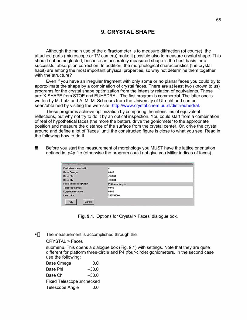
68

9. CRYSTAL SHAPE

Although the main use of the diffractometer is to measure diffraction (of course), theattached parts (microscope or TV camera) make it possible also to measure crystal shape. Thisshould not be neglected, because an accurately measured shape is the best basis for asuccessful absorption correction. In addition, the morphological characteristics (the crystalhabit) are among the most important physical properties, so why not determine them togetherwith the structure?

Even if you have an irregular fragment with only some or no planar faces you could try toapproximate the shape by a combination of crystal faces. There are at least two (known to us)programs for the crystal shape optimization from the intensity relation of equivalents. Theseare: X-SHAPE from STOE and EUHEDRAL. The first program is commercial. The latter one iswritten by M. Lutz and A. M. M. Schreurs from the University of Utrecht and can beseen/obtained by visiting the web-site: http://www.crystal.chem.uu.nl/distr/euhedral.

These programs achieve optimization by comparing the intensities of equivalentreflections, but why not try to do it by an optical inspection. You could start from a combinationof real of hypothetical faces (the more the better), drive the goniometer to the appropriateposition and measure the distance of the surface from the crystal center. Or, drive the crystalaround and define a lot of ”faces” until the constructed figure is close to what you see. Read inthe following how to do it.

!!! Before you start the measurement of morphology you MUST have the lattice orientationdefined in .p4p file (otherwise the program could not give you Miller indices of faces).

Fig. 9.1. ‘Options for Crystal > Faces’ dialogue box.

•fi The measurement is accomplished through the

CRYSTAL > Facessubmenu. This opens a dialogue box (Fig. 9.1) with settings. Note that they are quitedifferent for platform three-circle and P4 (four-circle) goniometers. In the second caseuse the following:Base Omega 0.0Base Phi –30.0Base Chi –30.0Fixed TelescopeuncheckedTelescope Angle 0.0

69

Eyepiece Rotation 0.0In the case of a platform goniometer see page 4-4 in the SMART manual (these settingsusually appear as default).

Fig. 9.2. ‘Crystal Faces’ window.

After acceptance of the settings the ‘Crystal Faces’ window is opened (Fig. 9.2). In thebeginning the list is empty. Unless by some miracle (or previous measurements on anoptical goniometer) you know the shape of your crystal, skip it by pressing OK whichbrings you to the final window (Fig. 9.3) in which the shape will be presented graphically.Of course, in the beginning this window is empty too, and do not expect to see yourcrystal before you define a closed polyhedron.

Fig. 9.3. SMART screen showing crystal habit and faces (original colors).

Here you can use various shortcuts (described at the top of the window) to analyze theshape. For example, you can rotate the picture around the phi axis using the left and rightarrow keys and rotate around chi (not omega as written on the screen, which is valid fora three-circle diffractometer) using the Page up and Page down keys. It is also possibleto rotate the picture by moving the mouse with the left button depressed.

70

All the time the program automatically finds Miller indices of the plane that can be seenhorizontal in your microscope and is oriented upwards. Thus, to measure the distance ofthe plane from the center of the crystal you should turn the scale in the microscopevertical.While the Faces window is activated you can drive the goniometer angles manually fromthe manual box. Normally you need just phi and chi (for a P4 goniometer). Choose thecircle with a button in the lower left of the box and drive it by the right-side buttons forforward and backward, slow and fast rotation. When a plane is in the proper position -horizontal in the microscope and pointing upwards - press the AXIS PRINT button; thisdisplays the Miller indices of the plane together with the corresponding angles in thelower part of the screen. The plane can be entered in the list and displayed graphically onthe screen if you now press Enter. You are asked about the plane indices first; here youcan enter the correct value for the plane distance from the center of crystal. The distanceshould be in mm, so do not forget to convert the reading from the microscope scale. Thescale in our microscope has been calibrated by a precision micrometer, and theconversion table for the microscope reading can be found at the operator place.

Tip: If the screen picture of your crystal is too small, multiply all crystal dimensions by a factorof 5 or 10. This really helps! But do not forget to re-scale to the true dimensions beforeyou finish. Otherwise, the wrong dimensions will be written to the .p4p and .ini files.

With the other shortcuts you can perform the following operations:- CNTL+F (Ctrl+F) brings up a window where you can enter the Miller indices of a plane,and then the goniometer will orient the plane/face to the measuring (i.e. upward) position.If for any reason the chosen plane is not clearly visible you can try driving to the facewith all of the signs for the indices reversed. The desired face will then be orienteddownward and maybe this position will be better.- HOME opens the face list window where you can edit face data (e.g. if you haveparallel faces on your crystal you can just add the second after you have measured thefirst).- INS toggles between a full projection of the crystal (showing also the back faces) and afront projection where face indices are displayed too.- END drives the goniometer so that the resulting view in the microscope should be thesame as the screen picture.- ESC exits the Faces menu.The display on the screen allows you to see how realistic your crystal description is. Itrotates with the crystal and gives a view corresponding to what could be seen throughthe microscope.12

On exit the face list is saved to the smart.ini and .p4p file. Naturally, if you later invokeCRYSTAL > Faces again, the list will be restored from these files.Very likely you will make a hard copy of the screen showing your crystal. A negative ofthe standard display (with a white background) would be preferable. For this you shouldleave the Faces menu (don’t worry, the picture of your crystal will not disappear) and goto EDIT > Config > Colors. Choose PRINT.LUT as the ‘Color table filename’ and there (Fig.9.4) you are! Finally run FILE > Print, or FILE > Save, or both, and do not forget to change‘Color table filename’ to the '$default' when you are done.

12 This is one of the smartest parts of SMART.

71

Fig. 9.4. SMART screen showing crystal habit and faces (a negative of the standard displaywith screen contrast and brightness further adjusted using Ctrl+T shortcut).

Tip: Crystal shape is not very legible with the default Color table in use. In order to improve thepicture you can leave the Crystal faces window and:- adjust contrast and brightness to get white lines on black background, or- use Color table filename PRINT.LUT to always see black lines on white background(contrast and brightness adjustments are also needed), or- play a game with the colors in EDIT > Colors or CRYSTAL > Faces menu. The colors aredefined using the RGB (red, green, blue) convention, for example, 000000000 meansblack, 255255255 is white, 255000000 is red, 255000255 is violet, etc.

Tip: If you decide to use another instrument, like an optical goniometer, for crystal faceindexing and measurement, then you can add face description directly to the .p4p file(which is also in ASCII) using any text editor. The format is:FACE 0.00 -1.00 1.00 0.055FACE 0.00 1.00 -1.00 0.055… etc.

i.e. the format is identical to that in the ‘Crystal Faces’ window (Fig. 9.2). Type in these lines justbefore the reflection list. In this way you can save some time and avoid typing errors whenusing XPREP for face-indexed absorption correction.

72

10. SHELXTL PROGRAMS

The SHELXTL suite consists of several major modules of which XPREP (program forreciprocal space exploration) should be used first.

The last version of XPREP should be available from the official BRUKER site as a part ofthe SHELXTL suite. However, to obtain an up-to-date (demo, but fully functional) version (thelatest one is 6.13), you can go to the web site: http://shelx.uni-ac.gwdg.de/axs/. In that caseyou need to specify user "axs"; and give the password (7 characters), which is the lasthexagonal space group (no. 194) in the International Tables (note that UNIX is case sensitive!).

XPREP performs automatic crystal system and space group determination, absorptioncorrections, scaling and merging of different data sets, index transformation, reflectionstatistics, etc. XPREP reads the raw data file namem.raw and the parameter file namem.p4p,both written by SAINT. XPREP also prepares the command file, name.ins, and reflection datafile, name.hkl, which are needed to run the other SHELXTL programs. In addition, all operationsare logged to the name.prp file, while some experimental data are written (in CIF format) into thefile name.pcf. At the end of the structure refinement the last file should be combined with thename.cif file.

!!! If you are repeating XPREP for some reason (and this happens quite frequently), do notforget to change the name of the previous .prp file before you start. It would beoverwritten, and in this way much important information about what you have been doingis lost just because you wanted to change a small thing in your data!

When you start SHELXTL, open a New project for the last time. At the very beginning youhave to choose between the “normal” and huge version. The normal XPREP works with up to450,000 reflections, which is usually enough, even for very large structures. If you haveproblems starting XPREP from the SAINT+ or SHELXTL window, very likely some systemvariables are not set properly; copy the program to the current working directory and run itdirectly (double click on the program name or from Windows ‘Run’ command).

XPREP is an easy to use, essentially interactive and menu-driven program. At each stepthe program presents all available information, selection of possible answers and therecommended choice. Just read the screen output carefully. However, we strongly recommendgoing trough the SHELXTL manual, pp. 4-1 to 4-25, and examples listed there.

!!! It is very important to note that if any ambiguity exists about the space group, you shouldassign different filenames (.ins and .hkl) for the data prepared in each space group.Then the options have to be considered and tested (through XS or any other structuresolving program) during future work before making a final choice. Usually a CFOM ofless than 5 is a decisive indication that the proposed space group is correct, and avalue grater than 10 is rather unlikely for the correct space group. Chances of successcould be increased if you accept one of the probable space groups, then performabsorption corrections and repeat the space group determination. (If the Laue class ischanged, remember to perform absorption corrections using the true Laue class andinitial data set.)

When you run XPREP, the program asks for name.raw (beware, extension .hkl isassumed)13 and format of input/output files; then checks (preliminary) the lattice centering.

13 It means that one can run XPREP using any .hkl file as input; useful if you want to check/re-check yourdata.

73

After that you will see the main menu, which, depending on the stage, should be more or lesssimilar to Fig. 10.1.

If you follow the program’s own suggestions for the sequence of data preparation stepsyou will be guided through the usual necessary operations (checking the reduced cell and apossible higher lattice symmetry, determination of the space group extinctions, calculation ofthe reflections statistics, a suggested unit cell content with determination of calculated densityand linear absorption coefficient, as well as preparation of the .ins and .hkl files). So, in atypical XPREP run you will follow the order:

[H] Search for HIGHER metric symmetry,[S] Determine or input SPACE GROUP,[D] Read, modify or merge DATASET,[C] Define unit-cell CONTENTS,[F] Set up shelxtl FILES,[Q] QUIT program.

Be ready to see many submenus and sub-submenus and to make proper choices or input somerequested data. Fortunately, the default options indicated by XPREP are the best choices inmost cases.

Fig. 10.1. XPREP window showing the main menu.

Keep on hand the chemical composition of your crystal, you need it for option ‘C.’However, if the chemical formula was entered at the time you defined the current project inSMART (Crystal > New Project, Crystal > Edit Project, etc. Fig. 2.1) XPREP will extract thechemical composition from the .p4p file. In step ‘C’ the program calculates some very importantdata: Mw, Z, Dx, non-hydrogen atomic volume, F(000) and m. All of them should havereasonable values for your sample; consult an experienced person if you are in doubt.

Tip: In many cases the non-hydrogen atomic volume should be about 16 Å3, but it can be aslow as 12 Å3 when only very light atoms are present. Conversely, for compoundscontaining numerous heavy atoms the volume can even reach 25 Å3.

74

In cases of high (tretragonal or above) symmetry it is a good idea to test for merohedraltwinning, option ‘M’, somewhere in the XPREP run.

Before the last step and after the cell content description, it is highly advisable to apply anabsorption correction, but for this you have to take your own initiative and choose from theprogram menu. Different absorption corrections are described in chapters 4.7 and 4.8 (pp. 4-21to 4-23) of the SHELXTL manual. In XPREP they are hidden under option ‘A’ and should be runbetween ‘C’ and ‘F’. There are two options:

- FACE-indexed absorption correction, input ‘A’ then ‘F’,- PSI-scan absorption correction, input ‘A’ then ‘P’.The second option also includes correction for laminar (plate-like) crystals.Pay attention to the intensity agreement index, Rint, before and after absorption

correction. The value of Rint should be significantly lower after correction. Do not forget tocalculate the new reflection statistics after the correction. Press or confirm in sequence:

‘D’ Read modify or merge DATASET,‘S’ Display intensity STATISTICS,‘A’ Merge ALL equivalents …,

then compare the columns R(int) and R(sigma) before and after correction. The correspondingtables are also logged into a .prp file.

Here, we emphasize that a face-indexed absorption correction is preferred from aphysical point of view. Read more about this and detailed instructions in the “Notes onAbsorption Correction” below.

It is important to note that the quality of correction depends also on the accuracy of theabsorption coefficient applied. It is set up in the definition of the unit cell content in XPREP andthis should be checked carefully (both the chemical composition and the Z number). Sometimesthe structure solution might show that your assumption about the chemical composition was notcompletely right, and then it is advisable to repeat the absorption correction with the newabsorption coefficient calculated for the correct chemical formula.

For area detector absorption and other corrections it is also possible to use a separateprogram, SADABS, described later in chapter 11. If you wish to combine a face-indexedcorrection in XPREP with SADABS (which is a common sequence) remember to answer "Y",when the question 'Copy whole of input file with updated I and sigma(I) [N]' appears during theface-indexed correction. By default the file obtained has the extension .abc and is suitable forinput into SADABS.

!!! At the end of an XPREP run (option ‘F’) do not accept the default answer when thequestion ‘Do you wish to (over)write the intensity data file name.hkl ? [N]’ appears. Typein ‘Y’(es), otherwise a new .hkl file will not be written.

After the run inspect the XPREP log file name.prp. This file contains all XPREP results.The XPREP output file “name.ins” can be directly submitted as input for crystal structure

determination by direct methods.Among the numerous XPREP features ‘RECIPROCAL space displays’ (option ‘R’),

‘Contoured PATTERSON Sections’ (option ‘P’) or ‘Generate powder pattern’ (option ‘D’ from mainmenu, then option ‘G’ from submenu) should be noted as being very helpful (e.g. for checkingthe lattice symmetry, during structure solution by the heavy-atom method, or if you had enoughmaterial to collect a powder diffraction pattern). The ideal powder pattern will be generated ifyou submit an .ins or .res file as input for XPREP.

The other programs listed below will not be described in detail. We assume that you arean experienced user of the SHELX programs that have been around in so many versions forover 30 years. Of course, you can use a name.hkl file prepared by XPREP and any other

75

program for crystal structure solution and refinement. Just remember that the name.hkl filecontains F 2 (not F) and corresponding sigma values.

XS is the program for structure solution by direct methods or Patterson synthesis.XL is the least-squares structure refinement program.XP is the program for interactive molecular graphics.XCIF is the program for preparing tables for publication from CIF.XPS is the program for structure solution by fragment search.XPRO is the interface for protein applications.XWAT is the program that performs “automatic water divining” for macromolecules.

Tip: Try to solve your structure by direct methods if the crystal consists of light atoms only(organic compounds) or if the crystal contains many heavy atoms (that could havedifferent atomic numbers). Try to use the Patterson (heavy atom) method if you have oneor two atoms that have significantly higher atomic numbers than other atoms. Directmethods are usually more successful for noncentrosymmetric, the Patterson method forcentrosymmetric structures.

For beginners and crystallographers with not so much experience with the SHELXTLprograms we recommend “Allen Hunter’s Youngstown State University X-ray StructureAnalysis Lab Manual: A Beginner’s Introduction”. The manual is available (in the form of a .pdffile) from the web site: http://www.as.ysu.edu/~adhunter/YSUSC/index.html. Some workedexamples can also be found at the same site.

Instead of the SHELXTL suite some of us readily use OSCAIL, a program systemdeveloped by P. McArdle, Crystallography Centre, Chemistry Department, NUI Galway, Ireland(J. Appl. Cryst., 1995, 28, 65). The latest version is always available from the web site:http://www.nuigalway.ie/cryst/software.htm.

An excellent integrated system, WinGX, of publicly available Windows programs for thesolution, refinement and analysis of single crystal X-ray diffraction data collected andconnected by L. J. Farrugia, Department of Chemistry, University of Glasgow, UK (J. Appl.Cryst., 1999, 32, 837-838) is available at the INTERNET address:http://www.chem.gla.ac.uk/~lous/software/wingx.

76

11. ABSORPTION AND OTHER CORRECTIONS BY SADABS

This chapter contains suggestions for the use of SADABS V2.07. As a result of manyimprovements and fine tuning this version gives lower Rint values, especially for highlyabsorbing crystals (but not always better refinement results). Instructions were mainlyprepared by Dr Gene Carpenter, but some additional explanations are taken, more or lessdirectly from the SADABS help file.

The latest version of SADABS should be available from the official BRUKER site.However, to obtain the fully functional demo version, you can also go to the web site:http://shelx.uni-ac.gwdg.de/axs/. In that case you need to specify user "axs"; and give thepassword (7 characters), which is the last hexagonal space group in the International Tables(note that UNIX is case sensitive!). The help file (SADABS.htm) prepared by George Sheldrick isavailable, too.

The accessory program GSView must be available to run in the middle of a SADABS run.GSView (freeware) is able to view and print (even on a non-Postscript printer) postscript andencapsulated postscript files (extensions .ps, and .eps) prepared by SADABS or otherprograms. An .exe file for installing GSview is provided in the win directory of Sheldrick’s site,but the program can be downloaded from many different places (try Yahoo or Google search).

SADABS can correct for diverse kinds of experimental errors, like variation of theirradiated volume of the crystal, incident beam inhomogeneity, absorption by the crystalsupport, crystal decay, etc. SADABS also improves the s.u.s of the intensities. SADABS worksusing data present in .raw (or .abc)14 files and, except for an interactive screen input, no otherdata, files or variables are required.

It is important to start with properly prepared .raw files from SAINT for the individual runs,with none of the fudges that SAINT can apply. In particular, no correction for decay, noinstrument error, and no correlation filter should have been used (but you already knew that, ifyou read chapter “Data reduction strategy” carefully). The program functions by comparingreflections that should have the same intensity, either equivalents or the same reflectionrecorded at different instrument angles; hence, high redundancy much improves SADABSresults; all available data should be used (avoid the FILTER option in SAINT). It is also possibleto perform an additional absorption correction for a spherical crystal.

The namem.raw or namet.raw file may be read instead of the individual scans, butnamet.raw is not recommended since SADABS can scale better, and rejecting reflectionsprematurely screws up the statistics. There is no disadvantage in reading namem.raw insteadof the individual scans, since the namem.raw file traces run numbers and any series of scanscan be excluded in the next SADABS run if there is a good reason for it (e.g. if that series ispoorer than the rest of data).

In order to function correctly, SADABS requires the Laue class for the crystal. If thechoice is uncertain at this stage, you will have to pin it down with the use of XPREP operatingon a .raw file.

The program proceeds by first making a preliminary pass through the data, and thenadjusting parameters to achieve improved plots of several quantities against resolution orintensity. This is the reason why GSView must be available. It is also useful to review thedocumentation as you proceed, because otherwise it is hard to tell what is going on.

There is a possibility that the new SADABS cannot be run from the SAINT+ menu, but hasto be run from its own directory (consult the system administrator). In that case a complete pathmust be given for any files it uses. This is easier than it sounds, because you can find the

14 An .abc file is a copy of a .raw file containing among other data corrected intensities and their s.u.s; it isprepared by XPREP during a face-indexed absorption correction.

77

previous lengthy path by pressing the up-arrow repeatedly, and then editing the rightmost partto specify the intended file. It is much better to start SADABS from the SHELXTL menu. Thethird, very simple way used in our laboratory to run SADABS is: copy the program into theactual working directory (directory containing your data) and run SADABS.exe.

During the SADABS run carefully read the screen outputs and follow the question andanswer format. The SADABS questions are marked by the usual •fi sign, and defaultanswers are given in brackets. (Only parts of some long questions are given in the followingtext.)

Step 1. Refinement of parameters to model systematic errorsThis step involves data input and modeling of absorption and other systematic errors.

•fi Maximum number of reflections allowed [500000]

The number of reflections is not limited, but the default number is more than enough forordinary structures!

•fi Enter listing filename [sad.abs]

When prompted, give a name for the log file that easily identifies your crystal. If you omitthe extension, “.abs” is added automatically. The program then shows a list of Lauegroups.

!!! Select the correct Laue group from the list.•fi Test Friedel opposites … [Y]

The usual answer to this question is 'Y'. If the redundancy is high and if you know whatyou are doing enter 'N', but this answer halves the data to parameter ratio fordetermination of program parameters. If you answer 'N,' it is further necessary to definethe point group so that Friedel opposites can be correctly defined.

•fi Enter filename (/ if no more) [ ]

The input files are name0.raw, name1.raw, name2.raw (and perhaps more); the “.raw” isadded automatically if you omit it. The merged (namem.raw) file can also be used. Asnoted above find the path if necessary, then replace name.abs with name# (or namem).Successive data files appear automatically.The program now reads and briefly checks your data, and prints some characteristicparameters. Pay attention to the redundancy and mean(I/sigma) tables. The determinationof a model for the systematic errors starts now and some thresholds should be specifiedfor excluding some reflections from the parameter refinement. (These reflections may stillbe corrected and included in the final output .hkl file).

!!! Accept defaults (given in brackets) for the first pass!•fi Enter mean(I/sigma) threshold … [3]

… but threshold could be lower (2.5 or even 2) if reflections are exceptionally weak.•fi Highest resolution for parameter refinement [0.1]

This small default value 0.1 excludes none of the data in the model fitting, and is a goodplace to start.

•fi Factor g for initial weighting scheme … 15 [0.04]

Note that a more precise value of g is determined later in step 2. However, if the newvalue is very different from 0.04, this stage should be repeated.

•fi Restraint esd for … [0.005]

15 w = 1/ [s 2(I)+(g<Ic>)2], where <Ic> is corrected mean intensity.

78

This value is almost always in the range 0.002 to 0.005, but could be higher in the case ofhighly absorbing samples; the best guide is appearance of the Postscript plot (see theexplanation below).

•fi Suitable spherical harmonics orders … [6, 3]

… in the case of moderate absorption, but should be [4, 1] for weakly, and [8, 5] forstrongly absorbing crystals.

•fi Special treatment of plate-like crystals [N]

It seems that this option does not work, at least in versions 2.03 and 2.05! In a limited testusing version 2.03 answer Y(es) always resulted in a small increase in the finalagreement indices.

•fi Number of refinement cycles [15]

Sometimes it helps to increase this number to 20. The program then prints the number ofreflections employed, effective data to parameter ratio, the initial value of R(int), refinesparameters against the selected data, and reports the resulting value of R(int). Normally,you accept (option A) this result and proceed to the next step.

•fi Repeat parameter refinement (R) or accept (A) [A]

Step 2. Reject outliers and establish error modelThe error analysis continues and 'correct' standard uncertainties (s.u.) for the correctedintensities are derived, using some of the results from Step 1.

•fi High resolution limit [0.10]

This value is usually, but not necessarily the same as in Step 1. Remember that onlycorrected reflections satisfying this condition will survive, i.e. they are written in thesad.hkl file.

•fi |I-<I>|/su ratio for rejection [4.0]

Very likely reflections with |I-<I>|/su > 4.0 suffer from serious systematic errors.•fi g-value … used for rejections16 [0.04000]

If the number of unique reflections left after the |I-<I>|/su test looks reasonable, accept theparameters used.The program now calculates a new g-value, which gives the best error model and shouldnormally be accepted. A table of tentative results appears next; once again choose‘accept,’ because there will be an opportunity to try changes later. But if the resultsindicate that a particular scan is much worse than the others, do not forget to leave thisscan out when you repeat the whole calculation.

Step 3. Output Postscript diagnostics and corrected dataThe diagnostic plots prepared in this step are essential for verifying that the parametersin the error model have been correctly adjusted.Write Postscript diagnostic file (Y or N) [Y]Name the diagnostic file something like name_n.eps (perhaps with a full path) whenprompted. If you omit the extension, “.eps” is added automatically. The “n” after name is aserial number, because you will likely make more than one trial. Also give a short title thatwill appear on each page of the diagnostic file.

16 g-value for use in: su2 = k [s 2(I) + (g<I>)2], where k is a scaling factor. s (I) originally comes from SAINT,but in the final stage I is substituted for Ic, where Ic is the corrected intensity.

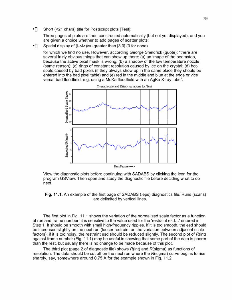
79

•fi Short (<21 chars) title for Postscript plots [Test]:

Three pages of plots are then constructed automatically (but not yet displayed), and youare given a choice whether to add pages of scatter plots:

•fi Spatial display of (I-<I>)/su greater than [3.0] (0 for none)

for which we find no use. However, according George Sheldrick (quote): “there areseveral fairly obvious things that can show up there: (a) an image of the beamstop,because the active pixel mask is wrong; (b) a shadow of the low temperature nozzle(same reason); (c) rings of constant resolution caused by ice on the crystal; (d) hot-spots caused by bad pixels (if they always show up in the same place they should beentered into the bad pixel table) and (e) red in the middle and blue at the edge or viceversa: bad floodfield, e.g. using a MoKa floodfield with an AgKa X-ray tube”.

View the diagnostic plots before continuing with SADABS by clicking the icon for theprogram GSView. Then open and study the diagnostic file before deciding what to donext.

Fig. 11.1. An example of the first page of SADABS (.eps) diagnostics file. Runs (scans)are delimited by vertical lines.

The first plot in Fig. 11.1 shows the variation of the normalized scale factor as a functionof run and frame number; it is sensitive to the value used for the 'restraint esd…' entered inStep 1. It should be smooth with small high-frequency ripples. If it is too smooth, the esd shouldbe increased slightly on the next run (looser restraint on the variation between adjacent scalefactors); if it is too noisy, the restraint esd should be reduced slightly. The second plot of R(int)against frame number (Fig. 11.1) may be useful in showing that some part of the data is poorerthan the rest, but usually there is no change to be made because of this plot.

The third plot (page 2 of diagnostic file) shows R(int) and R(sigma) as functions ofresolution. The data should be cut off on the next run where the R(sigma) curve begins to risesharply, say, somewhere around 0.75 Å for the example shown in Fig. 11.2.

80

Fig. 11.2. An example of the third plot from SADABS diagnostics file.

Fig. 11.3. An example of the fourth plot from SADABS diagnostics file.

The fourth plot (Fig. 11.3) shows the mean |E2-1| versus resolution. For large organiccompounds the curve should be close to the 0.968 line for a centrosymmetric, or close to the0.736 line for a non-centrosymmetric structure. For coordination compounds containing heavyatoms and for compounds with heavy atoms in special positions the plot is less reliable.

The fifth and sixth plots (page 3 of .eps file) show chi-squared as a function of resolutionand of intensity (Fig. 11.4). If the parameters have been correctly adjusted, both should benearly flat around one; the g-parameter may occasionally need to be increased if the plots driftaway from unity at high intensities. It is not unusual to see deviations from unity at lowresolution.

81

Fig. 11.4. An example of the third page in SADABS diagnostics file.

It is advisable to print out the plots for easier comparison with later trials. This is donedirectly from GSView. Set proper paper size (Media > Letter or A4), and then print using theFile > Print command. It is necessary to mark a suitable printer driver (‘Device’) in the Printersetup dialogue box. Read ‘Help’ in order to make the proper choice, but the mswinpr2 driveruses the Windows printer drivers and should work with any printer with raster capabilities.

Usually you should repeat (R) the whole calculation at least once, with a new resolutionlimit, the best g-value so far, and, possibly, with particular scans left out. The g-valuemay need yet another cycle of adjustment, but it is not easy to achieve any furtherimprovement.

•fi Repeat (R), write .hkl file (W), or quit (Q) [W]

Finally, when the plots look as good as possible, write (W) the corrected data to a filename.hkl (or sad.hkl, if you only confirm the default name). This file is in HKLF 4 format,i.e. contains F2 and s 2(F). You may also supply the value of m¥ r to apply an overallisotropic absorption correction; r is the effective crystal radius, weighting the smallestdimension more heavily.

•fi Enter name of output .hkl file [sad.hkl]

•fi Mu*r of equivalent sphere for additional sphericalabsorption correction. Enter <CR> if none:However, we never have obtained any improvement when using this additionalcorrection and the previous SADABS versions. Actually, the results were nearly thesame with and without the correction. Version 2.07 has not been tested yet.

82

The last question means that data will be corrected for l/2 contamination. The defaultvalue is suitable for a sealed-tube Mo Ka SMART diffractometer.

•fi Lambda/2 factor [0.0015]

but submit the correct value if your system is calibrated (see sadabs.htm file forsuggestions how to do it; the value should depend on the tube voltage).

After the SADABS run check the log file which contains most of the screen outputs youhave already seen, and some other useful data, but only the ratio of minimum to maximumapparent transmission (Tmin and Tmax, respectively). So, how to get these very popular andoften quoted numbers? In SHELXL input the crystal dimensions using the SIZE command and incombination with the ACTA command you will find the Tmin and Tmax values in CIF. If their ratio isequal to the ratio listed in the SADABS log file, then everything is OK. If not, stay cool, nobodycares, except perhaps referees of some journals, especially of Acta Crystallographica.

To combine SADABS with a face-indexed correction you should run the face-indexedcorrection first. The procedure is to integrate with SAINT, use XPREP to apply the face-indexedcorrection to the .raw file, and then feed the corrected file to SADABS. In XPREP be sure to say‘yes’ when asked whether to copy the complete data file with corrected intensities and sigmas– it is the file you want to use with SADABS. (By default it is named with the extension .abc.)Then use SADABS with m¥t = 0 to do the other corrections and merging.

Important note: When data are corrected with SADABS then the experimental absorptioncorrection type should be defined as ‘multi-scan’.

Tip: Even if you don’t want to use SADABS for scaling your data, George Sheldrick suggestsyou run the program in order to get and analyze diagnostic plots (…“they may revealmore than you are expecting”…). We must agree with this.

83

12. NOTES ON ABSORPTION CORRECTIONS

A short but very informative overview of different methods and programs used forabsorption correction has been prepared by Louis J. Farrugia; it is available as help files('absorb.htm' and 'abs100.htm') distributed with the WingGX suite mentioned above [L. J.Farrugia, J. Appl. Cryst., 32, 837-838 (1999)].

The first part of this chapter is mainly based on this summary, which with some minorchanges is reproduced here with the author’s permission.

For most crystals containing elements heavier than the first row transition metals, it islikely that absorption is the single most important contributor to the systematic errors. Acorrection for absorption is usually required in such circumstances and is mandatory for anActa Crystallographica submission. [Note: If the ratio of predicted transmission factorsTmax/Tmin is bigger than 1.10, the checkcif procedure generates the alert: “An absorptioncorrection should be applied". Predicted transmission factors are a function of crystaldimensions, linear absorption coefficient, m, maximum theta value during data collection, qmax

and type of radiation.]There are several options for absorption correction [1]17. The refined parameters

principally affected by systematic errors due to absorption are the anisotropic thermalparameters, more appropriately called anisotropic displacement parameters (a.d.p.s) [2].Because absorption primarily affects the low angle data, the net result is that the Ui j tensorrefines to a smaller value than the "true" value. In severe cases, it may even result in negativeeigenvalues (i.e. a non-positive definite Ui j tensor).

There are three basic methods for applying absorption correction to reflection data. Indecreasing order of theoretical rigor they are:

1. Exact numerical corrections (i.e. analytical, Gaussian quadrature, spherical, cylindricaland needle),

2. Semi-empirical corrections (i.e. psi-scans, CAMEL-JOCKEY and multi-scan),3. Refined corrections (i.e. DIFABS, XABS2, SHELXA).1. Numerical methods. These methods provide mathematically exact absorption

corrections, providing of course that the input data are correct. It is generally agreed that thebest absorption corrections are provided by the analytical [3] or Gaussian quadrature [4]methods. These two methods require that the crystal faces are well defined and can beaccurately indexed and measured. These conditions are not often met. It can be time consumingto index a specimen with numerous faces and difficult to measure accurately the distancesbetween faces. For these reasons, numerical methods are used less often than those whichare easier to implement experimentally. In cases of severe absorption, however, they are theonly really effective methods. The spherical and cylindrical corrections also provide numericallyaccurate corrections for crystals adopting the requisite morphology, but are less useful, sincegrown crystals are not usually spheres or cylinders. Crystals may be ground to spheres, butmany materials do not survive such treatment.

2. Semi-empirical (or in short ‘empirical’) methods. These methods provide an approximatecorrection, based on an experimentally determined absorption surface. The semi-empiricalmethods rely on making extra intensity measurements.

The multi-scan method of Blessing [5] is of most use when there is a large redundancy inthe data-set. Equivalent intensities are analyzed in terms of a multi-polar spherical harmonicexpansion and the method is implemented in the programs PLATON [6], SORTAV [7] andSADABS [8]. This program requires the data set to contain an extensive set of equivalents, andis primarily of interest for data collected using area-detectors, which routinely have a large

17 References for this chapter are listed at the end of the Guide (see Literature).

84

degree of over-determination (redundancy). It models the absorption surface using a sphericalharmonic series based on differences between equivalent reflections and will probably not bevery effective for triclinic and monoclinic crystal systems (since these have fewerequivalents).

A somewhat similar method called CAMEL-JOCKEY [9] uses a trigonometric seriesexpansion of the diffractometer angles, but is little used since so many more experimentalmeasurements are required.

The method most commonly used with scintillation counters is the azimuthal scan or psi-scan method of North et al. [10]. This is the simplest method, involving the measurement of theintensities of a (usually small) number of reflections with chi values close to 90° at different psi(phi) values. An averaged absorption surface is thus computed and used to calculate thetransmission factors. It works remarkably well, but is unsuitable for crystals with large m¥rvalues. [Note: In checkcif procedure, if m¥tmid is bigger than 3.0 (tmid = medial crystal size), youwill receive the message: "Alert A Crystal and compound unsuitable for non-numericalcorrections”.]

3. Refined corrections. These methods are the least scientifically valid methods, in thatthey require a refined model (hence the structure must be solved and isotropic a.d.p.s shouldbe known), and provide a "correction" for the data based on the assumption that anyconsistent differences between the calculated and observed structure factors are due toabsorption.

This type of absorption correction, the so-called refined corrections: DIFABS [11], XABS2[12] and SHELXA [13] have fallen out of favor in the recent past. The various programs differ inthe exact mathematical functions used to model these differences, but all suffer from the samephilosophical problem, in that the data are being modified to fit the model.

Use them to discover discrepancies between calculated and observed structure factors.If “corrections” are significant, then you can suspect the quality of previous absorptioncorrections. Remember that refined corrections are based on a very simple hypothesis. Checkeverything: experimental data, structural model and try another correction program.

All methods and programs mentioned are available in the WinGX suite. Some of them arediffractometer specific (Enraf-Nonius CAD-4), but some require only name.ins, as well asname.hkl and/or name.fcf file and Bruker users can employ them with no problems. In somecases it is necessary to run SMART-SAINT Import Utility (DATA > SMART-SAINT) to convertand concatenate SAINT .raw files first (default file name is concat_hkl.sortav). Then use thisfile as input in the DATA > KappaCCD > Process Data menu, where you can perform empiricalSORTAV or Gaussian quadrature corrections for absorption. We have no experience with datacorrection programs available in WinGX, but if you are desperate … Anyway, let us know if theresults are extraordinary. A comparison of different methods using Na2WO4•2H2O with m(MoKa) ª 19 mm–1, as a model crystal is also given in the absorb.htm file.

As you already know from the previous chapters Bruker AXS Pack offers severaloptions for absorption corrections. They are: numerical (face-indexed, Gaussian in XPREP) andempirical (psi-scan in XPREP, multi-scan in SADABS) corrections. This should be enough, sincethe refined corrections cannot be recommended in any event.

It is, first of all, necessary to learn how to recognize “good” or “suitable” absorptioncorrections. Several parameters are generally utilized for this purpose. They should always becombined, otherwise you can easily come to the wrong conclusion. The parameters are listedin order of appearance and approximately increasing importance. It is assumed that your .hklfile contains the complete set of reflections, including all collected equivalents.

1. Rint and/or Rs values. Most programs for crystal structure solution and refinementcalculate these values. Of course, in a typical procedure you will already have compared thevalues in an XPREP or SADABS run. If after correction the values are not significantly lower,something is wrong with your data or with the applied corrections. In a “good” correction, youcould expect that Rint/Rs values will be halved, and even more gain is possible in case of high

85

redundancy and high linear absorption coefficient. However, there is no simple or linearrelationship between Rint/Rs and final agreement indices, meaning that, for example, a lowerRint value does not always result in a lower R1 value. SADABS almost always gives the lowestRint/Rs values no matter whether the other indices are the best or not.

2. Transmission factors, Tmin and Tmax. If the values are close to each other and/or closeto 1, the correction is very likely insignificant. Too small values are not promising; see below(“Psi-scan corrections”) what to do. The values of Tmin and Tmax and/or their ratio should beclose to the values predicted from crystal dimensions. Those “theoretical” values will becalculated by SHELXL if you add the SIZE and ACTA commands to the .ins file or in the checkcifprocedure. However, we do not see any good reasons why Acta Crystallographica editorsinsist on such theoretical values, since they do not account for specific experimental detailsand the exact crystal shape.

3. Number of inconsistent equivalents. It is easy to check this number since it is given inevery SHELXL .lst file. As a rule, a smaller number means better correction, although, onceagain there is no direct relationship between the number of inconsistent equivalents and final Rfactors. As usual, SADABS is the best in this sense, very often giving zero number ofinconsistent equivalents, but not always the best corrections as measured by the final results.

4. Weighting scheme. In ordinary circumstances the first parameter in the weightingscheme (WGHT) is small (less than 1) and the second one tends to zero. If the secondparameter is 5, 10 or even bigger, carefully re-check your data. One possible reason for sucha high value could be inappropriate absorption correction. Unusual weighting schemes areoften seen when the data have been corrected by SADABS.

5. Final agreement indices (R1, wR2, etc.) and residual peaks in DF map. These indicesare always strongly correlated and any one of them can be used as a reliable indicator forgood corrections. If the sample contains very heavy elements it is not unusual to see residualpeaks of up to ca. 4 e Å–3 even with a satisfactory absorption correction. Do not panic, withoutcorrections such peaks could be as high as 10 e Å–3!

6. The ultimate and probably the most important sign of a good absorption correction areatomic displacement parameters (a.d.p.s). On the other hand, in ordinary and non-problematiccases they attract little attention. According to L. J. Farrugia (see above): “The acceptedwisdom is that absorption errors cause the a.d.p.s to be somewhat smaller and moreanisotropic than the "true" values (in this context the "true" value is assumed to be that obtainedfrom the analytical correction)”. The main problem with a.d.p.s is: how to estimate the “true”values if it is not possible to perform a face-indexed correction. Namely, a list containingstandard a.d.p.s, which would be similar to the list of standard (average) bond distances andangles, does not exist. And, if the “true” values are already known from the analyticalcorrection why would you be interested in something else? An additional problem is that formiddle to high absorbing crystals (m bigger than ca. 15 mm–1) the analytical corrections do notalways give a.d.p.s that are the “best” in the above sense.

Anyway, if a part of the isotropic displacement parameters is small (e.g. B less than 1 Å2,U less than 0.013 Å2) and if some of the a.d.p.s later become non-positive definite you have aproblem with absorption correction. The presence of some (very) elongated thermal ellipsoidscould also be a reliable indicator of unsuitable absorption correction. However, thermalellipsoids are sometimes elongated for good chemical reasons; the list of examples andpossible explanations is long and will not be given here. In addition, elongation could be causedby static and/or dynamic disorder, twinning, etc.

Face-indexed correctionTechnically, the procedure for performing face-indexed absorption correction using

XPREP (option ‘A’, then ‘F’) is very simple, especially if description of crystal shape is alreadypresent in the .p4p file. (Accept the default value for precision only.) However, to use face-indexed corrections, one should measure the crystal shape very carefully. Every serious

86

crystallographer can tell you that this pays off. Your Rint might sometimes be worse after theapplication of this correction compared to the other types, but your data will always be morerealistic; also, refined a.d.p.s and R factors should be better and the residuals in the differencemap smaller when you do a face-indexed absorption correction. Nevertheless, if the crystal isvery small (or needle, or plate) and opaque it is very hard to index and measure its facesproperly with the Bruker optical system on the P4 goniometer. Keep in mind that the shortestdistances are the most critical! Fortunately, in this case absorption effects are not verypronounced and the other techniques may give satisfactory results.

Psi-scan correctionsEllipsoid correctionsThis method of empirical absorption correction in XPREP should give accurate results if

your crystal has an ellipsoidal-like shape. It could also do well if you have a crystal withirregular shape that has well-developed faces, provided that it is not a thin plate. It is notnecessary to collect real psi-scan data, since the program itself selects suitable sets ofreflections for refining the absorption parameters to define a pseudo-ellipsoidal surface, whichis further used to calculate corrections.

For ellipsoid corrections, you have to input the m¥r product, where m is the linearabsorption coefficient and r is one-half the mean crystal dimension. Therefore, note them value calculated by XPREP, calculate the mean crystal dimension before the run and makesure you keep cm and mm straight for both the measurements and the units of m. According tothe SHELXTL manual, during this calculation the smallest crystal dimension should be heavilyover-weighted, and at the same time the m¥r product does not need to be determined veryaccurately. According to our experience this correction is not so simple as could be naivelyconcluded reading the previous text and a very short report given in the manual. By changingthe m¥r product and some of the other parameters as described below you can attain asignificant improvement in your results. Follow the procedure:

- Chose option ‘A’, then ‘P’ and press Enter three times,- Type in 0.001 as the ‘Tolerance for direction cosines [0.00000]:’,- Confirm default values for ‘I/sigma threshold [20]:’ and

‘Resolution threshold (Ang.) [1.0]:’.After the message showing number of reflections selected for the refinement confirm E

as the default answer to the question:- Lamina (L), Ellipsoid (E) or Quit (Q) [E]:

and input actual m¥r product. Then the program calculates Rinf values before and aftercorrections. Accept the default answer to the question:

- Print intensities (Y or N) [N]:and chose R as the answer to the question:

- Process data (P), Repeat (R) or Exit (E) [P]:.Circle through the E Æ N Æ R Æ E … loop changing the m¥r product within reasonable

limits, say between 0.1 and 3.0. Generally speaking, the m¥r product should be increased forlow absorbing and decreased for highly absorbing crystals. Note the value that yields thelowest Rint.

After that choose Exit (‘E’) and repeat the whole procedure several times with different‘I/sigma threshold [20]:’ – test at least values of 10 and 30 – and ‘Resolution threshold (Ang.)[1.0]:’ – test for example values of 0.9 and 0.8. Finally, make the corrections (‘Process data’)using the combination of parameters that yielded the lowest Rint value.

Even in the case of a very large m¥r value, the psi-scan method could give good results inmany aspects. However, the resultant a.d.p.s are usually less acceptable.

87

Lamina correctionsThis empirical correction is suitable for plate-like (lamina) crystals. Start psi-scan

corrections (‘A’ then ‘P’) in the usual way and when the question- Lamina (L), Ellipsoid (E) or Quit (Q) [E]:

appears, suddenly change your mind and enter ‘L’ instead of ‘E’. The program then asks forindices of the principal face (fortunately suggesting them at the same time) and a minimumglancing angle, where the default value (3°) should be accepted. Although according to themanual, “for strongly absorbing crystals which are good approximations to thin plates, thismethod can produce spectacular improvements”, we have never obtained convincingly betterresults with it. Also, in one case of a low-absorbing sample (unfortunately the only one tested)the ellipsoid correction also gave lower R factors than lamina correction. May be we did notfind the proper combination of ‘I/sigma threshold [20]:’ and ‘Resolution threshold(Ang. ) [1.0]:’. It always turned out that we could still use the face-indexed absorptioncorrection in the case of plate-shaped crystals. The principal face Miller indices are easilydetermined, and even irregular plate shapes could satisfactorily be approximated by a selectionof planes perpendicular to the plate, or nearly so. Of course, the problem of how to measurethe crystal thickness is very important here, whereas the thickness is refined as a variable inthe Lamina correction.

SADABSThe program is specific, because, apart from absorption correction (accomplished as

described above), it should be able to solve some other absorption problems (shading by themounting glass fiber, absorption by a capillary and the solution in it, etc.), which the otherroutines are not designed to cope with. Because details on how to use SADABS are describedin the previous chapter, only a few comments will be given here.

Many, maybe the majority of Bruker users, employ SADABS, but none of them can tellyou what it actually does (with the exception of the author, of course). The users are justsatisfied that they obtain an improvement in their R values. Our experience with SADABS is notso good, since the program usually has given worse results than XPREP with an empirical (psi-scan) correction applied. However, our samples often contain very heavy elements (Bi, Pb, Tl…) in a significant, sometimes more than 50 % amount and could not be considered typical. It iswell known (George Sheldrick, private communication) that SADABS is not so good withstrongly absorbing samples (though version 2.07 is, no doubt, better).

On the other hand, refinement of the structure of glycyl-t-serine, m = 0.134 mm–1, crystalsize: 2.2¥2.0¥0.8 mm (Görbitz, 1999), showed how effective SADABS could be in reducing Rint

values even for very large crystals (e.g. crystal bigger that the collimator pinhole), especiallywhen there is great redundancy. Nevertheless, ten sets of data collected under differentexperimental conditions, with crystals of different sizes and treated/not treated with SADABSrevealed no significant variations in molecular geometry and atomic displacementparameters. These results agree with one of our studies on a large crystal (size:1.15¥0.14¥0.13 mm) with approximately ten times bigger m value.

When running SADABS you have to choose the resolution limit twice, first for theparameter refinement, and second, after inspection of the diagnostic file (Fig. 11.2), for datatruncation. At first sight it seems reasonable to input the same value (used for data truncation,of course) in both places. However, in most cases the choice does not have a significantinfluence on the results of the structure refinement. Therefore, confirm the default values (0.1)in the SADABS run and truncate reflections, if necessary, with the SHEL command duringstructure refinement by XL or SHELXL.

88

EpilogueThe aim of this chapter was to clarify the role of absorption and the corresponding

corrections in single-crystal structure analysis. If we have not been very successful and youare still confused about what to do, in future work keep in mind the following temporary 18

rules:1. In the great majority of cases absorption has no significant effect on the final atomic

coordinates (i.e. they agree within 3s limits with and without absorption correction). Therefore,bond distances and angles, as the main results of the crystal structure analysis, will be reliable,perhaps only slightly less precise, even with un-corrected data.

2. When the crystal is low-absorbing, say with m £ 2 mm–1 (maybe even more, but theupper limit still needs to be determined), in most cases absorption has no significant effect evenon a.d.p.s. Here the crystal shape is not important, the sample could be spherical, regular,irregular, plate-like or rod-like.

3. Although this could be time consuming, use face-indexed absorption correctionwhenever possible.

4. One of the Bruker fans (since our documentation is lost, do not ask for his/her name)has sent the following comment to the users list: “In limited testing, I found that for a well-defined, moderately absorbing (m about 10 mm–1) crystal of relatively anisotropic shape, aSADABS correction did rather well, a face-indexed correction did a bit better, and a face-indexed+SADABS correction did slightly better yet”. Except for the first part, our experience isvery similar even with crystals having m ª 70 mm-1. Therefore, sequentially use XPREP for face-indexed and SADABS for other corrections, if you like to see (and publish) low R factors andflat DF maps.

5. If the crystal is low absorbing (m £ 1.5 mm–1) and larger than the X-ray beam (collimatorpinhole) do not waste your time with cutting and avoid the risk of loss or damage to the sample.Just collect the data and correct them by SADABS.

6. When the crystal is of irregular shape try both ellipsoid corrections in XPREP andSADABS. You can expect better results with SADABS if there are more equivalents (symmetryhigher than monoclinic) and m is lower. Very important here is Fig. 11.1 (Chapter 11), the moreflat and smooth curves, especially the first one, indicate good corrections.

7. When performing ellipsoid corrections in XPREP, do not forget to play a game (asdescribed earlier) with the m¥r product and the other parameters.

8. Check reflection statistics and number of refined parameters in order to find the properlimit of resolution. Although only indirectly related to this story, it should be emphasized herethat truncation of reflections has a significant effect on the R factors. For low and middleabsorbing crystals, after changing the upper limit of resolution from 0.6 (more or less thecomplete set of data) to 0.7 and finally to 0.8 Å, you could expect a decrease of R1 values for0.3 % in each step. The gain could reach even 0.5 % for highly absorbing crystals. It isinteresting that the observed decrease of R values is almost always biggest when data arecorrected by SADABS. Very likely this is a consequence of lower redundancy (and not sogood corrections) at high resolution, but could explain why SADABS is so popular.

We suspect you prefer to obtain as low R values as possible and we believe you do notlike conflicts with referees (most of them have not read this Guide!). If this is true, you will verylikely neglect rules no. 1 and 2 and apply absorption correction, respecting the otherrecommendations and following your own way.

This subject is very provocative. Send us your comments and describe your practice. Weare very interested in comparison of the results after different absorption corrections.

18 We reserve the right to change them in the next revision.

89

13. NOTES ON TWINS AND TWINNING

According to Giacovazzo et al. (1995)19 twins are regular aggregates consisting ofindividual crystals of the same species joined together in some definite mutual orientation.There are numerous ways to classify twins, but if we consider their lattice geometry anddiffraction patterns, twins are divided into two main classes:

- Twin-lattice quasi-symmetry (TLQS) twins with two or more differently orientedreciprocal lattices yielding double or multiple diffraction patterns, and

- Twin-lattice symmetry (TLS) twins with a single orientation of reciprocal lattice and,therefore, with single diffraction pattern.10

In the old days, some 30 or 40 years ago, with the predominance of film methods it wasrelatively easy to recognize TLQS twins and index data, but difficult (due to lower data quality,lack of computers and programs) to treat them properly. After the appearance of single crystaldiffractometers equipped with point detectors that collect only individual reflections, twins andtwinning became slightly obscured. Twinning was frequently overlooked, making the structureunsolvable, while many obviously twinned samples were simply rejected. With the advent ofCCD area detectors that collect all of the reflections in reciprocal space, twinning has againbecome visible, being now a steadily increasing (but often solvable) problem forcrystallographers.

Although twins and twinning attract more and more attention (the number of programs forchecking, indexing and solving twinned samples together with the number of published articlesgrows steadily), solving the structure of a twinned sample is not an easy task. Therefore wedo not expect beginners to be able to do it. It is, however, essential to have some basicknowledge about twins in order to detect such samples. Some kinds of twins (TLQS) could beidentified already in the matrix determination step, while for others (TLS) it is often necessary tosolve and partially refine the crystal structure.

This chapter is based on the paper of R. Herbst-Irmer and G. M. Sheldrick (Acta Cryst.,B54, 443-449 (1998)) and some INTERNET available material:

http://shelx.uni-ac.gwdg.de/~rherbst/definition.html

http://www.msg.ukans.edu/~xraylab/notes/twin.html

http://www.cryst.chem.uu.nl/lutz/twin/gen_twin.html

http://www.xtl.ox.ac.uk/twin.html.

http://www.chem.umn.edu/services/xraylab/twin_workshop.pdf.

In addition to many useful definitions this material contains numerous illustrations of twinnedstructures and some worked examples. Perhaps you will need (not right now!) to read them.

From a practical point of view twins are classified in several groups:- Merohedral twins, including racemic twins, belong to the TLS class. 159 of the 230

space groups are candidates for merohedral twinning.- Pseudo-merohedral twins where reflections from two (or more) twin components

almost exactly overlap. Common examples are: triclinic crystals with two angles close to 90°,monoclinic crystals with b ª 90°, with a ª b, or with a ª b and b ª 120°, orthorhombic crystalswith a ª b, etc.

- Non-merohedral twins belong to the TLQS class. They are usually recognized alreadyafter the MATRIX procedure by the simultaneous presence of sharp and split spots. This group

19 C. Giacovazzo, H. L. Monaco, D. Viterbo, F. Scordari, G. Gilli, G. Zanotti & M. Catti, Fundamentals ofCrystallography, International Union of Crystallography, Oxford University Press, Oxford, 1995, p. 83.

90

also includes reticular pseudo-merohedral (chameleon) twins observed in the case ofrhombohedral crystals.20

The best way to deal with twinned crystals is to avoid them in diffraction experiments, ifsomething like that is possible, of course. But whatever your choice, it is first of all necessaryto recognize twins, which could be done by the so-called “warning signs for twinning”. Theyare as follows:

- Under an optical microscope twins show re-entrant angles between faces; in otherwords faces appear to leave grooves or depressions on the crystal surface.

- If the crystal is not opaque or uniaxial (cubic), under the optical microscope withpolarized light the sample is dark in some parts and transmit light in other parts.

- In the diffraction pattern some reflections are sharp, others split.- There are problems with cell indexing or refinement, and many reflections do not fit. An

unusually long axis or a large cell volume with too big Z value appears.- Systematic absences are not consistent with any known space group.- Apparent trigonal or hexagonal space group.- Metric symmetry is higher than the Laue symmetry.- Rint for the higher symmetry Laue group is only slightly higher than for the lower

symmetry one, Rint is often lower than that for non-twinned crystal.- Exceptionally low value of |E 2 – 1|.- The structure cannot be solved, or, if solved, R factors cannot be reduced, although

data look good.- Physically impossible Patterson function (for heavy-atom structures).- K [= mean(Fo

2)/mean(Fc2)] is very high (say 4 or above) for groups of low intensity

reflections.- In the list of most disagreeable reflections Fo

2 is much bigger than Fc2 for most cases;

such reflections often reveal a systematic trend, e.g. in nearly all cases h = 3n.It must be emphasized that some warning signs listed have quite different origins and the

reader cannot expect to see all or most of them together. On the other hand, many twins revealmore than one warning sign.

If you came here, the crystal you are dealing with is very probably twinned. After all,maybe you should be interested in reading the above cited material. Otherwise, call for helpfrom an experienced crystallographer or send your data to a “twin-skilled” person.

Just in case that this one is not the first twinned sample you ever met, we should mentionhere a specific complication which appears when attempting a twin structure refinement. If youwere using GEMINI for resolving non-merohedral twins or other intergrowths, you wereoffered by the program a very convenient mode of preparing the .hkl file in the HKL 5 format.This format is accepted by SHELXL as a means of including the whole pattern of overlappingreflections. The problem is that you cannot apply an absorption correction in this case unlessyou do a face-indexed correction. Both XPREP and SADABS use .raw files to produce .hklfiles. GEMINI too! This means you cannot prepare an absorption-corrected .raw file for GEMINIand thus you cannot get an absorption-corrected .hkl file out of it. A special version ofSADABS called TWINABS should overcome this problem, but the program is still in the beta teststage.

20 Intergrowths are similar to non-merohedral twins, but they consist of two or more different phases. In eachcase the biggest problem is the presence of fully or partially overlapped reflections.

91

A P P E N D I X

92

SOME USEFUL SHORTCUTS (Only the most important shortcuts are listed.)

- By alphabetic list of commandsBravais lattice......................................Ctrl + BCursor shortcuts

Crosshair cursor........................F5Box cursor ................................F6Circle cursor...............................F7Vector cursor ............................F8

Display frame ......................................Ctrl + D- Next frame Ctrl + Æ- Previous frame ........................ Ctrl + ¨

Edit reflection array ............................Ctrl + EFrame information ...............................Ctrl + FSet goniometer at zero angles.............F10Least-squares ....................................Ctrl + LManual goniometer control...................Ctrl + MOptical goniometer control ..................Ctrl + ORe-determine cell ................................Ctrl + RSave ...................................................Ctrl + SSet screen contrast ............................Ctrl + T Index cell .............................................Ctrl + X

- By alphabetic list of shortcutsCtrl + B................................... Bravais latticeCtrl + D................................... Display frame

Ctrl + Æ .........................Next frameCtrl + ¨ .........................Previous frame

Ctrl + E ................................... Edit reflection arrayCtrl + F ................................... Frame informationCtrl + L .................................. Least-squaresCtrl + M .................................. Manual goniometer controlCtrl + O................................... Optical goniometer controlCtrl + R................................... Redetermine cellCtrl + S................................... SaveCtrl + T ................................... Set screen contrastCtrl + X................................... Index cell

Cursor shortcutsF5...........................................Crosshair cursorF6...........................................Box cursorF7...........................................Circle cursorF8...........................................Vector cursorF10.........................................Set goniometer at zero angles

Several additional SMART-specific shortcuts are also defined. (For a full list of shortcutssee nowhere in the manual!)

Many other shortcuts exist. Practically all of them are identical to well-known (?)Windows shortcuts (e.g. Ctrl+Break interrupts an operation in progress, TAB moves to the nextfield in a dialogue box, Ctrl+C copies highlighted text to the clipboard, and so on). See pages 1-8and 1-9 in the SMART manual for a full list of Windows type shortcuts.

93

CRYSTAL IDENTITY CARD

COMPOUND (mineral, systematic IUPAC name)

Project name Date started

Working directory CD code

Data directory

CRYSTAL DATA (final values)

Chemical formula Mr =

Crystal system Space group (No.)a (Å) = a (°) =

b (Å) = b (°) =

c (Å) = g (°) =

V (Å3) = Z =

Asymm. unit content Unit cell content

Dm (g cm– 3) = Dx (g cm– 3) =F(000) = m (mm– 1) =

CRYSTAL DESCRIPTION

SourceColor and ShapeSize (points) Size (mm)Mean size (mm)

DATA COLLECTION

Step one (identification and initial unit cell determination) - SMARTName(s) of rotation picture(s) (if any)Matrix operation (as 3 ¥ # of frames ¥ frame width ¥ time)No. of reflections in Reflection Array [and criterion I/s(I)]Initial cell parameters: a (Å) = b (Å) = c (Å) =

a (°) = b (°) = g (°) =Bravais latticeStep two (data collection and new unit cell parameters) - SMARTCoverage and redundancy (from ASTRO)Resolution required (Å)Estimated nos. of possible and collected reflections, coverage (%)Redundancy (as average, minimum, maximum)Temperature (K), T = Dark frame:

94

Type of scan: MultiRun Hemisphere Quadrant (add conditions printed on a separate peace of paper)Number of frames Frame width (°)Measuring time (s) Collection method: j and w scanNo. of reflections in new Reflection Array [and Criterion I/s(I)]New cell parameters: a (Å) = b (Å) = c (Å) =

a (°) = b (°) = g (°) =Step three (integration, data reduction and final cell parameters) – SAINT and XPREPSpot sizes determined by Threshold command (as X, Y, Z)Spot sizes used for integration (as X, Y, Z)2q -range for final lattice parameters (°)

No. of reflections for lattice parameters [and Criterion I/s(I)]

Decay correction

No. of standards/used reflections (and interval) Decay (%)Decay correction parameters:

Absorption correctiona) Empirical (y-scan) b) Integration (Gaussian) c) Other

Absorption correction parameters: Tmin= Tmax=Rint(before)= Rint(after)=No. of measured reflections qmin (°) = qmax (°) =

hmin = hmax = kmin = kmax = lmin = lmax =No. of independent (unique) reflections Rint = Rsigma =No. of observed reflections Criterion for observed, I > s

CRYSTAL STRUCTURE SOLUTION AND REFINEMENTCrystal solution method:a) Direct b) Patterson c) Other

Refinement on F, F 2 or ITreatment of occupancy factorsTreatment of hydrogen atomsR1 = R1, all = No. of refined parameters

wR2 = wR2, all = No. of reflections used in refinement

S = GOF = No. of constrains used in refinement

Restrained GOF No. of restrains used in refinement(D/s)min = Weighting scheme

(D/s)max = w =

(Dr)min (e Å– 3) = (Dr)max (e Å– 3) =

Extinction factor Extinction correction method (if applied)Scale factor Source of atomic scattering factors: Int. Tab. C

95

INSTRUMENT DATA

Diffractometer type: Bruker AXS 4-circle Radiation source: fine-focus sealed tube

Wavelength (Å), l(MoKa) = 0.71073 Monochromator: graphite flat

Collimator (mm)

Measurement device: CCD 1000K area detector Number of pixels: 512 ¥ 512

Active detection area: 6.25 ¥ 6.25 cm Detector distance (cm)

COMPUTING

Computing data collection: Bruker SMART Computing cell refinement: Bruker SMART

Computing of integrated intensities: Bruker SAINT Computing data reduction: Bruker SHELXTL

Computing absorption correction:

a) XPREP (from SHELXTL) b) SADABS c) other

Computing structure solution: SHELXS97 Computing structure refinement: SHELXTL97

Computing molecular graphics:

Computing publication material: Bruker SHELXTL

ADDITIONAL DETAILS

96

Key for understanding SAINT output files(Advice: keep these two pages separate and use them for interpretation of SAINT outputs.)

Tables containing overall reflections statistics# - Total number of reflections.Pairs - Total number of anomalous pairs.Uniq - Total number of unique reflections.Merg - Total number of mergeable reflections.%<2s - Percentage of reflections less than 2*sigma(I).<I> - Mean integrated intensity.<#Sigma> - Mean I/sigma(I).<Bg> - Mean background intensity (?).Rsym - Average of the merging R-factor computed from the integrated intensity, I, and

mean, <I>, of all observed reflections and their symmetry equivalents:Rsym = abs (I–<I>)/abs (<I>).

dI/I - Average signed Rsym.dI/s - Average of dI/sig = abs (I–<I>)/sigma, where sig is standard uncertainty. This is

a “goodness-of-fit,” indicating the agreement of each reflection with the averageof its group of equivalents relative to that expected from the standarduncertainty.

R+ - Same as Rsym but computed only for reflections with the same Bijvoet parity.Ranom - Average of R-factor of mean intensity of “positive” Bijvoets, <I+> in each group

of equivalents and mean “negative” Bijvoets, <I-> in the group,Ranom = abs(<I+> - <I->)/(0.5* abs(<I+> - <I->)).

Canom - Anomalous clustering coefficients as a measure of strength of the anomaloussignal. A value near 1 indicates that the anomalous signal is very small. Largervalues and especially values above 2 indicate a very strong signal. (See SAINTmanual, p. 7-7 for the corresponding equation.)

ErX, ErY,ErZ - Average signed observed minus predicted position (in pixels) for the observed

reflections. Absolute values consistently above 0.2 pixels over many framesshow probable significant errors in the orientation matrix (re-refine the matrix).

RmX, RmY,RmZ - Root-mean-square value of the errors in X-, Y- and Z-positions. Values

consistently above 0.3 pixels indicate problems with orientation matrix orspatial calibration.

“Coverage (or cumulative) statistics” tablesAngstrms - Resolution, in Å, to which cumulative statistics are computed.#Obs - Cumulative number of unique reflections.Theory - Cumulative number of theoretically observable reflections.%Compl - Cumulative percentage completeness of the data.Redund - Cumulative redundancy factor.Rsym - R(sigma) on I.Pairs - Cumulative number of unique Bijvoet differences.%Pairs - Cumulative percentage of theoretically possible Bijvoet differences.Rshel - Rsym computed to the thin shell ending at this resolution.#Sigma - Mean I/sigma.%<2s - Percentage of reflections less than 2*sigma(I).

97

Frames statistics tables# - Frame number relative to the start series.File - Filename extension of frame read.#Ref - Number of reflections found in the frame.ErrX, ErrY,ErrZ - Average deviation between observed and predicted (observed minus predicted)

reflection positions. If any of these numbers is systematically higher than 0.2pixels you need to re-refine the unit cell parameters and orientation matrix.

RmsX, RmsY,RmsZ - Root-mean-square (RMS) differences between observed and predicted (as

above) reflection positions. If values are consistently above 0.3, data are weakor there is a problem with the orientation matrix.

Inorm - Average normalized intensity.#Sig - Average I/SIGMA value of the reflections. For strong data #Sig is usually about

30-40. Weak data may have #Sig<10. If 1/#Sig is >> R-sym consider datacollection with a longer time.

%<2S - Percent of reflections that are lower than 2*sigma. For strong data thispercentage is usually less than 10 %, for weak data it could be from 33 to 50 %,but in cases where the integration of a centered lattice is done with the Poption, would be accordingly many reflections here also for strong data.

<Cor> - Average coefficient representing the degree of correlation between 3Dreflection profiles and the model 3D profiles computed from strong spots.Usually, strong data show an average correlation about 0.7-0.8, whilecoefficients for weak data are smaller. Values consistently less thanapproximately 0.25 indicate that data are very weak or that something isseriously wrong (e.g. wrong orientation matrix), but remember the above noteabout centered lattices.

%Ful - Percentage of the hash table occupied by 3D profiles of reflections close to thediffracting conditions. If %Ful is greater than 80 % performance is probablysuffering due to hash collisions.

Spot profile tablesSUM - Intensity of the total normalized profile.MAX - Maximum value in profile divided by integrated intensity.

98

Examples of MultiRun scansSee chapters 6 and 7 for necessary fundamentals.For four-circle diffractometers only several characteristic examples suitable for different

crystal-to-detector distances and coded according to the key described in chapter 7 are givenhere. (The lists are prepared as SMART input, while lists for ASTRO have one additional columnto the right.) The settings in this section should cover at least a hemisphere.

For a three-circle platform diffractometer the table lists parameters for different totalmeasurement times.

We hope the listed run parameters will be helpful in planning your own data collectionstrategy.

Four-circle diffractometerColumns are:Run# Frame# 2-Theta Omega Phi Chi Axis Width #Frames Time

r30_300 001 -43.00 -43.00 .00 27.00 3 .300 600 10.001 001 -43.00 -43.00 180.00 27.00 3 .300 600 10.002 001 -43.00 -53.00 .00 -80.00 2 .300 150 10.003 001 -43.00 -53.00 90.00 -80.00 2 .300 150 10.004 001 -43.00 -53.00 180.00 -80.00 2 .300 150 10.005 001 -43.00 -53.00 270.00 -80.00 2 .300 150 10.00

r40_250 001 -38.00 -38.00 .00 27.00 3 .250 720 10.001 001 -38.00 -38.00 180.00 27.00 3 .250 720 10.002 001 -38.00 -50.00 .00 220.00 2 .250 200 10.003 001 -38.00 -50.00 90.00 220.00 2 .250 200 10.004 001 -38.00 -50.00 180.00 220.00 2 .250 200 10.005 001 -38.00 -50.00 270.00 220.00 2 .250 200 10.00

r40_200 001 -38.00 -38.00 .00 34.00 3 .200 900 10.001 001 -38.00 -38.00 180.00 34.00 3 .200 900 10.002 001 -38.00 -50.00 .00 -125.00 2 .200 250 10.003 001 -38.00 -50.00 90.00 -150.00 2 .200 250 10.004 001 -38.00 -50.00 180.00 10.00 2 .200 250 10.005 001 -38.00 -50.00 270.00 -50.00 2 .200 250 10.00

r60_200 001 -38.00 -38.00 .00 27.00 3 .200 900 30.001 001 -38.00 -38.00 180.00 27.00 3 .200 900 30.002 001 -38.00 -50.00 .00 220.00 2 .200 200 30.003 001 -38.00 -50.00 90.00 220.00 2 .200 200 30.004 001 -38.00 -50.00 180.00 220.00 2 .200 200 30.005 001 -38.00 -50.00 270.00 220.00 2 .200 200 30.00

99

r80_25 21

0 001 -20.00 -20.00 .00 17.00 3 .250 720 60.001 001 -20.00 -20.00 180.00 17.00 3 .250 720 60.002 001 -40.00 -20.00 .00 20.00 3 .250 720 60.003 001 -40.00 -20.00 180.00 20.00 3 .250 720 60.00

rEdit (60 mmm)0 001 -38.00 -38.00 .00 27.00 3 .250 720 10.001 001 -38.00 -38.00 180.00 27.00 3 .250 720 10.002 001 -38.00 -50.00 .00 220.00 2 .250 200 10.003 001 -38.00 -50.00 90.00 220.00 2 .250 200 10.004 001 -38.00 -50.00 180.00 220.00 2 .250 200 10.005 001 -38.00 -50.00 270.00 220.00 2 .250 200 10.00

rControl (see the end of chapter “ASTRO”)9 000 28.00 .00 .00 .00 3 .300 1 20.000 000 28.00 14.00 .00 30.00 3 .300 1210 20.009 001 28.00 .00 .00 .00 3 .300 1 20.001 000 28.00 28.00 .00 60.00 3 .300 610 20.009 002 28.00 .00 .00 .00 3 .300 1 20.002 000 28.00 -2.00 .00 60.00 2 .300 166 20.003 000 28.00 -2.00 90.00 60.00 2 .300 166 20.009 003 28.00 .00 .00 .00 3 .300 1 20.00

21 Because the detector is too heavy, many people do not like to change the detector position (2-theta angle)during the data collection.

100

Three-circle platform diffractometer 22

Columns are:Run# Frame# 2-Theta Omega Phi Chi Axis Width #Frames Time

The settings in the following section will cover at least a hemisphere. They can be used forcrystals of higher symmetry. 1.3 hours 0 001 -30.00 -30.00 0.00 54.70 2 -03.00 61 30.00 1 001 -30.00 -30.00 90.00 54.70 2 -03.00 44 30.00 2 001 -30.00 -30.00 180.00 54.70 2 -03.00 23 30.00 3 001 -30.00 -30.00 270.00 54.70 2 -03.00 15 30.00 4.4 hours 0 001 -30.00 -30.00 0.00 54.70 2 -01.00 182 30.00 1 001 -30.00 -30.00 90.00 54.70 2 -01.00 131 30.00 2 001 -30.00 -30.00 180.00 54.70 2 -01.00 69 30.00 3 001 -30.00 -30.00 270.00 54.70 2 -01.00 50 30.00 9.5 hours 0 001 -30.00 -30.00 0.00 54.70 2 -0.500 364 30.00 1 001 -30.00 -30.00 90.00 54.70 2 -0.500 261 30.00 2 001 -30.00 -30.00 180.00 54.70 2 -0.500 138 30.00 3 001 -30.00 -30.00 270.00 54.70 2 -0.500 90 30.00 4 001 -30.00 -30.00 0.00 54.70 2 -0.500 50 30.00 11.5 hours 0 001 -30.00 -30.00 0.00 54.70 2 -0.400 455 30.00 1 001 -30.00 -30.00 90.00 54.70 2 -0.400 326 30.00 2 001 -30.00 -30.00 180.00 54.70 2 -0.400 173 30.00 3 001 -30.00 -30.00 270.00 54.70 2 -0.400 113 30.00 4 001 -30.00 -30.00 0.00 54.70 2 -0.400 50 30.00

16 hours 0 001 -30.00 -30.00 0.00 54.70 2 -0.300 606 30.00 1 001 -30.00 -30.00 90.00 54.70 2 -0.300 435 30.00 2 001 -30.00 -30.00 180.00 54.70 2 -0.300 230 30.00 3 001 -30.00 -30.00 270.00 54.70 2 -0.300 150 30.00 4 001 -30.00 -30.00 0.00 54.70 2 -0.300 50 30.00

The settings in the following section will cover a sphere. They can be used for crystals of anysymmetry. They should be used for triclinic crystals.

4.6 hours 0 001 -30.00 -30.00 0.00 54.70 2 -0.500 364 5.00 1 001 -30.00 -30.00 90.00 54.70 2 -0.500 261 5.00 2 001 -30.00 -30.00 180.00 54.70 2 -0.500 364 5.00 3 001 -30.00 -30.00 270.00 54.70 2 -0.500 261 5.00 4 001 -30.00 -30.00 0.00 54.70 2 -0.500 50 5.00

10.5 hours 0 001 -30.00 -30.00 0.00 54.70 2 -0.300 606 10.00 1 001 -30.00 -30.00 90.00 54.70 2 -0.300 435 10.00 2 001 -30.00 -30.00 180.00 54.70 2 -0.300 606 10.00 3 001 -30.00 -30.00 270.00 54.70 2 -0.300 435 10.00 4 001 -30.00 -30.00 0.00 54.70 2 -0.300 50 10.00

22 The table was obtained from Dr. C. Campana at Bruker. We are grateful for that.

101

11.5 hours 0 001 -30.00 -30.00 0.00 54.70 2 -0.300 606 12.00 1 001 -30.00 -30.00 90.00 54.70 2 -0.300 435 12.00 2 001 -30.00 -30.00 180.00 54.70 2 -0.300 606 12.00 3 001 -30.00 -30.00 270.00 54.70 2 -0.300 435 12.00 4 001 -30.00 -30.00 0.00 54.70 2 -0.300 50 12.00

13.5 hours 0 001 -30.00 -30.00 0.00 54.70 2 -0.300 606 15.00 1 001 -30.00 -30.00 90.00 54.70 2 -0.300 435 15.00 2 001 -30.00 -30.00 180.00 54.70 2 -0.300 606 15.00 3 001 -30.00 -30.00 270.00 54.70 2 -0.300 435 15.00 4 001 -30.00 -30.00 0.00 54.70 2 -0.300 50 15.00

16.4 hours 0 001 -30.00 -30.00 0.00 54.70 2 -0.300 606 20.00 1 001 -30.00 -30.00 90.00 54.70 2 -0.300 435 20.00 2 001 -30.00 -30.00 180.00 54.70 2 -0.300 606 20.00 3 001 -30.00 -30.00 270.00 54.70 2 -0.300 435 20.00 4 001 -30.00 -30.00 0.00 54.70 2 -0.300 50 20.00

20 hours 0 001 -30.00 -30.00 0.00 54.70 2 -0.300 606 25.00 1 001 -30.00 -30.00 90.00 54.70 2 -0.300 435 25.00 2 001 -30.00 -30.00 180.00 54.70 2 -0.300 606 25.00 3 001 -30.00 -30.00 270.00 54.70 2 -0.300 435 25.00 4 001 -30.00 -30.00 0.00 54.70 2 -0.300 50 25.00

~23 hours 0 001 -30.00 -30.00 0.00 54.70 2 -0.300 606 30.00 1 001 -30.00 -30.00 90.00 54.70 2 -0.300 435 30.00 2 001 -30.00 -30.00 180.00 54.70 2 -0.300 606 30.00 3 001 -30.00 -30.00 270.00 54.70 2 -0.300 435 30.00 4 001 -30.00 -30.00 0.00 54.70 2 -0.300 50 30.00

102

KØBENHAVNS HUSKESEDDEL (COPENHAGEN’S MEMO)23

(A quick guide through steps in a non-problematic single-crystal diffraction measurement)

1. Inform the lab staff that you are going to measure (they prepare the instrument and assistyou).

2. Drink a beer (not more than one)24 or a cup of green tea.25

3. Mount the crystal.4. Center the crystal (SMART: Optical).5. Project defining (SMART: New project, Configuration).6. Check for time and step (SMART: Rotation, Trial MultiRun).7. MATRIX collection (SMART: Unit cell or Matrix).8. A chat with Helene while you wait for results.26

9. Unit cell determination (SMART: Index, Bravais, LS; RLATT).10. Data collection planning (ASTRO and/or COSMO).11. Data collection (SMART: MultiRun).12. See you tomorrow.13. Unit cell for data integration (SMART: Threshold, Pick?, Index, Bravais, LS).27

14. Crystal shape determination (SMART: Faces).15. Integration (SAINT).16. A chat with Helene while you wait.28

17. Data preparation (XPREP).18. From now on you are left alone with your destiny (SHELXTL) …

23 Published without permission of the domestic Tourist Council because we do not include the Little Mermaidand other you-must-see in Copenhagen.24 If a Czech beer is not available use a local brand.25 Recommended by Emil Makovicky and a billion Chinese friends.26 If Helene is not available use the local lab technician.27 No beer or tea at this time!28 See footnote in step 8.

103

Some useful definitions

†

Rint = S Fo2 - Fo

2(mean) /S Fo2[ ]

†

Rsigma = S s Fo2( )[ ] /S Fo

2[ ]

†

R1 = S Fo - Fc /S Fo (also denoted R1)

†

wR2 = S w Fo2 - Fc

2( )2[ ] /S w Fo

2( )2[ ]{ }

1 2

(also denoted wR2)

†

GooF = S = S w Fo2 - Fc

2( )2[ ] / n - p( ){ }

1 2

where n is the number of reflections, and p is the total number of refined parameters.

104

Literature

All BRUKER reference manuals have been used (more or less successfully) during thepreparation of this text. Readers should be warned that some manuals are out-of-date. In manycases it is better to use help files that are more current than the manuals.- ASTRO for Windows NT Software Reference Manual, Version 5.0.07, Bruker AXS/Bruker

Analytical X-ray Systems, Madison (USA), 1998.- COSMATIC NT v1.40, User Manual, Bruker AXS, Madison (USA), 2002. (Available as

cosmatic.pdf file after program installation.)- COSMO NT v1.40, User Manual, Bruker AXS, Madison (USA), 2002. (Available as cosmo.pdf

file after program installation.)- GEMINI Twining Solution Program Suite, Version 1.0, User's Manual, Bruker AXS, Madison

(USA), 2000. Bruker AXS, Madison (USA), 2002. (Available as cosmo.pdf file after programinstallation.)

- RLATT (Reciprocal Lattice Display Program) Version 3.0, Bruker AXS, Madison (USA), 2002.(Available as rlatt_help.pdf file after program installation.)

- SAINT Software Reference Manual, Version 4, Bruker AXS, Madison (USA), 1994-1996.- Sheldrick, G., SADABS (Version 2.03) Bruker/Simens area detector absorption and other

corrections, University of Göttingen, Germany, 2002. (Available as sadabs.htm file.)- SMART for Windows NT and IRIX Software Reference Manual, Version 5.0, Bruker AXS,

Madison (USA), 1998.- SHELXTL, Reference Manual, Version 5.1, Bruker AXS, Madison (USA), 1997.

References for chapter 121. E. N. Maslen in International Tables for Crystallography. Vol. C (1995) Section 6.3, pp 520-

529.2. K. N. Trueblood, H. B. Burgi, H. Burzlaff, J. D. Dunitz, C. M. Gramaccioli, H. H. Schulz, U.

Shmueli and S. C. Abrahams, Acta Cryst Sect. A, 1996, 52, 770-781.3. J. de Meulenaar and H. Tompa, Acta Cryst., Sect A 1965, 19, 1014-1018.4. P. Coppens in Crystallographic Computing, ed. F. R. Ahmed, S. R. Hall and C. P. Huber,

Copenhagen, Munksgaard, (1970) pp 255-270.5. R. H. Blessing, Acta Cryst., Sect A 1995, 51, 33-38.6. A. L. Spek, Acta Cryst., Sect A 1990, 46, C34. (b) PLATON, A Multipurpose Crystallographic

Tool, Utrecht University, Utrecht, The Netherlands, A. L. Spek, 1998.7. R. H. Blessing, Cryst. Rev. 1987, 1, 3-58. (b) R. H. Blessing and D. A. Langs, J. Appl. Cryst.

1987, 20, 427-428.8. SADABS: Area-Detector Absorption Correction; Siemens Industrial Automation, Inc.:

Madison, WI, 1996.9. H. D. Flack, Acta Cryst., Sect A 1974, 30, 569-573. (b) Flack, H. D. J. Appl. Cryst. 1975, 8,

520-521. (c) Flack, H. D. Acta Cryst., Sect A 1977, 33, 890-898.10. A. C. T. North, D. C. Phillips and F. S. Mathews, Acta. Cryst. Sect A, 1968, 24, 351-359.11. N. Walker and D. Stuart, Acta Cryst., Sect A 1983, 39, 158-166.12. S. Parkin, B. Moezzi and H. Hope, J. Appl. Cryst. 1995, 28, 53-5613. SHELXL Suite of Programs for Crystal Structure Analysis (Release 97-2). G. M. Sheldrick,

Institut für Anorganische Chemie der Universität, Tammanstrasse 4, D-3400 Göttingen,Germany, 1998.

105

Finally, some discussions and recommendations are based on results published in thearticles:- Görbitz, C. H. (1999). What is the best crystal size for collection of X-ray data? Refinement of

the structure of glycyl-t-serine based on data from a very large crystal. Acta Cryst., B55,1090-1098.

- Rühl, S. & Bolte, M. (2000). Strategies for data collection on a CCD-diffractometer,Z. Kristallogr., 215, 499-509.

Nota Bene: For those preferring INTERNET documents and a quick start, a very brief set ofinstructions for the Bruker SMART APEX system is available from the web site:http://www.msg.ku.edu/~xraylab.

Acknowledgement

Partial financial support of the Danish Natural Science Research Council as a part of theproject “Complex Sulfides,” No. 9901772 (KU 56347) is gratefully acknowledged.

Availability of the Guide

The Guide was originally written using Word 6.0, then it was translated into, and printedfrom Word 97 (Word 8). Even with Word 2000 we have had no more trouble than expected, butmore than we need.

For Copenhagen users only: Copies of the document are located in all laboratorycomputers, directory (for all places) c:\dejan\guide\ under names BRUKAp1.doc andBRUKAp2.doc. (Explanation: in our language “bruka” means shame, scandal.)

If you really insist, the Guide is available from:

Dejan Poleti

Dept. of General and Inorganic ChemistryFaculty of Technology and MetallurgyKarnegijeva 4/I11000 BelgradeSerbia and MontenegroE-mail: dejan@elab.tmf.bg.ac.yu

and

Tonči Balić-ŽunićGeological InstituteUniversity of CopenhagenØster Voldgade 10, DK-1350 Copenhagen KDenmarkE-mail: tonci@geo.geol.ku.dk

Post Scriptum

Since Word is one of Microsoft’s products, its behavior is unpredictable and dependsstrongly on your printer and its configuration. Always check the document in Print Preview modebefore printing the Guide. In addition, it happens not so seldom that some figures float,appearing at a completely wrong place, or that many of the figures disappear, leaving only anice empty rectangle, sometimes with a red sign similar to the letter x. Advice: complain toMicrosoft. (We hope you will see these suggestions before you see a messily printed Guide.)

106