Browsing versus Studying: A Pro-Market Case for Regulation · Browsing versus Studying: A Pro-Market Case for Regulation ... \study" both the headline and additional prices of one

$Page 1: Browsing versus Studying: A Pro-Market Case for Regulation · Browsing versus Studying: A Pro-Market Case for Regulation ... \study" both the headline and additional prices of one$
Browsing versus Studying: A Pro-Market Case for Regulation∗

Paul HeidhuesDusseldorf Institute for Competition Economics

Johannes JohnenUniversite catholique de Louvain and CORE

Botond KoszegiCentral European University

January 27, 2018

Abstract

We identify a novel competition-policy-based argument for regulating the secondary features

of complex or complexly-priced products when consumers have limited attention. We study a

market in which each firm chooses two price components, a headline price and an additional

price, and a consumer can either fully understand the offer of one firm (studying), or look

at only the headline prices of two firms (browsing). Regulations capping the additional price

or standardizing conditions under which the additional price can be charged lower prices and

increase consumer welfare in a variety of environments. The core mechanism is simple: because

consumers do not need to worry about regulated features, they can devote more attention to

browsing, enhancing competition. Extending our model to multiple markets, we show that the

benefits of regulating one market may manifest themselves in other markets, and that in order to

have a non-trivial pro-competitive effect, the regulations in question must be sufficiently broad

in scope. As an auxiliary positive prediction, we show that because low-value consumers are

often more likely to study than high-value consumers, the average price consumers pay can be

increasing in the share of low-value consumers. This prediction helps explain why a number of

essential products are more expensive in lower-income neighborhoods.

∗We thank Mark Armstrong, Bard Harstad, Alex Imas, Daniel Krahmer, Alexander Morell, Gautam Rao, AntonioRosato, and seminar as well as conference audiences for useful comments.

1

1 Introduction

In this paper, we identify a novel and powerful competition-policy-based argument for regulating the

secondary features of complex or complexly-priced products when consumers have limited attention.

Consumers shopping for complex products must decide how much attention to devote to each offer.

A mobile-phone buyer, for instance, may spend a little bit of effort to find out an offer’s basic features

(e.g., the monthly fee and amount of included data), or more effort to also understand the contract’s

precise conditions, additional fees, and potential traps. If a consumer expends a lot of her limited

attention on understanding the products she purchases in detail, then she can do less comparison

shopping, lowering competition between firms. Regulating secondary product features—such as

certain components of the price, safety, or environmental impact of a product, or the working

conditions of a job—then enhances competition because it frees consumers from worrying about

the regulated features and thereby allows them to do more comparison shopping. Our mechanism

is operational under a variety of auxiliary assumptions, including for fully rational as well as naive

consumers, creating a stark contrast to the classical view that regulations—especially contract

and price regulations—just hinder the functioning of markets. We also show that the benefits

of regulating one market may manifest themselves in other markets, and that in order to have a

non-trivial pro-competitive effect, the regulations in question must be sufficiently broad in scope.

We begin in Section 2 by illustrating the competition-inducing power of regulation through a

simple example. We assume that firms with identical marginal costs of production sell homogenous

products to consumers looking to buy at most one item. Each firm can split the price a consumer

must pay for its product into two additive components, a more salient headline price and a less

salient additional price. For instance, the total price a consumer pays for a mutual fund is deter-

mined by the front load as well as the management fee, and the total price a consumer pays for an

appliance is determined by the appliance’s price as well as its energy efficiency. To isolate the key

tradeoff in allocating attention in the sharpest possible way, we posit that a consumer can either

“study” both the headline and additional prices of one firm, or “browse” only the headline prices of

two firms. Within their attentional constraints, consumers choose their search strategies optimally.

In this market, firms charge the monopoly price to all consumers who purchase. Intuitively,

1

consumers must study the additional price to guard against price gouging, so they do not have

sufficient capacity to meaningfully compare products, eliminating competition. Now consider a cap

on the additional price that is above firms’ equilibrium additional prices. We interpret the cap as

any regulation—such as a minimum safety standard for physical products or a restriction on certain

fees for financial products—that limits how much consumers can be hurt by hidden features after

agreeing to purchase. In a classical model, such a price cap would be irrelevant both because it is

not binding, and because it does not restrict a firm’s total price at all. In our model, in contrast, the

cap induces perfect competition. Intuitively, it is now safe for consumers to redirect their attention

from studying to browsing, leading firms to compete.

In the above example, consumers buying a product cannot avoid paying the product’s additional

price. Starting in Section 3, we turn to the (analytically more complicated) situations in which

consumers can avoid the additional price. We modify our model by assuming that beyond choosing

its headline and additional prices, a firm specifies a condition under which the additional price is not

charged, and studying allows a consumer to learn this condition as well. Furthermore, we distinguish

two types of consumers: low-value consumers find it costless to fulfill a firm’s condition for avoiding

the additional price, while high-value consumers find fulfilling most conditions too costly. In the

context of mobile phones, for instance, the headline and additional prices could be the monthly

fee and the fees for extra services (e.g., data above the plan limit, roaming), respectively, with the

condition specifying exactly what usage is covered in the monthly fee. Since high-value consumers

are less willing to abide by restrictions on usage, it is more costly for them to avoid the additional

price.

While our model makes some stylized assumptions, we discuss a number of modifications that

(we show) do not affect the main insights. As in the case of a consumer who carefully reads her

unconventional mortgage contract and still falls for some traps, low-value consumers may be naive

about their ability to avoid the additional price; and as in the case of rich consumers holding a

high bank-account balance and therefore never paying an overdraft fee, high-value consumers may

automatically avoid the additional price. Furthermore, the consumer may be able to observe further

prices at an increasing positive cost; and studying and browsing may occur in different markets.

2

In Section 4, we identify outcomes when a regulation capping the additional price is in place.

In equilibrium, firms charge the maximum additional price. Since high-value consumers prefer not

to avoid the additional price, for the range of equilibrium headline prices they have a dominant

strategy of browsing. More subtlely, we show that in equilibrium low-value consumers always

study and avoid the additional price, as this can save them more money than browsing in the

hope of finding a lower headline price. These search decisions in turn imply that the average price

consumers pay is increasing in the share of low-value consumers. Although high-value consumers

pay a higher average price than low-value consumers, their browsing spurs competition and thereby

lowers prices—with the latter indirect effect dominating the former direct effect. This prediction

helps explain the finding that consumers in lower-income neighborhoods pay higher prices for

various goods and services, including mortgages, insurance, and cars (Fellowes, 2006, Agarwal et

al., 2016), and our model also clarifies why entry may not solve the problem. Further evidence

supports the mechanism of our model as well: observers argue that lower-income consumers face

higher prices because they do less comparison shopping (Engel and McCoy, 2002, Agarwal et al.,

2016), while other researchers document that lower-income consumers shop more carefully, and buy

the same products at lower prices, at the stores they do frequent (Aguiar and Hurst, 2007, Broda

et al., 2009).

In Section 5, we turn to our main interest: analyzing the effects of various regulatory changes.

Replicating the logic from our example, we show that deregulation lowers competition: if there

is no cap on the additional price, then each firm becomes a local monopolist. As a potential

application, Bar-Gill (2009) argues that the complexity of fees lenders could impose in the subprime

mortgage market rendered comparison shopping exceedingly costly, so that—despite the seemingly

competitive nature of the market by conventional measures of concentration—margins were very

high.

We also analyze a kind of plain-vanilla regulation akin to that suggested by Barr et al. (2008)

and Thaler (“Mortgages Made Simpler,” New York Times, July 4, 2009). Suppose that the social

planner standardizes the conditions under which an additional price can be charged, and deviation

from these terms requires consumer consent. Fixing prices and consumers’ search behavior, this

3

regulation has no effect—high-value consumers pay and low-value consumers avoid the additional

price—so it can be considered a nudge. Yet because low-value consumers can now simply not

consider alternatives to the plain-vanilla product, they can browse, inducing perfect competition

between firms.

These insights yield a novel and powerful competition-policy-based argument for regulating

product and contract features: the right policies simplify consumers’ lives and allow them to do

more comparison shopping, exerting a beneficial indirect effect on the functioning of markets. This

view is of course in stark contrast with the classical view that regulations—especially of contracts,

whose role is thought to be in a large part to overcome market failures (Shleifer, 2011)—tend to

create deadweight loss. Under our view, one reason that developed markets often function better

than developing markets may be the heavy regulation of products and contracts. Our results also

run counter to the concern—expressed in different forms in both law (Klick and Mitchell, 2006,

2016) and economics (Fershtman and Fishman, 1994, Armstrong et al., 2009)—that consumer-

protection policies are prone to lower welfare by undermining consumers’ incentives to learn and

protect themselves. In our model, the opposite is the case: consumer protection can increase

welfare not only through its direct effect, but also by allowing consumers to substitute effort from

meaningless to meaningful learning activities, in the process enhancing competition as well.

Of course, the message that regulation of additional prices or other secondary features can have a

substantial pro-competitive effect must be balanced against classical concerns regarding regulation,

so that our results are not intended to endorse the indiscriminate regulation of secondary features.

Nevertheless, our framework suggests that the correct response to this recognition is not the market-

by-market fine-tuning of regulations. One must recognize that learning about and understanding

policies requires attention just like learning about and understanding products does. Hence, to

really liberate consumers to do more browsing, the regulations motivated by our framework should

be simpler to communicate and understand than the market practices they govern, and they are

likely to be most effective if distilled into clear, broad (legal) principles.

In Section 6, we extend our baseline model to many markets. We assume that there are

N identical duopoly markets, and consumers wish to make one purchase in each market. After

4

seeing one headline price in each market, a consumer can make K ≤ N other observations of her

choice, with one observation being either a headline price or an additional price plus condition.

We establish that our baseline result that low-value consumers study while high-value consumers

browse extends to this economy, so that the average price is still increasing in the share of low-value

consumers. And just like in our basic model, introducing a plain-vanilla regulation in all markets

creates perfect competition everywhere. We also find, however, that the effects of regulation are

highly non-linear in the number of regulated markets. Regulating one or a few markets does have

the direct effect of allowing low-value consumers to avoid the additional price in the regulated

markets. Furthermore, because low-value consumers can turn their attention to other markets,

some indirect benefits manifest themselves in all markets, so that evaluating the regulations by

focusing solely on the regulated markets underestimates the benefits. Nevertheless, these limited

regulations do not affect competition in the headline price, so their impact is relatively modest.

But once the regulations are sufficiently broad (in our model, they extend to at least N −K + 1

markets), they suddenly create perfect competition in all markets, strengthening the argument that

our framework calls for an overarching legal principle rather than isolated interventions.

In Section 7, we discuss related literature. While a large literature studies the market implica-

tions of costly search, and a small but growing literature analyzes the implications of inattention

in markets, past research has not analyzed the implications of the tradeoff between browsing and

studying for the performance and regulation of markets. We conclude in Section 8 by identifying

some important further questions raised by our framework.

2 Example

In this section, we illustrate the core mechanism behind our model’s policy implications through

a simple example. The example covers situations in which the additional price is unavoidable.

In the labor market, for instance, all workers are affected not just by the wage, but also by the

working conditions—such as safety—of a job. In the market for electric appliances, all consumers

are affected not just by the purchase price, but also by the energy efficiency of a product. And in

the market for mutual funds, all investors pay not just the front load, but also the management fee

5

charged by a fund. In the rest of the paper, we consider the empirically just as relevant situations in

which the additional price is avoidable; such situations are analytically more complicated because

consumers make endogenous decisions of whether to avoid the additional price.

Suppose that there are I ≥ 2 firms selling a homogenous product with cost c. Each firm i

chooses a headline price fi ∈ R and an additional price ai ≥ 0. Consumers are looking to buy at

most one product, and value all products at v > c. If a consumer purchases product i, she pays a

price of fi + ai. Each consumer sees the headline price of one randomly chosen firm automatically.

A consumer assigned to firm i can then learn exactly one more thing: either the additional price ai

of firm i—which we refer to as “studying”—or the headline price fj of a randomly chosen rival j—

which we refer to as “browsing.” To rule out fragile Diamond-paradox-type equilibria, we assume

that some (potentially small fraction of) consumers browse. A consumer can only buy from a firm

if she has seen that firm’s headline price. We look for perfect Bayesian equilibria.

Although this market features homogenous firms engaged in price competition, it does not work

for consumers:

Proposition 1. In any equilibrium, a consumer can only buy at her value.

In equilibrium, each firm acts as a monopolist, extracting all rents from all consumers who purchase.

Intuitively, in equilibrium consumers must study, otherwise firms could raise the additional price

on them at will. With consumers being on guard against price gouging, they do not have sufficient

capacity to meaningfully compare products, so there is no competition between firms.

To illustrate the attention-leveraging power of regulation, consider a symmetric pure-strategy

equilibrium consistent with Proposition 1. In such an equilibrium, all firms charge prices f, a

satisfying f + a = v. Suppose that the social planner imposes a price cap of a > a, so that firms

must choose additional prices on the interval [0, a]. We interpret the cap as any regulation that

restricts the extent to which consumers can be hurt by hidden features after agreeing to purchase.

This interpretation is consistent with regulations specifying minimum safety standards for physical

products as well as regulations addressing the working conditions of jobs. In a classical market in

which consumers observe all prices, and even in a classical search environment in which consumers

observe all characteristics of a searched product, this price cap would be ineffective for two reasons:

6

(i) it is not binding; and, independently of whether it is binding, (ii) it does not restrict a firm’s

total price at all. In our model, in contrast, the cap turns firms from local monopolists to perfect

competitors:

Proposition 2. In the unique symmetric equilibrium with a price cap, all consumers buy at cost.

The competition-inducing effect of regulation arises from two mechanisms. First, regulation

makes browsing more effective in selecting between products, guaranteeing at least some competi-

tion between firms. In an unregulated market, any cut in the headline price can be undone by an

increase in the additional price, so that the cut is meaningless for a consumer not observing the

additional price. In a regulated market, however, there are cuts in the headline price that cannot

be fully undone by an increase in the additional price, so that the headline price becomes a useful

signal of the total price. This mechanism is crucial in undermining the no-regulation equilibrium

above.1

The first mechanism operates even without changing consumers’ search behavior. Our focus

in this paper is on the second, more central mechanism: regulation changes consumers’ search

behavior, redirecting it from studying to browsing. Indeed, in equilibrium consumers know that the

additional price is at the maximum level, so—not needing to study—they browse. This mechanism

is what enforces the perfectly competitive outcome in Proposition 2.

3 Basic Model

In this section, we introduce our main model, considering situations in which the additional price

can be avoided, and beginning with a regulated market.

3.1 Formal Setup

There are I ≥ 2 firms selling a homogenous product with cost c. Each firm i chooses a headline

price fi, an additional price ai ∈ [0, a], and a condition γi ∈ [0, 1] that consumers must fulfill to

1 Suppose all competitors of firm i charge the prices f, a satisfying f + a = v, but firm i deviates and insteadchooses fi = v − a− ε, ai = a for some ε > 0. Then, consumers browsing firm i realize that its total price is at mostfi + a = v − ε, so that they all buy from firm i. For a sufficiently small ε, therefore, firm i’s deviation is profitable.

7

avoid the additional price. Consumers are looking to buy at most one product. If a consumer

purchases product i, she pays fi. In addition, she chooses a usage pattern γ ∈ [0, 1], and pays ai if

and only if γ 6= γi.

There are two types of consumers, both of whom have an outside option with utility zero. A

low-value consumer’s utility from the product is vL, and her cost of fulfilling any condition is zero;

this means that her utility from purchasing product i is vL−fi−I(γ 6= γi)ai, where I is the indicator

function. A high-value consumer’s utility from the product is vH , and she has a person-specific

γ∗ ∼ U [0, 1] such that γ = γ∗ has cost zero, but any γ 6= γ∗ has cost greater than a; this means

that her utility from purchasing product i is vH − fi − I(γ 6= γi)ai − I(γ 6= γ∗)k, with k > a. We

suppose that vH ≥ vL + a, so that high-value consumers get a weakly higher consumption benefit

from any offer. The share of low-value consumers is α ∈ (0, 1).

Each consumer sees the headline price of one firm automatically, with a share 1/I of both low-

value and high-value consumers seeing firm i’s headline price. A consumer assigned to firm i can

then learn either the additional price ai and condition γi of firm i (studying) or the headline price

fj of a rival j selected randomly and with equal probability from the other firms (browsing).2 A

consumer can only buy from a firm if she has seen that firm’s headline price. For simplicity, we

suppose that a consumer purchases when indifferent between purchasing and not purchasing.

We look for perfect Bayesian equilibria, defined in our setting as follows. A firm’s strategy is a

triplet consisting of the distribution Gi(·) of its headline price, the set of distributions Ai(·|fi) of

its additional price conditional on each fi ∈ R, and the set of distributions Γi(·|fi, ai) of its terms

conditional on each fi ∈ R, ai ∈ [0, a]. A firm’s equilibrium triplet maximizes expected profits

given the behavior of consumers and competitors. A consumer’s beliefs are derived from firms’

equilibrium strategies using Bayes’ Rule whenever possible, and the consumer’s strategy maximizes

expected utility at each information set.

2 To abstract from other issues, we assume that all consumers have the same set of search strategies available,implicitly imposing that they have the same search costs. The possibility that low-value and high-value consumersface different search costs does not seem to interact with the effects we identify. In addition, it is unclear which typefaces higher search costs. For instance, Kaplan and Menzio (2015) document that unemployed consumers shop morethan employed consumers—with important effects for unemployment explored by Kaplan and Menzio (2016)—butMullainathan and Shafir (2013) would contend that low-income consumers have higher search costs because they leadbusier lives.

8

Furthermore, we impose two mild equilibrium-selection assumptions. First, we posit that some

(potentially small fraction of) high-value consumers browse. This assumption allows us to rule

out fragile Diamond-paradox-type equilibria, such as the outcome when all firms set vL, a and all

consumers study.3 Second, we assume that if consumers observe an off-equilibrium fi ≤ vL, then (i)

they realize that by sequential rationality, the choice of Ai and Γi can only affect the profits earned

from a subset of consumers; and (ii) they believe the choice of Ai and Γi to be profit-maximizing

given that some such consumers purchase. This assumption allows us to argue that if a (low-value)

consumer observes an off-equilibrium cut in the headline price, then she does not infer good news

about ai and γi and thereby conclude that the value of studying has decreased.4

To see how the ingredients of our model can be mapped to an application, consider mobile

phones. In this application, we can think of fi as the monthly fee, ai as the additional charges for

roaming, extra minutes or data, or other services, and γi as the specific conditions regarding what

usage is covered in the basic fee. While low-value consumers are willing to abide by restrictions on

usage, high-value consumers prefer flexibility in when, where, and how they use their phones. The

cap a on the additional price could come from regulation or the threat of regulation or legal action.

A similar logic applies to many other products with add-ons that primarily high-income consumers

tend to use.

3.2 Discussion of Modeling Assumptions

To set up a tractable model of the tradeoff between browsing and studying, we have made a number

of particular assumptions above. We fully analyze this main model by considering both the existence

and the uniqueness of equilibria. In addition, to establish the relevance of our model for a range

of different settings, we examine the implications of many modifications to our assumptions. We

now discuss these modifications, and later argue or formally show that they leave the paper’s

main insights unchanged. When analyzing alternative models, however, we do not consider the

3 An alternative equilibrium-selection assumption we could use for the same purpose is that a small fraction ofconsumers are fully informed.

4 Our second equilibrium-selection assumption is closely related to the notion of wary beliefs proposed by McAfeeand Schwartz (1994) and adapted to a context similar to ours by Armstrong (2015), whereby consumers who observeout-of-equilibrium offers suppose that firms chose the unobserved features of the offer optimally. As our proof makesclear, in our setting these beliefs coincide with what McAfee and Schwartz term passive beliefs.

9

technically difficult issue of uniqueness, but only look for equilibria of the form we have found in

our main model.

Tradeoff between Browsing and Studying. Our model builds in a strong form of the tradeoff

between browsing and studying: whenever a consumer chooses not to study, by assumption she

uses the attention so saved to browse. Furthermore, since we model a single product market, the

tradeoff between browsing and studying must occur at the product level. We think of both of

these assumptions as capturing in a stylized way broader tradeoffs. First, even in our model, it is

plausible to assume that the markets in which studying and browsing occur are different, so that

studying in one market crowds out browsing in another market. For instance, a consumer may

study the local supermarket’s sales and coupons to save on food, but as a result she has less time

to search for the cheapest bank account.5 This leaves the logic of our model essentially unchanged.

Second, more importantly, the tradeoff between browsing and studying is likely to occur not at the

level of a single purchase, but when having to make many purchases: if a consumer studies many

products, then she does not have sufficient attention left to browse a lot. In Section 6, we model

such a broad tradeoff by assuming that the consumer makes purchases in multiple markets, and

can use her limited attention for any combination of studying and browsing in these markets. We

show that our main points survive, and derive additional insights.

Shape of Attention Costs. Our model captures limited attention in an extreme form: by assum-

ing that the consumer can observe two prices for free, and observing any other price is infinitely

costly. As a less extreme way of capturing convex attention costs, we solve a model in which

observing any price after the first two has positive and increasing—but finite—cost.

Consumer Understanding. While we have assumed that consumers are rational, we also analyze

the implications of a plausible form of consumer naivete: the possibility that consumers who study

and attempt to avoid the additional price nevertheless incur unexpected charges. For example,

a borrower who carefully looks at her unconventional mortgage contract and believes that she

5 A specific two-market example that features our tradeoff between browsing and studying is the following. Onemarket is as above, but it is monopolistic, and parameters are such that it is optimal for the monopolist to sell to allconsumers at prices f = vL, a = a. In the other market, there are I firms, all consumers derive the same value fromthe product, and each firm can only charge a headline price. Consumers see a headline price in each market, and caneither study in the monopolistic market or browse another firm in the oligopolistic market.

10

understands everything may still fall for some traps.

Avoiding the Additional Price. We have also assumed that high-value consumers—whom we

interpret as higher-income consumers—find it more costly than low-value consumers to avoid the

additional price. But we consider a version of the opposite case as well, analyzing situations in

which high-value consumers avoid all or part of the additional price without any effort. For instance,

because a high-income consumer has little trouble repaying her credit-card balance every month,

she may rarely pay interest or late fees; and because she always carries high bank-account balances,

she may never pay overdraft fees.

The Benefit of Studying. In our model, a major benefit of studying is in learning how to avoid

the additional price, enabling the consumer to then avoid the additional price. In some situations,

similarly attention-draining behaviors are aimed directly at avoiding the additional price. For

instance, a consumer presumably does not need to find out how to use a money order instead of a

check to avoid overdraft charges, but going through the steps nevertheless requires attention. This

leads to an equivalent model to ours.

4 Baseline Equilibrium

4.1 High Prices for Low-Income Populations: Main Result and Discussion

Our model has a unique equilibrium outcome with the following properties:6

Proposition 3. In equilibrium, all firms charge an additional price of a. Low-value consumers

study and avoid paying a, while high-value consumers browse and incur a. Firms choose headline

prices according to a unique continuous distribution with support [fmin, fmax], and at each price

earn expected profits equal to α(fmax − c)/I. Furthermore, there exists an α∗ ∈ (0, 1) such that

fmax = vL for α ≥ α∗ and fmax = E[f ]+a < vL for α < α∗. The average total price that consumers

pay is strictly increasing in α.

6 To avoid repeated clumsy expressions, we simplify statements of the form “a consumer incurs the additionalprice with probability one” by dropping the qualifier “with probability one.” The difference arises due to the zero-probability event that a consumer chooses the usage pattern γi without studying to learn it.

11

To take advantage of browsing consumers, firm i sets ai = a, and to make sure that a consumer

is only guaranteed to avoid ai by studying, it randomizes γi. Since high-value consumers prefer

not to avoid the additional price, they browse for any equilibrium up-front price.7 Less obviously,

in equilibrium low-value consumers always prefer to study. For a rough intuition, note that since

all firms set ai = a for any fi, a consumer prefers to browse if and only if the headline price she

observes is sufficiently high. Now consider the firm that charges the highest equilibrium headline

price, supposing that no other firm charges the same price with positive probability. If at this price

low-value consumers preferred to browse, then—with all consumers browsing—the firm would lose

all consumers to lower-priced competitors with probability one. In an effect reminiscent of the

“competition for consumer inattention” in De Clippel et al. (2014), the firm therefore lowers its

headline price to the range where low-value consumers study.

The differential behavior between the consumer types leads to a theoretically interesting and

economically relevant main prediction: that the average price consumers pay is decreasing in the

share of high-value consumers. On the one hand, high-value consumers—paying the additional

price—pay a higher average price than do low-value consumers, so they have a direct positive

effect on the average price consumers pay. On the other hand, high-value consumers browse and

thereby spur competition, so they have an indirect negative effect on the average price firms charge.

Proposition 3 establishes that the latter effect always dominates the former effect.

The detailed logic of this result is as follows. The fact that low-value consumers study implies

that if α is sufficiently high, a firm can guarantee itself the low-value consumers assigned to it by

setting fi = vL. Similarly to Varian (1980), this option generates a “profit base” that ties down

firms’ equilibrium profit level. Since the profit base is given by low-value consumers, an increase in

their share raises profits.

If α is sufficiently low, the competition for consumer inattention described above also comes

into play. Again similarly to Varian, the dual objective of exploiting price-insensitive low-value

7 A high-value consumer prefers to browse whenever it observes fi < vH − a, since she is then assured that theproduct is not too expensive to buy. Our proof in turn establishes that in equilibrium no firm charges an up-frontprice above vL < vH − a. For such high up-front prices, low-value consumers do not buy, so firms must earn profitsfrom high-value consumers. But because a small fraction of high-value consumers browse, there cannot be a masspoint in the total price, which implies that when observing an up-front price corresponding to the highest total price,high-value consumers strictly prefer browsing, and hence for such up-front prices a firm earns zero profits.

12

consumers and attracting price-sensitive high-value consumers leads firms to select a random head-

line price. When there are many high-value consumers, the motive to compete for them is strong,

so firms’ expected headline price is quite low. If a firm quoted a headline price of vL, therefore, a

low-value consumer would be better off browsing and choosing a competitor. This threat of losing

low-value consumers reduces the price determining the profit base to below vL.

The main prediction of Proposition 3 helps explain evidence that consumers in lower-income

neighborhoods pay higher prices for various goods and services, including mortgages, insurance,

cars, mobile phones, and energy (Fellowes, 2006, Hogan, 2016). While other factors (e.g., the higher

costs of doing business in lower-income neighborhoods) surely contribute to this phenomenon, they

are unlikely to provide a full explanation, especially since they may well point in the opposite

direction (the costs of doing business are presumably often lower in lower-income neighborhoods).8

Furthermore, some evidence supports the mechanism of our model. Consistent with our prediction

that low-value consumers do less browsing, several authors have noted that the high prices in lower-

income neighborhoods arise in part because lower-income consumers do less comparison shopping

(Engel and McCoy, 2002, Fellowes, 2006, Agarwal et al., 2016). Yet consistent with our prediction

that low-value consumers do more studying, Aguiar and Hurst (2007) and Broda et al. (2009) find

that lower-income consumers spend less on the same items than do higher-income consumers living

in the same area, primarily by shopping more frequently and taking greater advantage of discounts.

By the same token, Blank (2008) argues that low-income consumers use cumbersome alternative

financial services in part to avoid the fees associated with bank accounts, for instance paying bills

with money orders instead of checks to avoid overdraft charges.

A reassuring thought might be that since selling in low-income neighborhoods is more profitable,

firms are more likely to enter such neighborhoods, lowering prices for consumers after all. A new

firm, however, must not only enter the market, it must be found by consumers—and it seems natural

to assume that a new entrant is in a disadvantageous position when trying to attract consumers

with limited attention. In Appendix A, we formulate a model that captures this disadvantage, and

8 For instance, Agarwal et al. (2016) document that lenders sold overpriced mortgages to a large number of highlyqualified borrowers, and were more likely to do so for borrowers from lower-income neighborhoods. The higher priceswere not justified by borrowers’ previous qualifications or subsequent default rates. This finding is part of a broaderconclusion that low-income borrowers received very unfavorable mortgage terms (e.g., Engel and McCoy, 2002).

13

establish that when the share of low-value consumers is high, entry is relatively unprofitable for

the same reason—lack of comparative search by consumers—that being in the market is profitable.

Worse, if entry occurs, it increases the average price consumers pay. With the entrant in the market,

incumbents reorient their pricing strategy toward exploiting low-value consumers, reducing overall

competition in the market. Hence, entry is unlikely to do much for populations with many low-value

consumers.

4.2 Robustness

The qualitative features of the above equilibrium are robust to several alternative specifications we

have described in Section 3.2. Suppose first that high-value but not low-value consumers avoid all

or part of the additional price without studying. We capture this by positing that the maximum

additional price a firm can charge is aH ≥ 0 for high-value consumers and aL > 0 for low-value

consumers.9 We show that the equilibrium characterized in Proposition 3 survives qualitatively

unchanged, and in fact features interesting comparative statics:

Proposition 4. The average total price consumers pay is decreasing in aH , and increasing in aL.

It has long been recognized in models of loss leaders (e.g., Lal and Matutes, 1994), switching

costs (e.g., Farrell and Klemperer, 2007), and naive consumers (e.g., DellaVigna and Malmendier,

2004) that the profits firms make on consumers ex post are competed away in an effort to attract

consumers ex ante. In our model, the profits firms make on high-value consumers ex post are

more than competed away ex ante, so that the average price consumers pay is decreasing in these

ex-post profits. Intuitively, the ex-ante competition for profitable high-value consumers increases

the threat of low-value consumers browsing, inducing firms to lower prices further. In contrast,

the average total price is increasing in the additional price low-value consumers would pay—even

though low-value consumers do not pay it. A higher additional price lowers low-value consumers’

incentive to browse, which in turn lowers firms’ incentive to keep prices depressed.

Unlike in our baseline model, in markets where high-value consumers face a lower additional

9 We continue to assume that high-value consumers’ cost of satisfying almost any condition is greater than aH ,and that vL + aH ≤ vH .

14

price than low-value consumers, it is no longer generally true that high-value consumers pay higher

average prices. This happens not because low-value consumers pay the high additional price,

but because they are spending their effort trying to avoid the additional price. Since high-value

consumers browse and then pay a relatively small additional price, they may obtain the product at

a lower price. Of course, in this case the prediction that the average price consumers pay increases

in α is only strengthened.

Our results also survive if low-value consumers are naive: they believe that by studying, they

can avoid the additional price, whereas in reality they will incur a given proportion of it. This

leaves the equilibrium prices completely unchanged:

Corollary 1. The properties of equilibrium prices identified in Proposition 3 are unaffected by the

proportion of the additional price naive consumers incur after studying.

While the ex-post profits firms make on high-value consumers are more than competed away, the ex-

post profits they make from unexpected payments by naive low-value consumers are not competed

away at all. Since naive low-value consumers do not anticipate paying the additional price, the

fact that they pay does not affect their perceived-optimal search behavior. And since low-value

consumers study, they cannot be attracted by a cut in the headline price. This means that the

additional price they unexpectedly pay does not induce any competition in the headline price. Once

again, in this case low-value consumers may end up paying higher average prices than high-value

consumers.

It is important to note that Corollary 1 relies on naive consumers realizing that there is an

additional price to worry about, and believing that they can avoid it. Suppose, in contrast, that—

as in Gabaix and Laibson (2006) and Heidhues et al. (2017), for instance—naive consumers are

completely oblivious to the additional price, equating the headline price with the total price of the

product. Then, they browse just like high-value consumers, generating perfect competition between

firms. In a sense, therefore, partial naivete can lead to higher prices and more exploitation of naive

consumers than complete naivete.

The extreme form of convex attention costs we have assumed—that observing two prices is free,

but observing anything else is impossible—is also not crucial for our results. In Appendix B, we

15

consider a generalization in which the cost of observing price number n is sn, with s1 = s2 = 0,

s3 > 0, and sn+1 ≥ sn for all n. We show that the equilibrium identified in Proposition 3 survives

qualitatively unchanged. Specifically, if s3 ≥ a, then an equilibrium with the same properties

exists; and if s3 < a, then an equilibrium with the same properties exists, except that for α < α∗

the condition tying down fmax becomes fmax = E[f ] + s3. Intuitively, low-value consumers now

have a new option: instead of studying their product, they can—at cost s3—browse, find another

product, and study that one. For the equilibrium price distribution in Proposition 3, this option

saves weakly less than a, so for s3 ≥ a it is irrelevant. For s3 < a, however, the threat that low-value

consumers choose this option leads firms to lower prices until fmax ≤ E[f ] +s3, with the constraint

binding when there are sufficiently many high-value consumers.

While our stylized models apply to many economic situations, we note that there are also set-

tings in which high-income consumers are likely to study more than low-income consumers, leading

to higher margins in higher-income neighborhoods. As a case in point, if studying helps a con-

sumer determine which of multiple horizontally differentiated products she likes, and a high-income

consumer—such as a rich wine connoisseur—has more particular tastes, then she studies more. Such

instances, however, seem economically less important than the settings we have analyzed above.

5 The Effects of Regulation

We now turn to the main message of our paper: that regulation can lead consumers to substitute

their search efforts toward browsing, enhancing competition. We demonstrate this point as well as

a number of additional insights by analyzing how changes in regulations—in both the permissive

and restrictive directions—affect the equilibrium we discussed in Section 4.

5.1 Competition and Regulation: Results

Deregulation Leads to Monopoly. To make our basic point, we interpret the cap a on the addi-

tional price as arising from regulation that restricts the extent to which consumers can be hurt by

hidden features after agreeing to purchase, and ask what happens without such protection. This

interpretation of the cap is consistent with regulations that limit the additional fees imposed for

16

bank accounts, credit cards, investments, and other products and services.

Formally, we modify the model of Section 3.1 in two ways. First, crucially, we assume that

there is no cap on the additional price. Second, for simplicity, we assume that high-value con-

sumers cannot avoid the additional price at any cost. This deregulation leads to a total collapse in

competition:

Proposition 5. In equilibrium, almost all consumers who buy study. In any equilibrium in which

both consumer types buy with positive probability, firms charge fi = vL and ai = vH − vL. Further-

more, such an equilibrium exists.

Without a cap on the additional price, each firm acts as a monopolist, using the two prices to

perfectly price discriminate between—and extract all rents from—consumers who purchase. The

reason is the same as in Proposition 1: in equilibrium consumers must study to guard against price

gouging, so they do not comparison shop, and therefore firms do not compete.

A plausible example of an insufficiently regulated market in the spirit of Proposition 5 is the

pre-crisis subprime mortgage market. Bar-Gill (2009) argues that the complexity of the fees lenders

could impose rendered it exceedingly difficult to compare products, so borrowers may have even

rationally decided not to comparison shop. Despite the seemingly competitive nature of the market

by conventional measures of concentration, therefore, lenders acted as local monopolies.

Plain-Vanilla Regulation Leads to Perfect Competition. The comparison of Propositions 3 and 5

establishes that regulation of additional fees can increase competition by changing consumer search

behavior. Completely different regulations can also engage the mechanism of empowering consumer

search. As a potentially important example, we consider a type of plain-vanilla regulation in our

basic model with a cap a on the additional price.

Suppose that the social planner imposes a known default of γd = 0, and if a firm wants to choose

another γi, it must ask consumers to explicitly opt in and agree to the change, which consumers

can refuse without needing to study the offer. This means that a browsing consumer faces the

condition γd, while a studying consumer can select between γd and γi. Roughly consistent with the

proposal of Barr et al. (2008), for instance, the government can require lenders to offer a simple

“plain-vanilla” mortgage contract, and allow a consumer to refuse other offers without reading

17

them. Holding prices and search behavior fixed, this policy does not affect any outcomes—low-

value consumers avoid the additional price, while high-value consumers do not—and hence can be

considered a nudge. Nevertheless, the policy has a drastic effect:

Proposition 6. With a plain-vanilla policy, low-value and high-value consumers pay total prices

of c− (1− α)a and c+ αa, respectively, and firms make zero expected profits.

Low-value consumers do not opt in and—no longer needing to study to avoid the additional price—

can now browse, inducing perfect competition between firms. This means that in two senses, the

plain-vanilla regulation benefits low-value consumers more than high-value consumers. First, within

a given population, low-value consumers benefit more from the regulation. Without regulation, they

obtain the product at a more expensive headline price on average. With regulation, they do so at

the same headline price. Second, populations in which the share of low-value consumers is higher

also benefit more from the regulation. Without regulation, the average total price consumers pay

is increasing in the share of low-value consumers. With regulation, it is constant.

Robustness. Propositions 5 and 6 extend to all variants of our model we have discussed in

Section 3.2 and analyzed in Section 4.2, so long as in the deregulated market of Proposition 5 firms

can charge both types of consumers an arbitrarily high additional price.10 Furthermore, while the

variations have subtle effects on the baseline equilibrium, they do not affect the logic of deregulation

or plain-vanilla regulation at all.

In contrast to the above types of regulations, market-educational policies—policies intended to

help consumers better understand the products on offer—are likely to have mixed effects. To start,

absorbing education requires consumer attention, which may be drawn away from other useful

activities. Even ignoring this effect, education can still leave consumers with the need to study,

and hence not lead to a better-functioning market. As an example, consider the variant of our

model with naive consumers (Section 4.2). If education makes naive consumers who are oblivious

to the additional price aware of the additional price, it induces them to switch from browsing to

studying, leading to a decrease in the competitiveness of the market. And if the education helps

10 If high-value consumers automatically avoid any additional price even in a deregulated market, then they cansafely browse, so a cap on low-value consumers’ additional price leaves the equilibrium unchanged.

18

naive consumers who are aware of the additional price better avoid the additional price, then it

helps these consumers, but by Corollary 1 it does not otherwise affect market outcomes.11

5.2 A Pro-Market Case for Regulation: Discussion

The above insights yield a powerful competition-policy-based argument for regulating secondary

product features: the right regulations simplify consumers’ lives and allow them to do more com-

parison shopping, exerting a beneficial indirect effect on the functioning of markets. This view

contrasts with the common presumption that restrictions on what people can trade—especially

restrictions on contracts—create deadweight loss. But the view has some precedent in develop-

ment economics. Duflo (2012) makes the case powerfully: she argues that while regulation is often

thought to reduce freedom, in the development context it actually increases freedom by liberat-

ing individuals from unnecessary worries, such as those about contaminated drinking water and

dangerous medications. Our model formalizes a version of Duflo’s argument, and shows that such

“liberating regulation” can also result in a better-functioning market. This perspective suggests

that part of the reason that markets in the developed world function well is heavy regulation of

product and contract features.

Our view also contrasts sharply with the “nanny-state” concern, a common argument against

consumer protection and other interventions aimed at improving individuals’ decisions and welfare.

Just like an overprotective nanny can hurt the long-run health of a child by preventing her from

learning where and when to be careful, the argument goes, an overly paternalistic policymaker

can hurt consumers by lowering their incentives to protect themselves. Besides being a regular

question in seminars, this argument is commonly made in the popular press (e.g., “The avuncular

state”, Economist, April 6th, 2006) as well as scholarship in law (Klick and Mitchell, 2006, 2016)

and economics (Fershtman and Fishman, 1994, Armstrong et al., 2009).12 Our results say that the

opposite may well be the case: policies can enhance consumer welfare not only through their direct

11 In contrast, general education that lowers consumers’ costs of search—thereby allowing them to do more browsingor studying—does tend to improve outcomes.

12 A related argument is made in the behavioral-economics literature on nudges, with researchers pointing outthat nudges aimed at improving individual decisions could have unintended side effects in equilibrium (Handel, 2013,Spiegler, 2015).

19

effect of preventing mistakes, but by their indirect effect of liberating consumers to browse more,

in the process enhancing competition as well.

It is worth comparing our main message especially to that of Fershtman and Fishman (1994) and

Armstrong et al. (2009), who provide a compelling argument that price caps can lower consumer

welfare. In their models, consumers observe the price of only one firm, but can incur a cost to

become informed about the prices of other firms. A price cap shrinks price dispersion and thereby

reduces consumers’ incentive to become informed, decreasing competition. As a result, a relatively

high price cap can raise the average price consumers pay.

Qualifying the above insight, our framework suggests that even if a price cap reduces consumer

welfare in one market exactly because of the mechanism in Fershtman and Fishman (1994) and

Armstrong et al. (2009), consumers may use the attention they save to browse in another market,

increasing consumer welfare there. More importantly, we view the above insight as being com-

plementary to ours. In Appendix C, we show that a cap on the headline price in our model can

have the same price-increasing effect as a cap on the price in the models of Fershtman and Fish-

man (1994) and Armstrong et al. (2009). This implies that the beneficial effect of regulation we

have identified applies to regulations of secondary features, not to interfering with the core market

mechanism.13

Two important caveats regarding our policy results are in order. First, one must recognize that

learning about and understanding policies requires attention just like learning about and under-

standing products does. Hence, to really liberate consumers to do more browsing, the regulations

motivated by our framework should be simpler to communicate and understand than the market

practices they govern, and they are likely to be most effective if distilled into clear, broad principles.

As a practical example, the German Civil Code effectively prohibits standard business-to-consumer

contracts from using provisions that are too unclear or surprising relative to how things are nor-

mally done, and that are too disadvantageous to the consumer. The EU applies similar principles.14

13 Of course, in practice it may be difficult to distinguish core prices and secondary features, and our theory doesnot provide guidance as to how to do so.

14 See Sec. 305c and 307 of the German Civil Code (with Sec. 308-9 spelling out Sec. 307 in more de-tail) and Articles 3, 5, and 6 of directive 93/13/EEC of the Council of the European Communities. Thedocuments are available at https://www.gesetze-im-internet.de/englisch_bgb/englisch_bgb.html#p0925 andhttp://eur-lex.europa.eu/LexUriServ/LexUriServ.do?uri=CELEX:31993L0013:en:HTML, respectively.

20

Our model says that such legal principles are not only a matter of ensuring fairness—which is how

the principles are couched—but also a matter of facilitating competition.

Second, the message that regulation of additional prices or other secondary features can have

a pro-competitive effect must be balanced against classical concerns regarding regulation. For

instance, these secondary features may be an efficient response to heterogeneity in consumer pref-

erences, so that regulating them is harmful. To be precise about the tradeoff, it would seem useful

to integrate our framework into a model in which possible distortions are explicitly specified. Al-

though a general analysis is beyond the scope of this paper, we give an example of a likely tradeoff

in Appendix D, and discuss the efficiency implications of the type of competition-enhancing poli-

cies we have identified. A decrease in prices brought about by competition can have the classical

welfare-enhancing effect of drawing more consumers into the market. Inducing consumers to browse

can also facilitate efficiency in matching if consumers have heterogenous tastes for the basic ver-

sions of a product. In contrast, if a consumer needs to study to determine whether she likes the

basic or the premium version of the product, then a standardization that bans the premium version

enhances competition at the cost of lowering efficiency.

6 Multiple Markets

In this section, we analyze an extension of our model in which the consumer makes purchases in

multiple markets, and uses her limited attention to optimally study and/or browse in these markets.

In doing so, we consider a more realistic version of the tradeoff between browsing and studying

than we did in our single-market model: it is possible to both browse and study in a single market

of one’s choice—but it is not possible to do so in all markets relevant to one’s life. We show that

our main insights survive, and derive further insights on how the potential benefits of regulating a

market manifest themselves, as well as on how these benefits depend on the scale of the regulation.

We build on the model of Section 3. Essentially, we clone the single market in that model

multiple times, but for tractability, we also make a few modifications that do not seem to affect the

logic of our mechanism. There are N identical markets of the type described in Section 3.1, with

I = 2 firms in each market, each firm operating in one market, and consumers interested in buying

21

one product in each market. There are two types of consumers. High-income consumers are akin

to our previous high-value consumers in all N markets, and low-income consumers are akin to our

previous low-value consumers in all N markets, but we impose that both types of consumers have

an infinitely high valuation for the products (vL = vH =∞). In each market, a consumer sees one

headline price chosen randomly from the firms in that market. In addition, a consumer can make

K ≤ N extra observations, which can be any combination of headline prices and additional prices

plus conditions. Specifically, for each observation the consumer chooses a firm whose headline price

she has observed, and learns either that firm’s additional price and condition or the competitor’s

headline price. All of our other assumptions remain unchanged.

One modeling choice in our multi-market model is worth noting. Although we assume that the

consumer can use her attention for any combination of browsing and studying, we still do not allow

her to use her attention for other activities. Of course, in reality an individual can use the energy

she saves by (say) not studying a product not only for browsing or studying something else, but also

for working, entertainment, rest, etc. Nevertheless, if a consumer with limited attention studies a

lot, then her marginal cost of browsing must in general increase, so she will tend to browse less.

Our model captures such a broad crowd-out effect in a simple way.

As with other extensions, we do not fully characterize the set of equilibria—which in fact

appears intractable for the current model—but look for the types of equilibria we have found in

our basic model. In particular, we ask whether an equilibrium along the lines of Proposition 3, or

an equilibrium with competitive pricing akin to those induced by our regulations, exist.

Proposition 7. There is a symmetric equilibrium with the following properties. Firms charge

the maximum additional price a. Low-income consumers study in K randomly chosen markets,

avoiding a in these markets and incurring a in the other markets. High-income consumers incur

a in all markets, and browse in the K markets in which their initial headline price is highest.

Firms choose headline prices according to a continuous distribution with support [fmin, fmax], and

at each price earn expected profits equal to α (fmax + (1−K/N) a− c) /2. Furthermore, fmax, and

the expected price that consumers pay, are strictly increasing in α.

Proposition 7 says that our multi-market model in a large part reproduces the results of the single-

22

market model multiple times. The main difference is that high-income consumers now optimize

their browsing across markets, checking the competitor in the K markets in which their initial

offer is the worst. Even so, the multi-market model still features the central prediction that the

average price consumers pay is increasing in the share of low-income consumers. The reason is

also the same: low-income consumers use all of their limited attention for studying, so they do not

comparison shop, resulting in less competition between firms.

Having confirmed that the features of our baseline equilibrium survive in our multi-market

model, we turn to reassessing the effects of regulation. Because it remains tractable with multiple

markets, we consider the kind of plain-vanilla regulation we have analyzed in Section 5.1. Suppose

that in J of the N markets, the social planner imposes a known default of γd = 0; and if a firm

wants to choose another γi, it must ask consumers to explicitly opt in and agree to the change,

which consumers can refuse without needing to study the offer. Such a regulation modifies the

above equilibrium in the following way:

Proposition 8. If J ≤ N−K, then there is an equilibrium in which the distribution of firms’ prices

is the same as in Proposition 7, and there is no equilibrium in which all firms charge the additional

price a along with the zero-profit headline price. If J > N − K, then there is an equilibrium in

which all firms charge the additional price a along with the zero-profit headline price, and there is

no equilibrium in which the distribution of firms’ prices is the same as in Proposition 7. In both

types of equilibrium, high-value consumers incur a in all markets, while low-value consumers incur

a in max {0, N −K − J} markets.

As in our basic model, if the social planner regulates all markets (J = N), then all markets

become perfectly competitive. Not having to study in any of the markets, all consumers can browse,

generating Bertrand competition between firms.

But the effect of limited regulation (J ≤ N−K), though positive, is more modest. As an exam-

ple, suppose that K < N , and the planner regulates a single market. The regulation accomplishes

what might be its main goal: it allows low-income consumers to avoid the additional price in the

regulated market. But it does not change the distribution of headline prices in any of the markets.

Intuitively, low-value consumers use the attention they save by not having to study the regulated

23

market to study another market, rather than to browse. Nevertheless, even this case illustrates an

economically important point: that the benefits of regulating a market do not necessarily accrue

in the same market. In our model, in each other market the proportion of low-value consumers

avoiding the additional price increases from K/N to K/(N−1). Hence, the lack of sufficient welfare

gain in the regulated market does not mean that the regulation is not welfare-increasing overall.

Furthermore, Proposition 8 implies that the transition from a modest regulatory effect to a

major one can be highly non-linear. While regulating more and more markets initially does not

change the distribution of headline prices, once a sufficiently large number of markets is regu-

lated (J > N −K), all markets suddenly become perfectly competitive. At this stage, low-value

consumers are liberated from using all their attention for studying, so they can engage in some

browsing. A firm that charges a high headline price therefore loses all consumers, guaranteeing a

competitive outcome.

The main message that emerges from the above considerations is that for regulation to have

the drastic pro-competitive effect identified in our paper, it must be sufficiently broad in scope.

This conclusion strengthens the argument that our results call for a broad legal principle rather

than a market-by-market fine-tuned regulation of secondary features. The other side of the same

coin, however, is that while the regulation must be sufficiently broad, it does not necessarily have

to extend to all markets. This observation is fortunate because there are likely to be markets in

which our competition-inducing regulation is infeasible or (as we have discussed above) undesirable

based on classical efficiency reasons, and these markets can therefore be left outside the scope of

regulation. At the same time, if the social planner does not know consumers’ attentional limitations

(in this model K), then it might be difficult to know how much can be left outside the scope of

regulation.

7 Related Literature

In this section, we discuss previous theoretical research related to our paper. While we point out

other differences below, ours is the first paper to study the implications of the tradeoff between

browsing and studying for firm pricing and regulation. Accordingly, the main insights of the research

24

we summarize are largely distant from ours.

7.1 Search

Even beyond research already discussed in Section 5.2, our paper is related to the literature on

consumer search. The vast majority of this literature assumes that (i) once a consumer decides to

search a product, she comes to understand the product perfectly; (ii) the cost of searching products

is linear; and (iii) the way in which consumers can search is exogenously fixed.15 A few researchers

have modified these assumptions, but always one at a time. Replacing (i), Gamp (2015) considers

consumers who can purchase a product without knowing its price. Replacing (ii), Carlin and Ederer

(2012) assume convex search costs to study search fatigue. And replacing (iii), Haan et al. (2015)

and Armstrong (2016) have started to investigate directed search. We modify all three of these

assumptions.

7.2 Bounded Rationality

Our paper is related to the literature on rational inattention in that consumers optimally choose

what they pay attention to. That people make such strategic attentional decisions is documented

by Bartos et al. (2016), and implications are explored, among many others, in Sims (2003, 2010),

Mackowiak and Wiederholt (2009), and Matejka and McKay (2015). In much of the literature,

the uncertainty that consumers seek to understand is exogenously given, whereas in ours it results

from optimizing decisions by firms.16

A few papers study the interaction between boundedly rational consumers and profit-maximizing

firms. Unlike in our model, in most papers consumer search/attention is exogenously specified (e.g.,

Spiegler, 2006, Armstrong and Chen, 2009, Bachi and Spiegler, 2015, Grubb, 2015), but there are

exceptions. Ravid (2017) modifies a standard bargaining model by assuming that the buyer is

rationally inattentive to the product’s quality and the seller’s offers. He finds that this increases

15 For models of non-sequential search, see for instance Salop and Stiglitz (1977), Varian (1980), and Burdett andJudd (1983), and for models of sequential search, see for instance Lippman and McCall (1976), Reinganum (1979),Carlson and McAfee (1984), and Stahl (1989).

16 In Matejka and Tabellini’s (2016) model of electoral competition with inattentive voters, politicians affect thedistribution of outcomes for voters, but even there they only choose the mean, not the variance of the distribution.

25

the buyer’s surplus. Roesler (2015) studies a monopolist selling to a consumer who chooses how to

learn about product value taking into account the impact on the subsequent pricing decision of the

firm. Roesler establishes that the consumer prefers a coarse perception of her own valuation. Gamp

and Krahmer (2017) consider a search model in which firms choose quality, and naive consumers

erroneously believe that all firms offer high quality. They show that as search frictions disappear,

low-quality products come to dominate the market and naive consumers’ purchases. In a frame-

work closely related to our multi-market model, De Clippel et al. (2014) study a different aspect of

competition with strategically inattentive consumers. In the model, consumers observe the price of

the market leader in each of multiple markets, and can also inspect competitors’ prices in a given

number of markets of their choice. By lowering its price, a market leader increases the chance

that the consumer ignores competitors and buys from it, so that leaders effectively compete for

consumer inattention. An increase in consumers’ capacity to inspect markets can induce leaders to

focus on exploiting the most inattentive consumers, lowering competition and increasing prices.17

7.3 Regulation

The case for regulation we make has some parallels with the idea of “managed competition” re-

searchers have proposed in the context of health-insurance markets in the US (e.g., Enthoven,

1993). Managed competition is defined as a group-insurance purchasing strategy that “structures

and adjusts the market to overcome attempts by insurers to avoid price competition.” Though

we are not aware of a formal treatment of this idea and a precise mechanism is not spelled out,

one piece of the proposed strategy is the standardization of plans to make consumers more price

sensitive, in part by ensuring that consumers are not worried about hidden gaps in coverage.

Some previous papers have discussed indirect ways in which regulation can increase efficiency

that are completely different from ours. Most importantly, Shleifer (2011) and Schwartzstein

and Shleifer (2013) identify an efficiency-increasing role for regulation when courts are imper-

fect. Shleifer (2011) singles out especially contract regulations, emphasizing that from a classical

perspective contracts are a substitute for regulation (e.g., for dealing with externalities), and hence

17 More distantly related, the literature on choice complexity studies obfuscation by firms, taking consumer behavioras given. See Spiegler (2016) for a review. In our setting, the endogeneity of consumer behavior is crucial.

26

should not themselves be the objects of regulation. To explain why contracts are nevertheless reg-

ulated, Shleifer argues that litigation is “expensive, unpredictable, or biased,” rendering regulation

the more efficient alternative. Schwartzstein and Shleifer (2013) construct a model in which firms

decide whether to take safety precautions, and courts make errors in determining whether precau-

tions were ex-ante necessary. This makes litigation following accidents unpredictable, creating a

risk that discourages firms from entry. Schwartzstein and Shleifer show that imposing a regulatory

standard, and partially or fully exempting firms that comply with the standard from litigation,

can induce more entry while still encouraging safety precautions. If the social return from entry is

higher than the private return, therefore, regulation increases efficiency.

Because regulation of a product feature can be thought of as partial standardization, our policy

analysis is superficially related to the literature on technological standard setting in the presence

of network externalities (e.g., Besen and Farrell, 1994). Our model applies absent network effects

and the standards’ main purpose is to facilitate browsing, an aspect the former literature ignores.

Relatedly, Ronnen (1991) shows that minimum quality regulation can increase price competition in

oligopolistic markets by making products closer substitutes. Unlike in our setting, the regulation

does not work through influencing consumers’ search behavior, and a non-binding regulation does

not affect equilibrium outcomes.

8 Conclusion

While we have focused on prices in this paper, it would seem worthwhile to analyze the effects of our

competition-enhancing regulations on other market outcomes. As a notable example, one wonders

how such a regulation affects firms’ incentive to innovate. In as much as the regulation induces firms

to improve products along the core dimensions consumers care about—such as thinking about the

functionality and style of baby furniture rather than attempting to skimp on safety—the indirect

effect on innovations could be substantially beneficial. But in as much as the regulation induces

firms to think about how to get around it—e.g., by inventing new fees for a mortgage—the indirect

effect on innovations can also be detrimental.

There is also an obvious implication of limited attention that we have invoked when discussing

27

our findings, but that we have not formally incorporated into our model: that consumers need to

devote attention to understanding policies, and this crowds out paying attention to other things.

In future work, we plan to develop and analyze a framework incorporating this consideration.

References

Agarwal, Sumit, Gene Amromin, Itzhak Ben-David, and Douglas D. Evanoff, “LoanProduct Steering in Mortgage Markets,” Working Paper 22696, National Bureau of EconomicResearch 2016.

Aguiar, Mark and Erik Hurst, “Life-Cycle Prices and Production,” American Economic Re-view, 2007, 97 (5), 1533–1559.

Armstrong, Mark, “Search and Ripoff Externalities,” Review of Industrial Organization, 2015,47 (3), 273–302.

, “Ordered Consumer Search,” 2016. Working Paper.

and Yongmin Chen, “Inattentive Consumers and Product Quality,” Journal of the EuropeanEconomic Association, 2009, 7 (2-3), 411–422.

, John Vickers, and Jidong Zhou, “Consumer Protection and the Incentive to BecomeInformed,” Journal of the European Economic Association, 2009, 7 (2-3), 399–410.

Bachi, Benjamin and Ran Spiegler, “Buridanic Competition,” 2015. Working Paper.

Bar-Gill, Oren, “The Law, Economics and Psychology of Subprime Mortgage Contracts,” CornellLaw Review, 2009, 94 (5).

Barr, Michael S., Sendhil Mullainathan, and Eldar Shafir, “Behaviorally Informed Finan-cial Services Regulation,” Technical Report, New America Foundation 2008.

Bartos, Vojtech, Michal Bauer, Julie Chytilova, and Filip Matejka, “Attention Discrim-ination: Theory and Field Experiments with Monitoring Information Acquisition,” AmericanEconomic Review, 2016, 106 (6), 1437–75.

Besen, Stanley M. and Joseph Farrell, “Choosing How to Compete: Strategies and Tactics inStandardization,” Journal of Economic Perspectives, Spring 1994, 8 (2), 117–131.

Blank, Rebecca M., “Public Policies to Alter the Use of Alternative Financial Services AmongLow-Income households,” Technical Report, Brookings Institution 2008.

Blume, Andreas and Paul Heidhues, “Private monitoring in auctions,” Journal of EconomicTheory, 2006, 131 (1), 179 – 211.

28

Broda, Christian, Ephraim Leibtag, and David E. Weinstein, “The Role of Prices inMeasuring the Poor’s Living Standards,” Journal of Economic Perspectives, 2009, 23 (2), 77–97.

Burdett, Kenneth and Kenneth L. Judd, “Equilibrium Price Dispersion,” Econometrica,1983, 51 (4), 955–969.

Carlin, Bruce I. and Florian Ederer, “Search Fatigue,” 2012. Working Paper.

Carlson, John A. and R. Preston McAfee, “Joint Search for Several Goods,” Journal ofEconomic Theory, 1984, 32 (2), 337–345.

De Clippel, Geoffroy, Kfir Eliaz, and Kareen Rozen, “Competing for Consumer Inattention,”Journal of Political Economy, 2014, 122 (6), 1203–1234.

DellaVigna, Stefano and Ulrike Malmendier, “Contract Design and Self-Control: Theoryand Evidence,” Quarterly Journal of Economics, 2004, 119 (2), 353–402.

Duflo, Esther, “Human Values and the Design of the Fight Against Poverty,” 2012. TannerLectures.

Engel, Kathleen C. and Patricia A. McCoy, “A Tale of Three Markets: The Law andEconomics of Predatory Lending,” Texas Law Review, 2002, 80 (6), 1255–1381.

Enthoven, Alain C., “The History and Principles of Managed Competition,” Health Affairs,1993, 12 (Supplement 1), 24–48.

Farrell, Joseph and Paul Klemperer, “Coordination and Lock-In: Competition with SwitchingCosts and Network Effects,” in Mark Armstrong and Rob Porter, eds., Handbook of IndustrialOrganization, Vol. 3, North-Holland, 2007.

Fellowes, Matt, “From Poverty, Opportunity: Putting the Market to Work for Lower IncomeFamilies,” Technical Report, The Brookings Institution, Metropolitan Policy Program 2006.

Fershtman, Chaim and Arthur Fishman, “The ’Perverse’ Effects of Wage and Price Controlsin Search Markets,” European Economic Review, 1994, 38 (5), 1099–1112.

Gabaix, Xavier and David Laibson, “Shrouded Attributes, Consumer Myopia, and InformationSuppression in Competitive Markets,” Quarterly Journal of Economics, 2006, 121 (2), 505–540.

Gamp, Tobias, “Search, Differentiated Products, and Obfuscation,” 2015. Working Paper.

and Daniel Krahmer, “Deceptive Products and Comptition in Search Markets,” 2017. Work-ing Paper.

Grubb, Michael D., “Consumer Inattention and Bill-Shock Regulation,” Review of EconomicStudies, 2015, 82 (1), 219–257.

Haan, Marco, Jose L. Moraga-Gonzalez, and Vaiva Petrikaite, “Price and Match-ValueAdvertising with Directed Consumer Search,” 2015. Working Paper.

29

Handel, Benjamin R., “Adverse Selection and Inertia in Health Insurance Markets: WhenNudging Hurts,” American Economic Review, 2013, 103 (7), 2643–82.

Heidhues, Paul, Botond Koszegi, and Takeshi Murooka, “Inferior Products and ProfitableDeception,” Review of Economic Studies, 2017, 84 (1), 323–356.

Hogan, Patrick, “Paying more to be poor,” Technical Report, Citizens Advice Scotland 2016.

Janssen, Maarten C. W. and Jose Luis Moraga-Gonzalez, “Strategic Pricing, ConsumerSearch and the Number of Firms,” Review of Economic Studies, 2004, 71 (4), 1089–1118.

Kaplan, Greg and Guido Menzio, “The Morphology Of Price Dispersion,” International Eco-nomic Review, 2015, 56 (4), 1165–1206.

and , “Shopping Externalities and Self-Fulfilling Unemployment Fluctuations,” Journal ofPolitical Economy, 2016, 124 (3), 771–825.

Klick, Jonathan and Gregory Mitchell, “Government Regulation of Irrationality: Moral andCognitive Hazards,” Minnesota Law Review, 2006, 90 (6), 1620–1663.

and , “Infantilization by Regulation,” Regulation, 2016, Issue 2 (Summer), 32–37.

Lal, Rajiv and Carmen Matutes, “Retail Pricing and Advertising Strategies,” The Journal ofBusiness, 1994, 67 (3), 345–70.

Lippman, Steven A and John J McCall, “Job search in a dynamic economy,” Journal ofEconomic Theory, 1976, 12 (3), 365–390.

Mackowiak, Bartosz and Mirko Wiederholt, “Optimal Sticky Prices under Rational Inatten-tion,” American Economic Review, 2009, 99 (3), 769–803.

Matejka, Filip and Alisdair McKay, “Rational Inattention to Discrete Choices: A New Foun-dation for the Multinomial Logit Model,” American Economic Review, 2015, 105 (1), 272–298.

and Guido Tabellini, “Electoral Competition with Rationally Inattentive Voters,” 2016. Work-ing Paper.

McAfee, R. Preston and Marius Schwartz, “Opportunism in Multilateral Vertical Contract-ing: Nondiscrimination, Exclusivity, and Uniformity,” American Economic Review, 1994, 84 (1),210–30.

Mullainathan, Sendhil and Eldar Shafir, Scarcity: Why Having Too Little Means So Much,Time Books, Henry Holt & Company LLC, New York, NY, 2013.

Ravid, Doron, “Bargaining with Rational Inattention,” 2017. Working Paper.

Reinganum, Jennifer F., “A Simple Model of Equilibrium Price Dispersion,” Journal of PoliticalEconomy, 1979, 87 (4), 851–858.

30

Roesler, Anne-Katrin, “Is Ignorance Bliss? Rational Inattention and Optimal Pricing,” 2015.Working paper.

Ronnen, Uri, “Minimum Quality Standards, Fixed Costs, and Competition,” Rand Journal ofEconomics, Winter 1991, 22 (4), 490–504.

Salop, Steven and Joseph Stiglitz, “Bargains and Ripoffs: A Model of Monopolistically Com-petitive Price Dispersion,” Review of Economic Studies, 1977, 44 (3), 493–510.

Schwartzstein, Joshua and Andrei Shleifer, “An Activity-Generating Theory of Regulation,”Journal of Law and Economics, 2013, 56 (1), 1–38.

Shleifer, Andrei, “Efficient Regulation,” in Daniel P. Kessler, ed., Regulation vs. Litigation:Perspectives from Economics and Law, University of Chicago Press, 2011, chapter 2.

Sims, Christopher A., “Implications of Rational Inattention,” Journal of Monetary Economics,2003, 50 (3), 665–690.

, “Rational Inattention and Monetary Economics,” in Benjamin A. Friedman and Michael Wood-ford, eds., Handbook of Monetary Economics, Vol. 3A, Elsevier, 2010, chapter 4.

Spiegler, Ran, “Competition over Agents with Boundedly Rational Expectations,” TheoreticalEconomics, 2006, 1 (2), 207–231.

, “On the Equilibrium Effects of Nudging,” Journal of Legal Studies, 2015, 44 (2), 389–416.

, “Choice Complexity and Market Competition,” Annual Review of Economics, 2016, 8, 1–25.

Stahl, Dale O., “Oligopolistic Pricing with Sequential Consumer Search,” American EconomicReview, 1989, 79 (4), 700–712.

Varian, Hal R., “A Model of Sales,” American Economic Review, 1980, 70 (4), 651–659.

A Entry

We analyze a model of how entry interacts with the attention issues at the heart of our paper. Wemodify the model in Section 3.1 by assuming that there are three firms, two incumbents (firms1 and 2) and an entrant (firm 3), and each consumer initially observes the headline price of arandomly chosen incumbent firm. Consumers can either study the additional price and conditionsof their own firm, or look at the headline price of one randomly chosen other firm. Both of theserandomizations are with equal probability. All our other assumptions are unchanged.

As we have shown in Proposition 3, without the entrant the incumbents’ profits are increasingin the share of low-value consumers, α. One might naturally conjecture that the entrant’s expectedprofit—and hence its willingness to enter—is therefore also increasing in α. Instead:

31

Proposition 9. In equilibrium, all firms charge an additional price of a. Low-value consumersstudy and avoid paying the additional price, while high-value consumers browse and incur the ad-ditional price. Firms 1 and 2 choose their headline prices according to the same unique continuousdistribution with support [fmin, fmax], while firm 3 chooses its headline price according to a uniquecontinuous distribution with support [fmin, f3], where fmin < f3 < fmax. Firms 1 and 2 earn

expected profits of α2 (fmax − c), and firm 3 earns an expected profit of (1−α)α

(3−α) (fmax + a − c). Fur-

thermore, there exists an α∗ ∈ (0, 1) such that fmax = vL for α ≥ α∗ and fmax < vL for α < α∗.The expected price that consumers pay is increasing in α.

Proposition 9 says that entry preserves the structure of equilibrium consumer behavior we havefound in the basic version of our model: high-value consumers browse, but low-value consumersfind it more advantageous to study. As a result, the entrant’s profit is increasing in α for lowα, but decreasing in α for high α. When α is small, most consumers browse, and the resultingBertrand-type competition leaves the entrant with low profits. When α is high, most consumersstudy and hence cannot be attracted away from the incumbents, again leaving the entrant withlow profits. For intermediate values of α, however, incumbents keep prices high to take advantageof studying low-value consumers, so the entrant can ensure non-trivial profits by competing forbrowsing high-value consumers.

Once a neighborhood has a sufficiently large share of low-value consumers, therefore, economicincentives create a “desert” in which new firms have little incentive to enter, even though incumbentsare making large profits. Exactly the same force that allows incumbents to make large profits—lack of comparative search by consumers—makes it difficult for an entrant to carve out significantmarket share.

Worse, Proposition 9 implies not only that for high α entry is unlikely to occur, but also thatthe average price consumers pay increases if entry does occur. Intuitively, because the entrantmakes it more difficult to attract browsing consumers, incumbents focus their business model moreon studying consumers, raising average prices. And because high-value consumers at least benefitfrom the presence of the entrant, the increase in prices is borne entirely by low-value consumers.18,19

18 To understand these results in more detail, notice that for high α—where fmax = vL—the incumbents’ profitsare unaffected by entry. When setting fmax = vL, an incumbent earns profits from its low-value consumers only, andentry does not affect these profits because low-value consumers do not browse the entrant’s offer. Given that theincumbents earn the same profits and the entrant earns higher profits than without entry, consumers must pay moreon average. Furthermore, note that to keep an incumbent indifferent between different prices, the probability thatthe firm loses a high-value consumer must at any price be the same with and without entry. This implies that at anyprice, a high-value consumer has the same probability of finding a lower price—that is, the distribution of prices shepays is the same.

19 The point that entry might increase prices in a Varian-type pricing model has previously been made by Janssenand Moraga-Gonzalez (2004). In the equilibrium of their model that resembles Varian-type pricing, entry increasesthe average price that firms charge, not the average price that consumers pay (the latter remains unchanged). Inother equilibria, the number of firms might affect average consumer prices via the search intensity of consumers. Inour model, search intensity is constant.

32

B Searching More Prices

For simplicity, in the model from Section 3 consumers observe only two prices. First, they see theheadline price of their initially assigned product. Second, they can decide whether to study theirinitially assigned product to learn conditions and the additional price, or to browse the headlineprice of another one. We now relax this assumption and assume consumers can at a cost learnfurther prices.

We denote the cost of searching price number n by sn. Search costs are weakly increasing suchthat sn+1 ≥ sn for all n. As in Section 3, searching the first two prices is for free (s1 = s2 = 0).Searching the third price requires effort s3 > 0.

The following proposition summarizes how results from Proposition 3 are robust to this speci-fication.

Proposition 10. There exists an equilibrium with the following properties. All firms charge anadditional price of a. Low-value consumers study and avoid paying the additional price, while high-value consumers browse and incur the additional price. For any s3 > 0 all consumers searchtwo price components. Firms choose headline prices according to a distribution with support[fmin, fmax], and at each price earn expected profits equal to α(fmax − c)/I. Furthermore, thereexists an α∗ ∈ (0, 1) such that fmax = vL for α ≥ α∗. If s3 ≥ a, fmax = E[f ] + a < vL for α < α∗.If s3 < a, fmax = E[f ] + s3 < vL for α < α∗. In both cases, the expected price that consumers payis increasing in α.

The main logic from Proposition 3 applies again in this context. Firms compete for inattentionof low-value consumers. Firms set fmax just low enough to prevent low-value consumers fromsearching a third price. This fmax will be sufficiently low to also discourage high-value consumersfrom browsing more than two products.

Intuitively, consumers searching a third price introduces a new inattention constraint that wasnot relevant in the model of Section 3. Studying low-value consumers might be tempted to browseand study a second offer at a cost s3. If s3 ≥ a, browsing and studying a second offer is very costly,making this deviation inferior to only browsing a second offer. In this case the search cost s3 areirrelevant for equilibrium attention and the equilibrium of Proposition 3 is unaffected. For α < α∗,fmax is determined by fmax = E[f ] + a and the price cap a drives competition for inattention.

If s3 < a the novel inattention constraint is binding. Browsing and studying a second offeris the most beneficial deviation for low-value consumers. For α < α∗, fmax is determined byfmax = E[f ]+s3. Now the search cost s3 drives competition for inattention and no longer the pricecap a. But as in the previous case, firms reduce fmax to prevent low-value consumers from studyinga second offer. Even though the inattention constraint is a different one, firms again compete forconsumer inattention and the comparative statics w.r.t. α are qualitatively unaffected.

Which inattention constraint is binding has important implications for price regulation. Con-sider again α < α∗. If s3 < a and fmax = E[f ] + s3, the search cost s3 induce competition forinattention. Thus, a small reduction of a that preserves s3 < a only reduces the additional pricethat high-value consumers pay, which reduces competitive pressure. Just as a decrease in aH inProposition 4, this leads to an increase in the average price consumers pay. In contrast, a large

33

enough reduction of a induces s3 > a where fmax = E[f ]+a. Now the price cap a drives competitionfor inattention, and a reduction in a reduces the average price consumers pay.

What would happen to the results of Proposition 3 if s2 > 0? As long as s2 ≤ a, low-valueconsumers still study their initial offer. But high-value consumers would no longer browse whenthey observe initial prices close to fmin. As a response, firms increase fmin; firms play purestrategies in equilibrium and high-value consumers neither browse nor study. The problem isthat high-value consumers benefit from browsing only because of some price variation in headlineprices. Reasonable extensions—commonly assumed in the search literature—that induce variationin benefits for high-value consumers induces them to pay (low enough) s2 > 0 as well. For example,if by browsing high-value consumers learn their match value they have an incentive to incur searchcost. Alternatively, some share of consumers with zero search cost, or intrinsic benefits frombrowsing (shoppers), induces some variation in headline prices. This price variation would in turninduce high-value consumers to pay (low enough) s2 and browse as well.

C Regulating Headline Prices

The central message of our paper is that regulating secondary product features, such as add-onprices, has pro-competitive effects when consumers have limited attention and therefore can only doa limited search of available options. In contrast, Fershtman and Fishman (1994) and Armstronget al. (2009) show that putting a cap on a product’s (single) price can lead to higher average pricesin search markets. Given the drastically different conclusions from related setups, it is natural toask how the results are connected. In this section, we show that capping the headline price inour model can lead to a similar increase in prices—and for the same reason—as in Fershtman andFishman (1994) and Armstrong et al. (2009). In combination with our main results, this reinforcesour argument that it is regulation of secondary features, not interference with a market’s core pricemechanism, that has pro-competitive effects.

To make our point, we replicate the analysis of Armstrong et al. (2009) within our frameworkof Section 3. Specifically, we assume that before seeing any prices, high-value consumers decidewhether to become “more informed” or “less informed.” A more informed consumer is exactly likea consumer in our basic model, while a less informed consumer sees one randomly chosen headlineprice and can observe nothing else. The cost of becoming more informed is s ≥ 0. For simplicity,we impose that all low-value consumers become more informed.20 All other features of our modelare unchanged.

We illustrate that in the above framework, a cap on headline prices can hurt consumers: exactlybecause it shields consumers from high headline prices, it can reduce the incentive to become moreinformed and thereby lower the intensity of competition. When constructing such an example,we follow the search literature (see e.g. Armstrong et al. (2009)) and focus on stable equilibria—equilibria in which the value of becoming more informed is strictly decreasing in the share ofinformed consumers.

20In the equilibrium we solve for, low-value consumers would want to become more informed for any s ≤ a.

34

Proposition 11. There exist stable equilibria and parameters such that introducing a cap on theheadline price increases firms’ equilibrium profits and makes consumers worse off.

D Competitiveness versus Efficiency

Our results on policy identify the effect of regulation on the competitiveness of the market in modelswhere regulation does not affect efficiency. In this section, we discuss the effect of regulation onefficiency in natural variants of our model. We argue that the regulation-induced competition oftenenhances efficiency; but we show that when finding the right product requires studying, there is atradeoff between competition and efficiency.

Consider first the version of our basic model in which consumers cannot avoid the additionalprice. While we have assumed that consumers are homogenous—guaranteeing efficiency—of courseit is plausible to assume that consumers are heterogeneous. The main message of Propositions 1and 2 still holds: without regulation, it is an equilibrium for firms to act as monopolists, and withregulation, it is an equilibrium for them to act perfectly competitively. In this situation, an increasein competition has the classical efficiency-enhancing effect of serving all consumers who value theproduct above marginal cost.

A somewhat more subtle efficiency-enhancing effect of regulation occurs if the base productsof the firms are horizontally differentiated, but the services associated with the additional priceare not. This would be the case, for instance, if the additional price is simply an extra chargethat consumers pay only because they find it too costly to avoid. Then, in as much as regulationleads a consumer to browse rather than study, it facilitates finding the product that matches herpreferences, increasing efficiency.

The opposite is the case, however, if consumers are unsure about how much they value differentversions of a product, and need to study to learn their valuations. We show this possibility througha simple model. There are I identical firms that each sell a basic product and a premium product.The premium product could be a higher-quality version of the basic product, or the basic productembellished with an add-on. Firm i charges fi and fi + ai for the basic and premium products,respectively. A consumer values the basic product at v, but her valuation for the premium productis uncertain: it is either v or v + a, each with positive probability. Producing the basic productcosts zero, and producing the premium product costs c. We assume a > c, so that the premiumproduct is efficient for consumers who value it. Each consumer is initially assigned to one firm,with each firm getting a share 1/I of consumers. A consumer assigned to firm i sees both fi andai. If she then studies, she finds out whether she prefers firm i’s basic or premium product. If shebrowses, she learns another firm’s prices (drawn with equal probability from the rivals), but notwhich product she prefers. Then:

Proposition 12. Marginal-cost pricing is not an equilibrium. There exists an equilibrium in whichfi = v and ai = a for all i ∈ I, and all consumers study.

The competitive outcome is not an equilibrium. For firms to compete, consumers have tobrowse—but this is not stable because facing marginal-cost pricing, consumers have a strict incen-tive to learn their match values. Instead, there is an equilibrium in which consumers learn their

35

match values and therefore do not browse, so that firms can charge monopoly prices. While notcompetitive, this outcome is efficient: all consumers buy the product that is best for them.

Now consider a standardization policy that allows firms to offer only the basic product. Then,there is no point in studying, leading consumers to browse and generating Bertrand competition.The policy therefore reduces choices for consumers and reduces efficiency, but also lowers prices.

E Proofs

Consider an fi in the support of firm i’s headline price distribution. Let Ai(ai|fi) be the corre-sponding conditional equilibrium price distribution over ai, and for a given pair of prices fi, ai letΓi(γi|ai, fi) be the corresponding conditional equilibrium distribution over conditions γi. A firm i’sstrategy is a collection (Gi, {Ai}fi , {Γi}fi,ai), where Gi is a cumulative distribution function overheadline prices, and {Ai}fi a set of conditional additional price distributions, and {Γi}fi,ai a set ofconditional condition distributions.

Proof of Proposition 1. We begin by considering the case without regulation and show thatconsumers can only buy at total prices equal to their valuation.

We show first that in equilibrium almost all buying consumers must study the offer of their initialfirm. Suppose otherwise, i.e. a positive mass of consumers η > 0 browses offers for some positivemass of equilibrium headline prices and then buys with positive probability. Then some firm iattracts a positive mass of browsing consumers with positive probability conditional on chargingsome given fi. This firm can profitably deviate and charge fi and increase the corresponding ai byan arbitrarily large number enabling it to earn unbounded profits, contradicting equilibrium. Weconclude that almost no browsing consumer buys with positive probability.

Any high-value consumers who studies accepts any offer for which fi + ai ≤ vH . Similarly,studying low value consumers accept any offer with fi ≤ vL. Hence, in equilibrium firms mustcharge fi + ai = vH and fi = vL if a positive mass of consumers studies. And given that all firmscharge fi + ai = vH and fi = vL, it is a best response for consumers to study and buy.

Proof of Proposition 2. We next consider the equilibrium with regulation in which ai ≤ a, andshow that all consumers buy at cost. Our proof has five steps. In Step (i), we show that consumersbuy with probability one. We prove in Step (ii) that total prices are below vH with probability one.Step (iii) establishes that all consumers browse at all up-front prices for which the total expectedprice is not below that of all rivals with probability one. Step (iv) uses this fact and standardBertrand-type reasoning, to establish that all firms must set the same total expected price. Step(v) shows that there is a profitable deviation whenever this total expected price does not equalmarginal cost.

Step (i): all consumers buy with probability one. Sequential rationality implies that uponobserving a headline price fi < vH − a, a consumer must buy with probability one. Suppose someconsumers do not buy with positive probability in equilibrium. Then there must exist a firm i thatwith positive probability charges a headline price fi ≥ vH − a, and a positive mass of consumers

36

that are initially assigned to firm i and do not buy with positive probability conditional uponobserving such a headline price. Conditional on such a fi, firm i cannot charge a total price strictlybelow vH and sell to a positive mass of consumers. In this case firm i could increase ai by a smallamount and still charge a total price below vH ; after this change consumers who study still buy andas such a deviation is unobservable to browsing consumers, it also does not change their buyingbehavior. Hence, firm i must charge a total price fi + ai ≥ vH with probability one if it sells tosome consumers. Furthermore, firm i cannot be selling with probability zero. For it could thendeviate and set a pair of prices fi ∈ (c − a, vH − a) and ai = a, for which all consumers strictlyprefer buying. And because in the candidate equilibrium some consumers buy with probabilityzero, this attracts some consumers with positive probability, a contradiction. Next, we establishthat for such an fi, fi + ai = vH with probability one. For otherwise, since it charges total pricesbelow vH with probability zero, browsing consumers strictly prefer not buying from firm i andstudying consumers do not buy from firm i whenever it charges a total price greater than vH ,contradicting the fact that firm i must sell with positive probability for all price pairs. Almost allstudying consumers must buy with probability one, for otherwise the firm could lower ai by anarbitrarily small amount, thereby inducing all studying consumers to buy without changing thepurchase behavior of browsing consumers, and this is a profitable deviation. If browsing consumersdo not buy with positive probability, then the firm can deviate and set prices fi = vH − a− η andai = a, which increases the demand from the browsing consumers for any positive η > 0, and henceit is profitable if all consumers browse conditional on seeing fi. Furthermore, if some consumersstudy, then since they earn zero surplus from firm i, they must in equilibrium also earn zero surplusfrom browsing. Hence, the deviation, which gives consumers a small positive surplus, attracts allconsumers with probability one and thus is profitable. We conclude that all consumers purchasewith probability one in equilibrium.

Step (ii): all firms set total prices fi + ai < vH with probability one. Suppose otherwise, thatis some firm i sets a total price of fi + ai = vH with positive probability in equilibrium. Thenall its rivals must earn positive profits in equilibrium, for they would earn positive profits whensetting a pair of prices fj ∈ (c − a, vH − a) and aj = a. Let π be the lowest expected equilibriumprofits from any rival of i. Then each rival must charge a total price weakly greater than c + πwith positive probability, and hence firm i can ensure positive profits by charging a pair of pricesfi = c + π/2 − a and ai = a. Hence, firm i must earn positive expected profits when charginga pair of prices f ′i , a

′i for which f ′i + a′i = vH . Hence, conditional on observing f ′i , consumer

either study and buy or browse. In either case, it is suboptimal to charge an additional priceof ai < vH − f ′i , for otherwise firm i could raise a′i slightly without reducing demand. In otherwords, E(f ′i + ai|f ′i) ≥ vH and if E(f ′i + ai|f ′i) > vH browsing consumers do not buy and studyingconsumer do not buy when f ′i+ai > vH , so that firm i for positive measure of prices (f ′i , ai) has zerosales, and hence zero profits—contradicting the fact that i earns positive equilibrium profits. Thus,E(f ′i + ai|f ′i) = vH and hence for firm i to earn positive profits some rival must set headline pricesfor which E(fj +aj |fj) = vH . But then firm i can profitably attract the browsing consumers of firm

j by deviating and setting prices (fi, ai) such that ai = a and fi = vH−a−η for a sufficiently smallη > 0, a contradiction. We conclude that all firms set total prices fi + ai < vH with probabilityone.

37

For the equilibrium price distribution, let Ei = inf{E(fi + ai|fi)}, and let E = mini{Ei}.Similarly, let Ei = sup{E(fi + ai|fi)}, and let E = maxi{Ei}.

Step (iii): consumers browse at all fi for which E(fi +ai|fi) > minj 6=i Ej. Since total prices arestrictly below valuations, consumers always strictly prefer buying over not buying. Consequently,consumers strictly benefit from browsing if with positive probability some rival sets a price fj forwhich E(fj + aj |fj) < E(fi + ai|fi).

Step (iv): E = E. Suppose otherwise, i.e. E > E. Because E ≥ c, whenever some rival setsprices above E, a firm can earn positive profits. By the same argument as in Step (ii) above, thisimplies that all firms earn positive profits in equilibrium. If only one firm sets E with positiveprobability, this firm earns zero profits when doing so—a contradiction. If two or more firms set Ewith positive probability, then one of these firms can deviate and move this probability mass to aprice offer fi = E− a− η and ai = a, which is profitable for sufficiently small η > 0. If no firm hasa mass point at E then consider some firm i that attains the supremum. Take a sequence of fi forwhich E(fi + ai|fi)→ E, then the expected profit associated with this sequence converges to zero,contradicting that the firm must earn a given positive equilibrium profit. We conclude that E = E.

Step (v): E = E = c. Suppose otherwise, then E = E > c. In this case a firm i can deviate to aprice offer fi = E− a− η and ai = a, which is profitable for sufficiently small η > 0.

Auxiliary results for the proof of Proposition 3.

Lemma 1. In any equilibrium in which low-value browsing consumers with positive probabilitypurchase at a headline price fi, Ai(ai|fi) puts positive weight only on the maximal additional price,and Γi(γi|a, fi) has no mass point on any condition γi ∈ [0, 1].

Furthermore, in any equilibrium satisfying our second equilibrium selection assumption, for anyfi ≤ vL consumers’ belief about Ai(ai|fi) puts positive weight only on the additional price a, andconsumers believe that Γi(γi|fi) = Γi(γi|a, fi) has no mass point.

Proof. Because the choice of γi does not affect profits from high-value browsing or studying con-sumers and the profits from studying low-value consumers, it suffices to consider the profits a firmearns in equilibrium for browsing low-value consumers to determine the optimal set of distributionsΓi(γi|ai, fi).

We first argue that if in equilibrium browsing low-value consumers purchase from firm i withpositive probability at a headline price f ′i , then Ai(ai|f ′i) puts probability one on a. Supposeotherwise, that is the firm set some other additional prices with positive probability. Then firmi could deviate and move all probability mass from Ai(ai|f ′i) and Γi(γi|ai, f ′i) to a pair (γ′, a) forsome γ′ that low-value browsing consumers select with probability zero conditional on browsingand purchasing at fi. Since low-value consumers buy and vH − vL > a, high-value studyingconsumers will continue to buy after the increase of the additional price. Hence, Ai(ai|f ′i) putsprobability mass one on a. Furthermore, Γi(γi|a, f ′i) cannot have a mass point on any conditionγi ∈ [0, 1]. Suppose towards a contradiction that Γi(γi|a, f ′i) has at least one mass point, say atγ′i. If Γi(γi|a, f ′i) has multiple mass points, consider those γ′i among the mass points that have thelargest probability mass conditional on fi and a. Low-value browsing consumers will select a γ′iand avoid the additional price a with strictly positive probability while browsing. But since these

38

consumers do not observe γi, firm i can increase profits by shifting the probability mass away fromγ′i. Browsing low-value consumers will now pay a with a larger probability, which increases profits.We conclude that, Γi(γi|a, fi) has no mass point on any condition γi ∈ [0, 1].

We have thus shown that conditional on low-value browsing consumers buying with positiveprobability at a headline price fi, it is optimal for firm i to charge a and that Γi(γi|a, fi) has no masspoint. Our equilibrium-selection assumption imposes that if consumers observe an off-equilibriumfi ≤ vL, consumers believe the choice of Ai(ai|fi) and Γi(γi|ai, fi) to be profit-maximizing condi-tional on some consumers purchasing for whom the choice matters. Sequential rationality impliesthat studying low-value consumers never pay a positive additional price, and that high-value (study-ing or browsing) consumers will not fulfill a condition other than their ideal and purchase at anyfeasible additional price a. Finally, the realization of ai, γi does not affect the purchase decisionfrom browsing low-value consumers because they cannot observe this choice. Hence, consumersmust believe that Γi(γi|fi) = Γi(γi|a, fi) has no mass point (which maximizes profits from browsinglow-value consumers, and is irrelevant for profits earned from all other subset of consumers) andthat the additional price equals a.

Because consumers believe that Γi(γi|a, fi) has no mass point, consistency of beliefs requiresthat it does not have a mass point on the path of play, so firms must choose some continuousdistribution on the path of play. Furthermore, when a firm deviates, it is always optimal to deviateto a γi that browsing consumers do not avoid with positive probability. Our belief refinement,hence, implies that low-value consumer cannot believe that they can guess γi for any fi ≤ vL(including ones not on the path of play). To simplify the exposition, we hence from now simplyassume that only studying low-value consumers (can) match the firms γi, and because high-valueconsumers never want to choose a different γi than their preferred one, we simply supress Γi(γi|a, fi)in the remainder of the appendix.

Lemma 2. If consumers who browse offers see two headline prices, the second price can be of eachcompetitor with positive probability, and at least two firms are assigned a strictly positive share ofinitial customers, then all firms earn strictly positive profits.

Proof. We proceed in three steps. First, we establish a lower bound on headline prices. Second,using this bound we show by contradiction that firms with a positive share of initial consumersearn strictly positive profits. Third, we prove that this implies strictly positive profits for all firms.

Step (i): Lower bound on headline prices. Note that all firms almost surely set prices fi ≥ c−a.Otherwise, at least one firm would earn strictly negative profits for prices below c− a.

Step (ii): Firms with a positive share of initial consumers earn strictly positive profits. Toprove that firms with a positive share of initial consumers earn strictly positive profits, supposeotherwise. Then there exists a firm i that earns zero profits whose headline price is visible to itsshare of initial high- and low-value consumers.

Zero profits of firm i imply that all low-value consumers browse headline prices for fi = c + ηfor all η > 0 and then buy from the rival they see, since otherwise firm i could earn positive profitsby setting these prices. But this requires that all other firms charge f−i + a−i = c with probability

39

one, since otherwise there exists a sufficiently small η such that the low-value consumers of firm istrictly prefer studying and avoiding a when firm i sets fi = c+η. f−i+a−i = c implies that in anycandidate equilibrium in which firm i earns zero profits, all other firms earn zero profits as well.Because we have two firms that are initially assigned consumers, by iterating the above argument,firm i also must set a total price fi+ai = c. Furthermore, any firm that sells to browsing high-valueconsumers conditional on charging fi, ai must set an additional price of ai = a when doing so; oth-erwise, firm i could deviate and increase ai to a, which does not affect the probability of selling tobrowsing consumers (who cannot condition their purchase behavior on ai) and does not alter theprobability of selling to studying consumers (since low-value consumers simply avoid any positive aiand high-value consumers are willing to pay fi + a ≤ c+ a). Similarly, any firm selling to studyinghigh-value consumers must set ai = a because they are still willing to buy at that additional price.And since browsing high-value consumers with positive probability see only the up-front price ofa pair of firms i, j that are initially assigned consumers, one of these firms must sell to high-valueconsumers and thus set a with probability one, and hence charge fi = c − a, ai = a with positiveprobability. Firm i can only break even if its initially assigned low-value consumers browse ratherthan study and avoid paying the additional price. But the low-value consumers assigned to firm iare only willing to do so if browsing leads them to pay in expectation total prices weakly less thanc − a, a contradiction. We conclude that all firms with a positive share of initial consumers earnstrictly positive profits.

Step (iii): All firms earn strictly positive profits. We already know that all firms with a positiveshare of initial consumers earn strictly positive profits. Hence, with probability one they mustset a total price t > c. Let firm i be a firm that is assigned some initial consumers, and lettmin be the infimum of the support of firm i’s total price distribution fi + ai. Then any rivalj that has no consumers initially assigned to it can ensure strictly positive demand by chargingfj = tmin − a− η, aj = a, because in that case browsing high-value consumers initially assigned tofirm i will strictly prefer to buy from firm j when seeing its offer. For sufficiently small η, the totalprice of firm j is greater than c, and because firm j only serves browsing consumers, all of firm j’sconsumers pay this total price. We conclude that all firms earn strictly positive profits.

Lemma 3. Suppose that the first equilibrium-selection assumption holds, and there are at leasttwo firms that are initially assigned a strictly positive fraction of consumers. If consumers whobrowse draw the second headline price from all other firms with strictly positive probability, then inequilibrium high-value consumers browse with probability one.

Proof of Lemma 3. We proceed in five steps. We show first that at any profit-maximizingheadline price offer, at least browsing high-value consumers must be willing to purchase. Second,we establish that ai = min{vH − fi, a} for any optimal fi at which high-value consumers buy withpositive probability. Third, we prove that fmax ≤ vL. Fourth, we prove that there is no mass pointat fmin in any firms’ headline price distribution, and that at least two firms must attain fmin.Finally, we conclude that all high-value consumers browse with probability one.

Step (i): At any profit-maximizing headline price offer, at least browsing high-value consumers

40

must be willing to purchase. By Lemma 2 firms earn positive profits, and hence with probability onemust set profit-maximizing prices fi, ai at which some consumers buy. In case fi ≤ vL, a high-valueconsumer prefers the offer fi, ai to her outside option since fi + ai ≤ vL + a < vH . For fi > vL,low-value consumers never buy. In case a firm sets fi > vL and fi + ai > vH studying high-valueconsumers also do not buy, and hence browsing high-value consumers must (i.e. fi+E(ai|fi) ≤ vH ,where the expectation is taken with respect to the equilibrium price distribution). In case a firmsets fi > vL and fi + ai ≤ vH with probability one, browsing high-value consumers are willing topurchase. Thus, at any profit-maximizing headline price offer, at least browsing high-value con-sumers must be willing to purchase, that is .

Step (ii): ai = min{vH − fi, a} for any optimal fi at which high-value consumers buy withpositive probability. Consider an fi in the support of firm i’s headline price distribution, and letAi(ai|fi) be the corresponding conditional equilibrium price distribution over ai. A firm i’s strategyis a collection (Gi, {Ai}fi), where Gi is a cumulative distribution function over headline prices, and{Ai}fi a set of conditional additional price distributions. In equilibrium, with probability one eachfirm chooses a profit-maximizing pair fi, Ai(·|fi), and we from now on restrict attention to suchprofit-maximizing combinations. Consider any headline price for which high-value consumers buyfrom firm i with positive probability conditional on firm i choosing fi. We establish that thecorresponding Ai(·|fi) puts mass one on ai = min{vH − fmin, a}.

To see this, we first rule out that ai < min{vH − fi, a} with positive probability. In this case,firm i can move probability mass from an interval (0, a′i) to a′i, with a′i < min{vH − fi, a}. Thisdoes not affect the demand from any consumer who browses headline prices; it also does not lowerdemand from low-value consumers who study the fine print because they can costlessly avoid payingthe additional price; and it also does not lower demand from high-value consumers who study thefine print because they still prefer purchasing the product. Hence, this change increases expectedprofits, contradicting that fi, Ai(·|fi) was profit-maximizing.

We next rule out Ai(·|fi) puts positive probability weight on additional prices ai ∈ (vH − fi, a].Suppose otherwise. Then the expected value of ai conditional on fi is greater than vH − fi. Hence,high-value consumers will not purchase without studying the fine print, and upon investigating itpurchase only if ai /∈ (vH − fi, a]. Furthermore, low-value consumers cannot be buying becausefi > vH−a ≥ vL. Thus, high-value consumers must be studying fine print with positive probabilitybecause otherwise firms would not sell in equilibrium, which we ruled out above. Hence, firm i couldincrease profits by moving the probability mass from the interval (vH−fi, a] to vH−fi, a contradic-tion. We conclude that Ai(·|fi) puts probability one on the additional price ai = min{vH − fi, a}for any optimal fi at which high-value consumers buy with positive probability.

Before continuing, we introduce some notation. Let fi

be the infimum of firm i’s headline price

distribution and let fmin = mini{f i}. Similarly, let f i be the supremum of firm i’s headline price

distribution and let fmax = maxi{f i}.

Step (iii): fmax ≤ vL. Suppose otherwise, i.e. fmax > vL. Low-value consumers do notbut at any headline price fj > vL. We will now argue that a firm charging at or sufficiently

41

close to fmax cannot earn its equilibrium profits. Suppose at least two firms have a mass pointat fmax. Then any such firm must sell to high-value consumers and set an additional price ofahigh = min{vH − fmax, a}. But then a firm could discretely increase its demand from browsinghigh-value consumers by setting fj = fmax + ahigh − a − η and aj = a, which is profitable forsufficiently small η > 0—a contradiction.

If only one firm has a mass point at fmax and charges a total price less than vH , high-valueconsumers get a better deal for certain when browsing, and hence must do so. But this impliesthat the firm has no demand, and hence does not earn its positive equilibrium profits. Hence, itmust charge a total price of vH with positive probability, and some rival must also charge a totalprice of vH with positive probability. But then by essentially the same argument as above wheretwo or more firms have a mass point at fmax, there is a profitable deviation.

Now suppose no firm has a mass point at fmax. Consider a firm j that has fmax as a supre-mum over its headline price distribution, and consider a sequence of prices fj at which high-valueconsumers buy and that converges to fmax. There are two subcases to consider. If fmax + a ≤ vH ,then as fj → fmax, firm j charges a higher total price than all other firms with a probability thatapproaches one, and hence all high-valuation consumers must browse, which in turn implies thatthe expected demand of firm j converges to 0. Thus, j cannot earn its equilibrium profits in thissubcase. If, on the other hand, fmax + a > vH then for an interval of prices sufficiently close tofmax, firm j charges a total price of vH . If some other firm also charges a total price of vH withpositive probability, deviating to a price offer fj = vH−a−η and aj = a is profitable for sufficientlysmall η > 0. In case no other firm charges a total price of vH with positive probability, high-valueconsumers strictly prefer to browse for the headline prices that induce a total price of vH , andhence j does not earn its equilibrium profits. We conclude that fmax ≤ vL.

Step (iv): there is no mass point at fmin in any firms’ headline price distribution, and at leasttwo firms must attain fmin. Note that high-valuation consumers must buy at fmin so that a firmthat has a mass point at fmin sets an additional price ai = a whenever it charges fmin. Supposeat least two firms have a mass point at fmin. Then one of these firms i can increase profits byshifting probability mass from the mass point to the pair fi = fmin − η and ai = a for some η > 0.This discretely increases demand from browsing high-value consumers; furthermore, since uponobserving the headline price consumers know that deviant offer is better, it cannot lower demandfrom any other consumer group. To see that this deviation is profitable for a sufficiently low η, itremains to establish that the deviant firm cannot loose through inducing low-value consumers thatare initially assigned to it, to study and save on the additional price. Observe, however, that iffmin < vL low-value consumers must study conditional on observing fmin, as this guarantees thelowest possible expenditure. Hence, since fmin < vL, the loss from low-value consumers is boundedby η. In case fmin = vL a browsing low-value consumer does not buy, and the firm can chooseη such that fmin − η > c in which case inducing low-value consumers to study and buy furtherincrease profits. Hence, there can be at most one firm with a mass point at fmin.

To rule this out, suppose i has a mass point at fmin. Recall that at fmin low-value consumersthat are initially assigned to firm i must study. We first argue that minj 6=i{f j} = fmin, for otherwise

firm i could deviate to fi ∈ (fmin,min{minj 6=i{f j}, vL}) and ai = a. At such a headline price low-

42

value consumers initially assigned to firm i still prefer to study and buy from firm i, and anyhigh-value browsing consumer still prefers firm i’s offer to any alternative offer that they accept inequilibrium, as well as their outside option. Hence, all browsing high-value consumers still buy fromfirm i with probability one. To evaluate the response of low-value consumers to this price increase,we now consider three subcases: (a) fmin + a < vL; (b) fmin + a > vL; and (c) fmin + a = vL. Insubcase (a) for fi ∈ (fmin, vL − a), browsing low-value consumers still buy after the headline priceincrease, and hence the firm looses no demand when raising its price, a contradiction. In subcase(b) browsing low-value consumers do not buy, and hence the price increase does not affect demand,again implying that it is profitable. In subcase (c), a browsing low-value consumer cannot receive apositive surplus. Hence, the surplus of a low-value consumer who does not study is zero, and thuslow-value consumers strictly prefer to study for all headline prices fi ∈ (fmin, vL). So raising theprice to just below min{minj 6=i{f j}, vL} is profitable. We conclude that minj 6=i{f j} = fmin.

Now consider a rival j for whom fj

= fmin. Hence, in equilibrium firm j charges headline prices

in an interval (fmin, fmin+η) for any η > 0. Since at most one firm has a mass point at fmin, fmax >fmin, and thus vL > fmin. Consider sufficiently small η > 0 that satisfy η < min{vL − fmin, a}.We first establish that if η is sufficiently small, low-value consumers initially assigned to firm jstudy with probability one for all profit-maximizing equilibrium headline prices in (fmin, fmin + η).Suppose not. Then a positive fraction of these consumers browse. If either the browsing low-valueor browsing high-value consumers buy with positive probability from firm j, then the additionalprice must satisfy aj = min{vH − fmin, a} = a. Consider such price pairs fj , a of firm j for whichlow-value consumers browse. Furthermore, as η → 0, the probability of a firm l 6= i, j setting aheadline price fl > fmin + η goes to 1, and the probability of firm l setting a headline price inthe interval (fmin, fmin + η) goes to 0. (Trivially, when I = 2, the probability that a third firmcharges a price in (fmin, fmin + η) is zero for any η > 0.) Note that a low-value consumer who seesa headline price in the interval (fmin, fmin+η) is strictly better of studying whenever it is matchedwith a headline price at or above fmin+η; with positive probability, however, a browsing low-valueconsumer initially assigned to firm j is matched with firm i when it charges fmin and in that caselooses a payoff of at least a−η relative to studying; finally, the probability of being matched with aheadline price in (fmin, fmin + η) goes to zero, so that for sufficiently small η low-value consumersinitially assigned to firm j strictly prefer studying. We conclude that low-value consumers initiallyassigned to firm j study with probability one for all profit-maximizing equilibrium headline pricein (fmin, fmin+ η). But this implies a profitable deviation for firm j. If firm j deviates and chargesfj = fmin − η, aj = a it keeps all consumers initially assigned to it and looses at most 2η from anyconsumer it sells to, and attracts all browsing consumers that are matched with it. Since firm icharges fmin with positive probability, this strictly increases demand, and hence is profitable forsufficiently small η. We conclude that there is no mass point in the headline price distribution atfmin.

We prove now that at least two firms must attain the infimum fmin. Suppose otherwisethat f

i= fmin for only one firm i. Then there exists an η such that only firm i sets prices in

(fmin, fmin + η) with probability one. Browsing high-value consumers buy from firm i for headlineprices in (fmin, fmin + η) with positive probability, so that ai = a for these prices. But then firm icould increase profits from all consumers buying at prices in (fmin, fmin + η) by shifting all proba-

43

bility mass from this interval to just below fmin + η, a contradiction. We conclude that fi

= fminfor at least two firms i.

Step (v): All high-value consumers browse with probability one. It follows from Step (iii) thatthere is no benefit of studying for high-value consumers since they buy and do not avoid theadditional price, and furthermore by Step (ii) high-value consumers pay a. At any headline priceabove fmin, hence, they strictly benefit from browsing by Step (iv), and since there is no masspoint at fmin, high-value consumers browse with probability one.

Lemma 4. Suppose there are N ≥ 2 firms each of which is assigned an initial share of 1/N ofconsumers. Let I = N or I = N+1 (i.e. there is at most one additional firm that has no consumersassigned to it). If consumers who browse draw the second headline price from all other firmswith equal probability, then in any equilibrium that satisfies our equilibrium-selection assumptions,firms that have initially assigned consumers earn the same profits and play symmetric headline-price strategies, and low-value consumers study with probability one. Furthermore, the symmetricheadline-price equilibrium distribution of the firms that have initially assigned consumers has nomass points.

Proof of Lemma 4. We use the same notation as in the proof of Lemma 3; that is, let fi

be the

infimum of firm i’s headline price distribution and let fmin = mini{f i}. Similarly, let f i be the

supremum of firm i’s headline price distribution and let fmax = maxi{f i}.We proceed in five steps. First, we establish that our second equilibrium-selection assumption

implies that ai = min{vH − fi, a}, and that for any fi ≤ vH − a (on or of the equilibrium path),consumers believe that ai = a with probability one. Second, we prove that fmax ≤ vH − a. Third,we show that for any headline price at which low-value consumers weakly prefer to browse, the firmwould earn higher profits if low-value consumers switched to studying instead. Fourth, we establishthat firms that are initially assigned consumers that attain fmin or fmax earn the same profits, anduse the same price distributions. Fifth, we prove that all firms with initially assigned consumersattain fmin.

Step (i): ai = min{vH − fi, a}, and that for any fi ≤ vH − a (on or of the equilibrium path),consumers believe that ai = a with probability one. We focus on equilibria in which, by our secondequilibrium-selection assumption, consumers who observe an off-equilibrium headline price by firmi believe that ai, γi are profit-maximizing conditional on an arbitrarily small share of both high- andlow value consumers buying from firm i—that is some consumer of each type are either browsingand buying from firm i or studying and then making an optimal purchase decision. For ai > 0to be optimal, firms can ignore low-value studying consumers since they never collect a positiveadditional price from them. For browsing consumers, ai = a is optimal since they do not see theadditional price. For high-value consumers who study, ai = min{vH − fi, a} is optimal. Thereforeconsumers must believe that ai ≥ min{vH − fi, a}. Thus, for any fi ≤ vH − a (on or of the equi-librium path), consumers believe that ai = a with probability one.

44

Step (ii): fmax ≤ vH − a. We next show that fmax ≤ vH − a. Suppose not. Then sincefmax > vL low-value consumers do not buy at or close to fmax. Furthermore, high-value consumersbrowse with probability one by Lemma 3, and a firm selling only to browsing high-value consumersmust set ai = a; but since fmax + a > vH this implies that no consumer buys at headline pricessufficiently close to fmax, contradicting that firms earn positive profits by Lemma 2. We concludethat fmax ≤ vH − a. This implies that ai = a for almost all equilibrium price offers, and thatconsumers believe that ai = a for any price offer fi ≤ fmax.

Step (iii): For any headline price at which low-value consumers weakly prefer to browse, the firmwould earn higher profits if low-value consumers switched to studying instead. We next establishthat for any headline price at which low-value consumers weakly prefer to browse, the firm wouldearn higher profits if low-value consumers switched to studying instead. To see this, we denote by1−H−j(fj) = 1

I−1∑i 6=j

P(fi > fj) the probability that the average competitor charges a strictly larger

headline price than firm j and by 1−H−−j(fj) = 1I−1

∑i 6=j

P(fi ≥ fj) the corresponding probability for

a weakly larger one. Note that H−j(fj) = H−−j(fj) if no competitor has a mass point at fj . Sincefor any fj ≤ fmax consumers believe that aj = a, low value consumers weakly prefer to browse atsuch a headline price fj if and only if

fj︸︷︷︸price when studying

≥ (1−H−j(fj))(fj + a)︸︷︷︸browse larger price

+ [H−j(fj)−H−−j(fj)](fj + a)︸︷︷︸browse identical price

+H−−j(fj)[E(f−j |f−j < fj) + a]︸︷︷︸browse smaller price

,

which is equivalent toa ≤ H−−j(fj)[fj − E(f−j |f−j < fj)].

Firm j’s profit when a low-valuation consumer studies, i.e. fj− c, is greater than the profit it earnsfrom the low-value consumer browsing if

fj − c > (1−H−j(fj))(fj + a− c) +H−j(fj)−H−−j(fj)

2(fj + a− c) +H−−j(fj)× 0,

where the second term on the right-hand-side uses our tie-breaking rule. Hence, since fj + a > c,a sufficient condition for the firm preferring the consumer to study is

fj − c > (1−H−−j(fj))(fj + a− c),

which is equivalent toa < H−−j(fj)[fj − (c− a)].

Since firms must earn positive profits, headline prices are strictly greater than c − a, and henceE(f−j |f−j < fj) > c− a, which implies that the firm strictly prefers consumers to study wheneverthey weakly prefer to browse.

Step (iv): Firms that are initially assigned consumers that attain fmin or fmax earn the sameprofits, and use the same price distributions. We first rule out that two (or more) firms have a mass

45

point at fmax. In that case, high-value consumers must buy from one of these firms with positiveprobability, and this firm must set ai = a. Then another firm j setting fmax would be strictlybetter of setting fj = fmax−η and aj = a for a sufficiently small η > 0. In this case, it attracts thebrowsing high-value consumers when firm i charges fmax and they see firm i and j’s headline prices.Furthermore, our second equilibrium-selection assumption implies that all consumers believe thatai = a with probability one. If low-value consumers strictly preferred to browse, then they stillstrictly prefer to browse after a small price cut. If they strictly preferred to study, they muststill strictly prefer to study. And if the low-value consumers were indifferent between studying andbrowsing, then they strictly prefer to study following the headline price decrease because they thinkai = a; and such a switch is beneficial to firm j. We conclude that at most one firm has a masspoint at fmax.

Let h be a firm that has the mass point at fmax, or attains the supremum of the headline pricedistribution fmax if no firm has a mass point at fmax. Since high-value consumers browse, thisfirm must sell to low-value studying consumers at (or arbitrarily close to) fmax. This implies thatfirm h is one of the N firms, which have consumers initially assigned to it, and that the low-valueconsumers weakly prefer to study when firm h sets fmax.

Let πh be the equilibrium profits of firm h. It follows from the proof of Lemma 3 that no firmhas a mass point at fmin, and at least two firms obtain fmin. Let l be a firm that attains fminand belongs to the group N of firms that have consumers initially assigned to it. Let πl be itsequilibrium profits. We next establish that πh = πl. This holds trivially if l = h. Hence, supposethat l 6= h.

We show that low-value consumers that see firm l’s headline price study for all headline pricesbelow fmax, including out-of-equilibrium ones. Suppose otherwise. Then since low-value consumersbelieve that al = a for these headline price, and studying is optimal at fmin, there exists someheadline price fmin < fl < fmax at which consumers are indifferent between studying and browsing.First, we establish that if fl > f

h> fmin, then πl > πh. The reason is that if firm l charges f

h(or minimally undercuts it), then it earns as much as firm h does when doing so from browsingconsumers that are initially assigned to a firm i 6= h, l, and it earns as much from low-valueconsumers initially assigned to itself as firm h does from its initially assigned low-value consumersbecause low value consumers study at this price. But l earns more from high-value consumersthat browse and are matched with firm h then firm h does from browsing high-value consumersmatched with firm l, because firm h charges higher prices with probability one. This, however, is acontradiction because by charging fmin firm h could earn at least firm l’s equilibrium profits—bothfirms make the same profits from low-value studying consumers, both earn the same from browsingconsumers of firms i 6= h, l, both earn the same from high-value browsing consumers assigned tothe other firm, and since none of firm h’s initially-assigned low-value consumers browse, l earnsweakly less from browsing low-value consumers. This rules out that fl > f

h> fmin.

We next rule out that fh≥ fl. Since low-value consumers of firm l are indifferent between

studying and saving a and browsing for the chance of getting a lower headline price from a firmi 6= l, h (since h always charges weakly higher headline prices) at fl, low-value consumers of firmh strictly prefer to browse because firm l with positive probability charges lower headline prices.But this contradicts the fact that low-value consumers of firm h weakly prefer to study at fmax,

46

which saves them a but forgoes the chance of a bigger price savings from a firm i 6= h, l as well asa potential cheaper headline price from firm l. We conclude that f

h= fmin and firm h earns πl.

The fact that firm h earns πl implies that for all prices below fmax it earns at most πl. Thisimplies that below fl, where low value consumers of both firms study, it must be weakly more likelyto be undercut by firm l, i.e. H−h(f) ≥ H−l(f). But this in turn implies that at a price fl thebenefit from browsing is weakly greater for the consumers of firm h than for those of firm l, andso low-value consumers of firm l must study at all prices. We conclude that fl ≥ fmax, so thatlow-value consumers study at all prices below fmax.

We next show that πl = πh. First, firm h earns as much as firm l when charging fmin, so thatπh ≥ πl. Furthermore, firm l must earn at least as much as firm h (i.e. πl ≥ πh), as otherwise firml could deviate and minimally undercut fmax and earn profits arbitrarily close to πh. We concludethat πl = πh.

Next, note that neither firm h nor firm l can have a mass point, because then the other ofthe two firms would earn higher profits by minimally undercutting the mass point. Furthermore,since πl = πh, at all equilibrium prices H−h(f) = H−l(f), that is firm l and h use the same pricedistribution.

Step (v): All N symmetric firms that are initially assigned consumers must attain fmin. Supposetowards a contradiction that is there is a firm i among this group of firms that does not attainfmin, i.e. f

i> fmin. We now show this implies πl > πi. Consider the profits from firm l setting

fl = fi− η and al = a. Firm l attracts weakly more browsing consumers of firms j 6= {i, l}

than firm i does, and earns no more than η less per browsing consumer it attracts. Since at anyheadline price at which low-value consumers prefer to browse firms earn larger profits when theystudy and since low-value consumers of firm l study with probability one, firm l’s profit from alow-value consumer initially assigned to it is at most η less. Similarly, firm l earns at most η lessfrom attracting a browsing high-value consumer of firm i than what firm i earns when attractinga browsing high-value consumer from firm l. But crucially, with probability one firm l attractsall browsing consumers from firm i when matched with it because it undercuts firm i’s lowestheadline price. In contrast, because in equilibrium firm l sets prices fl < f

iwith strictly positive

probability, firm i attracts the browsing high-value consumers of firm l with a probability strictlybounded away from one. Thus for sufficiently small η, πl > πh. But firm i could deviate an setfmin in which case it would earn πl, contradicting that f

i> fmin. We conclude that all firms i

that are initially assigned consumers attain fmin, and hence by the above argument for these firmsH−i(f) = H−h(f) and therefore all firms i that are initially assigned consumers use a symmetricprice distribution. And because we established above that the headline price distribution of firm hdoes not have a mass point, the symmetric price distribution does not have a mass point. Finally,because low-value consumers study at fmax, they must study with probability one.

Proof of Proposition 3. We proceed in five steps. First we determine equilibrium profits andprice distributions conditional on fmax. Second, we establish that fmax ≤ min{E(f) + a, vL}.Third, we show that there exists an α∗ ∈ (0, 1) such that fmax = vL if and only if α ≥ α∗. Fourth,we prove that fmax increases in α. Fifth, we show that profits weakly increase in a

47

Step (i): Equilibrium profits and price distributions. By Lemma 2 firms earn positive profits,and hence with probability one must set profit-maximizing prices fi, ai at which some consumersbuy. In case fi ≤ vL, a high-value consumer prefers the offer fi, ai to her outside option sincefi + ai ≤ vL + a < vH . Thus, at any profit-maximizing headline price offer, at least browsinghigh-value consumers must be willing to purchase, that is fi+E(ai|fi) ≤ vH , where the expectationis taken with respect to the equilibrium price distribution.

We now show that firms earn αI (fmax − c). Since by Lemma 3 high-value consumers browse

and by Lemma 4 the symmetric equilibrium price distribution has no mass point, as fi → fmax theprobability that high-value consumers find a cheaper headline price converges to one. Thus, low-value consumers, who study by Lemma 4, must buy with probability one for all fi ∈ (fmin, fmax) asotherwise profits would go to zero as fi → fmax. Since there is no mass point at fmax, this impliesthat in equilibrium firms must earn α

I (fmax − c).We next use standard arguments to show that the support of the equilibrium headline-price

distribution is connected. Suppose the support is not connected. Take the largest interval (f , f) ⊂(fmin, fmax) for which the probability that a firm charges a price in that interval is zero. Considera firm i that deviates and for a sufficiently small η > 0, moves the probability mass from an interval(f−η, f ] to f . This loss from browsing high-value consumers is bounded by [H−i(f)−H−i(f−η)]f ,while the gain per studying low-value consumer is at least f − f . Thus, as η → 0, the loss per high-value browsing consumer vanishes while the gain from studying low-value consumers is boundedfrom below by a constant, and thus there exists a profitable deviation. We conclude that thesupport of the headline price distribution is connected.

Indifference between all prices in the equilibrium price distribution requires that the cumulativeequilibrium price distribution G(f) satisfies

α

I(fmax − c) =

α

I(f − c) +

(1− α)

I(1−G(f))(f + a− c) + (1− 1

I)(1− α)

I − 1(1−G(f))(f + a− c)

=α

I(f − c) +

2(1− α)

I(1−G(f))(f + a− c). (1)

Hence, one has

fmin =α(fmax + a− c)

2− α+ c− a,

and

G(f) = 1− α(fmax − f)

2(1− α)(f + a− c)for f ∈ [fmin, fmax]. (2)

Step (ii): fmax ≤ min{E(f) + a, vL}. For low-value consumers to be willing to purchase at fmaxafter studying, it must be that fmax ≤ vL and that fmax ≤ E(f−i)+a, where the expectation is takenwith regard to the equilibrium headline price distribution G(f). Thus, fmax ≤ min{E(f) + a, vL}.

Step (iii): There exists an α∗ ∈ (0, 1) such that fmax = vL if and only if α ≥ α∗. If E(f) + a ≥vL, we must have fmax = vL because otherwise the firm can charge a higher headline price at

48

which low-value consumers would still be willing to study and then buy, and hence charging sucha headline price would increase profits.

If E(f)+a < vL, low-value consumers would prefer to browse when seeing headline prices aboveE(f)+a rather than to study, contradicting the above. In that case, it must be that a = fmax−E(f)because for any fmax < E(f) + a low-value consumers would still be studying and then buyingwhen facing a slightly higher headline price, and hence there would be a profitable deviation.

Hence in equilibrium fmax = vL if E(f |fmax = vL) + a > vL. Integration by parts yields

E(f) =

∫ ∞0

f · g(f)df

= [fG(f)]fmax0 −∫ ∞0

G(f)df

=

∫ fmax

01−G(f)df

= fmin +

∫ fmax

fmin

1−G(f)df. (3)

Substituting (2) into (3) gives

E(f) = fmin +

∫ fmax

fmin

α(fmax − f)

2(1− α)(f + a− c)df, (4)

which is increasing in fmax because

∂E(f)

∂fmax=∂fmin∂fmax

− ∂fmin∂fmax

α(fmax − fmin)

2(1− α)(fmin + a− c)+

∫ fmax

fmin

α

2(1− α)(f + a− c)df

=∂fmin∂fmax

G(fmin) +

∫ fmax

fmin

α

2(1− α)(f + a− c)df > 0.

Hence E(f |fmax = vL) + a > vL is equivalent to

fmin +

∫ vL

fmin

α(vL − f)

2(1− α)(f + a− c)df > vL − a. (5)

Observe that the left-hand side of the above equation is increasing in α, since

∂LHS

∂α=∂fmin∂α

G(fmin) +

∫ vL

fmin

∂

∂α

[α(vL − f)

2(1− α)(f + a− c)

]df > 0.

Using that for α → 1, fmin → fmax it is easy to verify that indeed E(f |fmax = vL) + a > vL forα sufficiently close to one and hence fmax = vL. To verify that E(f |fmax = vL) + a < vL whenα→ 0, we substitute fmin into Inequality (5), which gives

α

2− α(vL + a− c) + c− a+

α

2(1− α)

∫ vL

α(vL+a−c)2−α +c−a

vL − ff + a− c

df < vL − a. (6)

49

Since∫ vL


vL − ff + a− c

df <

∫ vL


vLf + a− c

df < [vLln(f + a− c)]vLα(vL+a−c)2−α +c−a

= vLln(2− αα

)

one has

limα→0

α

2(1− α)

∫ vL


vL − ff + a− c

df ≤ limα→0

α

2(1− α)vLln(

2− αα

)

= limα→0

vLln(2−αα )2(1−α)α

= limα→0

vLα

2− α= 0,

where the last step follows from L’Hospital’s rule. Hence the left hand side of Inequality 6 goes tosome value less than vL as α → 0, implying that E(f |fmax = vL) + a < vL. Thus, there exists acritical α∗ ∈ (0, 1) such that fmax < vL if and only if α < α∗.

Step (iv): fmax increases in α. Since all consumers purchase the product for any α, and hencethe cost of production are the same independently of α it suffices to show that the firms’ expectedprofits α

I (fmax − c) are increasing in α. This holds obviously for any α > α∗. It remains to showthat for any α ≤ α∗, fmax increases in α.

For these values of α, fmax is implicitly defined by fmax −E(f) = a. Using Equation 4 for theexpected price E(f) and applying the implicit-function theorem, we get

∂fmax∂α

=

[1−

∫ fmax

fmin

α

2(1− α)(f + a− c)df

]−1·[∫ fmax

fmin

(fmax − f)

(1− α)2(f + a− c)df

].

The second factor is always positive and the first one is positive if the integral it contains is lessthan one. ∫ fmax

fmin

α

2(1− α)(f + a− c)df =

α

2(1− α)

∫ fmax

fmin

(f + a− c)−1df

=α

2(1− α)ln

(fmax + a− cfmin + a− c

)=

α

2(1− α)ln

(2− αα

)< 1,

which is equivalent to

ln

(2− αα

)<

2(1− α)

α.

The left- and right-hand side of the above inequality are decreasing in α and are identical forα = 1. But since the derivative of the left-hand side with respect to α, −2

α(2−α) , is larger than the

50

derivative of the right-hand side with respect to α, −2α2 , the above inequality holds for all α ∈ (0, 1).

This proves that fmax increases in α everywhere, and hence that expected profits αI (fmax − c) are

increasing in α. We conclude that the expected consumer payment is increasing in α.

Proof of Proposition 4. We look for an equilibrium of the same type as in Proposition 3 in whichlow-value consumers study, high-value consumers browse, and firms charge the maximal additionalprices aL and aH , and randomize over headline prices according to a common distribution G(f)with support [fmin, fmax], where fmax ≤ E(f) + aL and fmax ≤ vL.

Because fmax ≤ E(f) + aL and fmax ≤ vL, it is optimal for low-value consumer to study andthen buy for all equilibrium headline prices. Since for high-value consumers the costs of satisfyingalmost any condition is greater than aH , and since headline prices fi satisfy fi ≤ vL ≤ vL +a ≤ vHfor all firms, high-value consumers strictly prefer browsing over studying. Thus, in equilibriumhigh-value consumers browse offers and low-value consumers study offers to avoid paying aL.

Given the consumers search behavior, firms cannot increase profits by reducing aH or aL. Alower additional price for high-value consumers strictly decreases profits from these consumerswithout affecting demand since high-value browsing consumers do not observe the additional price.Since low-value consumers study and avoid aL, changing aL does not affect profits, and hence thefirms’ additional prices are chosen optimally.

We now show that if aH gets smaller, average profits increase. The construction of the equi-librium headline price distribution parallels that in the proof of Proposition 3, and we thereforeonly sketch it here. With the different notation, the minimum headline price and the distributionof headline prices become

fmin =α(fmax + aH − c)

2− α+ c− aH ,

and

G(f) = 1− α(fmax − f)

2(1− α)(f + aH − c)for f ∈ [fmin, fmax], (7)

respectively. Since only high-value consumers browse, it is only their headline price that appearsin fmin and G(·).

We first consider the case where fmax < vL. In this case, fmax is pinned down by fmax =E(f) + aL. When drawing the largest headline price, low-value consumers are indifferent betweenstudying and browsing, which would induce them to pay an average total price of E(f) + aL.

Since industry profits are α(fmax−c), we can show that average profits decrease in aH by showing

that fmax decreases in aH . Using again that E(f) = fmin +∫ fmaxfmin

1 − G(f)df , and applying the

implicit-function theorem on fmax − E(f)− aL = 0, we get

∂fmax∂aH

= −[1−

∫ fmax

fmin

α

2(1− α)(f + aH − c)df

]−1·[∫ fmax

fmin

α(fmax − f)

2(1− α)(f + aH − c)2df

].

We know from the proof of Proposition 3 that the first term in squared brackets is always

51

positive. To see that the second term is positive we simplify it

∫ fmax

fmin

α(fmax − f)

2(1− α)(f + aH − c)2df =

α

2(1− α)·

− [ fmax − f(f + aH − c)

]fmaxfmin

−fmax∫fmin

(f + aH − c)−1df

= 1− α

2(1− α)ln

(fmax + aH − cfmin + aH − c

)= 1− α

2(1− α)ln

(2− αα

)> 0.

In the first line, we use integration by parts. We simplify in the second line and in the thirduse the equilibrium level of fmin. We know from Step (iv) of Proposition 3 that the last expressionis positive.

We therefore know that fmax decreases in aH . And since fmax = vL whenever fmax < E(f)+aL,we conclude that average profits and prices decrease in aH .

To see that fmax increases in aL, recall that whenever fmax < vL, fmax is determined byfmax − E(f) = aL. Since by previous arguments we know that

∂[fmax − E(f)]

∂fmax= 1−

∫ fmax

fmin

α

2(1− α)(f + aH − c)df > 0,

and since [fmax − E(f)] does not depend on aL, we know that a larger aL increases fmax. Weconclude that fmax, and hence profits, increases in aL.

Proof of Proposition 5. First, we show that all consumers who buy must study with probabilityone. Towards a contradiction, suppose some consumers who buy do not study with probabilityone. Suppose without loss of generality that they buy from firm i with positive probability withoutstudying. Firm i can therefore earn arbitrarily large profits by increasing ai since consumers canonly avoid paying ai if they study, a contradiction. We conclude that (almost) all consumers whobuy study with probability one.

Conversely, if a positive mass of a given consumer type studies, then (almost) all studyingconsumers of that type must buy. Suppose low-value consumers who study do not buy withpositive probability. Then some firm i must set prices fi > vL with positive probability. Since(almost) all consumers who buy study, firm i could strictly increase its profits by lowering fi tovL and set ai = vH − vL in which case all consumers who study pay their total willingness to pay,a contradiction. Similarly, if some high-value consumers who study do not buy, some firm i whocharges fi + ai > vH can profitably deviate and use the above pricing strategy, a contradiction.

Finally, note that it is a best response for high-value consumers to browse and not purchase forany fi if they believe that fi + ai ≥ vH , and hence an equilibrium in which a positive fraction ofhigh-value consumers browse exists.

Proof of Proposition 6. As before, we denote by fmin and fmax the infimum and supremum ofall firms’ equilibrium headline-price distribution.

52

All consumers know the conditions γ = 0. We proceed in three steps. We show first that allconsumers buy with probability one. Second, we establish that fmin = fmax. In the third step, weprove that fmin = fmax = c− (1− α)a.

Step (i): all consumers buy with probability one. We show first that all consumers buy withprobability one.

Suppose high-value consumer do not buy with probability one. Thus, at least two firms chargetotal prices above vH with positive probability. Take any equilibrium price pair fi and ai thatcorresponds to a total price above vH ; then high-value studying consumers do not buy with prob-ability one. If browsing high-value consumers buy from the firm at the headline price fi withpositive probability, then the firm must set ai = a conditional on charging fi; hence, high-valuebrowsing consumers also do not buy at fi. Furthermore, because fi + ai > vH , we know thatfi > vH − ai ≥ vH − a ≥ vL, implying that low-value consumers do not buy either at these prices.Thus, a firm charging a total price above vH makes zero profits. But it could deviate and setfi = vH − a, ai = a in which case it sells to high-value browsing consumers whenever they see theequilibrium headline price fj of a rival that sets a total price above vH , and hence earn positiveprofits. We conclude that high-value consumers buy with probability one. This implies that firmsset ai = min{a, vH − fi}, for otherwise doing so is a profitable deviation.

Suppose low-value consumers do not buy with probability one. Hence fi > vL with positiveprobability for at least two firms. We consider two cases. Case (i): all firms set the same total pricet ∈ (vL, vH). Because a share of ε of high-value consumers browse, a firm could then discretelyincrease demand by setting a price fi = t−a−η, ai = a for any η > 0, which is a profitable deviationfor sufficiently small η. Case (ii): the supremum of the total price distribution of all firms tmax isstrictly greater than the infimum of the total price distribution across all firms. Then a high-valueconsumer who faces an equilibrium headline-price fi that corresponds to the total price tmax strictlyprefers to browse. Hence, if a single firm charges tmax with positive probability it makes zero profitswhile it would earn positive profits when charging fi = vL − a, ai = a; and if multiple firms chargetmax, each of these firms has a strict incentive to deviate to a price fi = tmax−a−η, ai = a for someη > 0. If no firm charges tmax with positive probability, then the profits of a firm attaining tmaxgoes to zero when doing so, while the profits of setting fi = vL − a, ai = a are bounded away fromzero, a contradiction. So we conclude that all consumers buy with probability one. This impliesthat fi ≤ vL and ai = a.

Step (ii): fmin = fmax. Towards a contradiction, suppose that fmin < fmax. Clearly, fmax +αa > c.

We note first that at least two firms must attain fmin, since otherwise the one firm that attainsfmin could strictly increase profits by strictly increasing the headline price in such a way thatit remains the lowest headline price with probability one. Because all rivals set a, the firm willcontinue to sell to all browsing consumers that see its headline price; furthermore, it continues tosell to studying low-value consumers because they can avoid the additional price by fulfilling thecondition γ = 0, and it continues to sell to high-value studying consumers because the fact that allconsumers buy with probability one implies that fmax + a < vH .

53

We now establish that whenever fmin < fmax, consumers strictly prefer browsing when theyobserve an initial price fi > fmin. Since low-value consumers know γ = 0 and can avoid it withoutstudying, they do not benefit from studying. Similarly, high-value consumers pay a, whether theybrowse or study. But when browsing, both types observe a headline price fj ∈ [fmin, fi) with strictlypositive probability as at least two firms attain fmin. Thus, low-value and high-value consumersbrowse with probability one when they observe an initial price fi > fmin.

We show next that given that all consumers browse for headline prices fi > fmin and given thatall firms charge a, firms face Bertrand competition, implying that fmin = fmax. To see this, wefirst rule out mass points at fmax when fmax > fmin.

If at least two firms have a mass point at fmax, one of these firms can strictly increase demandby shifting probability mass from fmax to fmax − η for any η > 0. For a sufficiently small η,the difference in prices vanishes, and profits strictly increase, a contradiction. If one firm has amass point at fmax, the firm earns zero profits at this headline price. By shifting the probabilitymass to fmin + η for η > 0 sufficiently small, the firm can earn strictly positive profits instead, acontradiction. We conclude that there is no mass point at fmax.

When there is no mass point at fmax, take a firm i that attains fmax. Firm i sets strictlypositive probability mass in the interval (fmax, fmax− η2) for every η2 > 0. As η2 goes to zero, theprobability that another firms sets a smaller price converges to one. Thus, firm i’s profits convergeto zero. But firm i can earn strictly positive profits by shifting probability mass to fmin + η3 forη3 > 0 sufficiently small. The same argument holds when only one firm attains fmax, contradictingthat fmax is the supremum. We conclude that fmin = fmax.

Step (iii): fmin = fmax = c − (1 − α)a. Suppose towards a contradiction that fmin = fmax >c− (1−α)a. By the first equilibrium-selection assumption, we know that some consumers browse.Thus, a firm can strictly increase profits by setting fmin − η for a sufficiently small η > 0, acontradiction. We conclude that fmin = fmax = c − (1 − α)a. Low-value consumers pay only thisprice and high-value consumers additionally pay a, and firms earn zero profits.

Auxiliary results for the proof of Proposition 7. To find the firms’ optimal pricing strategies,we determine the probability with which a given headline price is among the K-highest ones. Todo so, we use the fact that one can rewrite the binomial distribution as a beta distribution, whichwe establish first. Denote the cumulative distribution function of a binomial distribution by

Bn(k) =

k∑i=0

(n

i

)pi(1− p)n−i,

i.e. the probability to have k ∈ {0, 1, ...n} or less successes out of n draws when each draw has asuccess probability of p. Denote the corresponding probability density function by

bn(k) =

(n

k

)pk(1− p)n−k.

Now define

Hn(k) =n!

(n− k − 1)!k!

1−p∫0

xn−k−1(1− x)kdx for k ∈ {0, 1, ...n}.

54

This is the beta distribution with left parameter n− k, right parameter k + 1, evaluated at 1− p.

Lemma 5. Bn(k) = Hn(k).

Proof. At k = 0, we have Hn(0) = Bn(0) = bn(0) = (1− p)n. For k ∈ {1, 2, ...n} integrating Hn(k)by parts with v = (1− x)k and du = xn−k−1dx leads to

Hn(k) =

(n

k

)pk(1− p)n−k +

n!

(n− k)!(k − 1)!

1−p∫0

xn−k(1− x)k−1dx = bn(k) +Hn(k − 1).

It follows that Hn(k) =k∑i=0

bn(i) = Bn(k) for k ∈ {0, 1, ...n}.

Proof of Proposition 7. We establish that there exists a symmetric equilibrium in which firms’headline prices are drawn from a continuous distribution with support [fmin, fmax] and the addi-tional price is set to a with probability one. We begin by solving a class of auxiliary games in whichconsumers’ search behavior is fixed. We then show that the specified consumer search behavior is anoptimal response to the firms’ pricing strategies for exactly one game in this class, which togethergives rise to an equilibrium in the original game. Thereafter, we derive comparative statics.

For simplicity, we specify the consumer search strategy only for events in which at most onefirm deviated and chose a headline price that is not in the support [fmin, fmax], and we implicitlysuppose this is the case below.21 When observing headline prices weakly below fmax in all markets,low-income consumers study in K markets, where the probability that a given market is studiedis identical for all markets; when observing one price above fmax, low-income consumers browsein the respective market and study K − 1 other markets, where each of the remaining markets isstudied with equal probability. High-income consumers incur the additional price in all markets,and they browse headline prices in the K most expensive markets. We refer to fmax as low-incomeconsumers’ browsing threshold.

Step 1: equilibrium of the auxiliary game with a given browsing threshold fmax. Given thathigh-income consumers browse, the symmetric equilibrium pricing strategy cannot have a masspoint by standard arguments. Thus, using the binomial distribution, if firms play a symmetricheadline-price strategy with cumulative distribution function F , the probability that K out ofN − 1 headline price draws are greater than a headline price f is

Pr(K of N − 1 prices larger f) =

(N − 1

K

)(1−G(f))KG(f)N−1−K .

The probability that K draws are greater than f , and N − 1 − K draws smaller than f is (1 −G(f))KG(f)N−1−K . There are

(N−1K

)combinations to draw K firms out of N − 1.

21 Other histories are irrelevant for the equilibrium incentives and hence need not be specified; see Blume andHeidhues (2006).

55

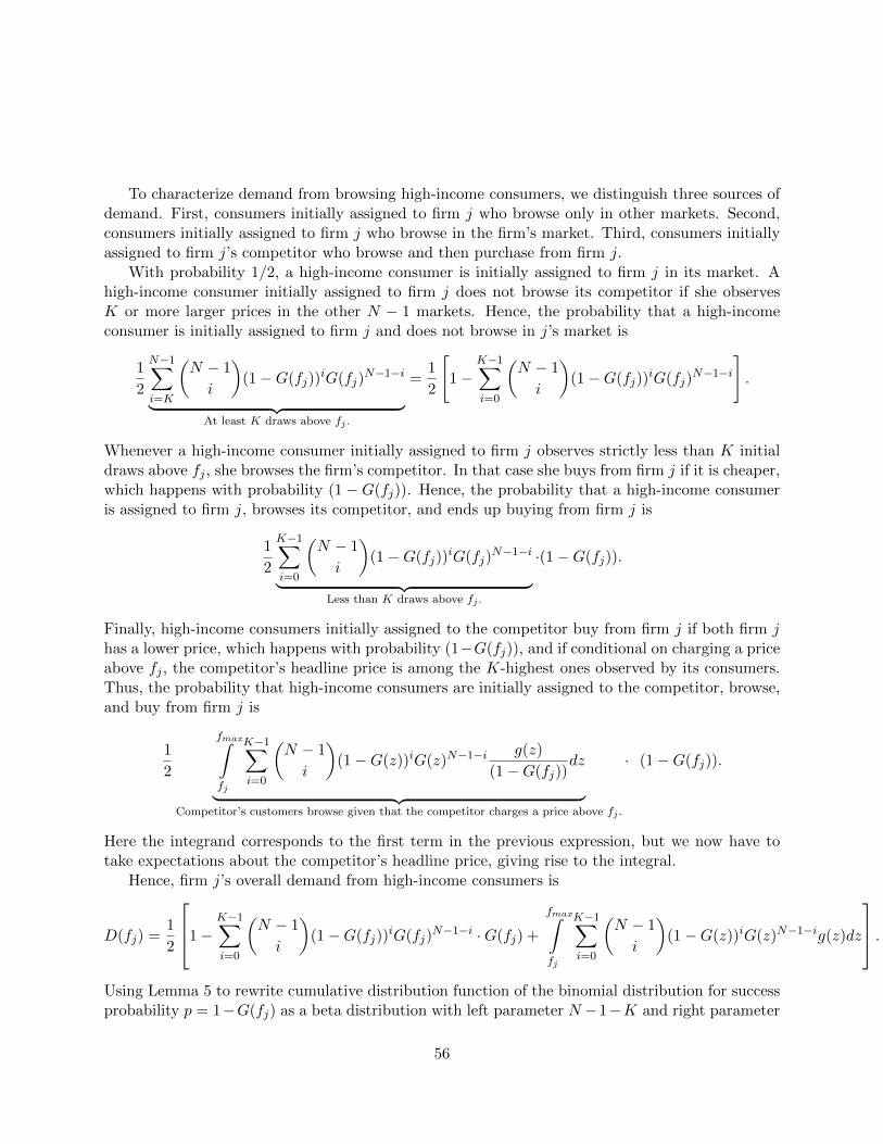
To characterize demand from browsing high-income consumers, we distinguish three sources ofdemand. First, consumers initially assigned to firm j who browse only in other markets. Second,consumers initially assigned to firm j who browse in the firm’s market. Third, consumers initiallyassigned to firm j’s competitor who browse and then purchase from firm j.

With probability 1/2, a high-income consumer is initially assigned to firm j in its market. Ahigh-income consumer initially assigned to firm j does not browse its competitor if she observesK or more larger prices in the other N − 1 markets. Hence, the probability that a high-incomeconsumer is initially assigned to firm j and does not browse in j’s market is

1

2

N−1∑i=K

(N − 1

i

)(1−G(fj))

iG(fj)N−1−i

︸︷︷︸At least K draws above fj .

=1

2

[1−

K−1∑i=0

(N − 1

i

)(1−G(fj))

iG(fj)N−1−i

].

Whenever a high-income consumer initially assigned to firm j observes strictly less than K initialdraws above fj , she browses the firm’s competitor. In that case she buys from firm j if it is cheaper,which happens with probability (1−G(fj)). Hence, the probability that a high-income consumeris assigned to firm j, browses its competitor, and ends up buying from firm j is

1

2

K−1∑i=0

(N − 1

i

)(1−G(fj))

iG(fj)N−1−i

︸︷︷︸Less than K draws above fj .

·(1−G(fj)).

Finally, high-income consumers initially assigned to the competitor buy from firm j if both firm jhas a lower price, which happens with probability (1−G(fj)), and if conditional on charging a priceabove fj , the competitor’s headline price is among the K-highest ones observed by its consumers.Thus, the probability that high-income consumers are initially assigned to the competitor, browse,and buy from firm j is

1

2

fmax∫fj

K−1∑i=0

(N − 1

i

)(1−G(z))iG(z)N−1−i

g(z)

(1−G(fj))dz

︸︷︷︸Competitor’s customers browse given that the competitor charges a price above fj .

· (1−G(fj)).

Here the integrand corresponds to the first term in the previous expression, but we now have totake expectations about the competitor’s headline price, giving rise to the integral.

Hence, firm j’s overall demand from high-income consumers is

D(fj) =1

2

1−K−1∑i=0

(N − 1

i

)(1−G(fj))

iG(fj)N−1−i ·G(fj) +

fmax∫fj

K−1∑i=0

(N − 1

i

)(1−G(z))iG(z)N−1−ig(z)dz

.Using Lemma 5 to rewrite cumulative distribution function of the binomial distribution for successprobability p = 1−G(fj) as a beta distribution with left parameter N −1−K and right parameter

56

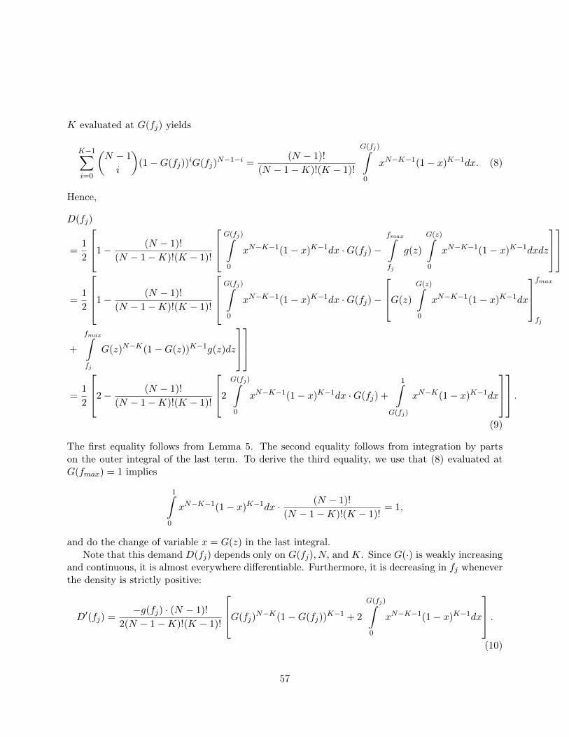
K evaluated at G(fj) yields

K−1∑i=0

(N − 1

i

)(1−G(fj))

iG(fj)N−1−i =

(N − 1)!

(N − 1−K)!(K − 1)!

G(fj)∫0

xN−K−1(1− x)K−1dx. (8)

Hence,

D(fj)

=1

2

1− (N − 1)!

(N − 1−K)!(K − 1)!

G(fj)∫0

xN−K−1(1− x)K−1dx ·G(fj)−fmax∫fj

g(z)

G(z)∫0

xN−K−1(1− x)K−1dxdz

=1

2

1− (N − 1)!

(N − 1−K)!(K − 1)!

G(fj)∫0

xN−K−1(1− x)K−1dx ·G(fj)−

G(z)

G(z)∫0

xN−K−1(1− x)K−1dx

fmax

fj

+

fmax∫fj

G(z)N−K(1−G(z))K−1g(z)dz

=1

2

2− (N − 1)!

(N − 1−K)!(K − 1)!

2

G(fj)∫0

xN−K−1(1− x)K−1dx ·G(fj) +

1∫G(fj)

xN−K(1− x)K−1dx

.

(9)

The first equality follows from Lemma 5. The second equality follows from integration by partson the outer integral of the last term. To derive the third equality, we use that (8) evaluated atG(fmax) = 1 implies

1∫0

xN−K−1(1− x)K−1dx · (N − 1)!

(N − 1−K)!(K − 1)!= 1,

and do the change of variable x = G(z) in the last integral.Note that this demand D(fj) depends only on G(fj), N, and K. Since G(·) is weakly increasing

and continuous, it is almost everywhere differentiable. Furthermore, it is decreasing in fj wheneverthe density is strictly positive:

D′(fj) =−g(fj) · (N − 1)!

2(N − 1−K)!(K − 1)!

G(fj)N−K(1−G(fj))

K−1 + 2

G(fj)∫0


.(10)

57

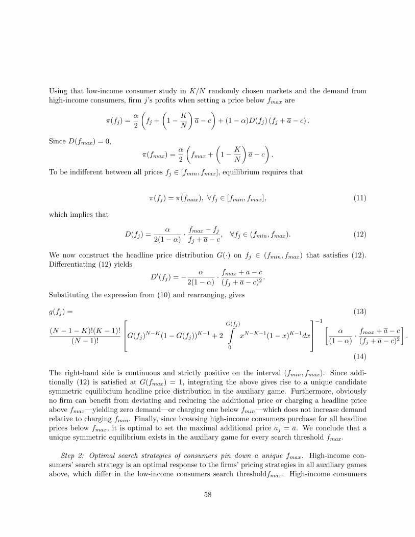
Using that low-income consumer study in K/N randomly chosen markets and the demand fromhigh-income consumers, firm j’s profits when setting a price below fmax are

π(fj) =α

2

(fj +

(1− K

N

)a− c

)+ (1− α)D(fj) (fj + a− c) .

Since D(fmax) = 0,

π(fmax) =α

2

(fmax +

(1− K

N

)a− c

).

To be indifferent between all prices fj ∈ [fmin, fmax], equilibrium requires that

π(fj) = π(fmax), ∀fj ∈ [fmin, fmax], (11)

which implies that

D(fj) =α

2(1− α)· fmax − fjfj + a− c

, ∀fj ∈ (fmin, fmax). (12)

We now construct the headline price distribution G(·) on fj ∈ (fmin, fmax) that satisfies (12).Differentiating (12) yields

D′(fj) = − α

2(1− α)· fmax + a− c

(fj + a− c)2.

Substituting the expression from (10) and rearranging, gives

g(fj) = (13)

(N − 1−K)!(K − 1)!

(N − 1)!

G(fj)N−K(1−G(fj))

K−1 + 2

G(fj)∫0


−1 [

α

(1− α)· fmax + a− c

(fj + a− c)2

].

(14)

The right-hand side is continuous and strictly positive on the interval (fmin, fmax). Since addi-tionally (12) is satisfied at G(fmax) = 1, integrating the above gives rise to a unique candidatesymmetric equilibrium headline price distribution in the auxiliary game. Furthermore, obviouslyno firm can benefit from deviating and reducing the additional price or charging a headline priceabove fmax—yielding zero demand—or charging one below fmin—which does not increase demandrelative to charging fmin. Finally, since browsing high-income consumers purchase for all headlineprices below fmax, it is optimal to set the maximal additional price aj = a. We conclude that aunique symmetric equilibrium exists in the auxiliary game for every search threshold fmax.

Step 2: Optimal search strategies of consumers pin down a unique fmax. High-income con-sumers’ search strategy is an optimal response to the firms’ pricing strategies in all auxiliary gamesabove, which differ in the low-income consumers search thresholdfmax. High-income consumers

58

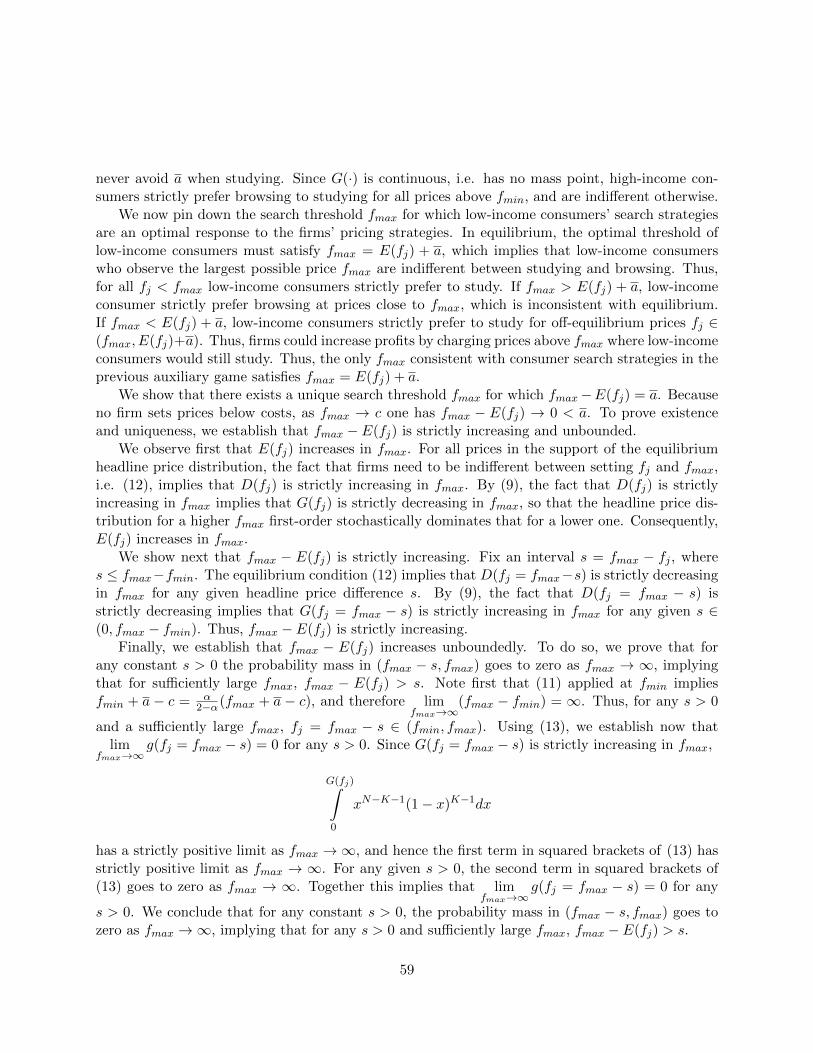
never avoid a when studying. Since G(·) is continuous, i.e. has no mass point, high-income con-sumers strictly prefer browsing to studying for all prices above fmin, and are indifferent otherwise.

We now pin down the search threshold fmax for which low-income consumers’ search strategiesare an optimal response to the firms’ pricing strategies. In equilibrium, the optimal threshold oflow-income consumers must satisfy fmax = E(fj) + a, which implies that low-income consumerswho observe the largest possible price fmax are indifferent between studying and browsing. Thus,for all fj < fmax low-income consumers strictly prefer to study. If fmax > E(fj) + a, low-incomeconsumer strictly prefer browsing at prices close to fmax, which is inconsistent with equilibrium.If fmax < E(fj) + a, low-income consumers strictly prefer to study for off-equilibrium prices fj ∈(fmax, E(fj)+a). Thus, firms could increase profits by charging prices above fmax where low-incomeconsumers would still study. Thus, the only fmax consistent with consumer search strategies in theprevious auxiliary game satisfies fmax = E(fj) + a.

We show that there exists a unique search threshold fmax for which fmax−E(fj) = a. Becauseno firm sets prices below costs, as fmax → c one has fmax − E(fj) → 0 < a. To prove existenceand uniqueness, we establish that fmax − E(fj) is strictly increasing and unbounded.

We observe first that E(fj) increases in fmax. For all prices in the support of the equilibriumheadline price distribution, the fact that firms need to be indifferent between setting fj and fmax,i.e. (12), implies that D(fj) is strictly increasing in fmax. By (9), the fact that D(fj) is strictlyincreasing in fmax implies that G(fj) is strictly decreasing in fmax, so that the headline price dis-tribution for a higher fmax first-order stochastically dominates that for a lower one. Consequently,E(fj) increases in fmax.

We show next that fmax − E(fj) is strictly increasing. Fix an interval s = fmax − fj , wheres ≤ fmax−fmin. The equilibrium condition (12) implies that D(fj = fmax−s) is strictly decreasingin fmax for any given headline price difference s. By (9), the fact that D(fj = fmax − s) isstrictly decreasing implies that G(fj = fmax − s) is strictly increasing in fmax for any given s ∈(0, fmax − fmin). Thus, fmax − E(fj) is strictly increasing.

Finally, we establish that fmax − E(fj) increases unboundedly. To do so, we prove that forany constant s > 0 the probability mass in (fmax − s, fmax) goes to zero as fmax → ∞, implyingthat for sufficiently large fmax, fmax − E(fj) > s. Note first that (11) applied at fmin impliesfmin + a − c = α

2−α(fmax + a − c), and therefore limfmax→∞

(fmax − fmin) = ∞. Thus, for any s > 0

and a sufficiently large fmax, fj = fmax − s ∈ (fmin, fmax). Using (13), we establish now thatlim

fmax→∞g(fj = fmax − s) = 0 for any s > 0. Since G(fj = fmax − s) is strictly increasing in fmax,

G(fj)∫0


has a strictly positive limit as fmax →∞, and hence the first term in squared brackets of (13) hasstrictly positive limit as fmax → ∞. For any given s > 0, the second term in squared brackets of(13) goes to zero as fmax → ∞. Together this implies that lim

fmax→∞g(fj = fmax − s) = 0 for any

s > 0. We conclude that for any constant s > 0, the probability mass in (fmax − s, fmax) goes tozero as fmax →∞, implying that for any s > 0 and sufficiently large fmax, fmax − E(fj) > s.

59

Step 3: Comparative Statics. Let Γ ≡ fmax − E(fj)− a = 0. Note that

E(fj) = fmin +

fmax∫fmin

(1−G(fj))df.

Since (12) is continuous in G(fj), c, a, α, fmin, and fmax, and since Γ is continuous in fmax, fmin, a,and G(fj), the derivative of fmax, fmin, and G(fj) with respect to any of these variables exists.

Consequently, for any parameter x that influences G(·), one has∂E(fj)∂x = −

fmax∫fmin

∂G(fj)∂x df . Thus, if

G(fj) decreases (increases) in x for all fj , the expected value increases (decreases) in x.Using the implicit-function theorem on Γ, we see that

∂fmax∂α

= −[

∂Γ

∂fmax

]−1 [∂Γ

∂α

]=

[1− ∂E(f)

∂fmax

]−1 [∂E(f)

∂α

]> 0.

We have shown above that E(fj) and fmax−E(fj) are increasing in fmax, so that ∂E(fj)/∂fmax ∈(0, 1), and since G(fj) decreases in α for all fj , we know that ∂E(fj)/∂α > 0, and therefore∂fmax∂α > 0. Consequently, profits and expected payments increase in the share of low-income

consumers.Similarly, we obtain that

∂E(fj)∂c > 0 and

∂E(fj)∂a < 0.

Proof of Proposition 8. Part 1: If J ≤ N − K, then there is an equilibrium in which thedistribution of firms’ prices is the same as in Proposition 7, and there is no equilibrium in whichall firms charge the additional price a along with the zero-profit headline price. We first establishthe existence of the equilibrium that mimics the headline price distribution of Proposition 7. Todo so, we solve for the symmetric equilibrium price distributions supposing that (i) high-incomeconsumers browse; (ii) if all observed headline prices are below the threshold fmax we characterizedin the proof of Proposition 7, low-income consumers study with equal probability in K of theN − J unregulated markets and avoid the additional price in the J regulated markets withoutstudying; if one price is above fmax, low-income consumers browse in the corresponding marketand study in K − 1 unregulated markets in which the headline price is below fmax, selecting eachthese markets with equal probability. (As before, we do not specify search behavior for the casethat more than two headline prices above fmax are observed by a low-income consumer becausethis requires simultaneous deviations by two or more firms and, thus, is irrelevant for equilibriumincentives.)

Given that high-income consumers browse and pay for the additional price in all markets, itis strictly optimal for firms to charge ai = a when choosing a headline price below fmax. Whencharging a headline price above fmax, a firm makes no sales and hence such a headline price issuboptimal. In a regulated market, for any headline price below fmax the firm sells to all low-income consumers initially assigned to it, and—because high-income consumers browse the highestK prices across all markets—the demand from high-income consumers is the same D(·) we solvedfor in the proof of Proposition 7. Hence, for headline prices below fmax profits are

π(fj) =α

2(fj − c) + (1− α)D(fj) (fj + a− c) .

60

Rewriting the equilibrium condition that π(fj) = π(fmax) for all headline prices in (fmin, fmax)shows that for all equilibrium headline prices

D(fj) =α

2(1− α)· fmax − fjfj + a− c

, ∀fj ∈ (fmin, fmax), (15)

which is identical to (12) in the proof of Proposition 7. Hence, since equilibrium requires the exactsame demand from browsing high-income consumers, it is solved by the same equilibrium headlineprice distribution G(·). Since the headline price does not affect low-income consumers’ studyingdecisions, the exact same steps as above demonstrate that G(·) is also the equilibrium headlineprice distribution in the unregulated markets.

To establish that G(·) still gives rise to an equilibrium, we still need to verify that the consumersearch behavior remains optimal. This is immediate for high-income consumers who do not wantto avoid the additional price. Now consider a low-income consumer for whom the highest observedheadline price is fmax. We argue that she is indifferent between browsing in the correspondingmarket and studying in an unregulated markets. This implies that she finds studying optimal if allprices are below fmax and browsing optimal when one headline price is above fmax.

When observing a maximal headline price of fmax, browsing in the corresponding market leadsto an expected headline-price saving of fmax−E(f) independent of whether the market is regulatedor unregulated. But in case the low-income consumer browses in this market, she can only studyin K − 1 unregulated markets, implying that she incurs the additional price in one extra marketleading to a higher expenditure on additional prices of a. Since for the equilibrium headline pricedistribution fmax − E(f) = a, she is exactly indifferent between browsing and studying. Weconclude that low-income consumer search behavior is optimal, and hence that we have specified asymmetric price distribution.

Next, we show that if J ≤ N − K, there exists no equilibrium in which all firms charge theadditional price a along with the zero-profit headline price. Suppose otherwise. Let f denote thezero-profit headline price. Consider the case in which firm i sets a headline price fi and all rivalsset f . In case fi < f + a, it is strictly optimal for low-income consumers to study. Hence, whenall firms set f low-income consumers study and therefore do not pay the additional price in allmarkets. As a result, the zero-profit headline price f > c − a. If firm i deviates and charges aheadline price fi ∈ (c, f + a) it earns strictly positive profits from any consumer it attracts, and itkeeps its initially assigned low-income consumers, a contradiction.

Part 2: If J > N−K, then there is an equilibrium in which all firms charge the additional pricea along with the zero-profit headline price, and there is no equilibrium in which the distributionof firms’ prices is the same as in Proposition 7. We prove the existence of such a zero-profitequilibrium. Let f = c − (1 − α)a be zero-profit headline price. Consider the following consumersearch strategy. In case a consumer observes a headline price weakly below f in all markets initially,they browse each of the N market with probability [K − (N − J)]/N , and then study in the N − Junregulated markets a lowest-price firm. In case consumers observe one headline price fi > f andall others equal to f , both types of consumers browse in i’s market with probability one, browsein all other markets with probability [K − (N − J) − 1]/(N − 1), and then study in the N − Junregulated markets a lowest-price firm.

61

Consider a firm i. Setting ai = a does not decrease demand and increases the revenue from con-sumers, strictly so for high-income consumers. Deviating to a headline price fi > f is unprofitableas it results in zero demand, and a headline price fi < f attracts the same proportion of high- andlow-income consumers than the firm attracts in equilibrium, and hence leads to negative profits.We conclude that the firms have no incentive to deviate.

It remains to show that the consumers’ search strategy is optimal. Consider low-income con-sumers first. Given search strategy, the avoid paying the additional price in all markets. Givenall initially observed prices are weakly below f , the search strategy ensures that they avoid payingthe additional price in all markets and buy at the cheapest headline price they have seen in eachmarket. Furthermore, any additional studying or browsing does not save money as in equilibriumfirms set fi = f . If one firm sets a price above f , low-income consumers can save money by initiallybrowsing in that market and thereafter studying in all unregulated markets a cheapest-priced firm.Furthermore, any additional browsing or studying would not save an money, which implies thattheir search strategy is optimal. High-income consumers cannot save any additional money frombrowsing or studying as long as at most one price they initially observe is above f , and hence theirsearch strategy is optimal.

We are left to show that there is no equilibrium in which the distribution of firms’ prices is thesame as in Proposition 7. Suppose otherwise. Since fmax = E(f) + a, low-income consumers studywith probability one in all unregulated markets when observing initial headline prices below fmaxin all markets. Furthermore, since they observe fmin with probability zero and all firms use thesame headline price distribution, they must browse in the K− (N −J) markets in which the initialheadline price is highest. When observing initial headline price above fmin, high-income consumersstrictly prefer browsing and hence must do so. Consider fi = max{fmin, c}. Since fmax > c,fi < fmax. Because any firm setting fi, a attracts high-income consumers with positive probabilityand cannot loose money from low-income consumers, it earns strictly positive profits. Denote theseprofits by π. As fi → fmax, firm i’s probability of being the highest-price firm goes to one, andtherefore its profits to zero. This contradicts that it must earn at least π for almost all prices inthe support.

Proof of Proposition 9. It follows from Lemmas 3 and 4 that firms 1 and 2 play symmetricstrategies in equilibrium, and that high-value consumers browse while low-value consumers studywith probability one. Furthermore, the symmetric equilibrium headline price distribution of firms1 and 2 has no mass point. Let fmax and fmin be the supremum and infimum of the incumbentfirms’ headline price distribution.

We proceed in four steps. First, we pin down equilibrium profits and price distributions. Second,we continue by showing that fmax ≤ min{(1/2)E(f) + (1/2)E3(f3) + a, vL}. Third, we establishthat if fmax < vL, then fmax is strictly increasing in α. Fourth, we show that there exists a uniqueα∗ ∈ (0, 1) such that fmax = vL if and only if α ≥ α∗.

Step (i): Equilibrium profits and price distributions. We show first that firm 3 has no masspoint on its support. Suppose otherwise that firm 3 has a mass point at some price f3. Then firms1 and 2 must set headline prices in an interval (f3, f3 + η) for some η > 0, since otherwise firm 3would earn zero profits at the mass point, contradicting Lemma 2. Additionally the incumbents

62

must set headline prices in an interval (f3, f3 + η) for any η > 0, since otherwise firm 3 couldincrease profits by shifting probability mass from f3 to a marginally larger headline price. But thenan incumbent can increase demand by shifting probability mass from (f3, f3+η) to f3−η/2 for anyη > 0. This does not affect demand from studying low-value consumers, but discretely increasesdemand from browsing high-value consumers who would otherwise switch to firm 3 more often.Since for a sufficiently small η, the loss in margins is negligible, this deviation strictly increasesprofits, contradicting that firm 3 has a mass point on its support. We conclude that firm 3 has nomass point on its support.

We continue by showing that G1(·) and G2(·) have a connected support. Suppose otherwisethat there exists an interval (f , f) ⊂ (fmin, fmax) such that G1(f) = G2(f) = const. ∈ (0, 1) forall f ∈ (f , f), and take (f , f) to be the largest such interval such that incumbent firms set pricesin any interval (f − η, f) and (f , f + η) for any η > 0. Then the headline price of firm 3 eitherhas no probability mass in (f , f), or has probability mass only on f . But then an incumbent firmcan strictly increase profits from consumers who buy by shifting probability mass from (f − η, f)to f − η/2 for any η > 0. Since by Lemma 4, the headline price distributions of firms 1 and 2 haveno mass point, the loss in demand goes to zero as η gets arbitrarily small. Thus, for a sufficientlysmall η > 0, this deviation strictly increases profits, contradicting that firms 1 and 2 do not haveconnected support. We conclude that firms 1 and 2 have connected support.

Denoting Gi(·) the headline price distribution of firm i, we use the fact that no firm has a masspoint in the headline price distribution and that ai = a by Lemma 1 to write the profits of firm 1as

1

2α(f1−c)+

1

2(1−α)

[1

2(1−G2(f1)) +

1

2(1−G3(f1))

](f1+a−c)+

1

2

1− α2

(1−G2(f1))(f1+a−c).

The first term are profits from low-value consumers. The second term are profits from high-valueconsumers who initially observe headline prices of firm 1. The term in squared brackets capturesthat with equal probability, these consumers compare prices with firm 2 or firm 3. The third termcaptures profits from poaching high-value consumers that initially observe f2. Exchanging indices1 and 2 leads to the profits of firm 2. Rearranging terms simplifies the expression to

1

2α(f1 − c) +

1

2(1− α)

[(1−G2(f1)) +

1

2(1−G3(f1))

](f1 + a− c). (16)

Low-value consumers are a profit base for firms 1 and 2 and these firms earn at least (1/2)α(fmax−c) by charging fmax. They must earn at least these profits for almost all prices in the support,implying that total prices fi+a are almost surely strictly larger than c. Hence fmin+a > c. There-fore the entrant charges the tuple (fmin, a) and thereby profitably attracts all browsing high-valueconsumers that see its headline price with probability one. Furthermore, the highest price in thesupport of firm 3’s headline price distribution, denoted f3, satisfies f3 < fmax for firm 3 to earnpositive profits since there is no mass point at fmax.

Therefore, firms 1 and 2 earn profits (1/2)α(fmax − c) when setting the largest price fmax.Hence, for almost all headline prices firms 1 and 2 must earn these profits. Since there is no masspoint at fmin, firms earn α/2(fmin − c) + 3/4(1 − α)(fmin + a − c) when charging fmin. Thus,

63

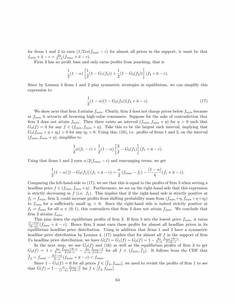
for firms 1 and 2 to earn (1/2)α(fmax − c) for almost all prices in the support, it must be thatfmin + a− c = 2α

3−α(fmax + a− c).Firm 3 has no profit base and only earns profits from poaching, that is

1

2(1− α)

[1

2(1−G1(f3)) +

1

2(1−G2(f3))

](f3 + a− c).

Since by Lemma 4 firms 1 and 2 play symmetric strategies in equilibrium, we can simplify thisexpression to

1

2(1− α)(1−G2(f3))(f3 + a− c). (17)

We show next that firm 3 attains fmin. Clearly, firm 3 does not charge prices below fmin becauseat fmin it attracts all browsing high-value consumers. Suppose for the sake of contradiction thatfirm 3 does not attain fmin. Then there exists an interval (fmin, fmin + η) for η > 0 such thatG3(f) = 0 for any f ∈ (fmin, fmin + η). Take this to be the largest such interval, implying thatG3(fmin + η + η2) > 0 for any η2 > 0. Using this, (16), i.e. profits of firms 1 and 2, on the interval(fmin, fmin + η), simplifies to

1

2α(f1 − c) +

1

2(1− α)

[3

2−G2(f1)

](f1 + a− c).

Using that firms 1 and 2 earn α/2(fmax − c) and rearranging terms, we get

1

2(1− α) [1−G2(f1)] (f1 + a− c) =

α

2(fmax − f1)−

(1− α)

4(f1 + a− c).

Comparing the left-hand-side to (17), we see that this is equal to the profits of firm 3 when setting aheadline price f ∈ (fmin, fmin+η) . Furthermore, we see on the right-hand side that this expressionis strictly decreasing in f (i.e. f1). This implies that if the right-hand side is strictly positive atf1 = fmin, firm 3, could increase profits from shifting probability mass from (fmin+η, fmin+η+η2)to fmin for a sufficiently small η2 > 0. Since the right-hand side is indeed strictly positive atf1 = fmin for all α ∈ (0, 1), this contradicts that firm 3 does not attain fmin. We conclude thatfirm 3 attains fmin.

This pins down the equilibrium profits of firm 3. If firm 3 sets the lowest price fmin, it earns(1−α)α(3−α) (fmax + a − c). Hence firm 3 must earn these profits for almost all headline prices in its

equilibrium headline price distribution. Using in addition that firms 1 and 2 have a symmetricheadline price distribution by Lemma 4, (17) implies that for almost all f in the support of firm3’s headline price distribution, we have G(f) = G1(f) = G2(f) = 1− 2α

3−αfmax+a−cf+a−c .

In the next step, we use G2(f) and (16) as well as the equilibrium profits of firm 3 to getG3(f) = 1 + 4α

3−αfmax+a−cf+a−c − 2α

1−αfmax−ff+a−c for all f ∈ (fmin, f3). It follows from the CDF that

f3 = fmax − 2(1−α)3−α (fmax + a− c) < fmax.

Since 1 −G3(f) = 0 for all prices f ∈ [f3, fmax], we need to revisit the profits of firm 1 to seethat G(f) = 1− α

(1−α)fmax−ff+a−c for f ∈ [f3, fmax].

64

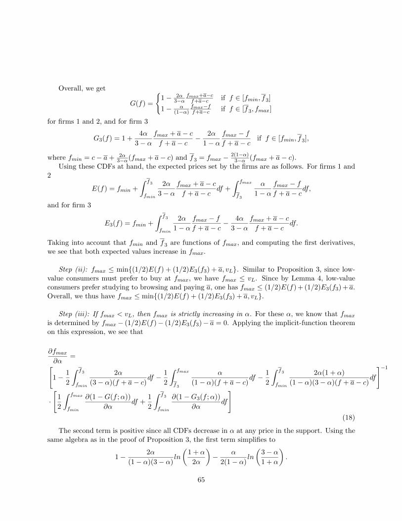
Overall, we get

G(f) =

{1− 2α

3−αfmax+a−cf+a−c if f ∈ [fmin, f3]

1− α(1−α)

fmax−ff+a−c if f ∈ [f3, fmax]

for firms 1 and 2, and for firm 3

G3(f) = 1 +4α

3− αfmax + a− cf + a− c

− 2α

1− αfmax − ff + a− c

if f ∈ [fmin, f3],

where fmin = c− a+ 2α3−α(fmax + a− c) and f3 = fmax − 2(1−α)

3−α (fmax + a− c).Using these CDFs at hand, the expected prices set by the firms are as follows. For firms 1 and

2

E(f) = fmin +

∫ f3

fmin

2α


df +

∫ fmax

f3

α


df,

and for firm 3

E3(f) = fmin +

∫ f3

fmin

2α


− 4α


df.

Taking into account that fmin and f3 are functions of fmax, and computing the first derivatives,we see that both expected values increase in fmax.

Step (ii): fmax ≤ min{(1/2)E(f) + (1/2)E3(f3) + a, vL}. Similar to Proposition 3, since low-value consumers must prefer to buy at fmax, we have fmax ≤ vL. Since by Lemma 4, low-valueconsumers prefer studying to browsing and paying a, one has fmax ≤ (1/2)E(f) + (1/2)E3(f3) + a.Overall, we thus have fmax ≤ min{(1/2)E(f) + (1/2)E3(f3) + a, vL}.

Step (iii): If fmax < vL, then fmax is strictly increasing in α. For these α, we know that fmaxis determined by fmax− (1/2)E(f)− (1/2)E3(f3)− a = 0. Applying the implicit-function theoremon this expression, we see that

∂fmax∂α

=[1− 1

2

∫ f3

fmin

2α

(3− α)(f + a− c)df − 1

2

∫ fmax

f3

α

(1− α)(f + a− c)df − 1

2

∫ f3

fmin

2α(1 + α)

(1− α)(3− α)(f + a− c)df

]−1

·

[1

2

∫ fmax

fmin

∂(1−G(f ;α))

∂αdf +

1

2

∫ f3

fmin

∂(1−G3(f ;α))

∂αdf

](18)

The second term is positive since all CDFs decrease in α at any price in the support. Using thesame algebra as in the proof of Proposition 3, the first term simplifies to

1− 2α

(1− α)(3− α)ln

(1 + α

2α

)− α

2(1− α)ln

(3− α1 + α

).

65

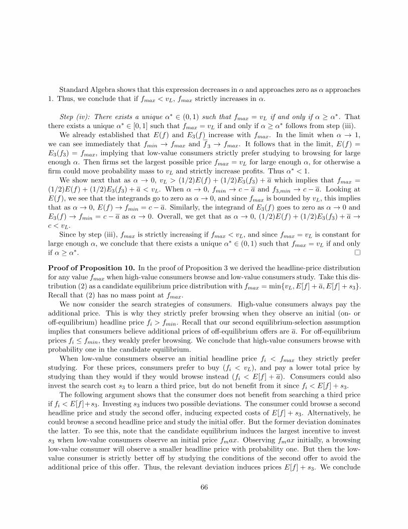
Standard Algebra shows that this expression decreases in α and approaches zero as α approaches1. Thus, we conclude that if fmax < vL, fmax strictly increases in α.

Step (iv): There exists a unique α∗ ∈ (0, 1) such that fmax = vL if and only if α ≥ α∗. Thatthere exists a unique α∗ ∈ [0, 1] such that fmax = vL if and only if α ≥ α∗ follows from step (iii).

We already established that E(f) and E3(f) increase with fmax. In the limit when α → 1,we can see immediately that fmin → fmax and f3 → fmax. It follows that in the limit, E(f) =E3(f3) = fmax, implying that low-value consumers strictly prefer studying to browsing for largeenough α. Then firms set the largest possible price fmax = vL for large enough α, for otherwise afirm could move probability mass to vL and strictly increase profits. Thus α∗ < 1.

We show next that as α → 0, vL > (1/2)E(f) + (1/2)E3(f3) + a which implies that fmax =(1/2)E(f) + (1/2)E3(f3) + a < vL. When α → 0, fmin → c − a and f3,min → c − a. Looking atE(f), we see that the integrands go to zero as α→ 0, and since fmax is bounded by vL, this impliesthat as α→ 0, E(f)→ fmin = c− a. Similarly, the integrand of E3(f) goes to zero as α→ 0 andE3(f) → fmin = c − a as α → 0. Overall, we get that as α → 0, (1/2)E(f) + (1/2)E3(f3) + a →c < vL.

Since by step (iii), fmax is strictly increasing if fmax < vL, and since fmax = vL is constant forlarge enough α, we conclude that there exists a unique α∗ ∈ (0, 1) such that fmax = vL if and onlyif α ≥ α∗.

Proof of Proposition 10. In the proof of Proposition 3 we derived the headline-price distributionfor any value fmax when high-value consumers browse and low-value consumers study. Take this dis-tribution (2) as a candidate equilibrium price distribution with fmax = min{vL, E[f ] + a,E[f ] + s3}.Recall that (2) has no mass point at fmax.

We now consider the search strategies of consumers. High-value consumers always pay theadditional price. This is why they strictly prefer browsing when they observe an initial (on- oroff-equilibrium) headline price fi > fmin. Recall that our second equilibrium-selection assumptionimplies that consumers believe additional prices of off-equilibrium offers are a. For off-equilibriumprices fi ≤ fmin, they weakly prefer browsing. We conclude that high-value consumers browse withprobability one in the candidate equilibrium.

When low-value consumers observe an initial headline price fi < fmax they strictly preferstudying. For these prices, consumers prefer to buy (fi < vL), and pay a lower total price bystudying than they would if they would browse instead (fi < E[f ] + a). Consumers could alsoinvest the search cost s3 to learn a third price, but do not benefit from it since fi < E[f ] + s3.

The following argument shows that the consumer does not benefit from searching a third priceif fi < E[f ]+s3. Investing s3 induces two possible deviations. The consumer could browse a secondheadline price and study the second offer, inducing expected costs of E[f ] + s3. Alternatively, hecould browse a second headline price and study the initial offer. But the former deviation dominatesthe latter. To see this, note that the candidate equilibrium induces the largest incentive to invests3 when low-value consumers observe an initial price fmax. Observing fmax initially, a browsinglow-value consumer will observe a smaller headline price with probability one. But then the low-value consumer is strictly better off by studying the conditions of the second offer to avoid theadditional price of this offer. Thus, the relevant deviation induces prices E[f ] + s3. We conclude

66

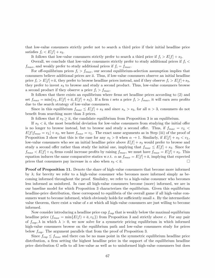
that low-value consumers strictly prefer not to search a third price if their initial headline pricesatisfies fi < E[f ] + s3.

It follows that low-value consumers strictly prefer to search a third price if fi > E[f ] + s3.Overall, we conclude that low-value consumers strictly prefer to study additional prices if fi <

fmax, and weakly prefer to study additional prices if fi = fmax.For off-equilibrium prices fi > fmax, our second equilibrium-selection assumption implies that

consumers believe additional prices are a. Thus, if low-value consumers observe an initial headlineprice fi > E[f ]+a, they prefer to browse headline prices instead, and if they observe fi > E[f ]+s3,they prefer to invest s3 to browse and study a second product. Thus, low-value consumers browsea second product if they observe a price fi > fmax.

It follows that there exists an equilibrium where firms set headline prices according to (2) andset fmax = min{vL, E[f ] + a,E[f ] + s3}. If a firm i sets a price fi > fmax, it will earn zero profitsdue to the search strategy of low-value consumers.

Since in this equilibrium fmax ≤ E[f ] + s3 and since sn > s3, for all n > 3, consumers do notbenefit from searching more than 3 prices.

It follows that if s3 ≥ a, the candidate equilibrium from Proposition 3 is an equilibrium.If s3 < a, the most beneficial deviation for low-value consumers from studying the initial offer

is no longer to browse instead, but to browse and study a second offer. Thus, if fmax = vL <E[f |fmax = vL] + s3, we have fmax = vL. The exact same arguments as in Step (iii) of the proof ofProposition 3 show that this is the case for any s3 > 0 when α → 1. Similarly, if E[f ] + s3 < vL,low-value consumers who see an initial headline price above E[f ] + s3 would prefer to browse andstudy a second offer rather than study the initial one, implying that fmax ≤ E[f ] + s3. Since forfmax < E[f ] + s3 firms could increase profits by raising fmax, we must have fmax = E[f ] + s3. Thisequation induces the same comparative statics w.r.t. α as fmax = E[f ] +a, implying that expectedprices that consumers pay increase in α also when s3 < a.

Proof of Proposition 11. Denote the share of high-value consumers that become more informedby λ; for brevity we refer to a high-value consumer who becomes more informed simply as be-coming informed throughout the proof. Similalry, we refer to a high-value consumer who becomesless informed as uninfored. In case all high-value consumers become (more) informed, we are inour baseline model for which Proposition 3 characterizes the equilibrium. Given this equilibriumheadline-price distribution, these correspond to equilibria of the overall game if all high-value con-sumers want to become informed, which obviously holds for sufficiently small s. By the intermediatevalue theorem, there exist a value of s at which all high-value consumers are just willing to becomeinformed.

Now consider introducing a headline price cap fcap that is weakly below the maximal equilibriumheadline price (fmax = min{E(f) + a, vL}) from Proposition 3 and strictly above c. For any pairof fcap, λ in which λ > 0, we now solve for a symmetric pricing equilibrium in which informedhigh-value consumers browse on the equilibrium path and low-value consumers study for pricesbelow fcap. The argument parallels that from the proof of Proposition 3.

Since fcap ≤ fmax and there can be no mass point in the symmetric equilibrium headline pricedistribution, a firm setting the highest headline price in the support of the equilibrium headlineprice distribution G sells to all low-value as well as to uninformed high-value consumers but does

67

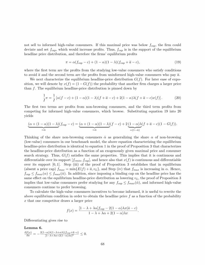
not sell to informed high-value consumers. If this maximal price was below fcap, the firm coulddeviate and set fcap, which would increase profits. Thus, fcap is in the support of the equilibriumheadline price distribution, and therefore the firms’ equilibrium profits

π = α(fcap − c) + (1− α)(1− λ)(fcap + a− c), (19)

where the first term are the profits from the studying low-value consumers who satisfy conditionsto avoid a and the second term are the profits from uninformed high-value consumers who pay a.

We next characterize the equilibrium headline-price distribution G(f). For later ease of expo-sition, we will denote by x(f) = (1−G(f)) the probability that another firm charges a larger pricethan f . The equilibrium headline-price distribution is pinned down by

1

Iπ =

1

I[α(f − c) + (1− α)(1− λ)(f + a− c) + 2(1− α)λ(f + a− c)x(f)] . (20)

The first two terms are profits from non-browsing consumers, and the third term profits fromcompeting for informed high-value consumers, which browse. Substituting equation 19 into 20yields

(α+ (1− α)(1− λ)︸︷︷︸=α

(fcap − c) = (α+ (1− α)(1− λ)︸︷︷︸=α

(f − c) + 2 (1− α)λ︸︷︷︸=(1−α)

(f + a− c)(1−G(f)).

Thinking of the share non-browsing consumers α as generalizing the share α of non-browsing(low-value) consumers in our benchmark model, the above equation characterizing the equilibriumheadline-price distribution is identical to equation 1 in the proof of Proposition 3 that characterizesthe headline-price distribution as a function of an exogenously given maximal price and consumersearch strategy. Thus, G(f) satisfies the same properties. This implies that it is continuous anddifferentiable over its support [fcmin, fcap], and hence also that x(f) is continuous and differentiableover its support [0, 1]. Step (iii) of the proof of Proposition 3 establishes that in equilibrium(absent a price cap) fmax = min{E(f) + a, vL}, and Step (iv) that fmax is increasing in α. Hence,fcap ≤ fmax(α) ≤ fmax(α). In addition, since imposing a binding cap on the headline price has thesame effect on the equilibrium headline-price distribution as lowering vL, the proof of Proposition 3implies that low-value consumers prefer studying for any fcap ≤ fmax(α), and informed high-valueconsumers continue to prefer browsing.

To calculate the high-value consumers incentives to become informed, it is useful to rewrite theabove equilibrium condition in order to obtain the headline price f as a function of the probabilityx that one competitor draws a larger price

f(x) =[1− λ+ λα]fcap − 2(1− α)λx(a− c)

1− λ+ λα+ 2(1− α)λx.

Differentiating gives rise to

Lemma 6.∂f(x)∂x = −2(1−α)λ(1−λ+αλ)(fcap+a−c)

[1−λ+λα+2(1−α)λx]2 ≤ 0.

68

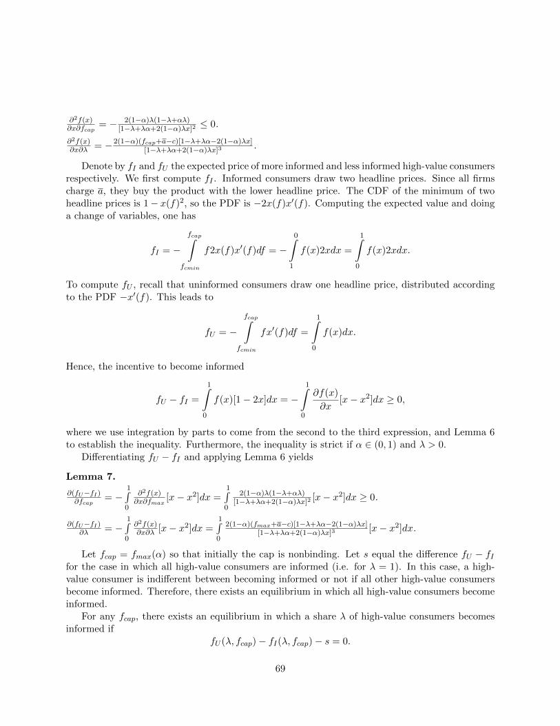
∂2f(x)∂x∂fcap

= − 2(1−α)λ(1−λ+αλ)[1−λ+λα+2(1−α)λx]2 ≤ 0.

∂2f(x)∂x∂λ = −2(1−α)(fcap+a−c)[1−λ+λα−2(1−α)λx]

[1−λ+λα+2(1−α)λx]3 .

Denote by fI and fU the expected price of more informed and less informed high-value consumersrespectively. We first compute fI . Informed consumers draw two headline prices. Since all firmscharge a, they buy the product with the lower headline price. The CDF of the minimum of twoheadline prices is 1− x(f)2, so the PDF is −2x(f)x′(f). Computing the expected value and doinga change of variables, one has

fI = −fcap∫

fcmin

f2x(f)x′(f)df = −0∫

1

f(x)2xdx =

1∫0

f(x)2xdx.

To compute fU , recall that uninformed consumers draw one headline price, distributed accordingto the PDF −x′(f). This leads to

fU = −fcap∫

fcmin

fx′(f)df =

1∫0

f(x)dx.

Hence, the incentive to become informed

fU − fI =

1∫0

f(x)[1− 2x]dx = −1∫

0

∂f(x)

∂x[x− x2]dx ≥ 0,

where we use integration by parts to come from the second to the third expression, and Lemma 6to establish the inequality. Furthermore, the inequality is strict if α ∈ (0, 1) and λ > 0.

Differentiating fU − fI and applying Lemma 6 yields

Lemma 7.

∂(fU−fI)∂fcap

= −1∫0

∂2f(x)∂x∂fmax

[x− x2]dx =1∫0

2(1−α)λ(1−λ+αλ)[1−λ+λα+2(1−α)λx]2 [x− x2]dx ≥ 0.

∂(fU−fI)∂λ = −

1∫0

∂2f(x)∂x∂λ [x− x2]dx =

1∫0

2(1−α)(fmax+a−c)[1−λ+λα−2(1−α)λx][1−λ+λα+2(1−α)λx]3 [x− x2]dx.

Let fcap = fmax(α) so that initially the cap is nonbinding. Let s equal the difference fU − fIfor the case in which all high-value consumers are informed (i.e. for λ = 1). In this case, a high-value consumer is indifferent between becoming informed or not if all other high-value consumersbecome informed. Therefore, there exists an equilibrium in which all high-value consumers becomeinformed.

For any fcap, there exists an equilibrium in which a share λ of high-value consumers becomesinformed if

fU (λ, fcap)− fI(λ, fcap)− s = 0.

69

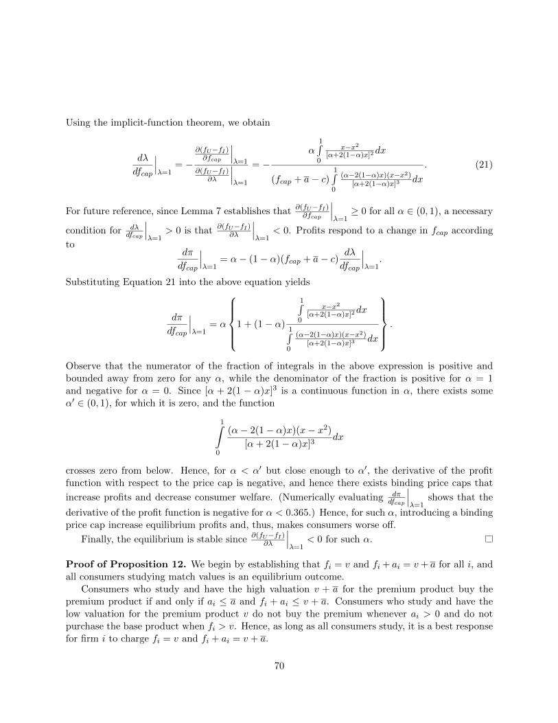
Using the implicit-function theorem, we obtain

dλ

dfcap

∣∣∣λ=1

= −∂(fU−fI)∂fcap

∣∣∣λ=1

∂(fU−fI)∂λ

∣∣∣λ=1

= −α

1∫0

x−x2[α+2(1−α)x]2dx

(fcap + a− c)1∫0

(α−2(1−α)x)(x−x2)[α+2(1−α)x]3 dx

. (21)

For future reference, since Lemma 7 establishes that ∂(fU−fI)∂fcap

∣∣∣λ=1≥ 0 for all α ∈ (0, 1), a necessary

condition for dλdfcap

∣∣∣λ=1

> 0 is that ∂(fU−fI)∂λ

∣∣∣λ=1

< 0. Profits respond to a change in fcap according

todπ

dfcap

∣∣∣λ=1

= α− (1− α)(fcap + a− c) dλ

dfcap

∣∣∣λ=1

.

Substituting Equation 21 into the above equation yields

dπ

dfcap

∣∣∣λ=1

= α

1 + (1− α)

1∫0

x−x2[α+2(1−α)x]2dx

1∫0

(α−2(1−α)x)(x−x2)[α+2(1−α)x]3 dx

.

Observe that the numerator of the fraction of integrals in the above expression is positive andbounded away from zero for any α, while the denominator of the fraction is positive for α = 1and negative for α = 0. Since [α + 2(1 − α)x]3 is a continuous function in α, there exists someα′ ∈ (0, 1), for which it is zero, and the function

1∫0

(α− 2(1− α)x)(x− x2)[α+ 2(1− α)x]3

dx

crosses zero from below. Hence, for α < α′ but close enough to α′, the derivative of the profitfunction with respect to the price cap is negative, and hence there exists binding price caps that

increase profits and decrease consumer welfare. (Numerically evaluating dπdfcap

∣∣∣λ=1

shows that the

derivative of the profit function is negative for α < 0.365.) Hence, for such α, introducing a bindingprice cap increase equilibrium profits and, thus, makes consumers worse off.

Finally, the equilibrium is stable since ∂(fU−fI)∂λ

∣∣∣λ=1

< 0 for such α.

Proof of Proposition 12. We begin by establishing that fi = v and fi + ai = v+ a for all i, andall consumers studying match values is an equilibrium outcome.

Consumers who study and have the high valuation v + a for the premium product buy thepremium product if and only if ai ≤ a and fi + ai ≤ v + a. Consumers who study and have thelow valuation for the premium product v do not buy the premium whenever ai > 0 and do notpurchase the base product when fi > v. Hence, as long as all consumers study, it is a best responsefor firm i to charge fi = v and fi + ai = v + a.

70

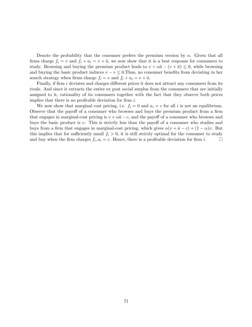
Denote the probability that the consumer prefers the premium version by α. Given that allfirms charge fi = v and fi + ai = v + a, we now show that it is a best response for consumers tostudy. Browsing and buying the premium product leads to v + αa − (v + a) ≤ 0, while browsingand buying the basic product induces v − v ≤ 0.Thus, no consumer benefits from deviating in hersearch strategy when firms charge fi = v and fi + ai = v + a.

Finally, if firm i deviates and charges different prices it does not attract any consumers from itsrivals. And since it extracts the entire ex post social surplus from the consumers that are initiallyassigned to it, rationality of its consumers together with the fact that they observe both pricesimplies that there is no profitable deviation for firm i.

We now show that marginal cost pricing, i.e. fi = 0 and ai = c for all i is not an equilibrium.Observe that the payoff of a consumer who browses and buys the premium product from a firmthat engages in marginal-cost pricing is v+ αa− c, and the payoff of a consumer who browses andbuys the basic product is v. This is strictly less than the payoff of a consumer who studies andbuys from a firm that engages in marginal-cost pricing, which gives α(v + a − c) + (1 − α)v. Butthis implies that for sufficiently small fi > 0, it is still strictly optimal for the consumer to studyand buy when the firm charges fi, ai = c. Hence, there is a profitable deviation for firm i.

71

Documents

Browsing versus Studying: A Pro-Market Case for Regulation · Browsing versus Studying: A Pro-Market Case for Regulation ... \study" both the headline and additional prices of one