Embed Size (px)
Citation preview
ELSEVIER European Journal of Operational Research 85 (1995) 192-204
EUROPEAN JOURNAL
OF OPERATIONAL RESEARCH
Theory and Methodology
Brownian motion approximations for tankage assessment and stock control
Roelant A.J.J. Nieboer 1, Rommert Dekker *
Koninklijke / Shell-Laboratorium, Amsterdam (Shell Research B.V..), P.O. Box 3003, 1003 AA Amsterdam, Netherlands
Received December 1991; revised July 1993
Abstract
This paper presents a model for refinery tankage assessment. Special characteristics covered are a hybrid demand process and a periodic-review target-stock policy for production control. The demand is assumed to be in two forms: as large parcels, collected at fixed intervals, and as many small parcels, modelled through a Brownian motion. Analytical approximations for the average stock level, the probability and expected volumes of overflow and stockout per period have been developed and compared with exact and simulation results. Using these approximations the problem of determining both the optimal tank capacity and the optimal target stock can be separated and solved rapidly on a PC. Finally, some sensitivity analyses to determine the most important model parameters have been carried out.
Keywords: Inventory; Production; Petroleum; Stochastic processes
1. Introduction
Tankage assessment is an important problem when constructing a new refinery tankfarm or rationaliz- ing an existing one, as almost all tanks have a dedicated purpose, which is costly to change. Moreover, existing tankage is often an important determinant of the amount of stocks a refinery has. Setting aside the fact that about 10% of the contents of a tank consists of unpumpables which cannot be used, refinery schedulers and traders tend to exploit existing tankage as much as possible without taking tankage or stock holding costs into account. A similar problem exists with respect to target stock setting: it is a common feeling among refinery schedulers that (apart from unpumpables) the ideal tank stock level is midway, because in that case one is most far away from both minimum and maximum level. However, the underlying assumption, viz. that the tank has the optimum size, is often violated and therefore better methods are needed for target stock setting.
* Corresponding author. Present address: Econometric Institute, Erasmus University Rotterdam, P.O. Box 1738, 3000 DR Rotterdam, Netherlands.
1 Present address: Shell Nederland Informatieverwerking B.V., P.O. Box 5835, 2280 HV Rijswijk, Netherlands.
0377-2217/95/$09.50 © 1995 Elsevier Science B.V. All rights reserved SSDI 0377-2217(93)E0356-3
R.A.J.J. Nieboer, R. Dekker / European Journal of Operational Research 85 (1995) 192-204 193
In this paper we analyse a basic model for tankage assessment. It is meant as a building block for larger and more complicated models as actual refinery operations are quite complex (see, e.g. Klingman et al., 1987, and Langeveld, 1989). The model was kept simple as to provide insight in the relationships between various logistic elements and moreover, to allow a nice analysis.
The model has three special characteristics. First, it deals with a single tank with finite capacity, taking both stockout and overflow into account. Next, it considers a hybrid demand process, in which both large parcels are collected (e.g. by an ocean going vessel) at fixed intervals and many small parcels are delivered almost continuously. The third characteristic concerns the use of a periodic-review target-stock policy. For quality reasons the production rate can only be changed after a period of fixed duration and its value is set such that the expected stock level at the end of the coming period equals a target value.
The model is analysed with respect to its long-term behaviour, that is, we calculate for a given tank capacity and target stock the long-term average stock level, the fraction of periods with smckout or overflow, and finally the average volumes of stockout and overflow. Brownian motion theory is used to analyse the model and we derive simple and complex approximations which are easy to evaluate. The approximations are compared with exact expressions for the Brownian motion and with simulations of a Poisson process. Next we show that the problem of optimising both the target stock and the tankage capacity can be separated in case of linear cost functions. Finally, we give some results on sensitivity analyses.
The model presented here has not been discussed elsewhere. Miltenburg and Silver (1984a,b) and Miltenburg (1987) also use a Brownian motion to approximate the pdf of the residual stock in periodic-review multiple-item inventory models. Shreve et al. (1984) cite a number of papers dealing with diffusion models in inventory/product ion control. These papers, however, are mainly concerned with determining the structure of optimal policies in far more simplified models. Odi and Karimi (1988) primarily consider intermediate tankage and determine the amount of tankage that would, with a given probability, decouple the supply process from the offtake process. They do not consider a controlled supply process, and their analysis is concerned more with worst cases than with the average behaviour.
The structure of this paper is as follows. In Section 2 we present the model, which is analysed in Section 3. In Section 4 simple and complex approximations, are derived. Using these the tank capacity and target stock level can easily be optimised, as is shown in Section 5. Section 6 deals with the numerical performance of the approximations and sensitivity analyses.
2. The model
Consider a tank with finite capacity K containing a (continuously divisible) product from which customers are supplied. A production unit feeds the tank continuously. After fixed periods of length t B the amount of stock in the tank is reviewed and the production rate can be adjusted. There are two types of demand. First, there is demand for small parcels by customers who arrive according to a Poisson process with arrival rate A, each collecting an amount of z. Next, there is demand for large parcels, which is planned in advance; in each period one large parcel of size L is collected exactly in the middle of the period. Demand which cannot be met from stock on hand is supplied later (complete backlogging); production which cannot be stored in the tank is stored in another, more expensive way and can be used to satisfy later demand. In fact, in this model the stock value can assume any value, if it is negative we speak of a stockout and if it is above K we speak of an overflow.
Summing over the two types of demand yields for the total expected demand per period E ( D ) = L +
h~-t B. The production rate is set according to a stationary target-stock rule, which works as follows. Let stg (0 < stg < K) denote the target-stock level, if s B is the observed stock level at the start of a period,
194 R.A.J.J. Nieboer, R. Dekker / European Journal o f Operational Research 85 (1995) 192-204
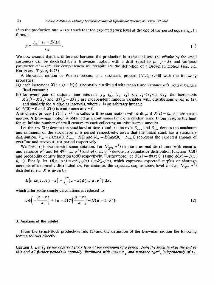
then the production rate 19 is set such that the expected stock level at the end of the period equals Stg. In formula,
Stg - s n + E ( D ) p = (1)
ta
We now assume that the difference between the production into the tank and the offtake by the small customers can be modelled by a Brownian motion with a drift equal to /x = p - Az and variance parameter 0.2= Are. For completeness we recapitulate the definition of a Brownian motion (see, e.g. Karlin and Taylor, 1975).
A Brownian motion or Wiener process is a stochastic process {X(t); t > 0} with the following properties: (a) each increment X( t + s) - X ( s ) is normally distributed with mean 0 and variance ITzt, with IT being a
fixed constant; (b) for every pair of disjoint time intervals [/1, t2], [t3, t4], say t I < t 2 < t 3 <t4, the increments
S ( t 4) - S ( t 3) and X ( t 2) - X ( t l ) are independent random variables with distributions given in (a), and similarly for n disjoint intervals, where n is an arbitrary integer;
(c) X(0) = 0 and X ( t ) is continuous at t = 0. A stochastic process {X(t); t > 0} is called a Brownian motion with drift /z if X ( t ) - tlz is a Brownian motion. A Brownian motion is obtained as a continuous limit of a random walk. In our case, as the limit for an infinite number of small customers each collecting an infinitesimal amount.
Let the r.v. S(t) denote the stocklevel at time t and let the r.v.'s Sm~ x and Smin denote the maximum and minimum of the stock level in a period respectively, given that the initial stock has a stationary distribution. Vov-'= E(max(0, Sm~ x - K ) ) and V~o := E(max(0, -Stain)) represent the expected amount of overflow and stockout in a period respectively.
We finish this section with some notation. Let N(/~, 0 -2) denote a normal distribution with mean /z and variance IT2 and let ~ ( . ; ~, 0.2) and ¢ ( . ; / z , 0.2) denote its cumulative distribution function (Cdf) and probability density function (pdf) respectively. Furthermore, let q0(x) := q~(x; 0, 1) and th(x) := ~b(x; 0, 1). Finally, let 12(/z, 0.2):= 0.~b(/z/iT)+/z~(/z/0.) , which expresses expected surplus or shortage amounts of a normally distributed r.v. For instance, the expected surplus above level z of an N(/z, 0.2) distributed r.v. X is given by
E [ m a x ( z , X ) - z ] = fz=(Z - x ) ~ b ( x ; ~z, IT2) dx ,
which after some simple calculations is reduced to
+ - z , IT2). IT
(2)
3. Analysis of the model
From the target-stock production rule (1) and the definition of the Brownian motion the following lemma follows directly.
Lemma 1. Let s B be the observed stock level at the beginning of a period. Then the stock level at the end of this and all further periods is normally distributed with mean stg and variance tB0. z, independently of s B.
R.A.J.J. Nieboer, R. Dekker / European Journal of Operational Research 85 (1995) 192-204 195
Lemma 1 implies that after one period, the stock level at the end of a period already assumes a stationary distribution, regardless of the initial stock level. To study the long-run behaviour of the stock process, we therefore need to consider one period only with a stationary distribution for the starting stock. In the sequel we will denote by t the time passed since the start of such a period.
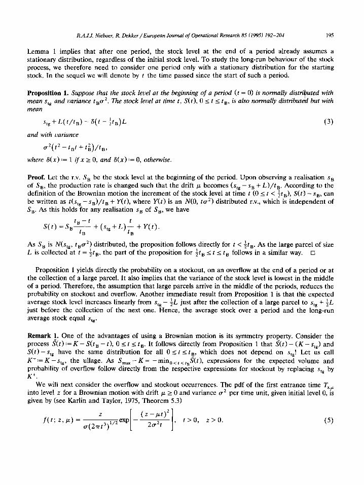
Proposition I. Suppose that the stock level at the beginning o f a period (t = O) is normally distributed with mean stg and variance tBcr 2. The stock level at time t, S( t ), 0 <_ t < t B, is also normally distributed but with mean
Stg + L ( t / t B ) -- 6 ( t -- ½tB)L (3)
and with variance
0-2( t2 -- tat + t2 ) / t B ,
where 6( x ) := 1 i f x >_ O, and 8(x) := 0, otherwise.
Proof. Let the r.v. S B be the stock level at the beginning of the period. Upon observing a realisation s B of S B, the production rate is changed such that the dr i f t /z becomes (stg - s B + L ) / t B. According to the
1 definition of the Brownian motion the increment of the stock level at t ime t (0 < t < ~tB), S( t ) - s a, can be written as t(stg - SB) / t B + Y(t), where Y ( t ) is an N(0, to- z) distributed r.v., which is independent of S B. As this holds for any realisation s B of S B, we have
t B - t t S ( t ) = S B - + ( S t g + L ) - + Y ( t ) .
tB tB
1 As S B is N(stg , tB o'2) distributed, the proposition follows directly for t < ~t B. As the large parcel of size 1 1 L is collected at t = 5t a, the part of the proposition for 5t a < t < t B follows in a similar way. []
Proposition 1 yields directly the probability on a stockout, on an overflow at the end of a period or at the collection of a large parcel. It also implies that the variance of the stock level is lowest in the middle of a period. Therefore, the assumption that large parcels arrive in the middle of the periods, reduces the probability on stockout and overflow. Another immediate result f rom Proposition 1 is that the expected average stock level increases linearly from Stg - ½L just after the collection of a large parcel to Stg + ½L just before the collection of the next one. Hence, the average stock over a period and the long-run average stock equal Stg.
Remark 1. One of the advantages of using a Brownian motion is its symmetry property. Consider the process S(t) := K - S( t B - t), 0 _< t < t B. It follows directly from Proposition 1 that S(t) - (K - sty) and S ( t ) - Stg have the same distribution for all 0 ___ t _< t B, which does not depend on Stg! Let us call K + : = K - s t g , the ullage. As S m ~ - K = - m i n 0 < t < t S(t) , expressions for the expected volume and probability of overflow follow directly from the respective expressions for stockout by replacing Stg by g +"
We will next consider the overflow and stockout occurrences. The pdf of the first entrance time Tz,~, into level z for a Brownian motion with drif t /x ___ 0 and variance 0 -2 per time unit, given initial level 0, is given by (see Karlin and Taylor, 1975, Theorem 5.3)
f ( t ; z , lx) 0-(2.rrt3)l/2exp , t > O , z > O . (5)
196 R.A.J.J. Nieboer, R. Dekker ~European Journal of Operational Research 85 (1995) 192-204
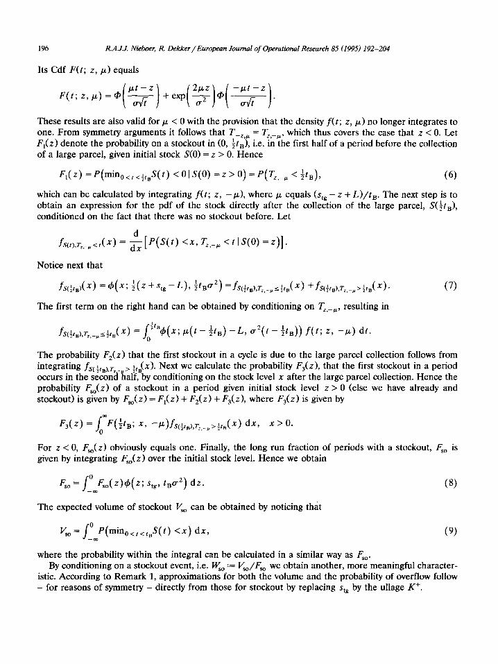
Its Cdf F(t; z, tz) equals
F ( t ; z , l z ) = ~ ~ +expl--- ~ - • trOt-
These results are also valid for/z < 0 with the provision that the density f ( t; z, ~) no longer integrates to one. From symmetry arguments it follows that T_z,~, = Tz,_~,, which thus covers the case that z < 0. Let Fl(Z) denote the probability on a stockout in (0, 1 ~ta), i.e. in the first half of a period before the collection of a large parcel, given initial stock S(0) = z > 0. Hence
1 Fl(z ) = P ( m i n o < t < k t S ( t ) < 0 I S ( 0 ) = z > 0) =P(T~,_~, < ~ts) , (6)
which can be calculated by integrating f ( t; z, -Ix), where/z equals ( s t g - z + L ) / t a. The next step is to obtain an expression for the pdf of the stock directly after the collection of the large parcel, S(½ta), conditioned on the fact that there was no stockout before. Let
fs(t),r~_,<,(x) = ~-~--~[e(s(t) <x , Tz,_~, < t lS (O) = z ) ] .
Notice next that
1 2 fs(½tB)( x ) = ~b(x; ½(z + stg - L ), ~taCr ) = fs(½tB),r~,_ <~,B( X ) + fs(½tB),r~ _~>½t~( X ). (7)
The first term on the right hand can be obtained by conditioning on Tz,_~,, resulting in
!t 1 fs(½t,),rz,_~½t.(x) = fo ~ " ~ b ( x ; / x ( t - ~tB) - L, o ' Z ( / - ½/a)) f(t; z, - / z ) dt .
The probability Fz(z) that the first stockout in a cycle is due to the large parcel collection follows from integrating fs(½t~)r, ~> ½tB(x) • Next we calculate the probability F3(z), that the first stockout in a period occurs in the secon~-~aalf, by conditioning on the stock level x after the large parcel collection. Hence the probability F~o(Z) of a stockout in a period given initial stock level z > 0 (else we have already and stockout) is given by F~o(Z) = Fl(z) + F2(z) + F3(z), where F3(z) is given by
at)
Fa(z ) = f 0 F(½tB; x, )fs(~tB),r~,_,>~t,(x) dx , x - / x , ~ > 0 .
For z < 0, F~o(Z) obviously equals one. Finally, the long run fraction of periods with a stockout, Fso is given by integrating F~o(Z) over the initial stock level. Hence we obtain
Fso= Stg, tB O'2) d z . (8)
The expected volume of stockout V~o can be obtained by noticing that
0 " <t < x ) dx , v~o = f~ P(mm0 <,S(t) (9)
where the probability within the integral can be calculated in a similar way as F~o. By conditioning on a stockout event, i.e. Wso := V~o/F~o we obtain another, more meaningful character-
istic. According to Remark 1, approximations for both the volume and the probability of overflow follow - for reasons of symmetry - directly from those for stockout by replacing stg by the ullage K ÷.
R.A.J.J. Nieboer, R. Dekker / European Journal of Operational Research 85 (1995) 192-204 197
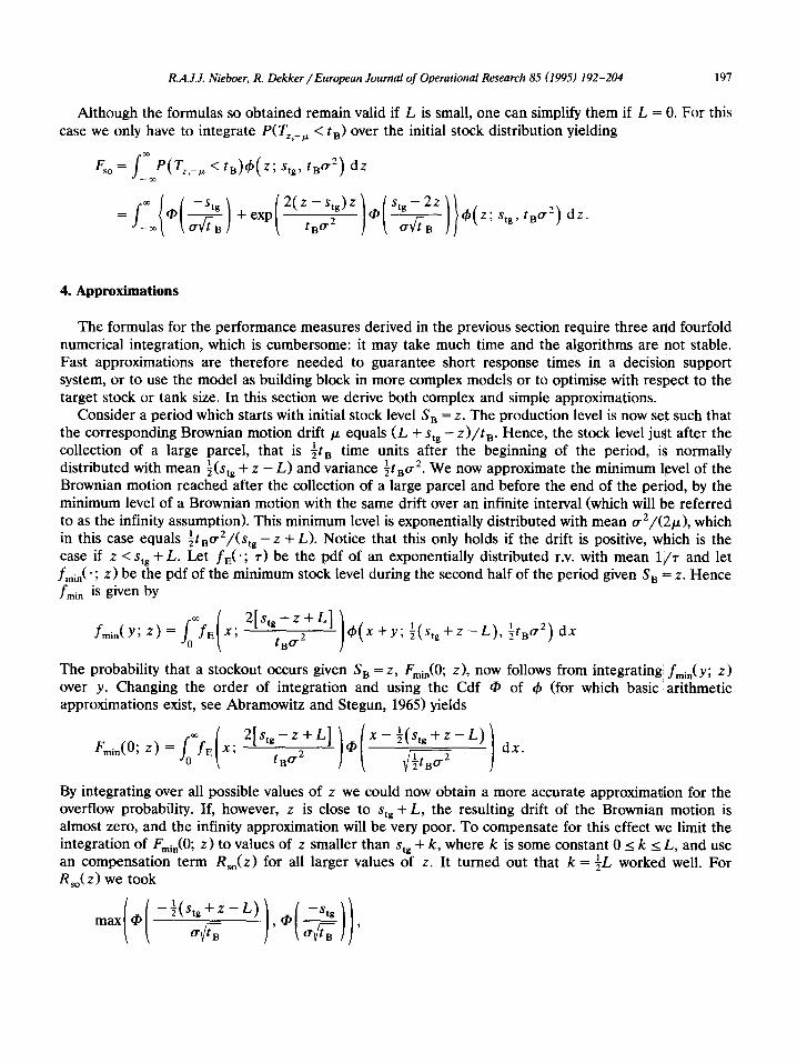
Although the formulas so obtained remain valid if L is small, one can simplify them if L = 0. For this case we only have to integrate P(Tz,_ ~ < t B) over the initial stock distribution yielding
F~o= f ~ P ( T z _ ~ </B)~b(z; stg , /Btr 2) dz
= ~ trv~-B J + e x p - - - tB tr2 q~ ~----V~-B t~(Z; Stg , tBO'2) dz .
4. Approximations
The formulas for the performance measures derived in the previous section require three and fourfold numerical integration, which is cumbersome: it may take much time and the algorithms are not stable. Fast approximations are therefore needed to guarantee short response times in a decision support system, or to use the model as building block in more complex models or to optimise with respect to the target stock or tank size. In this section we derive both complex and simple approximations.
Consider a period which starts with initial stock level Sa = z. The production level is now set such that the corresponding Brownian motion dr i f t /z equals (L + st~ - z ) / t B. Hence, the stock level just after the collection of a large parcel, that is ~t a time units after the beginning of the period, is normally
1 1 2 distributed with mean ~(stg + z - L) and variance ~tatr . We now approximate the minimum level of the Brownian motion reached after the collection of a large parcel and before the end of the period, by the minimum level of a Brownian motion with the same drift over an infinite interval (which will be referred to as the infinity assumption). This minimum level is exponentially distributed with mean trE//(2/x), which in this case equals ½tBtrE//(Stg -- Z + L) . Notice that this only holds if the drift is positive, which is the case if z < stg + L. Let fE( ' ; 7) be the pdf of an exponentially distributed r.v. with mean 1/~" and let fmin( "; z) be the pdf of the minimum stock level during the second half of the period given Sa = z. Hence fmin is given by
fmi . (Y; z) = E X; ~)(X-'by; ~(Stg-J-Z 1 2 tBO "2
The probability that a stockout occurs given S a = z, From(0; z), now follows from integrating fmin(Y, Z) over y. Changing the order of integration and using the Cdf • of th (for which basic:arithmetic approximations exist, see Abramowitz and Stegun, 1965) yields
Fmin(0, z ) = E X; t~ 1 2 tBO" 2 ½~tBtr d x .
By integrating over all possible values of z we could now obtain a more accurate approximation for the overflow probability. If, however, z is close to stg + L, the resulting drift of the Brownian motion is almost zero, and the infinity approximation will be very poor. To compensate for this effect we limit the integration of Fmi~(0; z) to values of z smaller than st~ + k, where k is some constant 0 _< k _<L, and use an compensation term Rso(Z) for all larger values of z. It turned out that k = ½L worked well. For Rso(Z) we took ( ( 1 ) ))
m a x ' ~) "2 ( $tg +t~BZ -- Z ) [ -- Stg
198 R.A.J.J. Nieboer, R. Dekker / European Journal of Operational Research 85 (1995) 192-204
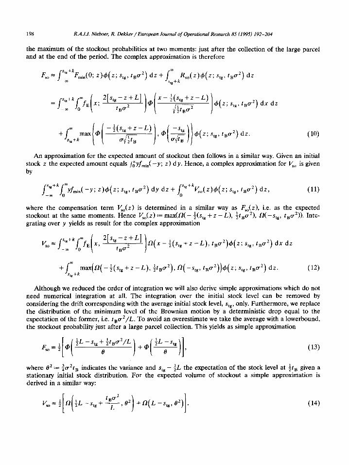
the maximum of the stockout probabilities at two moments: just after the collection of the large parcel and at the end of the period. The complex approximation is therefore
Fso= J o rm~°(O; z )~ (z ; st,, , .o':) dz + (z; ~,.. t.o-:) d~
rs,,+k r= { 2 [ s t g - z + L ] ( /o:EtX; )" ' - L ) X - - ~ - ( S t g -~- Z
1 2
+ f max ~ -- ~(Stg + z - ta o'2) dz. (10)
An approximation for the expected amount of stockout then follows in a similar way. Given an initial stock z the expected amount equals f~Yfmin(-Y; z) dy. Hence, a complex approximation for V~o is given by
stg+k " tB O'2 ) dz rs"+kr~ tBO.Z) d y d z + f ° Vso(Z)d~(z, stg, , J-® Jo Y f m i n ( - - Y ; Z)~(Z'~ Stg , (11)
where the compensation term V~o(Z) is determined in a similar way as F~o(Z), i.e. as the expected stockout at the same moments. Hence V~o(Z).'= ma x ( O( - 1 ~tBo.1 2), ~(Stg + z - L), g2(-Stg, tBcr2)). Inte- grating over y yields as result for the complex approximation
rst,+kr ~ [ 2[s tg - z+L] tj.]( x } l(stg + z - L ) , tBo2)dp(z; Stg, tBo2) dx dz
oo 1 1 2 + f max(g-2(-~(Stg + z - L ), ~tBo" ), g-2(--Stg, tao'2))dp(Z; Stg, tBo'2) dz.
s t g + k
(12)
Although we reduced the order of integration we will also derive simple approximations which do not need numerical integration at all. The integration over the initial stock level can be removed by considering the drift corresponding with the average initial stock level, stg, only. Furthermore, we replace the distribution of the minimum level of the Brownian motion by a deterministic drop equal to the expectation of the former, i.e. tscr2/L. To avoid an overestimate we take the average with a lowerbound, the stockout probability just after a large parcel collection. This yields as simple approximation
f( ) (13, 1 ½L - - Stg "Jr ½tB~r2/L 1 Fs° = 2 q~ 0 +q~ 0 '
where 0 2 3 2 1 := ~cr t B indicates the variance and stg - ½L the expectation of the stock level at ~t~ given a stationary initial stock distribution. For the expected volume of stockout a simple approximation is derived in a similar way:
[( ,B 2 ) o2)) V~o--- ~ a ~ L - s , , + - - 2 - , o 2 + a ( L - s , , , . (14)
R.A.J.J. Nieboer, R. Dekker / European Journal of Operational Research 85 (1995) 192-204 199
5. Optimal capacity and target stock level
O p t i m i s a t i o n with r e spec t to the t a rge t s tock level and the t ank size may be in te res t ing in case of bu i ld ing a new t ank or choos ing a b e t t e r o p e r a t i o n a l policy. In e i the r cases one may min imize a cost funct ion subject to poss ib le service level const ra in ts . Costs may be due to cons t ruc t ing t h e tank, s tock-hold ing , overf low or s tockout . To d e t e r m i n e the tanks ize a two-d imens iona l op t imisa t ion p r o b l e m has to be solved, unless the cost func t ion can be s e pa ra t e d . Not ice tha t the s tockout p robab i l i ty and the expec ted s tockout vo lume d e p e n d only on the t a rge t s tock level, bo th for the exact fo rmulas and the approx ima t ions . T h e s tockhold ing costs, which are a l inear funct ion of the average s tock level, also d e p e n d on the t a rge t stock. H e n c e if the capac i ty costs a re a l inear funct ion of the tanks ize K it is poss ib le to s e p a r a t e the cost func t ion in a pa r t d e p e n d i n g on the t a rge t s tock and a pa r t d e p e n d i n g on the u l lage K +.
6. N u m e r i c a l resu l t s
In this sec t ion the numer i ca l resul ts f rom the app rox ima t ions are discussed. Tab le 1 gives s t a n d a r d va lues of all the p a r a m e t e r s used in the ca lcula t ions . A l t h o u g h they r e p r e s e n t one case only, we be l ieve this case d e m o n s t r a t e s all p rac t ica l re levan t aspects .
Comparison o f the Brownian motion approximations with Poisson simulations
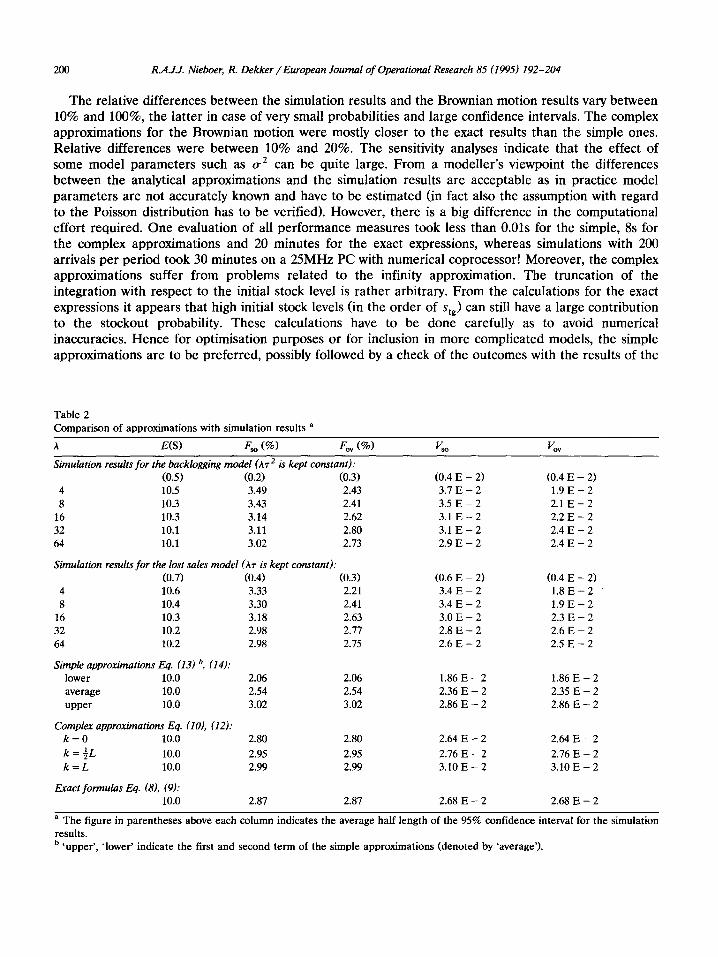
Poisson arr ivals of the smal l cus tomers were s imula ted , bo th for the comple t e back logg ing case as well as for a lost sales (upon s tockout ) and lost p roduc t i on (upon overf low) case. Tab les 2, 3a, 3b and 3c yie ld a c ompa r i son of these resul ts wi th those f rom the Brownian mot ion . Tab le 2 shows the e f f ec t of var ious arr ival ra tes (varying be tween 50 and 800 arr ivals p e r per iod) . In symmetr ic cases (i.e. whe re Stg = K ÷) the s imula t ion resul t s for overf low a re lower than those for s tockout . The exp lana t ion is tha t the Poisson d i s t r ibu t ion is not symmet r i c and has as lower b o u n d zero. This impl ies tha t ex t remely low d e m a n d is less l ikely than ex t r eme ly high d e m a n d , implying tha t an overf low is less l ikely than a s tockout . These d i f fe rences b e c o m e smal l e r if the arr ival ra te A increases , as for l a rge r A the Poisson d i s t r ibu t ion is c loser to a no rma l d is t r ibut ion . T a b l e 2 fu r the r shows tha t the d i f fe rences b e t w e e n the back logging and lost sales cases a re small .
Table 1 Standard values for the parameters
Stg = 10 K = 20 K + = 10 L=10 A=16 ~" =0.2 0 -2 = 0.64 t B = 12.5 Cso = 8.0 E + 3 a
Coy = 4.0 E+3 c h = 10 Ccc = 2 Cvc = 1
Target stock level Capacity of the tank Ullage ( = K - Stg) Size of a large parcel Arrival rate of small parcels Size of small parcels Variance of small demand per time unit ( = k~'2) Length of a period Stockout costs per unit of stockout Overflow costs per unit of overflow Holding costs per unit of stock per unit of time Fixed capacity depreciation costs per unit of time Variable capacity depreciation costs per unit of time
a E denotes the base 10, e.g. E+2 stands for 10 2.
200 R.A.ZJ. Nieboer, R. Dekker / European Journal of Operational Research 85 (1995) 192-204
The relative differences between the simulation results and the Brownian motion results vary between 10% and 100%, the latter in case of very small probabilities and large confidence intervals. The complex approximations for the Brownian motion were mostly closer to the exact results than the simple ones. Relative differences were between 10% and 20%. The sensitivity analyses indicate that the effect of some model parameters such as o -2 can be quite large. From a modeller's viewpoint the differences between the analytical approximations and the simulation results are acceptable as in practice model parameters are not accurately known and have to be estimated (in fact also the assumption with regard to the Poisson distribution has to be verified). However, there is a big difference in the computational effort required. One evaluation of all performance measures took less than 0.01s for the simple, 8s for the complex approximations and 20 minutes for the exact expressions, whereas simulations with 200 arrivals per period took 30 minutes on a 25MHz PC with numerical coprocessor! Moreover, the complex approximations suffer from problems related to the infinity approximation. The truncation of the integration with respect to the initial stock level is rather arbitrary. From the calculations for the exact expressions it appears that high initial stock levels (in the order of Stg) can still have a large contribution to the stockout probability. These calculations have to be done carefully as to avoid numerical inaccuracies. Hence for optimisation purposes or for inclusion in more complicated models, the simple approximations are to be preferred, possibly followed by a check of the outcomes with the results of the
Table 2
Comparison of approximations with simulation results a
A E(S) F~o ( % ) Fo~ ( % ) V~o Vov
Simulation results for the backlogging model (A~ 2 is kept constant): (0.5) (0.2) (0.3) (0.4 E - 2) (0.4 E - 2)
4 10.5 3.49 2.43 3.7 E - 2 1.9 E - 2
8 10.3 3.43 2.41 3.5 E - 2 2.1 E - 2
16 10.3 3.14 2.62 3.1 E - 2 2.2 E - 2
32 10.1 3.11 2.80 3.1 E - 2 2.4 E - 2
64 10.1 3.02 2.73 2.9 E - 2 2.4 E - 2
Simulation results for the lost sales model (Az is kept constant): (0.7) (0.4) (0.3) (0.6 E - 2) (0.4 E - 2)
4 10.6 3.33 2.21 3.4 E - 2 1.8 E - 2
8 10.4 3.30 2.41 3.4 E - 2 1.9 E - 2
16 10.3 3.18 2.63 3.0 E - 2 2.3 E - 2
32 10.2 2.98 2.77 2.8 E - 2 2.6 E - 2
64 10.2 2.98 2.75 2.6 E - 2 2.5 E - 2
Simple approximations Eq. (13) b, (14): lower 10.0 2.06 2.06 1.86 E - 2 1.86 E - 2
average 10.0 2.54 2.54 2.36 E - 2 2.35 E - 2
upper 10.0 3.02 3.02 2.86 E - 2 2.86 E - 2
Complex approximations Eq. (10), (12): k = 0 10.0 2.80 2.80 2.64 E - 2 2.64 E - 2
1 k = 7 L I0.0 2.95 2.95 2.76 E - 2 2.76 E - 2
k = L 10.0 2.99 2.99 3.10 E - 2 3.10 E - 2
Exact formulas Eq. (8), (9): 10.0 2.87 2.87 2.68 E - 2 2.68 E - 2
a The figure in parentheses above each column indicates the average half length of the 95% confidence interval for the simulation results. b 'upper', 'lower' indicate the first and second term of the simple approximations (denoted by 'average').
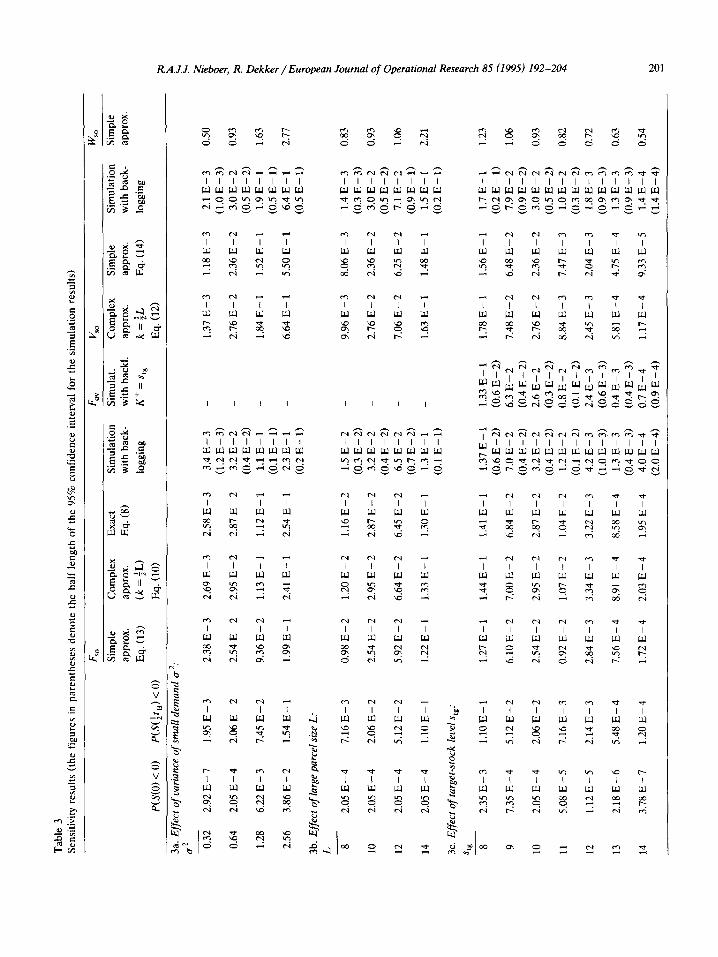
Tab
le 3
Sen
siti
vity
res
ults
(th
e fi
gu
res
in p
aren
thes
es
den
ote
th
e h
alf
len
gth
of
the
95
% c
on
fid
ence
in
terv
al f
or
the
sim
ula
tio
n r
esu
lts)
P(S
(O)
< O
) P
(S(½
t B)
< O
)
F~o
Fo~
Ko
Sim
ple
C
om
ple
x
Ex
act
Sim
ula
tio
n
Sim
ula
t.
Co
mp
lex
app
rox
, ap
pro
x.
Eq
. (8
) w
ith
bac
k-
wit
h b
ack
l,
app
rox
.
Eq
. (1
3)
(k =
½L
) lo
gg
ing
K
+ =
Stg
k
= ½
L
Eq
. (1
0)
Eq
. (1
2)
Sim
ple
app
rox
.
Eq
. (1
4)
Sim
ula
tio
n
wit
h b
ack
-
log
gin
g
~o
Sim
ple
app
rox
.
3a.
Eff
ect
of v
aria
nce
of s
mal
l de
man
d o-
2..
O- 2
0.32
2.
92 E
-
7 1.
95 E
-
3
0.64
2.
05 E
-
4 2.
06 E
-
2
1.28
6.
22 E
-
3 7.
45 E
-
2
2.56
3.
86 E
-
2 1.
54 E
-
1
3b.
Eff
ect
of la
rge
parc
el s
ize
L:
L 8 2.
05 E
-4
7.16
E-3
10
2.05
E -
4
2.06
E -
2
12
2.05
E-4
5.
12 E
-2
14
2.05
E-4
1.
10 E
-1
3c.
Eff
ect
of ta
rget
-sto
ck l
evel
Sts
.
Stg 8
2.35
E -
3
1.10
E-
1
9 7.
35 E
-4
5.12
E-2
10
2.05
E -
4
2.06
E -
2
ll
5.08
E-5
7.
16 E
-3
12
1.12
E-5
2.
14 E
-3
13
2.18
E-6
5.
48 E
-4
14
3.78
E -
7
1.20
E -
4
2.38
E-3
2.
69 E
-3
2.58
E-3
3.
4 E
-3
(1.2
E-3
)
2.54
E -
2
2.95
E -
2
2.87
E -
2
3.2
E -
2
(0.4
E-
2)
9.36
E-2
1.
13 E
-1
1.1
2E
-1
1.1
E-1
(0.1
E-
1)
1.99
E -
1
2.41
E -
1
2.54
E-
1 2.
3 E
- 1
(0.2
E -
1)
0.98
E-2
1.
20 E
-2
1.16
E-2
1.
5 E
-2
(0.3
E -
2)
2.54
E -
2
2.95
E -
2
2.87
E -
2
3.2
E -
2
(0.4
E -
2)
5.92
E -
2
6,64
E -
2
6.45
E -
2
6.5
E -
2
(0.7
E -
2)
1.22
E-
1 1.
33 E
-
1 1.
30 E
- 1
1.3
E -
1
(0.1
E -
1)
1.37
E -
3
2.76
E -
2
1.84
E-
1
6.64
E-
1
9.96
E -
3
2.76
E -
2
7.06
E -
2
1.63
E -
1
1.18
E-3
2.36
E -
2
1.52
E-
1
5.50
E-
1
8.06
E -
3
2.36
E-
2
6.25
E -
2
1.48
E -
1
2.1
E-3
(1.0
E-
3)
3.0
E-2
(0.5
E -
2)
1.9
E-
1
(0.5
E -
1)
6.4
E-1
(0.5
E-
1)
1.4
E-3
(0.3
E-
3)
3.0
E-2
(0.5
E -
2)
7.1
E-2
(0.9
E-
1)
1.5
E-
i
(0.2
E-
1)
1.27
E -
1
1.44
E-
1 1.
41 E
- 1
1.37
E -
1
1.33
E-
1 1.
78 E
-
1 1.
56 E
- 1
1.7
E-
1
(0.6
E -
2)
(0
.6 E
-
2)
(0.2
E -
1)
6,10
E-2
7.
00 E
-2
6.84
E-2
7.
0 E
-2
6.3
E-2
7.
48 E
-2
6.48
E-2
7.
9 E
-2
(0.4
E-
2)
(0.4
E-
2)
(0.9
E-
2)
2.54
E -
2
2.95
E -
2
2.87
E -
2
3.2
E -
2
2.6
E -
2
2.76
E -
2
2.36
E -
2
3.0
E -
2
(0.4
E -
2)
(0
.3 E
-
2)
(0.5
E -
2)
0.92
E -
2
1.07
E -
2
1.04
E -
2
1.2
E -
2
0.8
E -
2
8.84
E -
3
7.47
E -
3
1.0
E -
2
(0.1
E-2
) (0
.1 E
-2)
(0.3
E-2
)
2.84
E -
3
3.34
E -
3
3.22
E -
3
4.2
E -
3
2.4
E -
3
2.45
E -
3
2.04
E -
3
1.8
E -
3 (1
.0 E
-
3)
(0.6
E -
3)
(0
.9 E
-
3)
7.56
E-4
8
.91
E-4
8.
58 E
-4
1.3
E-3
0.
4 E
-3
5.8
1E
-4
4.75
E-4
1.
3 E
-3
(0.4
E-3
) (0
.4 E
-3
) (0
.9 E
-3)
1.72
E-4
2.
03 E
-4
1.95
E-4
4.
0 E
-4
0.7
E-4
1.
17 E
-4
9.33
E-5
1.
4 E
-4
(2.0
E -
4)
(0
.9 E
-
4)
(1.4
E -
4)
0.50
0.93
1.63
2.77
0.83
0.93
1.06
2.21
1.23
1.06
0.93
0.82
0.72
0.63
0.54
I t,~
202 R.4.J.J. Nieboer, R. Dekker / European Journal of Operational Research 85 (1995) 192-204
complex approximat ions or s imulat ion. The exact expressions should be used if the large parcel size is very small or zero.
Sensitivity results
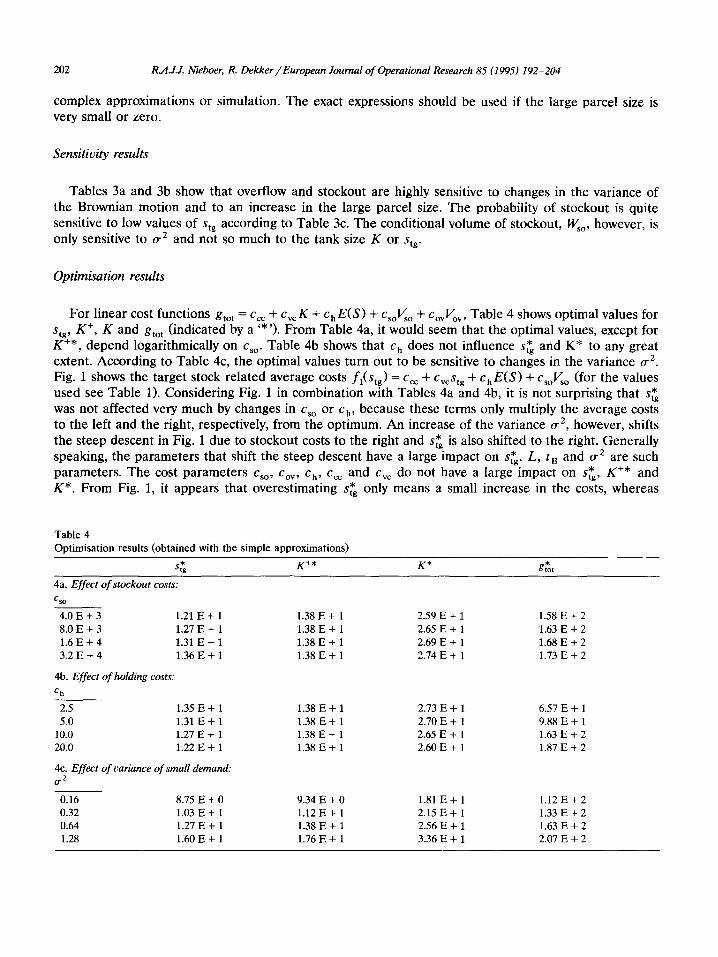
Tables 3a and 3b show that overflow and stockout are highly sensitive to changes in the var iance of the Brownian mot ion and to an increase in the large parcel size. The probabil i ty of stockout is qui te sensitive to low values of stg according to Table 3c. The condi t ional volume of stockout, W~o, however, is only sensitive to tr 2 and not so much to the tank size K or Stg.
Optimisation results
For l inear cost funct ions gtot = Ccc + cvcK + ChE(S) + csoV~o + CovVov, Table 4 shows opt imal values for Stg, K ÷, K and gtot ( indicated by a '* ') . F rom Table 4a, it would seem that the opt imal values, except for
* and K* to any great K ÷*, d e p e n d logari thmically on Cso. Table 4b shows that c h does not inf luence stg extent. Accord ing to Table 4c, the opt imal values tu rn out to be sensitive to changes in the var iance 0 -2.
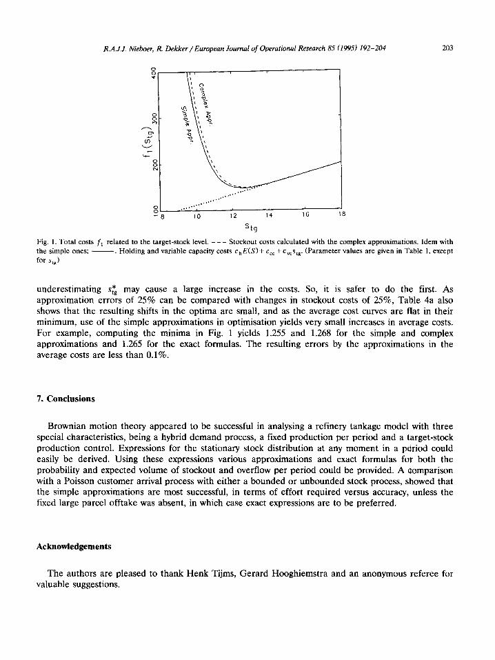
Fig. 1 shows the target stock re la ted average costs fl(Stg) = Ccc + CvcStg + ChE(S) + csoVso (for the values used see Table 1). Cons ider ing Fig. 1 in combina t ion with Tables 4a and 4b, it is not surpris ing that S~g was not affected very much by changes in Cso or c h, because these terms only mult iply the average costs to the left and the right, respectively, from the op t imum. A n increase of the var iance or 2, however, shifts
* is also shifted to the right. Genera l ly the steep descent in Fig. 1 due to s tockout costs to the right and stg speaking, the pa ramete r s that shift the steep descent have a large impact on S~g. L, t B and o "z are such
parameters . The cost pa ramete rs C~o, Cov, Ch, C~c and cv~ do not have a large impact on sty, K +* and K*. F rom Fig. 1, it appears that overes t imat ing st~ only means a small increase in the costs, whereas
Table 4 Optimisation results (obtained with the simple approximations)
st~ K +* K* * gtot
4a. Effect of stockout costs: CSO
4.0E+ 3 1.21 E+ 1 1.38 E + 1 2.59 E + 1 1.58 E + 2 8.0 E+ 3 1.27 E + 1 1.38 E + 1 2.65 E + 1 1.63 E + 2 1.6E+4 1.31 E+ 1 1.38E+ 1 2.69E+ 1 1.68 E + 2 3.2 E + 4 1.36 E + 1 1.38 E + 1 2.74 E + 1 1.73 E + 2
4b. Effect of holding costs: Ch
2.5 1.35 E + 1 1.38 E + 1 2.73 E + 1 6.57 E + 1 5.0 1.31 E + 1 1.38 E + 1 2.70 E + 1 9.88 E + 1
10.0 1.27 E + 1 1.38 E + 1 2.65 E + 1 1.63 E + 2 20.0 1.22 E + 1 1.38 E + 1 2.60 E + 1 1.87 E + 2
4c. Effect of variance of small demand: 0.2
0.16 8.75 E + 0 9.34 E + 0 1.81 E + 1 1.12 E + 2 0.32 1.03 E + 1 1.12 E + 1 2.15 E + 1 1.33 E + 2 0.64 1.27 E + 1 1.38 E + 1 2.56 E + 1 1.63 E + 2 1.28 1.60 E + 1 1.76 E + 1 3.36 E + 1 2.07 E + 2
R.A.J.J. Nieboer, R. Dekker / European Journal of Operational Research 85 (1995) 192-204 203
0
o
O3
~ 8 16 18
~ O I o
. , . , * ' °
° . . . . . .
m ' " ' " i i i
10 12 14
$lq
Fig. 1. Total costs fl related to the target-stock level. - - - Stockout costs calculated with the complex approximations. Idem with the simple ones; - - . Holding and variable capacity costs chE(S)+ Ccc + cvcstg. (Parameter values are given in Table 1, except for stg)
underest imating st~ may cause a large increase in the costs. So, it is safer to do the first. As approximation errors of 25% can be compared with changes in stockout costs of 25%, Table 4a also shows that the resulting shifts in the opt ima are small, and as the average cost curves are nat in their minimum, use of the simple approximations in optimisation yields very small increases in average costs. For example, computing the minima in Fig. 1 yields 1.255 and 1.268 for the simple and complex approximations and 1.265 for the exact formulas. The resulting errors by the approximations in the average costs are less than 0.1%.
7, Conclusions
Brownian motion theory appeared to be successful in analysing a refinery tankage model with three special characteristics, being a hybrid demand process, a fixed production per period and a target-stock production control. Expressions for the stationary stock distribution at any moment in a period could easily be derived. Using these expressions various approximations and exact formulas for both the probability and expected volume of stockout and overflow per period could be provided. A comparison with a Poisson customer arrival process with either a bounded or unbounded stock process, showed that the simple approximations are most successful, in terms of effort required versus accuracy, unless the fixed large parcel offtake was absent, in which case exact expressions are to be preferred.
Acknowledgements
The authors are pleased to thank Henk Tijms, Gerard Hooghiemstra and an anonymous referee for valuable suggestions.
204 R,4.J.J. Nieboer, R. Dekker ~European Journal of Operational Research 85 (1995) 192-204
References
Abramowitz, M., and Stegun, I.A. (1965). Handbook of Mathematical Functions, Dover, New York. Karlin, S., and Taylor, H.M. (1975), A First Course in Stochastic Processes, 2nd ed., Academic Press, New York. Klingman, D., Phillips, N., Steiger, D., Wirth, R., Padman, R., and Krishnan, R. (1987), "An optimization-based integrated
short-term refined petroleum product planning system", Management Science 33, 813-830. Langeveld, A.T. (1989), "Downstream Oil and Chemicals Logistic Conference: Where ends have to meet', in: C.F.H. van Rijn (ed.),
Logistics: Where Ends Have to Meet, Pergamon, Oxford. Miltenburg, G.J. (1987), "Co-ordinated control of a family of discount-related items", Canadian Journal of Operations Research and
Information Processing 25, 97-116. Miltenburg, G.J., and Silver, E.A. (1984), "Accounting for residual stock in continuous review coordinated control of a family of
items", International Journal of Production Research 22, 607-628. Miltenburg, G.J., and Silver, E.A. (1984), "The diffusion process and residual stock in periodic review coordinated control of
families of items", International Journal of Production Research 22, 629-646. Odi, T.O., and Karimi, I.A. (1988), "Sizing of intermediate storage for variabilities in noncontinuous processes with parallel units",
Computers and Chemical Engineering 12, 561-572. Shreve, S.E., Lehoczky, J.P., and Gaver, D.P. (1984), "Optimal consumption for general diffusions with absorbing and reflecting
barriers", SlAM Journal on Control and Optimization 22, 55-75.