BROUWER’S FIXED-POINT THEOREM IN PLANE GEOMETRY · This theorem is a special case of Brouwer’s Fixed-Point Theorem, and it is proven by directly repeating the transformation

International Journal of Academic Research and Reflection Vol. 6, No. 1, 2018 ISSN 2309-0405

Progressive Academic Publishing, UK Page 1 www.idpublications.org

BROUWER’S FIXED-POINT THEOREM IN PLANE GEOMETRY

Sukru ILGUN

Assistant Professor, Kafkas University, Education Faculty, Mathematics Education Department

Office ZA106 Kars, TURKIYE

E-mail address of the corresponding author: [email protected]

ABSTRACT

This study is about the proof of the theorem known as the first basic Fixed-Point Theorem

found by L. E. J. Brouwer between the year 1909 and 1913 in plane geometry. As known,

there have been other studies on fixed-point after Brouwer, other theorems were presented,

proven and brought into the literature. When we look at these theorems, we see that they are

usually used by fields such as analysis and topology in Turkey and abroad as significant tools

with applications. In this article on the other hand, we will prove Brouwer’s theorem that ‘C

being a unit sphere on nR there is a fixed-point for the function f: C → C in continuous

transformation [7],’ using concepts of expansions/compressions, pushes and rotations in

plane geometry.

Keywords: Fixed-Point Theorem, Plane Geometry, Expansion/Compression, Push, Rotation

1. INTRODUCTION and DEFİNİTİONS

Firstly, we would like to begin with a short history of fixed point theory as it can be also seen

in the works of Lennard and Nezir [14,15]. Researches on fixed point theory initiated in 1912

by L.E.J. Brouwer ‘s result [2]. Brouwer showed that for n N , for C the set of the closed

unit ball of nR every norm-to-norm continuous function :f C C has a fixed point. Later,

in 1930 Schauder [16] generalized Brouwer’s result to every compact convex subset of nR

This class of continuous functions was very large and so researches wanted to work on

smaller classes of the functions and researched fixed points of those. Then, in 1922, the well-

known fixed point theorem arrived. Banach gave his theorem so called Banach Contraction

theorem [1] as follows: if ( , )X d is a complete metric space and :f X X is a strict

contraction for the metric .

d d generated by the norm, then f has a unique fixed point.

Later, more technical theorems were proven by other researches. Indeed, 1965 was very

efficient year for the fixed point theory and in this year, there were three big results for this

field by Browder, Gothe and Kirk.

In 1965, Browder [3] proved : (For every closed, bounded, convex (non-empty) subset C of a

Hilbert space (X, . ), for all nonexpansive mappings T: C → C (i.e., Tx Ty ≤ x y ,

for all x, y), T has a fixed point in C.) Soon after, also in 1965, Browder and Göhde

(independently) generalized the result to uniformly convex Banach space (X, . ), e.g., X= pL

, 1< p < ∞ , with its usual norm . p .

Later in 1965,Kirk [11] further generalised to all reflexive Banach space X with normal

structure: those spaces such that all-trivial closed, bounded, convex sets C have a smaller

radius than diameter.

Spaces (X, . ) with the property of Browder became known as spaces with the “fixed point

property for nonexpansive mappings” (FPP(n.e)).After 48 years, it remains an open question



as to whether or not every reflexive Banach space (X, . ) has the fixed point property for

nonexpansive mappings.

In 1960 Kutuzov B.V. mentioned the transformation of shapes and stable points of these

shapes in his book named Geometry, studies in Mathematics Vol. IV [13]

Again, in 1973 S.R. Clemens published an article named Fixed Point Theorems in Euclidean

Geometry. In this article he explained how Euclidean Geometry Fixed Point works. He also

showed Menelaus and Seva Theorems are good application of Fixed Point Theorem. [4]

In our study, we stressed on examples of plane geometry of L.E.J. Brouwer Fixed Point

Theorem. Our purpose is to bring plane geometry into the research conducted on fixed-points

and open up a new field.

1.1. Definition (Fixed-Point): Let X be a non-empty set, and T: X → X a function. If there is

at least one x ∈ X that satisfies T(x) = x, x is a fixed point of the function T. All x ∈ X

satisfying this equality are fixed-points of the function T [15].

1.2. Definition (Compressive Transformation): Let (X, d) be a metric space and T: X → X

any transformation (function). If for all x, y X, there is a number α (0 ≤ α < 1) satisfying

d(Tx, Ty) ≤ α.d(x, y), T is called a compressive transformation [15].

1.3. Definition (Closed Unit Sphere): The subset B d(x, 1) Rn for ∀ n ∈ N is called a

closed unit sphere of radius 1 with the center x in Rn.

It is defined as B d(x, 1) = {y ∈ Rn⋮ d(x, y) ≤ 1, x ∈ R

n} [8].

1.4. Definition (Expansion-Dilation): The similarity transformation mapping parallel lines

to parallel lines and preserving direction is called a dilation. This transformation is also a

collineation, mapping points to points, lines to lines, and planes to planes [5].

1.5. Definition:

1. Expansion/compression transformation for a point (x, y) in a plane is defined as

Gk(x, y) = (kx, ky) while k ∈ [0, 1) [15].

2. Counterclockwise rotation of as point (x, y) in a plane by θ is defined as

Rθ(x, y) = cos sin

sin cos

.x

y

[9].

3. Pushing a point (x, y) in a plane is defined as V

T (x, y) = (x + a, y + b) while V (a, b)

is the pushing vector [9].

1.1. Theorem (Brouwer’s Fixed-Point Theorem):

While any C = B d(x, 1) Rn

having x ∈ R

n for ∀ n ∈ N is a closed unit sphere, the

continuous transformation T: C → C has a fixed-point. That is, any continuous

transformation mapping Rn’s closed unit sphere to itself has a fixed-point [7].

1.1. Proof: For the continuous transformation f: [a, b] → [a, b] while C = [a, b], there exists

x ∈ [a, b] satisfying f(x) = x.

If we take F(x) = x – f(x), and let F(a) = a – f(a) ≤ 0 and F(b) = b – f(b) ≥ 0, according to the

intermediate value theorem, there is at least one x ∈ [a, b] such that F(x) = 0. If F(x) = 0, then

x – f(x) = 0, meaning f(x) = x.

Q.E.D. [10].



2. MAİN RESULTS

It is possible to provide various proofs of Brouwer’s Fixed-Point Theorem using analysis and

topology. In our study, we will provide one proof from analysis and demonstrate other proofs

over plane geometry. The proof of plane geometry mentioned above stated in four diffent

ways as main result.

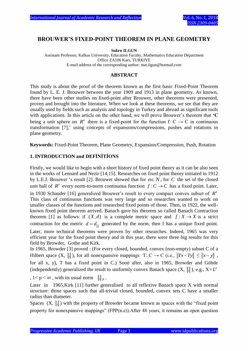
Proof 2.1: Let us chose our C closed sphere as a square and define our continuous

transformation f as f: C→ Cl, mapping the closed square to another square. Let us show that

this transformation has at least one fixed-point.

The transformation, while mapping points from the bigger square to the smaller square,

leaves at least one point fixed. We will first try to demonstrate how such a fixed-point is

found, and then try to see whether such a transformation can be explained by an equation.

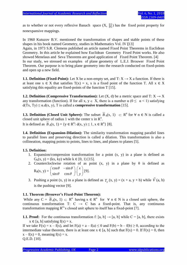
Proof 2.2:

C

X

Y

Cl



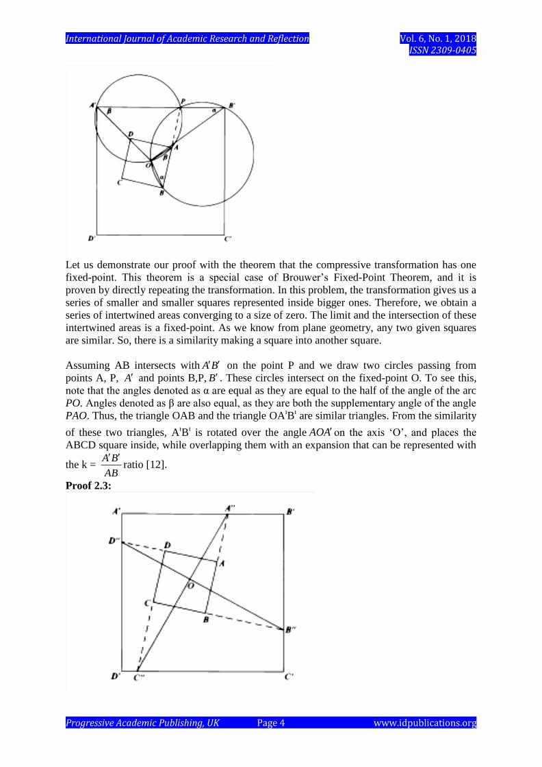
Let us demonstrate our proof with the theorem that the compressive transformation has one

fixed-point. This theorem is a special case of Brouwer’s Fixed-Point Theorem, and it is

proven by directly repeating the transformation. In this problem, the transformation gives us a

series of smaller and smaller squares represented inside bigger ones. Therefore, we obtain a

series of intertwined areas converging to a size of zero. The limit and the intersection of these

intertwined areas is a fixed-point. As we know from plane geometry, any two given squares

are similar. So, there is a similarity making a square into another square.

Assuming AB intersects with A B on the point P and we draw two circles passing from

points A, P, A and points B,P, B . These circles intersect on the fixed-point O. To see this,

note that the angles denoted as α are equal as they are equal to the half of the angle of the arc

PO. Angles denoted as β are also equal, as they are both the supplementary angle of the angle

PAO. Thus, the triangle OAB and the triangle OAıB

ı are similar triangles. From the similarity

of these two triangles, AıB

ı is rotated over the angle AOAon the axis ‘O’, and places the

ABCD square inside, while overlapping them with an expansion that can be represented with

the k = A B

AB

ratio [12].

Proof 2.3:



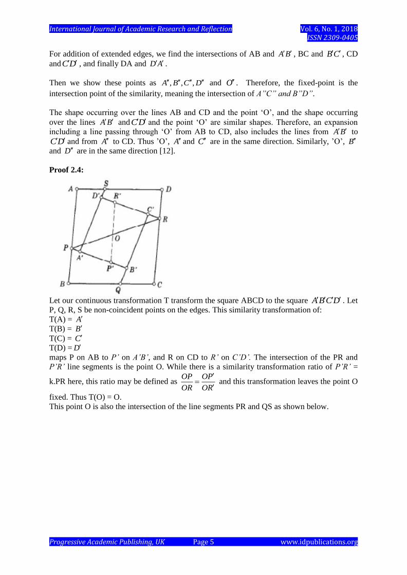
For addition of extended edges, we find the intersections of AB and A B , BC and B C , CD

andC D , and finally DA and D A .

Then we show these points as , , ,A B C D and O . Therefore, the fixed-point is the

intersection point of the similarity, meaning the intersection of A”C” and B”D”.

The shape occurring over the lines AB and CD and the point ‘O’, and the shape occurring

over the lines A B andC D and the point ‘O’ are similar shapes. Therefore, an expansion

including a line passing through ‘O’ from AB to CD, also includes the lines from A B to

C D and from A to CD. Thus ’O’, A and C are in the same direction. Similarly, ’O’, B

and D are in the same direction [12].

Proof 2.4:

Let our continuous transformation T transform the square ABCD to the square A B C D . Let

P, Q, R, S be non-coincident points on the edges. This similarity transformation of:

T(A) = A

T(B) = B

T(C) = C T(D) = D

maps P on AB to P’ on A’B’, and R on CD to R’ on C’D’. The intersection of the PR and

P’R’ line segments is the point O. While there is a similarity transformation ratio of P’R’ =

k.PR here, this ratio may be defined as OP OP

OR OR

and this transformation leaves the point O

fixed. Thus T(O) = O.

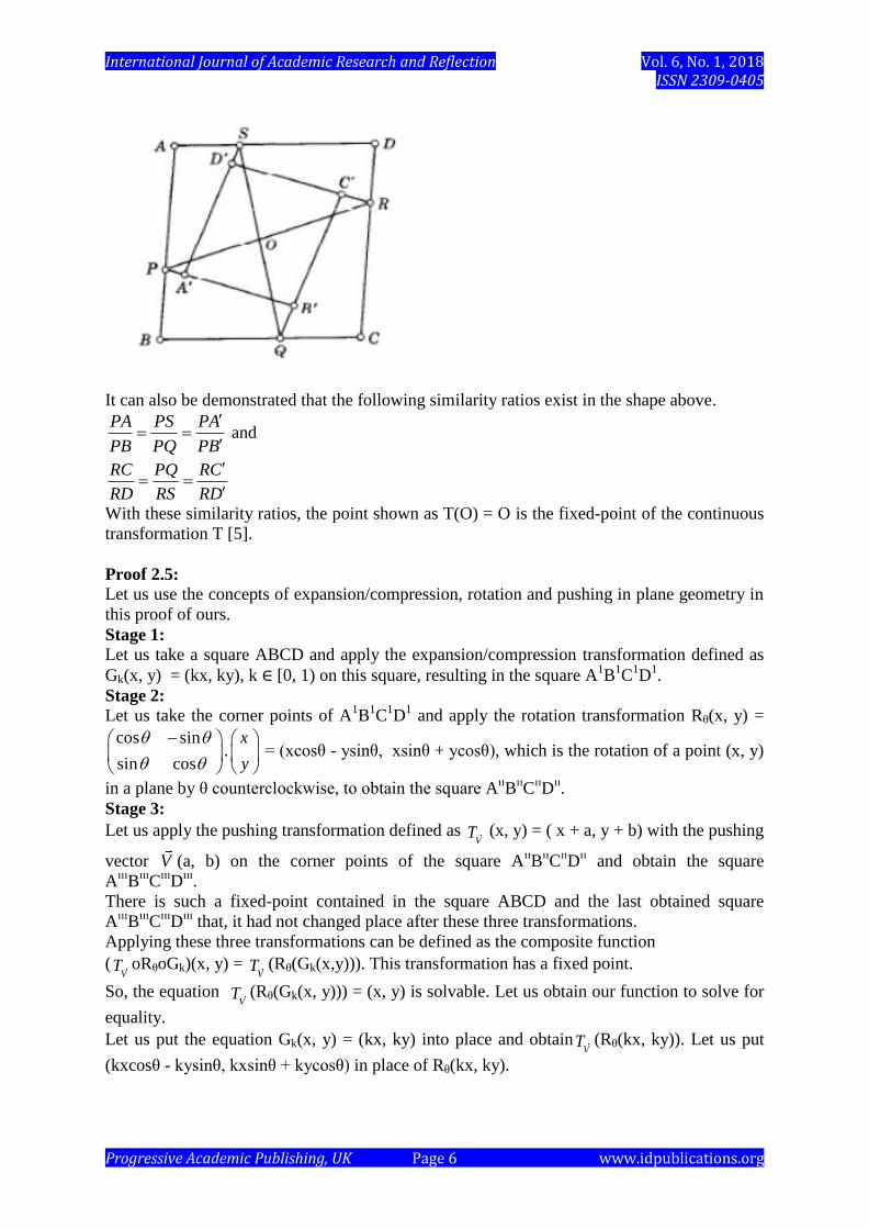
This point O is also the intersection of the line segments PR and QS as shown below.



It can also be demonstrated that the following similarity ratios exist in the shape above.

PA PS PA

PB PQ PB

and

RC PQ RC

RD RS RD

With these similarity ratios, the point shown as T(O) = O is the fixed-point of the continuous

transformation T [5].

Proof 2.5: Let us use the concepts of expansion/compression, rotation and pushing in plane geometry in

this proof of ours.

Stage 1: Let us take a square ABCD and apply the expansion/compression transformation defined as

Gk(x, y) = (kx, ky), k ∈ [0, 1) on this square, resulting in the square A1B

1C

1D

1.

Stage 2: Let us take the corner points of A

1B

1C

1D

1 and apply the rotation transformation Rθ(x, y) =

cos sin

sin cos

.x

y

= (xcosθ - ysinθ, xsinθ + ycosθ), which is the rotation of a point (x, y)

in a plane by θ counterclockwise, to obtain the square AııB

ııC

ııD

ıı.

Stage 3:

Let us apply the pushing transformation defined as V

T (x, y) = ( x + a, y + b) with the pushing

vector V (a, b) on the corner points of the square AııB

ııC

ııD

ıı and obtain the square

Aııı

Bııı

Cııı

Dııı

.

There is such a fixed-point contained in the square ABCD and the last obtained square

Aııı

Bııı

Cııı

Dııı

that, it had not changed place after these three transformations.

Applying these three transformations can be defined as the composite function

(V

T oRθoGk)(x, y) = V

T (Rθ(Gk(x,y))). This transformation has a fixed point.

So, the equation V

T (Rθ(Gk(x, y))) = (x, y) is solvable. Let us obtain our function to solve for

equality.

Let us put the equation Gk(x, y) = (kx, ky) into place and obtainV

T (Rθ(kx, ky)). Let us put

(kxcosθ - kysinθ, kxsinθ + kycosθ) in place of Rθ(kx, ky).



Our statement is now V

T (kxcosθ - kysinθ, kxsinθ + kycosθ). Computing for this statement,

we obtain the equation (V

T oRθoGk)(x, y) = (a + kxcosθ - kysinθ, b + kxsinθ + kycosθ ) = (x,

y). We have obtained two first degree equations and their solution is simple.

Let us organize the equations a + kxcosθ - kysinθ = x and b + kxsinθ + kycosθ = y.

a = (1 - kcosθ)x + kysinθ ……….(1 )

b = (1 - kcosθ)y - kxsinθ ……….( 2)

These equations can be solved with the elimination method. The point (x, y) obtained with

this solution is the fixed-point of the transformation defined between two squares [6].

EXAMPLE:

This section will demonstrate that the composite transformation obtained above is a

transformation that has a fixed-point for any random square.

Let A(8 2 , 8 2 ), B(8 2 , -8 2 ), C(-8 2 , -8 2 ) and D(-8 2 , 8 2 ) be the corner

points of the square ABCD.

Stage 1:

Let us apply the expansion/compression transformation of: 1

8

G (x, y) = ( 1

8x,

1

8x),

transforming the square ABCD to the square AıB

ıC

ıD

ı.

We obtain the points Aı( 2 , 2 ), B

ı( 2 , 2 ), C

ı( 2 , 2 ) and D

ı( 2 , 2 ).

Stage 2:

Let us rotate the square AıB

ıC

ıD

ı counterclockwise around the origin by 45 .

By substituting 45 for θ in the transformation Rθ(x, y)= cos sin

sin cos

.x

y

, we obtain

the square AııB

ııC

ııD

ıı.

Aıı(0, 2), B

ıı(2 ,0), C

ıı(0, -2) and D

ıı(-2, 0) are the corner points of the square A

ııB

ııC

ııD

ıı.

Stage 3:Let us apply the transformation of pushing the corners of the square AııB

ııC

ııD

ıı to the

right by 2 units and upwards by 2 units, obtaining the square Aııı

Bııı

Cııı

Dııı

as a result. The

corner points of this square can be found as:

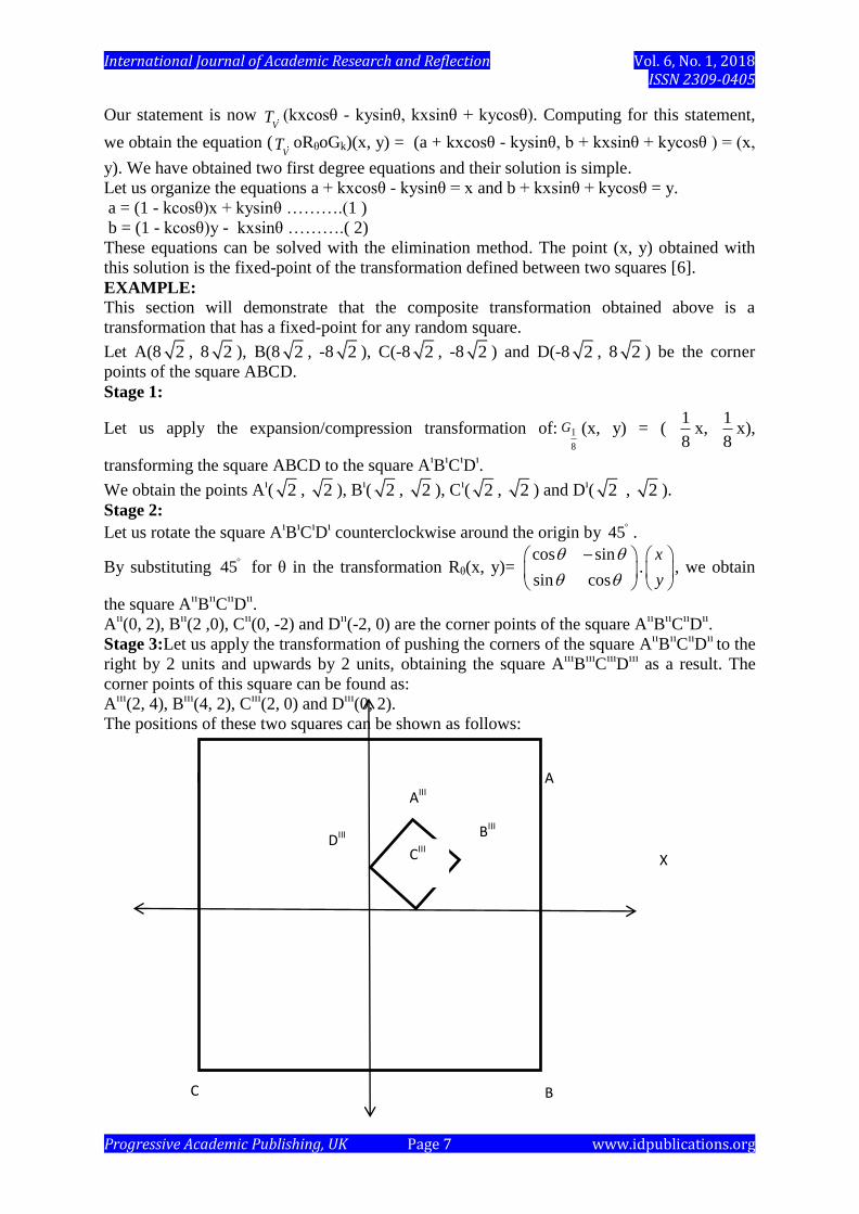
Aııı

(2, 4), Bııı

(4, 2), Cııı

(2, 0) and Dııı

(0, 2).

The positions of these two squares can be shown as follows:

X

B C

D

Y

A

CIII DIII BIII

AIII



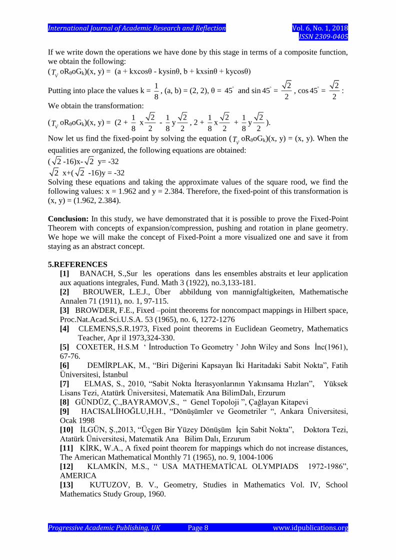
If we write down the operations we have done by this stage in terms of a composite function,

we obtain the following:

(V

T oRθoGk)(x, y) = (a + kxcosθ - kysinθ, b + kxsinθ + kycosθ)

Putting into place the values k = 1

8, (a, b) = (2, 2), θ = 45 and sin 45 =

2

2, cos 45 =

2

2:

We obtain the transformation:

(V

T oRθoGk)(x, y) = (2 + 1

8 x

2

2 -

1

8y

2

2, 2 +

1

8x

2

2 +

1

8y

2

2).

Now let us find the fixed-point by solving the equation (V

T oRθoGk)(x, y) = (x, y). When the

equalities are organized, the following equations are obtained:

( 2 -16)x- 2 y= -32

2 x+( 2 -16)y = -32

Solving these equations and taking the approximate values of the square rood, we find the

following values: x = 1.962 and y = 2.384. Therefore, the fixed-point of this transformation is

(x, y) = (1.962, 2.384).

Conclusion: In this study, we have demonstrated that it is possible to prove the Fixed-Point

Theorem with concepts of expansion/compression, pushing and rotation in plane geometry.

We hope we will make the concept of Fixed-Point a more visualized one and save it from

staying as an abstract concept.

5.REFERENCES

[1] BANACH, S.,Sur les operations dans les ensembles abstraits et leur application

aux aquations integrales, Fund. Math 3 (1922), no.3,133-181.

[2] BROUWER, L.E.J., Über abbildung von mannigfaltigkeiten, Mathematische

Annalen 71 (1911), no. 1, 97-115.

[3] BROWDER, F.E., Fixed –point theorems for noncompact mappings in Hilbert space,

Proc.Nat.Acad.Sci.U.S.A. 53 (1965), no. 6, 1272-1276

[4] CLEMENS,S.R.1973, Fixed point theorems in Euclidean Geometry, Mathematics

…… Teacher, Apr il 1973,324-330.

[5] COXETER, H.S.M ‘ İntroduction To Geometry ’ John Wiley and Sons İnc(1961),

67-76.

[6] DEMİRPLAK, M., “Biri Diğerini Kapsayan İki Haritadaki Sabit Nokta”, Fatih

Üniversitesi, İstanbul

[7] ELMAS, S., 2010, “Sabit Nokta İterasyonlarının Yakınsama Hızları”, Yüksek

Lisans Tezi, Atatürk Üniversitesi, Matematik Ana BilimDalı, Erzurum

[8] GÜNDÜZ, Ç.,BAYRAMOV,S., “ Genel Topoloji ”, Çağlayan Kitapevi

[9] HACISALİHOĞLU,H.H., “Dönüşümler ve Geometriler “, Ankara Üniversitesi,

Ocak 1998

[10] İLGÜN, Ş.,2013, “Üçgen Bir Yüzey Dönüşüm İçin Sabit Nokta”, Doktora Tezi,

Atatürk Üniversitesi, Matematik Ana Bilim Dalı, Erzurum

[11] KİRK, W.A., A fixed point theorem for mappings which do not increase distances,

The American Mathematical Monthly 71 (1965), no. 9, 1004-1006

[12] KLAMKİN, M.S., “ USA MATHEMATİCAL OLYMPIADS 1972-1986”,

AMERICA

[13] KUTUZOV, B. V., Geometry, Studies in Mathematics Vol. IV, School

Mathematics Study Group, 1960.



[14] LENNARD, C.J, NEZİR, V. “ On the fixed point property for larutz

merchiuciewicz space 0

,wl ” , to appear

[15] NEZİR, V., 2012 , ‘Fıxed Poınt Propertıes For c0-Lıke Speces’, Doktora Tezi,

Universty of Pittsburh

[16] SCHAUDER, J. Der fixpunksatz in funkionalraümen , Studia Mathematica 2

(1930), no. 1, 171-180.

Documents

BROUWER’S FIXED-POINT THEOREM IN PLANE GEOMETRY · This theorem is a special case of Brouwer’s Fixed-Point Theorem, and it is proven by directly repeating the transformation