Broader versus closer social interactions in smoking

Broader versus closer social interactions in smoking

Rosa Duarte • Jose-Julian Escario •

Jose-Alberto Molina

Received: 5 June 2013 / Accepted: 18 December 2013

� Springer-Verlag Berlin Heidelberg 2013

Abstract In this paper, we examine the importance of two different peer effects as

determinants in the adolescent’s decision whether or not to smoke. One is measured at

the class level and the other reflects the smoking behaviour of the adolescent’s best

friends. A nationally representative wave of Spanish data, collected in different state

and private centres of secondary education and vocational training (14–18 years), and

several linear probability models are used to estimate the role of peer effects. We find

that a 10 % increase in the proportion of classmates is associated with a 3.6 points

increment in the probability of smoking. Similarly, if the smoker’s friends go from

‘‘only some’’ to ‘‘the majority’’, the probability of smoking increases by 39 points.

Although both peer effects are significant if introduced separately, the class peer

variable is not significant once the closer peer effect is introduced. Our work provides

evidence to support the hypothesis that peer effects are important determinants of

smoking among adolescents. This has implications for policy-makers, since the

existence of peer effects would amplify the effects of interventions.

Keywords Tobacco consumption � Adolescents � Peer effect �Peer group

1 Introduction

According to the World Health Organization, smoking continues to be the leading

global cause of preventable deaths, killing nearly 6 million people each year (WHO

R. Duarte � J.-J. Escario (&) � J.-A. Molina

Department of Economic Analysis, University of Zaragoza,

Gran Vıa 2, 50005 Zaragoza, Spain

e-mail: [email protected]

J.-A. Molina

Institute for the Study of Labour-IZA, Bonn, Germany

123

Mind Soc

DOI 10.1007/s11299-013-0135-3

2011). Moreover, this number of fatalities will surely increase if current trends

continue. Thus, the same report pointed out that, by 2030, tobacco will kill more

than 8 million people, worldwide, each year. Certain authors have claimed that

cigarette smoking has become a ‘‘pediatric disease’’ given the high proportion of

adolescents who report having smoked (Alexander et al. 2001; Ali and Dwyer

2009). The same claim could be made for Spain (Duarte et al. 2006), where more

than 28 % of students aged 14–18 years declared having smoked in the prior month.

It is, therefore, easy to understand the great efforts that most countries have made

to reduce tobacco consumption in recent decades. At the same time, the majority of

studies have estimated and analysed the efficacy of a range of policy measures in

order to improve policy decisions. An important topic for policy makers is social

interaction or peer effects. Thus, although it is generally claimed that one of the key

factors influencing whether adolescents smoke, or not, is the smoking behaviour of

their peers, even though empirical evidence for the existence and magnitude of such

peer effects in smoking is not conclusive. Some papers report positive and

significant peer effects (Ali and Dwyer 2009; Gaviria and Raphael 2001; Clark and

Loheac 2007; McVicar 2011), but others argue that the peer effects of smoking are

much weaker than found in previous studies (Krauth 2007; Duarte et al. 2013) or

even insignificant (Soetevent and Kooreman 2007).

The literature on peer effects, or social interactions, has grown significantly in

recent years. A relatively recent review of theoretical work can be found in

(Scheinkman 2008). An important landmark in this area is the work of (Manski

1993), who distinguishes three types of effects: endogenous, exogenous or

contextual, and correlated effects. The endogenous effect, also known as peer

effect, appears when the propensity to participate in a behaviour depends on the

prevalence of this behaviour in the group. The contextual effects appear when the

propensity to participate in a behaviour varies with the exogenous characteristics of

the group. Endogenous and contextual effects are also known as social effects.

Third, the correlated effects emerge because individuals in the same group tend to

have similar behaviours, sharing similar characteristics or institutional environ-

ments. Few studies have examined simultaneously more than one measure of social

interactions from the same data set (Holliday et al. 2010), although there are some

notable exceptions (Holliday et al. 2010; De Vries et al. 2006).

The purpose of this paper is to deepen the empirical analysis of peer effects on

smoking by considering the simultaneous use of two alternative measures of peer

influence. One is defined at the class level and the other takes into account the smoking

behaviour of the group of friends. The contribution of this study to the empirical

literature on smoking peer effects consists in helping to determine the relevant group in

which to estimate peer effects, and we suggest that, once we have controlled for closer

peer effects, there is no gain in controlling for class-based peer effects.

2 Methods

The data analyzed in this paper come from the wave of the Spanish Survey on Drug

Use in the School Population, 2004, carried out by the Spanish Government

R. Duarte et al.

123

Delegation for the National Plan on Drugs, constituting a nationally representative

sample of the student population between 14 and 18 years old. The questionnaires

were filled in confidentially in a classroom setting. The survey was carried out in

state/public and private centres of secondary education and vocational training

throughout the national territory.

The dependent variable in the study is CigaretteConsumption, a dichotomous

variable which takes value 1 if the individual has smoked cigarettes during the prior

30 days and 0 otherwise. In our data, most occasional smokers are considered as

non-smokers.

Two peer group variables have been considered. The first is a traditional measure

of the peer effect computed at class level; the second constitutes an attempt to define

a closer peer group variable. The first variable is computed for each student as the

class average prevalence of tobacco consumption, excluding him/herself. The other

peer group measure is obtained as the response to the following question ‘‘How

many of your friends have consumed tobacco during the last month?’’, taking value

0 if none of them, 1 if only some of them, 2 if the majority and 3 if all of them.

Apart from these peer variables, other control variables are considered, including

individual, family and school characteristics. Additionally, as we explain below,

school fixed effects are taken into account in the analysis. The definition and a

descriptive analysis of these variables can be seen in Table 1.

In order to examine the determinants of adolescent tobacco consumption, we

estimate a model in which smoking participation by adolescent i belonging to class

c in school k, Yick, is determined by:

Yick ¼1 if Y�ick ¼ cPick þ bXick þ eick� 0

0 otherwise

�ð1Þ

where Pick is one or both of the peer measures, Xick is a vector including demo-

graphic and socio-economic characteristics, and eick is an error term normally dis-

tributed with mean zero and unitary variance.

In order to deal with the endogeneity of the peer variables and sorting problems,

we implement the following strategy. First, we include school fixed effects in the

estimation as additional regressors. This strategy eliminates the influence of

unobserved school characteristics that might lead to sorting families into schools,

and also helps to control any shared influences at the school level such as discipline

or rules about smoking. Second, we use an instrumental variable approach to deal

with any other correlation between the peer variables and the error term. Although it

is tempting to use instrumental variables in a logistic regression given that the

dependent variable is a dichotomous variable, Terza et al. (2008) have demonstrated

that using two-stage regression methods, that substitute in the second stage the

endogenous regressor by its predicted part obtained in the first stage, yields

inconsistent estimates in nonlinear models. However, they argue that estimating a

linear model using the same two-stage approach such as two-stage least-squares

(2SLS) provides consistent results. Consequently, we estimate Eq. (1) by 2SLS.

The plausibility of using the average of the rest of the class variables as

instruments (Income, SmokerFather and WithoutFather) can be justified by the

following arguments. First, the selected instruments pass the conventional tests of

Broader versus closer social interactions

123

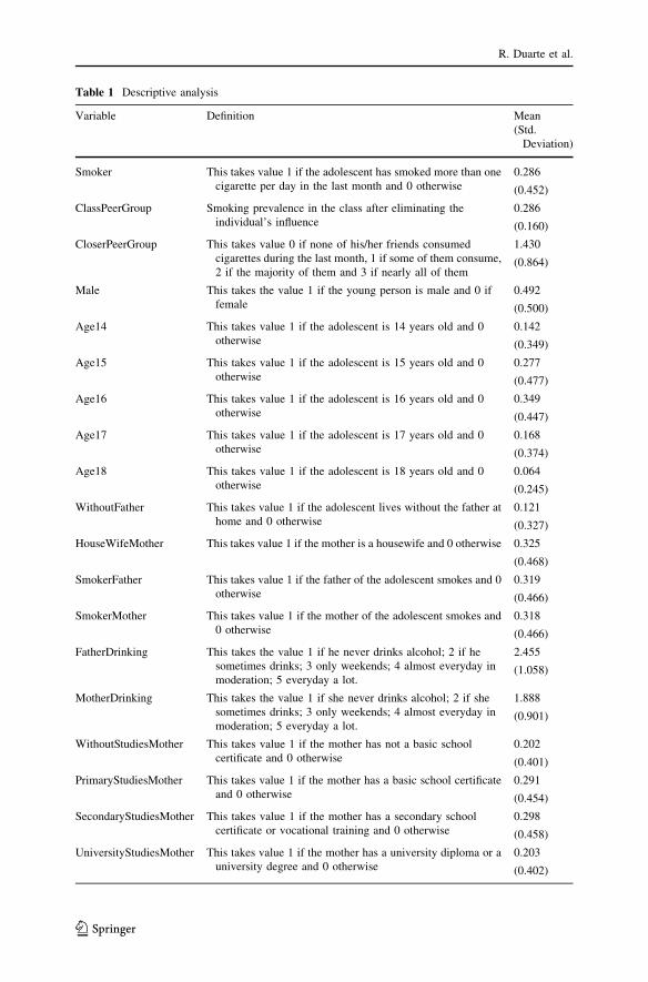
Table 1 Descriptive analysis

Variable Definition Mean

(Std.

Deviation)

Smoker This takes value 1 if the adolescent has smoked more than one

cigarette per day in the last month and 0 otherwise

0.286

(0.452)

ClassPeerGroup Smoking prevalence in the class after eliminating the

individual’s influence

0.286

(0.160)

CloserPeerGroup This takes value 0 if none of his/her friends consumed

cigarettes during the last month, 1 if some of them consume,

2 if the majority of them and 3 if nearly all of them

1.430

(0.864)

Male This takes the value 1 if the young person is male and 0 if

female

0.492

(0.500)

Age14 This takes value 1 if the adolescent is 14 years old and 0

otherwise

0.142

(0.349)


otherwise

0.277

(0.477)


otherwise

0.349

(0.447)


otherwise

0.168

(0.374)


otherwise

0.064

(0.245)

WithoutFather This takes value 1 if the adolescent lives without the father at

home and 0 otherwise

0.121

(0.327)

HouseWifeMother This takes value 1 if the mother is a housewife and 0 otherwise 0.325

(0.468)

SmokerFather This takes value 1 if the father of the adolescent smokes and 0

otherwise

0.319

(0.466)

SmokerMother This takes value 1 if the mother of the adolescent smokes and

0 otherwise

0.318

(0.466)

FatherDrinking This takes the value 1 if he never drinks alcohol; 2 if he

sometimes drinks; 3 only weekends; 4 almost everyday in

moderation; 5 everyday a lot.

2.455

(1.058)

MotherDrinking This takes the value 1 if she never drinks alcohol; 2 if she

sometimes drinks; 3 only weekends; 4 almost everyday in

moderation; 5 everyday a lot.

1.888

(0.901)

WithoutStudiesMother This takes value 1 if the mother has not a basic school

certificate and 0 otherwise

0.202

(0.401)

PrimaryStudiesMother This takes value 1 if the mother has a basic school certificate

and 0 otherwise

0.291

(0.454)

SecondaryStudiesMother This takes value 1 if the mother has a secondary school

certificate or vocational training and 0 otherwise

0.298

(0.458)

UniversityStudiesMother This takes value 1 if the mother has a university diploma or a

university degree and 0 otherwise

0.203

(0.402)

R. Duarte et al.

123

significance and validity discussed in the next section. Second, references in

developmental psychology on non-parental adults support the idea that parents have

little direct influence on the peers of their children, and that children want to

conform to their parents but they do not want to conform to parent’s peers (Galbo

and Demetrulias 1996; Chen et al. 2003). Consequently, adolescents are influenced

by other parents only indirectly through peer behaviour. These are the character-

istics an instrument must fulfil, i.e., it is related to the endogenous regressor but does

not have direct influence on the dependent variable (or it is not correlated with the

error term). Third, it has been pointed out that the importance of the contextual

effects will be reduced by using instruments at the class-level, since when the

reference group is broader, pupils are likely less exposed to the family background

of their peers (Lundborg 2006). Consequently, under the assumption that there are

not contextual effects, the average background characteristics of peers are natural

instruments for average peer smoking (Gaviria and Raphael 2001).

3 Results and discussion

We have implemented two tests in order to have some confidence in the

instruments. The first test is an F-statistic for the joint significance of the

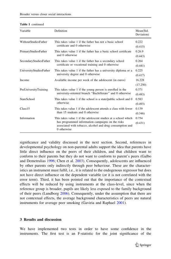
Table 1 continued

Variable Definition Mean(Std.

Deviation)

WithoutStudiesFather This takes value 1 if the father has not a basic school

certificate and 0 otherwise

0.222

(0.415)

PrimaryStudiesFather This takes value 1 if the father has a basic school certificate

and 0 otherwise

0.26.9

(0.443)

SecondaryStudiesFather This takes value 1 if the father has a secondary school

certificate or vocational training and 0 otherwise

0.264

(0.441)

UniversityStudiesFather This takes value 1 if the father has a university diploma or a

university degree and 0 otherwise

0.225

(0.417)

Income Available income per week of the adolescent (in euros) 16.228

(17.250)

PreUniversityTraining This takes value 1 if the young person is enrolled in the

university-oriented branch ‘‘Bachillerato’’ and 0 otherwise

0.371

(0.483)

StateSchool This takes value 1 if the school is a state/public school and 0

otherwise

0.583

(0.493)

Class15 This takes value 1 if the adolescent attends a class with fewer

than 15 students and 0 otherwise

0.139

(0.346)

Information This takes value 1 if the adolescent studies at a school which

has programmed information campaigns on the risks

associated with tobacco, alcohol and drug consumption and

0 otherwise

0.754

(0.431)


123

instruments in the first stage. Second, we follow Wooldridge in order to check the

over-identification restrictions (Wooldridge 2002), i.e., in order to verify that they

are not correlated with the error term. This procedure consists of the following

steps: we first estimate Eq. (1) by two stage least squares including both peer

measures. We then regress the residuals obtained in the previous step on all the

exogenous variables, including the instruments. Finally, the statistic NRu2 of this last

regression follows a Chi squared distribution, under the null hypothesis of the

validity of the instruments, with the degrees of freedom being the number of

indentifying restrictions, this is to say, the number of instruments minus two (the

number of peer variables). The instruments pass both tests whose statistics appear at

the end of table of Table 2.

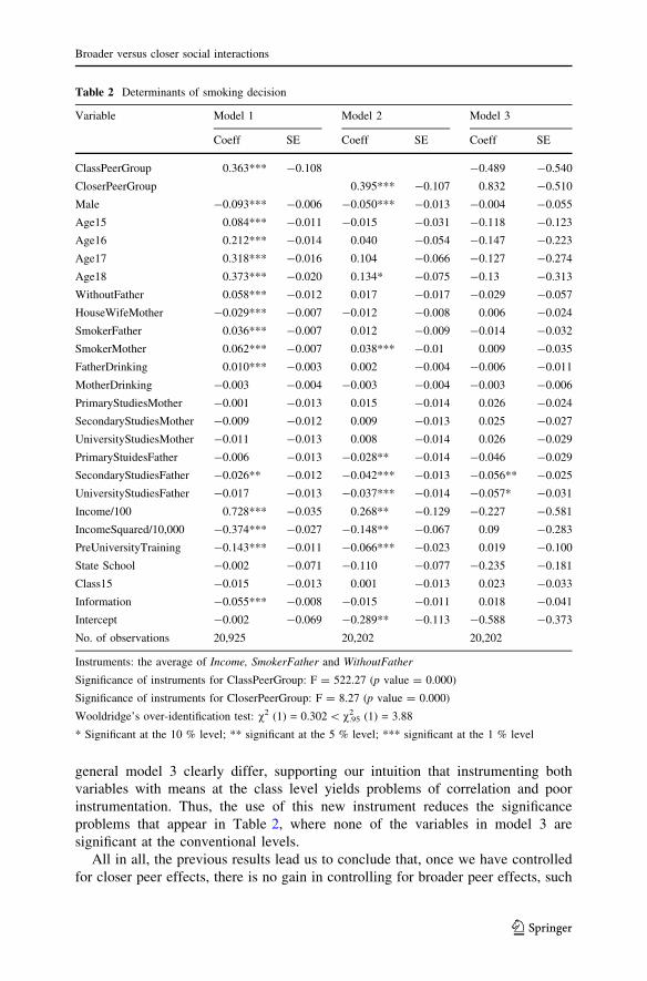
We have estimated three models which appear in Table 2. In the first column, we

use the class-based peer effect variable. In the second column, we replace the class-

based peer variable with our closer peer measure. In the last column, we include

both peer variables. The peer effect estimates are listed at the top of the Table.

A noticeable result is that both peer effects are statistically significant when they

are introduced alternatively. However, the estimates are quite poor when both peer

variables are introduced simultaneously. Thus, all the variables appear to be not

significant at the conventional level. The effect of the closer peer variable appears to

be stronger, statistically speaking, as it would be significant at the 10.2 % level

(p value = 0.102). This low significance can be due to the fact that the instrumented

variables that appear as regressors in the second stage of the 2SLS procedure are

highly correlated (correlation = 0.696), and to the fact that we are instrumenting the

closer peer variable poorly, with instruments that only vary at the class level.

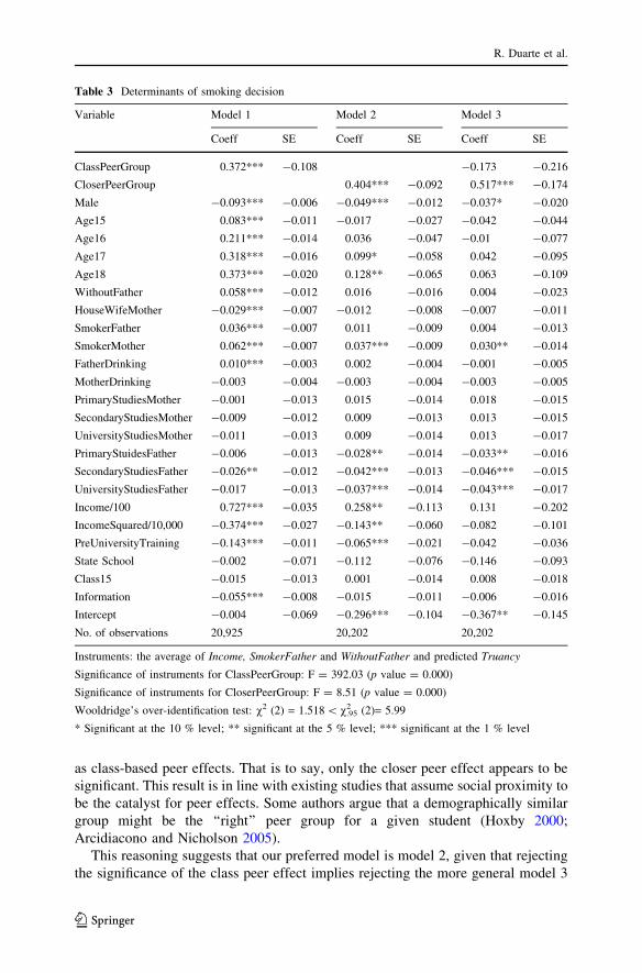
This assumption is supported by the following strategy. We consider re-

estimating the three models to include a new instrument that varies at the individual

level. In order to do so, we include an ‘‘exogenized’’ truancy variable as an

additional instrument. Given that the rude truancy variable may share some

common unobserved individual characteristics with the decision to smoke, we

eliminate these unobserved elements, regressing the truancy variable on the

exogenous variables. Two examples of these unobserved individual characteristics

that can influence both truancy and smoking are rebelliousness and concern about

the future. Thus, for example, there is a greater probability that more rebellious

adolescents and those who are unconcerned about their future will tend to smoke

and skip classes.

Given that the truancy variable is a discrete non-negative variable, we estimate a

model for count data, i.e., a Negative Binomial model. We then use as a new

instrument the predicted part of this variable, which is a function of exogenous

variables and, consequently, we have removed the endogenous unobserved

characteristics. The new set of instruments also passes the tests outlined above

whose statistics appear at the end of table of Table 3.

The estimations of the three models appear in Table 3. An interesting result is

that the coefficients in the first two models barely change in both tables, providing

us with additional evidence that the new instrument is valid. Otherwise, the use of

an endogenous instrument would provide inconsistent estimates and, consequently,

they would differ from those that appear in Table 2. In contrast, the estimates of the

R. Duarte et al.

123

general model 3 clearly differ, supporting our intuition that instrumenting both

variables with means at the class level yields problems of correlation and poor

instrumentation. Thus, the use of this new instrument reduces the significance

problems that appear in Table 2, where none of the variables in model 3 are

significant at the conventional levels.

All in all, the previous results lead us to conclude that, once we have controlled

for closer peer effects, there is no gain in controlling for broader peer effects, such

Table 2 Determinants of smoking decision

Variable Model 1 Model 2 Model 3

Coeff SE Coeff SE Coeff SE

ClassPeerGroup 0.363*** -0.108 -0.489 -0.540

CloserPeerGroup 0.395*** -0.107 0.832 -0.510

Male -0.093*** -0.006 -0.050*** -0.013 -0.004 -0.055

Age15 0.084*** -0.011 -0.015 -0.031 -0.118 -0.123

Age16 0.212*** -0.014 0.040 -0.054 -0.147 -0.223

Age17 0.318*** -0.016 0.104 -0.066 -0.127 -0.274

Age18 0.373*** -0.020 0.134* -0.075 -0.13 -0.313

WithoutFather 0.058*** -0.012 0.017 -0.017 -0.029 -0.057

HouseWifeMother -0.029*** -0.007 -0.012 -0.008 0.006 -0.024

SmokerFather 0.036*** -0.007 0.012 -0.009 -0.014 -0.032

SmokerMother 0.062*** -0.007 0.038*** -0.01 0.009 -0.035

FatherDrinking 0.010*** -0.003 0.002 -0.004 -0.006 -0.011

MotherDrinking -0.003 -0.004 -0.003 -0.004 -0.003 -0.006

PrimaryStudiesMother -0.001 -0.013 0.015 -0.014 0.026 -0.024

SecondaryStudiesMother -0.009 -0.012 0.009 -0.013 0.025 -0.027

UniversityStudiesMother -0.011 -0.013 0.008 -0.014 0.026 -0.029

PrimaryStuidesFather -0.006 -0.013 -0.028** -0.014 -0.046 -0.029

SecondaryStudiesFather -0.026** -0.012 -0.042*** -0.013 -0.056** -0.025

UniversityStudiesFather -0.017 -0.013 -0.037*** -0.014 -0.057* -0.031

Income/100 0.728*** -0.035 0.268** -0.129 -0.227 -0.581

IncomeSquared/10,000 -0.374*** -0.027 -0.148** -0.067 0.09 -0.283

PreUniversityTraining -0.143*** -0.011 -0.066*** -0.023 0.019 -0.100

State School -0.002 -0.071 -0.110 -0.077 -0.235 -0.181

Class15 -0.015 -0.013 0.001 -0.013 0.023 -0.033

Information -0.055*** -0.008 -0.015 -0.011 0.018 -0.041

Intercept -0.002 -0.069 -0.289** -0.113 -0.588 -0.373

No. of observations 20,925 20,202 20,202

Instruments: the average of Income, SmokerFather and WithoutFather

Significance of instruments for ClassPeerGroup: F = 522.27 (p value = 0.000)

Significance of instruments for CloserPeerGroup: F = 8.27 (p value = 0.000)

Wooldridge’s over-identification test: v2 (1) = 0.302 \v.952 (1) = 3.88

* Significant at the 10 % level; ** significant at the 5 % level; *** significant at the 1 % level


123

as class-based peer effects. That is to say, only the closer peer effect appears to be

significant. This result is in line with existing studies that assume social proximity to

be the catalyst for peer effects. Some authors argue that a demographically similar

group might be the ‘‘right’’ peer group for a given student (Hoxby 2000;

Arcidiacono and Nicholson 2005).

This reasoning suggests that our preferred model is model 2, given that rejecting

the significance of the class peer effect implies rejecting the more general model 3

Table 3 Determinants of smoking decision

Variable Model 1 Model 2 Model 3

Coeff SE Coeff SE Coeff SE

ClassPeerGroup 0.372*** -0.108 -0.173 -0.216

CloserPeerGroup 0.404*** -0.092 0.517*** -0.174

Male -0.093*** -0.006 -0.049*** -0.012 -0.037* -0.020

Age15 0.083*** -0.011 -0.017 -0.027 -0.042 -0.044

Age16 0.211*** -0.014 0.036 -0.047 -0.01 -0.077

Age17 0.318*** -0.016 0.099* -0.058 0.042 -0.095

Age18 0.373*** -0.020 0.128** -0.065 0.063 -0.109

WithoutFather 0.058*** -0.012 0.016 -0.016 0.004 -0.023

HouseWifeMother -0.029*** -0.007 -0.012 -0.008 -0.007 -0.011

SmokerFather 0.036*** -0.007 0.011 -0.009 0.004 -0.013

SmokerMother 0.062*** -0.007 0.037*** -0.009 0.030** -0.014

FatherDrinking 0.010*** -0.003 0.002 -0.004 -0.001 -0.005

MotherDrinking -0.003 -0.004 -0.003 -0.004 -0.003 -0.005

PrimaryStudiesMother -0.001 -0.013 0.015 -0.014 0.018 -0.015

SecondaryStudiesMother -0.009 -0.012 0.009 -0.013 0.013 -0.015

UniversityStudiesMother -0.011 -0.013 0.009 -0.014 0.013 -0.017

PrimaryStuidesFather -0.006 -0.013 -0.028** -0.014 -0.033** -0.016

SecondaryStudiesFather -0.026** -0.012 -0.042*** -0.013 -0.046*** -0.015

UniversityStudiesFather -0.017 -0.013 -0.037*** -0.014 -0.043*** -0.017

Income/100 0.727*** -0.035 0.258** -0.113 0.131 -0.202

IncomeSquared/10,000 -0.374*** -0.027 -0.143** -0.060 -0.082 -0.101

PreUniversityTraining -0.143*** -0.011 -0.065*** -0.021 -0.042 -0.036

State School -0.002 -0.071 -0.112 -0.076 -0.146 -0.093

Class15 -0.015 -0.013 0.001 -0.014 0.008 -0.018

Information -0.055*** -0.008 -0.015 -0.011 -0.006 -0.016

Intercept -0.004 -0.069 -0.296*** -0.104 -0.367** -0.145

No. of observations 20,925 20,202 20,202

Instruments: the average of Income, SmokerFather and WithoutFather and predicted Truancy

Significance of instruments for ClassPeerGroup: F = 392.03 (p value = 0.000)

Significance of instruments for CloserPeerGroup: F = 8.51 (p value = 0.000)

Wooldridge’s over-identification test: v2 (2) = 1.518 \v.952 (2)= 5.99

* Significant at the 10 % level; ** significant at the 5 % level; *** significant at the 1 % level

R. Duarte et al.

123

in favour of model 2. Consequently, we will concentrate on model 2 (and refer to

model 1 only in order to compare results with prior research using a similar peer

measure). Moreover, given that using peer measures separately does not yield a

correlation problem, we will focus on the first estimates in Table 2 rather than the

second estimates in Table 3, thus eliminating any existing doubts about the

instrument that varies at the individual level.

It is important to point out that our estimates of models 1 and 2 are in line with

most of the literature. In Ali and Dwyer (2011), for example, the authors estimate

similar models, with the difference being that they use as a closer peer variable the

smoking behaviour of the nominated peers, which our data set does not provide us

with. They also find that both the class and closer peer effect are significant. In

addition, our class peer effect coefficient of 0.363 is very close to the 0.360 reported

in that paper. According to our result, the probability that an adolescent becomes a

smoker will increase by 3.63 points if he/she attends a class with ten percent more

smokers.

In order to interpret the closer peer effect, we should note that the closer peer

variable takes discrete values (0, 1, 2 and 3). Consequently, each unitary increment

of this variable implies that the proportion of friends who smoke is approximately

33 % higher. Thus, when the peer variable increases by one unit, the probability of

being a smoker increases by 39.5 points. This result appears to be very high, as an

increase of this variable from 0 to 3 would imply an increase of 118 points and, for

consistency, the total effect of this variable should not increase the probability by

more than 100 points. However, this does not invalidate our estimates, as we explain

below.

Wooldridge (2002) points out that the Linear Probability Model coefficients are

easy to interpret and often appear to provide good estimates of the partial effects on

the response probability near the centre of the distribution of the explicative

variables. This indicates that the estimated coefficient should give a good

approximation around the mean of the closer peer variable, when passing from 1

to 2, but not necessarily at the extreme values. This suggests that the effects at the

extreme values should be lower, for reasons of consistency.

We can conclude that the probability of being a smoker increases as the

proportion of smoker friends increases. Moreover, and compared with adolescents

with only some friends who smoke, the probability of smoking increases by 39.5

points if the majority of friends become smokers. In addition, it is plausible to

assume that the closer peer effect would be less intense when the number of smoker

friends passes from none to some, and from the majority to all.

If we now focus on the remaining explanatory variables in model 2, we find that

being male reduces the probability of smoking by 5 points. The estimates also

suggest that the probability of smoking is greater, by 3.8 points, among those

adolescents whose mothers smoke. The estimates also indicate that an increase of 10

Euros in disposable income would lead to an increase in the probability of being a

smoker of 2.2 points.

Finally, it is worth highlighting two results that we derive from the analysis of the

marginal effects. First, certain variables that are significant under model 1 are no

longer significant under model 2, that is to say, when we use a narrower measure of


123

the peer variable. Second, although some variables, like Income, appear to be

significant after using a narrower peer group, their quantitative impact is clearly

smaller. This last finding is in line with Lundborg’s suggestion (Lundborg 2006)

that broadly-defined peer groups may not reflect the true reference group and,

consequently, peer group behaviour will be measured with error, and biased

estimates may result.

4 Conclusion

The objective of this paper was to go deeper into the analysis of smokers’ social

interactions by considering simultaneously two peer effects measures. The first is

measured at the class level, and the second is related to the closer group of friends.

We have estimated three linear probability models. In the first, we introduce the

peer effect variable measured at the class level, in the second we include only the

closer peer effect variable, and in the third we introduce both peer effect variables.

Our results reveal that peer effects are important in explaining the decision that

adolescents face about becoming smokers, or not. Although our findings agree with

most of the literature, that peer effects are significant determinants in the smoking

decision, we also provide evidence that the traditional peer variable measured at the

class level is no longer significant when a closer peer measure is introduced. This

constitutes one of the most important findings of our work.

We have found positive and significant peer effects, but we claim that social

interactions occur in the group of friends—not necessarily in the broader school

environment. In this sense, the closer group seems to be more appropriate than the

class group as the ‘‘relevant’’ reference group. The confirmation of these results is

important for policy purposes. Since peer effects can act as ‘‘social multipliers’’, the

identification of the group of friends as a relevant channel would imply that some of

the traditional forms of policy intervention in preventing tobacco consumption

among adolescents, often designed to be conducted in schools, could exert their

influence beyond the school via the relationships with friends that do not attend the

same school.

Manski recognises the difficulty of identifying endogenous peer effects, and the

necessity of knowing the reference group (Manski 1993), but the reference group

is not known a priori. Similarly, Manski (2000) argues that the proper composition

of peer groups is an important unsolved problem in this literature, and little

progress has been made since them. This paper makes a little contribution in this

concern, thus, following the results found, we claim that social interactions occur

in the group of friends and not necessarily in broader school environments. In this

sense, closer group seems to be more appropriate than class group as the

‘‘relevant’’ reference group and we suggest the need for further discussion and

research on the nature and definition of peer groups in order to confirm or reject

our results.

Our study adds to previous literature providing new evidence that smoking is a

widespread behaviour, not just by adult people but also by students aged between 14

and 18 years. It also helps in order to identify the factors that influence on such

R. Duarte et al.

123

behaviour. We have found that physical, family background and school character-

istics are important variables in explaining the decision of being a smoker. The

strong association between mother tobacco behaviour and youth smoking provides

evidence about a possible causal link. This could be due to the fact that mothers that

smoke take less care about this consumption, but also, because children could be

less obedient when mothers do not observe the rules they are trying to impose upon

their children.

As a result, not only should policy makers be involved in the battle of reducing

this dangerous activity, but also families and teachers. Thus, it is clear that smoking

is more likely among females and among older people. As a result, parents should

pay more attention to these groups.

Acknowledgments This work was partially supported by the Spanish Ministry of Science and

Innovation (Project ECO2008-01297). The usual disclaimers apply.

References

Alexander C, Piazza M, Mekos D, Valente T (2001) Peers, schools, and adolescent cigarette smoking.

J Adolesc Health 29:22–30

Ali MM, Dwyer DS (2009) Estimating peer effects in adolescent smoking behavior: a longitudinal

analysis. J Adolesc Health 45:402–408

Ali MM, Dwyer DS (2011) Estimating peer effects in sexual behavior among adolescents. J Adolesc

34:183–190

Arcidiacono P, Nicholson S (2005) Peer effects in medical school. J Public Econ 89:327–350

Chen C, Greenberger E, Farruggia S, Bush K, Dong Q (2003) Beyond parents and peers: the role of

important non-parental adults (VIPs) in adolescent development in China and the United States.

Psychol Sch 40:35–50

Clark AE, Loheac Y (2007) ‘‘It wasn’t me, it was them!’’ Social influence in risky behavior by

adolescents. J Health Econ 26:763–784

De Vries H, Candel M, Engels R, Mercken L (2006) Challenges to the peer influence paradigm: results

for 12–13 year olds from six European countries from the European Smoking Prevention

Framework Approach study. Tob Control 15:83–89

Duarte R, Escario J, Molina J (2006) The psychosocial behaviour of young Spanish smokers. J Cons

Policy 29:176–189

Duarte R, Escario J, Molina J (2013) Are estimated peer effects on smoking robust? Evidence from

adolescent students in Spain. Emp Econ 1–13. doi:10.1007/s00181-013-0704-7

Galbo J, Demetrulias D (1996) Recollections of nonparental significant adults during childhood and

adolescence. Youth Soc 27:403–420

Gaviria A, Raphael S (2001) School-based peer effects and juvenile behavior. Rev Econ Stat 83:257–268

Holliday JC, Rothwell HA, Moore LAR (2010) The relative importance of different measures of peer

smoking on adolescent smoking behavior: cross-sectional and longitudinal analyses of a large

British cohort. J Adolesc Health 47:58–66

Hoxby C (2000) Peer effects in the classroom: learning from gender and race variation. NBER working

paper 7867

Krauth BV (2007) Peer and selection effects on youth smoking in California. J Bus Econ Stat 25:288–298

Lundborg P (2006) Having the wrong friends? Peer effects in adolescent substance use. J Health Econ

25:214–233

Manski C (1993) Identification of endogenous social effects: the reflection problem. Rev Econ Stud

60:531–542

Manski CF (2000) Economic analysis of social interactions. J Econ Perspect 14:115–136

McVicar D (2011) Estimates of peer effects in adolescent smoking across twenty six European countries.

Soc Sci Med 73:1186–1193


123

http://dx.doi.org/10.1007/s00181-013-0704-7

Scheinkman JA (2008) Social interactions (theory). In: Durlauf S, Blume L (eds) New Palgrave

dictionary of economics, 2nd edn. Palgrave Macmillan, Basingstoke

Soetevent AR, Kooreman P (2007) A discrete-choice model with social interactions: with an application

to high school teen behavior. J Appl Econ 22:599–624

Terza JV, Basu A, Rathouz PJ (2008) Two-stage residual inclusion estimation: addressing endogeneity in

health econometric modeling. J Health Econ 27:531–543

WHO (2011) Report on the global tobacco epidemic: warning about the dangers of tobacco

Wooldridge JM (2002) Econometric analysis of cross section and panel data. MIT Press, Cambridge, MA

R. Duarte et al.

123

Documents

Broader versus closer social interactions in smoking