1

Broadband & TCP/IP fundamentals

Sridhar IyerSchool of Information Technology IIT Bombay

sri@it.iitb.ac.inwww.it.iitb.ac.in/~sri

    2

About the course

•  Session 1: Aug 30th (1st half) – Basics of TCP/IP networks: Issues in layering

• Session 2: Aug 30th (2nd half) – Switching and Scheduling: Medium access, switching, 

queueing, scheduling.

• Session 3: Aug 31st  (1st half)–  Routing and Transport: Addressing, routing, TCP 

variants, congestion control

• Session 4: Aug 31st (2nd half) – Applications and Security: Sockets, RPC, firewalls, 

cryptography.

    3

Some Texts/References• A.S. Tanenbaum. Computer Networks. Prentice Hall 

India, 1998.

• S. Keshav. An Engineering Approach to Computer Networks. Addison Wesley, 1997. 

• L.L. Peterson and B.S. Davie. Computer Networks: A Systems Approach. Morgan Kaufmann, 1996. 

• W.R. Stevens. TCP/IP Illustrated, Vol 1: The Protocols. Addison Wesley, 1994. 

• D.E. Comer. and D.L. Stevens. Internetworking with TCP/IP, Vol 1­3. Prentice Hall, 1993. 

    4

More Text/References• W.R. Cheswick and S.M. Bellovin. Firewalls and 

Internet Security. Addison Wesley, 1994. 

• W. Stallings. Cryptography and Network Security. Prentice Hall, 1999. 

• P.K. Sinha. Distributed Operating Systems: Concepts and Design. Prentice Hall, 1997. 

• G. Coulouris, J. Dollimore and T. Kindberg. Distributed Systems: Concepts and Design. Addison Wesley, 1994. 

• RFCs, source code of implementations etc.

    5

Introduction

    6

Layers in a computer

• Hardware: CPU, Memory...• Architecture: x86, Sparc...• Operating system: NT, Solaris...• Language support: C, Java...• Application: dbms...

    7

The network is the computer

• Hardware: Computers and communication media

• Architecture: standard protocols • Operating system: heterogeneous • Language support: C, Java, MPI • Application: peer­peer…

Our focus: network architecture

    8

Perspectives

• Network designers: Concerned with cost­effective design 

– Need to ensure that network resources are efficiently utilized and fairly allocated to different users.

    9

Perspectives (contd.)

• Network users: Concerned with application services

– Need guarantees that each message sent will be delivered without error within a certain amount of time.

    10

Perspectives (contd.)

• Network providers: Concerned with system administration 

– Need mechanisms for security, management, fault­tolerance and accounting.

    11

Connectivity

Building Blocks:• nodes: general­purpose workstations...• links: coax cable, optical fiber...

– Direct links: point­to­point– Multiple access: shared

    12

Switched networks

    13

Interconnection devices

Basic Idea: Transfer data from input to output

• Repeater– Amplifies the signal received on input and 

transmits it on output

• Modem:– Accepts a serial stream of bits as input and 

produces a modulated carrier as output (or vice versa)

    14

Interconnection devices (contd.)

• Hub– Connect nodes/segments of a LAN– When a packet arrives at one port, it is 

copied to all the other ports

• Switch:– Reads destination address of each packet 

and forwards appropriately to specific port– Layer 3 switches (IP switches) also 

perform routing functions

    15

Interconnection devices (contd.)

• Bridge:– “ignores” packets for same LAN 

destinations– forwards ones for interconnected LANs

• Router:– decides routes for  packets, based on 

destination address and network topology– Exchanges information with other routers 

to learn network topology

    16

Network architecture

• Layering used to reduce design complexity– Use abstractions for each layer– Can have alternative abstractions at each 

layer– If the service interface remains 

unchanged, implementation of a layer can be changed without affecting other layers. 

    17

OSI architecture

    18

TCP/IP layers

• Physical Layer: – Transmitting bits over a channel.– Deals with electrical and procedural 

interface to the transmission medium. • Data Link Layer: 

– Transform the raw physical layer into a `link' for the higher layer.

– Deals with framing, error detection, correction and multiple access.

    19

TCP/IP layers (contd.)

• Network Layer: – Addressing and routing of packets.– Deals with subnetting, route determination.

• Transport Layer: – end­to­end connection characteristics.– Deals with retransmissions, sequencing 

and congestion control.

    20

TCP/IP layers (contd.)

• Application Layer: – ``application'' protocols.– Deals with providing services to users and 

application developers.

• Protocols are the building blocks of a network architecture.

    21

Protocols and Services

Each protocol object has two interfaces• service interface: defines operations on 

this protocol. – Each layer provides a service to the layer 

Above.• peer­to­peer interface: defines 

messages exchanged with peer. – Protocol of “conversation” between 

corresponding Layers in Sender and Receiver.

    22

Physical layer – Media dependent components

• Copper: Coaxial/Twisted Pair– Typically upto 100 Mbps 

• Fibre: Single/Multi Mode– Can transmit in Gigabits/second

• Satellite: – Channels of 64 kbps, 128 kbps,…

    23

Physical layer – Media independent

• Connectors: Interface between equipment and link

• Control, clock and ground signals• Protocols: 

– RS 232 (20 kbps, 10 ft)– RS 449 (2 Mbps, 60 ft)

    24

Data link layer functions

• Grouping of bits into frames• Dealing with transmission errors• Regulating the flow of frames

– so that slow receivers are not swamped by fast senders

• Regulating multiple access to the medium

    25

Data link layer services

• Unacknowledged connectionless service – No acknowledgements, no connection– Error recovery up to higher layers – For low error­rate links or voice traffic 

• Acknowledged connectionless service – Acknowledgements improve reliability – For unreliable channels. e.g.: wireless systems

    26

Data link layer services

• Acknowledged connection­oriented service – Equivalent of reliable bit­stream; in­order delivery– Connection establishment and release– Inter­router traffic

• Typically implemented by network adaptor – Adaptor fetches (deposits) frames out of (into) host 

memory

    27

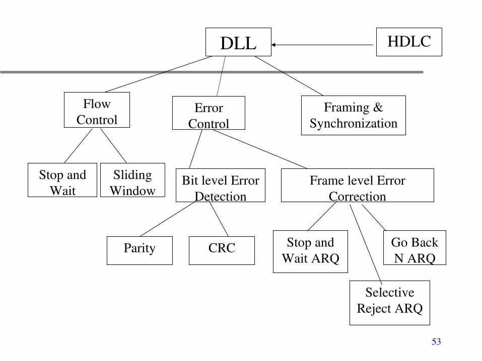
Data link layer – Logical link control (LLC)

• Framing (start and stop)• Error Detection• Error Correction• Optimal Use of Links (Sliding Window 

Protocol)– Examples: HDLC, LAP­B, LAP­D

    28

Data link layer – Medium access control (MAC)

• Multiple Access Protocols• Channel Allocation• Contention, Reservation, Round­robin• Examples: Ethernet (IEEE 802.3), 

Token Ring (802.5)

    29

Network layer

• Need for network layer– All machines are not Ethernet!– Hide type of subnet (Ethernet, Token Ring, 

FDDI)– Hide topology of subnets 

• Scheduling• Addressing• Routing

    30

Network layer functions

• Internetworking– uniform addressing scheme

• Routing– choice of appropriate paths from source to 

destination

• Congestion Control– avoid overload on links/routers

    31

Addressing

Address: byte­string that identifies a node• physical address: device level• network address: network level• logical address: application level

• unicast: node­specific• broadcast: all nodes on the network• multicast: some subset of nodes

    32

Routing

• Mechanisms of forwarding messages towards the destination node based on its address

• Need to learn global information• Queueing (buffering)• Scheduling

    33

Connection Oriented service

• Network layer at sender must set up a connection to its peer at the receiver

• Negotiation about parameters, quality, and costing are possible

• Avoids having to choose routes on a per packet basis

    34

Connectionless service

• Network layer at sender simply puts the packet on the outgoing link without connection setup

• Intermediate nodes use routing tables to deliver the packet to destination

• Avoids connection setup delays

    35

Circuit switching

• dedicated circuit for sender­receiver.• end­to­end path setup before actual 

communication.• no congestion for an established circuit 

connection.• resources are reserved; only 

propagation delays.• unused bandwidth on an allocated 

circuit is wasted.

    36

Virtual Circuits• Used in subnets whose primary service 

is connection­oriented– During connection setup, a route from the 

source to destination is chosen and remembered

– Packets contain a circuit identifier rather than full destination address

• Disadvantages:– Connection setup overhead– If a link/node along the route fails all VCs 

are terminated

    37

    38

Packet switching (datagrams)• Used in subnets whose primary service is 

connectionless• Routes are not worked out in advance

– Successive packets may follow different routes– No connection setup overhead

• Disadvantages : – Packets carry full addresses and are larger– Routing decisions have to be made for every packet– typically ``best­effort" service; may face congestion.

    39

Transport layer

• Lowest end­to­end service

• Main Issues:– Reliable end­to­end delivery– Flow control– Congestion control– providing guarantees

• Depends on application requirements

    40

Application requirements

• Best­effort: FTP• Bandwidth guarantees: Video

– burst versus peak rate

• Delay guarantees: Video– jitter: variance in latency (inter­packet gap)

    41

Bandwidth and Multiplexing

    42

Bandwidth

• Amount of data that can be transmitted per unit time– expressed in cycles per second, or Hertz 

(Hz) for analog devices– expressed in bits per second (bps) for 

digital devices– KB = 2^10 bytes; Mbps = 10^6 bps

• Link v/s End­to­End

    43

Bandwidth v/s bit width

    44

Latency (delay)

• Time it takes to send message from point A to point B– Latency = Propagation + Transmit 

+ Queue–  Propagation = Distance / 

SpeedOfLight– Transmit = Size / Bandwidth

    45

Latency

• Queueing not relevant for direct links• Bandwidth not relevant if Size = 1 bit• Process­to­process latency includes 

software overhead• Software overhead can dominate when 

Distance is small

• RTT: round­trip time

    46

Delay X Bandwidth product

• Relative importance of bandwidth and delay

• Small message: 1ms vs 100ms dominates 1Mbps vs 100Mbps

• Large message: 1Mbps vs 100Mbps dominates 1ms vs 100ms

    47

Delay X Bandwidth product

 100ms RTT and 45Mbps Bandwidth = 560 KB of data

    48

Effective resource sharing

Need to share (multiplex) network resources (nodes and links) among multiple users.

    49

Common multiplexing strategies

• Time­Division Multiplexing (TDM): – Each user periodically gets the entire 

bandwidth for a small burst of time. 

• Frequency­Division Multiplexing (FDM):– Frequency spectrum is divided among the 

logical channels.– Each user has exclusive access to his 

channel.

    50

Statistical multiplexing

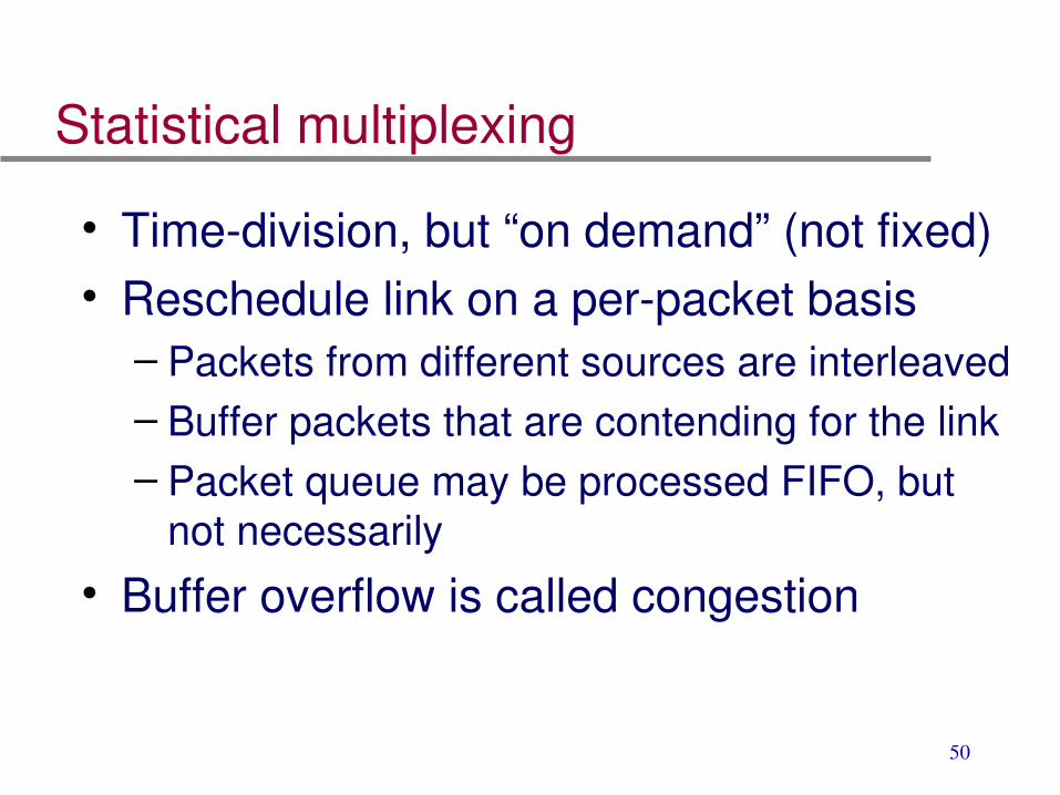
• Time­division, but “on demand” (not fixed)• Reschedule link on a per­packet basis

– Packets from different sources are interleaved – Buffer packets that are contending for the link– Packet queue may be processed FIFO, but 

not necessarily

• Buffer overflow is called congestion

    51

Statistical multiplexing

    52

Error detection and correction

    53

DLL

Stop and Wait

CRCParity

Flow Control

Frame level Error Correction

Bit level Error Detection

Error Control

Selective Reject ARQ

Framing & Synchronization

Go Back N ARQ

Stop and Wait ARQ

Sliding Window

HDLC

    54

Bit level error detection/correction

Single­bit, multi­bit or burst errors introduced due to channel noise. 

• Detected using redundant information sent along with data.

• Full Redundancy: – Send everything twice– Simple but inefficient 

    55

Parity 

Parity (horizontal)• 1 bit error 

detectable, not correctable

• 2 bit error not detectable

Parity (rectangular)• 1 bit error 

correctable• 2 bit error 

detectable• Slow, needs 

memory

    56

Cyclic Redundancy Check (CRC)

• Based on binary division instead of addition. • Powerful and commonly used to ‘detect’ errors.

– Rarely for ‘correction’

• Uses modulo 2 arithmetic:– Add/Subtract  := XOR (no carries for additions or 

borrows for subtraction)– 2^k * M := shift M towards left by k positions and then 

pad with zeros

• Digital logic for CRC is fast. no delay, no storage

    57

CRC algorithm

To transmit message M of size of n bits• Source and destination agree on a 

common bit pattern P of size k+1 ( k > 0)• Source does the following:

– Add (in modulo 2) bit pattern (F) of size k to the message M ( k < n),  such that 

– 2^k * M  + F  = T is evenly divisible (modulo 2) by pattern P.

• Receiver checks if above condition is true– i.e. (2^k * M  + F )/ P = 0

    58

Example

• M = 10011010• P = 1101

M * 2^3 = 10011010000F = 10011010000/1101

= 101T= 10011010000 + 101 

=10011010101 

At receiver• T/P => No remainder

    59

Frame Check Sequence (FCS)

• Given M (message of size n) and P (generator polynomial of size k+1), find appropriate F (frame check sequence)

1. Multiply M with 2^k (add k zeros to end of M)2. Divide (in modulo 2) the product by P

» The remainder R is the required FCS3. Add the remainder R to the product 2^k*M4. Transmit the resultant T

    60

Polynomial representation• Represent n­bit message as an n­1 degree 

polynomial; – M=10011010 corresponds to M(x) = x7 + x4 + x3 + x1. 

• Let k be the degree of some divisor polynomial C(x); (also called Generator Polynomial)– P = 1101 corresponds to C(x) = x3 + x2 + 1. 

• Multiply M(x) by xk;– 10011010000: x10 + x7 + x6 + x4 

• Divide result by C(x) to get remainder R(x); – 10011010000/ 1101 = 101

• Send P(x);10011010000 + 101 = 10011010101 

    61

Generator polynomials

• Receive P(x) + E(x) and divide by C(x)– E(x) represents the error with 1s in position of errors 

• Remainder zero only if: – E(x) = 0 (no transmission error), or – E(x) is exactly divisible by C(x). 

• Choose C(x) to make second case extremely rare.– CRC­8    x8 + x2 + x1 +1– CRC­10  x10 + x9 + x5 + x4 + x1 + 1– CRC­12  x12 + x11 + x3 + x2 + 1– CRC­16  x16 + x15 + x2 + 1– CRC­32  x32 + x26 + x23 + x22 + x16 + x12 + x11 +x10 + x8 + x7 + x5 + x4 + x2 + x + 1

    62

Internet checksum

• IP header; TCP/UDP segment checksum. – View message as sequence of 16­bit integers. – Add these integers using 16­bit ones­

complement arithmetic. – Take the ones­complement of the result. – Resulting 16­bit number is the checksum. – Receiver repeats the operation and matches the 

result with the checksum. 

• Can detect all 1 bit errors.• speed of operation; less erratic channels

    63

Frame level error correction

• Problems in transmitting a sequence of frames over a lossy link– frame damage, loss, reordering, 

duplication, insertion• Solutions:

– Forward Error Correction (FEC)»Use of redundancy for packet level error 

correction– Automatic Repeat Request (ARQ)

»Use of acknowledgements and retransmission

    64

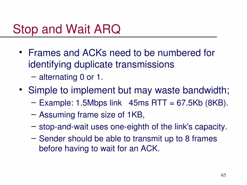
Stop and Wait ARQ

• Sender waits for acknowledgement (ACK) after transmitting each frame; keeps copy of last frame. 

• Receiver sends ACK if received frame is error free and NACK if received frame is in error. 

• Sender retransmits frame if ACK/NACK not received before timer expires. 

    65

Stop and Wait ARQ

• Frames and ACKs need to be numbered for identifying duplicate transmissions – alternating 0 or 1. 

• Simple to implement but may waste bandwidth;– Example: 1.5Mbps link   45ms RTT = 67.5Kb (8KB).– Assuming frame size of 1KB, – stop­and­wait uses one­eighth of the link's capacity.– Sender should be able to transmit up to 8 frames 

before having to wait for an ACK. 

    66

Sliding Window Protocol 

• Allows sender to transmit multiple frames before receiving an ACK.

• Upper limit on number of outstanding (un­ACKed) frames.

• Sender buffers all transmitted frames until they are ACKed. 

• Receiver may send ACK (with SeqNum of next frame expected) or NACK (with SeqNum of damaged frame received). 

    67

Sliding window sender

• Assign sequence number to each frame (SeqNum) • Maintain three state variables: 

– send window size (SWS) – last acknowledgment received (LAR) – last frame sent (LFS) – Maintain invariant: LFS ­ LAR <   SWS 

• When ACK arrives, advance LAR, thereby opening window • Buffer up to SWS frames

    68

Sliding window receiver

• Maintain three state variables: – receive window size (RWS) – last frame accepted (LFA) – next frame expected (NFE) – Maintain invariant: LFA ­ NFE   <  RWS 

• Frame SeqNum arrives: – if SeqNum is in between NFE and LFA, accepted– if SeqNum is not in between NFE and LFA, discarded 

• Send cumulative ACK. 

    69

Sliding window features

• ACKs may be cumulative. – ACK­6 implies all frames upto 5 received 

correctly; – NACK­4 implies frame 4 in error but 

frames upto 3 received correctly. 

• SeqNum field is wrap around.• Window size must be smaller than 

MaxSeqNum.

    70

Go­back­N ARQ

• Sliding window protocol

• Receiver discards out­of­seq pkt received and ACKs LFA. 

• Simplicity in buffering & processing

    71

Selective Repeat ARQ

• Sliding window protocol

• Receiver ACKs correctly received out­of­sequence packets

• Sender retransmits packet upon ACK timeout or NACK (selective reject)

    72

Medium Access Control

    73

Multiple access

problem: control the access so that• the number of messages exchanged per 

second is maximized• time spent waiting for a chance to transmit is 

minimized

medium mediumIntermediatedevices

TransmitterTransmitter/receiver/receiver

TransmitterTransmitter/receiver/receiver

TransmitterTransmitter/receiver/receiver

TransmitterTransmitter/receiver/receiver

    74

Control methods

Where ?• Centralized 

A controller grants access to the network

• DistributedThe stations collectively 

determine the order of transmission

How ?• Synchronous

Specific capacity dedicated to a connection

• AsynchronousIn response to immediate needs 

­> dynamic

•  Free for allTransmit freely

• ScheduledTransmit only during reserved 

intervals

controller server

I1

I2

I3

    75

Performance metrics

• Throughput (normalized) or goodput:–  Fraction of link capacity devoted to 

carrying non­retransmitted packets– excludes time lost to protocol overhead, 

collisions etc. – Example: 1Mbps link can ideally carry 

1000 packets/sec of size 125 bytes; – If a scheme reduces throughput to 250 

packets/sec then goodput of scheme is 0.25. 

    76

Performance metrics (contd.)

• Mean delay– amount of time a station has to wait before it 

successfully transmits a packet• Stability

–  No/minimal decrease in throughput with increase in offered load (number of stations transmitting). 

• Fairness– Every station should have an opportunity to 

transmit within a finite waiting time (no­starvation). 

    77

ALOHA

Stations transmit whenever they have data to send

• Detect collision or wait for acknowledgment• If no acknowledgment (or collision), try again 

after a random waiting time

Collision: If more than one node transmits at the same time.

If there is a collision, all nodes have to re­transmit packets

    78

Vulnerable window 

• For a given frame, the time when no other frame may be transmitted if a collision is to be avoided.

• Assume all packets have same length (L) and require Tp seconds for transmission

• Each packet vulnerable to collisions for time Vp= ??

t

Packet CPacket B

Tp

Packet A

Tp

    79

Vulnerable window

• Suppose packet A sent at time to

• If pkt B sent any time in [to ­ Tp to to]– end of packet B collides with beginning of 

packet A• If pkt C sent any time in [to to to + Tp]

– start of packet C will collide with end of packet A

• Total vulnerable interval for packet A is 2Tp

    80

Slotted ALOHA

• Time is divided into slots– slot = one packet transmission time at 

least• Master station generates 

synchronization pulses for time­slots.• Station waits till beginning of slot to 

transmit.• Vulnerability Window reduced from 2T 

to T; goodput doubles.

    81

ALOHA summary

• Fully distributed, S­Aloha – needs global sync

• Relatively cheap, simple to implement 

• Good for sparse, intermittent  communication. 

• not a good LAN protocol because of – poor utilization (36%)

– potentially infinite delay 

– stations have listening capability, but don’t fully utilize it

• Still used in uplink cellular, GSM

    82

Carrier Sense Multiple Access (CSMA)

• Listen before you speak• Check whether the medium is active before 

sending  a packet (i.e carrier sensing)• If medium idle, then transmit• If collision happens, then detect and resolve

• If medium is found busy, transmission follows:– 1­ persistent– P­ persistent– Non­persistent

    83

1 ­ Persistent CSMA

1 ­ persistent CSMA is selfish• Sense the channel.• IF the channel is idle, THEN transmit.•  IF the channel is busy, THEN continue to 

listen until channel is idle. • Now transmit immediately.

Collisions in case of several waiting senders

    84

P ­ Persistent CSMAp ­ persistent CSMA is a slotted approximation.• Sense the channel.• IF the channel is idle,  THEN 

– with probability p transmit and – with probability (1­p) delay for one time slot and 

start over.

• IF the channel is busy, THEN delay one time­slot and start over.  

    85

Choice of p• Time slot is usually set to the maximum 

propagation delay.• as p decreases, 

– stations wait longer to transmit, but – the number of collisions decreases

• Considerations for the choice of p:–  if np > 1: secondary transmission likely. – So p < 1/n–  Large n needs small p which causes delay

    86

Non­Persistent CSMA

nonpersistent CSMA is less greedy• Sense the channel.• IF the channel is idle, THEN  transmit.• If the channel is busy, THEN wait a 

random amount of time and start over.

• Random time needs to be chosen appropriately

    87

Collision detection (CSMA/CD)• All aforementioned scheme can suffer from 

collision• Device can detect collision

–  Listen while transmitting– Wait for 2 * propagation delay

• On collision detection wait for random time before retrying

• Binary Exponential  Backoff Algorithm– Reduces the chances of two waiting stations 

picking the same random time

    88

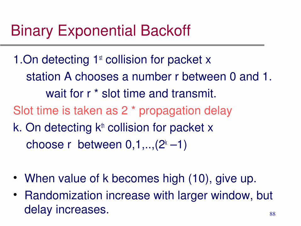
Binary Exponential Backoff

1.On detecting 1st collision for packet x    station A chooses a number r between 0 and 1.          wait for r * slot time and transmit.Slot time is taken as 2 * propagation delayk. On detecting kth collision for packet x    choose r  between 0,1,..,(2k –1)

• When value of k becomes high (10), give up. • Randomization increase with larger window, but 

delay increases.

    89

Example: Ethernet (IEEE 802.3)

• Ethernet Address (48 bits) – Example: 08:00:0D:01:74:71

• Ethernet Frame Format

    90

802.3 frame• Preamble (7 bytes) ­ 0101... • SFD ­ Start Frame Delimiter ­ 10101011 • Length (2 bytes) ­ length (in bytes) of data field • Data (46­1500 bytes) • FCS ­ Frame Check Sequence (4 bytes) ­ error 

checking • May contain LLC header• Minimum size of frame is 64 bytes (51.2µs)

    91

Collision free protocols

• For long cables, propagation delay is increased, decreasing the performance of CSMA/CD.

• Collision free protocols reserve time slots for nodes, thus avoiding collisions.

• Also called as reservation protocols.– Bit map reservation protocol– Adaptive tree walk protocol

    92

Bridging and Switching

    93

Bridges

• connect 2 or more existing LANs– different organizations want to be connected – connect geographically separate LANs.  

• split an existing LAN but stay connected– too many stations or traffic for one LAN– reduce  collisions and increase efficiency– help restrict traffic to one LAN

• Support multiple protocols at MAC layer• Cheaper than routers

    94

Bridge functioning

• Forwards to connected segments• Learns MAC address to segment mapping• Mapping table• Maintains data in table till timeout

    95

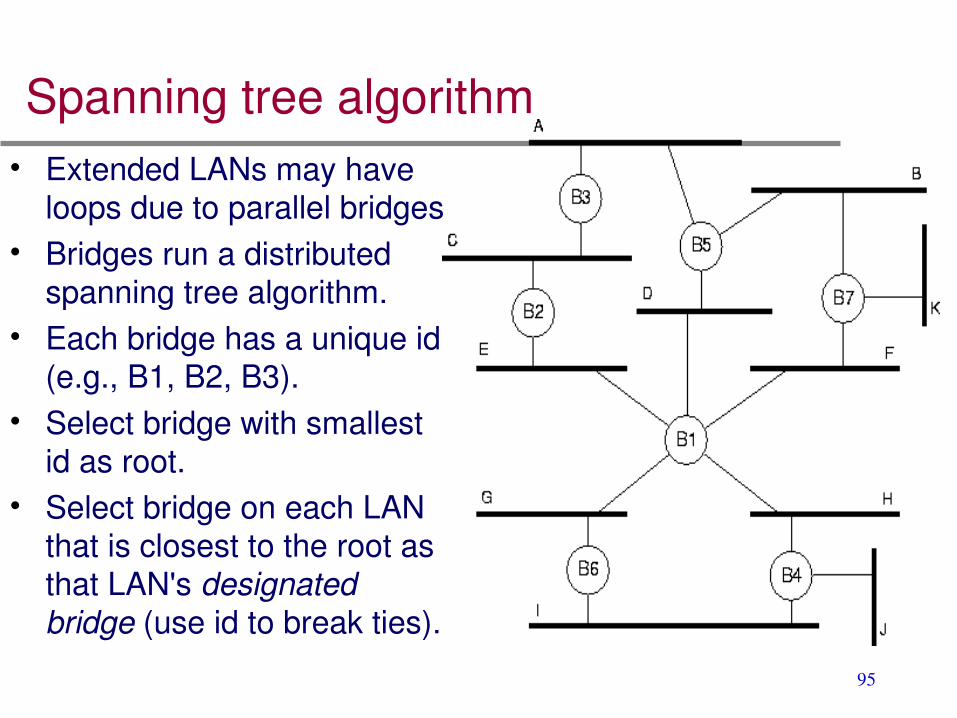
Spanning tree algorithm• Extended LANs may have 

loops due to parallel bridges• Bridges run a distributed 

spanning tree algorithm.• Each bridge has a unique id 

(e.g., B1, B2, B3). • Select bridge with smallest 

id as root. • Select bridge on each LAN 

that is closest to the root as that LAN's designated bridge (use id to break ties). 

    96

Spanning tree protocol• Bridges exchange configuration messages. 

– id for bridge sending the message. – id for what the sending bridge believes to be root bridge. – distance (hops) from sending bridge to root bridge. 

• Each bridge records current best configuration message for each port. 

• Initially, each bridge believes it is the root. • When learn not root, stop generating configuration 

message. • When learn not designated bridge, stop forwarding 

configuration messages. • Root bridge continues to send configuration 

messages periodically.

    97

Generic Switch

Latency: Time a switch takes to figure out where to forward a data unit

    98

Generic Router ArchitectureLookup

IP AddressUpdateHeader

Header Processing

AddressTable

LookupIP Address

UpdateHeader

Header Processing

AddressTable

LookupIP Address

UpdateHeader

Header Processing

AddressTable

QueuePacket

BufferMemory

QueuePacket

BufferMemory

QueuePacket

BufferMemory

Data Hdr

Data Hdr

Data Hdr

1

2

N

1

2

N

N times line rate

N times line rate

    99

Blocking in packet switches

• Can have both internal and output blocking– Internal: no path to output– Output: link unavailable

• Unlike a circuit switch, cannot predict if packets will block

• If packet is blocked, must either buffer or drop it

    100

Dealing with blocking

• Match input rate to service rate– Overprovisioning: internal links much 

faster than inputs

• Buffering: »input port»in the fabric»output port

    101

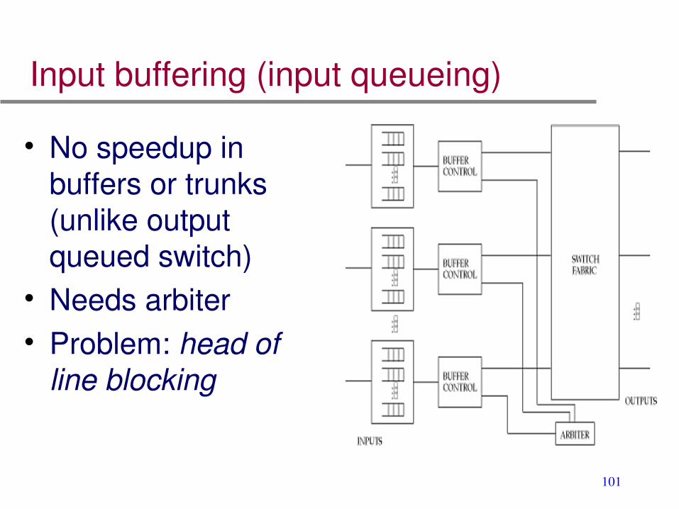
Input buffering (input queueing)

• No speedup in buffers or trunks (unlike output queued switch)

• Needs arbiter• Problem: head of 

line blocking

    102

Output queued switch 

R1Link 1

Link 2

Link 3

Link 4

Link 1, ingress Link 1, egress

Link 2, ingress Link 2, egress

Link 3, ingress Link 3, egress

Link 4, ingress Link 4, egress

Link rate, R

R

R

R

Link rate, R

R

R

R

    103

Scheduling

    104

Packet scheduling

• Decide when and what packet to send on output link– Usually implemented at output interface

1

2

Scheduler

flow 1

flow 2

flow n

Classifier

Buffer management

    105

Scheduling objectives

• Key to fairly sharing resources and providing performance guarantees.

• A scheduling discipline does two things:– decides service order.– manages queues of service requests.

packet voice

e-mail

interactive video

w1

w2

w3

r

Q

    106

Scheduling disciplines• Scheduling is used: 

– Wherever contention may occur– Usually studied at network layer, at output 

queues of switches • Scheduling disciplines: 

– resolve contention – allocate bandwidth – Control delay, loss – determine the fairness of the network – give different qualities of service and 

performance guarantees 

    107

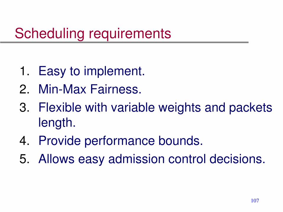
Scheduling requirements

1. Easy to implement.2. Min­Max Fairness.3. Flexible with variable weights and packets 

length.4. Provide performance bounds.5. Allows easy admission control decisions.

    108

Problems with FIFO queues

1. In order to maximize its chances of success, a source has an incentive to maximize the rate at which it transmits. 

2. (Related to #1) When many flows pass through it, a FIFO queue is “unfair” – it favors the most greedy flow.

3. It is hard to control the delay of packets through a network of FIFO queues.

Fair

ness

Dela

y

Gu

ara

nte

es

    109

Fairness

1.1 Mb/s

10 Mb/s

100 Mb/s

A

B

R1C

0.55Mb/s

0.55Mb/s

What is the “fair” allocation: (0.55Mb/s, 0.55Mb/s) or (0.1Mb/s, 1Mb/s)?

e.g. an http flow with a given(IP SA, IP DA, TCP SP, TCP DP)

    110

Fairness

1.1 Mb/s

10 Mb/s

100 Mb/s

A

B

R1 D

What is the “fair” allocation?0.2 Mb/sC

    111

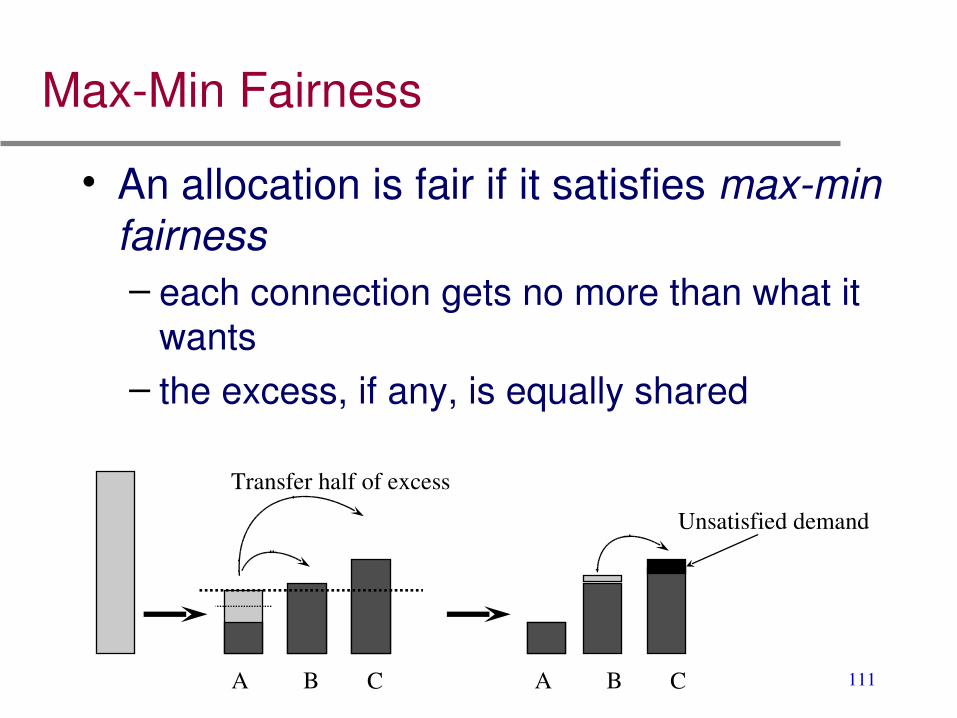
Max­Min Fairness

• An allocation is fair if it satisfies max­min fairness– each connection gets no more than what it 

wants– the excess, if any, is equally shared

A B C A B C

Transfer half of excess

Unsatisfied demand

    112

Max­Min Fairness

• N flows share a link of rate C. • Flow f wishes to send at rate W(f), and is 

allocated rate R(f).1. Pick the flow, f, with the smallest W(f). 2. If W(f) < C/N, then set R(f) = W(f). 3. If W(f) > C/N, then set R(f) = C/N.4. Set N = N – 1. C = C – R(f).5. If N > 0 goto 1.

    113

1W(f1) = 0.1

W(f3) = 10R1

C

W(f4) = 5

W(f2) = 0.5

Max­Min Fairness: example

Round 1: Set R(f1) = 0.1Round 2: Set R(f2) = 0.9/3 = 0.3Round 3: Set R(f4) = 0.6/2 = 0.3Round 4: Set R(f3) = 0.3/1 = 0.3

    114

Fair scheduling goals

• Max­Min fair allocation of resources among contending flows

• Protection (Isolate ill­behaved users)– Router does not send explicit feedback to 

source– Still needs e2e congestion control

• Work Conservation:– One flow can fill entire pipe if no contenders– Work conserving  scheduler never idles 

link if it has a packet

    115

Work conservation

• conservation law: Σρiqi = constant;– ρi  = λixi; – λi is traffic arrival rate – xi is mean service time for packet – qi is mean waiting time at the scheduler, for 

connection i;    • sum of mean queueing delays received 

by a set of multiplexed connections, weighted by their share of the link, is independent of the scheduling discipline

    116

Round robin scheduling

Scan class queues serving one from each class that has a non­empty queue– Assumption: Fixed packet length

• Advantage: – Provides Min­Max fairness and Protection within 

contending flows• Disadvantage:

– More complex than FIFO: per flow queue/state– Unfair if packets are of different length or 

weights are not equal 

    117

Weighted round robin

WA=1.4 WB=0.2 WC=0.8

WA=7 WB=1 WC=4

Normalize

…

round length = 13

• Serve more than one packet per visit• Number of packets are proportional to weights• Normalize the weights so that they become integer

    118

Weighted RR ­ variable length packetIf different connection have different packet 

size, then • WRR divides the weight of each connection 

with that connection’s mean packet size and obtains a normalized set of weights – weights {0.5, 0.75, 1.0}, – mean packet sizes {50, 500, 1500} – normalize weights: {0.5/50, 0.75/500, 1.0/1500} = 

{ 0.01, 0.0015, 0.000666},– normalize again {60, 9, 4} 

    119

Generalized Processor Sharing (GPS)

• Main requirement is fairness– Visit each non­empty queue in turn– Serve infinitesimal from each– GPS is not implementable; we can serve 

only packets

    120

Weighted Fair Queueing (WFQ)

• Deals better with variable size packets and weights

• Also known as packet­by­packet GPS (PGPS)

• Find finish time of a packet, had we been doing GPS; serve packets in order of their finish times

• Uses round number and finish number

    121

WFQ details

• Suppose, in each round, the server served one bit from each active connection

• Round number is the number of rounds already completed– can be fractional

• If a packet of length p arrives to an empty queue when the round number is R, it will complete service when the round number is R + p => finish number is R + p– independent of the number of other connections!

    122

WFQ details

• If a packet arrives to a queue, and the previous packet has/had a finish number of f, then the packet’s finish number is f+p– Serve packets in order of finish numbers

• Finish time of a packet is not the same as the finish number

    123

WFQ Example

A L=1 L=2

B L=2

C L=2

00.5

11.5

22.5

33.5

4

0 1 2 3 4 5 6 7 8real time

virt

ual t

ime

1/3

1/2

1/3

1

F1=1

F1=2

F1=2

F2=3.5

φΑ

A

r = 1

φ A = φ B = φ C = 1

B

C

φΒ

φC

t=0: Packets of sizes 1,2,2 arrive at connections A, B, C.

t=4: Packet of size 2 arrives at connection A

    124

Example (contd.)• At time 0, slope of 1/3,

– Finish number of A = 1, Finish number of B, C = 2 • At time 3, 

– connection A become inactive, slope becomes 1/2• At time 4,  

– second packet at A gets finish number 2 + 1.5 = 3.5, Slope decreases to 1/3

• At time 5.5,– round number becomes 2 and connection B and C 

become inactive, Slope becomes 1• At time 7, 

– round number becomes 3.5 and A becomes inactive.

    125

Guaranteed­service scheduling

• Delay­Earliest Due Date:– packet with earliest deadline selected– Delay­EDD prescribes how to assign deadlines– Source is required to send slower than its peak rate– Bandwidth at scheduler reserved at peak rate– Deadline = expected arrival time + delay bound– Delay bound is independent of bandwidth 

requirement– Implementation requires per­connection state and a 

priority queue

    126

Non work­conserving scheduling

• Non work conserving discipline may be idle even when packets await service– main idea: delay packet till eligible– Reduces delay­jitter => fewer buffers in network– Choosing eligibility time:

» rate­jitter regulator: bounds maximum outgoing rate

» delay­jitter regulator: compensates for variable delay at previous hop

– Always punishes a misbehaving source– Increases mean delay; Wastes bandwidth

    127

Congestion control

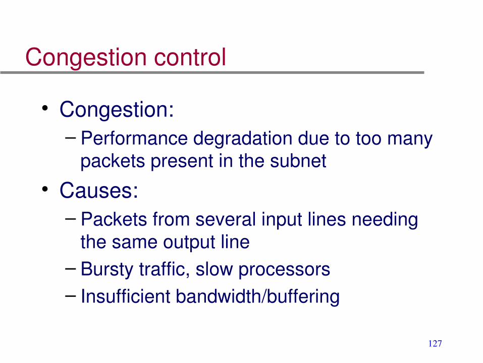
• Congestion: – Performance degradation due to too many 

packets present in the subnet

• Causes:– Packets from several input lines needing 

the same output line– Bursty traffic, slow processors– Insufficient bandwidth/buffering

    128

Congestion control strategies

• Allocate resources in advance• Packet discarding

– aggregation: classify packets into classes and drop packet from class with longest queue

– priorities: drop lower priority packets• Choke the input• Flow control at higher layers 

    129

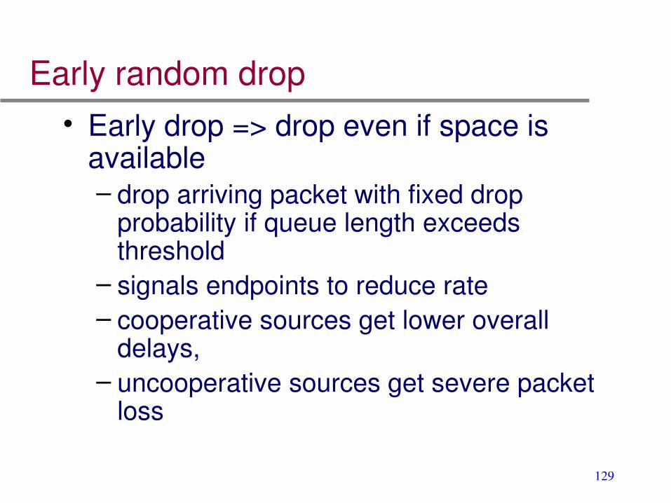
Early random drop• Early drop => drop even if space is 

available– drop arriving packet with fixed drop 

probability if queue length exceeds threshold

– signals endpoints to reduce rate– cooperative sources get lower overall 

delays, – uncooperative sources get severe packet 

loss

    130

Random early detection (RED)

•  Metric is moving average of queue lengths• Packet drop probability is a function of 

mean queue length• Can mark packets instead of dropping 

them• RED improves performance of a network 

of cooperating TCP sources– small bursts pass through unharmed– prevents severe reaction to mild overload

    131

Drop position

• Can drop a packet from head, tail, or random position in the queue

• Tail: easy; default approach• Head: harder; lets source detect loss 

earlier• Random: hardest; if no aggregation, 

hurts uncooperating sources the most

    132

IP Addressing

    133

Addressing

• Addresses need to be globally unique, so they are hierarchical

• Another reason for hierarchy: aggregation– reduces size of routing tables– at the expense of longer routes

    134

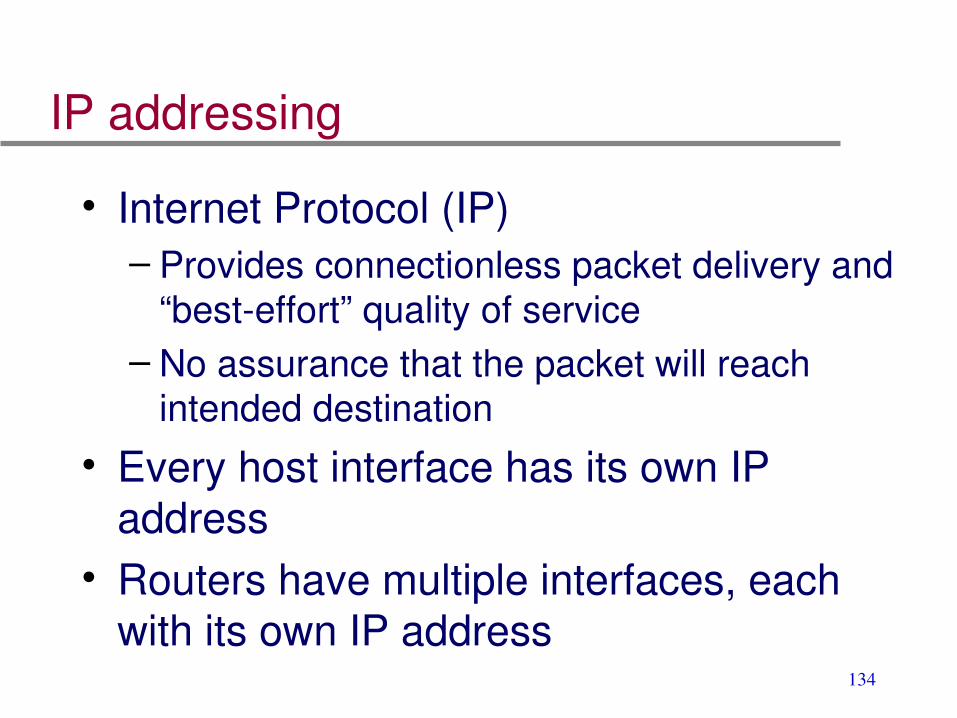
IP addressing

• Internet Protocol (IP)– Provides connectionless packet delivery and 

“best­effort” quality of service– No assurance that the packet will reach 

intended destination

• Every host interface has its own IP address

• Routers have multiple interfaces, each with its own IP address

    135

IPv4 addresses

• Logical address at network layer• 32 bit address space

– Network number, Host number– boundary identified with a subnet mask– can aggregate addresses within subnets

• Machines on the same "network" have same network number 

• One address per interface

    136

Address classes

• Class A addresses ­ 8 bits network number• Class B addresses ­ 16 bits network number• Class C addresses ­ 24 bits network number• Distinguished by leading bits of address

– leading 0 => class A (first byte < 128)– leading 10 => class B (first byte in the range 128­

191)– leading 110 => class C (first byte in the range 

192­223)

    137

IP address notation

• Dotted decimal notation– 144.16.111.2 (Class B)– 202.54.44.120 (Class C)– Special Conventions

»All 0s ­­ this host»All 1s ­­ limited broadcast (localnet)

    138

IP address issues• Inefficient: wasted addresses• Inflexible: fixed interpretation• Not scalable: Not enough network 

numbers• IP addressing schemes 

– Sub­netting: Create sub networks within an address space

– CIDR: Variable interpretations for the network number

– Ipv6: 128 bit address space

    139

Subnetting

• Allows administrator to cluster IP addresses within its network

    140

Classless Inter Domain Routing (CIDR)

• Scheme forced medium sized nets to choose class B addresses, which wasted space– allow ways to represent a set of class C 

addresses as a block, so that class C space can be used

– use a CIDR mask– idea is very similar to  subnet masks, 

except that all routers must agree to use it 

    141

CIDR (contd.)

    142

Address Resolution Protocol (ARP) RFC 1010

• Address resolution provides mapping between IP addresses and datalink layer addresses

• point­to­point links don’t use ARP, have to be configured manually with addresses

RARPARP

32­bit IP address

48­bit Ethernet address

    143

ARP• ARP requests are broadcasts 

– “Who owns IP address x.x.x.x.?”. 

• ARP reply is unicast• ARP cache is created and updated 

dynamically– arp –a displays entries in cache

• Every machine broadcasts its mapping when it boots

    144

RARP and Proxy ARP

• RARP: used by diskless workstations when booting. – Query answered by RARP server

• Proxy ARP: router responds to an ARP request on one of its networks for a host on another of its networks.– Router acts as proxy agent for the 

destination host. Fools sender of ARP request into thinking router is destination

    145

ICMP (Internet Control Message)• Unexpected events are reported to the 

source by routers, using ICMP• ICMP messages are of two types: 

query, error• ICMP messages are transmitted within 

IP datagrams (layered above IP)• ICMP messages, if lost, are not 

retransmitted

    146

Example ICMP messages

• “destination unreachable” (type 3)– can’t find destination network or protocol

• “time exceeded” (type 11)– expired lifetime (TTL reaches 0): symptom of 

loops or congestion . . .• redirect

– advice sending host of a better route• echo request,echo­reply (query)

– testing if destination is reachable and alive• timestamp request, timestamp­reply

– sampling delay characteristics

    147

IP header

    148

IP header• Source and Destination IP addresses of 

4 bytes each• Version number: IPv4, next IPv6• IHL: header length, can be max. 60 

bytes. • 20 byte fixed part and a variable length 

optional part• Total length: max. 65 535 bytes 

presently (header + data)

    149

IP header

• Type of Service (ToS): to be used for providing quality of service – Low delay, high throughput, high reliability, 

low monetary costs are ToS metrics

• TTL: Time to Live, reduced by one at each router. Prevents indefinite looping. 

• Checksum: over header, NOT data.– Implemented in software

    150

IP header

• Protocol: 1=ICMP, 6=TCP, 17=UDP – RFC 1700 for numbers of well known 

protocols– could also be IP itself, for encapsulation

• Identification, 3­bit flags and fragment offset (4 bytes) fields used for fragmentation and reassembly of packets – DF: “Don’t fragment” bit. – MF: More fragments bit.

    151

IP Routing

    152

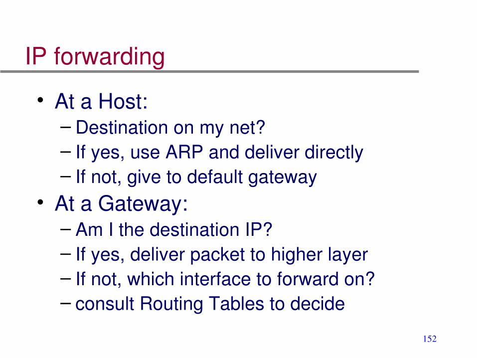
IP forwarding

• At a Host:– Destination on my net?– If yes, use ARP and deliver directly– If not, give to default gateway

• At a Gateway:– Am I the destination IP?– If yes, deliver packet to higher layer– If not, which interface to forward on?– consult Routing Tables to decide

    153

Building routing tables• Computed by routing protocols 

– Routing Information Protocol (RIP) [RFC 1058]

– Open Shortest Path First (OSPF) [RFC 1131]– Border Gateway Protocol (BGP) [RFC 1105]

• Routing table contains the following information– destination IP address (host or network) – IP address of next Hop router– flags: which interface etc.

    154

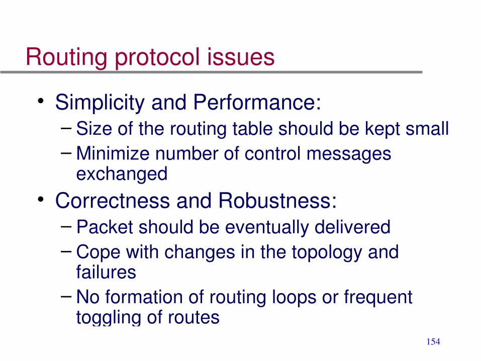
Routing protocol issues

• Simplicity and Performance:– Size of the routing table should be kept small– Minimize number of control messages 

exchanged• Correctness and Robustness:

– Packet should be eventually delivered– Cope with changes in the topology and 

failures – No formation of routing loops or frequent 

toggling of routes

    155

Classification of routing protocols• distance vector vs.  link state

– Both assume router knows»address of each neighbor»cost of reaching each neighbor

– Both allow a router to determine global routing information by talking to its neighbors

• interior vs. exterior– Hierarchically reduce routing information

    156

DV Example: RIP

    157

DV problem: count to infinity

• Path vector– DV carries path to reach each destination

• Split horizon– never tell neighbor cost to X if neighbor is 

next hop to X

• Triggered updates– exchange routes on change, instead of on 

timer– faster count up to infinity

    158

Link state routing

• A router describes its neighbors with a link state packet (LSP)

• Use controlled flooding to distribute this everywhere– store an LSP in an LSP database– if new, forward to every interface other than 

incoming one• Sequence numbers in LSP headers

– Greater sequence number is newer– Wrap around/purging: aging

    159

LS Example: OSPF

    160

RIP• Distance vector

– Cost metric is hop count– Infinity = 16

• RIPv1 defined in RFC 1058– uses UDP at port 520

• trigger for sending of distance vectors– 30­second intervals– routing table update– split horizon

• RIPv2 defined in RFC 1388– uses IP multicasting (224.0.0.9)

    161

OSPF

• Successor to RIP which used Link­State• Using raw IP and IP multicasting • LSP updates are acknowledged• Complex

– LSP databases to be protected

• Implementation: gated

    162

Exterior routing protocols

• Large networks need large routing tables – more computation to find shortest paths– more bandwidth wasted on exchanging DVs 

and LSPs• Hierarchical routing

– divide network into a set of domains– gateways connect domains– computers within domain unaware of outsiders– gateways know only about other gateways

    163

External and summary records

• If a domain has multiple gateways– external records tell hosts in a domain which 

one to pick to reach a host  in an external domain

– summary records tell backbone which gateway to use to reach an internal node

• External and summary records contain distance from gateway to external or internal node

    164

Border Gateway Protocol (BGP)

• Internet exterior protocol• Path­vector

– distance vector annotated with entire path– also with policy attributes– guaranteed loop­free

• Uses TCP to disseminate DVs– reliable– but subject to TCP flow control

    165

Functions of BGP 

• Neighbor acquisition– open and keep­alive messages

• Neighbor reachability– keep alive and update messages

• Network reachability– Database of reachable internal subnets– Sends updates whenever this info changes– notification messages – NLRI: network layer rechability information

    166

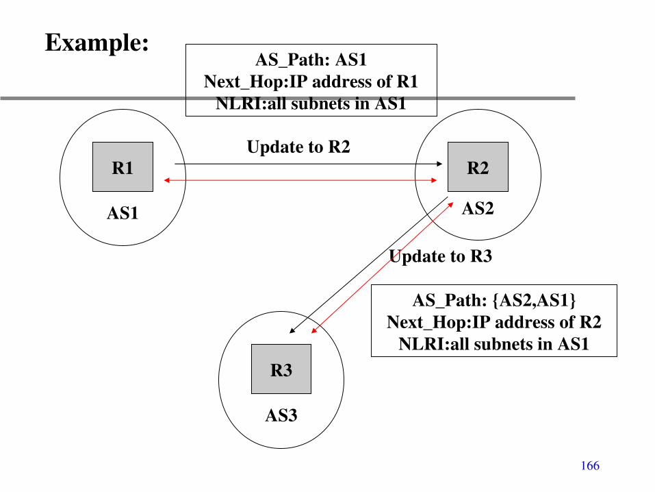
AS_Path: AS1Next_Hop:IP address of R1

NLRI:all subnets in AS1

AS_Path: {AS2,AS1}Next_Hop:IP address of R2

NLRI:all subnets in AS1

R1 R2

R3

Update to R2

Update to R3

Example:

AS1 AS2

AS3

    167

IP routing mechanism

• Steps for searching of routing table– search for a matching host address– search for a matching network address– search for a default entry

• a matching host address is always used before a matching network address (longest match)

• if none of above steps works, then packet is undeliverable

    168

Some IP networking tools

• netstat: info. about network interfaces• ifconfig: configure/query a network interface• ping: test if a particular host is reachable• traceroute: obtain list of routers between 

source and destination• tcpdump/sniffit: capture and inspect packets 

from network• nslookup: address lookup • arp: display/manage ARP cache

    169

End­to­End Transport

    170

User Datagram Protocol (UDP)

• Datagram oriented [RFC 768]• Doesn't guarantee any reliability• Useful for Applications such as voice 

and video, where– retransmission should be avoided– the loss of a few packets does not greatly 

affect performance• each application “write” produces one 

UDP datagram, which causes one IP datagram to be sent

    171

UDP header

• Length of header and data in bytes.• Checksum covers header and data.

– Checksum uses a 12 byte pseudo­header containing some fields from the IP header

– includes IP address of source and destination, protocol and segment length

    172

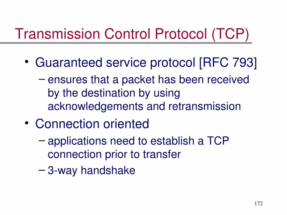
Transmission Control Protocol (TCP)

• Guaranteed service protocol [RFC 793]– ensures that a packet has been received 

by the destination by using acknowledgements and retransmission

• Connection oriented– applications need to establish a TCP 

connection prior to transfer– 3­way handshake

    173

More TCP features

• Full duplex– Both ends can simultaneously read and 

write

• Byte stream– Ignores message boundaries

• Flow and congestion control– Source uses feedback to adjust transmission 

rate

    174

Ports, Connections, End­points, Sockets

TL

144.16.2.1202.15.5.22 149.17.14.3

End PointsConnectionsPort 1143 Port 23

Port 1569 Port 2345

TL TL

    175

Ports and Sockets

• Port: A number on a host assigned to an application to allow multiple destinations

• Endpoint: A pair, a destination host number and a port number on that host

• Connection: A pair of end points• Socket: An abstract address formed by 

the IP address and port number (characterizes an endpoint)

    176

TCP connection and header• Unique identifier for a TCP connection

– Source IP address and port number– Destination IP address and port number

    177

Port numbers

• 16­bit port numbers­ 0 to 65535• 0 to 1023 set aside as well­known ports

– assigned to certain common applications– telnet uses 23, SMTP 25, HTTP 80 etc.

• 1024 to 49151 are registered ports – 6000 through 6063 for X­window server

• 49152 through 65535 are dynamic or private ports, also called ephemeral.

    178

Sequence number and window size• sequence number identifies the byte in 

the stream between sender & receiver.• Sequence number wraps around to 0 

after reaching 232 ­ 1• Window size controls how much data 

(bytes), starting with the one specified by the Ack number, that the receiver can accept

• 16­bit field limits window to 65535 bytes

    179

Flags

• URG: The urgent pointer is valid• ACK: The acknowledgement number is valid 

(i.e. packet has a piggybacked ACK) • PSH: (Push) The receiver should pass this 

data to the application as soon as possible• RST: Reset the connection (during 3­way 

handshake)• SYN: Synchronize sequence number to initiate 

a connection (during handshake) • FIN: sender is finished sending data

    180

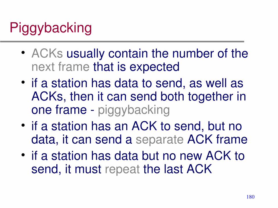
Piggybacking

• ACKs usually contain the number of the next frame that is expected

• if a station has data to send, as well as ACKs, then it can send both together in one frame ­ piggybacking

• if a station has an ACK to send, but no data, it can send a separate ACK frame

• if a station has data but no new ACK to send, it must repeat the last ACK

    181

Connection establishment • Three­way handshake

SYN J, mss 1024

SYN K, mss 1024

ACK J+1

ACK K+1

ServerClient

Segment 2passive open

Connection established

active opensegment 1

Segment 3

    182

Connection termination

ServerClient

FIN M

ACK M+1

FIN N

ACK N+1

Active closesegment 1

Half close

Passive closesegment 2

data

Segment 4

Segment 3

    183

    184

Client Server(active open) SYN_SENT

ESTABLISHED

LISTEN (passive open)

SYN_RCVD

ESTABLISHED

(active close) FIN_WAIT_1

FIN_WAIT_2

TIME_WAIT

CLOSE_WAIT  (passive close)

LAST_ACK

CLOSED

SYN J, mss = 1460

SYN K, ack J+!, mss = 1024

FIN M

ack M+1

FIN N

ack N+1

ack K+1

    185

Timeouts and retransmission

• TCP manages four different timers for each connection– retransmission timer: when awaiting ACK– persist timer: keeps window size information 

flowing– keepalive timer: when other end crashes or 

reboots– 2MSL timer: for the TIME_WAIT state

    186

RTT estimation

• Accurate timeout mechanism is important for congestion control

• Fixed: Choose a timer interval apriori; – useful if system is well understood and 

variation in packet­service time is small. 

• Adaptive: Choose interval based on past measurements of RTT; – Typically RTO = 2 * EstimatedRTT 

    187

Exponential averaging filter• Measure SampleRTT for segment/ACK pair • Compute weighted average of RTT

• EstimatedRTT =  α PrevEstimatedRTT +                                 (1 –  )α  SampleRTT 

• Choose • small α if RTTs vary quickly; large α otherwise• Typically α between 0.8 and 0.9

• Optimizations• Jacobson­Karel; Karn­Partridge algorithms

    188

Flow control

• sliding window flow control: allows multiple frames to be in transit at the same time– Window size may grow or shrink depending 

on receiver and congestion feedback

• Receiver uses an AdvertisedWindow to keep sender from overrunning – Sender buffer size: MaxSendBuffer – Receive buffer size: MaxRcvBuffer 

    189

Advertised window

• Receiving side– AdvertisedWindow = MaxRcvBuffer ­ 

(LastByteRcvd ­ NextByteRead) 

• Sending side– EffectiveWindow = AdvertisedWindow ­ 

(LastByteSent ­ LastByteAcked) 

• Sender uses persist timer to probe receiver when AdvertisedWindow=0. 

    190

Silly­Window syndrome

• slow application receiver – TCP advertises small windows– Sender sends small segments

• solution– Receiver advertises window only if size is 

MSS or half the buffer– Sender typically sends data only if a full 

segment can be sent

    191

Data Transfer using TCP• On a packet count basis, 

– 50% segments bulk data (FTP, E­mail)– 50% segments interactive data (Rlogin)

• On a byte­count basis,– 90% bulk data and 10% interactive – bulk data segments tend to be full sized

• Different algorithms come into play for each

    192

Interactive Input

• Small segments cause congestion• Delayed ACKs are often used to reduce 

number of segments• Nagle algorithm (RFC 896) 

– If TCP connection has outstanding data that has not been ACKed, small segments cannot be sent until ACKs come in

– algorithm is self­clocking: the faster the ACKs come back, the faster data is sent 

– May be turned off e.g. X Window server

    193

Bulk data

• TCP uses the sliding window protocol for efficient transfer of bulk data

• Issues– window size, slow start, congestion…– RTT measurements, congestion avoidance, 

fast retransmit and recovery…

• TCP variants– Tahoe, Reno, Vegas, SACK

    194

Additive increaseMultiplicative decrease • CongestionWindow: limits amount of data 

in transit– MaxWin = MIN (CongestionWindow, 

AdvertisedWindow) EffWin = MaxWin ­ (LastByteSent ­ LastByteAcked) 

• Increase CongestionWindow (linearly) when congestion goes down

• Decrease CongestionWindow (multiply) when congestion goes up

• Source infers congestion upon timeout

    195

Slow start and Congestion avoidance• CongestionWindow: cwnd• AIMD

– Increment cwnd by one packet per RTT– Divide cwnd by two upon each timeout 

• Slow Start– Increase cwnd exponentially upto a threshold 

(ssthresh)• Congestion Avoidance 

– Increase cwnd linearly after ssthresh

    196

Fast retransmit and Fast recovery

• Waiting for TCP sender timeouts leads to idle periods

• Fast retransmit– use duplicate ACKs to trigger retransmission

• Fast recovery– remove the slow start phase; – go directly to half the last successful cwnd 

    197

TCP Tahoe

• Slow start with congestion avoidance• Detects congestion using timeouts• Initialization

– cwnd initialized to 1; – ssthresh initialized to 1/2 MaxWin. 

• Upon timeout – set cwnd to 1, – ssthresh to 1/2 CurrentWindow, – enter slow start. 

    198

TCP Reno

• Detects congestion loss using timeouts as well as duplicate ACKs. 

• On timeout, TCP Reno behaves same as TCP Tahoe. 

• On fast retransmit (receipt of 3 ACKs with same cumulative sequence number),– decreases ssthresh and CurrentWindow to 

half the previous values; skips exponential phase and goes directly into linear increase. 

    199

Application Programming

    200

Application layer• communicating, distributed processes

– exchange messages to implement application– e.g., email, file transfer, the Web

• Application layer protocols– one “piece” of an application– define messages exchanged by application 

components and actions taken– uses services provided by lower layer protocols

    201

Client­Server paradigm

Typical network app has two pieces: 

client and server

applicationtransportnetwork

linkphysical

applicationtransportnetwork

linkphysical

networklink

physicalRequest

Reply

    202

Client­Server actions

• Client:– initiates contact with server (“speaks first”)– typically requests service from server – e.g.: sends request for Web page

• Server– provides requested service to client– e.g., sends requested Web page

    203

Example: Web access (HTTP)

<html>Some network equipment makers:<a href=“http://www.cisco.com”>Cisco</a><a href=“http://www.motorola.com”>Motorola</a></html>

net.html www.it.iitb.ernet.in

Client Req

uest

 for r

esou

rce

http

://w

ww

.it.ii

tb.e

rnet

.in/d

bco.

htm

l

Response:net.html

Some network equipment makers:Cisco   Motorola

HTML renderingof net.html

www.cisco.com

    204

Sockets API• Interface between application and 

transport layer– two processes communicate by– sending data into a socket– reading data out of a socket

• Client “identifies” Server process using– IP address ; port number

    205

Sockets interface

process

TCP withbuffers,

variables

socket

controlled byapplicationdeveloper

controlled byoperating

system

host orserver

process

TCP withbuffers,

variables

socket

controlled byapplicationdeveloper

controlled byoperatingsystem

host orserver

internet

    206

Client actions

• Create a socket (socket)• Map server name to IP address 

(gethostbyname)• Connect to a given port on the server 

address (connect)

• Client must contact server first!

    207

Server actions

• Create a socket (socket)• Bind to one or more port numbers 

(bind)• Listen on the socket (listen)• Accept client connections (accept)• Server process must be running!

    208

Client architecture

• Simpler than servers– Typically do not interact with multiple 

servers concurrently– Typically do not require special ports

• Most client software executes as a conventional program

• Most clients rely on OS for security

    209

Server architecture

Depends on requirements for• Type of connection

– Connection­Oriented: reliable but needs OS resources– Connection­less: less resources but less reliable

• Server state– Stateless: each transaction is independent– Stateful: server maintains state

• Servicing of requests– Iterative:accept requests one at a time– Concurrent:fork a new process for each client

    210

Remote Procedure Call (RPC)

• Goal: make distributed programming as simple as possible– distributed programming should be similar 

to normal sequential programming

• Allow programs to call procedures located on other machines

    211

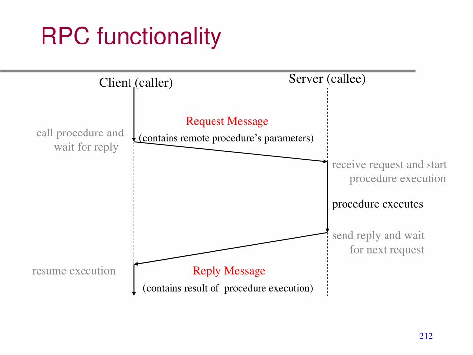
RPC: central idea 

• when program on machine A calls a procedure on machine B, the calling process on A is suspended

• the execution of the called procedure takes place on B

• when the procedure returns, the process on A resumes

• Exchange takes place via procedure arguments and return value

    212

RPC functionality

call procedure and wait for reply

resume execution

Server (callee) 

receive request and start procedure execution

send reply and wait for next request

procedure executes

Request Message (contains remote procedure’s parameters)

Reply Message (contains result of  procedure execution)

Client (caller) 

    213

RPC design

Client Server

Client Stub Server Stub

Client Procedure Called Procedure

Network transport Network Transport

arguments results

Network

    214

RPC advantages

• Extends the conventional procedure call to the client/server model

• Remote procedures accept arguments and return results

• Makes it easy to design and understand programs

• Helps programmer to focus on the application instead of the communication protocol

    215

Network Security

    216

Network security

• Security Plan (RFC 2196)– Identify assets– Determine threats– Perform risk analysis– Implement security mechanisms – Monitor events, handle incidents

• Cost of protecting should be less than the cost of recovering

    217

Security requirements

• Confidentiality:– No unauthorized disclosure 

• Integrity:– No unauthorized modification

• Authentication:– Assurance of identity of originator 

• Non­Repudiation:– Originator cannot deny sending the 

message

    218

Security threats and levels

• Threats– Host: Unauthorized access– Transmission: sniffing, masquerading

• Host level – Authentication and access control

• Network level – Firewalls and proxies

• Application level – Encryption and signatures

    219

Firewalls

    220

Sample filtering rules

• Permit incoming Telnet sessions only to a specific internal hosts

• Permit all outbound Telnet and FTP sessions

• Deny all incoming traffic from specific external networks

    221

Cryptography

Components:

• Plain text• Encryption/Decryption Algorithms• Encryption/Decryption Keys• Cipher text

    222

Techniques

• Symmetric/Private Key: (DES)– secure environment for key exchange

• Asymmetric/Public Key: (RSA)– private­public key pair

• Hash Algorithms: (MD5, SHA)– message integrity 

• Digital Signatures: – integrity and authentication

    223

    224

Some security tools

• Password tools: crack, COPS • Host­based auditing tools: Tripwire, rdist • Virus detection software: Norton, McAfee • Network­based auditing tools: SATAN, SAINT • Network traffic analyzers: tcpdump, sniffer • Firewall packages/products: Checkpoint, PIX • Encryption utilities and libraries: PGP 

    225

Summary

• Multiplexing• Error detection and correction• Medium access control• Switching and scheduling• Addressing and routing• Flow and congestion control• Application API• Security